MULTISUPPLIER PROCUREMENT UNDER UNCERTAINTY IN
INDUSTRIAL FISHING ENVIRONMENTS
A THESIS SUBMITTED TO THE GRADUATE SCHOOL OF
SAINT MARY'S UNIVERSITY
BY
Melvina Marius
IN PARTIAL FULFILLMENT OF THE REQUIREMENTS
FOR THE DEGREE OF
MASTER OF SCIENCE
Melvina Marius, June 2003
1 ^ 1National Ubwy of Canada
Acquisitions and BARogmphkSenfices386W ##nglonSb##( OamwmON K1A0N4
Bküothèque du Canada
Acquisitions et services bbüographiquesaoS.meWeangkn
lON K1A0N4
% Vbw rê^èfWiOÊ
The audior bas granted a non- exchmve licence allowing the National Libraiy of Canada to iqKodnce, loan, distribute or sell copies of this dxesis in microharm, pagw or electronic formats.
The author retains ownersh^ of the copyright in this thesis. Neither the Aesis nor substantial extracts from it may be printed or otherwise reproduced wiAout die author's permission.
L'auteur a accordé une hcence non exclusive permettant à la Bibhothéque nationale du Canada de reproduire, prêter, distribuer ou vendre des copies de cette thèse sous la forme de microhche/Ghn, de reproduction sur p^ier ou sur farmat électronique.
L'auteur consove la propriété du droit d'auteur qui protège cette thèse. Ni la thèse ni des extraits substantiels de celle-ci ne doivent être imprimés ou autrement reproduits sans son autmisatiorL
0-612-85292-X
Canada
Name:
Degree:
Title of Thesis:
Cerdëcaüon
Melvina Marius
Master of Science in Applied Science
Multi-Supplier Procurement Under Demand and Supply Yield Uncertainty
Examining Committee:
William E. lo n e^ Acting of Graduatdatudies
of Science
Dr. Harvey Millar, Senior Supervisor
Dr. PemberO ,, Supervisory Committee
Dr. Muhong Wang, Supervisory Committee
Dr. Paul lyogun. External Examiner Department of Business, Wilfred Laurier University Waterloo, Ontario
Date Certified: June 18,2003
TABLE OF CONTENTS
TABLE OF CONTENTS...........................................................................................H
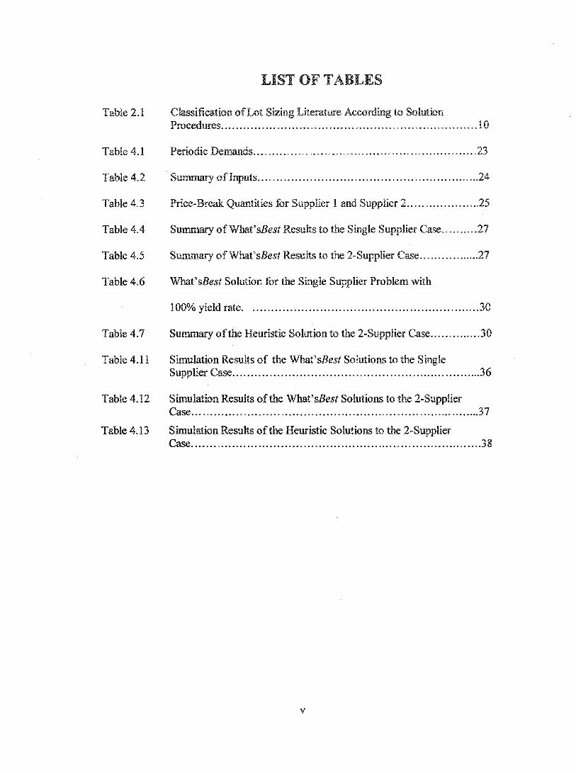
LIST OF TABLES.....................................................................................................iv
LIST OF FIGURES....................................................................................................v
ACKNOWLEDGEMENTS......................................................................................vi
ABSTRACT...............................................................................................................vü
CHAPTER 1 INTRODUCTION
1.1 Introduction..................................................................................................1
1.2 Objectives and Scope o f this research.........................................................3
1.3 Organization of the Thesis.......................................................................... 4
CHAPTER 2 SURVEY OF INVENTORY LOT SIZING PROBLEMS
2.1 Introduction....................................................................................................5
2.2 Yield Uncertainty in Inventory Lot-Sizing................................................. 6
2.3 Survey o f Multi-Supplier Lot- Sizing Problems........................................ 7
2.4 Survey o f Lot-Sizing Problems with Supplier Selection and
Quantity Discounts......................................................................................9
2.5 Solution ^p ro ach es.................................................................................. 10
2 . d. y A/eurü/ic ProceeA/rcf.......................................... 11
2. d. 2 Mz/Aemu/fco/ Progrwnmfng Buscf/ f / e w / f ...........12
u
CHAPTER 3 MOTIVATION, FORMULATION AND SOLUTIONMETHODOLOGY
3.1 Introduction............................................................................................. 15
3.2 Definition o f the Problem and Notation................................................16
3.2.7 VbtafioM...................................................................................... 17
3.3 Mathematical Programming Formulation............................................. 18
3 .4 Solution Methodology............................................................................19
3.4.7 tTze AewMtfc............................................................21
CHAPTER 4 COMPUTATIONAL STUDY
4.1 Introduction............................................................................................ 23
4.2 NunKrical Analysis............................................................................... 23
4.3 Computational Results.......................................................................... 27
4.3.7 Sb/znfoM IFMf fR cft................................................ 27
^.3.2 7!eWtf T&wig/fc 30
4.4 Sensitivity Analysis..............................................................................33
4.^.7 Æ ç% nmenfa77)ef^................................................................34
< 7 7(eWfs................................................................... 36
CHAPTER 5 SUMMARY AND CONCLUSION
5.1 General Results Obtained From the Model..........................................41
5.2 Conclusion...............................................................................................42
5.3 Future Research...................................................................................... 43
111
LIST OF TABLES
Table 2.1 ClassiScation o f Lot Sizing Literature According to SolutionProcedures.......................................................................................... .10
Table 4.1 Perwdic Demands................................................................................... 23
Table 4.2 Summary o f Iiqiuts................................................................................... 24
Table 4.3 Price-Break Quantities for Supplier 1 and Supplier 2 ............................25
Table 4.4 Summary o f What'sBesf Results to the Single Supplier Case..............27
Table 4.5 Summary o f WhaCsBest Results to the 2-Supplier Case...................... 27
Table 4.6 What'sBest Solution &r the Single Supplier Problem with
100% yield rate........................................................................................ 30
T*d)le 4.7 Summary o f the Heuristic Solution to the 2-Supplier Case................... 30
Table 4.11 Simulation Results o f the What'sBesf Solutions to the SingleSupplier Case............................................................................................36
Table 4.12 Simulation Results o f the Whal'sBesf Solutions to the 2-SupplierCase.......................................................................................................... 37
Table 4.13 Simulation Results o f the Heuristic Solutions to the 2-SupplierCase............................................................................................................38
LIST OF FIGURES
Figure 4.1 Total Costs 6 )r Each Supplier Scenario Under VaryingLevels o f Yield Rates............................................................................. 31
Figure 4.2 Inventory Related Cost Each Supplier ScenarioUnder Varying High Yield R ates......................................................... 39
Figure 4.3 Inventory Related Cost k r Each SupplierScenario Under Varying Low Yield R ates.............................................39
VI
ACKOWLEDGEMENTS
I wish to thank my supervisor. Dr. Harvey Millar, 6 )r all his valuable advice throughout
my studies. In addition to his exceptional guidance on this work he demonstrated to me
how to efkctively conduct research in general 1 am gratehil to Dr. Millar and Saint
Mary's University for funding my research through the Research Assistantship Grants.
I wish to thank my examining committee. Dr. Harvey H. Millar, Dr. J Cryus, Pemberton
Dr. Muhong Wang, and the external examiner Dr. Paul lyogun 6 )r their time and ef&rt in
evaluating this thesis.
I would also like to thank my &mily, especially my two children Janique and Kussel, for
all their understanding, siq)port and help during my studies.
vn
Multisupplier Procurement Under Uncertainty in Industrial FishingEnvironments
Melvina MariusSubmitted June 18,2003
ABSTRACT
In this paper we address the issue of multi supplier sourcing as a tool for hedging against supply yield uncertainty. Our work was motivated by the problems in the fishing industry whereby fish processing firms are constantly faced with the problems of random supply yields. We formulated a mathematical programming model that can be used to determine the quantities to be ordered 6 0 m two or more suppliers so as to minimize annual expected procurement cost while attempting to satisfy demand requirements and operating constraints. The cost included are purchasing cost, inventory related cost and ordering cost. We assume that at the beginning of a planning horizon comprised of 12 periods a him enters into minimum contractual agreement with two suppliers, and in return each supplier offers a discounted price schedule.
In our numerical analysis we solved the model for both the 2-supplier case and the single supplier case and compared the cost of using a single supplier versus two suppliers under varying levels of yield variability. We compared deterministic solutions for the single and two-supplier case and use Monte Carlo simulation to assess the robustness of the solutions under varying levels of yield uncertainty. Results show that as the variability of the yield rate increases it becomes cost effective to use two suppliers as a means for hedging against uncertainty. We compared the results &om our model to that of a heuristic procedure proposed by Parlar and Wang, an alternative approach for solving the 2-supplier inventory problem. The results indicated that our model provides superior solutions to that of the heuristic procedure.
vui
CHAPTER 1
Introduction
1.1 Introduction
Purchasing decisions are becoming increasingly strategic 5)r many organizations. Many
are now looking to their suppliers to help them attain a strong competitive market
position. Selecting the most appropriate suppliers is an inqwrtant strategic management
decision that may inexact all areas o f an organization (Jayaraman et al 1999). A large
percentage of the total cost Bar many organizations is from purchases, thus the reduction
o f purchasing cost is the m ^ r concern of managers.
A m ^ r decision 6 ced by purchasing managers is determining the conEguration o f the
supp^ base. For example, working with a few atppliers enables a firm to enter into
long-term contractual relationships. On the other hand purchasing managers may want to
split their orders when 6 ced with the need to reduce risk in the conditions characterized
by uncertainty in demand and supply yields and as a means o f maintaining corrgietition
amor% a set o f suppliers.
Faced with a dramatic decline in the ground Gsh resource in Atlantic Canada, Gsh
processing industry firms are &rced to obtain fish resources hom external suppliers.
Because o f the nature o f the fishing industry, Gsh harvesters mq)erience less than per&ct
yields. For this reason, a siqiplier's ability to meet a firm's demand for raw 6 sh is
uncertaiiL This can create periodic shortages, which may prove detrimental to the buyers.
As such techniques &)r handling supply uncertainty is critical to the conqietitiveness o f
fish processing firms. There&re, firms must determine an eSective strategy that would
enable them to determine the best ordering policies, to maximize total yield and minimize
average annual cost associated with procurement.
The siqyplier selection and allocation decisions made may incorporate minimum
commitment contracts. Many researchers have shown the benefits of commitment
contracts (Anupindi and Bassok (1999), Serel et aL (2001), Larviere (1998)). By
committing to purchasing a minimum quantity, the buyer can negotiate a better price, and
the supplier will be provided with the guarantee that his/her 6 sh will be sold. In return for
the buyer's commitment, the siq)plier provides a price discount.
Purchasing 6 sh 6 om more than one supplier is necessary to sustain a desirable service
level and to reduce the total system cost incurred when acquisition lead-time and order
quantities are uncertain. In a mufti-siqiplier system, deliveries hom all suppliers do not
take place at the same time and are distributed over different intervals over a period of
time. Thus when supply yield is uncertain the chance o f shortages can be reduced. That is
to say that multi-supplier sourch% can 6 cilitate splitting an order to consider the
variability in arrival time and the quantity of Gsh delivered.
1.2 Objectives and Scope of this Research
There are 6 w models that address the issue of yield uncertainty in industrial Gshing
environments. For this reason our paper is based on the 5)Uowing objectives;
1. To gain insight into the deterministic representation of the random yield problem
2 To congiare the cost o f using two suppliers to the cost associated with a single
supplier under supply uncertainty
3 To use discrete simulation to compare the cost of two supplier sourcing versus
single supplier sourcing under varying levels of supply yield rates
3. To ascertain the efkctiveness o f multi-supplier sourcing as a strategy 6 )r hedging
g ain st the ef&ct o f supply yield uncertainty
This research presents a formulation and solution methodology for the multi-supplier lot-
sizing px)blem under conditions o f uncertainty. The problem is not modeled as a
stochastic problem but rather as a deterministic problem based on the mean values 6 r
random yield rates. The model is formulated as a non-linear mathematical program with
quantity discounts and minimum commitment. It will be solved using a commercial non
linear solver called "What'sBesf" developed by LINDO Systems INC.
1.3 Organization of the Thesis
The next chapter presents the background to the problem and cites the relevant literature.
Chapter three describes the mathematical formulation o f the model and the solution
procedure. The computational study and reports on the computational results are
presented in chapter 6 )ur. Finally, chapter five concludes with a brief summary and
discussion o f future research possibilities.
CHAPTER 2
Literature Review of inventory Lot-sizing Probiems
2.1 Introduction
The lot-sizing procurement problem is to determine when to order and how much to order
given the demand o f a product so as to minimize total procurement cost with demand
being either stochastic or deterministic.
The earliest solution to the lot-sizing problem was the Economic Order Quantity Model
(EOQ) developed by Harris (1913). The EOQ nxxiel is a continuous time model that
seeks to minimize total inventory cost by making optimal order quantities under certain
conditions. It assumes that the demand 5)r a single product is constant and deterministic
with a known fixed set up cost. Backlogging and shortages are not allowed. There is no
capacity constraint and delivay is instantaneous. This means that there is no delay
between placing an order and receiving that order. With the EOQ it is always optimal to
place an order when the inventory level is at zero. The EOQ can be easily applied to other
inventory situations and provides good starting solutions far more conq)lex models. For
this reason it has been used as the basis 6 r a number o f heuristic solutions. Examples o f
this approach can be 6 )und in Mazzola et al. (1987), Silver (1976), and Parlar and Berkin
(1991).
Mæntainmg most o f the assunqAions of the classical EOQ Wagner and Whitin (1985)
developed an algorithm for solving the dynamic lot-sizing problem. They based their
model on the proper^ that under an optimal lot-sizing policy there exists an optimal plan
such that the inventory carried out 6 om a previous period / to period f + 1 will be zero or
the production quantity in period r +1 will be zero. Like the EOQ the Wagner and Whitin
algorithm is being used by many researchers as the basis &)r solving dynamic lot sizing
inventory problems. See Britran et aL (1984), Wagleman (1992) and Aggarwal and Park
(1993).
2.2 Yield Uncertainty in Inventory Lot-Sizing
Both the EOQ and the Wagner-Whitin algorithm are based on the assunq)tion that
product delivery is irmnediate and the amount ordered is the amount received. However
in real li& situations many Srms are 6 ced with yield randomness. For this reason
researchers have seen the need to incorporate yield randomness into inventory problems.
Yield uncertainty is viewed in two difkrent ways in inventory k)t-sizir%. It can be
viewed as uncertain lead-time where delivery is not immediate and as uncertain delivery
where the quantity delivered is a Auction of the quantity requested.
The problem has been addressed in various krm s by many authors such as Ehrhardt and
Taube (1987), Gerchark et aL (1986), Gerchak and Wang (1994, Amihud and Medelson
(1993), Kelle and Silver (1990), I Ian and Yardin (1885), Nahmias and Moinzaden (1997)
and Parlar (1997). An extensive survey of literature on the concept can be &)und in Yano
and Lee (1995), who presented a survey on quantitative oriented approaches to solving
the random yield lot-sizing problem.
2.3 Survey Of Multi- Supplier Lot-Sizing Problems
Research on multi-supplier inventory systems began in 1981, by Sculli and Wu. They
considered an inventory item with two suppliers where the lead times are normally
distributed and the reorder level is the same 6 r both suppliers. Since then many other
researchers have considered such systems.
Hayya et a l (1987) reiterated Sculli and Wus' model using simulation and Sculli and
Shum (1990) extend their results to the case o f n>2 suppliers. Gerchak and Parlar (1990)
considered the diversiScation strategy when two independent suppliers have difkrent
yield rates. They examined the problem of determining the optimal lot sizes to be ordered
simultaneously 6 om the suppliers to meet demand and minimize cost. Yano (1991)
exteixl this model to investigate the issue when quality is reflected in the yield rate
distribution, and where two suppliers are used 6 )r strategic reasons. Yano (1991) modeled
the case where the customer alternately orders hom the two suppliers.
Parlar and Wang (1993) extended the results 6 und in Gerchak and Parlar (1990) by
making the assumption that the prices charged by the two suppliers and the unit holding
cost incurred for the items purchased horn the two suppliers are difkrent. They
developed a convex total cost expression function of the order quantities 6 om each
supplier.
Anupindi and Akella (1993) addressed the operational issue o f quantity allocation
between two uncertain suppliers and its efkcts on the inventory policies of the buyer.
They assumed that demand is stochastic and continuously distributed with a known
distribution and developed three naodels 6 )r supply processes.
Lau and Zhoa (1993) developed a procedure that determines the order policy that
optimizes the inventory system cost when the daily demarxi and suppliers' lead-time are
all stochastic. Lau and Zhoa (1994) presented an easily solvable version of the procedure
where there existed no restrictions on lead- time distribution and order q)lit proportion.
These papers generally studied two-supplier systems. Nevertheless, other researchers
have considered multiple-supplier systems. Among these are Tempelmeier (2001), Millar
(2000 a) and Millar (2000 b), who developed a model 6 r assessing m uki-su^lier versus
single supplier sourcing under deterministic conditions and varying supply. Sedarage et
aL (1999) considered a general n-supplier single item inventory system where the item
acquisition lead times o f suppliers and demand arrival is random. They developed an
optimization model to determine the reorder level and order split quantities for n-
suppliers.
2.4 Survey of Lot-SWng Problems with Supplier Selection and
Quantity Discounts
Solutions to lot-sizing problems under considerations o f quantity discounts have been on
going 6 )r some time. Benton and Park (1996) presented a paper, vdiich classified and
discussed some o f the significant literature on lot-sizing under several types of discount
schemes. They observed that most o f the studies thus 6 r have investigated single buyer
and single siq)plier situations with a single or a small number o f price breaks. Examples
o f papers in this area are by Chaundry et al (1993), Kasilingam and Lee (1996), Jayayam
et al (1999) and Geneshan (1999) who all studied the sii^le period problem. The multi
period problem was considered by Gaballa (1974), Buf& and Jackson (1983), Pikul and
Aras (1995), Sharma et aL (1989) and Benton (1991).
V ^h the enq)hasis on siqiply chain management many firms see the need to enter into
contractual agreements with their suppliers. Consequently there has been an increasing
amount o f research in the area o f supply chain contracts. Most recent literature in this
area o f research has considered the issue o f commitments by the buyer to purchase
certain minimum quantities. These commitments are usually referred to as Minimum
Quantity Commitment Contracts whereby a buyer at the beginning of a horizon period
agrees to purchase a ndnimum quantity during the entire period. The buyer has the
flexibility to order any amount in any period as long as at the end of the horizon the
qiecifîed minimum quantity is purchased. In return the supplier may ofkr discount
prices.
Several researchers have investigated this problem. Moinzadeh and Nahmias (1997) and
Anupindi and Akella (1993) presented models that assume a constraint on every period's
purchase, Wiile Bassok (1997) and Millar (2000 a) and Millar (2000 b) considered an
agreement where the constraint is applied to the cumulative purchase over a given
planning horizon or N periods.
2.5 Solution Approaches
Table 2.1: ClassiGcation of Lot-Sizing Literature According to Solution Procedure
Myopic Heuristics Mmtbematicul Progrummlng Bused Heuristics
Bollapragada and Morton 11999]
Morton and Pcntioo [1995]
CimaUo, A kdb, and Morton [1994]
Hqonan and SoW [1994]
Gerchak and Wang [1994]
Nandakumar and Morton [1993]
Gavimeni and Morton [1999]
Nooii and kdlcr [1986]
Fcdcrguucn and Hcchit% [1999]
Mazzola, MaCty and Wagner [1987]
Sliw [1976]
Syam and Shetly [1996]
Sedrage, Ftglwara, and Luong [1999]
Tempelmeier [2001]
Millar [2000 .a]
Parlar and Wai% [1993]
Bassok and Anupindi [1997]
Anupindi and Akella [1993
Table 2.1 provides a summary o f solution approaches used in solving procurement
problems in supply chain systems. The table is by no means complete, however we note
that a wide range heuristics have been ^p lied to solving random yield inventory lot-
10
sizing problems. The heuristic methods have been classified in two groups, namely
myopic heuristics known as "simple rules" and mathematical programming based
heuristics. Myopies are based on the knowledge of the system, whilst mathematically
programming based heuristics attempt to solve problems as mathematical programming
problems. No one method is betta" than the other as they all work well under difkrent
circumstances. The choice o f solution procedure will depend on the ^plication.
2.6.1 Myopic Heuristic Procedures
Most researchers have provided evidence that myopic policies provide optimal or close to
optimal solutions to the general periodic review stochastic inventory problem. Myopic
rules involve the solution o f problems iteratively. It begins with a partial solution to the
problem, which is inq)roved upon by selecting one of a number o f available options.
Researchers such as Heyman and Sobel (1984), Mork>n and Pentico (1995), Nandakumar
and Morton (1993), Clarello et al (1994), Gerchak and Wang (1994) and BoUapragada
and Morton (1999) have investigated conditions under which myopic rules provide
optimal solutions to random yield lot sizing problems. In particular BoUapragada and
Morton (1999) demonstrated that the random yield problem is similar to the newsvendor
problem and that myopic policies provides a fairly good approximation to the optimal
policy under fairly general conditions. Their solution method involved the use o f several
heuristics, one o f which is an alteration o f the newsvendor heuristic based on the
11
stationary approximation o f the random yield problem. A second heuristic ignores the
variability o f the yield and merely attendis to correct the mean o f the yield. V%h this
heuristic the random yield problem is first solved using per&ct yield and then the order
quantity is eiqxuxkd and changed by dividing it by the mean yield. It was further
improved upon by assuming a linear ordering function with the safety stock dependent on
both the demand and the supply variance. The closed-5)rm expression 6 r the sa&ty stock
was constructed using a myopic approximation.
2.6.2 Mathematical Programming Based Heuristics
Solution in this category employs integer and dynamic programming to solve lot-sizing
problems. The development time of such solution techniques can be time consuming.
However, the resulting algorithm tends to give optimal or near optimal solutions in
relatively short time. For simplicity and to reduce computational time they are usually
combined with local search techniques that obtain an initial solution &om a simple rule,
vdiich can be inqxroved upon by other sinqxle heuristics.
Dynamic programming heuristics are often based on the algorithm developed by Wagner
and Whitin (1958). Although the Wagner and Whitin algorithm (WW) applies
specifically to the single supplier problem, literature evidence has shown it can easily be
applied to the multi-supplier inventory problems. For this purpose, only the solution
12
where there can be only one supplier 6 )r a particular product in any one given period will
be considered.
Some researchers have argued that managers find the (WW) algorithm difScult to
understand and time consuming to solve. For this reason a number o f researchers such as
Sliver and Meal (1973), Evans (1985) and Jacobs and Khumawala (1987), have
contributed 6 ster heuristics to solve the algorithm. They &cused on improving the
per&rmance o f the algorithm by developing efRcient rules to reduce the search time,
which lead to a reduction in the computational time. More recently. Heady and Zhu
(1994) reduced the run time by making the WW algorithm linear in each period.
Many multi supplier inventory problems have been Armulated as integer or dynamic
programs. These include the work of Sedrarage et al (1999), Benton et a l (1999) and
Jayaraman et aL (1999).
Most multi siqiplier mathematical programming heuristics are mostly based on search
strategies involving two phases namely the construction phase and the improvement
phase. The construction phase sometimes re&rred to as the equal order quantity heuristic,
aims at assigning order quantities to suppliers thereby arriving at an initial solution to the
problem. In the improvement phase the solution is ^proved upon leading to an optimal
or near optimal solution. This method is quick and efficient, as in most cases the heuristic
in the construction phase 6 »rces the problem to become a single supplier problem which
can be easily solved using simple known heuristics such as the Wagner-Whitin algorithm
13
or the Silver -M eal heuristic. A good example o f this procedure can be 6 und in a paper
written by T en^lm eier (2001).
Syam and Shetty (1996) employed slightly different solution method. In that they
developed a heuristic based on a sub gradient procedure. They used Lagrangean
Relaxation method to detect a lower bond on the optimal value of the model This was
done by dualizing certain con^licating constraints into the objective function with the
use o f multipliers.
Another category o f problem typically solved by mathematically programming methods
is lot-sizing problems with quantity discounts and planning horizons. Examples o f this
can be 6 )und in Benton and park (1996), Chung et al (1996), Chaudhry et al (1993), Abad
(1988), Benton and Whybark (1982) and Chaug et al (1987.
Lagrangian techniques have been used to solve quantity discount problems. Pirkul and
Aras (1985) and Benton (1991) are two authors who Armulated the problem as a
nonlinear program, which they solved via a heuristic procedure using Lagrangian
relaxation and simulation.
14
Chapter 3
Motivation, Formulation and Solution Methodology
3.1 Introduction
Our w o it was motivated by a problem con&onted by most fish processing companies. In
the 6 ce o f random yield they have to decide how to manage procurement as cost
efkctively as possible. When using lot-sizing models purchasing managers must select an
appropriate model with which to determine order quantities. Many authors have
developed methods for determining lot sizes under stochastic demand and yield
variability. Others have examined supplier selection with discount schedules while
others have researched su;q)ly contracts and commitment. Few models so 6 r deal with
random yields supplier selection with price break quantities and commitment contracts
with flexibility agreement.
Firms are beginning to realize that significant savings can be achieved throughout a
siqiply chain if both parties work togetho^. Companies are now requesting all unit
quantity discounts 6 om their suppliers while ofkring commitment contracts. To keep a
competitive edge on the market, suppliers are now willing to do whatever it takes to
maintain long lasting relationships with their buyers. Hence a fish-processing firm 6 )r
example will be of&red price discount schedules 6 om one or more suppliers. It is now
the purchasing manager's responsibility to decide how much to order and how many
suppliers to source &om whilst keeping procurement cost at a minimum and satisfying
demand.
15
3.2 [)e1îii*tloiTi of the Problem and Notation
The problem deals with lot-sizing 6 ced by a fish processing con^)any sourcing 6 om 2
suppliers with uncertain supply yield rates. The objective is to determine order quantities
that minimize expected annual total procurement cost consisting o f purchasing cost,
orderh% cost and holding cost.
The model is based on the assunq>tion that the 6 rm has known periodic demand d* for
raw 6 sh over a fixes! planning horizon o f length T periods. To sadisfy demand in each
perk)d thetwayearoommits to buying a minimum iquaotr^poTnertlke entire hnrizoii ûom one
or more suppliers. Each supplier ofkrs a discounted price schedule, has a fixed ordering
cost per ]period and lias specific rpinimum and maximum order sizes. For each su r l ie r
quantities above or at the minimum quantity are paid &)r at the non-discounted price. The
buyer howev^, can purchase up to a Gxed amount above the minimum commitment at
the non-discounted price. It is also assumed that inventory level at the beginning o f the
horizon is at zero, and backlogging is not allowed. A carrying cost is charged &r each
period o f ending inventory and a shortage cost is charged when demand is not met. All
costs are non-negative.
Supply is always available but yield is random such that the amount received is a faction
o f the quantity ordered. This krces the buyer to order larger quantities to co n ^n sa te for
uncertainties.
16
3.2.1 Notation
D - 5)recasted annual demand;
d( - demand in period t;
J - a set o f suppliers with index j, j = I .........J;
T - the set o f periods in the planning horizon with index t, t = 1... T;
Sjt - ordering cost for supplier j in period t;
Zj - minimum commitment far supplier j;
Pj(Z;) - unit price 6 )r supplier j as a function o f the commitment level 1̂ ;
h& - the cost o f ordering one unit in period t &)r use in period k . Note if k < t we
have backorders;
h& = I( k - 1) 5)r k z t ; carrying cost
h& = B( t - k) 6 )r k ^ t ; backorder cost
where I is the unit carrying cost and, B the unit backorder cost
- undiscounted price for siqiplier j
Yj - flexibility Actor 6 )r siq)plier j;
Ct - the maximum amount that can be ordered in period t;
ubj - an upper bound on the amount that can be purchased hom supplier j;
^ -the amount received j&om supplier] in period t 6 )r use in period k;
yjt - is set to I if an order is placed with supplier j in period t and 0 otherwise
crj - the variance o f the yield rate for supplier j
17
3.3 Mathematical Programming Formulation
^=1 (eT j=l feT teT _/=l feT te r
M feT t e r
(1)
subject to:
;=1 ter
2
V
Vy=l teT
(2)
(3)
V
- Z Z « ^ y < t V/er ter
(4)
(5)
y j ‘ ^ {0 ,1} y j .(6)
^ 0 (7)
18
The objective function seeks to determine order quantities that minimize the sum of
purchase cost, ordering cost, the holding cost for remaining inventory and incremental
cost &r purchases above the flexibility limit at which the discount price applies.
Constraint (2) requires that demand be met in each period. Constraint (3) is a capacity
constraint, Wiich, places a limit on the total amount that can be received in any given
period. Constraint (4) is an inventory balance constraint. Constraint (5) sets upper and
lower bounds on the amount that can be received for a given supplier in any given period.
Constraint (6) is a binary constraint and constraint (7) are non negativity constraints.
The model presented minimizes the total procurement cost involved. It permits the orders
to be split between unreliable suppliers characterized by random supply yield
distributions. Each supplia has a qiecific price schedule and the buyer makes a
commitment prior to purchases. All purchases received are accepted.
3.4 Solution Methodology
The model presented is a non-linear program with linear constraints. This type o f
program is unique in nature and can be classified as a separable program whereby the
objective function can be written as the sum o f n functions (Wagner, 1969). The main
techniques that have been proposed for solving such problems are reduced gradient
methods, sequential linear and quadratic programming methods and methods based on
Lagrangian relaxation. Most o f these techniques, if not all are the kundation o f most
19
commercial codes &>r mathematical progrænming software packages. One such software
is What'sBest, which is used to solve the program.
In our approach we restricted ourselves to two suppliers. First we solve the problem
assuming a singe supplier thereby obtaining independent solutions for each supplier. In
the second case, we consider the siq)pliers jointly and we use WhatBejt'g to find an
"optimal" procurement schedule. Because the problem is non-linear the optimal solutions
may be a local optimum.
An alternative approach to solving the problem o f multi supplier sourcing versus single
supplier sourcing in the presence o f random supply yield is by using a ratio based on
EOQ principles proposed by Gerchak and Parlar (1990). In their paper they compared the
cost o f multi sourcing versus single supplier sourcing in the presence of random yields.
Under EOQ conditions and assuming that the ordering cost 6 om the two 6 cilities are the
same but difkrent )deld distribution, they propose that if a producer diversifies, then the
ratio o f the order quantities hom each supplier conkrms to the Allowing relationship:
6 2 /^2^l
where Qj is the order quantity 6 0 m supplier i, p, the mean yield rate o f supplier i and Oj
the standard deviation o f supplier i 6 r i =1 to 2
Based on this assun^tion, Millar (2000.a) developed the folk)wing heuristic k r solving
the 2-Siq)plier problem under random yields. First solve the deterministic case o f the
20
single supplier problem. Notation 6 r the parameters and variables used in the approach
are as follows:
Q, = the quantity received ordered in period 1 6 r the single supplier solution;
2= the variance o f the yield 5)r supplier j;
= the e)q)ected yield rate 6>r supplier j;
= a set o f price keaks for the minimum buyer commitment schedule o f
sivplierj, [%/..............Jr*];
3.4.1 Summaty of the Heuristic
Step 1 : Determine the order quantities 6>r the two suppliers using the Allowing
Armula;
Step 2: Set the final quantities by dividing the split amounts by the actual yield
ratios.
Step 3: Use the Allowing formula to calculate the unit purchase cost P(Zj) 6 r
each supplier.
21
We used this heuristic procedure to solve both the single siqiplier problem and the two
supplier problem and thm compared the solutions to the solutions we obtained 6om
What'sBcfA
22
CHAPTER 4
COMPUTATIONAL STUDY
4.1 Introduction
In this chapter we analyze the quality o f our Annulation and compare our results to that
obtained &om the heuristic proposed by Millar (2000). To conduct this analysis we Srst
solve the model A r both the single supplier case and the two-supplier case using
What'sBgft. We then use the results Aom the single supplier case to perArm the heuristic
Ar the two-supplier case. The sohitAns 6om both scenarios are then analyzed using
Monte Carlo simulation in MicrosoA Excel. All experiments were perArmed on an IBM
PC, Intel P 4 ,2.4 GHz, 256MB RAM, Windows ProAssAnal
4.2 Numerical Analysis
To perArm the numerical analysis demand was generated Aom a random generator with
normal probability distribution and a mean of 200 Ans. Table 4.1 shows the resulting
demand. Annual demand is set at 2391 Ans of raw Ash. TTie planning horizon is
comprised o f 12 periods where demand is known in each period.
Table 4.1: Periodic Demands.
IW ùd I I I 2 I S I 4 I 5 I C " v T ; 9 i 10 I 11 I 12 I
23
The global inputs and supplier specific inputs are contained in table 4.2 below.
Table 4.2: Summary o f Inputs
■ c>jiInitial Badmnde^Disoount Quantity pM6e Umit
Holding Goat Unit Shoitage Cost
1... kuppisay-ibaiipSerp i \æ
C^per B cc.-/ t'txec' 0 Cost
As indicated in table 4.2 ordering costs are fixed and remain the same for both suppliers.
The two suppliers have different ipper bounds primarily due to the discount schedules
proposed by each siqiplier (re&r to table 4.3 for the structure o f the price breaks).
In the numerical analysis capacity constraints and backorders were not considered. As
such we only considered the case in the formulation where k k t, and for te T. As a
result a unit shortage cost would be incurred \&dienever shortages occur. Since inventory
can be carried a linear unit price will also be charged for each unit o f inventory carried.
Holding and shortage costs are fixed throughout the horizon and they are the same for
both suppliers
It is worth noting that if orders are placed in the same period for the two suppliers a
single ordering cost is incurred. We assumed that the marginal cost o f placing an order to
additional suppliers is zero.
24
Table 4.3 shows the price breaks 6 r each supplier. The unit purchase price is a function
of the minimum buyer commitment. For exanyle if a buyer commits to purchasing 500
tons o f Esh from Supplier 1 he would pay 27 units per pound. Likewise if he commits to
purchasing 1200 pounds 6>rm Supplier 2 he would pay 26 units per pound.
The two suppliers are assumed to have the same price structure with Supplier 2 ofkring
one more incremental discount making it the cheaper supplier. This allows us to 5)cus on
the variability o f the cost.
Table 4.3: Piice-Break Schedules &>r Supplier 1 and Supplier 2
Price Break Quantities
As a main experimental Actor we considered the variability o f the yield rate. Two cases
o f yield variability were considered, a high yield rate o f 95% and a low yield rate of 50%.
25
In per&rming the numerical analysis the Allowing scenarios were considered:
Case 1 Supplier 1 - yield 95%
Case 2 Supplier 2 - yield 95%
Case 3 Supplier 1 - yield 50%
Case 4 Supplier 2 - yield 50%
B FFkot sBest SbWrnn - 2-5'%^&er Cose
Case 1 Supplier 1- yield 958%, Siqyplier 2 - yield 95%
Case 2 Supplier 1 - yield 95%, Supplier 2 - yield 50%
Case 3 Supplier 1 - yield 50%, Supplier 2 - yield 95%
Case 4 Supplier 1 - yield 50%, Supplier 2 - yield 50%
For this case we Grst solve the single supplier problem A r Si^plier 1 using What'sBest
and a yield rate o f 100%. Then we applied the heuristic Armulas mentAned m Cluster 3
to the resulting order quantities thereby solving the probAm A r the 2-Supplier case. In
the solutAn process A r the 2-Supplier case the Allowing cases o f yield variability were
examined.
Case 1 Supplier 1- yield 95%, Supplier 2 - yield 95%
Case 2 Supplier 1 - yield 95%, Supplier 2 - yield 50%
Case 3 Supplier I - yield 50%, Supplier 2 - yield 95%
Case 4 Supplier 1 - yield 50%, Supplier 2 - yield 50%
26
4.3 Computational Results
The results &r each of the scenarios are presented in the tables below. They are
categorized according to solution methodology.
4 J . l Solution Obtained From What'sBast.
The Allowing two tables presents results for the various combinations o f yield
variability.
Table 4.4 Summary o f What'sBesf 7(esults 6)r the Single Supplier Case
Yield Rate 95% 50%Supplier 1 Supplier 2 Supplier 1 Supplier 2
Amount Ordered 2518 2518 4782 4782Amount Received 2391 2391 2391 2391Inventory Carrying Cost 1223 1223 1214 1214Ordering Cost 1734 1734 1734 1734Purchase Cost 59775 57384 59775 57384Increment Coal 0 0 0 0ToWCoat 62723 60332 62723 60332
Table 4.5 Summary o f What'sBesf Results 5)r the 2-Supplier Case
Yield Rate
2-Suppliers (95%. 95%)
2-Suppliers 95%. 50%
2-8uppHers (50%. 95%)
2-Suppliers (50%. 50%)
Amount Ordered from S u p p k r 1 517 1465 982 1790Amount Ordered from Suppler 2 2000 2000 2000 2992Total Amount Ordered 2517 3465 2982 4782Amount Received from Supplier 1 491 1391 491 895Amount Recmved from Supplier 2 1900 1000 1900 1496Total Amount Received 2391 2391 2391 2391Inventory Carrying Cost 24 126 123 300Ordering Cost 3468 3468 3468 3468Purchase Cost 58861 60185 58857 58279Incremental Cost 0 0 0 0Total Cost 62353 63779 62448 62047
27
If we 5)cus on table 4.4 we will observe that for both Supplier 1 and Supplier 2, the total
cost in the [xesence a high yield rate and a low yield rate are the same. This may not
necessarily be the case in a real life setting. Meaning that the solution presented here did
not take into consideration the effect o f varying supply yield on e:q)ected procurement
cost since we only considered the deterministic case. For example as indicated in table
4.4, in the presence o f an average low yield rate o f 50% the buyer placed an order 6 r
4782 tons o f jBsh from Supplier 1. Being that the variance o f the yield rate is 0.067 the
buyer may receive as much as 2677 tons or as little as 2104 tons resulting in a large
volume o f on hand inventory or shortages. However, with a yield rate of 95 % and the
same variance indicated above, if the buyer were to order 2518 tons as indicated in the
table, the maximum amount that the buyer would receive is 2560 tons. The result would
be lower purchase cost and lower inventory levels thereby making erqrected procuranent
cost cheaper in the presence ofhigh yield rates.
The results 6om table 4.5 indicate that for the 2-supplia: case the cheapest solution was
achieved when both suppliers had average low yield rates o f 50%. When we modeled the
case o f one srq^lier having a high yield rate and the other a low yield rate we observed
that the total cost was at its h%hest.
On conqiaring the total cost far the single siq)plier case to the 2-supplier case we noticed
that in the presence o f high yield rates the buyer does not get the cheapest price by
splitting orders. However when the yield rate is low the total cost f)r Supplier 2 is lower
than the total cost for the 2-supplier case, but the total cost &)r Supplier 1 is higher than
the total cost f)r the 2-supplier case. One reason f)r this is because Supplier 2 is the
28
cheapest supplier. Also in the 2-supplier case there is an upper bound placed on the
amount that can be ordered from each supplier. As can be observed horn table 4.5, the
maximum amount is always ordered &om the chewiest supplier. The second more
expensive siq^plier is then used to satis^ remaining demand. If both suppliers were to
offer the same price schedules then the purchase cost in the 2- supplier case would be less
or would be the same as the supplier case. The diOerences in cost would be in the
ordaing cost and inventory related cost. From both tables 4.4 and 4.5, it can be observed
that the 2-supplia solution has a lower level o f carryii% inventory but a higher level o f
ordaing cost.
29
4 J .2 Resuks from Heuristic Procedure
The results attained &om What'sgeaf for Supplier 1 with a yield rate o f 100% is
presented in table 4.6 below.
Table 4.6 What^sBeaf Solution 6)r tl% Single Supplier Problem With 100% Yield Rate
Pwiod 1 2 3 4 5 6 7 8 9 10 11 12 Total
Amount Ordered 400 0 406 0 407 0 398 0 386 0 394 0 3291
Inventory Carrying Cost 1214
Ordering Cost 1734
Purchase Cost 57384
Incremental Cost 0
Total Cost 60332
For the 2-s%q)plier problem we model the case where yield rate is a random variable and
solve it by splitting the orders obtmned in table 4.6 in accordance with the ratios
discussed earlier. The solutions &r each situation are præented in the table below.
Table 4.7 Summary o f the Heuristic Solution to the 2-Supplier Case
Yield Rate
2-8upp4iers (95%, 95%)
2-Suppliers 95%. 50%
2-Suppliers (50%. 95%)
2-Suppliers (50%. 50%)
Amount Ordered from SuppBer 1 1258 1648 1648 2391Amount Ordered from SuppBer 2 1258 1648 1648 2391Total Amount Ordered 2516 3296 3296 4782Amount Received from Supplier 1 1196 1567 824 895Amount Received from Supplier 2 1196 824 1567 1496Total Amount Received 2392 2391 2391 2391Inventory Carrying Cost 1214 1214 1214 1214Ordering Cost 1734 1734 1734 1734Purchase Coal 62116 58950 58208 58279Incremental Cost 0 0 0 0Total Cost 65114 61898 61156 61527
30
The heuristic resuks again shows that the buyer does not get the cheaper price by splitting
the orders. It should be noted that since the yield rate 6 r the single supplier case is 100%,
then any shortage cost incurred would be minimal. In the two-supplier case savings 6om
improved yield would counterbalance this cost.
Figure 4.1 Total Cost &r Each Supplier Scenario Under Varying Levels o f Yield Rates
6600064000
Procurement 62000 Cost 60000
58000 56000
Yield rate
ISup.1 WhafsBest #Sup.2 WhafsBest 12-Sup What'sBest O 2-Sup. Heuristic
Figure 4.1 shows a comparison o f the solutions obtained 6om each supplier scenario
under varying levels o f yield rates. On observation it can be noticed that under both levels
o f yield rates the cheapest solution was obtained &om a Supplier 1. As indicated earlier
these cost structures only considered the determiiustic case and may not be so if the
stochastic case were examined.
31
In the presence o f a high yield rate the worst solution was obtained horn the heuristic
procedure, however in the presence o f a low yield rate the heuristic per&rmed slightly
better than What'sBest. The reason &)r this is because the heuristic solution only 6 orders
were placed during the planning horizon, congxued to 12 orders with What'sBest.
Therefore a higher ordering cost was incurred with the What'sBest solution resulting in a
higher procurement cosL
32
4.4 Sensitivity Analysis
In this section we study the sensitivity o f the total cost function with reqiect to the input
data, in particular the yield rate usii% computer simulation. The purpose of this
simulation is to test the robustness o f our solutions and to see how the deterministic case
applies to the stochastic case. It should be noted that the simulation being performed is
not a real time period-by-period simulation where the buyer has the opportunity to adjust
the orders. In other words, the real time policy is to keep the orda^ quantities hxed over
the planning horizon.
We per&rm a Monte Carlo simulation using a spreadsheet simulation modeling software
called @Risk developed my Palisade Corporation. We used the fallowing algorithm
proposed by Law and Kelton (1991) to determine the numba" o f simulation runs.
Let n = the number o f replications;
= the sample mean;
5̂ ̂(n) = the sairple variance
y = the relative error o f = 0.1;
Choose an initial number of replications » ^ 2 and confu te the fallowing
33
t 1 ^ where m-l.i-a y is the conhdence interval half length (CIHL).
If Aj ^ ^ then stop and set the simulation runs to n times else increase
n to n + 1 and repeat procedure.
Using a conGdence interval o f 90% we solved the algorithm and set the number o f
simulation runs to 100.
4.4.1 Experimental Design
In perkrming the analysis we considered tk ee levels o f variability in the yield rate; a
low level with a coefRcient variation (cv) o f 10%, a medium level with a cv o f 25% and a
high level with a cv o f 50%. The coefBcient o f variation is assumed to be constant over
all periods.
A - 5'ing/e ,5%^/zer Cure
Case 1 Supplier 1 - yield 95%
Case 2 Supplier 2 - yield 95%
Case 3 Supplier 1 - yield 50%
34
Case 4 Supplier 2 - yield 50%
B SbWio» - Two-S'Mpp/ier Coje
Case I Supplier
Case 2 Supplier
Case 3 Supplier
Case 4 Supplier
Case 1 Supplier
Case 2 Supplier
Case 3 Siq)plier
Case 4 Supplier
Supplier 1 - yield 90%, Supplier 2 - yield 50%
35
4.4.2 Simulation Results
Tables 4.8,4.9 and 4.10 presents the simulation results for supplier sourcing under the
various combinations o f yield variability.
Table 4.8 Simulation Results o f the What'sBeft Solutions to the Single Supplier Case
10% Coefficient of VariaidonYield Rate 95% 50%
Supplier 1 Supplier 2 Supplier 1 Supplier 2Mean Std Mean Std Mean Std Mean Std
Total Cost 63670 Z785 57526 2479 63475 2456 61247 2719Amount Ordered 2516 0 2516 0 2516 0 4782 0Orders Received 2404 100 2398 93 2398 95 2404 102Shortage Cost 359 473 387 522 406 542 405 481inventory Cost 1467 645 1447 584 1379 529 1430 630
25% Coefficient of VariadonYield Rate 95% 50%
Supplier 1 Supplier 2 Supplier 1 Supplier 2Mean Std M^m Std Mean Std Mean Std
Total Cost 64776 5983 64867 62930 63850 5793 61616 5270Amount O nW ed 2416 0 2415 2516 4782 0 4782 0Orders Received 2399 240 2425 254 2365 235 2369 229Shortage Cost 1299 1830 912 1483 1442 2052 1323 2021InventofyCoat 1765 1401 1923 1348 1540 1296 1699 1236
50% Coefficient of VariadonYield Rate 95% 50%
Supplier 1 Supplier 2 Supplier 1 Supplier 2Mean Std Mean Std Mean Std Mean Std
Total Cost 67813 11303 65071 10621 66865 11971 64067 10241Amount Ordered 2516 0 2516 0 4782 0 4782 0Order» Received 2421 493 2390 507 2367 530 2369 459Shortage Cost 2980 4535 3442 5294 3412 5241 3109 4450Inventory Cost 2572 2300 2518 2309 2523 2535 2362 2312
36
Table 4.9 Simulation Results of the What'sResf Solutions to the 2-Supplier Case
10% Coefficient of Variation2-8uppiier 2-Supplier 2-Suppiier 2-Supplier
YieWRate (95%, 95%) (95%, 50%) (50%. 95%) (50%, 50%)Mean Std Mean Std Mean Std Mean Std
Total Cost 70778 1712 65471 1579 64974 1597 67263 1927Amount Ordered 2918 0 3500 0 3500 0 5184 0
Orders Received 2602 78 2427 63 2644 6 6 2575 63Shortage Cost 2657 717 310 522 190 255 186 243Inventory Cost 434 268 565 369 1092 381 956 421
25% Coefficient of Variation2-Supplier 2-Suppiier 2-Supplier 2-Supplier
Yield Rate (95%. 95%) (95%, 50%) (50%, 95%) (50%, 50%)Mean Std Mean Std Mean Std Mean Std
Total Cost 71166 3867 66938 3994 65831 4685 67760 4306Amount Ordered 2918 0 3500 0 3500 0 5184 0Orders Received 2584 181 2441 170 2679 2586 2586 143Shortage Cost 3338 1988 1083 1710 684 1020 606 919Inventory Cost 597 619 928 6 8 6 1501 1069 1211 889
50% Coefficient of Variation2-Supplier 2-Supplier 2-Suppller 2-Supplier
Yield Rate (95%, 95%) (95%, 50%) (50%, 95%) (50%. 50%)Mean Std Mean Std Mean Std Mean Std
Total Cost 73670 8879 69159 6681 72663 7416 69785 8958Amount Ordered 2918 0 3500 0 3500 0 5184 0Orders Received 2667 374 2442 313 2673 322 2642 307Shortage Cost 2733 3320 2669 3989 1783 2764 1621 2266InventoryCost 1715 1845 1547 1638 1761 1477 1904 1722
37
Table 4.10 Simulation Results o f the Heuristic Solutions to the 2-Supplier Case
YleWRate
2-Supplier 2-Supplier 2-Supplier 2-Supplier(95%. 95%) (95%. 50%) (50%. 95%) (50%, 50%)
Mean Std Mean Std M ^n Std Mean StdToW Cost 63722 1338 60713 1504 59712 1300 60202 1462Amount Ofdofod 2516 0 3296 0 3296 0 4782 0Orders Received 2390 65 2401 73 2388 67 2393 71Shortage Cost 359 489 291 430 357 400 349 402Inventory Cost 1317 368 1445 462 1329 392 1363 438
25% CoefRcient of Variation2-Supplier 2-Supplier 2-Supplier 2-Supplier
Yield Rate (95%. 95%) (95%, 50%) (50%, 95%) (50%. 50%)Mean Std Mean Std Mean Std Mean Std
Total Cost 64224 3596 621245 2840 60823 3198 61081 3017Amount Ordered 2516 0 3292 0 3296 0 4782 0Orders Received 2382 174 2387 155 2404 173 2409 158Shortage Cost 1058 1375 1202 1435 1065 1497 742 1188Inventory Cost 1515 996 1413 1023 1555 1020 1602 956
50% Coefficient of Variation2-Supplier 2-Supplier 2-Supplier 2-Suppiier
Yield Rate (95%. 95%) (95%. 50%) (50%. 95% ) (50%. 50%)Mean Std Mean Std Mean Std Mean Std
Total Cost 66706 6512 64461 5960 62812 6951 62645 6466Amount Ordered 2516 0 3292 0 3296 0 4782 0Orders Received 2413 306 2038 366 2426 352 2412 367Shortage Cost 1730 2406 3345 4448 2516 4124 2333 3593Inventory Cost 2079 1687 1713 1729 2233 1914 2250 1899
Again, it is clear &om the results in tables 4.11 4.12 and 4.13 that as the coefGcient o f
variation increase so do the e?q)ected cost o f procurement. This means that varying yields
do have an eSect on the total e)q)ected cost o f procurement.
Figures 4.2 and 4.3 show a comparison o f mean inventory related cost, the most
important variable impacted by yield uncertainty, 5)r each supplier scenario and solution
methodology. It can be seen 6om these figures that as the coefBcient o f variation o f the
38
yield rate increases so does the inventory related cost. Also in the presence of a high yield
rate, as the variance o f the yield rate increases the inventory related cost realized &om
sourcing &om 2 suppliers decreases and becomes less than that of single supplier
sourcing. In the presence of low yield rates inventory related cost 6)r the 2-siq)plier
sourcing is always lower than that o f single supplier sourcing. There&)re one can
conclude that as the variance of the yield rate increases there is much savings to be
achieved by multi-sourcing as oppose to single sourcing.
Figure 4.2 Inventory Related Cost 5)r Each Supplier Scenario Under High Yield
Rates
7000
3 6000
^ 5000
3000
10 25 50Coefficient of Variation
-»-Sup-1 Sup-2-*-2-8ip WhafsBest —*—2-SLp Heuristic
39
Figure 4.3 Inventory Related Cost 6)r Each Supplier Scenario Under Low Yield
Rates
7000
^ 6000
O 5000"O% 4000
3000
2000
1000
025 5010
Coefficient of Variation
Sup-1 -"-Sup-2-A-2-Sup What'sBest ——2-Sup Heuristic
40
CHAPTER 5
SUMMARY AND CONCLUSION
5.1 General Results Obtained From the Model
The conq)utational study per&rmed on the model indicated that the algorithm is
computational eCRcient. Locally optimal solutions were obtained in an average CPU time
o f 23 seconds.
The results &om both the What'sBert ^proach and the heuristic method indicated that
vhen supply yield is uncertain a second supplier can act as a hedge against uncertainties.
From our numerical analysis we observe that a buyer sources 6om two sugppliers
with varying s u ^ ^ yields, d iflam t unit purchase costimdTwitlitipixar IbcwirKlsiplacxxl on
the amount that can be purchased 6)r each supplia", the optimal solution is to purchase
the maximum amount 6»rm the cheaper stqppdier and use the second more e)q)ensive
supplier to satisfy the remaining demand. In that case the solution Ar single supplier
may be better than dual sourcing. However, when order costs are equal it may be optimal
to source hom two siq)pliers.
In the sensitivity analysis we noticed that Ar both the optimal approach and the heuristic
procedure, mean mventory and mean shortage levels were highly impacted by the
41
uncertainty o f the yield rate. In both cases mean inventory levels generally increased as
the yield variability increased. On conqiaring the single siqiplier model and the 2-supplier
model we observe that the 2- siq)plier model has a lower level o f both inventory and
shortages and as the variability increases, the level o f inventory increases. The higkst
carrying inventory occurs vdien the yield rate is low with a coefRcient variation of 50%.
Thus 6om our numerical analysis we can conclude that &»r any given mean yield rate as
the variability increases it becomes cost elective to split orders.
5.2 Conclusion
In this paper we have provided an analysis o f single supplier sourcing versus dual
supplie" sourcing w k n yield is random under minimum commitment contracts with
flexibility agreement. We have obtained solutions 6»r order quantities &om two (hfkrent
^proaches: the &rmulation o f the problem in this and a heuristic procedure proposed by
Millar (2000 a) and Millar (2000 b). We assumed a 2- supplie problem with a planning
horizon of 12 periods, where each supplie ofkrs a quantity-discounted schedule and
vÆiere uppe bounds are placed on the amount that can be sourced from each supplie.
We provided con^utational results and compared the results obtained &om our
formulation to that o f the heuristic procedure. The results indicated that our formulation
performs bette in the presence of varying levels o f low yield rates. We also compared the
42
results obtained 6om dual sourcing to that o f a single supplier. We concluded that under
conditions o f random yield it is cost efGcient to split orders between suppliers.
Sensitivity analysis per&rmed on the solutions indicated that as the variance in the yield
rate increased so does the total procurement cost.
5.3 Future Research
So 6 r in tl% model we assumed that procurement lead-time is zero. A logical extension
of our model would be to Annulate the problem as a lead-time problem. In our analysis
we examined the impact of yield rate on the total procurement cost. It would be
interesting to observe the effect o f the commitment contracts and price schedules on total
e)q)ected cosL We can also extend the analysis to examine the efkct o f setup cost, by
allowing each supplier to incur a difkrent setiq) cost. In our solution methodology
c^)acity constraints were relaxed. The problems should be examined where capacity
constraints are imposed and also where shortages are allowed and can be backordered.
Another issue is to consider the multi-product multi-supplier case where each supplier
has different yield rate distributions Ar each product. A further issue is the impact o f real
time procurement polices on the expected cost. Instead o f Monte CarA simulation we
could conduct a discrete event simulation, which allows Ar order updates based on
realized demands. The input o f varAus orders updating strategies could be studied.
43
REFERENCES
Abad, P L. (1988), " Determining optimal selling pt\rice and lot size when the supplier
ofkrs all-unit quantity discounts", Decmon SWencgf /9(3), 622-634.
Amihud, Y., and Medelson, H. (1983), " Multi-period sales production decisions under
certainty", J JGcon. Dyn. Con/ro/ 5,249-265.
Anupindi, R., and Akella, R, (1993), "DiversiGcation under Supply Uncertainty",
Managg/nen/ 29, 944-963.
Anupindi, R., and Bassok, Y. (1999), " Supply contracts with quantity commitments and
stochastic demand". In Tayur, S., Ganeshan, R., and Magazine ,M., editors,
gwoMfz/afive /h r C W n Management, ( Chqiter 7) Kluwer
Academic Publishers.
Bassok, Y., and Amqnndi, R. (1997). "Analysis o f supply contracts with total minimum
commitment", 77E Transactions 29(5), 373-381.
Benton, W.C. (1991), " (Quantity Discount Decisions under Conditions of Multiple Items,
Multiple Suppliers and Resource Limitations. Tntemationa/ Jbam a/ q/^ProfA/ction
ResearcA 29, 1958-1961.
44
Benton, W.C., and Park, S. (1996), "A classification o f literature on determining the lot
size under quantity discounts", Ewqpeon Q xro tfoW /(eseorc/: 92,
219-238.
Benton, W.C. and Why bark, DC. (1982), "Material requirements planning (MRP) and
purchase discounts", Jbwmo/ Cÿwrafzow AAaMugg/ne»/ 2, 137-143.
BoUarpragada, S., and Morton, T.E. (1999), "Myopic heuristics 5)r the random yield
problem", R&yewcA 47(5), 713-722.
Buf&, F.P., and Jackson,W.M. (1983), " A goal programming model 6)r purchase
planning", Jbumn/ q/̂ fMzcAnsmg aW Afaferia/s Mznage/nenT 19,27-34.
Chaudhry, S.S., Frost, F.G., and. Zydiak, J.L (1993), "Vendor selection with price
keaks", European Jbam a/ q/̂ Qqerafzona/ /(gfearcA 94, 122-133.
Ciarallo, F., R. Akella and T. E. Morton, "A Periodic Review Model with Uncertain
Capacity and Uncertain Demand — Optimality o f extended myopic policies".
Management Science 40, 320-332.
Chung, C., Chaing, D. T., and Lu, C. (1987), "An optimal algorithm 6)r the quantity
discount problem". Journal q/̂ Qoerafion AAznagemenf 7, 165-177.
Chung, C., Hum, S., and Kirca, O. (1996), " The coordinated replenishment dynamic lot-
sizing problem with quantity discounts", Earqpean Vawma/ q/ ̂ G^perafiana/
/(esearcA Sociefy 94,122-133.
Ehrhardt, R , and Taube, L. (1987), " An inventory model with random replenishment
quantities", W em a/;ana/ Jaam a/ q/^FraeAfC/ian Ecanamics, 25(12), 1795-1804.
45
Evans, J.R., (1985), "An efficient implementation o f the Wagner-Whitin algorithm Ar
dynamic lot-sizing'^, Jowmo/ qjf Qperafiow Managemgn/ 5 (2), 235-239.
Federgruen A., and Heching, A. (1999), "Combined pricing and inventory control under
uncertainty", /(gaenrcA 47(3), 454-475.
Gaballa, A.A., (1974),"Minimum cost allocation of tenders",
guw/er/y 25(3), 389-398.
Ganeshan, R., (1999), "Managing Supply chain inventories: a multiple retailer, one
warehouse, multiple siqiplier model", WemafmnaZ Jdz/ma/ frofZwcZzon
Economical, 59,341-354.
Gavimeni. S., and Morton, T.E. (1999), "Inventory control under qieculation: Myopic
heuristics and exact procedures", Eio-qpean ./bwMaZ q/ ̂GjpcroiionaZ EeaaercA,l 17,
211- 221.
Gerchak, Y., and Parlar, M. (1990), "Yield randomness, cost tradeoff and
diversification in the EOQ model", M rW EeacwcA logiafica 37, 341-354.
Gerchak, Y., Parlar, M., and Vickson, R.G. (1986), " Periodic production models with
variable yield and uncertain demand", 7ZE Tranaaciiona 20, 144-150.
Gerchak, Y., and Wang, Y. (1994) " Periodic review inventory models with inventory-
level dependent demand', ZVavaZ EcacarcZz logiaiZca 41,99-116.
Harris, F.W. (1913), " How many parts to make at once", TTzc Magazine q/^AZanagcmeni
10, 135-136.
46
Hayya, J. C., Christy, D.P., and Pan, A. (1987), 'Heducing inventory uncertainty A
reorder point systems with two vendors", ProdiwcffOM ow/ /nventoyy Mmogemgnf
2" ̂Quarter, 43-48.
Heady, R. B., and Zhu, Z. (1994), "An improved implementation o f the Wagner-Whitin
algorithm", frofA/ction aW QperotroTM AArnagemenf 3(1), 55-63.
Heyman, D.P., and Sobel, M.J. (1984), AocAar/zc in Qpero/row RgfgarcA,, VoL
11. McGraw Hill New York.
Han, Y. and Yadin, M. (1985) "Second Sourcing and Transfer o f Technology-Tradeofk
Under Uncertainty," Operations Research Statistics and Economics, Mimeograph
Series no 380, Faculty o f Industrial Engineering and Management, Technion,
Haifa, Israel
Jacobs, F. R., and Khumawala, B. (1987), "A simplified procedure Rir optimal single-
level lot-sizing", aW Qperafrons 28(3), 39-43.
Jayaraman, V., R. Siivastava, and W.C. Benton (1999), ^"Supplier selection and order
quantity allocation: A comprehensive model", 77^ JbraTza/ CAam
A^ünagg/nen/ 35(2), 50-58
Kasilingam, RG., and Lee, C.P. (1996), "Selection o f vendors - a mixed integer
programming ^iproach", Caaywfer a/W JwAfs/ria/ Engingenag, 31(1/2), 347-
350.
Kelle, P., and Silver, E. (1990), "Sa6ty stock reduction by order splitting", Aava/
RgjgarcA 37, 725-743.
47
Lariviere, M. (1998), Supply chain contracting and coordination with stochastic demand.
In Tayurs, S., Magazine, M., and geneshan, R., editors, gwaMtftatfve /b r
CAam Mmcge/nent ( Chapter 8). Kluwer Academic Publishers.
Lau, H.S., Zhao, L.G., (1994), "Dual sourcing cost optimization with unrestricted lead-
time distributions and order split proportions", //E TraTwacrzow 26 (6), 66-75.
Lau, H.S., Zhao, L.G., (1993), " Optimal ordering policies with two suppliers when lead-
times and demand are all stochastic", European Jbum a/ q/̂ C(perationa/
EesearcA, 68 (1), 120-133.
Law, A.S. and Kekon, W.D., (1991), Ebnu/a/ion A/bdle/mg awf /tnaZysis (SecoW
Edition), McGraw-HilL
Mazzola, J.B., McCoy, W.F., and Wagner, H.M. (1987), "Algorithm and heuristics for
variable yield lot-sizing", Mzva/ EesearoE Eogirtics 34,67-86.
Millar, H. H., (2000 a) "A Spreadsheet Simulation Model 5)r a Raw Fish Procurement
Problem under Uncertain Yield," Erocee^iings t/K Tntemationai
Eyvnposium on EurcAasirg awi Euppfy Management, Eondbn, Ontario, Canada.
Millar, H. H., (2000 b), "Simulation o f the Per&rmance o f One Versus Two Suppliers
under Uncertain Demand and Uncertain Supply Yield in Raw Fish Procurement,"
Eroeeedingf q/ t̂Ae Food Eimzdation Co/ÿbrenee, Mzntes, France.
Moinzadeh, K., and Nahmias, S. (1988), "A Continuous Review Inventory Model 5)r and
Inventory System with Two Supply Modes", Management Science 34 (6,) 761-
773.
48
Morton, T., and Pentkx), D. (1995), "The Gnke non-stationaiy stochastic inventory
problem", Mmogg/Mcnf &%gncg, 42(2), 334-344.
Munson, C. L. and Rosenblatt M.J. (2001), "Coordinating a three-level supply -chain
with quantity discounts", //E Trowoctm/» 33, 371-384.
Nahmias, S., and Moinzadeh, K. (1997), " Lot-sizing with randomly graded yields",
Cjpgrotzow EgfgwcA 45(6), 974-986.
Nadakumar, P., and Morton, T.E. (1993), " Near myopic yields &r the Gxed-hfe
perishability problem", Manqge/ngnr Sbfcnce 39(12), 1490-1498.
Noori, H., and Keller, G. (1986), "One period order quantity strategy with uncertain
match between amount received and quantity requisitioned", 7NF0E 24,1-11.
Parlar, M. (1997), "Continuous-review inventory problem with random supply
interruptions", Enrqpeon Jbwmn/ Qperarmna/ EesewcA 99, 366-385.
Parlar M., and Berkin, D. (1991), "Future supply uncertainty in EOQ models", Mmr/
EeseorcA 38,107-121.
Parlar M., and Wang, D. (1993), "DiversiGcation Under Yield Randomness in Inventory
Models", Ewqpenn Jbwrnn/ EesewcA 66, 52-64.
Pirkul, H., and Aras, O.A. (1995), " Capacitated multiple item ordering problem with
quantity discounts", 7/E Transacfmns 17 (3) 206-211.
Sculli, D. and Wu, S.Y. (1981), " Stock control with two suppliers and normal lead
times", JbwMo/ q/ /̂Ac Gjpgrn/mno/ Egjcwc/: 32, 1003-1009.
49
Sedarage D., Fiyiwara. O., and Luong, H.T. (1999), "Determining Optimal Order
Splitting and Reorder Level 5)r N-Siq^lier Inventory System", European JbwrW
CjpgratzoMa/ /{«eorcA 68(3) 389-404.
Serel, D.A., Dada, M., and Moskowitz, H. (2001), "Sourcing decisions with capacity
reservation contracts", European Jbumo/ q/^C^perofiona/ Ee.rearcA 131,635-648.
Silver, E.A, (1976), "Establishing the Order Quantity when the Amount Received is
Uncertain," EYFOE. 14,32-39
Silver, E.A., and Meal, H.C. (1973), "A Heuristic 6 r selecting Lot Size Requirements &r
the case o f a Deterministic Time-Varying Demand Rate and Discrete
Opportunities 6 r Replenishment", fIrWuc/ion oW Tnvgnfo/y Manqge/nenf 14(2),
64-77.
Sharma, D., Benton, W.C., and Sirvastava, R. (1997), "Supplier selection strategies",
Jbumo/ q/^furcAosing awf AWermk Mmqgement 23(2), 77-82.
Syam, S.S., and Shetty, B. (1996), " A heuristic algorithm 6)r the capacitated multiple
supplier inventory grouping problem", Deczsmn Eczence 27(4), 711-723.
Teir^lm eir, H. (2001), "A simple heuristic h)r dynamic order sizing and supplier
selection with time-varying demand". Working Pzqier, Department o f production
and Operations Management, University o f Colonge, Germany.
Wagner, H.M., and Whitin,T.M., (1958), "Dynamic version o f the economic lot size
model", MawzgezzzezzZ Sczczzcc 5, 89-96.
50
Whybark, D C. (1977), " Evaluating alternative quantity discounts", Jowma/
fnrcAosmg aW AWeriak MmagcMenf 13(2), 18-22.
Yano,C.A.(199I), " Inqiact o f quality and pricing on the market shares of two competing
suppliers in a simple procurement model". Technical Report 91-30, Department
o f Industnal and Operations Engineering , University o f Michigan, Ann Arbor.
Yano, C. and Lee, H. (1995), "Lot-sizing with Random Yields: A Review", C(perar;aw
RgfcarcA 43(2), 311-334.
51