115
Importance of PROCESS is not less than PRODUCT 7/29/2014
| Date post: | 16-Apr-2017 |
| Category: |
Data & Analytics |
| Upload: | jahan-b-ghasemi |
| View: | 495 times |
| Download: | 1 times |

Importance of PROCESS is not less than PRODUCT7/29/2014

7/29/2014 Importance of PROCESS is not less than PRODUCT
My Academic Perspective
(Resume)
Teaching Trend Explaining in a simple and popular way the basic concepts of Chemometrics and Chemoinformatics
Research Trends
Development of new Chemometrics and
Chemoinformatics Algorithms
Object Selection
Variable Selection
Regression Methods
Pattern RecognitionClustering
Classification
Application of Chemometrics Methods in Quantitative and Qualitative Determination
Heavy and Toxic Metal Ions Determination
Toxic Organometallic Compounds Determination
Solution Equilibria and Kinetics Studies
pKa, kf and Kf Determination
Drug Design in Silico
QSAR
Docking
MDS
Pharmacophore
Virtual Screening
Simulation of some analytical methods
Chromatographic Separation
Micellization
Cloud Point Extraction
Ionic Liquids

Let me emphasize on
a very important
point:
We are in the Interdisciplinary
Age!
Why?
As an example; Systems Biology (Systeomics) comes from very diverse disciplines: Biology, Physics, Chemistry,
Biochemistry,….
So?
We have to organize
Research Teams and do the job in
a Team Framework.
7/29/2014 Importance of PROCESS is not less than PRODUCT

7/29/2014 Importance of PROCESS is not less than PRODUCT
را صفتغيبیموصوفدر معرفت مي کند يکیهم چنان که هر
Why do we study?
To overcome or Control:
Ignorance Unknowns Un-optimized
systems

Importance of PROCESS is not less than PRODUCT
Theory
Hypothesis
Confirmation
Observation
Theory
Tentative Hypothesis
Observation
Pattern
Deductive Vs. Inductive
Induction is usually described as moving from the specific to the general, while deduction begins
with the general and ends with the specific.
Arguments based on laws, rules and accepted principles are generally used for Deductive
Reasoning. Observations tend to be used for Inductive Arguments.
7/29/2014
-Metrics as a soft-computing or soft-modeling is a Inductive Research Approach

7/29/2014 Importance of PROCESS is not less than PRODUCT
x
Z
Y
Var3
Var2
Var1
Spaces
Multivariate Chemical SpaceMultivariate Space
Varmm

What are the Objectives of An Analytical Chemist’s Studies?
In summary:
1-To study, 2- To measure and 3- To discriminate the OBJECTS.
But in more details:
Importance of PROCESS is not less than PRODUCT7/29/2014

7/29/2014 Importance of PROCESS is not less than PRODUCT
What are the Objectives of An Analytical Chemist’s Studies?
Pattern Recognition
Unsupervised or Subjective without Mapping Function
Clustering
Hierarchical or Dendrogram
Divisive
Agglomerative
Non-Hierarchical
PCA
k-means
Supervised or Objective with Mapping Function
or Class Label
Classification
Linear
LDA
PLSDA
kNN
Nonlinear
QDA
ANN
c-SVM
Calibration-Prediction
Linear
Original Variables
MLR
CLS
ILS
Hidden Variables
PCR
PLS
Nonlinear
Original Variables
ANN
r-SVM
Latent Variables
ANN
r-SVM

What are the Objectives of An Analytical Chemist’s Studies?
Optimization
Analytical
Gredient
Non-Gredient
Emperical
OVAT AVAT
Simplex
DOE
Quality Control
Statistical Quality Control
Control Charts
Pareto Charts
Cause and Effect or Fish-Bone Diagram
7/29/2014 Importance of PROCESS is not less than PRODUCT

But what do we mean by VARIABLE and OBJECT?
7/29/2014 Importance of PROCESS is not less than PRODUCT

Wh
at a
re t
he
Obje
cts?
An aliquot of a solution
A piece of cake
Intact Wheat
Intact sugar
Intact meat
A molecule
A protein
A complex
7/29/2014 Importance of PROCESS is not less than PRODUCT

7/29/2014 Importance of PROCESS is not less than PRODUCT
Wh
at a
re t
he
Var
iab
les,
Fea
ture
s o
r O
bse
rver
s?Physical or Practical
Based Variables
pH
Time
Ionic Strength
Temp.
Wavelength
Excitation
Emission
m/e
Molecular Descriptors
Constitutional
Topological
Quantum Chemical
Geometrical
MIF
Fingerprints

A Very Important Point about the Variables:
The most desired situation is when they are Mutually Perpendicular
Overlapped
Segment or Space
has seen twice,
Covariance≠0.
Importance of PROCESS is not less than PRODUCT7/29/2014
Total Information or Hidden Variance in the Sample or
Object
In wavelength direction
In pH or Time direction

7/29/2014 Importance of PROCESS is not less than PRODUCT
DATA
Dependent Data Vector
pKa
pIC50
Concentration
Activity
…….
Independent Data Matrix
Experimental
Spectroscopic
UV-Vis
IR
NMR
MS
Raman
Electrochemistry
Polarography
Voltammetry
Separation
Chromatography
LC-MS
GC-MS
HPLC-DAD
Non-Chromatographic
SPE
SPME
Extraction
Computational
QSAR
MDS
DOCKING
Virtual Screening

Objects
as rows
Variables as Columns
y =
En
d P
oin
t V
ecto
r
123....
.
.
.
.
.
.n
1 2 3 . . . . . . . . . m
Objects
as rows
123....
.
.
.
.
.
.n

Preprocessing
Dependent y Vector
log Transformation
Mean Centering
Autoscaling
Independent X Matrix
Mean Centering-Has its general purpose
AutoscalingHas its general purpose
Outlier Detection AD
Dimensionality Reduction
PCA
7/29/2014 Importance of PROCESS is not less than PRODUCT

Now we can Define Multivariate Chemical Space(s):
The OBJECTS in the Multivariate SPACE formed by one, two,…, hundreds or even thousands of
variables(Dimensions).We need some Tools and Devices to imagine and use
this information.DISTANCE and SIMILARITY Play very important roles:
7/29/2014 Importance of PROCESS is not less than PRODUCT

7/29/2014 Importance of PROCESS is not less than PRODUCT
Geometrical Interpretation of
Information Matrix
Spaces
Row SpaceColumn Space:
Object Map
Relationship Between Objects
Similarity Dissimilarity
Metrics
Distances
Euclidean Manhattan Mahalanobis
Patterns
Classes Clusters Groups

Row Space!
Is it informative? How? What does it mean? How can we use it?
On
O1
O2
Each Point is a Vector!
m-dimensional space Sm
n- points pattern Pn
Importance of PROCESS is not less than PRODUCT7/29/2014

Column Space
Objects Map Scientists(Chemists, Biologists..) are interest in!!!
Is it informative? How? What does it mean? How can we use it?
Vn
V1
V2
Class I or Group I
Class II or Group II
Each Point is a Vector!
n-dimensional space Sn
m- points pattern Pm
Importance of PROCESS is not less than PRODUCT7/29/2014

Instrument Order or Measurement Order:
Zero Order
First Order
Second
Order
Third
Order
Order
A Table
Geometric Representation Example
pH, ISE, SB-
SL Spect.
GC, LC, Scan
Spect.
HPLC-DAD,
Spec. Fluo.
2D NMR is Not
Second Order(each
Dim. is not a
Physical var).Why?
LC-Spec. Flou.
LC-MS-MS? No!!
Why?
Time
Time
Wavelength
lem
lem
A Scalar, Zero Dimension Point
An Array
A BoxImportance of PROCESS is not less than PRODUCT
Is signal a
dimension?
7/29/2014
Just from Analytical Chemist View: How much information can be obtained per sample/object?

Importance of PROCESS is not less than PRODUCT
A Table A Table A Table A Table A Table A Table A Table A Table A Table A Table A Table A Box
lem
lem
7/29/2014

A Table
More Information, Less Simple
A BoxImportance of PROCESS is not less than PRODUCT7/29/2014

A Table
More Simple, Less Informative
A BoxImportance of PROCESS is not less than PRODUCT7/29/2014

A Table
A Box
Un
ivariate
Multiw
ay
Mu
ltivariate
A Table
A BoxImportance of PROCESS is not less than PRODUCT7/29/2014

7/29/2014 Importance of PROCESS is not less than PRODUCT
• How to Use Column and Row Spaces?
• 1- Lets first check a real physical example:
• HPLC-DAD or GC-IR Second Order Data:
• 2- In the absence of the C and S matrices we can generate and use row and column Spaces: U and V matrices by PCA or SVD or EVD………..
• 3- Fingerprints(as Variables to form Space) and use of Tanimoto Index for Virtual Screening purpose

Importance of PROCESS is not less than PRODUCT7/29/2014
Example for a Second Order Instrument HPLC-DAD
One-Component
System
Two-Component
System

1
2
16
1
2
16
1 2
141 2
14
3
1 2 3
A C ST
= ×
Rows of A are Linear Combination of Rows of “what”.and Columns of A are Linear Combination of Columns of “what”.
If these are true:
The Pure(est) Column and Row Spaces of A can be extracted and used for Quant. And Qualit. Determination


How to Use Row or Column Spaces:A simple view of Projection or Orthogonalization
7/29/2014 Importance of PROCESS is not less than PRODUCT
O
P1
P1’
P2
P2’
Row or Column Space

Development a new method for generation of three way data by
beta-cyclodextrin complexes
65
UV-Vis
Spectrophotometer
Inclusion complexes with β-CD
Analaysis of data with PARAFAC and
BLLS/RBL method using MVC2 program
CA
VA

3-D plots for two calibration samples
66

BLLS/RBL outputs for spectral deconvolution of CA and VA in
sour cherry juice sample
67
Spectral profile Concentration of β-CD profile

Development a new method for generation of three way data by
time gradient in bulk liquid membrane system
68
UV-Vis
Spectrophotometer
Time gradient with BLM
Obtaining concentrations and spectral profiles with
BLLS/RBL method using MVC2 program
SY
AR

3-D plots for two calibration samples
69

BLLS/RBL outputs for spectral deconvolution of SY and AR in chewy candy
70
Time profileSpectral profile

Complexometric titration with FIA
Titration is done by injection of 50 μL of the metal solution into
flow of ligand solution.

Determination of stoichiometry of complexation is done using Principal
component analysis (PCA).
Notation in MATLAB :
[u,s,v]=svd (name of matrix)
Stoichiometry of complexation

I. Calibration of the dispersion pattern of the sample in flow and
calculating dispersion coefficients.
II. Injection of small volume of the metal solution into ligand solution for
obtaining spectral-mole ratio data.
III. Calculation of [Mn+] in each time step using calibrated dispersion
coefficients.
IV. Studying the effect of ligand dilution due to injection of metal solution.
V. Determination of stability constant.
Determination of stability constant by FIA consists of:

Calibration is made via injection of the
calibrator dye (for example murexide or
fluorescein) into the blank solution flow.
𝑫𝒕,𝒄𝒂𝒍 = 𝑨𝒐,𝒄𝒂𝒍
𝑨𝒕,𝒄𝒂𝒍
𝑫𝒕,𝒄𝒂𝒍: 𝐂𝐚𝐥𝐜𝐮𝐥𝐚𝐭𝐞𝐝 𝐝𝐢𝐬𝐩𝐞𝐫𝐬𝐢𝐨𝐧 𝐂𝐨𝐞𝐟𝐟𝐢𝐜𝐢𝐞𝐧𝐭𝐬.
𝑨𝒐,𝒄𝒂𝒍: Absorbance of the calibrator dye
when it acts as carrier in FIA.
𝑨𝒕,𝒄𝒂𝒍: Absorbance of the calibrator dye
when a small volume of the calibrator dye is
injected into the blank solution flow.
I. Calibration of dispersion pattern
Determination of stability constant by FIA.
(a) Reaction coil length: 50 cm and flow rate of 1.25 ml/min.(b) Reaction coil length: 250 cm and flow rate of 0.75 ml/min.
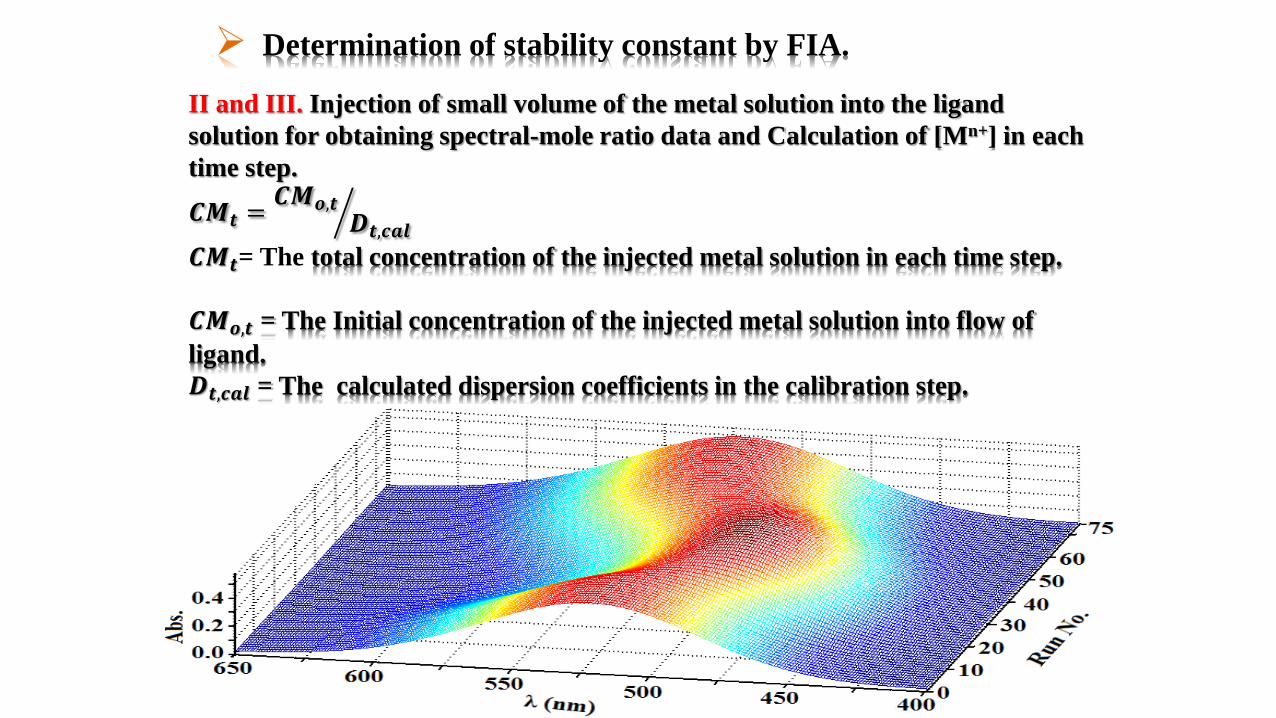
II and III. Injection of small volume of the metal solution into the ligand
solution for obtaining spectral-mole ratio data and Calculation of [Mn+] in each
time step.
𝑪𝑴𝒕 = 𝑪𝑴𝒐,𝒕
𝑫𝒕,𝒄𝒂𝒍𝑪𝑴𝒕= The total concentration of the injected metal solution in each time step.
𝑪𝑴𝒐,𝒕 = The Initial concentration of the injected metal solution into flow of
ligand.
𝑫𝒕,𝒄𝒂𝒍 = The calculated dispersion coefficients in the calibration step.
Determination of stability constant by FIA.

𝑪𝑳𝒕 = ( 𝑨𝒕,𝑳
𝑨𝟎,𝑳) × 𝑪𝑳𝟎
𝑪𝑳𝒕: The concentration of the ligand in time t after blank solution injection.
𝑨𝒕,𝑳: 𝐓𝐡𝐞 𝐚𝐛𝐬𝐨𝐫𝐛𝐚𝐧𝐜𝐞 𝐨𝐟 𝐭𝐡𝐞 𝐥𝐢𝐠𝐚𝐧𝐝 𝐬𝐨𝐥𝐮𝐭𝐢𝐨𝐧 𝐚𝐭 𝐭𝐢𝐦𝐞 𝐭 𝐚𝐟𝐭𝐞𝐫 𝐭𝐡𝐞 𝐛𝐚𝐥𝐧𝐤 𝐬𝐨𝐥𝐮𝐭𝐢𝐨𝐧 𝐢𝐧𝐣𝐞𝐜𝐜𝐭𝐢𝐨𝐧.
𝑨𝟎,𝑳: The absorbance of the ligand solution when the injected blank solution has not reached to
the detector yet.
𝑪𝑳𝟎: 𝐓𝐡𝐞 𝐢𝐧𝐢𝐭𝐢𝐚𝐥 𝐜𝐨𝐧𝐜𝐞𝐧𝐭𝐫𝐚𝐭𝐢𝐨𝐧 𝐨𝐟 𝐭𝐡𝐞 𝐥𝐢𝐠𝐚𝐧𝐝 𝐬𝐨𝐥𝐮𝐭𝐢𝐨𝐧.
III and IV. Studying the effect of ligand dilution (Injection of the
blank solution into flowing ligand solution).
Determination of stability constant by FIA.

V. Calculation
Determination of stability constant by FIA.
The general formula resulting from mass-balance equations:
[𝑳]𝒏+𝟏𝜷𝒏 + [𝑳]𝒏 𝜷𝒏 𝒏𝑪𝒕,𝑴 − 𝑪𝒕,𝑳 + 𝜷𝒏−𝟏 + [𝑳]
𝐧−𝟏 𝜷𝒏−𝟏 𝒏 − 𝟏 𝑪𝒕,𝑴 − 𝑪𝒕,𝑳 + 𝜷𝒏−𝟏 +⋯− 𝑪𝒕,𝑳
[L] : The concentration of free ligand in each time step in reaction coil.
β : The stability constants.
Ct,M: The total concentration of metal at each time step in reaction coil.
Ct,L: The total concentration of ligand at each time step in reaction coil.
n: Stoichiometry of complexation.

The calculated stability constants by the proposed method and comparison with other methods

Application of molecular modeling in
chromatography
Explore the mechanism of
adsorption
Find a selective ligand for affinity chromatography
Optimize the process
parameter

The molecular model used to investigate the affinity adsorbant is composed of four parts which describe the four main components:
• support• spacer• ligand• analyte
The support, the spacer and the ligand arecovalently bound and can have electrostatic andvan derWaals interactions with the analyte.
Molecular model

The surface can be visualized by
• All atom model
• End groups and ligands
Supprot
81

1. Design an affinity ligand

Molecular docking
Rigid protein Water deleted
Predict a ligand which can bind strongly to key regions of
protein
Main drawback

Molecular dynamics simulation (MDs)
Computational cost
Time consuming process
Solvent effect
can be performed only for a few ligand–protein
Flexibility of protein and ligand

• This work involves the design of peptide ligand of human serumalbumin by molecular simulations, aiming at the development of anovel affinity chromatography matrix for HSA purification.
This strategy includes four steps:• (1) building peptide library by amino acids location,• (2) docking these peptides into the candidate pocket of the target
protein and evaluating the affinity of the peptides to the targetprotein by using a scoring function,
• (3) more validating the affinity between the selected peptide ligandand the target protein by MD simulations.
• (4) a dipeptide of high affinity to HSA was found by the procedure. Itwas synthesized and its affinity to HSA was evaluated by UV-Visspectroscopy to ensure that this ligand has enough affinity for thepurification of HSA by affinity chromatography.

Ala-AlaAla-ArgAla-Asn
.
.
.Ala-TrpAla-TyrAla-Val
Ala-AlaArg-AlaAsn-Ala
.
.
.Trp-AlaTyr-AlaVal-Ala
Ala-TrpAla-tyrAla-PheAla-His
Trp-AlaPhe-AlaTyr-Ala
3 x 4 = 12
Peptid
e
Gold score
fitness
Peptide Gold score
fitness
Trp-Trp -70.667 Phe-
Phe
-62.425
Trp-Tyr -63.075 Phe-
His
-60.269
Trp-
Phe
-65.426 Tyr-Trp -65.665
Discovery Studio 2.5. GOLD program
P1
P2

ligand
spacer lys[ NH(CH2)6NH2] of ECH Sepharose 4B gel
Trp-Trp

• After the docking simulations, the complex of the candidate ligand and HSAwas further analyzed by MD simulations. The GROMACS3.3 simulation packagewas used to study the changes of the complex with time.• Water molecules can provide bridging interactions between the ligand andsome amino acid residues of the candidate pocket, and they are involved in thesolvation and desolvation processes in ligand binding.

a mathematical transformation employed to transform signals between time (or spatial) domain and frequency domain.

It is used to determine the frequency content of local sections of a signal as it changes over
time.
The function to be transformed is first multiplied by a window function, and the resulting
function is then transformed with a Fourier transform to derive the time-frequency analysis.
Wide windows do not provide good localization at high frequencies
Narrow windows do not provide good localization at low frequencies

Overcomes the preset resolution problem of the STFT by using a variable length window:
Use narrow windows at high frequencies for
better time resolution
Use wider windows at low frequencies for better frequency
resolution
Mother waveletsignal


Convolution is similar to cross-correlation.
convolution

A greater scaling factor is associated to a wider wavelet function and therefore
results in the low frequency components of the signal and vice versa. Therefore,
wavelet transform reveals the characteristic information of the signal at different
scales.

CWTof objects in class 1
Class 1
Class 2
CWTof objects in class 1
F-matrix
data matrix of samples F-ratio
thresholding
Best feature space
A careful search method using wavelet transform
S X L X NNXL
Toward applying CWT a fine multi-resolution space and characterization feature space is
provided. Indeed, CWT due to its redundancy property is able to provide such a finer multi-
resolution space that visualizes all information content of the signal.

DiscoTech
• A series of low-energy conformers for each molecule is computed.
• Each conformer of molecule is characterized byligand points and site points.
• Site points are the hypothetical position ofcomplementary atoms in the binding site and aredetermined from the position of heavy atoms in theligand structure.

• A clique detection algorithms used to align structures based on these distances.
• Each conformation of the reference molecule in turn is compared to all conformations of the other molecules.
• The cliques identified are examined to find one that is common to at least one conformation of every molecule.
• This process is repeated for every conformation of the reference molecule. If no solution is found the tolerances on the clique detection process are increased until either a solution is found or the maximum tolerance is reached.
• The output from a Disco run is a ranked list of all possible pharmacophoremappings

Gasp
Conformational analysis together with randomrotations and a random translation are appliedon the fly before any superimposition.
The chromosomes encode the angles of rotationof the rotatable bonds in all of the molecules andthe mapping of the pharmacophoric features inthe base molecule to corresponding features ineach of the other molecules.
A least-squares procedure is used to overlay eachmolecule onto the base molecule using themappings.
Fitness is calculated as a combination of the
similarity and the number of the overlaid features,
together with the volume integral of the overlay.

Case Study

Case Study• 32 2,4-dioxopyrimidine-1-carboxamides endowed
with acid ceramidase inhibitory activity; pIC50values
• Kennard and Stones (KS) algorithm was used tosplit the dataset (25 compounds were included intraining and 7 compounds in test set)
• Alignment was applied by Field-fit and DistillRigid body
• CoMFA and CoMSIA as 3D QSAR methods
• DiscoTech and GASP as pharmacophore modelbuilding methods

ResultsSummary of CoMFA and CoMSIA results based on two different alignment methods.
PLS statistics Distill alignment Field fit alignment
CoMFA CoMSIA CoMFA CoMSIA
R2cv 0.868 0.804 0.841 0.801
SEP 0.387 0.472 0.424 0.475
R2ncv 0.977 0.927 0.973 0.938
F-ratio 304.08 89.01 249.83 106.27
R2pred 0.899 0.844 0.727 0.846

Results
Result of pharmacophore hypothesis generated by DISCOtech and refined by GASP.
Model
No.
Fitness
score
Size Hits Dmean Features
1 3150.66 5 5 5.9044 DS1, AA1, HY1, AA2, DS2
2* 3399.37 5 5 5.9048 DS1, AA1, HY1, AA2, DS2
3 3364.77 5 5 5.9105 DS1, AA1, HY1, AA2, DS2
4 3286.6 5 5 5.8958 DS1, AA1, HY1, AA2, DS2
Size: total number of features in the models; Hits: number of molecules that matched during the search; Dmean: average inter-point distance
between the features; DS: donor site; AA: acceptor atom; HY: hydrophobic. *The best selected model.

Plots of the experimental versus predicted pIC50 values of 3D-QSAR from both CoMFA and CoMSIA for
the training and test compounds of Distill alignment + Steric contour map
4
5
6
7
8
9
4 5 6 7 8 9
Pre
dic
ted
pIC
50
va
lues
Experimental pIC50 values
CoMFA training compounds
CoMSIA training compounds
CoMFA test compounds
CoMSIA test compounds

Whole the samples in the
space (MLR, PLS, SVM,…)
Regression
Split the space and do local
regress on each sub region
(Decision trees,…)
112

Root or Parent node
Child /Parent node
Leaf or Terminal node
X1
X3X2
Split
Node
If-Then
Best- first
Up-Down
Left-Right
113
CART: Classification and Regression Tree
Binary recursive partitioning tree
• Binary
split parent node into two child nodes
• Recursive Partitioning
each child node can be treated as parent node
For example: X1 is the best variable

A ColdQuinsy
آماس لوزه ها
T<37
Influenza or
Pneumonia?
X3
Cough? Y /N
The
influenzaPneumonia
Cold or
Quinsy?
X 2
Throat?
Normal /Red
T>38.5
Classification ExampleY= {a cold, quinsy, The Influenza, Pneumonia, Healthy}
X1=temperature, X2 =a reddening throat, X3=coughing
1. If X1 < 37 , Y="is health“
2. If X1 ∈ [37, 38.5] and X2="there is reddening of throat", then Y="angina";
3. If X1 ∈ [37, 38.5] and X2="there is no reddening of throat", then Y="to catch cold";
4. If 38.5 >X1 and X2="there is cough", then Y="pneumonia";
5. If 38.5 >X1 and X2="there is no cough", then Y="influenza";
Health
PatientsX1
Temperature
[37.0, 38.5]

Temperature
Cough? Y /N
Throat? Normal /Red
Splitting Space to sub regions
Simulation of physician’s brain in decision

when the quality of a particular split falls below
the threshold, the tree is not grown further along
that branch. The tree is called fully grown tree.
Split-stopping
xp
••••••
•••••
•
y
Ῡr
Ῡl
•Split point
•
Split Criterion (regression):

Advantages of CART
It is nonparametric
Handle all types of variables: numeric, categorical
Immune to outliers
Computational is fast
"Off-the-shelf" procedure: Few tunable parameters
Interpretable model representation: Binary tree graphic
Disadvantages of CART
CART does not use combinations of variables
Tree structures may be unstable: a change in
the sample may give different trees
Low prediction accuracy

Ensemble, to maintain advantages
while increasing both accuracy and the
stability of classification and regression
trees.
Why Ensemble?
Ensemble Methods=
Committee methods =
Consensus methods=
Fusion methods

CART (Breiman, Friedman, Stone, Olshen,
1983)
Bagging (Breiman, 1996)
Random Forest (Ho, 1995; Breiman 2001)
Boosting
AdaBoost (Freund, Schapire, 1997)
Gradient Boosting (Friedman, 2001)
Stochastic Gradient Boosting (Friedman, 1999)
Ensemble methods
125
مثال موسیقی حاصل از جماعتی از
ک نوازندگان خبره زیباتر از یک ت
نوازنده است حتی اگر ساز خود را
خوب کوک کرده باشد
نمره دادن به یک سمینار 2مثال
ه بصورت خوب بد متوسط و یا نمر
دهی به ارائه دهنده توسط یک نمره
دهنده

p
all p variables
(Bagging: Bootstrap aggregating)
Aggregation of experts:
:البته برای رفع خستگی
Aggregation of experts: به فارسی میشه مجلس رو
ای خبرگان هم ترجمه کرد یعنی انصافا ما قبل از آمریکایی ه
این روش ها رو کشف 1357توسط اقای هاشمی و کنی در
کرده بودیم و در موضوع انتخاب رهبری از اونها استفاده
(البته تکبیر فراموش نشه). کرده بودیم

X Y
127
متغییرها را تصادفی انتخابCARTدر اینجا درخت
ییرها نمی کند بلکه در ریگراسیون اول یک سوم متغ
بطور تصادفی انتخاب می شوند بعد ازمیان انها
ر با توجه به متغییری که خطای کل دCARTدرخت
splitکردن را بیشتر کاهش می دهد را، انتخاب می
اجرا میشود CARTکند یعنی همان الگوریتم
CART درRF از نوعunpruned است

128
مثال پیرمردی که به هر فرزند یک
چوب داد و فرزندان را نصیحت می
نند کرد که یک چوب ضعیف رابشک
.کردboostو بعد چوبها را

130
Adaboost R2 (regression):
• 1. Initially, to each training pattern we assign a weight, wi =1
• 2. Construct a regression machine t from that training set.
• 3. Pass every member of the training set through this machine to obtain a prediction
• 4. Calculate a loss for each training sample

131
5. Calculate an average loss:
6. Form β, confidence index:
7. Update the weights:
8. For a particular input xi, each of the T machines makes a prediction ht , t =1, ..., T. Obtain the cumulative prediction hf using the T predictors:Calculate the weighted median for each sample


Adaboost R3

139
Results of different tree based algorithms for crizotinib data set
RMSEC RMSEP Condition(s)
CART 0.2182 1.0271 Prune=On
Bagging 0.4771 0.6898 mtry=241, ntree=1000, node size=5
RF 0.4919 0.6600 mtry=80, ntree=1000, node size=5
Boosting (Adaboost R2)
0.4098 0.7104 Sq, ntree =100
241 variables; Sq: Squared Loss Function, ntree: Number of tree in ensemble, mtry: Number of used Variables
Dock (Accelrys)MIF (Pentacle Software) Duplex


