MULTIVARIATE STATISTICAL PROCESS CONTROL AND CASE-BASED REASONING FOR SITUATION ASSESSMENT OF SEQUENCING BARCH REACTORS Magda Liliana RUIZ ORDÓÑEZ ISBN: 978-84-691-6833-2 Dipòsit legal: GI-1299-2008
Transcript
MULTIVARIATE STATISTICAL PROCESS CONTROL AND CASE-BASED REASONING
FOR SITUATION ASSESSMENT OF SEQUENCING BARCH REACTORS
Universitat de GironaDepartament d’Enginyeria Electrica, Electronica i Automatica
Multivariate Statistical Process Control
and Case-Based Reasoning
for situation assessment
of Sequencing Batch Reactors
by
Magda Liliana Ruiz Ordonez
Advisor
Dr. Joan Colomer Llinas
DOCTORAL THESISGirona, SpainMarch, 2008
Universitat de GironaDepartament d’Enginyeria Electrica, Electronica i Automatica
Multivariate Statistical Process Control
and Case-Based Reasoning
for situation assessment
of Sequencing Batch Reactors
A dissertation presented in partialfulfillment of the requirements of the degreeof Doctor per la Universitat de Gironaen Tecnologies de la Informacio
By
Magda Liliana Ruiz Ordonez
Advisor
Dr. Joan Colomer Llinas
Girona, SpainMarch, 2008
Universitat de GironaDepartament d’Enginyeria Electrica, Electronica i Automatica
Abstract
Multivariate Statistical Process Controland Case-Based Reasoning for
situation assessment of Sequencing Batch Reactors
by Magda Liliana Ruiz Ordonez
Advisor: Dr. Joan Colomer Llinas
March, 2008Girona, Spain
This thesis focuses on the monitoring, fault detection and diagnosis of WastewaterTreatment Plants (WWTP), which are important fields of research for a wide range ofengineering disciplines.
The main objective is to evaluate and apply a novel artificial intelligent methodologybased on situation assessment for monitoring and diagnosis of Sequencing Batch Reac-tor(SBR) operation. To this end, Multivariate Statistical Process Control (MSPC) incombination with Case-Based Reasoning (CBR) methodology was developed, which wasevaluated on three different SBR (pilot and lab-scales) plants and validated on BSM1plant layout.
Results showed that, MPCA is a robust technique for monitoring and fault detectionof SBR operation. The MPCA was successfully tested for on-line (real-time) monitoringof pilot scale-SBR performing nitrogen removal - the first time this is achieved (to our bestknowledge). The MPCA methodology is now ready to be used as part of daily operationof the SBRs.
For the diagnosis part, a comprehensive evaluation of the CBR methodology for au-tomatic diagnosis of SBR process operation (BIOMATH and LEQUIA) was performed -the first time an artificial intelligent method applied within WWTPs. The methodologywas then tested on the BSM1 plant layout which were used to construct abnormal events,e.g. faults, sensor failures, etc. The CBR method used input from the MPCA (ratherthan raw process data) and the best descriptors for the assessment of the situation (cases)were found to be principal components and errors (Q) of the statistical model. The mainresults showed that the CBR successfully diagnosed a wide range of operational problems
vi
such as sludge bulking, influent inhibition/toxicity, high influent flow and sensor faults.The diagnosis performance of CBR method using several statistical extensions such asMPCA, Dynamic PCA and PCA were also studied. This comparison showed that theMPCA + CBR combination has a good diagnosis performance. However, a more theoret-ical and in-depth study of which inputs and descriptors to use for the situation assessmentstep in the CBR are needed to further improve the diagnosis.
In addition, the ability of CBR to maintain and update the knowledge was also stud-ied and tested successfully using DROP and IB family of algorithms. This showed thatrepeating the cycle of learning helps maintaining and updating the case-base of the CBR.
Overall, this adaptive and intelligent aspects of the method makes it a good candidatefor helping the management in the daily plant operation as an automatic diagnosis andreal-time warning tool. Such artificial intelligent methods are promising tools which hasthe potential to contribute to good management and operation of plants. Further re-search is, however, needed to improve and consolidate the application of CBR to WWTPoperations, including input descriptors, retrieve and update algorithms and decision mak-ing rules. All in all, this is expected to save operational costs as well as improve plantperformance to comply with the goals of urban water management.
El futuro empieza hoyy lo que actualmente se esta investigando
condicionara nuestra vida en un manana muy proximoJosep M. Orta
ToLucho
and Esteban
Acknowledgments
This doctoral thesis is the result of not only my own efforts, but also those of many peoplewho directly or indirectly have collaborated with me. However, with limited time andafter four years it is very difficult to remember all of them. Therefore, I apologize inadvance for not including in these lines some additional people who really deserve recog-nition.
First of all, I would like to express my gratitude to Dr. Joan Colomer Llinas, whosince the beginning trusted my responsibility, knowledge and abilities to participate inthe project DPI2002-04579-C02-01. His patience helped me to understand how to expressideas when writing reports, papers, etc. He also knew when I needed support to be ableto continue in my research.
I would like to thank Professor Dr. ir. Peter A. Vanrolleghem from Ghent University,who hosted me in his research group, giving me the opportunity to use his facilities andlaboratories. Furthermore, his group’s guidance, comments and suggestions helped me toturn some ideas into reality.
I thank Doctor Christian Rosen and Doctor Ulf Jeppsson from Lund University forproviding information, experience and data, as well as for all their attention when I wasworking within the Lund group.
I thank Dr. Jesus Colprim and Dr. Ma. Dolors Balaguer who provided information,experience, optimism and guidance to this doctoral thesis.
I thank Drs. Joaquim Comas and Ignasi Rodriguez, researches from the LEQUIAGroup who contributed with knowledge, experience and suggestions.
I thank Dr. Joaquim Melendez who contributed with suggestions.
I thank Dr. Gurkan Sin from the Technical University of Denmark who among laughsand meetings gave me important suggestions and ideas, and of course his friendship.
I thank the Spanish government through the coordinated research project Develop-ment of a system of control and supervision applied to a Sequencing Batch Reactor (SBR)for the elimination of organic matter, nitrogen and phosphorus DPI2002-04579-C02-01which has given me economical support during the period of the research scholarship“BES-2003-1931”.
xi
xii
I thank the Spanish government for economical support during my research visits tothe BIOMATH group at Ghent University and the Department of Industrial ElectricalEngineering and Automation at Lund University.
I thank Drs Gabriel Ordonez, Gilberto Carrillo, Roberto Martınez, Jaime Barrero,Gabriel Plata and Oscar Gualdron, professors and guides during my engineering studiesat the Industrial University of Santander (UIS) in Colombia, who motivated me to startmy PhD studies.
I thank the members of the eXiT research group (those who are always here, those whoare finishing, as well as those who are starting) for their friendship and support duringthis time.
I thank the BIOMATH and LEQUIA groups and the IEA Department who cooperatedwith information and comments.
I thank my family in Girona which is growing more and more: My brothers Ronald,Alvarito and Sebastian, my sister-in-law Sabik, my nephew Alejandro and niece Violeta,and my cousins Andrea, Dayan and Camilo, who have made me feel close to Colombia.
I thank my family in Colombia: My father Alvaro and my mother Amanda, who froma distance always encouraged me to keep jumping over obstacles in life.
I thank my cousin Jennifer from the USA, whom I have recently known as a friend.
I thank my friends Claudia, Cesar, Maria, Juan, Daniel, Fabiana, Guillermo, Maira,Martha, Rodolfo, David, Rosa, Javier, Vicky and Sonia who have been my family inGirona.
I thank Xavi, who has helped me in my work when I thought I would give up.
I thank life for giving me the opportunity to know lovely countries, wonderful people,amazing cultures, exciting history and enriching experiences.
Last but not least, thanks to my husband, Lucho, for being there when I have needed afriend and partner in my life. As a fellow PhD he gave me invaluable suggestions. Thanksalso to my son, Esteban, who is my inspiration to improve day by day.
Notation and Abbreviations
Notation
A Instances of the same classNearest neighbor
b Number of successful classifications in number of attemptsC Carboncα Standar deviation to a given αE Residual matrixh Number of instances stored in the data baseI Number of batchesJ Number of variablesK Number of samplesλ Eigenvaluem Number of variables in a data seriesN Number of principal componentsn Number of variables in a data seriesP Loading matrixpj Loading vectorsQ Loading Y matrixS Covariance matrixSI Set of instancessi one instanceQ Q-statistics
SPE-squared prediction errorT Score matrixtj Score vectorsTI Training instancesT 2 Hotelling T 2 statistics
D-statisticσ Standard deviationσ2 Varianceθ Sum of eigenvaluesµ MeanV Variance capturedX Historical data matrix of process variables
2D Two-dimensional data array3D Three-dimensional data arrayAOC Abnormal Operation ConditionAS Auto scalingASM1 Activated Sludge Model No1BIOMATH Department of Applied Mathematics, Biometrics and
Process ControlBSM1 Benchmark Simulation Model No1BSM1 LT Benchmark Simulation Model No1 long-termCA Cluster AnalysisCB Case BaseCBR Case-Based ReasoningCS Continuous ScalingCUSUM Cumulative SumDA Discriminant AnalysisDPCA Dynamic Principal Component AnalysisDO Dissolved OxygenDROP Decremental Reduction Optimization ProcedureICA Independent Component AnalysisED Equipment DefectsEF Electrical FaultEU European UnionEWMA Exponentially Weighted Moving-Average CharteXiT Enginyeria de Control y Sistemas InteligentesGS Group ScalingIB Instance-Based LearningILC Influence Load ChangeIAWQ International Association on Water QualityIWA International Water AssociationKLA Mass transfer coefficientKPCA Kernel Principal Component AnalysisLEQUIA Laboratorio de Ingenierıa Quımica y AmbientalMATLAB Matrix LaboratoryMBPCA Multi-Block Principal Component AnalysisMPCA Multiway Principal Component AnalysisMPPCA Multi-Phase Principal Component AnalysisMSPCA Multi-Scale Principal Component Analysis
xv
MSPC Multivariate Statistical Process ControlMOPs Memory Organization PacketsN NitrogenNH+
4 AmmoniumNIPALS Non-linear Iterative Partial Least SquaresNN Neural NetworkNOC Normal Operation ConditionNOx Nitrogen dioxideORP Oxidation Reduction PotentialP PhosphorusPC Principal ComponentPCA Principal Component AnalysispH pondus HydrogeniumPLS Partial Least Square
Projection to Latent StructuresSBR Sequencing Batch ReactorSNO Nitrate and nitrite nitrogenSNH NH+
4 + NH3 nitrogenSPC Statistical Process ControlSSR Solid State RelaysSVD Singular Values DecompositionTSS Total Suspended SolidsVC Variation in the CompositionWWTP Wastewater Treatment Plant
2.2.1 Semi-Industrial SBR Pilot Plant at University of Girona (LEQUIA) 142.2.2 Lab-Scale Plant SBR at University of Girona (LEQUIA) . . . . . . 172.2.3 Lab-Scale Plant SBR at Ghent University (BIOMATH) . . . . . . . 22
configuration: mixed tank 1, tank 2 and tanks 3, 4 and 5 aerated . . . . . 122.3 a) Semi-industrial Pilot Plant b) Operational Schema of the semi-industrial
3.1 Classification of monitoring, fault detection and diagnostic algorithms . . . 253.2 An illustration of the Shewhart chart. The rhombuses are observations.
The process is said to be ’in control’ . . . . . . . . . . . . . . . . . . . . . 293.3 Multivariate statistical analysis vs. univariate statistical analysis and a
comparison of the in-control status regions using T 2 . . . . . . . . . . . . . 303.4 Projection of the process variables in a new space using PCA . . . . . . . . 323.5 NIPALS algorithm . . . . . . . . . . . . . . . . . . . . . . . . . . . . . . . 343.6 Q-statistic and D-statistic with 95.27% confidence limits . . . . . . . . . . 393.7 Arrangement of a three-way array . . . . . . . . . . . . . . . . . . . . . . . 403.8 Decomposition of a three-way data array, X, by MPCA . . . . . . . . . . . 423.9 Other decomposition of a three-way data array, X, by MPCA . . . . . . . 42
4.1 CBR cycle . . . . . . . . . . . . . . . . . . . . . . . . . . . . . . . . . . . 474.2 The distance between the new case or new problem and cases A and B.
X1 and X2 are the characteristics that define the cases. . . . . . . . . . . 484.3 a)Central cluster instance b)Non-noisy border point c)Collection of border
5.1 Score plot for batches. Dashed line is the model . . . . . . . . . . . . . . . 605.2 DO (green line) and ORP (blue line) profiles when an EF occurs . . . . . . 605.3 ORP and DO profiles when and VC fault condition is presented a) NOC
b) AOC . . . . . . . . . . . . . . . . . . . . . . . . . . . . . . . . . . . . . 615.4 ORP and DO profiles when and ED fault occurs . . . . . . . . . . . . . . . 615.5 ORP and DO profiles in presence of rainwater . . . . . . . . . . . . . . . . 625.6 ORP and DO profiles a)Good final quality b)Normal final quality . . . . . 625.7 Types of events . . . . . . . . . . . . . . . . . . . . . . . . . . . . . . . . . 635.8 Q-statistics and T 2-statistics with 92.79% confidence limits for the Semi-
Industrial Pilot Plant . . . . . . . . . . . . . . . . . . . . . . . . . . . . . . 655.9 MPCA Methodology applied to pilot-scale SBR . . . . . . . . . . . . . . . 675.10 Scale process for variable wise models . . . . . . . . . . . . . . . . . . . . . 695.11 The Q-Q distribution of the first principal component for models that are
unfolded variable wise (left) and batch wise (right) and scaled with a) CSb) GS and c) AS approaches . . . . . . . . . . . . . . . . . . . . . . . . . . 71
6.1 Names for each developed CBR . . . . . . . . . . . . . . . . . . . . . . . . 946.2 Specificity and sensitivity of each control charts . . . . . . . . . . . . . . . 956.3 Specificity and sensitivity for Case Base 1 (CB1) . . . . . . . . . . . . . . . 966.4 Sensitivity for Case Base 2 (CB2) . . . . . . . . . . . . . . . . . . . . . . . 966.5 Division of the first data set . . . . . . . . . . . . . . . . . . . . . . . . . . 996.6 Assignment of class numbers for each event . . . . . . . . . . . . . . . . . . 1006.7 Names for each methodology developed . . . . . . . . . . . . . . . . . . . . 1006.8 Names for each test developed . . . . . . . . . . . . . . . . . . . . . . . . . 105
A.1 LAMDA-descriptors used to define batches . . . . . . . . . . . . . . . . . . 122A.2 Classes obtained by SALSA-LAMDA for semi-industrial pilot plant . . . . 125A.3 Batch class composition according to principal component . . . . . . . . . 125A.4 Classes from SALSA-LAMDA for BIOMATH SBR pilot plant . . . . . . . 126A.5 Names for classes of the first classification . . . . . . . . . . . . . . . . . . 129A.6 Names for classes of the second classification . . . . . . . . . . . . . . . . . 129
xxv
Chapter 1
Introduction
1.1 Legal framework
The treatment of wastewater has become one of the important environmental topics.Wastewater treatment is an important part of maintaining the highest possible quality ofnatural water resources (rivers, lakes and seas). With new regulations for quality mon-itoring of WasteWater Treatment Plants (WWTP) under directive 98/15/CE (Directiva98/15/CE de la Comision, de 27 de febrero de 1998, por la que se modifica la Direc-tiva 91/271/CEE del Consejo en relacion con determinados requisitos establecidos en suanexo I n.d.), it is necessary to introduce new technology for control and supervision.The objective is to harmonize urban wastewater treatment legislation throughout the Eu-ropean Union (EU), in an attempt to protect the environment from any adverse effects.If the treatment of wastewater is insufficient in one member state of the EU, it ofteninfluences other members, affecting human integrity (de los Diputados de Espana 1978).The treatment of urban water must vary according to the receiving waters, which can bemore sensitive or less sensitive, so the requirements for discharges from urban wastewatertreatment plants are different (CEE 1991). In this way, legislations minimize the adverseeffects on the environment of this discharges.
1.2 Project framework
Title:Development of an Intelligent Control System applied to a Sequenc-ing Batch Reactor (SBR) for the removal of Organic Matter, Nitrogen andPhosphorous. SICOTIN-SBR2
This project is a continuation of a previous project DPI2002-04579 whose promisingresults prompted the consideration of a more ambitious control system. Goals are to im-prove the overall process performance and adapt it according to the influent wastewatercharacteristics in a wastewater treatment plant.
In the previous project, a system of Case-Based Reasoning (CBR) was elaborated.This system is qualified to identify the situation of the process when finalizing a cycle,
1
2 1. Introduction
as well as to recover historical cases of operation in order to propose modifications tothe current operation conditions of the process. First, qualitative trends were used todepict tendencies of the process in order to obtain variables profiles. Second, the caseswere stored in a case-base. Finally, a comparison between the recovered historical casesand the diagnosis was developed (Rubio et al. 2004). In addition, due to the amount ofcollected data, a brief application of Multivariate Statistical Control technique was madewith promising results.
The results using Multivariate Statistical Control suggest the continuation of this lineof research in pursuit of other objectives, such as estimation of the characteristics of in-fluent water and the quality of effluent water. The nature of the process (by batches,nonlinear, highly variable in time) and a complete system of data acquisition and storageindicates suitable tools for CBR, (with an initial version already implemented) Multi-variate Statistical Process Control (MSPC), and a combination of both.
In this manner in this project, the use of CBR and MSPC is proposed to diagnose thestate of the process and to consider the characteristics of influent and effluent water.
1.3 Objectives
In this thesis, the monitoring and diagnosis of WWTP are investigated. The main ob-jective is to develop a methodology to assess Sequencing Batch Reactors (SBR) WWTP,focusing on Statistical Models and diagnosis using MSPC and CBR. The evaluation in-cludes determining whether abnormal operation is present and defining the fault class andits features. More specifically, the objectives of this work are the following:
To develop a methodology to detect and diagnose Normal and AbnormalOperation Condition (AOC) using historical data from several WastewaterTreatment Plants. The information will be processed in order to obtain parametersthat determine the real situation into the processes. This methodology could be used inthe future for situation assessment in full-scale plant.
To introduce a Multivariate Statistical Process Control (MSPC) approachin a Sequencing Batch Reactor plant for on-line monitoring. Since the processhas many sensors measuring variables for a long time, and since these data are highlycorrelated, Principal Component Analysis (PCA) and its extensions are proposed for re-ducing the dimensionality of the problem. Combined with other techniques, this will helpimprove and accelerate the monitoring and diagnostic processes.
To include Case Based Reasoning (CBR) to improve the results obtained fromthe MSPC methodology. CBR is an expert system which applies the experience andknowledge from experts about past situations. This experience can often provide a solu-tion to new problems to help operators in their daily management and operation of theplant.
1.4. Contributions 3
To validate the developed methodology in several processes with differ-ent kind of operating condition Since the main objective is situation assessment ofWWTPs, several plants with different types of problems and several operation conditionare considered in order to refine and improve the best methodology with the ability fordetermining the situations in whatever kind of SBR process.
1.4 Contributions
The main contributions presented in this work are the following:
• Mainly, this doctoral thesis makes a rigorous evaluation and testing of MultiwayPCA (MPCA) + CBR approaches on several systems with different scales allowinga realistic assessment of the methods and their feasibility to practice.
• A new approach to situation assessment to detect the abnormal behavior in Wastew-ater Treatment Plants is proposed. This approach uses MSPC and CBR. MSPC isused to reduce the dimensionality and to remove non-linearity in the data. CBR isused to build the Case-base to diagnose future events. Maintenance and updatingare made through the learning capacity of this tool.
• Several combinations of the above approaches are performed using two pilot plants,one semiindustrial pilot plant and one Benchmark simulation model. These pro-cesses have differences between them, for instance influent, size of reactors, prob-lems and operating conditions. The influent for the first two plants are prepared inthe laboratory with several ingredients (syntectic influent). In semi-industrial pilotplant the influent is taken directly from the real wastewater treatment plant whichmainly comes from residential area. In this aspect, a rigorous evaluation and testingof the methodology using various systems with different scales have been performed.This means that it should be possible to generalise the obtained results.
• Several options of data scale before building the model using MSPC are studied inorder to find the best option for this kind of process.
• A full implementation of the CBR approach for a WWTP is performed includingcase base building, maintenance and updating and on line application.
• The MPCA methodology in a WWTP is implemented on-line. A new module for theapplication of the proposed methodology has been added to the existent monitoringsystems.
• A combination of the MSPC with the LAMDA algorithm (monitoring + clustering)to situation assessment in WWTPs is performed to identify normal data and toclassify situations.
4 1. Introduction
1.5 Outline
The structure of the thesis consists of six chapters and two appendices where supplemen-tary materials are provided.
In the present Chapter (Chapter 1), the background, the general context and theproblem statement of the research carried out in this thesis is provided. Next the researchobjectives are outlined, which guide the research carried out throughout the thesis. Last,the structure of the book is given.
Chapter 2 provides a general description of the wastewater treatment systems usedthroughout the thesis to test and develop the MPCA and CBR methodology. In total,four different systems were used. The first one is the semi-industrial SBR pilot which per-forms nitrogen and organic matter removal. The second one is a lab-scale SBR performingnitrogen and organic matter removal. Both of these plants were hosted and operated inthe laboratory of LEQUIA research group (University of Girona, Catalonia, Spain). Thethird one is a lab-scale SBR that performs biological nitrogen, organic matter and phos-phorus removal hosted and operated in the laboratory of BIOMATH (Ghent University,Belgium). The last one, is the BSM1 benchmark plant layout which is developed by TaskGroup on Benchmarking of Control Strategies for WWTPs.
Chapter 3 presents a review of multivariate statistical methods used mainly for pro-cess monitoring purposes. To this end, the classification of monitoring, fault detectionand diagnoses algorithms and a state-of-the-art in the PCA applications are provided.Basic concepts and various methodologies developed within the context of univariate andmultivariate statistical process control are introduced. Special attention is given to multi-way principal component analysis with the possible unfolding and control charts for batchmonitoring process are explained.
Chapter 4 provides the theoretical background of the case-base reasoning (CBR) cy-cle. The four fundamental R’s of the CBR that is retrieve, reuse, revise and retain, areexplained. The artificial intelligence capacity of the approach to adapt and learn usingdecremental reduction optimization procedure (DROP) and instance-based learning (IB)algorithms are explained in detail. The detailed introduction of the DROP family ofalgorithms was felt necessary since it is the first time (to our best knowledge) a full imple-mentation of case-based reasoning (CBR) methodology to wastewater treatment plant isdone. In the same way, IB is also explained indepth, which ensures a continuous updateof the case-base.
Chapter 5 provides results from the evaluation of the MPCA methodology at two SBRsystems (semi-industrial pilot plant at LEQUIA group and lab-scale BIOMATH SBR).First, a preliminary work was performed using the data from the semi-industrial plant.Due to the correlation performed with the variables by means of the statistical model,several types of situations could be determined. Second, an indepth analysis of the appli-cation of MPCA to lab-scale SBR was done. The research in this section was done in adidactic sense to help find out how to build good MPCA models for process monitoring
1.6. Publications 5
purposes. In this regard, issues such as type of scaling and unfolding, number of principalcomponents were investigated in view of their impact on process monitoring performance.Finally, implementation of the MPCA for on-line monitoring of the semi-industrial pilotplant (at LEQUIA group) were performed and the results were given.
Chapter 6 describes results from the evaluation of the methodology combining CBRwith the MPCA approach. Three historical data were used for the evaluation: lab-scale BIOMATH SBR, COST/IWA simulation benchmark and lab-scale LEQUIA SBR.The development and evaluation of the methodology was carried in two parts. In Partone, the descriptors, the building of case-base and the retrieve algorithms of the CBRmethodology were addressed. This evaluation was performed using historical data fromlab-scale BIOMATH SBR plant. The objective was to find the best combination of de-scriptors, the retrieve procedure and the case-base structure. Having found that, the CBRmethodology was tested/validated using COST/IWA simulation benchmark generated setof operational data. In part two, the maintenance and updating algorithms of the CBRmethod were investigated using the data from lab-scale LEQUIA SBR. In this way, theCBR ability to delete redundant information and learn automatically were added.
Finally, the main conclusions obtained from the research results as well as recom-mendations for future work are described in Chapter 7. Additionally, results from thecombination of the LAMDA algorithm with the MPCA methodology are given in theAppendix A.
1.6 Publications
The following articles were published from the research results generated in this thesisstudy. The contribution of the author has been mainly to develop the MPCA and CBRalgorithms and the analysis and interpretation of results.
Book chapters
Ruiz M., Colomer J. and Melendez J. (2006) ”Monitoring a sequencing batch reac-tor for the treatment of wastewater by a combination of multivariate statistical processcontrol and classification technique”. Frontiers in Statistical Quality Control ISBN 103-7908-1686-8 Physica-Verlag Heidelberg New York.
Contribution: MPCA modeling, analysis, interpretation and writing.
International Journal Publications
Mujica L, Vehı J., Ruiz M., Verleysen M., Staszewski W. and Worden K. (2008)”Multivariate Statistics Process Control for Dimensionality Reduction in Structural As-sessment” Mechanical Systems and Signal Processing, 22:155-171.
Contribution: MPCA analysis and interpretation of preliminaries results.
6 1. Introduction
Ruiz M., Villez K., Sin G., Colomer J., Rosen C. and Vanrrolleghem P.A. (2008) ”Dif-ferent PCA approaches for monitoring nutrient removing batch process:Pros and Cons”in preparation for publication in Water Science and Technology.
Contribution: MPCA modeling, analysis, interpretation and writing.
Ruiz M., Sin G., Colprim J. and Colomer J., ”MPCA and CBR methodology for moni-toring, fault detection and diagnosis in wastewater treatment plant” (2008) in preparationfor publication in Water Science and Technology.
Contribution: MPCA modeling, CBR algorithms, analysis, interpretation and writing.
National Journal Publications
Ruiz M., Colomer J. and Melendez Q. (2006) ”Combination of statistical process con-trol (SPC) methods and classification strategies for situation assessment of batch process”Revista Iberoamericana de Inteligencia Artificial. 29:99-107.
Contribution: MPCA modeling, analysis, interpretation and writing.
International Conferences
Villez K., Ruiz M., Sin G., Rosen C., Colomer J. and Vanrrolleghem P.A. (2007) ”Com-bining Multiway Principal Component Analysis (MPCA) and clustering for efficient datamining of historical data sets of SBR processes” Proceedings of the 3rd InternationalIWA Conference on Automation in Water Quality Monitoring (AutMoNet2007), Ghent,Belgium, September 5-7, 2007, appeared on CD-ROM.
Contribution: Preliminary LAMDA methodology.
Ruiz M., Rosen C. and Colomer J. (2007) ”Diagnosis of a continuous treatment plantusing Statistical Models and Case-Based Reasoning”, Proceedings of the 3rd InternationalIWA Conference on Automation in Water Quality Monitoring (AutMoNet2007), Ghent,Belgium, September 5-7, 2007, appeared on CD-ROM.
Contribution: Modeling and diagnosis analysis using PCA, DPCA, MPCA and CBR,interpretation and writing.
Jaramillo M., Ruiz M., Colomer J. and Melendez J. (2007) ”Multiway Principal Com-ponent Analysis and Case Base Reasoning methodology for abnormal situation detectionin a Nutrient Removing SBR” Proceedings of the European Control Conference, Kos,Greece, July 2-5, 2007, appeared on CD-ROM.
Contribution: Modeling and diagnosis analysis using MPCA and CBR, interpretationand writing.
1.6. Publications 7
Ruiz M., Villez K., Sin G., Colomer J. and Vanrolleghem P.A. (2006) ”Influence ofscaling and unfolding in PCA based monitoring of nutrient removing batch process” 6thIFAC Symposium on Fault Detection, Supervision and Safety of Technical Processes.September, 2006, Beijing P.R. China.
Contribution: MPCA modeling, analysis, interpretation and writing.
Ruiz M., Colomer J., Rubio M., Melendez J. and Colprim J. (2004) ”Situation as-sessment of a sequencing batch reactor using multiblock MPCA and fuzzy classification”BESAI Worshop in Binding Environmental sciences and Artificial Intelligence, ECAI 2004European Conference on Artificial Intelligence, ISSN.0922-6389, August, 2004, Valencia(Spain).
Ruiz M., Colomer J., Colprim J. and Melendez J. (2004) ”Multivariable statisticalprocess control to situation assessment of a sequencing batch reactor”, CONTROL 2004,pp.11, ISBN.0 86197 130 2, September, 2004, Bath (UK).
Contribution: MPCA modeling, analysis, interpretation and writing.
Ruiz M., Colomer J., Rubio M. and Melendez J. (2004) ”Combination of multivari-ate statistical process control and classification tool for situation assessment applied toa sequencing batch reactor wastewater treatment” ISQC Intelligent Statistical QualityControl pp.257-267. ISBN.83-88311-69-7. June, 2004, Warszawa (Poland).
Ruiz M., Melendez J., Colomer J., Sanchez J. and Castro M. (2004) ”Fault locationin electrical distribution systems using PLS and NN” Proceedings of the InternationalConference on Renewable Energies and Power Quality (ICREPQ’04), Barcelona, Spain,2004, appeared on CD-ROM.
Contribution: PLS modeling, NN classification, analysis, interpretation and writing.
Chapter 2
Wastewater Treatment Plants
Every community produces solid and liquid wastes. Liquid waste refers to water afterof residential, industrial and commercial sectors usage (wastewater). If it is accumulatedand stagnated bad-smelling gases are generated, including a big number of human harmfulmicroorganisms. Also, it includes nutrients favoring the growth of aquatic plants whichcontain toxic compounds. To prevent this situation, the European Union has regulated thefinal quality of urban wastewater with the new directive 98/15/CE (Directiva 98/15/CEde la Comision, de 27 de febrero de 1998, por la que se modifica la Directiva 91/271/CEEdel Consejo en relacion con determinados requisitos establecidos en su anexo I n.d.). Themain objective is to protect the environment from the negatives effects of this wastewater.As a consequence, the biological nutrient removal technology has been increased aroundthe world in WWTPs (Figure 2.1).
Figure 2.1: Wastewater system
9
10 2. Wastewater Treatment Plants
Extracted from Benchmark-Web 2007
In an Activated Sludge (AS) process, the most commonly used technology for mu-nicipal wastewater treatment is the biomass. This is composed of a wide mixed cultureof microorganisms is blended with the wastewater, which is composed of organic matter,suspended solids and nutrients. The mixture is then discharged to another reactor whichis typically a settling tank to separate the biomass from the treated water.
2.1 The continuous process
Treatment plants perform primary treatment (physical removal of floatable and settleablesolids) and secondary treatment (biological removal of dissolved solids).
Primary treatment involves (Federation 2003):
1. Screening - to remove large objects such as stones or sticks, which could plug linesor block tank inlets.
2. Grit chamber - slows down the flow to allow grit to fall out.
3. Sedimentation tank (settling tank or clarifier) - settleable solids settle out and arepumped away, while oils float to the top and are skimmed off.
Secondary treatment consists of a biological conversion of dissolved and colloidal or-ganic compounds into stabilized, low-energy compounds and new biomass cells, caused bya very diversified group of microorganisms that respire in the presence of oxygen. Threeoptions are explained below (Comas 2000):
1. Activated Sludge - The most common option uses microorganisms in the treatmentprocess to break down organic material with aeration and agitation. The mixtureis continually recirculated back to the aeration basin to increase the rate of organicdecomposition.
2. Trickling Filters - The wastewater is sprayed on stone or plastic beds, allowing itto trickle. Microorganisms growing on the beds break down organic material in thewastewater. Trickling filters drain at the bottom; the wastewater is collected andthen undergoes sedimentation.
3. Lagoons - These are slow, cheap, and relatively inefficient, but can be used forvarious types of wastewater. They rely on the interaction of sunlight, algae, mi-croorganisms, and oxygen (sometimes aerated).
In this thesis, the goal is to diagnose normal and abnormal operation condition inWWTPs. Two kinds of plants are considered, a COST/IWA simulation benchmark (Copp2002) and a Sequencing Batch Reactor (SBR) process. Each of these processes is explainedin the next sections.
2.1. The continuous process 11
2.1.1 The COST/IWA simulation Benchmark
The International Association on Water Quality (IAWQ) held a meeting in 1983 in whicha group was formed to promote and develop practical applications of models for the de-sign and operation of biological wastewater treatment systems (Jeppsson 2007). To date,several objectives have been developed. One is the COST/IWA simulation benchmarkwhich compares and evaluates different control strategies for a biological nitrogen re-moval process. In “benchmark simulation the goal is to obtain good performance andcost-effectiveness in wastewater management systems, given detailed descriptions of plantlayout, model parameters and simulation models. The benchmark simulation comparespast, present and future control strategies without reference to a particular facility col-lecting large amounts of data (Copp 2002).
The benchmark simulation system includes a plant layout, simulation models and pa-rameters, a detailed description of influent disturbances (dry weather, storm and rainevents), as well as performance evaluation criteria to determine the relative effectivenessof proposed control strategies (Copp 2002). The plant has five completely mixed reactorswith a total volume of 5999 m3 of which tanks 1 and 2 are each 1000 m3 and tanks 3,4and 5 are each 1333 m3 (see Figure 2.2a)). The biological process is modeled using theActivated Sludge Model No1 (ASM1) (Henze et al. 1987), and the settling processes aredescribed using the Takacs ten-layer model (Takacs et al. 1991). Several platforms havebeen used to develop for the Benchmark simulation using C/C++, Fortran and Simulink-MATLAB among others. In this thesis, the Simulink-MATLAB platform is used, seeFigure 2.2b).
The Benchmark Simulation Model No1 (BSM1) has seen continuous improvementsto the control system, procedure and evaluation criteria, however, it does not allow forLong-Term (LT) evaluation. To overcome this inconvenience, Rosen et al. (2004) andJeppsson et al. (2006) have proposed long-term monitoring strategies (BSM1 LT ) andanother extension to allow control strategy development and performance evaluation ata plant-wide level (BSM2). Among other changes in BSM1 LT , the toxic componentshave been characterized by their concentration and not as a percentage of toxicity.
The final version of BSM1 is still in evolution; in this work, the most recent pro-totype has been used in order to acquire data. This version is closest to reality and awell known benchmark plant for evaluating the methodology developed in this doctoralthesis. In total, 9 sensors were simulated to monitor the process; they are: flow rate,Nitrate and nitrite nitrogen (SNO), units gN m−3 : SNO reactor2, SNO reactor5;NH+
4 + NH3 nitrogen (SNH), units gN m−3: SNH reactor5; Total Suspended Solids(TSS), units mg/l: TSS reactor5, SNIT plantinput; Mass transfer coefficient(KLA),units m/s: KLA reactor3, KLA reactor4, KLA reactor5. 96 samples per variable werecollected. 609 days were simulated so that the dynamic influent data become steady state.The first 63 days are disregarded would become steady state. 364 days were used to iden-tify and train the statistical models and the CBR approach. Immediately afterwards, 182days were used to evaluate the monitoring models and diagnosis. The AS process is acomplex system with operational problems. One of these problems has been simulated:
12 2. Wastewater Treatment Plants
Figure 2.2: a)Simulation benchmark system b)Representation in the Simulink-MATLABconfiguration: mixed tank 1, tank 2 and tanks 3, 4 and 5 aerated
Filamentous bulking (Bulking event). A bulking event is mainly caused by low DO in theaeration tank, causing growth of filamentous bacteria. This makes the separation of thebiomass from the treated water difficult (bad settling). The events used in benchmarksimulation were the following:
• Training set (364 days): Two bulking events starting from day 30 to 46 and 329 to355. Five incidences of low level of inhibition however enough to affect the bacterialpopulation due to toxicity starting from day 72 to 76, day 92 to 94, day 154 to 155,day 261 to 263 and 285 to 295. 41 aleatory days with high flow rate event. Finally,Day 180 with nitrate sensor fault.
• Evaluating set (182 days): Bulking event starting from day 122 to 147. Two inci-dences of low level of inhibition, with a soluble carrier start in day 60 to 62, day 110to 112. Another inhibition/toxicity event with a particulate carrier is imposed day72. Finally, 21 aleatory days with high flow rate event
2.2. Sequencing Batch Reactor 13
2.2 Sequencing Batch Reactor
The main characteristic of the SBR is that whole process occurs in the same reactor fol-lowing a sequence of phases, while in a continuous wastewater process plant such as theBSM1 LT plant shown above each phase occurs in different reactors. The SBR processhas been shown to be an effective alternative to treat wastewater from domestic and in-dustrial waste.
The advantages of the SBR process can be attributed to:
1. Design:
• the clarification occurs in the same reactor.
• a portion of the treated water is replaced by untreated wastewater for eachcycle, distinguishing the SBR process from other continuous flowtype activatedsludge systems.
• influent and effluent flows are uncoupled by time sequencing.
2. Microbiology: Biological processing is cyclic.
3. Operation: The process operation can be easily adapted for different requirementsby changing the duration of each phase.
The operation in a SBR process is performed by means of repeating a defined cycle.This cycle has four basic phases:
1. Fill: The influent wastewater is pumped into the reactor to be treated. The reactorcan be filled under different conditions depending on operating conditions.
2. Reaction: Aerobic and anoxic conditions are combined in order for the biomass toconsume the substrate from the influent wastewater.
3. Settle: This phase occurs when the aerobic and anoxic conditions finish. Normally,this phase is quicker than in a continuous process. The excess sludge is drained.
4. Draw: When the process finishes, the treated water is drawn from the reactor. Inthis way, it is ready to start the process with new influent wastewater.
Filling and reaction phases can be combined and configured in different ways and sev-eral times. This combination depends on the main objective of the treatment, the organicmatter and nitrogen removal. The settle and draw phases are the last ones in the cyclestructure. The most common structure is based on a combination between anoxic andaerobic conditions ending with the settling and draw phases (Corominas. 2006).
The SBR plant carries out advanced treatment, in which the nitrogen is removed intwo steps as follows (Vives et al. 2001):
14 2. Wastewater Treatment Plants
Nitrification : Ammonia is converted to nitrate by aerobic nitrifying (autotrophic) mi-croorganisms.
Denitrification : Nitrate is converted to N2O or reduced to nitrogen gas under anoxic(without oxygen) conditions by anoxic heterotrophic microorganisms.
In this thesis, three SBR pilot plants have been used: two from the Laboratorio deIngenierıa Quımica y Ambiental (LEQUIA) and one from the Department of AppliedMathematics, Biometrics and Process Control (BIOMATH). The expert knowledge of theprocess is the interpretation of profiles of some state variables which will be used to decidespecial events into the processes. In SBR pilot plants from the LEQUIA, these variablesare Oxidation Reduction Potential (ORP) (mV), pondus Hydrogenium (pH), DissolvedOxygen (DO) (mg/L) and Temperature (C). In the BIOMATH pilot plant, the variablesare ORP, pH, DO, weight, conductivity and Temperature. These variables provide infor-mation about the biological reactions and the process state. The on-line measurements inthe settling and draw phases of the SBR are usually not consistent due to changing prop-erties/dynamics of settling in each batch (Sin et al. 2004) (Lee and Vanrolleghem 2003b).As a consequence, these phases are not considered in the development of the methodolo-gies.
2.2.1 Semi-Industrial SBR Pilot Plant at University of Girona(LEQUIA)
Generalities
The semi-industrial pilot plant is located at a real wastewater treatment plant in Spain(Catalonia), seen in Figure 2.3a. It is composed of a metal square reactor of 1m3. Theminimum and maximum volumes of the reactor are 483 liters and 683 liters respectively,and a volume of 200 liters of water to process (see Figures 2.3b and 2.4).
Figure 2.3: a) Semi-industrial Pilot Plant b) Operational Schema of the semi-industrialpilot plant SBR
2.2. Sequencing Batch Reactor 15
Figure 2.4: Operational schema of the semi-industrial pilot plant SBR
Wastewater is taken directly from the real WWTP by means of a peristaltic pump(Watson Marlow 621 F/R 77 RPM, flow=0−50L.h−1) after passing through a grit cham-ber, sand and grease removal units (see Figure 2.5) in order to be stored in a storage tankunder mixing conditions without refrigeration.
Figure 2.5: Storage tank Filling
Next, the wastewater is pumped to the reactor by means of another peristaltic pumpaccording to the operating conditions. During the reaction phase, the mixed liquor ismaintained under suspension and homogeneous conditions using a marine helix. The en-ergy provided for mixing is used to regulate the distribution of mixed liquor solids in thereactor. The aerobic condition is achieved by four air filters (SKS-80 EW) through porousdiffusers located at the bottom of the reactor. The air supply is controlled by an ON-OFF
16 2. Wastewater Treatment Plants
valve in order to achieve complete nitrification and avoid high DO concentration whenthe anoxic conditions start (Corominas. 2006).
The monitoring and control systems consist of three parts: acquisition, monitoringand control system. The SBR process is equipped with DO-Temperature (OXIMAX-WCOS 41), pH (CPF 81) and ORP (CPF 82) Endress-Hauser sensors. These signals arecaptured by a data acquisition card (PCI-6025E from National Instruments). The wholeprocess is controlled by software in LabWindows (from National Instruments). The con-trol is performed by a power relay output board (SC-2062 from National Instruments)(Puig et al. 2004).
Operating conditions and cycle description
The semi-industrial SBR pilot plant is run with a fixed cycle found by Vives (2004), whichoptimizes the cycle to achieve complete nitrification and denitrification. The duration ofoperation stages are fixed. Each cycle takes 8 hours and has 5760 samples (obtained every5 seconds) per variable. There are six anoxic-aerobic phases of reaction, with filling onlyoccurring during the anoxic condition. The applied operation stages are shown in Figure2.6. The cycle is divided into 395 minutes of reaction phase, with 46% of aerobic condi-tions and 54% of anoxic condition, 60 minutes of settling, and finally 25 minutes of draw.The reaction phase is divided into 212 minutes of anoxic conditions and 183 minutes ofaerobic conditions (Corominas. 2006).
Figure 2.6: Cycle applied to semi-industrial SBR pilot plant
Re-sampling and time warping
The plant ran continuously for 60 days. Each batch took 8 hours with 5760 samples foreach variable (one sample every 5 seconds). Due to computer limitations only 392 samplesper batch are used. To test whether the samples per variable could correctly determinethe operation of the process, the profile of each variable was studied. The profiles areimportant because they contain important points that provide valuable information aboutthe beginning and ending of the biological reactions. In this way, one sample for eachminute is considered. The 5760 and 392 time instants are contrasted in Figure 2.7, to
2.2. Sequencing Batch Reactor 17
verify that the variables profiles do not change. Settling and drawing have not been takeninto account because they are usually not consistent due to changing properties/dynamicsof settling in each batch (Sin et al. 2004) (Lee and Vanrolleghem 2003b).
In Figure 2.7, the first variable is ORP for both lengths, the normal range of values isaround −300mV in anoxic stages and 0 to 50mV in aerobic stages. In anoxic stages, thereis a bending-point called the nitrate knee. It occurs when the denitrification reaction hasfinished; this is perceived in both profiles. The third variable is pH, which has two im-portant points that provide information about the end of nitrification and denitrification.Comparing both profiles, it can be seen that the profiles are equal. This implies that theSBR biological process changes slowly.
2.2.2 Lab-Scale Plant SBR at University of Girona (LEQUIA)
Generalities
The lab-scale plant SBR is located at the University of Girona (Catalonia-Spain). Themaximum capacity of this SBR pilot plant is 30 liters, and the minimum operating ca-pacity is 20 liters (see Figure 2.8). This minimum capacity is the residual volume at theend of each SBR cycle. The influent wastewater is synthetic. It is a blend of carbonsource, an ammonium solution, a phosphate buffer, alkalinity control and microelementssolution. The influent wastewater is stored in a tank with a capacity of 150 liters. Thetemperature in the storage tank is 4OC to minimize microbial activity. The reactor oper-ates in a predefined cycle of fill, reaction, settle and draw modes. This reactor is locatedin a thermoregulated room at 20oC.
The influent wastewater is transferred from the storage tank to the reactor by meansof a peristaltic pump (Watson Marlow). Similar peristaltic pumps are used to fill, purgeand draw. The sludge and wastewater are mixed under homogeneous conditions. For thispurpose, a marine helix is used with a nominal value of 400 rpm. The reactor is operatedunder anoxic and aerobic conditions. Injecting compressed air creates aerobic conditions,without dissolved oxygen control. The compressed air is injected at the bottom of thereactor. The dissolved oxygen is controlled inside the reactor by means of an electrovalve.When the reaction has finished, the settling phase starts to separate the sludge fromthe treated water, decanting at the bottom of the reactor. Finally, the treated water isdischarged. To monitor essential variables the SBR process is equipped with DO (WTWOXI 340), Temperature (PT 100), pH (EPH-M10) and ORP (ORP M10) Endress-Hauserprobes. These sensors are connected directly to the control panel. The signal is processedby a data acquisition and control card PCI-821PG, afterwards sending a digital signal inorder to drive the power relay output board controlling the orders to fill, draw, mix andair supply for the process (PCLD-885). The whole process is controlled by software inLabWindows (from National Instruments). This program has a user-friendly user interfacewhich makes it easy to create and change operating cycles.
18 2. Wastewater Treatment Plants
Figure 2.7: Comparison of 5760 samples and 392 samples for variables
Operating conditions and cycle description
The duration of operation stages is fixed. Each cycle takes 8 hours, divided into reaction,settling and discharge. Two combinations of the anoxic and aerobic conditions are imple-mented in this Lab-Scale SBR Pilot Plant, in which the number of filling events, anoxicand aerobic conditions are alternated.
2.2. Sequencing Batch Reactor 19
Figure 2.8: Lab-scale plant from LEQUIA
• Period 1: Three reactions are configured. The first reaction phase is a combinationof anaerobic and aerobic conditions. The second reaction is a combination of anoxicand aerobic conditions and the third reaction is a different combination of anoxicand aerobic conditions. Filling only occurs at the beginning of each reaction phases(see Figure 2.9).
Figure 2.9: Period 1 cycle configuration
• Period 2: This period has only two reactions configured. The final combination ofanoxic and aerobic conditions is eliminated from period 1 configuration (see Figure2.10).
Re-sampling and time warping
The data sets from both periods are contained in text files, representing data retrievedfrom the wastewater treatment plant during 8 hours working time (duration of a com-plete cycle of treatment). At the beginning of these files are found several header lines
20 2. Wastewater Treatment Plants
Figure 2.10: Period 2 cycle configuration
including information related to the measured variables, and other information. Next tothese header lines, and lasting until the end of the file, are the measured values of thevariables with a sample time of 5 seconds. The number of data contained in each file is5760.
Taking into account the large number of samples in each file and that the variation ofthe treatment process does not occur suddenly, and in order to reduce the computationalload, it is necessary to reduce the number of samples.
Table 2.1: Work schedule configuration from LEQUIA Lab-Scale Plant SBR
At the same time, the obtained data present several operating plans that are shownin Figure 2.1, notated as 3A, 3B, 2A, 2B and 2C, where the numeric value representsthe number of cycles in the process, and the character distinguishes between the differenttime phases configurations in which the processes packed in the same group are divided.Of those divisions, the last 3 (Wastage, Settling and Drawing), will not be taken intoaccount since the information added is not very important in this study. The strategiesstudied to reduce the data are:
• Independent data treatment: Each working plan will be treated independent theothers, reducing the number of data samples to 1 sample per minute in every phaseused. The expression for this new sample value is noted below:
X =
∑Ni=1 xiN
(2.1)
2.2. Sequencing Batch Reactor 21
where:x : new sample obtained for the actual time period.X : sample value placed at position i for the actual time period.N : number of samples needed to form a minute of real time.
One minute of sampling is sufficient since the time constant of biological reactionsare in the order of hours hence one sample per minute is selected because this is themaximum value recommended by experts when dealing with biological processes.
• Grouped data treatment: The strategy consist of packing all working plans thatshare the same number of cycles into one single pack, so the number of samplestaken must be unified in order to analyze the data. Two options are analyzed.
1. Reduction to the minimum value: As in the independent data treatment, themaximum sample frequency allowed when working with biological processes is 1sample per minute. This criterion will be taken as a reference for the minimumlasting time value, and the values that are greater will be undersampled to thisvalue. As an example, if the different length of the anaerobic phase are taken(Figure 2.2), the number of samples that should be used is 150, so it is theminimum value.
Table 2.2: Three different lengths for anaerobic phase configuration
When reducing to the minimum value, it is assumed that processes with ashorter length are more critical than others that have a longer length. Alsoit is deduced that processes with a longer duration have a slower reaction; inorder to acquire the same amount of information as in the shorter processes,the sample time must be greater. The formula to compute the new samples ofthe data is the same as that shown in Equation 2.1, with the number of periodsneeded to have 1 minute of real time changed as follows:
N =Datafromphase
min(d1..., dk)(2.2)
where d is the length of the analyzed phase among the working plans that sharethe same number of cycles.
2. Reduction to the maximum value: This time the more critical processes arethose that have a longer length. Those that have a shorter length value must beartificially enlarged. Keeping in mind that all processes have the same sampletime (1 sample per minute), it has been decided to use the following strategy:
22 2. Wastewater Treatment Plants
– Compute the mean values of each time instant of those working plans thathave the maximum length.
– For each working plan take 1 sample per minute, using Equation 2.2.
– For processes that have a smaller length than the maximal value, add themean values of the time instants needed to reach the maximal value at theend of the new samples.
If the mean value is added when computing the data, these new values represent0, so the new mean will not be affected.
2.2.3 Lab-Scale Plant SBR at Ghent University (BIOMATH)
Generalities
This pilot plant is located at Ghent University in Belgium. The maximum capacity of thisSBR pilot plant is 64 liters in which synthetic sewage is used as influent wastewater whichmimics real pre-settled domestic wastewater (see Figures 2.11, 2.12). Detailed informationabut the synthetic influent wastewater characterization can be found in (Insel et al. 2006).
Figure 2.11: Lab-scale plant from BIOMATH
The system consists of a PC, an analog/digital interface card, sensors, transmitters andSolid State Relays (SSR). This system controls the on-off status of the parasitical pumps,air supply and mixer and the duration of each phase; it also has a friendly interface (Leeet al. 2005). The data acquisition, pump and valve control loops are programmed in the
2.2. Sequencing Batch Reactor 23
Figure 2.12: Operational scheme of the SBR
LabView platform. The sensors for pH, ORP, DO, temperature, weight and conductivityare connected to the individual sensors. These measurements are recorded every 1 min(360 time instants per cycle). The operating conditions are displayed on the computer,and the collected data is stored in a data log-file. The aeration is controlled by means ofan on-off valve (Insel et al. 2006).
Operating conditions and cycle description
The pilot-scale SBR operation consists of 6-hour cycles (i.e., 4 cycles per day). Thescheduling of phases, optimized in (Sin et al. 2004), is shown in Figure 2.13. The fillphase comprises minutes 1 to 60 of each cycle. In the reaction phase (minutes 61 to 270)the operation is switched 4 times between aerobic (20 minutes) and anoxic conditions(32.5 minutes). The last aerobic phase from 271 to 300 minutes is followed by the settlingphase (45 minutes) and a draw phase (15 minutes). The excess sludge is wasted at theend of the second aerobic phase for each cycle.
Figure 2.13: Cycle applied to lab-scale plant SBR
24 2. Wastewater Treatment Plants
Re-sampling and time warping
The measurements of pH, ORP, DO, temperature, weight and conductivity are recordedevery minute, resulting in 360 measurements per variable per cycle in one batch run.However, only the first 300 time instants of each batch run are used (Sin et al. 2004) (Leeand Vanrolleghem 2003b).
2.3 Conclusions
Wastewater treatment consists of the elimination of contaminants in the water. Thetreatment used depends on the type of process. The process can be structured into threemain blocks based on their nature: physical, chemical and biological. All three are basedon the separation of wastewater in two phases, one containing clean treated water andanother containing solids. In this work two kinds of plants were used: a benchmark sim-ulation plant with a continuous activated sludge process configuration (BSM1) and theother is sequential batch reactor (SBR) with three different scales and configurations (1semi-industrial pilot plant, 1 lab-scale for COD and N removal and 1 lab-scale for COD, Nand P removal). While in benchmark simulation the treatment occurs in several reactors,in SBR the whole process occurs in the same reactor following a sequence of phases. Themain goal in benchmark simulation is determine the best control strategies including aplant layout, simulation models and parameters, as well as a detailed description of theinfluent disturbances. The main goal in the SBR process is to combine the filling andreaction phases in different ways and several times. Depending on these combinations,the organic matter and nitrogen are removed.
In next chapters the characteristics, operating conditions and requirements associatedwith each one of the these plants will be described. Then, explanations about proposedtools to evaluate the performance of a methodology to detect and diagnose normal andabnormal operation condition are described. Several tests are developed in order to obtainthe best methodology.
Chapter 3
Multivariate Statistical ProcessControl
3.1 Preview
Many strategies for monitoring, fault detection and diagnosis are referenced in the bib-liography. According to Venkatasubramanian et al. (2003), fault diagnosis methods canbe classified in three general categories: quantitative model based methods, qualitativemodel based methods and process history based methods, as illustrated by Figure 3.1.
Figure 3.1: Classification of monitoring, fault detection and diagnostic algorithms
The solution proposed in this thesis falls into the category of process history basedmethods and specifically into the subgroups of statistical methods and expert systems (seeChapter 4). The history of statistics dates back to the Egyptians. where the pharaohsgathered information about the population and wealth. Later on, the Roman Empireimproved these techniques. They carried out a census of the population every five yearsand recorded births and deaths. In the Middle Ages, this practice was forgotten until itwas revisited by men such as Leonardo de Vinci, Nicholas Copernicus, Galileo, Neper,William Harvey, Sir Francis Bacon and Rene Descartes (Marte 2003). Between 1800
25
26 3. Multivariate Statistical Process Control
and 1820, two fundamental concepts were generated for Statistical Theory: Laplace andGauss developed the theory of probability and the least squares approximation method(Schuldt 1998). In the late nineteenth century, Sir Francis Gaston developed the Cor-relation Method which measures the relative influence of factors on variables, and it ledto the development of the coefficient of correlation by Karl Pearson. Other importantcultivators of Biometry Science, such as J. Pease Norton, R. H. Hooker and G. UdnyYule, carried out studies of the Measure of Relations.
Statistical process control (SPC) began with Walter Shewhart in the 1920s. He em-phasized the importance of adapting management processes to create profitable situationsfor both businesses and consumers, promoting the utilization of the SPC control chart(Hare 2003). SPC eventually became more than the application of control charts and itbegan to be used in manufacturing processes. Harold Dodge, Harry Romig, W. EdwardsDeming and Eugene Grant have been other important developers. Eugene Grant is theauthor of the classic text Statistical Quality Control, first published in 1946. During thistime, the formation of control chart limits had been transformed from Shewhart’s originalconcept of economic limits to probability limits usually based on group variation. Theterm SPC has become much more than the application of control charts alone. Topicssuch as acceptance sampling, data analysis and interpretation, and managing for qualityhave been gathered into the discipline (Hare 2003).
The problems of modern processes are highly complex and operate using a large num-ber of samples and variables, which will increase even more with further developments insensor technology. Therefore, the control model must consider the amount and the corre-lation structure between variables (Ferrer 2003), characterized by the covariance matrix,that arise due to the existing relationship between variables and processes. When Statis-tical Process Control is used within batch processes, false alarms are often generated (Leeand Vanrolleghem 2003b). Fortunately, this problem can be solved using MultivariateStatistical Process Control (MSPC). MSPC compresses the multidimensional informationinto a few latent variables which explain the variability of the measured variables, includ-ing their relationships. This chapter contains a description of SPC, with an explanation ofMSPC techniques, particularity Principal Component Analysis (PCA). MSPC has beenwidely used in different fields of science, mathematics, medicine, chemistry and biologicalprocesses, among others. With regard to the last field, a review of applications in biolog-ical processes is given.
PCA is a tool for data compression and information extraction which finds combina-tions of variables or factors that describe major trends in a data set (Wise et al. 1999).The history of PCA goes back to 1933, when Harold Hotelling linked Hotelling T 2 statis-tics with principal components. He precisely formulated the idea of a component basedin the mathematical knowledge, pointing out the implications, setting forth computa-tional procedures, and discussing statistical inference. Six decade after, Nomikos andMacGregor suggest the use of statistical models for monitoring batch process within theframework of MSPC (Nomikos and MacGregor 1994a)(Nomikos and MacGregor 1994b).The normal process behavior is captured in the statistical model, which is trained on ahistorical data set reflecting the normal operation conditions (NOC). Future observations
3.1. Preview 27
are projected onto that model and the resulting statistics is checked against its in-controllimits. One of the most important benefits of such an approach for process monitoringis that no detailed mechanistic knowledge is required to assess whether the process isoperating in its normal condition. In addition to monitoring of full batches, the progressof a new batch can be monitored as well while running. PCA has been increasinglyused in diverse fields, from medical research (Ondusi et al. 2005), (Palmer et al. 2003),(Das et al. 2004) to eco-hydrological studies (Gonzalez-Silvera et al. 2004), in hydraulics(Zhan et al. 2004), structural health monitoring (Mujica et al. 2008) and spectroscopy(Stadlthanner et al. 2004).
PCA applications in wastewater treatment are relatively recent. Rosen and Olsson(1998) demonstrated the applicability of statistical models for the detection of processdisturbances, making a comparison between PCA and PLS modeling. In the literature,integration of PCA techniques with other data-driven modeling techniques is common.For instance, Yoo et al. (2003) integrated PCA with adaptive credibilistic fuzzy-C-mean(CFCM) adaptive discriminant monitoring index and a Takagi-Sugeno-Kang (TSK) fuzzymodel to predict the important output variables in a full-scale WWTP which treats cokeswastewater from an iron and steel making factory. Recently, Grieu et al. (2005) integratedmulti-layer neural networks, K-means clustering and PCA to estimate the process qualityand efficiency in the Saint Cyprien WWTP (France). First, the data were treated byK-means clustering and in turn PCA was used to improve the results of the next step,the neural network training. The main advantage of the PCA application is eliminationof redundancies and correlation from the data set, which results in a better convergencein the neural network training step. Another hybrid approach is shown in Singh et al.(2005) where Cluster Analysis (CA), Discriminant Analysis (DA), PCA and PLS wereused to analyze the composition of wastewater. The CA generated six groups of drainson the basis of similar characteristics. PCA was then used to extract information on sea-sonal variations and differences between domestic and industrial wastewaters. PLS-DAwas applied to determine the most important (i.e., most discriminating) characteristics ofthe studied wastewater. Several extensions of PCA-based process monitoring have beenreported in the literature. Among others, these extensions are denoted as ’Adaptive’,’Dynamic’ (DPCA), ’Kernel’ (KPCA), ’Multi-block’ (MBPCA), ’Multi-phase’ (MPPCA),’Multi-scale’ (MSPCA), ’Multi-way’ (MPCA) or various combinations of these. As an al-ternative to PCA, Independent Component Analysis (ICA) and Kernel PCA have beenapplied to process monitoring by Lee and Dorsey (2003), Lee, Yoo and Lee (2004a) andLee, Yoo and Lee (2004b). Several applications of the aforementioned extensions andalternatives are reported in the wastewater treatment field. Lee, Yoo and Lee (2004a)compared the application of PCA and ICA fault detection to a benchmark simulation ofa WWTP. Lee, Yoo and Lee (2004b) compared PCA, Dynamic PCA, ICA and DynamicICA for process monitoring of a simulated multivariate dynamic process. Lee and Dorsey(2003) evaluated the integrated application of adaptive, multiblock, multiway PCA toidentify the major sources of process disturbances in a pilot-scale Sequencing Batch Re-actor (SBR) for biological nutrient removal. It is claimed that the adaptive structureallows accounting for non-linear process variation, while the multi-block approach allowsfor systematically identifying the phase(s) which the eventual disturbances occur. Ruiz,Colomer, Rubio, Melendez and Colprim (2004) Multi-block was used as monitoring tool
28 3. Multivariate Statistical Process Control
for a SBR wastewater system. Rosen and Lennox (2001) proposed during the applicationof wavelet transformations to account for process dynamics at different time-scales whichresulted in a Multi-Scale PCA (MSPCA) model. Lee et al. (2005) applied multi-scale,adaptive MPCA to detect and to analyze a wide range of faults and disturbances in apilot-scale WWTP. All variable trajectories were subjected to wavelet decomposition be-fore PCA modeling and for each resulting scale an adaptive MPCA model was developed.Adaptive modeling refers to the automated updating of the covariance structure to dealwith acceptable process changes. Yoo et al. (2004) applied MPCA and Multiway ICA(MICA) to monitoring of a WWTP and explains the calculation of the statistical confi-dence limits for the IC scores based on kernel density estimation. Aguado et al. (2006)compared different predictive models for a SBR WWTP: Principal Component Regres-sion (PCR), Partial least Squares (PLS) and Artificial Neural Networks (ANNs) as wellin (Aguado, Ferrer, Ferrer and Seco 2007) and (Aguado, Ferrer, Seco and Ferrer 2007)applied PCA to find the best way for modeling SBR process. In consequence, MSPChas been recently started to use as a tool for monitoring with successful results. In thisway, this ch contributes chapter to development of this potent approach in order to detectabnormal situations in WWTP.
3.2 Univariate Statistical Process Control
The objective of SPC is to monitor a process over time in order to detect statisticallysignificant events or abnormalities (Lennox 2003). A univariate statistical method can beused to determine the thresholds for each observation variable (a process variable observedthrough a sensor reading), where these thresholds define the boundary, and any violationof these limits indicates fault (Keats and Hubele 1989).
This demarcation typically employs the Shewhart chart(Russell et al. 2000) (see Figure3.2) which has a baseline or central line L0, two lines L1,L2 (UCL) above L0 and twolines L
′1,L
′2 (LCL) below L0. Some of the suggested rules for taking action are one or
a combination of the following depending on the configuration of the successive plottedpoints (Rao 1973):
1. If a point falls above L1 or below L′1
2. Two successive points between L1,L2 or between L′1,L
′2
3. A configuration of three points such that the first and third are between L1,L2 andthe second between L0,L2, and equivalent situation with respect to L0,L
′2,L
′1
Measurements are plotted on the chart against time. The baseline for the controlchart is the accepted value, an average of the historical standard values. A minimum of100 standard values is required to establish an accepted value. The upper UCL and lowerLCL control limits are:
UCL = Accepted value + k* process standard deviationLCL = Accepted value - k* process standard deviation
3.2. Univariate Statistical Process Control 29
Figure 3.2: An illustration of the Shewhart chart. The rhombuses are observations. Theprocess is said to be ’in control’
where the process standard deviation is the standard deviation computed from thestandard database. The interest is in assessing individual measurements (or averages ofshort-term repetitions). Thus, the standard deviation over time is the appropriate measureof variability (NIST 2003). Generally, the control limits are chosen to be ±3σ (Colomeret al. 2000). Montgomery (2000) showed another control chart which uses the same range.
Univariate control chart monitoring does not take into account that variables are notindependent of each other and their correlation information can be important for un-derstanding process behavior. In contrast, multivariate analysis takes advantage of thecorrelation information and analysis the data jointly (Chen 2001). The difficulty of usingindependent univariate control charts is illustrated in Figure 3.3. In this figure, the ellipserepresents a contour for the in-control process with high confidence limits; circles and tri-angles represent observations from the process. Individual Shewhart charts are plottedfor each quality variable, and it is observed that each individual Shewhart chart appearsin a state of statistical control, and none of the individual observations gives any indica-tion of a problem (Chen 2001) because the univariate statistical charts do not considerthe information contained in the other variables and in the dynamic dependencies of thequality variables (Barcel and Capilla 2002).
Cumulative sum (CUSUM) and Exponentially Weighted Moving-Average Chart (EWMA)are other procedures for a single variable (Cinar and Undey 1999). CUSUM charts in-corporate all the information a data sequence to highlight changes in the process averagelevel, and are effective with samples of variable. EWMA is a weighted average of several
30 3. Multivariate Statistical Process Control
Figure 3.3: Multivariate statistical analysis vs. univariate statistical analysis and a com-parison of the in-control status regions using T 2
consecutive observations, which is insensitive to non-normality in the distribution of thedata (Cinar and Undey 1999). EWMA is also known as geometric moving average, ex-ponential smoothing or first order pole filter. However, these charts (Shewhart, CUSUMand EWMA) do not consider the relation contained in others variables.
T 2 Statistics or so-called Hotelling’s T 2 takes into account the correlations betweenthe variables. T 2 is used as a tool for fault detection (Norvilas et al. 1998). T 2 is basedon the level of significance (α), where α specifies the degree of trade-off between thefalse alarm rate and the missed detection rate, so T 2 can be determined by assumingthat the observations are randomly sampled from a multivariable distribution (Russellet al. 2000). This is represented in Figure 3.3 as an elliptical confidence region. Thenumber of samples and variables has been further increased and the processes are highlycomplex (Kourti 2003b) (Castell et al. 2002). Because of this, projecting the data ontoa lower dimensional space that accurately characterizes the state of the process has beendeveloped. These techniques of dimensionality reduction can greatly simplify and improveprocess monitoring procedures. PCA and Partial Least Square (PLS) are dimensionalreduction techniques. These methods address all of the above problems and provideanalysis results that are easy to present and interpret. In the same way, CUSUM andEWMA have versions for multivariable analysis.
3.3. Multivariate Statistical Process Control 31
3.3 Multivariate Statistical Process Control
Businesses have different goals: utilities (outsources, consultations and commercial), in-dustrial or production (changes of raw material), financial (banks, securities) and virtual.All these businesses manage a great quantity of information and have large volumes ofhistorical data stored in databases. Exploitation of these data is a critical componentin the successful operation of any industrial process over the long term, however, untila decade ago, nothing has been done with them, due to the nature of these data. Thisamount of data is enormous and often highly correlated. To utilize this data, a databasemust be able to deal effectively with all these difficulties. Research has been focused ondeveloping models by using latent variable methods such as PCA and PLS (Kourti 2002).Another method is autoregressive moving average ARMAX. This model can accuratelyrepresent a high order ARX model containing a large number of parameters, where theARX model is the mathematical relation between the output at time t and the past hinputs and outputs. To avoid the problems of the classical approach, a class of systemidentification methods for generating state space models, called subspace algorithms, hasbeen developed in the past few years. The most common subspace algorithms are: nu-merical algorithms for subspace state space system identification (N4SID), multivariableoutput-error state space (MOESP) and Canonical Variate Analysis (CVA). The CVA algo-rithm is actually a dimensionality reduction technique in multivariate statistical analysisinvolving the selection of pairs of variables from the inputs and outputs that maximizesa correlation measure (Russell et al. 2000). MSPC has been applied in different areas,including diversification of the financial system (Skonieczny and Torrisi 2003), applica-tions in medicine (Ambroisine et al. 2003), semiconductor processes (Wise et al. 1999)(Li et al. 2000), desulphurization process (Dudzic and Quinn 2002), and monitoring of abioprocess (Cimander and Mandenius 2002).
3.3.1 Principal Component Analysis
PCA is the favorite tool of chemometricians for data compression and information extrac-tion which finds combinations of variables or factors that describe major trends in a dataset (Wise et al. 1999). The aim of PCA is to describe a given data-set in a space whosedimension is smaller than the number of variables, in order to easily visualize similaritiesand differences. In Figure 3.4 three process variables are represented in which two prin-cipal components have been calculated.
That is, PCA is concerned with explaining the variance-covariance structure througha few linear combinations of the original variables. Its general objective is a reduction ofdimensionality, which means to produce a lower dimensionality in which the correlationstructure between the process variables is preserved (Russell et al. 2000).
The multivariate data can be organized in m variables and n samples per variable asis defined in Equation 3.1:
32 3. Multivariate Statistical Process Control
Figure 3.4: Projection of the process variables in a new space using PCA
X =
x11 x12 . . . x1m
x21 x22 . . . x2m
. . .
. . . . . .
. . .xn1 xn2 . . . xnm
(3.1)
X can be decomposed into the noise or residual part (E) and the systematic part whichis conformed by scores T and loadings P according to (Nomikos and MacGregor 1994a)(Kourti 2002):
X = TP T + E = t1pT1 + t2p
T2 + ...+ tNp
TN + E =
N∑n=1
tnpTn + E (3.2)
where N is the number of principal components selected for the model tn and pn.Before applying PCA, it is necessary preprocess the data matrix X (Martin et al. 2002).Several studies of this have been presented in the literature (Law et al. 1984), (Westerhuiset al. 1999) and (Gurden et al. 2001). Preprocessing refers to any transformation of theoriginal data set which is performed before developing the main analysis model. Lawet al. (1984) describes several reasons for preprocessing as follows:
1. To adjust the data set for the model by removing unwanted conditions. This condi-tion means that the variables of the data set must be strictly proportional betweenthemselves.
2. To emphasize relationships among patterns of change of the data set.
3.3. Multivariate Statistical Process Control 33
3. To weight or ignore particular data during the analysis or inversely to make equalthe influence that different variables have on the form of the final solution.
4. To make equal the size of presumed error variance across the data set.
5. To standardize the data that later can be compared in an uncomplicated manner.
6. To standardize the data so that useful interpretations are possible.
Two classes of preprocessing are distinguished: data conversion and data adjustment(Law et al. 1984).
1. Data conversion that transforms one kind of data into a different kind, implicatinga change in the form of the model. Two types of data conversion principles areidentified:
• Profile conversion of the data into covariances.
• Multidimensional scaling as scalar products.
2. Data adjustment that does not require any change of the model that will be afterperformed. Two types of data adjustment principles are identified:
• Centering the data, which is an additive adjustment. The mean of the dataset is placed to the origin or zero-point.
• Rescaling or normalizing the data, which is a multiplicative adjustment. Thedata is adjusted in such a way that the variance is unity.
Sometimes a third type of adjustment can be used: linearizing the data, which is anonlinear adjustment.
Once the variables have been standardized, two algorithms for performing PCA canbe performed: the Singular Values Decomposition (SVD) and Non-linear Iterative PartialLeast Squares (NIPALS).
Singular Values Decomposition (SVD) algorithm
First, the X covariance matrix is calculated (equation 3.3.)
S =1
n− 1XTX (3.3)
The matrix P, in the columns, are the eigenvectors of S, and the diagonal matrix λ,with eigenvalues of S on the main diagonal are found in equation 3.4:
SP = P λ (3.4)
Each eigenvalue is associated with an eigenvector. The eigenvector with the highesteigenvalue represents the most important pattern in the data, i.e., it contains the largestquantity of information. Thus this vector is called the principal component of the data set.
34 3. Multivariate Statistical Process Control
Ordering the eigenvectors by their eigenvalues, highest to lowest, gives the componentsin their order of significance. In order to reduce the dimensionality, the less importantcomponents can be eliminated (information is lost, but if the eigenvalues are small, thisinformation loss is minimal), then only the first n eigenvectors are chosen (loading vectorsand denoted by P ) and the final data set will be n-dimensional. The projected matrix T(or score vectors) in the new space is defined in equation 3.5:
T = XP (3.5)
Projecting T over the new-dimensional space results in:
X = TP T (3.6)
where the difference between X and X is the residual matrix E:
X = X + EX = TP T + E (3.7)
Non-linear Iterative Partial Least Squares (NIPALS)
NIPALS is the most common algorithm used to calculate the principal components. Thisalgorithm was developed by Herman Wold first to solve PCA problems and later togenerate models using PLS. Fundamentally, the method starts when one column is selectedfrom matrix X as the first principal component t1. In this manner, the iterations beginusing the ”alternating least squares” method and the corresponding loading value p1 iscalculated using the ”regression” method. Next step removes the variance explained bythis component and the process is repeated for obtaining the next component.
X1=X, T0=[ ],P0=[ ],tol = 0.001σ2x=
∑mi=1(σ2[X(:,i)])
is k=1 then lvu=Xk(:,1),conv=1while tol < convpk=X
The NIPALS algorithm calculates the matrix T (scores or principals components),matrix P (loadings) and V (variance captured per each principal component)
Control Charts
The score matrix and the residual matrix can be used in order to detect abnormal opera-tion in a process. With this aim, the Q-or SPE-statistics and the D-statistics (HotellingT 2 statistics) are used. These methods are based on the assumption (generally stemmingfrom the central limit theorem) that the underlying process follows approximately a mul-tivariate normal distribution where the first explain vector is zero (see Figure 3.4).
Multivariate control charts based on T 2 can be plotted based on the first N principalcomponents as follows (MacGregor 2003):
T 2 =N∑j=1
t2jσ2tj
=N∑j=1
t2jλtj
(3.8)
where
N∑i=1
σ2i =
N∑i=1
λi (3.9)
This control chart will only detect variation in the plane of the first N principal com-ponents which are greater than what can be explained by the common-cause variations.
The statistical confidence limit for T 2 can be calculated by means of the equation
T 2k,m,α =
k(m− 2)
m− kFk,m−k,α (3.10)
where m is the number of samples used in the PCA model, k the number of principalcomponents included in the model and Fk,m−k,α, the value for the F -distribution for kand m-k degrees of freedom and a given α.
When a new type of special event occurs which was not present in the in-controldata used to build the PCA model, the new observations will move off the plane. Thistype of event can be detected by computing the Q-statistic or Squared Prediction Error(SPE) of the residual for new observations. It is defined as (MacGregor 2003) (Yoon andMacGregor 2000):
where Xnew is computed from the reference PLS or PCA model using Equation 3.6(Kourti 2002). Normally, Q-statistics is much more sensitive than T 2. This is becauseQ is very small and therefore any minor change in the system characteristics will beobservable. T 2 has great variance and therefore requires a great change in the systemcharacteristics for it to be detectable.
36 3. Multivariate Statistical Process Control
The Q confidence limits can be calculated according to the equation
Qα = Θ1[cα
√2Θ2h2
0
Θ1
+ 1 +Θ2h0(h0 − 1)
Θ21
]1
h0 (3.12)
where
Θi =n∑
j=k+1
λij for i = 1, 2, 3 (3.13)
and
h0 =2Θ1Θ3
3Θ22
(3.14)
where k is the number of principal components retained in the model, λj is the eigen-value associated with the jth principal component, n is the total number of principalcomponents and cα is the standard normal deviation corresponding to a given α. It isassumed for the validity of the Q statistics and its confidence limits that the measurementerrors are independent and normally distributed and that the rank of the PCA model iscorrect.
Information about the control sample can also be obtained from the plot of scores forthe relevant principal components. When there is a change in the system, the scores of thenew spectrum for the control sample will be very different from the previous scores, andthe change will be detected. However, this information is also included in the HotellingT 2 statistics since it is calculated using the scores. Moreover, the Q statistics gives usadditional information which is not included in the scores plot, because it is related tothe variation which is not accounted for by the model, and the plots of Q and T 2 are ahypothesis test which clearly signals any out of control sample whereas the inspection ofthe scores plot is a qualitative tool (Rius et al. 1997).
3.3.2 Dynamic Principal Component Analysis
When the data contains dynamic information, applying PCA on the data will not revealthe exact relations between the variables. Alternative PCA extension can be used aug-menting each observation vector with the previous V observations and stacking the datamatrix in the following manner:
X =
xTk xTk−1 . . . xTvxTk−1 xTk−2 . . . xTk−v−1
. . .
. . . . . .
. . .xTk+v−n xTk+v−n−1 . . . xTk−n
(3.15)
Where xTk is the m-dimensional observation vector in the training set at time k interval.Afterwards, the monitoring can be performed using normal PCA on the data matrix inequation 3.15.
3.3. Multivariate Statistical Process Control 37
3.3.3 Partial Least Squares
PLS, also known as Projection to Latent Structures, is a dimensionality reductiontechnique that maximizes the covariance between the predictor matrix X (identical toPCA, see equation 3.1) and the predicted matrix Y for each component of the space(Russell et al. 2000).
The predicted matrix Y εRn×m (m is the number of variables and n is the numberof samples) contains the fault location or quality index. There are two possibilities forcreating Y (Wold et al. 1987):
1. PLS1: each of the p predicted variables is modeled separately, resulting one modelfor each class
2. PLS2: all predicted variables are modeled simultaneously.
PLS requires calibration and prediction steps. The goal of PLS is to determine theloading and score vectors which are correlated with Y while describing a large amount ofthe variation in X (Cimander and Mandenius 2002). The most popular algorithm used inPLS to compute the parameters in the calibration step is NIPALS (Appendix A) (Wiseet al. 2003) (Kourti 2002)
The PLS is achieved by decomposing X and Y into a combination of loadings P andQ (these are determined by orthogonal vectors), scores T (the projections of the loadingvectors associated with the first singular values), weights W and residual matrices E andF (Wise et al. 2003) (Martin et al. 2002).
X = TP T + E (3.17)
Y = TQT + F (3.18)
The matrix product TP T can be expressed as the sum of the product of the scorevectors tj (the jth column of T ) and loading vectors pj (the jth column of P ). Similarly,Y is decomposed as the sum of the product of the score vectors tj (the jth column of T )and loading vectors qj (the jth column of Q) (Russell et al. 2000).
X =N∑j=1
tjpTj + E (3.19)
38 3. Multivariate Statistical Process Control
Y =N∑j=1
tjqTj + F (3.20)
where N is the number of principal components deemed to be significant. Controlcharts can also be applied as in PCA.
For example, fault location in the number of electrical distribution systems wherethe matrix X has a size of 100x7 where 100 are voltage sag cases (voltage sags are ashort duration reduction in rms voltage), which are registered faults in a 25kV SpainElectrical Facility, and 7 corresponds to descriptors of voltage sags. The descriptors are:three phase sag magnitude, three phase sag duration, starting time, ending time and theminimum, the maximum and the average PN-factor (PN-factor is the difference betweenpositive-sequence and negative-sequence of voltage (Zhang and Bollen 1998)). The goal isto locate voltage sags based on descriptors, so that the matrix Y contains the voltage sagslocation, Y ∈ R100x1, where one denotes voltage sags in distribution and zero representsthe transmission voltage sags (equation 3.16.
Table 3.1: Principal component extraction of PLS example
The PLS model obtained with this data is given in Table 3.1. The charts Q-statisticand T 2 contain all the information required to identify voltage sags. Figure 3.6 showsthat some events are outside the limits. These events have been identified as interruption,overvoltage, and not fault recovery (see Table 3.2). They are not sags, and thereforeextracted and a new model is developed. The principal components have incorporateddescriptors and location information.
Finally, the two principal component resultants of PLS were introduced into a NeuralNetwork (NN) for voltage sag location (Ruiz, Melendez, Colomer, Sanchez and Castro2004).
3.4. MSPC for Batch Processes 39
Figure 3.6: Q-statistic and D-statistic with 95.27% confidence limits
The use of PCA and PLS to build low dimensional models for the analysis and moni-toring of process operations is now well established and many large industrial applicationsexist (MacGregor 2003), but this information corresponds only to one process. At thepresent time, the processes are becoming more heavily instrumented and data (measure-ments of process variables) are being recorded more frequently, e.g. in pharmaceutical,chemical, biochemical, microelectronic processes.
3.4 MSPC for Batch Processes
A batch process is an industrial process, such as manufacturing, that goes through apre-defined cycle and has a definite beginning and end. The processes designed to betime varying: several inputs are added and conditions are altered throughout its runto convert raw materials into a final product (Singh 2003). The trajectories of processvariables contain significant information about product quality since the properties ofthe final product are affected by the operating conditions during the batch (Undey andCinar 2002) (Kourti 2003a).
Some batch processes include a single step, whereas many others are carried out in asequence of stages. Events taking place in each step have an impact on the final prod-uct yield and quality (Undey and Cinar 2002). The heart of the matter is to achievehigh-quality production. The main goal of batch process monitoring is to detect andidentify process errors. The bases of MSPC for batch processes are the extensions ofPCA and PLS (Nomikos and MacGregor 1994b)(Lee and Vanrolleghem 2003b)(Nomikos
40 3. Multivariate Statistical Process Control
and MacGregor 1994a)(Lee and Vanrolleghem 2003a). These methods have proven par-ticularly suitable for handling noisy and collinear or correlated data (Smilde 2001). Someapplications of MSPC for batch processes are: Polymerization (Norvilas et al. 1998), phar-maceutical processes (Lopes et al. 2002), SBR processes (Yoo et al. 2004) (Ruiz, Colomer,Rubio and Melendez 2004), (Ruiz, Colomer and Melndez 2006), (Aguado, Ferrer, Ferrerand Seco 2007), (Aguado, Zarzo, Seco and Ferrer 2007) and industrial batch processes(Kosanovich et al. 1994) (Kourti 2003a) (Flores and MacGregor 2004).
To understand the nature of the data available with which to monitor batch pro-cesses, consider a typical batch run in which j = 1, 2, ..., J variables are measured atk = 1, 2, ..., K time intervals throughout the batch. Similar data will exist on a numberof such batch runs i = 1, 2, ..., I. All the data can be summarized in the X (I x J x K)array illustrated in Figure 3.7, where different batch runs are organized along the verti-cal axis, the measurement variables along the horizontal axis, and their time evolutionoccupies the third dimension. Each horizontal slice through this array is a (J x K) datamatrix representing the time histories or trajectories for all variables of a single batch (i).Each vertical slice is a (I x J) matrix representing the values of all the variables for allbatches at a common time interval (k)(Wold et al. 1987) (Nomikos and MacGregor 1994a)(Westerhuis and Coenegracht 1997).
Figure 3.7: Arrangement of a three-way array
3.4.1 Multiway PCA
The objective of MPCA is to decompose the three-way X into a large two-dimensionalmatrix X. The method accomplishes this decomposition in accordance with the principleof PCA and separates the data in an optimal way into two parts. MPCA is equivalentto performing ordinary PCA on a large two-dimensional matrix constructed by unfoldingthe three-dimensional array (Kosanovich et al. 1994) (Duchesne et al. 2003). Six possibleways of unfolding the three-way data array X are indicated in Table 3.3 as suggested byWesterhuis et al. (1999).
When aiming at PCA-based monitoring, unfolding types B and D will lead to modelsthat are equivalent to the models constructed using the C, respectively E unfolded ma-trices. Matrix F is the transpose of A, and a PCA would simply switch the scores and
3.4. MSPC for Batch Processes 41
Type Structure DirectionA IK x J variableB JI x K timeC IJ x K timeD I x KJ batchE I x JK batchF J x IK variable
Table 3.3: Types of unfolding a three way data array
loadings of the two matrices if no centering or scaling is applied. The unfolding used byNomikos and MacGregor is of type D. This is straightforward for analysis of historicaldata and monitoring of batch processes because subtracting the mean of each column ofthe matrix X removes the main nonlinear and dynamic components in the data. Never-theless, batch-wise unfolding (type D and E) presents a problem for monitoring in realtime (ON-line monitoring) since the new batch is incomplete during the progress of thebatch (Nomikos and MacGregor 1994b). Nomikos and MacGregor (1995) suggest threeways to overcome the problem of incomplete batches, while not changing the unfoldingtype. Alternatively, Wold et al. (1987) suggest a variable-wise unfolded PLS approach,which does not require complete batches. Applications of batch-wise unfolding (type D orE) in biological batch processes can be found in Lee et al. (2005), Lee and Vanrolleghem(2003b), and Wold et al. (1998). In this thesis, methods A in variable wise (Figure 3.8) andE in batch wise (Figure 3.9) are used. Type E was chosen instead of the mathematicallyequivalent type D, for simplicity of interpretation
Batch wise unfolding
It is important to determine differences between batches and to project new batches onthe model. X contains vertical slices(I) side by side to the right, starting with the onecorresponding to the first time interval. The resulting two-dimensional matrix has size(IxJK), see Figure 3.8 (Lee and Vanrolleghem 2003b) (Kourti 2003a). This unfoldingmethod allows us to analyze the variability among the batches in X by summarizing theinformation in the data with respect both to the variables and their time variation (Woldet al. 1987), (Westerhuis and Coenegracht 1997) and (Nomikos and MacGregor 1994a).
Variable wise unfolding
Another suggestion is to unfold the three-way array into a two-way matrix of size (KIxJ)by preserving the variable direction, as shown in Figure 3.9 ((Undey and Cinar 2002),(Undey et al. 2003) and (Kourti 2003a)).
The MPCA algorithm derives directly from the NIPALS algorithm and has the fol-lowing formulation (Wold et al. 1987) (Nomikos and MacGregor 1994a):
42 3. Multivariate Statistical Process Control
Figure 3.8: Decomposition of a three-way data array, X, by MPCA
Figure 3.9: Other decomposition of a three-way data array, X, by MPCA
i. Scale X by subtracting from each column its mean and dividing by its standarddeviation.
ii. Arbitrarily choose a column of X as t
iii. E = X
1. P = E′.t
2. P = P‖P‖
3. t = E o P
4. If t has converged then go to step 5, otherwise go to step 1.
5. E = E −t ⊗P
6. where⊗
denotes the Kronecker product
3.4. MSPC for Batch Processes 43
iv. Go to step 1 to calculate the next principal component.
The matrix operations in the above algorithm are:
E′(j, i, k) = E(i, j, k) (3.21)
P = E′.t (3.22)
P (k, j) =I∑i=1
E′(i, j, k)t(i) (3.23)
‖ P ‖= n
√√√√√ K∑k=1
J∑j=1
P (k, j)2 (3.24)
t = EoP (3.25)
t(i) =J∑j=1
K∑k=1
E(i, j, k)P (k, j) (3.26)
t(i) =J∑j=1
K∑k=1
E(i, j, k)P (k, j) (3.27)
X = t⊗
P (3.28)
X(i, j, k) = t(i)P (j, k) (3.29)
The array X is a summation of the product of score vector tr and loading matrixesPr, plus a residual matrix E, that is minimized in a least-squares sense as
X =N∑n=1
tn⊗
Pn or X =N∑n=1
tnPTn + E = X + E (3.30)
MPCA decomposes the three-way X array (X = t⊗P is X(i, j, k) = t(i)P (j, k)T )
and N denotes the number of principal components retained. The first equation in (3.30)is the 3-D decomposition while the second equation shows the more common 2-D decom-position (Undey and Cinar 2002).
44 3. Multivariate Statistical Process Control
Control Charts
Control charts can be applied to both unfolding methods. Abnormal operation is iden-tified by projecting the new batches onto the model (Qin 2003). Control charts that areused for monitoring batch processes are based on the Q-statistic and T 2, in which controllimits are used to determine whether the process is in control or not.
The Q-statistic is a measure of the lack of fit with the established model. For end-of-batch i, Qi is calculated as:
Qi =J∑j=1
K∑k=1
(ejk)2 ∼ gx(h)2 ∼ gx2
(h) (3.31)
where ejk are the elements of E and Qi indicates the distance between the actualvalues of the batch and the projected values onto the reduced space. The distribution ofthe calculated Qi values can be approximated by a chi-square distribution, gx2
h, where gis a constant and h is the effective degrees of freedom of the chi-square distribution.
The Hotelling T 2 or D-statistic, measures the degree to which data fit the calibrationmodel:
T 2i = tTi S
−1tI(I −N)
N(I2 − 1)∼ FR,I−R (3.32)
where N denotes the number of principal components, I is the number of batches inthe reference set, and S is the estimated matrix of scores. The T 2 statistic gives a mea-sure of the Mahalanobis distance in the reduced space between the position of a batchand the origin that designates the point with average batch process behavior (Lee andVanrolleghem 2003b) (Undey and Cinar 2002).
3.5 Conclusions
MSPC is a tool has been satisfactorily used in complex manufacturing processes, includ-ing process industries and batch-oriented manufacturing types such as pharmaceutical,chemical, petrochemical, and pulp & paper manufacturing. This tool provides early infor-mation about abnormal operation conditions reducing the complexity of the process andthereupon simplifying the monitoring and situation assessment of the processes. The par-ticularity of a batch process is due to the nonstationary behavior of the process. Solvingthis characteristic problem, MSPC is an efficient tool for process understanding, monitor-ing and diagnosing assignable causes for special events.
MSPC should be applied in complex processes when large amounts of historical dataare obtained from process sensors. This is the case for many Wastewater TreatmentPlants. For this reason MSPC is proposed as an adequate tool for situation assessmentof the plants described in Chapter 2.
Chapter 4
Case-Based Reasoning (CBR)
4.1 Preview
In this thesis, Case-Based Reasoning (CBR) is proposed as an Artificial Intelligence ap-proach which can be applied to improve expert supervision by exploiting data acquiredfrom the MSPC approach. The main CBR advantage is that the Case Base is builtjust once, in addition, maintaining and updating is accomplished through the learningcapacity of this tool. CBR is a relatively recent problem solving technique that is at-tracting increasing attention. However, the numbers of people with first hand theoreticalor practical experience of CBR is still limited. The main objective of this Chapter is toprovide the theoretical concepts related with CBR. In CBR systems, a library of pastcases expertise is built. Each case typically contains a description of the problem and asolution. The knowledge and reasoning process used by an expert to solve the problem isnot recorded, but is implicit in the solution.
The first ideas about CBR started in 1977 with Schank and Abelson (1977). Theyproposed that the general knowledge about situations should be recorded as scripts whichallow the set up of expectations and performance of inferences. These situations shoulddescribe information about past events, such as going to a restaurant or visiting a doctor.However, the experiments were not satisfactory due to incomplete theory of memory rep-resentation, people often confused events with similar situations. In 1982 Schank (1982)continued exploring the role of the memory with respect to the roles previous situations,situation patterns, or memory organization packets (MOPs) play in both problem solvingand learning. At the same time, Gentner (1983) developed a theoretical framework foranalogy which also has relevance to CBR. This work has been a philosophical basis forCBR (Aamodt and Plaza 1994). The work of Roger Schanks group at Yale University inthe early eighties produced a cognitive model for CBR, and the first CBR applicationswere based upon this model. Derek Sleemans group from Aberdeen in Scotland studiedthe use of cases for knowledge acquisition, developing the REFINER system (Sharmaand Sleeman 1988). Likewise, Mike Keane, from Trinity College Dublin, undertook cog-nitive science research into analogical reasoning that has subsequently influenced CBR(Keane 1988). Agnar Aamodt at the University of Trondheim investigated the learningfacet of CBR and the combination of cases and general domain knowledge resulting inCREEK (Aamodt et al. 1989), (Aamodt 1991). Wang and Wang (2005) described the
45
46 4. Case-Based Reasoning (CBR)
development of web based expert systems for a steel company which involved Rule BasedReasoning (RBR) and CBR to detect equipment failure.
CBR has been applied in different areas, such as recommendation systems, help desks,decision support systems, medicine and others. Mujica et al. (2005) and Chang and Lai(2005) proposed a hybrid system that combines the self-organizing map (SOM) NeuralNetwork with CBR, the former detecting damage of structures and the latter predictingthe sales of new books. CBR has also been used for supervision of WWTP. Comas(2000) explained the development of a module for supervision of the WWTP in Granollers(Spain). In Rodriguez-Roda et al. (2002), cases represent a day’s knowledge. Each caseis described through the most relevant measurements and observations (quantitative andqualitative) and describes a specific situation to be diagnosed. The set of specific casesis stored in a structured way in a hierarchical case library. More applications to WWTPare found in Nunez et al. (2004) and Martinez et al. (2006).
4.2 The CBR Cycle
CBR is a tool used in expert systems. CBR is an approach to problem solving that isable to use specific knowledge of previous experiences (de Mantaras and Plaza 1997). Anew problem is solved by matching it with a similar past situation. In the case of diag-nosis, solving the problem means that the CBR-system proposes a solution satisfactoryenough to identify the new fault. When building a CBR system, it is necessary to selectan appropriate case base. It can be either an empty base that will grow by learning fromnew situations or a base containing some previous events. Reduction of the data base isapplied to get a data base without information redundance.
The processes involved in CBR can be represented by a schematic cycle (see Figure4.1). (Aamodt and Plaza 1994) describe CBR typically as a cyclical process comprisingthe four R’s:
Retrieve If a past situation is similar to the new one. It is necessary to define a metricfunction and the number of cases to retrieve from the case base.
Several algorithms have been implemented to retrieve appropriate cases, includingserial search (Navichandra 1991); (Acorn and Walden 1992), hierarchical search(Maher and Zhang 1991) and simulated parallel search (Domeshek 1993). Amongwell known methods for case retrieval are nearest neighbor, induction, knowledgeguided induction and template retrieval. These methods can be used alone or com-bined into hybrid retrieval strategies. Wilson and Martinez (2000) list extensiveinformation about possible methods. Before applying the retrieval step, it is neces-sary to normalize the attributes because they have different orders of magnitudes.The number of neighbors or cases k to retrieve from the case base will be the valuethat produces the best diagnosis results. Chapter 6 explains several empirical proofsdeveloped as a part of this work in order to find the best way to retrieve the neighborcases.
4.2. The CBR Cycle 47
Figure 4.1: CBR cycle
Reuse Once the k nearest cases are extracted, they are used to propose a possible diag-nosis.
Once the solution to the new presented case is proposed, it has to be revised. If thesolution is considered to be correct and is accurate enough, it is not necessary to retainthe new case. On the other hand, if it is considered wrong or has poor accuracy, thenew case will be kept in the case data base. The revision analyzes how the cases thatconstitute the adapted solution are performing the diagnosis.
Revise According to a similarity index, a voting technique, or adapting the cases, thesystem provides a possible diagnosis. The adaptation can be transformational orderivational (Aamodt and Plaza 1994). The former uses the past case solutioninstead of the past method that constructed the solution to evaluate the suggestedsolution.
Retain The revision can be evaluated in a model or in the real world, and the CBRknowledge base can be uptaded with the newly learned case. After the revisionprocess, according to the proposed solution, it must be decided if it is useful toretain the knowledge obtained from the new problem. Control and supervision ofthe process is a domain where CBR can rapidly extend its benefits because data issystematically collected and registered for further analysis.
48 4. Case-Based Reasoning (CBR)
To revise and retain it is necessary that the CBR adapts and learns. The main idea isto select potential cases to be stored into the case dictionary. For this purpose, Instance-Based learning algorithms (IBs) have been used.
Another important aspect is related to the building of the case base. The case baseis an array in memory organizing all the cases to facility the search for the case mostsimilar to the current problem. When building a CBR methodology, the case base is themost important item as it is important to select the correct initial case base (Leake 1996).The case base can be initiated empty and grow by learning with new problems, or a casebase that start with some initial problems. In accordance with Sheppard and Simpson(1998) the selection can be ±20% and ±50% from the original or first problems. Theseproblems are distributed well enough in order to cover a possible set of typical faults. Forthis, algorithms are used to reduce the number of problems inside the database. Whenthe dictionary of cases is generated, it generally has a large size and wastes memory spacewhile keeping noisy and redundant cases. The reduction algorithms are based on theimprovements of the nearest neighbor and they are called Decremental Reduction Opti-mization Procedure.
Finally, the sum of the similarity of all attributes multiplied by a weighting factorcan be used to calculate the distance to find the neighbor (Sanchez-Marre et al. 1997)(Watson 1998). In Nuez et al. (2002), seven different distances were checked for twoenvironmental systems: Euclidean, Manhattan, Clark, Canberra and L’Eixample. Wieseet al. (2004) developed another Euclidean distance implementation for a WWTP. Mujicaet al. (2005) applied neural networks in order to find the best neighbor. The techniqueof ”neighbor” determines the gap between the characteristics of the new case or problemand the cases that already exist, finding the case that is closest.
Figure 4.2: The distance between the new case or new problem and cases A and B. X1and X2 are the characteristics that define the cases.
Normally to highlight a feature, the technique considers the distance, with a weightwi, lets that the new case will be near or more particularly, as shown in the followingequation:
distance(C,C0) =n∑j=1
f(Ci, C0j)wj (4.1)
where f is a function of similarity, C is the new cases, C0 is a prior case and n is thenumber of attributes of the case.
The technique of ”Inductive Recovery” requires prior preparation of a decision tree.The drawbacks with this technique is that if you do not have all the answers, it is impos-sible find one similar case.
4.3 Decremental Reduction Optimization Procedure
Algorithms
The Decremental Reduction Optimization Procedure Algorithms (DROP) family of algo-rithms are used to remove noisy instances. A noisy instance si has a different class thanthe class of the instances that have been associated (Wilson and Martinez 2000).
DROP removes a set of instances si in the center of a cluster surrounded by instancesof the same class A = A1, A2, A3,..., AK as is shown in Figure 4.3a. On the other hand,if si is surrounded by enemies (instances that different class), then si can not be re-moved because it leads to misclassifying A1 as is shown in Figure 4.3. In this manner, theDROP family of algorithms tends to keep non-noisy border collection points (Figure 4.3c).
Figure 4.3: a)Central cluster instance b)Non-noisy border point c)Collection of borderinstances
50 4. Case-Based Reasoning (CBR)
4.3.1 DROP1
The main idea of this algorithm is to check whether an instance si has to be removedfrom the instance set SI (SI = TI where TI is the initial data base and SI is the newdata base without redundancy cases or instances for the first iteration) according to thefollowing rule (Wilson and Martinez 2000):
If the number of associates of si classified correctly without si is greater than or equalsto the number of associates of si classified correctly with si, then si is removed from SI.Associates are those instances from SI that have si as one of its nearest neighbors. Thegoal of this rule is to avoid the elimination of instances that alter the behavior of thetraining set, preserving its correct classification ratio. When si is removed, each of itsassociates uses its k+1st nearest neighbor to determine its class. If this new instanceclass is different than the one of the associate, its classification is weaken, reaching amisclassification in the worst case. On the other hand, if the class of si is different fromthe instance class, the classification is strengthened, leading to a better classification ratioand increasing the number of correct instances classified.
In essence, this rule improves the efficiency of determining the class of each instance,since with fewer instances in the training set the computational cost is reduced to a linearrelation between computational time and size of the training set. In order to betterunderstand this algorithm, the procedure is explained as follows:
The algorithm builds a list of nearest neighbors for each instance in SI and the as-sociate list. One instance in SI is removed if and only if its removal does not alter theclassification of the remaining instances in SI. When an instance si is removed, eachassociate must replace si with a new nearest neighbor in order to maintain k+1 nearestneighbors in their list. Whenever a new neighbor N is found, then each associate of si isadded to N ’s associate list. Therefore, at all the times every instance in SI has a currentlist of neighbors and associates.
4.3.2 DROP2
As an evolution of DROP1, DROP2 improves the selection of instances to remove by usingmore information and sorting the order of removal. DROP1 removes the noisy instanceswithout taking into account any specific order (Wilson and Martinez 2000). This cancause the elimination of several neighbors that are considered to be noisy instances, butas a consequence of this action, the instance hoped to be removed can be kept in the train-ing set. Then, the search for the new neighbors begins. This can provoke the inclusion ofassociate instances of the same class, located on the other side of the decision boundary.If this is the case, this instance can not be removed, due to it being surrounded by enemies.
DROP2 solves this problem by considering the effect on the original training set TI,instead of SI. This provokes a modification of the basic rule explained in DROP1 (section4.3.1), restated as follows:
function instance set SI = DROP1(Training set TI)SI = TIfor si = 1 to number of instances in SI
find(k+1 nearest neighbors)add(si at each neighbors’ associates list)
endforfor si = 1 to number of instances in SI
with = number of associates correctly classifiedwith si
without = number of associates correctly classifiedwithout si
if without ≥ withremove(si from SI)for a = 1 to number of associates of si
remove(si from nearest neighbors of a)find(new nearest neighbor of a)add(new neighbor to associates list of a)
endforfor n = 1 to number of neighbors of si
remove(si from associates list of n)endfor
endifendfor
endfunction
Figure 4.4: DROP1 algorithm
If the number of associates of si classified correctly without si is greater than or equalsto the number of associates of si classified correctly with si, then si is removed from SIand the associates are extracted from TI. With this variation, instances in SI can haveas an associate an instance that does not belong to SI, and the instances removed fromSI do not have a list of associates because they are no longer a neighbor of any instance.Moreover with the use of additional information to estimate the generalization accuracy,it avoids the removal of entire clusters.
The order of removal of instances used by DROP2 is based on sorting by the distanceto the nearest enemy starting with the furthest value of distance. This removes instanceslocated far from the decision boundary, which tends to keep non-noisy border points.
After these modifications, the DROP2 algorithm states as follows:
52 4. Case-Based Reasoning (CBR)
function instance set SI = DROP2(Training set TI)SI = TISI = sortBy(SI, furthest enemy distance)for f = 1 to number of instances in SI
find(k+1 nearest neighbors)add(si at each neighbors’ associates list)
endforfor si = 1 to number of instances in SI
with = number of associates correctly classifiedwith si
without = number of associates correctly classifiedwithout si
if without ≥ withremove(si from SI)for a = 1 to number of associates of si
remove(si from nearest neighbors of a)find(new nearest neighbor of a)add(new neighbor to associates list of a)
endforendif
endforendfunction
Figure 4.5: DROP2 algorithm
4.3.3 DROP3
As distinguished from DROP2, DROP3 adds a noise filter before starting to analysis theinstances in SI (Wilson and Martinez 2000). This is because starting by the borderstends to remove central points. If a noisy instance is in the center, surrounding instancesare considered border points, avoiding its removal. Any instance misclassified by its knearest neighbors is removed due to being considered a noisy instance. After this, theorder of removal is the same as DROP2. The modifications are shown in Figure 4.6.
4.3.4 DROP4
DROP4 applies the same idea as in DROP3, but uses more caution in the filter noise step(Wilson and Martinez 2000). This removal depends on two conditions:
1. Any instance misclassified by its k nearest neighbors.
2. Its removal does not alter other instances classification.
Sometimes DROP3 eliminates too many instances, causing poor generalization accu-racy DROP4 avoids this situation at the expense of a bit more storage requirements. The
4.4. Instance-Based learning algorithms 53
function instance set SI = DROP3(Training set TI)SI = TISI = noise filter(SI)SI = sortBy(SI, furthest enemy distance)for si = 1 to number of instances in SI
find(k+1 nearest neighbors)add(si at each neighbors’ associates list)
endforfor si = 1 to number of instances in SI
with = number of associates correctly classifiedwith si
without = number of associates correctly classifiedwithout si
if without ≥ withremove(si from SI)for a = 1 to number of associates of si
remove(si from nearest neighbors of a)find(new nearest neighbor of a)add(new neighbor to associates list of a)
endforendif
endforendfunction
Figure 4.6: DROP3 algorithm
algorithm is presented in Figure 4.7.
4.4 Instance-Based learning algorithms
The main objective of the Instance-Based learning algorithms (IB) algorithm is to give aclassification for each new instance drawn from the problem domain, ”Similar instanceshave similar classifications”. To make this classification, the following components arenecessary (Aha et al. 1991):
1. Similarity function: This function looks for the similarity between a training instanceTI and the new problem given. This similarity is a numeric value.
2. Classification function: From the results of the similarity function and according tothe classification performance record, a classification is given to TI.
3. Concept Description Updater: This function is used to decide which instances arekept in the training set, according to its classification performance, the similarityfunction and the actual training set.
54 4. Case-Based Reasoning (CBR)
function instance set SI = DROP4(Training set TI)SI = TISI = carefully noise filtering(SI)SI = sortBy(SI, furthest enemy distance)for si = 1 to number of instances in SI
find(k+1 nearest neighbors)add(si at each neighbors’ associates list)
endforfor si = 1 to number of instances in SI
with = number of associates correctly classifiedwith si
without = number of associates correctly classifiedwithout si
if without ≥ withremove(si from SI)for a = 1 to number of associates of si
remove(si from nearest neighbors of a)find(new nearest neighbor of a)add(new neighbor to associates list of a)
endforendif
endforendfunction
Figure 4.7: DROP4 algorithm
IB algorithms differ from most of the other supervised learning methods in the follow-ing way:
1. IB algorithms do not construct explicit abstractions, like decision trees or rules.
2. IB algorithms do not store explicit generalizations from instances because they donot use matching criteria.
3. The work load is higher because the computation of similarities between savedinstances and those that are new is done every time.
4.4.1 IB1
The IB1 algorithm is a variation of the nearest neighbor algorithm in terms of values rangenormalization, the incremental processing of instances, and a simple policy for toleratingmissing values (Aha et al. 1991).
For each instance x in the training set TI, the most similar instance y in SI has to befound according to the similarity function described in 4.4. If the class of x is differentthan the class of y, then the classification is incorrect; therefore, the classification record
4.4. Instance-Based learning algorithms 55
function instance set SI = IB1(Training set TI)SI = ∅for x = 1 to number of instances in TI
for y = 1 to number of instances in SIsim[y] = similarity(x,y)
endforymax = max(sim[y])if (class(x) == class(y))
classification = correctelse
classification = incorrectendifSI = SI ∪ x
endforendfunction
Figure 4.8: IB1 algorithm
of y has to be updated with a misclassification. Otherwise, the classification record of yis updated with a correct classification.
The main goal of the IB1 algorithm is to maintain the classification record in order toclassify each instance in SI according to its class. This is achieved because only instancesnear the decision boundary are needed to produce an accurate classification of instances.Unfortunately, this set of instances is not known without a complete knowledge of theproblem, but can be approximated by the set of instances misclassified by the IB1 algo-rithm. This is the basis for the IB2 algorithm, which is presented in the next section.
4.4.2 IB2
The IB2 algorithm is similar to the IB1 algorithm, but it only saves instances in SI ifand only if the instance is misclassified. This modification is shown in Figure 4.9.
For each instance x in the training set TI, the most similar instance y in SI has to befound according to the similarity function described in Section 4.4. If the class of x is dif-ferent than the class of y, then the classification is incorrect. Therefore, the classificationrecord of y has to be updated with a misclassification and x will be saved in the trainingset. Otherwise, only the classification record of y is updated with a correct classification.
By only saving the misclassified instances, the storage space used is reduced dramati-cally. This reduction slightly reduces the classification ratio that would be reached withthe IB1 algorithm. A study of the relation between the degree of sacrifice and accuracylost was presented in (Aha et al. 1991). The main conclusion of this study was that IB2is too sensitive to noisy instances, leading to the development of the IB3 algorithm.
56 4. Case-Based Reasoning (CBR)
function instance set SI = IB2(Training set TI)SI = ∅for x = 1 to number of instances in TI
for y = 1 to number of instances in SIsim[y] = similarity(x,y)
endforymax = max(sim[y])if (class(x) == class(y))
classification = correctelse
classification = incorrectSI = SI ∪ x
endifendfor
endfunction
Figure 4.9: IB2 algorithm
4.4.3 IB3
The IB3 algorithm is a noise tolerant version of the IB2 algorithm that employs a simpleselective utilization filter to decide which of the saved instances have to be used in theclassification decision.
The main differences between IB3 and its predecessor are:
1. IB3 maintains a classification record, the number of correct classifications divided bythe number of classification attempts, with each of the saved instances. This recordcan predict the future performance of this instance according to the performancewith the training instances.
2. IB3 employs a significance test to decide which are the good classifier instances andthose that can be considered as noisy instances and removed from the classificationset.
These variations modify the algorithm as shown in Figure 4.10IB3 is based on discriminating acceptable and unacceptable instances. An instance
is acceptable if its classification accuracy is greater than its class classification. Thiscomparison is made using a confidence interval, and if this value is extremely poor, it isremoved from the training set. The confidence interval is based on the actual instanceperformance (number of successful classifications) and its class classification (numberof instances correctly used of the class during the classification process). An instance isaccepted if its lower endpoint of the confidence interval is greater than the higher endpointof the class record. On the other hand, if the higher endpoint is less than the class lower
4.4. Instance-Based learning algorithms 57
function instance set SI = IB3(Training set TI)SI = ∅for x = 1 to number of instances in TI
for y = 1 to number of instances in SIsim[y] = similarity(x,y)if ∃ y ∈ SI | acceptable(y)
if (sim[y] ≥ sim[ymax])update classification record of yif record classification of y issignificantly poor
SI = remove(y from SI)endif
endforendfor
endfunction
Figure 4.10: IB3 algorithm
endpoint, the instance is dropped. The equation to compute the confidence interval isshown in equation 4.2:
S =b+ z2
2h± z
√b (1−b)
h+ z2
4h2
1 + z2
h
(4.2)
where:
• b = number of successful classificationsnumber of attempts ,
• z = is the confidence limit (0.9 for acceptance; 0.7 for dropping) and
• h = number of instances stored in the data base.
For further comparison of the performance of IB algorithms more details can be foundin Aha et al. (1991).
58 4. Case-Based Reasoning (CBR)
4.5 Conclusions
Case Based Reasoning is the process of solving new problems based on the solutions ofpast situations. The CBR is one of the fastest growing areas in the field of knowledgebased systems. This paradigm is often used to solve a myriad of situations, this being oneof the main reasons for its acceptance in the Artificial Intelligence research community.The quality of such systems depends on the experiences that are stored and the abilityto understand, adapt, assess and repair new cases. Several steps are necessary in orderto develop the CBR cycle. The aim is to reuse these cases for solving new problems byanalogy. A problem is solved by retrieving a similar problematic situation (case or cases)from the past and reusing its solution in the new situation. Reusing implies a procedureof adapting the retrieved solution, which is then completed with the revision. Once adiagnosis is proposed, it must produce a review of the cases to decide whether the newcase will be entered in the database, or if the content of the base is already sufficient todiagnose the new problem. Immediately afterwards, it considers whether the new problemis retained or eliminated from the case base. In this way, DROP4 and IB3 are used toreduce the dimension of the case base.
As MSPC, CBR should be applied to complex processes with large amounts of his-torical data. In the next chapters, CBR will be proposed to complement the MSPC tool(MPCA) within a situation assessment methodology. In this way, MPCA can be used as adimensionality reduction tool while CBR can use the results obtained from the applicationof the MPCA approach as descriptors for the case.
Chapter 5
Application of MPCA Methodologyto SBR pilot plants
The main objective of this chapter is to evaluate the behavior of MPCA for monitoring ofbiological nutrient removing Sequencing Batch Reactors (SBRs) in wastewater treatmentin order to improve the operation of this kind of process. The chapter is divided intotwo sections. The first section describes work using MPCA for the Semi-Industrial PilotPlant SBR from the LEQUIA group. This pilot plant is pertinent to the project ”Devel-opment of an Intelligent Control System applied to a Sequencing Batch Reactor (SBR)for the removal of Organic Matter, Nitrogen and Phosphorous. SICOTIN-SBR2”. Thesecond section describes the methodology used to find the optimal method for building astatistical model for a SBR process; for this, the Pilot Plant SBR from the BIOMATHgroup was used. This pilot plant was used during the research period in Ghent-Belgium.Both pilot plants have different combinations of filling and reaction phases. In this way,the chapter will aim to prove the efficiency of the methodology for this kind of process.
5.1 Semi-Industrial SBR Pilot Plant from the LEQUIA
group
5.1.1 Types of batch processes
The SBR process is very complex. For this reason, chemical engineers (LEQUIA) andthe control engineers (eXiT) together created a classification for the types of batches.Two types of analysis were necessary. The first one was based on the analytical methodsproposed in Puig et al. (2004) in which the sludge reaction is explained. The secondanalysis is a preliminary MSPC application, in which some batches are found outside thecontrol limit. Figure 5.1 shows the preliminary results of this technique. Batches withan Abnormal Operation Condition (AOC) are outside the control limit, whereas thosegroups with Normal Operation Condition (NOC) are inside the limit (solid line).
As a result of the combined knowledge of the engineers, five types of events in theSemi-Industrial SBR process were proposed.
59
60 5. Application of MPCA Methodology to SBR pilot plants
Figure 5.1: Score plot for batches. Dashed line is the model
1. Electrical Fault (EF): Corresponds to voltage sags. Voltage sags are short durationreductions in rms voltage that are caused by short circuits, overloads and startingof motors. The interest in voltage sags stems mainly from the problems that theycause for several types of equipment (Bollen 2000). Figure 5.2 shows the responsewhen a voltage sag is presented. At the moment that a voltage sag is present, thereare sensor problems; when the voltage sag disappears, the sensors resume their nor-mal operation.
Figure 5.2: DO (green line) and ORP (blue line) profiles when an EF occurs
2. Variation in the Composition (VC) can be due to problems in either microorgan-isms or the influent composition that cause disturbances in the process variables(Puig et al. 2004). The univariate plot of two of these process variables (OxidationReduction Potential (ORP) and dissolved oxygen (DO)) is shown in Figure 5.3 forNOC and AOC.
5.1. Semi-Industrial SBR Pilot Plant from the LEQUIA group 61
Figure 5.3: ORP and DO profiles when and VC fault condition is presented a) NOC b)AOC
3. Equipment Defects (ED) are present when the computer does not register data dueto permanent faults in sensors or its acquisition card or due to. missing data, (Fig-ure 5.4).
Figure 5.4: ORP and DO profiles when and ED fault occurs
4. Influent Load Change (ILC) correspond to a rain period. Wastewater contains alot of rainwater; therefore, the concentrations of organic matter and nitrogen is low(see Figure 5.5).
5. Normal Operation Condition (NOC) corresponds to all batches where nitrogen andorganic matter removal are satisfactorily obtained. Based on the knowledge of thechemical engineers and checking the off-line variables (effluent measurements) andcompare with the discharge limits, it was possible to categorize the final quality ofthe water as excellent, good or normal. Figure 5.3 shows a profile of the ORP whenan excellent final quality of the water was obtained. Figure 5.6 shows the samevariable for good and normal qualities of the water. The difference between theseis the variable magnitude.
62 5. Application of MPCA Methodology to SBR pilot plants
Figure 5.5: ORP and DO profiles in presence of rainwater
Figure 5.6: ORP and DO profiles a)Good final quality b)Normal final quality
From this classification, it is possible to determine the number of the batch for eachgroup. Tables 5.1 and 5.2 summarize all batches of the process. There are 60 (equivalentto 33.5%) batches with AOC, and these have been divided into several events: ElectricalFaults (EF), Variation in the Composition (VC), Equipment Defects (ED) and InfluentLoad Change (ILC) (AC). The NOC is the most common type of event, and 66.5% ofthese have a nitrogen efficiency higher than the legally required effluent standards. Theseare classified according to the final quality of the water.
Finally, Figure 5.7 summarizes the types of events present in the Semi-Industrial PilotPlant.
Figure 5.7: Types of events
5.1.2 Application of MPCA
The MPCA algorithm was applied to the three-way data array, X, which has dimensions179 x 4 x 392. In this array, K = 392 is the number of time instants throughout the batch(samples), J = 4 is the number of process variables (ORP, DO, pH and temperature),
64 5. Application of MPCA Methodology to SBR pilot plants
and I = 179 is the historical data set. The three-way array X has been unfolded in thebatch wise (I x KJ) array, which is the same (179 x 1568). Afterwards the model wasbuilt using only 8 principal components. Therefore, the array is a matrix with a size of(179 x 8). The model explains 92.79% of the total variability (see Table 5.3).
Table 5.3: Principal component extraction
To examine the process data in reduced space, defined by a small number of latentvariables, the first and the second principal components were plotted (see Figure 5.1). Inthis figure, several groups of batches are outside the model space. These batches corre-spond to AOC batches, more precisely, they represent the variation in the composition.Figure 5.8 shows the Q-statistic and T 2-statistic disntances for all batches.
Using this knowledge, each batch is analyzed. In this study, it was found that 60batches contain AOC. It is possible to determine whether the batches were correctlyclassified as NOC or AOC. Table 5.4 summarizes the batches appearing outside the controllimit. The Q-statistic detects only onethird of the total of AOC occurrences, and thereare 8 false alarms. The T 2 statistic detects 20 batches with AOC (without false alarms).These are distributed as follows: 4 are influent load change, 6 are equipment defects, 8are variation of the composition and 2 are electrical faults. Using the Q-statistic andT 2-statistic, 31 batches with AOC were found; of these, 9 batches were found in bothcontrol charts.
Combining MPCA and the knowledge from the experts made it possible to classify thebatches into five types of events. Individually, the results have been satisfactory becausethey made it possible to build a model. The model can detect faults in the processes. Theresults of this section were published as a book chapter in Frontiers in Statistical QualityControl (Ruiz, Colomer and Melndez 2006).
5.1. Semi-Industrial SBR Pilot Plant from the LEQUIA group 65
Figure 5.8: Q-statistics and T 2-statistics with 92.79% confidence limits for the Semi-Industrial Pilot Plant
Table 5.4: Batches detected using Q-statistic and T 2-statistic
66 5. Application of MPCA Methodology to SBR pilot plants
5.2 SBR Pilot Plant from BIOMATH group
In Camacho and Pic (2006) and Aguado, Ferrer, Ferrer and Seco (2007) several studieshave been developed in order to test the best way for the modeling of batch processesand SBR process. However, normal questions about what items are necessaries to have inmind when the data is collected from the process?. In this section, it is didacticism andempirically explained several steps in order to perform a MPCA model. Two importantdegrees of freedom in building MPCA models are investigate: unfolding and scaling bymeans of several proof in order to demonstrate which is the better methodology for apply-ing MPCA in a SBR WWTP. During the time of this study, a large amount of knowledgewas collected. The large amount of data collected in this plant permits facilities to dividethe data into different sets, such as a set to build the model and sets to validate themodel. In this study, the problem of multiple comparisons does not occur because thevariables are entirely dependent. The main objective is to show the effects of the unfold-ing and preprocess effects on fault detection and diagnosis in a SBR process. Initially,knowledge from experts was used to classify the types of batch processes. This knowledge,which contained both qualitative and quantitative information on process variable, wasnecessary in order to apply MSPC.
5.2.1 Systematic comparison of PCA models
In total, 1711 complete batches were available. Each of these batches contained 6 differenttrajectories of 300 samples each. These included the weight of the reactor, temperature,pH, DO, ORP and the conductivity in the reactor. The approach taken to compare thediscussed options for PCA-based monitoring is as follows (Figure 5.9).
Step 1
The three-way data array is first unfolded in a batch wise manner (type E, see Section3.4.1). The data X(I x JK) were normalized using auto-scaling as suggested by Nomikosand MacGregor (1994b) and Westerhuis et al. (1999) to construct an MPCA model fordata screening. The resulting MPCA-model identified 248 batches as showing abnormaloperation, and these batches were thus excluded from the data set for future use.
Step 2
The 1711 remaining batches were used to compare different unfolding and scaling ap-proaches to PCA-based monitoring of the pilot-scale SBR. The data base (1711x6x300)is divided in order to first develop models with 80% of the total data in a three way(1369x6x300) data matrix and then validate the models with 20% of the data in a(342x6x300) data matrix. Two options with regard to unfolding are available when con-sidering batch process monitoring:
1. The first one involves unfolding the data in a batch wise manner (type E). Thisunfolding is used for OFF - LINE monitoring.
5.2. SBR Pilot Plant from BIOMATH group 67
Figure 5.9: MPCA Methodology applied to pilot-scale SBR
2. The second option involves unfolding the data in a variable wise manner (type A,see Section 3.4.1). This method is typically used for ON - LINE monitoring.
For both options; the data in X (I x JK) are again normalized using three differentoptions: continuous scaling (CS), group scaling (GS), and auto scaling (AS).
1. continuous scaling (CS) was applied by Wold et al. (1987), and this method treatsdata as if all samples were drawn from the same distribution. For each variable, j,one mean and one standard deviation are calculated on the basis of all the data (allbatches and all time instants). By doing so, J mean values (µj) and J standarddeviations (σj) are obtained. They are calculated as follows:
68 5. Application of MPCA Methodology to SBR pilot plants
µj =
∑Ii
∑Kk xijk
IK(5.1)
σj =
∑Ii
∑Kk (xijk − µj)IK
(5.2)
All of the measurements (throughout the entire set of batches and time instants) arethen scaled with the same mean and standard deviation. In general, however, it isnot expected that samples during a batch run are drawn from the same distribution;this may lead to poor performance of the monitoring model.
2. Group scaling (GS) avoids the poor performance of CS by removing the trajectoryfrom the variables throughout the batch run. This is done by defining a separatemean for each variable at each time instant in the batch runs and thereby obtaininga mean trajectory for each variable. After scaling of the mean trajectories, one stan-dard deviation is calculated per variable in a manner similar to that of CS. Then,one obtains J.K mean values (µjk) as is shown in Equation 5.3, and J standarddeviations (σj) as is presented in Equation 5.2.
µjk =
∑Ii xijkI
(5.3)
Even if the trajectory of the data is removed from the data set by GS, the standarddeviation of the variables is assumed not to change during the batch runs.
3. Auto scaling (AS) calculates the mean and standard deviation of each variablecalculated at each time in the batch over all batches. Then, J.K mean values andstandard deviations are calculated as is presented in Equations 5.3 and 5.4.
σjk =
∑Ii (xijk − µjk)
IK(5.4)
When prior knowledge is available, the scaling approach may be defined by anoperator or expert. For instance, Westerhuis et al. (1999) argued that auto scalingis appropriate in systems where the variables have different units (e.g. temperature,pressure and concentration).
In total, six models for monitoring SBRs were thus generated (3 using the variableway and 3 using the batch way). In variable wise the scale process was performed in twosteps: firstly, in batch wise eliminating the major nonlinear and non-stationary behaviorof the process and after re-scaled in v. Secondly, in variable wise (see Figure 5.10).
Table 5.6 summarizes how the respective models were labeled in the framework of thisresearch. Before making further inferences, the normal probability plot for the first scoreis made. This allows a visual inspection of validity of one of the assumptions in PCAmodeling (i.e. that the scores exhibit a Gaussian distribution). Immediately after this
5.2. SBR Pilot Plant from BIOMATH group 69
Figure 5.10: Scale process for variable wise models
inspection, the number of principal components is determined and analysis of the modelsare performed.
Type A Type ECS Model1 Model4GS Model2 Model5AS Model3 Model6
Table 5.5: Names for each developed model
5.2.2 Results
Normal probability plot
Before doing a detailed model comparison, it is useful to evaluate whether; first, the ex-tent of linearization of the original data, which are typically non-linear and dynamic, bydifferent combinations of unfolding and scaling approaches, satisfies the assumption forthe normal linear model and second to have an approximately normal distribution (Yooet al. 2004). Two hypotheses have been performed in accordance with Giudici (2003).The first one states that the value of the response variable is a linear combination of theexplanatory variables. This is plainly stated for the linear combinations of PCA. Thesecond hypothesis concerns the data set.
70 5. Application of MPCA Methodology to SBR pilot plants
If the data comes from populations with a normal distribution, these could be testedusing the measures of Kurtosis and the Quantile-Quantile plot (q-q plot). Figure 5.11organized as in Table 5.5 with models 1 to 6 arranged from top to bottom and left toright, shows the q-q plots for the first PC of all models. If the values of the first PC comefrom a normal distribution, then the plots should appear as a linear curve.
The plots show that the data from models 1, 3, 4, 5 and 6 can be considerer as anormal distribution. The plots are approximately linear for these models. However, inmodel 2 a distortion of the operation is found due to the presence of two batches (1010and 1011) reflecting a specific fault in the temperature sensor, which generates (see Figure5.12). These two batches were removed.
A gap is clearly visible at the left hand side of the q-q plot for variable wise unfoldedmodels, whereas batch wise unfolded models show a bump in the same region of the plot.These non-linearities were not considered to be extreme violations of the assumptions oflinearity, but, some errors or omissions may be expected when the process monitoring isdeveloped. It should be noted that none of the six unfolding and scaling combinationsremoved these non-linearities in the data set in an acceptable manner. When faced withextreme non-linearities, the monitoring process may be improved by applying non-linearmethods like Kernel PCA (Yoo et al. 2006).
Determination of the number of principal components using contribution plots
A critical step in PCA modeling is the determination of the number of principal com-ponents to be retained in the model. Qin and Dunia (2000) and Al-Kandari and Jolliffe(2005) elaborate on this subject within the framework of PCA-based sensor validationand reconstruction. In this section, a empirical method to use the loading plots of theprincipal components will show and evaluate. The selected principal components are lim-ited to a number of components that capture all the present variables. The principalcomponents are ordered along their captured variance (equivalent to ordering by theireigenvalues) from high to low and are evaluated in that order. When the dominant vari-ables of the principal component under consideration are already dominant in the retainedcomponents, this and all following components are omitted. To illustrate the method, theselection for model 6 is explained in detail below.
Figure 5.13 shows the contribution plots of the first five components (with the 5 high-est captured variances) for model 6. It can be observed that temperature and ORP arethe dominating variables in PC1. The same holds for conductivity in PC2 and pH in PC3.PC4 is dominated by the weight. If the inclining method had been used, the PC4 will bede last one. But, in PC5, the DO is the dominating variable. DO is a very importantvariable in this process, but it is detected until PC5, because it is a variable very con-trolled. Thus, all the variables are well represented using the first principal components.Based on these observations, five principal components are thus selected, which capture85.16% of the total variance. The rest of PC can been considered as noise. The sameapproach was used to select the principal components for models 4 and 5. It was observed
5.2. SBR Pilot Plant from BIOMATH group 71
Figure 5.11: The Q-Q distribution of the first principal component for models that areunfolded variable wise (left) and batch wise (right) and scaled with a) CS b) GS and c)AS approaches
(data not shown) that the variables could all be found as dominat variables in the firstfive components. Table 5.6 summarizes the number of principal components and the totalpercentage of captured variance for each batch wise model.
72 5. Application of MPCA Methodology to SBR pilot plants
Figure 5.12: a) Batches 1010 and 1011 b) New Gaussian distribution for Model 3
Scaling Name of # of Principal % Variance Capturedprocess model Components Total
It was possible to observe that the three types of scaling led to similar captured vari-ances until component number four. The fifth component magnified the difference betweencontinuous scaling and other types of scalings. It should be kept in mind that auto-scalingand group scaling cause a larger decrease in the total variance than continuous scaling.
To find an adequate number of principal components using a variable wise method, Yooet al. (2003) used the cross validation of the prediction residual sum of squares method.
5.2. SBR Pilot Plant from BIOMATH group 73
Figure 5.13: Loads graphics from components 1 to 5
In this work, six principal components were selected for models 1, 2 and 3 (see Table 5.7).Each PC represents different variables with 100% of the total variance for each model.
74 5. Application of MPCA Methodology to SBR pilot plants
Scaling Name of # of Principal % Variance Capturedprocess model Components Total
CS Model1 6 100%GS Model2 6 100%AS Model3 6 100%
Table 5.7: Variances for models 1, 2 and 3
Process monitoring by means of the resulting MPCA models
To evaluate the performance of the resulting MPCA models, the validation data set wasprojected onto the models. Each batch in the validation set was projected onto the 6models, and the corresponding statistics were calculated and checked against their in-control limits. This means that each batch was classified 6 times. The analysis wasdivided in two parts:
1. First, each model was evaluated separately.
2. Second, the results were interpreted in terms of the effect of the scaling methodby comparing the models within the group of batch-wise models and variable-wisemodels separately. Variable wise models are normally used for ON-LINE monitoringand batch wise models are used for OFF-LINE monitoring. In Tables 5.8 and 5.9,the criteria for fault detection are shown.
Table 5.8: Criteria for performance assessment of the monitoring models in variable wisemode
Variable wise models: The main application of this kind of analysis is for ON -LINE monitoring. This monitoring allows the detection of abnormal operation inthe process before the end of the batch. This kind of monitoring provides an oppor-tunity for performing reconfiguration of the process when an abnormal operation isdetected.
Table 5.9: Criteria for performance assessment of the batch wise monitoring
5.2. SBR Pilot Plant from BIOMATH group 75
Batch wise models: The main application of this kind of analysis is for OFF - LINEmonitoring. It takes place when the trajectories of the process variables are finished.The operator reconfigures the process to correct faults when the batch has finished.
The Hotelling T 2 statistic and Q-statistic charts with 95% confidence limits were usedfor the batch-wise unfolded models. For variable-wise unfolded models, only the HotellingT 2-statistic was available since the number of PCs was equal to the number of variables(i.e. the residual matrix is zero).
For proper evaluation of the performance of the models, three numbers were calculatedfrom the batch runs in each of the aforementioned categories:
1. The sensitivity is the ratio of true alarms to the number of batch runs in the AOCdata set. A higher sensitivity thus signifies a higher chance of detecting an abnormalbatch run.
2. The specificity is the ratio of true acceptances to the total number of normal batchruns. A higher specificity thus signifies a lower number of false alarms. Generallyspeaking, higher sensitivity correlates with lower specificity and vice versa. Sensi-tivity and specificity have thus to be bargained against one another.
3. An overall performance index was calculated as the mean of the sensitivity andspecificity; in this study, it was assumed that a false alarm has the same weight asa false acceptance in the decision process.
By doing so, the effect of unequal size of the AOC and NOC validation data sets iscountered. In Tables 5.10 and 5.11 the number of true alarms, false alarms, false accep-tances, and true acceptances are given together with the calculated sensitivity, specificity,and overall performance. The false alarms and false acceptances were determined by the95% confidence limit.
Table 5.10: Performance assessment of Variable Wise (VW) considered models
As can be seen, models 1 and 4 (CS models) exhibit poor performance (Individualanalysis). Model 1 (CS, VW) shows an overall performance of just 51.7% and model 4
76 5. Application of MPCA Methodology to SBR pilot plants
Table 5.11: Performance assessment of Batch Wise (BW) considered models
(CS, BW) exhibits 63.6% for the same index. The latter index differs by more than 15%compared to the second worse model. Clearly, scaling the data with one overall mean forall variables produces poor performance. This remains true for both types of unfoldingthat were tested. These models (1 and 4) were therefore excluded from further compar-isons. The remaining models exhibit sensitivities higher than 75%, specificities higherthan 80%, and overall performances higher than 80%.
The results regarding the comparison between AS and GS models for each unfoldingare similar. GS model 2 shows a slightly higher sensitivity than AS model 3 of +0.6%.The sensitivity increases +2.1% when model 5 is compared to model 6. These increasesin sensitivity are accompanied by an increased specificity (+1.1 and +1.4%, respectively).A bargain is thus not at hand in this case. Preference is logically given to the GS scaledmodels even though the difference between these and the AS models is minor.
5.2.3 Discussion
In this chapter, a study was conducted to compare the effect of different types of unfoldingand scaling of PCA models in terms of their capabilities for ON - LINE and OFF - LINEmonitoring in a SBR Pilot Plant.
The primary result shows that scaling the batch run data with mean trajectories (asin AS and GS) is essential. Scaling with a single overall mean (CS) for each variable wasshown to lead to poor performance.
Second, the need for monitoring during the batch run may be an important point ofinterest. In such a context, it is most logical to use both types of unfolding in parallel(i.e. to use a variable-wise unfolded model as the batch progresses and using a batch-wiseunfolded model once the batch is finished). This will permit detection of a major fractionof the abnormal disturbances during the batch run, while ensuring an overall optimalperformance.
With respect to the scaling to be used, a slight preference is noted for group scal-
5.3. On-line MPCA application 77
ing (GS) over autoscaling (AS). Still, the difference in performances does not suggest astrong recommendation for the use of one particular type of scaling. It is possible thatthe slightly poorer effect of autoscaling can be explained by a magnification of the noisein non-informative variables, and this idea was suggested by Gurden et al. (2001) in thecontext of multivariate regression models. Additionally, it may be true that in our case,it is more meaningful to apply a single standard deviation for each sensor removed so thatexisting autocorrelations are not broken in the data preprocessing step.
From the ON - LINE monitoring, the best model found resulted in a sensitivity of76.8%, specificity of 86.8% and overall performance of 81.8%. From the OFF - LINEmonitoring, the best model found resulted in a sensitivity of 89.3%, specificity of 84.6%,and overall performance of 87.0%. In conclusion, the best scaling for monitoring is groupscaling (GS). It is important to explain here that these results may be improved by ei-ther adjusting the in-control limits on the basis of kernel density estimation or applyingan inherently non-linear model (Lee, Yoo, Choi and Vanrolleghem 2004). However, thiswas not considered within the scope of this study. In addition to the notes above, it isimportant to note that all results presented here stem from a cyclic system with equalcycle and phase lengths. Auto-scaling and group-scaling models require equal phase andequal cycle lengths. Because of this requirement, the corresponding conclusions cannot beextrapolated easily to systems with unequal phase lengths and/or cycle lengths. More im-portantly, a continuous scaled (CS) model with variable-wise unfolding is the only modelthat is readily applicable in such a case when no prior knowledge is available even thoughthis model delivers the worst performance of all the considered models. Results from thissection were presented as oral presentation in 6th IFAC Symposium on Fault Detection,Supervision and Safety of Technical Processes, September 2006, Beijing P.R. China (Ruiz,Villez, Sin, Colomer and Vanrolleghem 2006).
5.3 On-line MPCA application
This section is the result of a final project for industrial engineering with the purpose ofapplying knowledge compiled until now. This application is installed in the semi-industrialpilot plant described in Subsection 2.2.1. The tool allows statistical analysis for batchesestablishing a connection between the data base where the values of the variables arestored and the monitoring module.
The application implements the LABVIEW platform in which the monitoring moduleis implemented. It allows the selection of different MSPC models, including the modelsalready created as well as models created from the new batches and/or updated by them.For the creation and importation of these models, it is necessary to create connectionsbetween MATLAB (PLS Toolbox 3.5) and LABVIEW (see Figure 5.14). The models arecreated internally within the same application. The application presents a set of tablesand graphs. It allows visualization of the results obtained from the MSPC analysis.
The tool allows to make analysis in real time of the process, knowing the evolution of
78 5. Application of MPCA Methodology to SBR pilot plants
Figure 5.14: Schematic representation of the interface
a new batch and the operation of the previous batch. Also, it is possible to make off-lineanalysis. The on-line application is formed by three modules, each one with determinedfunctions.
1. Module for on-line Monitoring (variable and batch wise)
2. Module to build the models (variable and batch wise)
3. Module to validate the new batches (batch wise)
5.3.1 Module for ON-LINE Monitoring
The main goal of this module is to automatically make the statistical analysis in real time.Two statistical analysis methods can be used:
1. Variable wise: made over the new batch in real time for each sample.
2. Batch wise: made once the last aerobic stage is finished allowing to know the batchoperation before it is concluded.
In conclusion, this module presents the information quickly. The information is shownin a simple manner and is updated periodically. The module works automatically, includesthe calculation algorithms and displays the statistical analysis of batches. It calculatesand displays the statistical analysis per batch connecting periodically with the sensor filesonce per minute (Section 2.2.1). The values obtained from the sensors are stored. Thisconnection allows to obtain the parameters like the number of batches validated, the stageof the present batch, and the information tables.
5.3. On-line MPCA application 79
Once the process data have been imported and when the new batch starts, the sta-tistical analysis is made. At any instant during the processing of the batch, the operatorcan decide if the reference model should be changed. In this case, the data of the newmodel selected is made by means of the connection with MATLAB.
Figure 5.15: Interface to on-line monitoring in variable wise mode
Figure 5.15 shows the interface for ON - LINE monitoring (variable wise). The scoresvector corresponding to the main components and the value of the T 2 statistic from thestatistical analysis in variable wise mode are calculated. These values are shown withinthe corresponding principal components (PC1, PC2, PC3 and PC4). In this way, theoperator knows the present state of the batch for any moment.
When the connection between the process and the data base detects that one newbatch is starting the purge phase, the statistical analysis in batch wise mode is madeimmediately (see Figure 5.16). The fact that the purge and sedimentation data do notcontribute to the biological information (in accordance with Section 2.2) allows that theanalysis of the batch to be made half an hours early. Therefore, it is possible to reconfig-ure the system before a future batch starts. As in the variable wise analysis, the valuesof the score vector, Q statistic, and T 2 statistic are calculated and stored. In addition,the percentage contribution of each component is obtained (see Figure 5.17). Each newresult is stored in chronological order (from oldest to most recent batch).
80 5. Application of MPCA Methodology to SBR pilot plants
Figure 5.16: Interface to on-line monitoring in batch wise mode
Figure 5.17: Contribution interface of each component
5.3.2 Module to build the models
This module allows the operator to create and/or update models. These models can becreated in two different ways:
• Using a new batch.
• From batches stored in the results files.
In both cases, once the model has been created; it can be edited to eliminate anybatch and thus build a new model. This module allows the display of models details.
5.3. On-line MPCA application 81
Before creating the model, it is necessary to determine the number of principal com-ponents. The module allows up to twenty principal components. Figure 5.18 shows thegraphical interface in order to apply the methodology developed in Section 5.2.
Figure 5.18: Interface to determine the number of principal components
When the number of principal components has been determined, the model can bebuilt. The operator can decided which kind of batches to use in order to build the model.The module for validation has a periodic connection with the results files. This allows thebuilding of models using a specific operation or batches of a particular period of time.
Once the necessary information is loaded, the models are built using MATLAB. Thecommunication between LABVIEW and MATLAB is done using the block of LABVIEWMatlab Script. When a new model is built, all the information is stored inside the resultsfiles. There are two types of information:
1. The threedimensional matrix which is used to build the model
2. Information about what kind of scaling was used, the name of the new batch, starttime, and others. In Figure 5.19, the window of complementary information isshown.
The operator can modify or update the models in variable and batch wise modes.When the data set is ready, the model is built. In this module, the contribution plots ofthe variables are calculated. When one or more batches are detected as Abnormal Opera-tion Condition (AOC) the contributions plots are used to find the variable with the fault.Figure 5.20 shows the contribution of the principal components and the contribution of aspecific batch.
82 5. Application of MPCA Methodology to SBR pilot plants
Figure 5.19: Window of complementary information
In general, the module allows the operator to check all the information that is gener-ated when the models are built. The operator can select the graphic. Figure 5.21 showsother windows generated by the module.
5.3.3 Module to validate new batches
The application has a special module in order to validate new batches. In this module,the operator selects the data set stored in the results files in order to project it ontothe model. The operator can change the model as is necessary. Using this module, it ispossible to know the operation of one or more new batches. The validation is done usingthe batch wise method.
5.3. On-line MPCA application 83
Figure 5.20: Contribution analysis graphics
Figure 5.21: Contributions analysis graphics
The module is connected periodically with the results files. In this manner, the in-formation is updated constantly. The batches can be projected over any model. Thecalculation is done using the platform LABVIEW. The preprocessing of the validationdata set uses the information stored from the models. The results from the previousanalysis can be pictured in their corresponding graphics and tables. This informationrepresents the score vector, Q statistic and T 2 statistic, as well as the contribution anal-ysis (see Figure 5.22).
84 5. Application of MPCA Methodology to SBR pilot plants
Figure 5.22: Contributions analysis graphics
5.3.4 Conclusions
The on-line application has been developed using a friendly interface making easy the dailyoperation of a semi-industrial SBR pilot plant. Three modules were developed which abasic knowledge about MPCA is needed. (i) The module for on-line monitoring was basedover the variable wise mode. The model represents the variables trajectories through thereal time. One, two or more samples are detected if they are outside of control limit. (ii)The module to build models was based over the batch wise mode. The models (batch wiseand variables wise) are updated wherever it is consider needed. (iii) The module to vali-date new batches is performed using batch wise mode. In this case, the knowledge aboutmonitoring and fault detection are performed until last aerobic condition. As settling anddraw phases are not included in the model, the batch situation is found with one and halfhour allowing the process reconfiguration before beginning a new batch. Results fromthe last two section are in preparation for publication in Water Science and Technology(Ruiz, Villez, sin, Colomer, Rosen and Vanrrolleghem 2008).
5.4. Analysis and Conclusions 85
5.4 Analysis and Conclusions
In the methodology applied for the SBR pilot plant from LEQUIA, a model was builtusing the whole data set without any distinction of NOC and AOC batches. In general,MPCA and knowledge from the experts are tools that complement one another very well.Both tools contribute to a general knowledge of the state of a process. However, thistechnique did not perceive all of the batches with AOC, and the methodology was com-plemented by a LAMDA classification tool (see Appendix A). The results were promising,and therefore it was decided to conduct an in depth study of which methodologies shouldbe applied to this kind of process. Therefore, the work on the SBR pilot plant fromBIOMATH was proposed.
In the methodology applied to the SBR pilot plant from BIOMATH, several ap-proaches for PCA-based biological process monitoring that have been discussed in theliterature were compared. The constructed models exhibited different methods for moni-toring (ON -LINE and OFF -LINE) and three types of scaling (continuous scaling, groupscaling and autoscaling).
ON -LINE and OFF - LINE monitoring differs, because variable-wise models exhibitthe advantage of being readily applicable for monitoring of running batches, whereasbatch-wise models deliver a better detection performance. As a consequence, it is sug-gested that both types of models be used in parallel to both detect faults when possibleduring a running batch and ensure an optimal overall detection rate.
In general, MPCA is an effective dimension reduction technique in data mining. Toapply MSPC methodology in SBR processes requires normalization of the original databy appropriate scaling. Utilization of the PCA method requires proper unfolding of theoriginal 3D data array into a 2D matrix in order to permit proper monitoring of theprocess. Another important contribution of this chapter is the way by which the bestnumber of principal components is selected.
Chapter 6
Automatic Detection of AbnormalSituation in Process Operation
The main objective of this chapter is to present a methodology for diagnosis of the pro-cess. Villez et al. (2006) obtain good results by combining PCA with LAMDA clustering.Case-Based Reasoning (CBR) is proposed as an Artificial Intelligence approach that canbe applied to improve expert supervision by exploiting data obtained from the MPCAresults. The advantage of CBR is that the Case Base is built just once; maintenance andupdating are accomplished through the learning capacity of this tool. In Sanchez-Marreet al. (1997), Nuez et al. (2002), Wiese et al. (2004) and Martinez et al. (2006), someapplications of CBR can be appreciated directly from the sensor of WWTP’s. Here, animplementation of the MPCA approach with CBR is proposed. For this purpose, and inaccordance with Ruiz, Villez, Sin, Colomer and Vanrolleghem (2006), MPCA has beenused as a dimensionality reduction tool which is able to obtain good representation of theprocess in few variables. Next, the results from MPCA are used as descriptors by CBR.
This chapter is organized as follows: First, the work methodology is explained, specialattention is on descriptors and distance definition (retrieve) and case base maintenanceand updating. Immediately afterwards, the results are shown. Finally, the chapter finisheswith conclusions and discussion of future work.
6.1 Methodology
The main goal of this doctoral thesis is to develop a methodology to monitoring, faultdetection and diagnosis using historical data from several WWTPs. According to theresults and analysis from the previous chapter, it is necessary to build a MPCA modelfollowing the below steps:
• Scaling process data is performed in order to obtain samples with similar range.
• A specific number of PC’s are selected reducing the dimension of the data.
• T 2 and Q statistics are used to determine faults.
87
88 6. Automatic Detection of Abnormal Situation in Process Operation
In this way, ON-LINE and OFF-LINE monitoring are performed. Results are good,however some omissions and false alarms are presented. As complement to MPCA, theuse of CBR is proposed in this chapter. An initial Case Base (CB) is built using in-dices from MPCA. These are: PC’s, T 2 and Q-statistic. The selection of these indices todescribe one case and the way to retrieve the neighbor cases need a specific study. After-wards, this CB needs maintenance and updating in order to further improve the results.The methodology developed for combining MPCA and CBR for situation assessment isillustrated in Figure 6.1.
Figure 6.1: Methodology applied to SBR pilot plant
6.1. Methodology 89
When a new case is presented, the MPCA model has to be applied to this new data inorder to obtain the descriptors which will characterize the case. In this way, the new casecan be compared with the CB. When a similar case is retrieved, it is selected and reusedto diagnose the current situation. If this new case does not have solution, it is revisedand retained into the CB for future diagnosis. In the next subsections, some aspects theproposed methodology application is explained.
6.1.1 Data
Three processes have been used to test the proposed methodology in order to solve thecrucial points of this chapter: select the appropriate combination of descriptors, distancedefinition (retrieve) and case base maintenance and updating. The data sets were ex-plained in Chapter 2:
1. The first data set comes from the SBR pilot plant from the BIOMATH group (seeSection 2.2.3).
2. The second data set comes from the COST/IWA Benchmark (see Section 2.1.1).
3. The third data set comes from the SBR pilot plant from the LEQUIA group (seeSection 2.2.2).
These data sets are presented in different formats which should be treated properly tobe used within a working method.
6.1.2 MPCA
The data are organized to be scaled, and also organized in a three-dimensional matrix tobe unfolded in two dimensions depending on the desired direction. At this point, it is pos-sible to obtain the respective statistical models. MPCA obtains indices that characterizeeach one of the batches. These indices are the principal components PCs, Q-statistic, andT 2-statistic with 95% confidence limit. These indices are called Descriptors. Dependingon the model, the number of principal components can change according to the selectioncriteria. It is possible to detect some faults and false alarms, if MPCA is used as the onlytool for fault detection (Ruiz, Villez, Sin, Colomer and Vanrolleghem 2006). However, itcould be possible to finalize the methodology by this step; though, some omissions can beproduced. For this reason, the CBR has been used as a complement to MPCA, becausethe best aspect of CBR is its capacity for learning from experience.
6.1.3 CBR
Once the descriptors are selected, it is fundamental to select a system to retrieve thenearest neighbors and create a CB which handles maintenance and updating. Two blocksare necessary to enhance the CBR application and both are developed at the same time.
90 6. Automatic Detection of Abnormal Situation in Process Operation
1. Training block: Each batch stored in the CB is called CASES. Each case is definedby descriptors and the operation condition. When the DB is built, it is necessaryto remove repetitive cases which could induce wrong situation assessment (DROP4application). Additionally, to cover all possible situations, it is necessary that theCB learns about new situations; for this, IB3 is applied. The CB is under examina-tion constantly because if one new case is not correctly diagnosed, as a consequence,this case will be stored automatically in the CB for future situation assessments.
2. Evaluation block: The remaining data is used in order to apply the CBR algorithm.This means that each case of the remainder sets are compared with each case storedin the DB by means of distance measurements from searching their neighbors.
To develop this methodology, it has been necessary to solve two main problems.
1. Descriptors and distance refining: The goal in this phase is to find the best com-bination of descriptors as well as the best method for calculation of the distancebetween new problems and the cases stored in the case base.
2. Case base maintenance and updating: The goal in this phase is to apply the DROP4and IB3 algorithms in order to achieve two main properties of CBR: maintenance(clearing of redundant cases) and updating (learning of the case base).
6.2 Descriptors, case base and distance refining
In this implementation, the data used comes from the SBR Pilot Plant from the BIOMATHgroup (see Section 2.2.3). In this data set, 1588 batches were used, with a collection of6 variables per batch, where each variable contains 300 samples. In this manner, 1800samples per batch are used to apply the MPCA and CBR methodology.
In order to find the best combination of descriptors and the best way to define theselection system of the nearest neighbors, several steps were necessary to develop theapproach taken to compare the discussed options in PCA-based + CBR monitoring. Thediagnosis is explained in Figure 6.2 and it is further explained below.
6.2.1 Step 1: Definition of descriptors
Each new problem and each case stored in the CB are described by means of the resultsfrom the MPCA approach. These results are called descriptors. In consequence, sevendescriptors were used as follows:
• Descriptor 1 corresponds to the Q value;
• Descriptor 2 corresponds to the T 2 value;
• Descriptors 3 until 7 are the five Principal Components (PCs)
6.2. Descriptors, case base and distance refining 91
Figure 6.2: Test strategies to select descriptors and distances
6.2.2 Step 2: Building the MPCA model and the validation dataset
The data are divided into three sets in accordance with Villez et al. (2006). The first isused to build the model. The second and third sets are then used to validate the model.
• Set 1 Building the model: 1119 batches with normal operation conditions are usedto build the MPCA model. To guarantee that the seed will be homogeneous, the Qvalue larger than 1 due to were removed. In consequence, 1020 batches were usedto develop the CB.
• Set 2 Validation data set of AOC: In this set, there were 560 batches with abnormaloperation conditions.
• Set 3 Validation data set of NOC: 280 batches with normal operation conditions.
Using MPCA, the model number 5 built and the knowledge obtained from Chapter3 was used. In this model only batches with Normal Operation Condition (NOC) are used.
92 6. Automatic Detection of Abnormal Situation in Process Operation
1119 batches were selected and stored in a three-dimensional data array and it wasunfolded as suggested by Nomikos and MacGregor (1994a). Next, the data were scaled,calculating one standard deviation per variable and one mean for each sample throughoutthe batch. This data scaling is commonly called ”group scaling”.
The model with the T 2-statistic and Q-statistic was developed using a 95% confidencelimit. Five principal components were selected with 85.27% of the variance captured. Thevalidation data sets (NOC and AOC) were stored, with unfolding and scaling using thesame methodology. Using the T 2-statistic and Q-statistic, it was possible to determinethe number of batches outside the limit for each validation data set.
6.2.3 Step 3: Building the Case-Base
In some implementations, simulation situations of normal and abnormal operation arenecessaries in order to build the Case Base (CB). But, in this work, the data processcontained a sufficient number of batches. In this way, some batches are separated in orderto build and check the better option. Two CB are constructed. Both CB contain NOCand AOC data sets. The difference between them is the number of batches.
• CB1 is composed of the entire data set of batches used to build the model in MPCA.It contains 1020 batches with NOC as well as 20% of batches from the validationdata set of AOC (112 batches). As a consequence, this CB has a total of 1132batches, as shown in Figure 6.3. The entire validation data set of NOC (280) isused in order to test the CBR. The remaining 80% of the batches from the valida-tion set of AOC were tested as well; thus, 448 batches with AOC were used to checkthe CBR approach.
Figure 6.3: Case Base 1
• CB2 is composed of just 448 batches from the data set used to build the model.The same number of batches were selected from the validation data set of AOC or80% of the total set. Thus, the CB has a total of 896 batches, as seen in Figure 6.4.In the same way as above, the entire data set of NOC was used to test the CBR andthe remaining 20% of the batches from the AOC data set. Because CB2 only usesa small portion of the model data set, the remaining portion is used to validate theCBR approach; the remaining portion contains 572 batches, the rest of the modeldata set.
6.2. Descriptors, case base and distance refining 93
Figure 6.4: Case Base 2
6.2.4 Step 4: Retrieval
For calculation of the distances to the nearest neighbors, four different options were con-sidered:
• Q-distance: The distance is calculated by comparing the new problem and batch-bybatch i from the case base using only the Q descriptor for the problem and theCB.
Q2d = (Qnew −QiCB)2 (6.1)
• PC ′s-distance: the distance is calculated using only the PC ′s as a unique descrip-tor. It is accomplished by comparing each PC p=1,..5 from the new problem witheach batch i from the CB. Of particular relevance is the weight (Wp) assigned toeach PCs. In this work, the weights are the eigenvalues calculated by equation 3.4.These eigenvalues represent the percentage of variance for each of the principal com-ponents. This means that the highest value represents the most important patternin the data, the second highest value represents the second most important patternin the data and so forth.
PC ′s2d =
P∑p=1
Wp ∗ (PC ′spnew − PC ′sipCB)2 (6.2)
• Two-steps retrieval: Q and PC’s distances are implemented in this method, and twosteps are take into account. First, the Q descriptor is used to retrieve the 30 nearestneighbors in accordance with equation 6.1. Second, the PC ′s distance (equation6.2) uses the 30 pre-selected cases and only the first five nearest neighbors. Finally,the solution for the new case is determined by voting. For instance, if the nearestneighbors are 3 NOC and 2 AOC, the case will be categorized as NOC because NOCis the set with more population.
94 6. Automatic Detection of Abnormal Situation in Process Operation
• (Q + T 2 + PC ′s) distance: This distance is calculated by employing all descriptorsincluding T 2, which was not taken into account by the other distances.
Qd = (Qnew −QiCB)2
T 2d = (T 2
new − T 2iCB)2
PC ′s2d =
P∑p=1
Wp ∗ (PC ′spnew − PC ′sipCB)2
distance =√Qd + T 2
d + PC ′sd (6.3)
6.2.5 Step 5: Testing
To improve the performance of the MPCA and CBR methodology, CB1 and CB2 wereevaluated using the four distances explained above. In other words, for both created CBs,four different distances are checked. Table 6.1 summarizes how the respective options werelabeled.
CB1 CB2Q-distance TEST 1 TEST 5PC ′s-distance TEST 2 TEST 6Combining distances TEST 3 TEST 7(Q + T 2 + PC ′s) distance TEST 4 TEST 8
Table 6.1: Names for each developed CBR
6.2.6 Results
In this section, the MPCA results are given and the performance of the CBR methodolo-gies is presented.
MPCA
The data are stored in a three-dimensional data model array that has a size of (1119 x6 x 300), where 1119 corresponds to the number of batch runs, 6 represents the numberof process variables, and 300 represents the sample number. In figure 6.5, the first threePC’s are illustrated, where the circle is the in-control limit of the model. In order tocompare the results obtained using the classical control charts (Q and T 2), a batch isconsidered to be abnormal if Q or T 2 are outside their control limits.
Results of validation set of AOC: In this set, 500 batches are detected with ab-normal operation. This is a sensitivity of 89% where sensitivity is defined as the truealarms. To obtain these results, it is necessary to join the results from the Q-statistic andT 2-statistic charts. Table 6.2 shows the percentage of batches detected by each control
6.2. Descriptors, case base and distance refining 95
Figure 6.5: Dispossession and unfolding of three-way data array
chart.
Results of validation set of NOC: In this set, 43 batches are detected with abnor-mal operation. This is an error or false alarm rate of 15.36%. To obtain this result, it isnecessary to join the results from the Q-statistic and T 2-statistic charts (see Table 6.2).
Table 6.2: Specificity and sensitivity of each control charts
In agreement with the results obtained from the previous study of this process, arobust discrimination between different anomalies and operational changes will be usedto diagnose the SBR process (Villez et al. 2006). CBR is only used for detection in orderto identify the better methodology.
CBR
To improve the performance of the MPCA and CBR methodologies, CB1 and CB2 wereevaluated based on several methods of how to calculate distances as explained previously(Table 6.1). Two groups of simulations were performed in order to select the best combi-nation between the CB and the distances calculation. The analysis and discussion of theresults are divided into two parts. In the first analysis, the simulations from each CB are
96 6. Automatic Detection of Abnormal Situation in Process Operation
evaluated separately. For proper performance evaluation, the sensitivity and specitivitypercentages are calculated. In the second analysis, all simulations are analyzed togetherin order to compare CBs.
First analysis: Table 6.3 exhibits the first group of simulations applied to CB1. Theperformance level was low when the validation set of AOC was checked. The reason forthese results may be the amount of NOC batches that are loaded into the CB1 which ishigher than the number of AOC. However, the results improve when the validation setof NOC are inspected. In spite of TEST 3 was the lowest detecting AOC, this has aspecificity of 100 due to the number of cases stored as NOC . In general when TEST 1,2, and 4 are proved, the specificity is good.
Table 6.3: Specificity and sensitivity for Case Base 1 (CB1)
With respect to CB 2, Table 6.4 shows the results of these test. The validation setsare the same as those used in CB 1. Nevertheless, the batches that were not taken intoaccount for CB 2 are inspected as well. This set of batches is given the name NOC rest.When the validation data set of NOC and NOC Rest are inspected, the sensitivity wasfound to be good for TEST 5, TEST 6, and TEST 8. When the AOC set is checked forTEST 5, TEST 6, and TEST 8, the sensitivity performance was poor. However, theseresults improve and show the sensitivity to 100% when the data sets are checked usingTEST 7.
Second analysis: In relation to the selections of which Case Base (CB) is better, theresults are clear; using CB2, the performance of the methodology for validation of AOC isimproved. In conclusion, CB2 is the best option for this work. The results of this sectionwere presented as oral presentation in the European Control Conference 2007, July 2-5,2007, Kos, Greece (Garcia et al. 2007). A study using the results from this section wasapplied to the COST/IWA BENCHMARK. The goal of the application is to check theresponse of the methodology in a continuous process.
6.3. Application of descriptors and distance refining to the COST/IWABENCHMARK 97
6.3 Application of descriptors and distance refining
to the COST/IWA BENCHMARK
The goal is of this section is to assess normal and abnormal operation conditions froma WWTP using the COST/IWA simulation benchmark (Copp 2002). The ”benchmarksimulation” goal is the performance and cost-effectiveness of wastewater control systemsproviding detailed descriptions about the plant layout, model parameters and simulationmodels. The benchmark simulation provides a base for comparing past, present and fu-ture control strategies without reference to a particular facility collecting a large amountof data. In this way, Multivariate Statistical Process Control (MSPC) has proven to bea powerful tool for monitoring, compressing and extracting data and identifying linearcombinations of variables that describe major data trends (Russell et al. 2000). Due tothe process nature, different MSPC techniques, including Principal Component Analysis(PCA), Multiway Principal Component Analysis (MPCA) and Dynamic Principal Com-ponent Analysis (DPCA) are examined . Where one day corresponds to one completeprocess.
6.3.1 Methodology
The methodology is tested using the BSM1 benchmark plant layout. One common incon-venience in CBR is the weight assigned to each descriptor, here the percentage of varianceper each principal component is used. The necessary steps as shown in Figure 6.6.
Figure 6.6: Projection of the process variables in a new space using PCA
98 6. Automatic Detection of Abnormal Situation in Process Operation
Building the statistical models
Days with Normal Operation Conditions (NOC) were simulated in the training set. Theyare used to build several statistical models:
• One model using the PCA approach is developed. This model represents the relationbetween the variables.
• Another model using MPCA is developed. Using unfolding, as is explained in Sec-tion 5.2.1, the model represents the day-to-day relations of the process.
• DPCA is used to develop another statistical model. In this case, several simulationsare used to identify the best stacking (size of window), then one option is selectedto develop the model.
In conclusion, three statistical models are developed, one for each approach. In addi-tion, the Q-statistic is calculated with 95% confidence limits.
Descriptors: Each new problem and each case stored in the CB are described bymeans of the results from the statistical models. These results are called descriptors. Asa result, three sets are created per model each with four descriptors as follows:
• Descriptor 1 is the Q-statistic value;
• Descriptors 2 to 4 are the three first principal components from each statisticalmodel.
Retrieval: As was shown in Section 6.2, the best way to retrieve neighbors is com-bining distances. For this, two steps are taken into account. First, the Q distance iscalculated comparing the Qnew with each Qi stored in the CB (equation 6.1). Usingthis distance, the first 30 nearest neighbors are selected. Next, the Principal Compo-nents distances (PCs) are calculated (equation 6.2). These descriptors are scaled usingthe variance captured by each PC by comparing each PC (p=1, 2 and 3) from the newproblem with each data stored in the CB. Here, only the first five nearest neighbors areinspected. According to the largest number of repetitions, the event will be marked.
6.3.2 Results
The result of the methodology is applied to the COST/IWA simulation Benchmark. First,the data is organized in order to apply the methodology proposed. Second, the statisticalmodel results are given. Finally, the results of the CBR methodologies are presented.
Organizing data
The data from the benchmark simulation is separated into two sets, as was explained inSection 2.1.1:
6.3. Application of descriptors and distance refining to the COST/IWABENCHMARK 99
1. First data set: This set included 364 days for identifying and training the statisticalmodels and CBR approach. This historical data set is divided in accordance withthe knowledge about the events of the process per day. In this manner, NOC daysare exclusively selected in order to build the statistical models. Days with eventsconsidered as Abnormal Operation Conditions (AOC) are stored in another set.Table 6.5 shows the distribution of days in this data set.
Days %NOC (to build statistical models) 261 71.7
AOC (to validate models) 103 28.3Total days first data set 364 100
Table 6.5: Division of the first data set
2. Second data set: This data set contains 182 days and is labeled as evaluation dataset. The methodology proposed in this work will be validate using this set. Differenttypes of events with Abnormal Operation Conditions (AOC) are imposed: bulkingevents, inhibition-toxicity events, high flow rate events and finally, nitrate sensorfaults.
Statistical models
PCA model: The NOC data are organized in a matrix X1 R25056x9 corresponding to261 days, and scaled. Three principal components are selected in order to represent themodel with 87% of the variance captured. The remainder of the data was organized andscaled using the same methodology.
MPCA model: The NOC data are stored in a 3D array X with a size (261 x 9 x96) where 261 are the number of days, 9 process variables with 96 samples. The data wasunfolded in a 2D matrix X2 R261x864, as is shown in Figure 3.8. Immediately afterwards,the data were scaled calculating one standard deviation and one mean for each sampleper day. Commonly, this data scaling is called ”auto scaling” (see more Section 5.2 Step2 ). Three principal components are selected in order to represent the model with 71.26%of the variance captured. The rest of the data were stored, unfolded and scaled using thesame methodology.
DPCA model: The NOC data are organized in a matrix X1 R25056x9. To find thebest stacking, several iterations are performed. In this manner, three stacking methodswere selected: 10, 20 and 30 observations. Therefore, three models with three principalcomponents are calculated. The variances captured are 83.88%, 79.87% and 76.39%respectively. The rest of the data were organized using the same stacking principle andscaled using the same methodology.
100 6. Automatic Detection of Abnormal Situation in Process Operation
Building Case Base (CB)
From the first data set the Case Base (CB) is built. Days with AOC (103 days) are pro-jected onto the statistical models. Immediately afterwards, the descriptors are composedin accordance with Section 6.2. The same amount of NOC days are selected to completethe CB. These NOC have been used to build the statistical models. In this manner, theCB includes 103 NOC days and 103 AOC days. Each case stored in the CB has a classnumber, which allows diagnosing new cases. The class numbers assigned to each eventare shown in Table 6.6. In addition, seven AOC days stored in the CB are present inmore than one event; their names are a combination of their class numbers.
Table 6.6: Assignment of class numbers for each event
CBR
Each case stored in the CB is compared with the new cases. In this work, two sets aretested: the remaining data set from the statistical models not used in the CB (only NOC),and 182 days evaluation data set to validate the methodology. The events present in theevaluation data set are event classes 1,2, 3 and 4; therefore, nitrate sensor faults did notoccur.
In this work, the goal is to find the best methodology for diagnosing the events pre-sented. Three methodologies are evaluated (Table 6.7).
Remaining data set:Sensitivity is the number of true diagnoses done using a specificmethodology. The sensitivity for methodology 1 is 89%, and 100% for methodology 2. In
6.3. Application of descriptors and distance refining to the COST/IWABENCHMARK 101
methodology 3, three sensitivity levels are used (stacking 10, 20 and in 30), resulting on67%, 57% and 63%, respectively.
Evaluation data set: Figure 6.7 shows the final diagnosis per day for methodologies1 and 2. In methodology 1, the sensitivity level is 60.44%. Using this methodology, only 2events are diagnosed. Methodology 2, with a sensitivity level of 70%, detects three events.The inhibition/toxicity event is not detected.
Figure 6.7: Diagnosis using methodologies 1 and 2 for the evaluation data set
Figure 6.8 shows the final diagnosis per sample for three different stackings (10, 20and 30). Few days with 10 observations are diagnosed in events 2, 3 and 4. Using 20or 30 observations result in an increment in diagnosis of AOC events compared withmethodology 1. The sensitivity levels for each stacking are 57.86%, 62% and 67% respec-tively. This methodology successfully detects the four events present in this evaluation set.
The results of this section were presented as poster in 3rd International IWA Con-ference on Automation in Water Quality Monitoring (AutMoNet2007), September 5-7,2007, Ghent, Belgium (Ruiz, Rosen and Colomer 2006).
102 6. Automatic Detection of Abnormal Situation in Process Operation
Figure 6.8: Diagnosis using methodology 3 for the evaluation data set
6.4 Case base maintenance and updating
For this implementation, based on the methodology described in Section 6.1, the dataused comes from the SBR Pilot Plant from the LEQUIA group (see Section 2.2.2). Theparticularity of this data set is the configuration variation of process operating conditionsas a result of this group’s research. Each batch of the data set has 4 process variableswith 424 samples per variable. In this manner, two data sets are used:
1. Set 1: this set corresponds to 98 batches with two reaction stages.
2. Set 2: this set corresponds to 227 batches with three reaction stages.
The goal of this implementation is to apply the DROP4 and IB3 algorithms achiev-ing the best abilities of CBR: maintenance and updating. The case base removes similarcases which can produce errors at the moment of retrieving a solution and learns from newsituations. The implementation is divided in three parts, clearly distinguishable as follows:
1. Building the statistical model
2. Rearranging of the data
3. Applying the CBR
6.4. Case base maintenance and updating 103
The step of building the statistical models is repeated because some graphical im-provements were applied in order to simplify the monitoring process for the operators.Figure 6.9 shows the implementation developed.
Figure 6.9: Case Base maintenance applied to pilot-scale SBR
6.4.1 Building the statistical model
In order to understand the operation of the process, it is necessary to build a statisticalmodel using batches with normal operation (Normal Operation Condition - NOC) ac-cording to previous knowledge from the expert. Thus, when a new batch is projected onthe model, its principal components and distances Q and T 2 determine the operation ofthat new batch.
104 6. Automatic Detection of Abnormal Situation in Process Operation
The original data is divided in two three-dimensional (3D) arrays; one of them con-tains part of the NOC batches, the other one contains the rest of the NOC batches andthe whole set of Abnormal Operation Condition (AOC) batches.
For building and validating the model, the 3D arrays must be unfolded, and thus thedata becomes collected in a 2D matrix. According to the study performed in Section5.1, the data must be scaled as well. The model is built using just NOC batches. Thevalidation of the model is performed using NOC and AOC batches.
In this way, a new representation of every batch is obtained: A batch previously definedby process variables (i.e four variables: ORP, DO, pH, Temperature) directly acquiredfrom the process (300 samples per variable) becomes defined by 5 principal components(PC’s) and the distance Q.
6.4.2 Rearrangement of data
Once all batches are projected on the new space, the indices that represent each batchare obtained. These indices are called descriptors in CBR. In accordance with testingpreviously performed, each case can be described by PC’s and Q-statistic (see section6.2.6). In turn, these descriptors must be weighed using the eigenvalue for to each PC,as was presented in step 4 in Section 6.2.4. Now, all descriptors have been balanced inaccordance with their percentage variance participation.
When the descriptors have been weighed, a group are selected in order to build thecase base which contains batches or cases with NOC and AOC. The remaining descriptorsare used for testing the specificity and sensitivity of the methodology.
6.4.3 CBR application
In the same way as the MPCA was tested and validated (Section 5.2.1), this CBR appli-cation is performed in two stages: creation of the case base and validation. The creationof the case base is based on the criteria that the best case base is that one which has anequal number of cases of NOC and AOC (see Section 6.2.6). These groups of descriptorsare part of the training block (Figure 6.1). As distinguished in Section 6.2.6, the casebase is initiated by randomly choosing cases from both groups (NOC and AOC). Oncethe first case base is built, DROP4 and IB3 algorithms are applied. The maintenance ofthe case base is done by means of the DROP4 algorithm. The updating of the case baseis made by means of the IB3 algorithm. In consequence, three case bases are built andused to compare the results:
1. Full Case base: Contains all batches selected randomly with an equal number ofNOC and AOC cases and any treatment is applied to this case base.
6.4. Case base maintenance and updating 105
2. DROP4 Case base: A clean-up algorithm is applied to the initial case base (fullcase base). DROP4 (Decremental Reduction Optimization Procedure algorithm)eliminates the redundant information and the noise generated by neighbor classes.
3. DROP4 + IB3 Case base: A new algorithm is applied to the DROP4 case base.IB3 (Instance-Based learning algorithm) makes of a classification each new case bylooking for the similarities between the stored cases and the new case.
Descriptors for the evaluation block (Figure 6.1) are used for testing the effectivenessand sensibility of every case base (Full, DROP4 and DROP4+IB3). When a new batchis presented for diagnosis, the CBR cycle proposes retrieving batches from the case basewith similar descriptors. The retrieval step is performed in two stages; firstly, the descrip-tor Q is used for selecting the 30 batches closest to the new batch. Finally, from these 30batches, five are selected using the Principal Component values. From these five batchesa diagnosis is performed using voting (Chapter 6 step 4). If the diagnosis is correct, theprocedure ends, but if it is incorrect, the classification is revised and retained into thecase base by means of the IB3 algorithm (see Figure 6.9).
As the configuration variation of process operating conditions change, two data setare used, and as a consequence in total six tests for this implementation are generated.Table 6.8 summarizes how the respective tests were labeled.
Case base Set 1 Set 2Full test1 test4DROP4 test2 test5DROP4 + IB3 test3 test6
Table 6.8: Names for each test developed
6.4.4 Results
Determining parameters
Before applying the methodology, some parameters must be defined. In the case of thestatistical model, the methodology developed in Section 5.2.2 is applied in order to de-termine the number of principal components. The scaling process is selected accordingto expert knowledge. In the case of specification for CBR parameters, the size of neigh-bors, number of friends and enemies in the DROP4 algorithm, and the size of neighborsof cases with the same class in the IB3 algorithm are refined by means of several iterations.
Other important parameters necessary in this implementation are the different anoma-lies and operation changes registered in the process. This provides extra information in
106 6. Automatic Detection of Abnormal Situation in Process Operation
relation to an in depth investigation from the experts and the quality variables or off-line variables (Carbon (C), Ammonium (NH+
4 ), Nitrogen dioxide (NOx) and Phosphorus(P)). However, for the case of the data set used in this implementation (LEQUIA dataset), the extra information comes as shown in Figure 6.10.
Figure 6.10: Off-line variables a) Table used for the biological experts b) Table used forthe monitoring experts
In Figure 6.10, three options of quality per variable are taken into consideration: good,regular and bad. Every variable has been associated with a number (Figure 6.10b)).
Good = 1
Regular = 2
Bad = 3
In this way, nine possible combinations are presented. These nine combinations areused as subclasses in order to check the specific situation of one operation.
Application of MPCA
Two statistical models are built, and each one corresponds to a data set from the LEQUIASBR pilot plant.
6.4. Case base maintenance and updating 107
• Model 1: The data is stored in a 3D array (78 x 4 x 424) where 78 batches are the80% from data set number 1, 4 is the number of process variables, and 424 are thenumber of samples per variable. The contribution of the three principal componentsrepresents a variance of 65.49%. The loading plots are shown in Figure 6.11. Thestages of the process in every variable are also shown in the figure along with theirphases (fill, anaerobic, aerobic1, fill2, anoxic 1 and aerobic 2).
• Model 2: The data is stored in a 3D array (181 x 4 x 424) where 181 batches are the80% from data set number 2, 4 is the number of process variables, and 424 is thenumber of samples per variable. The contribution of the three principal componentsrepresents a variance of 69.42%. The loading plots are shown in Figure 6.12. Thestages of the process in every variable are also shown in the figure along with theirphases (fill, anaerobic, aerobic1, fill2, anoxic 1, aerobic 2, fill3, anoxic 2 and aerobic3).
Figure 6.13 chronologically shows the displacement of the batches in models 1 and 2.
In Figures 6.14 and 6.15, the 3D representation for model 1 can be checked. Thesefigures contain lines which show standard deviations 1 and 2. Clicking over any point,the name of the batch is displayed (not shown). The three principal components of everybatch are projected there.
Rearrangement data and Descriptors generation
When all the information has been projected in the new space, the principal componentsare obtained together with Q-statistic. These descriptors represent all batches. As wasindicated in Section 6.4.2, the principal components are multiplied by their eigenvalues.In the same manner, the value of the Q-statistic is divided by the value of the Q limit,according to Equation 6.4. The uniformity of the batches into the database is assured byscaling the distance of the Q statistic.
Qdescriptor = Qdistance/Qlim (6.4)
In this way, the Q-statistic farthest batches are eliminated from the case base, maxi-mizing margin between sensitivity and specificity.
Case base building
Once the entire information from the statistical model step has been scaled, it is joinedtogether in the same group. Several options are possible to build the case base. It ispossible to start with an empty base which will grow by learning from new situations ora base containing some cases. In relation to this last option, 80% of the data per set isselected. The selection of these sets are random, that is to say, any criteria can be used
108 6. Automatic Detection of Abnormal Situation in Process Operation
Figure 6.11: Loading plots for model 1 which corresponds to two reaction stages
for selecting the batches. This procedure starts with the TRAINING block in Figure 6.9.This block makes reference to the DB calibration. The remaining 20% of the data per setis used to evaluate the CBR methodology; this procedure starts with the EVALUATION
6.4. Case base maintenance and updating 109
Figure 6.12: Loading plots for model 2, which corresponds to three reaction stages
block in Figure 6.9. Each of these blocks are explained in next section.
110 6. Automatic Detection of Abnormal Situation in Process Operation
Figure 6.13: Score plots for models 1 and 2
Applying DROP4 and IB3
To understand the results, it is necessary to bear in mind that two data sets are used. Thefirst one (set 1) has two reaction stages. The second one (set 2) has three reaction stages.Additionally, each data set is tested using three different case bases (Full, DROP4, andfinally DROP4 + IB3). According to Table 6.8, the data sets are compared with thethree DBs in order to check which case base is the best for diagnosing the normal andabnormal operation of the process. Also, these tests will provide extra information indis-pensable for a proper correction of the process when a fault or event is presented. In this
6.4. Case base maintenance and updating 111
Figure 6.14: Three dimensional representa-tion of model 1 for one standard deviation
Figure 6.15: Three dimension representa-tion of model 1 for two standard deviations
way, several simulations are performed in order to test what happens when the DROP4and IB3 algorithms are used.
In Figure 6.16, the diagnosis of the operation condition improves when new cases areadded to the case base because the correct diagnosis increases as new cases are presentedto the IB3. This means that when a new case is stored in the case base, the entire casebase is reevaluated in order to determine if this new case base is better for diagnosis.However, in Example 4, it is shown that the increase has a limit. As was explained inSection 4.3 refereing to the DROP algorithm, this algorithm is applied only once, to thefull case base and for this reason it is possible to see that the line is constant during theentire simulation. Example 4 improves because group 4 may contain repetitive cases ofthe previous groups.
In Figure 6.17, the overall percentage seems to be worse than the previous ones shownin Figure 6.16 due to the greater area of intersection between the different operation con-ditions; however, its overall tendency is satisfactory. In the same way as for the previousresults, the DROP4 case base shows similar behavior. Results from this section are inpreparation for publication in Water Science and Technology (Ruiz, Sin, Colprim andColomer 2008).
112 6. Automatic Detection of Abnormal Situation in Process Operation
Figure 6.16: Learning evolution for tests 1, 2, and 3
6.5 Analysis and Conclusions
In this chapter, a new methodology for the diagnosis of a WWTP using statistical modelsand CBR is proposed and several strategies based on this methodology are studied usingseveral data sets: data from the BIOMATH pilot plant were used to refine descriptorsand distances, and data sets from the LEQUIA pilot plant were used for implementationof the DROP4 and IB3 algorithms.
To refine descriptors and distances, several simulations have been tested, combiningdifferent possibilities. In the first one, indices from the MPCA application (PC’s, Q-statistic and T 2-statistic) have been choosen as descriptors for case representation. The
6.5. Analysis and Conclusions 113
Figure 6.17: Learning evolution for tests 4, 5, and 6
combination of the Q statistic and the Principal Components in two steps offered the bestresults among the other possible combinations. This is because they contain complemen-tary information. T 2 is not needed because it has the same information as the principalcomponents. Another important selection is the initial case base. The case base with thesame number of Normal and Abnormal Operation Conditions offered the best results. Inaddition, it is proven (in this specific case) that the combination of MPCA and CBR offerbetter results than using only MPCA for fault detection.
From application of the methodology to the COST/IWA simulation benchmark dataset, the best solution is using MPCA + CBR. However, DPCA + CBR method givesgood results, in this way, future work will be focused in stacking decision. In addition,redundance situations will be deleted, and the learning techniques will be used to obtaina better diagnosis and reconfiguration.
114 6. Automatic Detection of Abnormal Situation in Process Operation
For case base maintenance and updating, it was necessary to develop two blocks atthe same time: training and evaluation. In each block, it is necessary to take severalactions. First, an initial case base has been selected. Then, the redundance cases areeliminated from the case base by means of DROP4 and supervised for learning by meansof IB3. The processes of cleaning and learning were performed by means of the knowledgeobtained from application of the algorithms in Section 4.3.4 and Section 4.4.3. When anew case is incorrectly diagnosed, this is added automatically into the case base. This isthe best CBR characteristic, the ability to learn about errors and the ability to use theknowledge from past situations in order to bring solutions to new problems.
Chapter 7
Conclusions and future work
7.1 Conclusions
The methodology developed through this doctoral thesis based on situation assessment formonitoring, fault detection and diagnosis of WWTP’s, specially to SBR processes; usingMPCA and CBR allows to determine the operation condition of each case. In general themethodology uses the MPCA models as a preprocessing tool for the SBR system. Thedynamic information of process variables measured is compacted in a suitable form to beused for the definition of cases; in others words the descriptors are obtained. The MPCAmodels are implemented in an interface for monitoring (on-line and off-line) and detectingoperational conditions of a SBR process. CBR can be seen as a complement to statisti-cal models that improves the fault detection task towards a more useful event diagnosissystem when an initial CB is built. Afterwards, DROP4 and IB3 are applied in order toachieve the maintenance and updating of the initial CB. When similar cases are retrieved,the diagnosis of the case is determined by means of a voting system reusing the informa-tion stored in the selected situation. New cases are revised and retained to update the CB.
In Chapter 2, description of the data sets were explained: the SBR Semi-Industrialpilot plant data set from the LEQUIA group was used for the first study using MPCA andthe SBR pilot plant data set from the BIOMATH group was used for in depth analysis ofMPCA and the effects of the scaling process of the data. This data set was also used forthe first test of selection of descriptors and distance in order to apply CBR. Finally, SBRpilot plant data sets from the LEQUIA group were used for the application of maintainingand updating algorithms in CBR. In addition data from the COST/IWA BENCHMARKsimulation were used in order to assess situations by means of CBR in addition to PCA,DPCA and MPCA. In this point, it is important to emphasize the difference betweenSBR and COST/IWA BENCHMARK simulation which the methodology gets a globalapplication in WWTPs. SBR is a batch process, while COST/IWA is the simulationof a continuous process. The characteristics of the SBR process can be attributed toa) the clarification that occurs in the same reactor, b) biological process takes place ina cyclic way, c) a portion of the treated water is replaced by untreated wastewater foreach cycle, so the SBR process is distinguished from other continuous flow type activatedsludge systems, and d) influent and effluent flows are uncoupled by time sequencing. TheSBR process has a high correlation structure between variables as characterized by the
115
116 7. Conclusions and future work
covariance matrix. Furthermore, it is highly nonlinear, time-varying and subject to dis-turbances with a large amount of data collected.
Main concepts about the MSPC and the CBR approaches were provided in two chap-ters. In Chapter 3, special emphasis in monitoring for batch process was given. In Chapterchap:4, detailed information about DROP and IB were presented making easy that any-one develops these algorithms in any platform.
In Chapter 5, the work stared with a first MPCA implementation in a semi-industrialSBR pilot plant (LEQUIA) which without previous knowledge different groups of batcheswere found. Using the MPCA and the knowledge from the experts, five types of events aredetected, four abnormal and one normal operation condition: : Electrical Faults (EF),Variations in the Composition (VC), Equipment Defects (ED), Influent Load Change(ILC) and Normal Operation Condition (NOC). These tools complement each other verywell. Both tools contribute to a general knowledge from the state of process. In this way,Multiway Principal Component Analysis (MPCA) was demonstrated to be a powerfuldata tool for compression and information extraction, permitting detection of linear com-binations of variables that describe major trends in a data set. However, this techniquedid not detect all the batches with AOC. As a consequence, the work using the SBR pilotplant from BIOMATH was proposed. In this research, several models were developedin order to find the best methodology to apply MPCA to SBR WasteWater TreatmentPlants. From this work, on-line and off-line monitoring can be used in parallel to detectfaults. Likewise, scale is essential for a correct and precise methodology where groupscaling presents a small difference when compared with auto scaling. However, this smalldifference does not allow a strong recommendation for one or the other. Based on theresults, the scaling decision should be related to the objectives to the process operation.In this thesis, the appropriate scale approach was GS. Finally, a module for a real appli-cation at semi-industrial SBR pilot plant was developed.
In Chapter 6, CBR was added to the MPCA methodology. In this union several doubtsemerged, for example: The process variables are available, but could be used the resultsfrom MPCA methodology, in this way, which descriptors could be used to describe a case?Which could be the best way to build a case-base? Which should be the best procedure toretrieve cases from the data-base? How many cases will be necessaries to retrieve? Howcould be possible to take the decision about a new case diagnosis? How could be cleaned(maintenance) the data base from redundancy information? How update the case base?To solve all of these questions, the work was divided in two parts. In the first part, thedescriptors, case base and retrieve questions were solved. In the second part, maintenanceand updating questions were developed.
Descriptors, case base and distance refining was performed using historical data fromlab-scale BIOMATH SBR plant because it had big amount of data in which several op-erations conditions were determined by means of MPCA and LAMDA algorithm (seeAppendix A). In spite of the fact that the process variables could be used directly as de-scriptors of the cases, the values of principal components, Q-statistic and T2-statistic wereused as descriptors because they were correlated by means of lineal combination increas-
7.1. Conclusions 117
ing the relation and eliminating the possible sensor noise. Once, the descriptors had beenselected, several combinations were performed (not all showed). Next, the case bases werebuilt. The cases used for this purpose should perfectly be well-known. Quality and relia-bility of the data was an important aspect. If these aspects were insufficient, probably thesolution would be incorrect. Three results were obtained: First, Case base should startedwith same amount of normal and abnormal condition guarantying all possible situations.Second, the best way to describe cases was using Q-statistic and PC. Third, performingtwo steps retrieval was the best way to get the most similar cases where Q-statistic be-haved as filter characterizing the similitude with the nature of the new case and PC lookedfor the accurate space location of new cases. These results were used in a short studyof the methodology response over continuous processes. The historical data set was theCOST/IWA simulation benchmark. The dynamic of the benchmark process is differentthan SBR, then other statistical extensions like dynamic PCA and PCA were checkedtogether with MPCA. The results showed the methodology can satisfactorily work in thiskind of process. The methodology could be used as a final application in wastewater sys-tems. However new questions were presented, why redundancies cases from the data baseshould be removed? why updating should be implemented? The answers were: because,the case base could increase enormously making complex the diagnosis about the situa-tion due to when a new case was presented, it was compared with each case stored intothe case base. Similarly, when a new situation was presented, it was incorrectly diagnosed.
Case base maintenance and updating were performed using historical data from lab-scale LEQUIA SBR plant. This historical data set had two operational conditions. Thefirst operational condition (set 1) had two reaction stages and the second (set 2) hadthree operational stages. Visual load windows were improved to simplify the monitoringprocess. Maintenance and updating CBR abilities were obtained by means of decrementalreduction optimization procedure (DROP) and instance-based learning (IB) algorithms.
Important decisions were resolved when the next questions were analyzed: how muchredundancy information should be removed? And how many enemies and neighbors couldbe selected? In addition, extra information about anomalies and operational changes wereintroduced. Several proofs were developed to test the sensitivity and specificity of the bestCBR. In this way, three tests were developed: (i) using a full data base generated ran-domly. (ii) employing DROP to delete redundant cases. (iii) used a full implementationof the CBR abilities by means of DROP + IB algorithms. The results successfully showedthat, after two iterations, a full implementation of CBR surpassed the other two, guaran-teeing the learning procedure saving computational cost.
In conclusion, the methodology developed in this doctoral thesis can be used to mon-itoring, fault detection and diagnosis for WWTPs, with some specific changes mentionedin future work. For instance, the case base can be improve storing more information aboutthe process, causes, solutions and comments.
118 7. Conclusions and future work
7.2 Future work
This thesis is intended to contribute to the development of new techniques for diagnosisin Wastewater Treatment Plants. Nevertheless, this work is only a particular approachto the wide field of situation assessment. Future research is certainly needed to obtain arobust, automatic and general tool. The immediate future work should be focused on thefollowing subjects:
7.2.1 MSPC
Implementing multi-phase algorithm
Recently, multiples multi-stage models have been proposed to performance monitoring inbatch process increasing the fault knowledge and adjustment to the process nature. Thenew methodology is called Multi-Phase principal component analysis (MPPCA). In thisway, MPPCA could be implemented for detection of phases during the batch process.
Missing data
The historical data lengths were worked without take into account the missing data prob-lem. However, in real systems missing measurements are a common problem of theprocesses. It can be due to sensor failures, sensor routine maintenance, samples not col-lected at the required times, data discarded by gross measurement errors, or sensors withdifferent sampling periods. This problem could be solved applying methods to estimatethe possible scores values or using MPPCA algorithm.
7.2.2 CBR
Optimal neighbors number
It is necessary to find the optimal number of neighbors k. In this thesis, this number wasfound by means of several iterations, ranging from 5 to 100, and choosing the numberof iterations that procures the best performance. However, it is necessary to perform indepth research to extract the optimum number for k.
Initial Case Base
The initial case base was made by randomly selecting and conserving an equal numberof NOC and AOC. Other modes to begin the case base can be explored in order to see ifsome improvements are obtained in the final results.
Refining of distance
Several combinations have been used in order to find the best option to calculate the dis-tance between the new case and its neighbors. Options such as trigonometrical functionstogether with the indexes should be investigated.
7.2. Future work 119
Decision making rules
Actually, at the end of retrieval step, there are five nearest neighbors. The final decisionto determine the operation of a new case is solved using a voting rule. The results areacceptable when the situation assessment is only distinguished in two classes of operation(normal and abnormal). However, this rule has problems when there are more classes, soit is important to elaborate a deeper research in this direction.
Giving more extra information
The case base can be programmed using more extra information. This will allow, forexample, the gathering of important information about the process, possible causes forabnormal operation, possible solutions and complementarily comments using the off linevariables N-NH and P-PO, among others.
To extrapolate this methodology to other process
This methodology has been applied only to SBR processes. Implementation in othersbatch processes should be proposed. If a modification in the Benchmark model BSM1 LTis made, the final methodology developed in this doctoral thesis could be applied also here.
To improve the on-line application
The thesis developed a previously available monitoring application. However, the applica-tion has not implemented the CBR approach. Future work could focus on the finalizationof this approach applying it to a real case.
Improving the Benchmark application
The COST/IWA simulation benchmark evaluates different control strategies. At the sametime, the monitoring, fault detection and diagnosis can be studied. The application inthis work was superficial since sensitivity was not evaluated. Full implementation of aCBR methodology (retain, reuse and revise) should be focused as a future work.
Reconfiguration of actuators
Until this moment, the diagnosis can show the possible solutions when a fault occurs,but the operator has to reconfigure manually the process. The union of diagnosis and au-tomatic control of actuators will provide a quick solution saving time and cost in WWTPs.
As a final recommendation, when the engineers know the process better methodologies,analysis and interpretation can be developed. As a consequence, more implication betweenthe studied process and monitoring and control engineers must be considered.
Appendix A
LAMDA application
A.1 A short introduction to the LAMDA algorithm
LAMDA methodology (Learning Algorithm for Multivariate Data Analysis) is a classifi-cation strategy developed by Piera (1987). It was based on an original idea by Aguliar-Martin and Lopez (1982). LAMDA represents a system of classes by means of logicalconnection of the marginal information. In this manner, the global configuration of oneobject to a class is calculated starting from the marginal configuration of each attributefollowing a heuristical rule. The object will be a member of one class when it has thelarger adequation scale.
When one object is not classified, it is confronted with one prototype or concept foreach of the existent classes. This diffuse nature of prototypes creates imprecision when theconcepts are formed. In this way, LAMDA is a conceptual methodology of classification.
The main feature of LAMDA is the diversity of problems that can be solved. This flex-ibility is due to properties of the supervised and nonsupervised learning, the employmentof quantitative and qualitative attributes and sequential learning. The learning capacitydepends on specific functions.
An application of LAMDA is SALSA. SALSA is a userfriendly interface developed bythe Diagnosis Supervision and Control group (DISCO) of the Laboratory for Analysis,Architecture of Systems (LAAS-CNRS) (Toulouse-France) which was used in eXit andDisco (2004). SALSA provides an easy interface which has the capability to work in twostages:
• off-line stage: Design and construction of a classification system.
• on-line stage: Classification system used to determine the function and state of theprocess plant.
In this manner, it is possible to determinate the current status of the process provid-ing more information about the operation in accordance with the methodology applied
121
122 A. LAMDA application
for diagnosis. In conclusion, SALSA is an interface to LAMDA, which is a method thatcombines algorithms of numeric and symbolic classification using fuzzy logic and hybridconnectives (Aguliar-Martin and Lopez 1982). In this work, the classification process isdescribed as follows:
Matrix X is conformed by the LAMDA-descriptors, where each row characterizes onecase. Each row is conformed to the principal components extracted in the MPCA model.The descriptors report the normal or abnormal operation of each batch (see Figure A.1).
Table A.1: LAMDA-descriptors used to define batches
In the classification process, each descriptor is assigned to one ”class” (Piera 1987).The class (ki) is defined as the universe of descriptors, which characterizes one set ofdescriptors as pictured in Figure A.1.
In accordance with Aguado (1998) and Aguliar-Martin and Lopez (1982), in LAMDAtwo steps are necessary in order to obtain the final classification:
1. The MAD (Marginal Adequacy Degree): a term related of how one descriptor isrelated to one class. Each descriptor is compared with each existing class. This stephas a possibility function to estimate the distribution of the descriptors based on a”fuzzification” of the binomial probability function computed as equation A.1:
MAD(dixj/ρi/k) = ρdixj
i/k (1− ρi/k)1−dixj (A.1)
where
dixj = descriptor i of the objectj ρi/k = descriptor i and class k
A.2. Semi-Industrial SBR Pilot Plant application 123
Figure A.1: Basic LAMDA recognition methodology
2. GAD (Global Adequacy Degree) is defined as the pertinence degree of one objectto a given class, as in fuzzy membership functions (mci(x)) where the partial resultsfrom the MAD step are aggregated to form an individual class. The GAD step isperformed as an interpolation between a t-norm and a t-conorm by means of the βparameter such that β = 1 represents the intersection and β = 0 means the union(in this application β = 1):
GAD = βT (MAD) + (1− β)S(MAD) (A.2)
where t-norm can be used with minimum / maximum values.
A.2 Semi-Industrial SBR Pilot Plant application
In this work, only the off-line stage was used for the batch classification. X is the principalcomponents of each batch, with dimensions 8 x 179 (Table A.1). The training method wasnot supervised but the exigency level was the maximum. Figure A.2 shows a part of theframe tool when the SALSA-LAMDA algorithm is used in order to classify the batchesof operation from the semi-industrial pilot plant (LEQUIA group). In this Figure, thebatches are on the x axis and the classes are on the y axis.
In this way, the tool automatically classified the data into eleven classes. Accordingto these results and the analysis made by the chemical and the control engineers (Table5.7), it is possible to identify classes that only contain batches with equipment defects,electrical faults, atmospheric changes or variation in the composition. Classes 1,9 and10 correspond to Normal Operation Condition (NOC). Class 6 is due to atmosphericchanges. Classes 3 and 11 are variations in composition. Classes 7 and 8 are electrical
124 A. LAMDA application
Figure A.2: LAMDA classification
faults. Finally, classes 2, 4 and 5 are composed of different types of batch processes withAbnormal Operation Condition (AOC) (Figure A.3).
Figure A.3: Batch class composition according to type of batch process
Table A.2 shows a summary of the number and percentages of batches in each class,as well as the composition and the name assigned to each class. The predominant is class
A.3. Lab-Scale Plant SBR application 125
1 which contains 48.04% of the total historical data; this class is called NOC (Normal Op-eration Condition). Some classes do not have one specific class of operation; for instance,class 5 is considered an Abnormal Operation Condition (AOC) because there are influentload change and equipment defects events.
Total 86 32 7 19 5 1 1 1 20 5 2name NOC not VC not AOC AC EF EF NOC NOC ED
classified classified
Table A.2: Classes obtained by SALSA-LAMDA for semi-industrial pilot plant
The relationship between the class and principal components was also observed in thisstudy. Table A.3 shows the result of this analysis. The 8th principal component has thelowest change of all the classes formed automatically. This indicates that the number ofprincipal components of the MPCA model, and consequently, the LAMDA-descriptors(X matrix), is seven. If only seven components are selected, the total variability will be90.54%. In conclusion, the MPCA model will be with only 7 principal components.
Table A.3: Batch class composition according to principal component
Results from this study were published in the Revista Iberoamericana de InteligenciaArtificial (2006) 29:99-107 Ruiz, Colomer and Melendez (2006).
Table A.4: Classes from SALSA-LAMDA for BIOMATH SBR pilot plant
A.3 Lab-Scale Plant SBR application
The LAMDA tool was used in order to classify the batches from the BIOMATH lab-scaleplant SBR (Chapter 5, section 5.2). There were six descriptors, and the MPCA modelwas developed using auto-scaling for the scale data step. In this way, 17 classes wereformed automatically.
An analysis by the chemical and control engineers was made and as a result, the classeswere assigned names: Class 1 comprises batches with Abnormal Operation due to pH andDO problems; class 2 represents batches with Normal Operation Condition (NOC); class3 contains normal batches with problems in Weight (W), DO and Conductivity (Cond);class 4 is formed of batches with Normal Operation Condition; class 5 is made up ofbatches with AOC in the DO profile; class 6 contains two different types of events: pHand DO; classes 7 and 8 are made up of batches with perturbations in the normal evolu-tion of the DO variable; class 9 is formed by just one batch with problems in Temp andDO; class 10 is made up by batches with Normal Operation Condition (NOC); class 11 isformed by some batches with AOC in ORP and W profiles; class 12 is formed by batcheswith problems in DO; class 13 formed by batches with NOC and small problems in theORP profile; class 14 is made up of batches with DO and pH abnormal operation; class 15is formed by batches NOC; class 16 is formed by batches with NOC but abnormal oper-ation in DO; and class 17 is composed of batches with abnormal operation in Temp or DO.
A.3. Lab-Scale Plant SBR application 127
Threedimensional figures are shown in order to make comparisons between classeswith NOC and AOC. Figures A.4, A.6 and A.8 represent a class with normal behavior.Figures A.5, A.7 and A.9 are classes with problems in weight, DO and high values ofconductivity. In Figures A.4 (class 2) and A.5 (class 3), a plane that crosses the origin isshown in order to help distinguish between classes with NOC and AOC. Using this plane,it is possible to check the values larger and less than zero (pink plane). Figures A.6 andA.7 highlight the classification using contrast of colors. Finally, Figures A.8 and A.9 showa cross-section for classes 2 and 3.
Figure A.4: Three dimensional representa-tion for normal behavior (Class 2)
Figure A.5: Three dimensional representa-tion for abnormal behavior (Class 3)
Figure A.6: Color levels for class 2 Figure A.7: Color levels for class 3
128 A. LAMDA application
Figure A.8: Example of class with normalbehavior (Class 2)
Figure A.9: Example of abnormal behavior(Class 3)
A.4 Data mining
Another study using the same Lab-Scale Plant SBR data from BIOMATH was developed,using MPCA to build the statistical model and LAMDA is used as a classification tool.However, in this particular work the procedure is performed twice. The first iterationdiscriminates between batches with normal and abnormal operation condition (NOC andAOC). The second iteration uses the same methodology, but using only batches with NOCobtained from the first iteration. This procedure helps to distinguish between batches withthe same kind of operation.
In accordance with the conclusions from the previous section about the number ofprincipal components and together with the study developed in Section 5.2 (Determina-tion of the number of principal components), in this study six principal components andthe Q-statistic are selected in order to constitute the descriptors.
LAMDA automatically classified 16 different classes. Each of these classes is subjectedto an in depth investigation using the knowledge from the experts and the stored infor-mation of the data. One name is associated with each of the classes. Table A.5 showsthe names together with the number of batches per class. Class 16 could not be marked,though this cluster exhibited only abnormal batches. Classes 1, 3, 5, 7 and 13 are identi-fied as normal, corresponding to 73% of the data set. The 10 remaining classes could bemarked with a specific fault or set of faults.
The descriptors from classes 1, 3, 5, 7 and 13 are used for the second iteration. Simi-larly to the first iteration, the obtained classes are investigated in detail in order to markthem. Table A.6 shows the obtained classes given with their number of batches and names.
Batches with the same or similar behavior are grouped together by means of theLAMDA algorithm. Diagnosis is then easily performed by investigation of a limitednumber of batches of those clusters. Combining MPCA and clustering therefore provides
A.4. Data mining 129
an efficient and effective diagnosis tool for SBR processes. In the first iteration, whereMPCA and LAMDA are combined, it is possible to discriminate several classes thatuniquely correspond to a certain fault or set of faults. These classes represent 93% ofthe all abnormal batches found and the remainder of batches with AOC are identified bymeans of the second iteration. The results show that the combination of MPCA modellingand the LAMDA algorithm allows a discrimination of the operation and the alterations ofthe process. However, LAMDA can not learn when a new fault or problem is presented.More information about this work can be found in Villez et al. (2006).
Class Amount % Label1 219 11.18 normal 1 (low DO operation)2 31 1.58 communication problem with balance3 241 12.3 normal 24 187 9.55 cooler failure5 607 30.99 normal 36 23 1.17 high pH7 126 6.43 normal 4, recovery from cooler failure (cluster 4)8 5 0.26 extreme DO9 1 0.05 low ORP and extreme DO10 72 3.68 conductivity probe failure11 144 7.35 conductivity probe in repair12 39 1.99 conductivity probe in repair and communication
problem with balance13 245 12.51 normal 5 (optimised operation)14 7 0.36 low ORP measurement15 1 0.05 multiple sensor failure (ORP, temperature and weight)16 11 0.55 abnormal (no unique fault)
Table A.5: Names for classes of the first classification
Class Amount % Operation Label1 210 14.59 normal 1 low DO setpoint, transient operation2 95 6.61 normal 2 low DO setpoint, steady operation3 98 6.82 normal 3 high SV 30 (bad settling), low NO 3-N4 49 3.41 normal 4 decreasing SV 30 (improving settling),
increasing NO 3-N5 334 23.22 normal 5 filamentous bulking, decreasing/low NH 4-N,
high NO 3-N6 4 0.28 abnormal 1 high DO in anoxic phases7 71 4.94 normal 6 increasing SV 30 (worsening settling),
high NO 3-N (10-20), increasing COD8 94 6.54 normal 7 high SV 30 (bad settling), high NO 3-N (¿20),
increasing COD9 3 0.21 abnormal 2 high DO in aerobic phases10 5 0.35 abnormal 3 high DO in aerobic phases (mixing too intense)11 289 20.1 normal 8 filamentous bulking, high NH 4-N,
decreasing/low NO 3-N12 5 0.35 abnormal 4 cooling system failure13 2 0.14 abnormal 5 pump control error:
feeding too high in anaerobic phase14 19 1.32 abnormal 6 pumping failure15 116 8.06 normal 9 filamentous bulking, decreasing/low NH 4-N,
high NO 3-N16 1 0.07 abnormal 7 high DO in aerobic phases17 43 2.99 normal 10 filamentous bulking, high NH 4-N, low NO 3-N
Table A.6: Names for classes of the second classification
Bibliography
Aamodt, A.: 1991, A Knowledge intensive approach to problem solving and sustainedlearning, PhD thesis, University of Trondheim, Norwegian Institute of Technology.University Microfilms PUB 92-08460.
Aamodt, A., Boose, J., Gaines, B. and Ganascia, J.: 1989, Towards robust expert systemsthat learn from experience - an architectural framework, number 311-326, EKAW-89:Third European Knowledge Acquisition for Knowledge-Based Systems Workshop.
Aamodt, A. and Plaza, E.: 1994, Case-based reasoning: foundational issues, methodolog-ical variations, and systems approach, AI communications 7(1), 39–59.
Acorn, T. and Walden, S.: 1992, SMART: Support management cultivated reasoningtechnology Compaq customer service, AAAI-92, MA: AAAI Press/MlT Press. Cam-bridge. USA.
Aguado, D., Ferrer, A., Ferrer, J. and Seco, A.: 2007, Multivaraite spc of a sequencingbatch reactor for wastewater treatment, Chemometrics and Intelligent LaboratorySystems 85, 82–93.
Aguado, D., Ferrer, A., Seco, A. and Ferrer, J.: 2006, Comparison of different predictivemodels for nutrient estimation in sequencing batch reactor for wastewater treatment,Chemometrics and Intelligent Laboratory System 84, 75–81.
Aguado, D., Ferrer, A., Seco, A. and Ferrer, J.: 2007, Using unfolding-pca for batch-to-batch start-up process understanding and steady-state identification in a sequencingbatch reactor, Journal of Chemometrics 22, 81–90.
Aguado, D., Zarzo, M., Seco, A. and Ferrer, A.: 2007, Process understanding of a wastew-ater batch reactor with block-wise pls, Environmetrics 18, 551–560.
Aguado, J.: 1998, A Mixed Qualitative-Quantitative Self-Learning Classification Tech-nique Applied to Situation Assessment in Industrial Process Control, PhD thesis,Universitat Politecnica de Catalunya. Spain.
Aguliar-Martin, J. and Lopez, R.: 1982, The process of classification and learning themeaning of linguistic descriptors of concepts, Approximate Reasoning in DecisionAnalysis, 165–175.
Aha, D., Kibler, D. and Albert, M.: 1991, Instance-based learning algorithms, MachineLearning 6, 37–66.
131
132 BIBLIOGRAPHY
Al-Kandari, N. and Jolliffe, I.: 2005, Variable selection and interpretation in correlationprincipal components, Envirometrics 16, 659–672.
Ambroisine, L., Guinot, C., Latreille, J., Mauger, E., Tenenhaus, M. and Guehenneux, S.(eds): 2003, Relationship between clinical characteristics and biophysical parametersof the skin using PLS regression, Third International Symposium on PLS and RelatedMethods (PLS’03), ISBN 2-906711-49-7.
Barcelo, S. and Capilla, C.: 2002, A multivariate statistical process control system tomonitor a wastewater teratment process, Second Annual Conference on Business andIndustrial Statistics, Rimini, Italy.
Bollen, M. H. J.: 2000, Undertanding Power Quality Problems, 0-7803-1713-7, IEEEPRESS, Power Engineering.
Camacho, J. and Pic, J.: 2006, Online monitoring of batch processe using multi-phaseprincipal component analysis, Journal of Process Control 16, 1021–1035.
Castell, M. Z., Riquelme, A. F. and Villafranca, R. R. (eds): 2002, Multivariate processcontrol in imporve the quality of PPOX production, Second Annual Confenrence onbussiness and industrial statistics, Rimini, Italy.
CEE: 1991, Diario Oficial n L 135 de 30/05/1991 P. 0040 - 0052 Directiva 91/271/CEEdel Consejo, de 21 de mayo de 1991, sobre el tratamiento de las aguas residualesurbanas, http://www.gestion-ambiental.com/norma/ley/391L0271.htm.
Chang, P.-C. and Lai, C.-Y.: 2005, A hybrid system combining self-organizing maps withcase-based reasoning in wholesaler’s new-release book forecasting, Expert Systemswith Applications 29(1), 183–192.
Chen, K. H.: 2001, Data-Rich Multivariate Detection and Diagnosis Using EigenspaceAnalysis, Doctor of philosophy in aeronautics and astronauti, Massachusetts Instituteof Technology. Department of Aeronautics and Astronautics. USA.
Cimander, C. and Mandenius, C.: 2002, Online monitoring of a bioprocess based ona multianalyser system and multivariate statistical process modelling, Journal ofChemical Technology and Biothechology (77), 1157–1168.
Cinar, A. and Undey, C.: 1999, Statistical process and controller performance monitoring:a tutorial on current methods and future directions, Vol. 4(2625-2639), AmericanControl Conference, Digital Object Identifier 10.1109/ACC.1999.786544.
Colomer, J., Melendez, J. and Ayza, J.: 2000, Sistemas de Supervisin, 1 edn, RomanyValls, S.A.
Comas, J.: 2000, Development, Implementation and Evaluation of an Activated sludgeSupervisory System for the Granoller WWTP, PhD thesis, University of Girona.Spain.
BIBLIOGRAPHY 133
Congreso de los Diputados de Espana: 1978, Spanish Magna Carta,http://www.congreso.es/funciones/constitucion/indice.htm.
Copp, J.: 2002, The COST simulation benchmark.Description and simulator manual,Office for Official Publications of the European Communities, ISBN 92-894-1658-0.
Corominas., L.: 2006, Control and optimization of an SBR for nitrogen removal: frommodel calibration to plant operation, PhD thesis, University of Girona. Spain.
Das, S., Lazarewicz, M. and Finkel, L. (eds): 2004, Principal component analysis of tem-poral and spatial information for human gait recognition, Vol. 2 of Digital objectidentifier 10.1109/IEMBS.2004.1404267, Proceedings of the 26th annual Interna-tional Conference of the IEEE EMBS 2004.
de Mantaras, R. L. and Plaza, E.: 1997, Case-based reasoning: An overview, AI Commu-nications 10(1), 21–29.
Directiva 98/15/CE de la Comision, de 27 de febrero de 1998, por la que se modifica la Di-rectiva 91/271/CEE del Consejo en relacion con determinados requisitos establecidosen su anexo I.
Domeshek, E.: 1993, A case study of case indexing: Designing index feature sets to suittask demands and support parallelism. In, Advances in connectionnist and neuralcomputation theory, Vol.2: Analogical connections.
Duchesne, C., Kourti, T. and MacGregor, J. F.: 2003, Multivariate Monitoring of star-tups, restarts and grade transitions using projection methods, number 0-7803-789,American Control Conference.
Dudzic, M. and Quinn, S.: 2002, Predictive modeling using adaptive PLS desulphurizationreagent control system, number 0-7803-729, American Control Conference.
eXit and Disco: 2004, SALSA Situation Assessment using LAMDA claSsification Algo-rithm, CHEM Advanced Decision Support Systems for Chemical and PetrochemicalManufacturing Process, European Community G1RD-CT-2001-00466.
Federation, W. E.: 2003, Wef.org web page (http://www.wef.org).
Ferrer, A.: 2003, Control Estadistico MegaVariante para los Procesos del Siglo XXI, 27Congreso Nacional de Estadistica e Investigacion Operativa (Espaa).
Flores, J. and MacGregor, J. F.: 2004, Multivariate monitoring of batch processes usingbatch to batch information, AIChE Jorunal 50(6), 1219–1228.
Garcia, M., Ruiz, M., Colomer, J. and Melendez, J.: 2007, Multiway Principal ComponentAnalysis and Case Base Reasoning methodology for abnormal situation detection ina Nutrient Removing SBR, European Control Conference.
Gentner, D.: 1983, Structure mapping - a theoretical framework for analogy, CognitiveScience 7, 155–170.
134 BIBLIOGRAPHY
Giudici, P.: 2003, Applied data mining Statistical methods for business and industry,047084678x edn, John Wiley & Sons Ltd, England.
Gonzalez-Silvera, A., Santamaria, E., M., V., Garcia, T., Garcia, C., Milln, R. and Muller-Karger, F.: 2004, Biogeographical regions of the tropical and subtropical atlanticocean off south america: Classification based on pigment (czcs) and chlorophyll-a(sea wifs) variability, Continental Shelf Research 24, 983–1000.
Grieu, S., Traor, A., Polit, M. and Colprim, J.: 2005, Prediction of parameters charac-terizing the state of a pollution removal biologic process, Engineering Applicationsof Artificial Intelligence 18, 559–573.
Gurden, S., Werterhuis, J., Rasmus, B. and Smilde, A.: 2001, A comparison of multiwayregression and scaling methods, Chemometrics and Intelligent Laboratoty Systems59, 121–136.
Hare, L.: 2003: From chaos to wiping the floor web(http://www.asq.org/pub/qualityprogress/past/0703/58spc0703.html).
Henze, M., Grady, C. J., Gujer, W., Marais, G. and Matsuo, T.: 1987, Activated sludgemodel no1, Technical report, IAWQ Scientific and Technical Report No1 - London,England.
Insel, G., Sin, G., Lee, L., Nopens, I. and Vanrolleghem, P.: 2006, A calibration method-ology and model-based systems analysis for SBRs removing nutrients under limitedaeration conditions, Journal of Chemical Technology and Biotechnology 81, 679–687.
Jeppsson, U.: 2007, A general description of the iawq activated sludge model no.1, I Jor-nada Tecnica de Modelatge d’EDAR. Benchmarking d’estratgies de control d’EDAR.Una eina til pel disseny, operaci i control d’EDAR, University of Girona - Spain.
Jeppsson, U., Rosen, C., Alex, J., Copp, J., Gernaey, K., Pons, M.-N. and Vanrolleghem,P.: 2006, Towards a benchmark simulation model for plant-wide control strategyperformance evaluation of WWTPs, Water Science and Technology 53(1), 287–295.
Keane, M. (ed.): 1988, Where’s the Beef? The absence of pragmatic factors in theoriesof analogy, number 327-332, ECAI.
Keats, J. B. and Hubele, N. F.: 1989, Statical Process Control in Automated Manufactured,0-8247-7889-8, Marcel Dekker, Inc.
Kosanovich, K., Piovoso, M., Dahl, K., MacGregor, J. and Nomikos, P. (eds): 1994,Multiway PCA applied to an industrial batch process, American Control Conference.
Kourti, T.: 2002, Process analysis and abnormal situation detection: From theory topractice, IEEE Control Systems Magazine 22(5), 10–25.
Kourti, T.: 2003a, Abnormal Situation Detection, Three Way Data and Projection Meth-ods; Robust Modeling for Industrial Applications, 5th IFAC Symposium on FaultDetection, Supervision and Safety of Technical Processes.
BIBLIOGRAPHY 135
Kourti, T.: 2003b, Empirical Modeling with Latent Variables - From Theory to State ofthe Art Industrial Applications, Third International Symposium on PLS and RelatedMethods (PLS’03), ISBN 2-906711-79-7, Lisbon (Portugal).
Law, H., Snyder, C., Hattie, J. and McDonald, R.: 1984, Research methods for multimodedata analysis, Praeger Publishers.
Leake, D.: 1996, Case-based reasoning: experiences, lessons and future directions.
Lee, D., Park, J. M. and Vanrolleghem, P.: 2005, Adaptive multiscale principal com-ponent analysis for on-line monitoring of a sequencing batch reactor, Journal ofBiotechnology 116, 195–210.
Lee, D. S. and Vanrolleghem, P. A.: 2003a, Adaptive consensus principal componentanalysis for on-line batch process monitoring, Technical report, Fund for ScientificReseach - Flander (F.W.O.) and the Ghent University Resarch Fund, Coupure Links653, B-9000 Gent, Belgium.
Lee, D. S. and Vanrolleghem, P. A.: 2003b, Monitoring of a sequencing batch reactor usingadaptive multiblock principal component analysis, Biotechnology and Bioengineering82(4), 489–497.
Lee, J. H. and Dorsey, A. W.: 2003, Monitoring of batch process through state spacemodels, Revised for AIChE Journal MS (7315RA).
Lee, J., Yoo, C., Choi, S. and Vanrolleghem, P.: 2004, Nonlinear process monitoring usingkernel principal component analysis, Chemical Engineering Science 59, 223–234.
Lee, J., Yoo, C. and Lee, I.: 2004a, Statistical monitoring of dynamic based on dynamicindependent component analysis, Chemical Engineering Science 59, 2995–3006.
Lee, J., Yoo, C. and Lee, I.: 2004b, Statistical process monitoring with independentcomponent analysis, Journal of Process Control 14, 467–485.
Lennox, B.: 2003, Multivariate statical process control, Technical report, Control Technol-ogy Centre Ltd School of Engineering University of Manchester, Dept. of Chemicaland Process Engineering, University of Newcastle-upon-Tyne, UK.
Li, W., Yue, H. H., Valle-Cervantes, S. and Qin, S. J.: 2000, Recursive PCA for adaptiveprocess monitoring, Journal of Process Control (10), 471–486.
Lopes, J., Menezes, J., Westerhuis, J. and Smilde, A.: 2002, Multiblock PLS analysis ofan industrial pharmaceutical process, Biotechnol Bioeng (80), 419–427.
MacGregor, J. F. (ed.): 2003, Multivariate Statistical Approaches to Fault Detection andIsolation, 5th IFAC Symposium on Fault Detection, Supervision and Safety of Tech-nical Processes.
Maher, M. and Zhang, D.: 1991, CADSYN: using case and decomposition knowledge fordesign synthesis, Artificial Intelligence in Design.
136 BIBLIOGRAPHY
Marte, Y. A.: 2003, History of statistic web (http://www.geocities.com/ ymarte/ trab/esthistor.html).
Martin, E., Morris, J. and Lane, S.: 2002, Monitoring process manufacturing performance,IEEE Control Systems Magazine 22(5), 26–39.
Martinez, M., Sanchez-Marre, M., Comas, J. and Rodriguez-Roda, I.: 2006, Case-basedreasoning, a promising tool to face solids separation problems in the activated sludgeprocess, Water Science & Technology 53(1), 209–216.
Montgomery, D. C.: 2000, Introduction to Statistical Control Quality, ISBN 0471316482.
Mujica, L., Veh, J., Ruiz, M., Verleysen, M., Staszewski, W. and Worden, K.: 2008,Multivariate statistics process control for dimensionality reduction in structural as-sessment, Mechanical Systems and Signal Processing 22, 155–171.
Mujica, L., Vehi, J., Rodellar, J. and Kolakowski, P.: 2005, A hybrid approach ofknowledge-based reasoning for structural assessment, Smart Material and Structures14(6), 1554–1562.
Navichandra, D.: 1991, Exploration and innovation in design:towards a computationalmodel., Springer Verlag, New York. NY, US.
NIST: 2003, National institute of standar and technology engineering statistics handbook,http://www.itl.nist.gov/div898/handbook/index.htm.
Nomikos, P. and MacGregor, J.: 1995, Multivariate SPC charts for monitoring batchprocesses, Technometrics 37(1), 41–59.
Nomikos, P. and MacGregor, J. F.: 1994a, Monitoring batch processes using multiwayprincipal component analysis, AIChE 40(8), 1361–1375.
Nomikos, P. and MacGregor, J. F.: 1994b, Multi-way partial least squares in monitoringbatch processes, First International Chemometrics InterNet Conference.
Norvilas, A., Tatara, E., Negiz, A., DeCicco, J. and Cinar, A.: 1998, Monitoring and faultdiagnosis of a polymerization reactor by interfacing knowledge based and multivariateSPM tools, number 0-7803-453, American Control Conference.
Nunez, H., Sanchez-Marre, M., Cortes, U., Martinez, M. and Poch, M.: 2002, Classifyenvironmental system situation by jeans of case-based reasoing: a comparative study,iEMSs the internations Enviromental Modelling and software society.
Nunez, H., Sanchez-Marre, M., Cortes, U., Comas, J., Martinez, M., Rodriguez-Roda, I.and Poch, M.: 2004, A comparative study on the use of similarity measures in casebased reasoning to improve the classification of environmental system situations,Environmetal Modelling & software 19, 809–819.
BIBLIOGRAPHY 137
Ondusi, K., Wollman, R., Ambrosone, C., Hutson, A., McCann, S., Tammela, J., Geisler,J., Miller, G., Sellers, T., Cliby, W., Qian, F., Keitz, B., Intengan, M., Lele, S.and Alderfer, J.: 2005, Detection of epithelial ovarian cancer using h-nmr-basesmetabonomics, Int. J. Cancer 2005 113, 782–788.
Palmer, G., Zhu, C., Breslin, T., Xu, F., Gilchrist, K. and Ramanujam, N.: 2003, Compar-ison of multiexcitation fluorescence and diffuse reflectance spectroscopy for the diag-nosis of breast cancer, IEEE Transactions on Biomedical engineering 50(11), 1233–1242.
Piera, N.: 1987, Connectius de lgiques no estandard com a operadors d’agregaci en clas-sificaci multivariable i reconeixement de formes, Doctoral dissertation, UniversitatPolitecnica de Catalunya, Spain.
Puig, S., Vives, M., Corominas, L., Balaguer, M. and Colprim, J.: 2004, Wastewaternitrogen removal in SBRs, applying a step-feed strategy: From lab-scale to pilotplant operation, Water Science and Technology 50(10), 89–96.
Qin, S. and Dunia, R.: 2000, Determining the number of principal components for bestreconstruction, Journal of Process Control 10, 254–250.
Qin, S. J.: 2003, Statistical process monitoring: basics and beyond, Journal of chemo-metrics 17, 480–502.
Rao, C. R.: 1973, Linear Statistical Inference and Its Applications, John Wiley & Sons,Second Edition, ISBN 0-471-70823-2.
Rius, A., Callao, M. and Rius., F.: 1997, Multivariate statistical process control applied tosulfate determination by sequential injection analysis, Journal Analyst 122, 737741.
Rodriguez-Roda, I., Sanchez, M., Comas, J., Baeza, J., Colprim, J., Lafuente, J., Cortes,U. and Poch, M.: 2002, A hybrid supervisory system to support WWTP operation:Implementation and validation, Water Science and Technology 45(4-5), 289297.
Rosen, C., Jeppsson, U. and Vanrolleghem, P.: 2004, Towards a common benchmarkfor long-term process control and monitoring performance evaluation, Water Scienceand Technology 50(11), 41–49.
Rosen, C. and Lennox, J. A.: 2001, Multivariate and multiscale monitoring of wastewatertreatment operation, Water Research 35(14), 3402–3410.
Rosen, C. and Olsson, G.: 1998, Disturbance detection in wastewater treatment plants,Water Science and Technology 37(12), 197–205.
Rubio, M., Colomer, J., Ruiz, M., Colprim, J. and Melendez, J.: 2004, Qualitative Trendsfor Situation Assessment in SBR Wastewater Treatment Process, BESAI Worshopin Binding Environmental sciences and Artificial Intelligence, ECAI 2004 EuropeanConference on Artificial Intelligence, ISSN.0922-6389.
138 BIBLIOGRAPHY
Ruiz, M., Colomer, J. and Melendez, Q.: 2006, Combination of statistical process control(SPC) methods and classification strategies for situation assessment of batch process,Revista Iberoamericana de Inteligencia Artificial 29, 99–107.
Ruiz, M., Colomer, J. and Melndez, J.: 2006, Frontiers in Statistical Quality Control:Monitoring a sequencing batch reactor for the treatment of wastewater by a combina-tion of multivariate statistical process control and classification technique, Physica-Verlag Heidelberg New York, ISBN 10 3-7908-1686-8.
Ruiz, M., Colomer, J., Rubio, M., Melendez, J. and Colprim, J.: 2004, Situation assess-ment of a sequencing batch reactor using Multiblock MPCA and fuzzy classification,BESAI-ECAI Workshop on Binding Environmental Sciences and Artificial Intelli-gence.
Ruiz, M. L., Colomer, J., Rubio, M. and Melendez, J.: 2004, Combination of multivariatestatistical process control and classification tool for situation assessment applied to asequencing batch reactor wastewater treatment, VIII International Workshop on Intel-ligent Statistical Quality Control, Printing House: Zaklad Poligraficzny, Warszawa,Poland ISBN 83-88311-69-7.
Ruiz, M., Melendez, J., Colomer, J., Sanchez, J. and Castro, M.: 2004, Fault locationin electrical distribution systems using PLS and NN, International Conference onRenewable Energies and Power Quality ICREPQ2004.
Ruiz, M., Rosen, C. and Colomer, J.: 2006, Diagnosis of a continuous treatment plantusing Statistical Models and Case-Based Reasoning, Proceedings of the 3rd In-ternational IWA Conference on Automation in Water Quality Monitoring (Aut-MoNet2007). appeared on CD-ROM.
Ruiz, M., Sin, G., Colprim, J. and Colomer, J.: 2008, MPCA and CBR methodology formonitoring, fault detection and diagnosis in wastewater treatment plant, in prepara-tion for publication in Water Science and Technology .
Ruiz, M., Villez, K., sin, G., Colomer, J., Rosen, C. and Vanrrolleghem, P.: 2008, DifferentPCA approaches for monitoring nutrient removing batch process:pros and cons, inpreparation for publication in Water Science and Technology .
Ruiz, M., Villez, K., Sin, G., Colomer, J. and Vanrolleghem, P.: 2006, Influence of scalingand unfolding in PCA based monitoring of nutrient removing batch process, 6th IFACSymposium on Fault Detection, Supervision and Safety of Technical Processes.
Russell, E. L., Chiang, L. H. and Braatz, R. D.: 2000, Data-driven techniques for faultdetection and diagnosis in chemical processes ”Advances in Industrial Control”, ISBN1-85233-258-1, London.
Sanchez-Marre, M., Cortes, U., R-Roda, I. and Poch, M.: 1997, Learning and adaptationin wastewater treatment plants through case-based reasoning, Microcomputers inCivil Engineering 12, 251266.
BIBLIOGRAPHY 139
Schank, R.: 1982, Dynamic memory: a theory of reminding and learning in computersand people., Cambridge University Press, Cambridge, UK.
Schank, R. and Abelson, R.: 1977, Scripts, Plans, Goals and Understanding, Erlbaum,Hillsdale, New Jersey, US.
Schuldt, J. E.: 1998, Walter Shewhart web (http://www.geocities.com /wallstreet /ex-change /9158/ shewhart.htm).
Sharma, S. and Sleeman, D. (eds): 1988, REFINER: A Case-Based Differential Diagno-sis Aide for Knowledge Acquisition and Knowledge Refinement, Vol. 88, EuropeanWorking Session on Learning (EWSL).
Sheppard, J. and Simpson, W. R.: 1998, Research Perspectives and Case Studies inSystems Test and Diagnosis, Vol. 13, Frontiers in Electronic Testing. Kluwer. Chapter5. Inducing Inference Models from Case Data.
Sin, G., Insel, G., Lee, D. and Vanrolleghem, P.: 2004, Optimal but robust N and Premoval in SBRs: a model-based systematic study of operation scenarios, WaterScience and Technology 50(10), 97–105.
Singh, K., Malik, A., Mohan, D., Sinha, S. and Singh, V.: 2005, Chemometric dataanalysis of pollutants in wastewater: a case study, Analytica Chimica Acta 532, 15–25.
Singh, R.: 2003, Visualization tools for process condition monitoring, Mathworks matlab,MATHWORKS MATLAB.
Skonieczny, G. and Torrisi, B.: 2003, PCA, PLS and ANN: diversification of the Ital-ian financial system, Third International Symposium on PLS and Related Methods(PLS’03), ISBN 2-906711-49-7.
Smilde, A. K.: 2001, Comments on three way analyses used for batch process data, Journalof Chemometrics (15), 19–27.
Stadlthanner, K., Tom, A., Teixeira, A. and Puntonet, C.: 2004, Kernel PCA denoisingof artefact-free protein NMR spectra, Vol. 3 of Proceeding IEEE International JointConference on Neural Networks, K. Stadlthanner and A.M. Tom and A.R. Teixeiraand C.G. Puntonet.
Takacs, I., Patry, G. and Nolasco, D.: 1991, A dynamic model of the clarification thick-ening process, Water Research 25(10), 1263–1271.
Undey, C. and Cinar, A.: 2002, Statistical monitoring of multistage, multiphase batchprocesses, IEEE Control Systems Magazine 22(5), 40–52.
Undey, C., Ertunc, S. and Cinar, A.: 2003, Online batch/fed-batch process perfor-mance monitoring, quality prediction, and variable-contribution analysis for diag-nosis, American Chemical Society .
140 BIBLIOGRAPHY
Venkatasubramanian, V., Rengaswamy, R., Yin, K. and Kavuri, S.: 2003, A review ofprocess fault detection and diagnosis part i: qualitative model-based methods, Com-puter and Chemical Engineering 27, 293–311.
Villez, K., Ruiz, M., Sin, G., Colomer, J., Rosen, C. and Vanrolleghem, P. A.: 2006, Com-bining Multiway Principal Component Analysis (MPCA) and clustering for efficientdata mining of historical data sets of SBR processes, Automation in Water QualityMonitoring AutMoNet2007. appeared on CD-ROM.
Vives, M.: 2004, SBR technology for wastewater treatment: suitable operational conditionsfor nutrient removal, PhD thesis, University of Girona, Spain.
Vives, M., Balaguer, M., Garca, R. and Colprim, J.: 2001, Study of the operationalconditions for organic matter and nitrogen removal in a sequencing batch reactor,Technical report, University of Girona, Spain.
Wang, H. and Wang, H.: 2005, A hybrid expert system for equipment failure analysis,Expert Systems with Applications 28, 615–622.
Watson, I.: 1998, CBR is a methodology not a technology, Research and Development inExpert Systems 15, 213223.
Westerhuis, J. A. and Coenegracht, P. M.: 1997, Multivarite modelling of the pharmaceu-tical two-step process of wet granulation and tableting with multiblock PLS, Journalof Chemometrics 11, 379–392.
Westerhuis, J. A., Kourti, T. and MacGregor, J. F.: 1999, Comparing alternative ap-proaches for multivariate statistical analysis of batch process data, Journal of Chemo-metrics 13, 397–413.
Wiese, J., Stahl, A. and Hansen, J.: 2004, Possible Application for case-based reasoning inthe field of wastewater treatment, 16th European Conference on Artificial IntelligenceBESAI workshop on Biding Environmetal Sciencies and Artificial Intelligence.
Wilson, R. and Martinez, T.: 2000, Reduction techniques for instance-based learningalgorithms, Machine Learning 38, 257–286.
Wise, B., Gallagher, N., Watts, S., White, D. and Barna, G.: 1999, A comparison ofprincipal component analysis, multiway principal component analysis, trilinear de-composition and parallel factor analysis for fault detection in a semiconductor etchprocess, Journal of Chemometrics 13, 379396.
Wise, B. M., Gallagher, N. B., Bro, R. and Shaver, J. M.: 2003, PLS Toolbox 3 0, EigenVector Research Incorporated.
Wold, S., Geladi, P., Esbensen, K. and Ohman, J.: 1987, Multiway pincipal componentand PLS analysis, Journal of Chemometrics 1, 41–56.
Wold, S., Kettaneh, N., Friden, H. and Holmberg, A.: 1998, Modelling and diagnosticsof batch processes and analogous kinetic experiments, Chemometrics and IntelligentLaboratory Systems 44, 331–340.
BIBLIOGRAPHY 141
Yoo, C. K., Lee, D. S. and Vanrolleghem, P. A.: 2004, Application of multiway ICA foron-line process monitoring of a sequencing batch reactor, Water Research 38, 1715–1732.
Yoo, C.-K., Villez, K., Lee, I.-B. and Vanrolleghem, P. A.: 2006, Multivariate nonlin-ear statistical process control of a sequencing batch reactor, Journal of ChemicalEngineering of Japan 39(1), 43–51.
Yoo, C., Vanrolleghem, P. and Lee, I.: 2003, Nonlinear modelling and adaptive monitoringwith fuzzy and multivariate statistical methods in biological wastewater treatmentplants, Journal of Biotechnology 105, 135–163.
Yoon, S. and MacGregor, J. F.: 2000, Statistical and causal model-based approaches tofault detection and isolation, AIChE Journal 46, 1813–1824.
Zhan, Z., Qin, Q., Wang, X. and Ghulam, A.: 2004, Study on ecological indices fromNDVI using NOAA/AVHRR data in Western Loess Plateau of China, Vol. 6 of Digi-tal object identifier 10.1109/IGARSS.2004.1369910, Proceedings IEEE InternationalGeoscience and Remote Sensing Symposium.
Zhang, L. and Bollen, M.: 1998, A method for characterizing unbalanced voltage dips(sags) with symmetrical components, IEEE Power Engineering Letters .


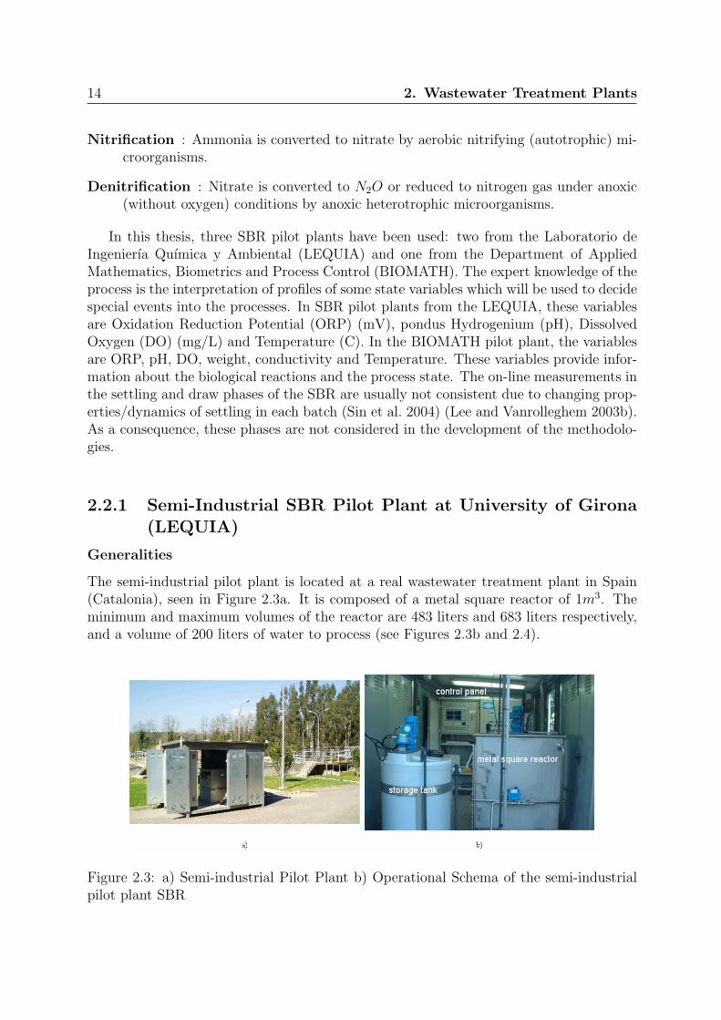


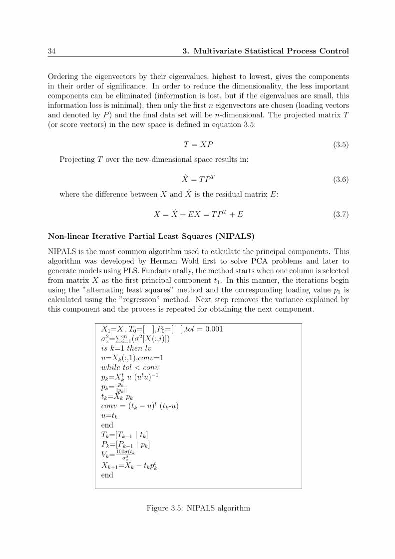


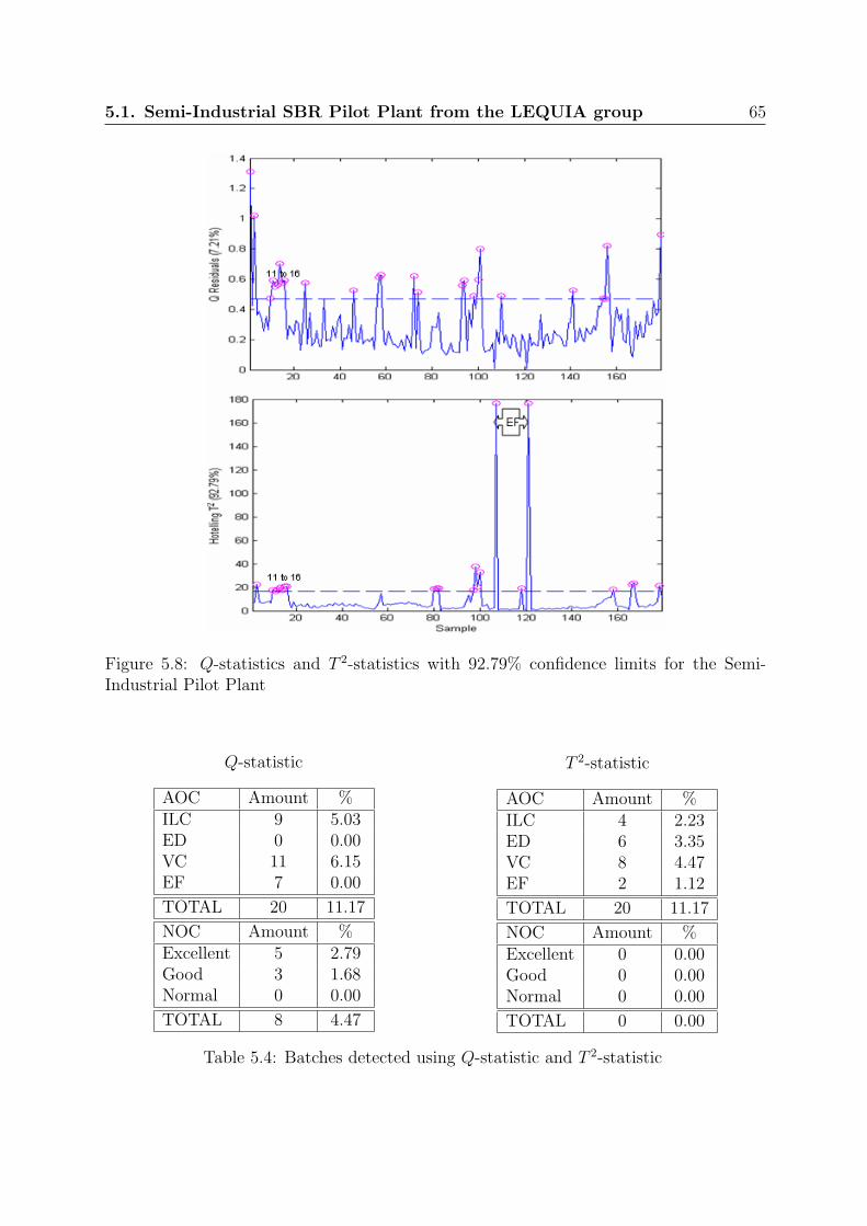


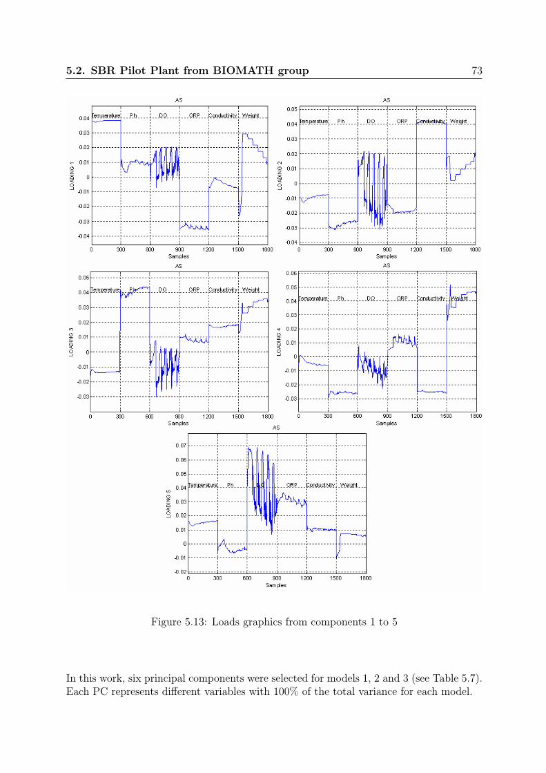


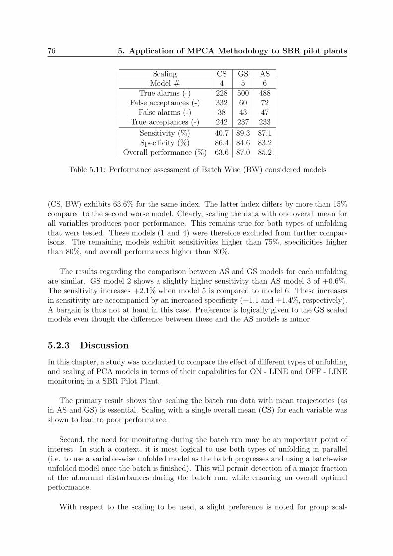


![Multivariate Statistical Analysis to Detect Insulin ... · Multivariate statistical analysis has been used as a process data history method that could help in such a situation [11].](https://static.documents.pub/doc/80x56/5e97c96cf2ac4e602d1a980e/multivariate-statistical-analysis-to-detect-insulin-multivariate-statistical.jpg)


