Multivariate Stochastic Volatility Models with Correlated Errors

By David Chan, Robert Kohn, Chris Kirby

WORKING PAPER(2006/04)

ISSN 13 29 12 70ISBN 0 7334 2335 3

CENTRE FOR APPLIEDECONOMIC RESEARCH

Multivariate Stochastic Volatility Models with

Correlated Errors

David Chana , Robert Kohnb∗, Chris Kirbyc

December 30, 2005

aMarketRx Inc, 1200 Route 22 East, Bridgewater NJ 08807 USAbFaculty of Commerce and Economics, School of Economics, John Goodsell Building

UNSW SYDNEY NSW 2052 AustraliacJohn E. Walker Department of Economics, Clemson University

222 Sirrine Hall, Clemson, SC 29634-1309 USA

Abstract

We develop a Bayesian approach for parsimoniously estimating the correlation structure

of the errors in a multivariate stochastic volatility model. Since the number of parameters

in the joint correlation matrix of the return and volatility errors is potentially very large,

we impose a prior that allows the off-diagonal elements of the inverse of the correlation

matrix to be identically zero. The model is estimated using a Markov chain simulation

method that samples from the posterior distribution of the volatilities and parameters.

We illustrate the approach using both simulated and real examples. In the real examples,

the method is applied to equities at three levels of aggregation: returns for firms within

the same industry, returns for different industries and returns aggregated at the index

level. We find pronounced correlation effects only at the highest level of aggregation.

Keywords: Bayesian estimation; Correlation matrix; Leverage; Markov chain Monte Carlo;

Model averaging.

JEL classification: C11, C15, C30

∗Corresponding author. EMAIL: R.Kohn@unsw.edu.au, TEL: +61 2 9385 2150

1

1 Introduction

A number of studies in financial economics report that conditional stock return volatility

responds asymmetrically to positive and negative return shocks. Well known examples

include French et al. (1987), Schwert (1990), Campbell and Hentschel (1992), Cheung

and Ng (1992), Engle and Ng (1993), Glosten et al. (1993), Braun et al. (1995), Bekaert

and Harvey (1997) and Bekaert and Wu (2000). Several explanations are proposed in

the literature for the existence of an asymmetric relation between volatility and returns.

The most widely cited of these is due to Black (1976) and Christie (1982) who suggest

that the asymmetry reflects changes in financial leverage. They argue in particular that

when a firm experiences a positive (negative) return, it becomes less (more) leveraged

due to the rise (fall) in the market value of its equity, thereby making it less (more) risky

and decreasing (increasing) its volatility. In other words, return shocks are negatively

correlated with volatility shocks.

Despite the long history of studying leverage effects in finance, econometricians are only

now beginning to allow for this type of asymmetry in stochastic volatility models because,

until recently, the latent nature of the volatility process made the estimation of such

models difficult using existing econometric methods. Often the only feasible strategy

was to either formulate a method of moments estimator, or develop a linear state-space

representation of the model and estimate it via quasi maximum likelihood (QML) using

the Kalman filter. Harvey and Shephard (1996) used the QML approach in one of the first

studies of leverage effects in a stochastic volatility framework. Over the last few years,

however, their approach has been supplanted by simulation-based methods for fitting

stochastic volatility models (see, e.g., Shephard and Pitt (1997), Durbin and Koopman

(1997), Kim et al. (1998), Sandmann and Koopman (1998), and Chib et al. (2002)). As

these methods gain wider recognition, more studies of models with leverage effects are

slowly making their way into the literature (e.g., Jacquier et al. (2004)).

Our article considers a multivariate stochastic volatility model that accommodates lever-

age effects by allowing a general correlation structure between the errors in the return

and volatility equations. Unlike univariate models, which are relatively straightforward

to handle, multivariate stochastic volatility models still pose significant computational

challenges to applied researchers because it is usually necessary to estimate a large num-

ber of parameters. One way to overcome this problem is to assume that the volatility

process for each asset has a factor structure, as in Chib et al. (2006), who successfully fit

a multivariate model with up to 50 stocks. However, the tractability of imposing a factor

model is not without cost because there is no guarantee that a factor structure with a

small number of factors is empirically plausible, and it may be difficult to interpret when

dealing with correlated errors.

The main contribution of this paper is to develop a general methodology for parsimo-

2

niously dealing with large dimensional correlation matrices in multivariate stochastic

volatility models. Although we consider one particular correlation structure in the ar-

ticle, our methods apply to other multivariate models, and in particular multivariate

factor models. Our methodology is Bayesian and uses ideas of Bayesian subset selection

and model averaging, which were first developed for the linear regression model, to achieve

a parsimonious representation of the joint correlation matrix of the errors for the return

and volatility equations. To see why we adopt this methodology, suppose we want to

fit a model involving 10 stocks. Under our model — a direct multivariate generalization

of the univariate log-linear specification — there are 190 unique parameters in the joint

correlation matrix of the errors. With this many free parameters, the estimation meth-

ods developed for the univariate case are not as effective and it is necessary to explicitly

control for the parameter-rich nature of the model in some way. Our approach imposes a

prior on the correlation matrix that allows the off-diagonal elements of the inverse of the

correlation matrix to be zero, which is equivalent to allowing the partial correlations of

the vector of returns and log volatilities to be zero.

This approach to parsimoniously estimating a covariance matrix is called covariance selec-

tion and is proposed by Wong et al. (2003). The basic idea of covariance selection is due

to Dempster (1972), who suggests zeroing out elements of the inverse of the covariance

matrix (based on the data) to obtain a parsimonious, and hence more efficient, estimate

of the covariance matrix. The approach by Wong et al. (2003) is adapted by Pitt et al.

(2005) to estimate a correlation matrix. In our case, the time varying covariance matrix

is factored into a product of variances and a correlation matrix, with the log variances

following independent stochastic volatility processes. Such a decomposition of variances

and a correlation matrix is similar to the decomposition in Barnard et al. (2000), but they

do not allow elements of the correlation matrix or its inverse to be zero and the variances

do not have a time series structure. The computations are carried out using a Markov

chain Monte Carlo simulation method.

We illustrate the methodology using both simulated and real data. The simulation results

show that our methodology works well and recovers the correct degree of parsimony both

when the cross-correlation between the return errors and the volatility errors is zero and

when it is present. We also fit the model to real daily stock returns for the period January

1988 to December 2001, which we analyze at three different levels of aggregation. First, we

use the returns on several sets of individual stocks that are grouped according to industry.

Second, we use the returns on a set of narrowly-defined portfolios constructed by giving

equal weights to the firms within the industry groups. Finally, we use the returns on a

set of broadly-based portfolios that correspond to different market indexes. This covers

all the three types of return data that are used in the finance literature to investigate

leverage effects.

The paper is organized as follows. Section 2 introduces the stochastic volatility model and

its multivariate extension, discusses the prior assumptions and the Markov chain Monte

3

Carlo sampling scheme. Section 3 presents some empirical results from applying our

method to simulated data and section 4 presents the results from applying our method

to equity returns data aggregated at three different levels. We conclude with a short

discussion in section 5. An appendix gives details of the sampling scheme.

2 Model, prior and sampling scheme

2.1 Model description

To simplify the exposition, we assume a zero mean for the returns process throughout

this paper. The basic univariate stochastic volatility model in our article is

yt = exp (ht/2) et, (2.1)

ht = µ+ φ(ht−1 − µ) + ψat, (2.2)

where yt is the return at time t and exp(ht/2) is the volatility at time t. We assume

that the log variance ht follows a first order autoregressive process with mean µ and

persistence parameter φ. We also assume that (et, at)′ is bivariate normal with zero

mean, var(et) = var(at) = 1, and with ρ the correlation between et and at. Jacquier et al.

(2004) estimate a similar model, but also allow for fat-tailed errors. These authors note

that when the correlation ρ < 0, positive and negative shocks et have asymmetric effects

on volatility. Specifically, if et is negative, then at is likely to be positive with a consequent

increase in volatility, whereas a positive et is likely to result in a negative value of at and

hence a decrease in volatility. Chib et al. (2002) estimate such a model with ρ = 0, but

allow for jumps and fat-tailed errors.

We use the following generalization of the univariate model (2.1) and (2.2) due to Harvey,

Ruiz and Shephard (1994) and Danielsson (1998). Let yt = (yt1, . . . , ytp)′ be the p × 1

vector of returns at time t and ht be the corresponding vector of log variances, such that

yt = S12

t et, (2.3)

ht = µ+ Φ(ht−1 − µ) + Ψ12at, (2.4)

where St = diag(exp(ht1), . . . , exp(htp)), µ = (µ1, . . . , µp)′, and Φ and Ψ are diagonal

matrices whose diagonals are the vectors φ = (φ1, . . . , φp)′ and ψ = (ψ2

1, . . . , ψ2p)

′. Let

rt = (e′t, a′t)

′. We assume that rt is multivariate normal with zero mean, and covariance

matrix C, with C a correlation matrix, that is, it has ones on the diagonal. This means

that et ∼ N(0, C1) and at ∼ N(0, C2), where C1 is the p×p upper left submatrix of C and

C2 is the p× p lower right submatrix of C. Let C12 = cov(et, at), which is the covariance

matrix of the errors in the observation and volatility equations.

A number of authors investigate the following modification of the univariate stochastic

volatility model, for example Harvey and Shephard (1996), Meyer and Yu (2000) and Yu

4

(2005); (2.1) stays the same, but the volatility evolution equation (2.2) is

ht+1 = µ+ φ(ht − µ) + ψat, (2.5)

which means that a shock to et affects ht+1 rather than ht. Yu (2005) argues that this

modification is appealing from a theoretical perspective because it implies that yt is a

martingale difference sequence. In the multivariate version of the model the observation

equation is still (2.4), but the volatility evolution equation is

ht+1 = µ+ Φ(ht − µ) + Ψ12at . (2.6)

Although we do not fit this model as part of the empirical analysis, it is straightforward

to adapt the covariance selection approach proposed in our article to this model.

An alternative approach to estimating a multivariate stochastic volatility model is to

impose a factor structure. The simplest specification of the factor model is

yt = BF t + Σ12 et, et ∼ MVNp(0, I) , (2.7)

Ft ∼ MVNk(0, St) , (2.8)

ht = µ+ Φ(ht−1 − µ) + Ψ12at, at ∼ MVNk(0, I) , (2.9)

where Ft = (Ft1, . . . , Ftk)′ are k underlying time varying factors with zero mean and co-

variance matrix St = diag(exp(ht1), . . . , exp(htk)) and B = (B1, . . . , Bk) is a p×k matrix

of factor loadings. The log variances, hti, i = 1, . . . , k are assumed to be independent and

Σ = diag(σ21, . . . , σ

2p) is a constant matrix, giving a time-varying covariance matrix for

the process as BStB′ + Σ. The number of factors used is typically small compared to the

number of series considered. See Pitt and Shephard (1999), Jacquier et al. (1999), Chib

et al. (2006). However, these authors do not consider correlated errors.

We could incorporate correlated errors into the model (2.7) – (2.9) by allowing et and at to

be correlated, but it would be difficult to interpret these correlations in terms of individual

returns and volatilities because there are now two sources of volatility, from the et and

also from the factors. Thus our approach may be preferred to the factor approach in many

applications. We note that although the factor model allows for changing correlations,

it assumes that the matrix of factor loadings is constant. It does not necessarily follow,

therefore, that a factor model with time-varying correlations will outperform a non-factor

model that assumes constant correlations. This is an empirical question that we do not

attempt to answer in this article.

The development of new multivariate models continues to be an active area of research.

Asai and McAleer (2005) propose a dynamic asymmetric leverage (DAL) model that ac-

commodates threshold effects, i.e., it allows volatility to undergo discrete shifts depending

on whether the return for the previous period is above or below some threshold value.

This type of specification offers a potential avenue for extending our covariance selec-

tion methodology. Additional examples of multivariate stochastic volatility models are

5

provided in McAleer (2005), Asai and McAleer (2006), and Yu and Meyer (2006). To sim-

plify the discussion we henceforth refer to any model that allows for correlation between

the errors in the observation equation and volatility transition equation as a stochastic

volatility model with leverage. Model selection criteria plus subject matter knowledge

can be used to select which of the alternative models is best for any particular data set.

2.2 Prior specification

The joint prior specification for Θ = (µ, φ, ψ, C) assumes that they are independent of

each other and that the elements of φ and ψ are independent of each other. That is

p(µ, φ, ψ, C) = p(µ)p(C)

(p∏

i=1

p(φi)

)(p∏

i=1

p(ψ2i )

).

The prior on φi, i = 1, . . . , p, is uniform on (−1, 1), which ensures the stationarity of the

volatility process. The prior on µ is taken proportional to a constant, which is the usual

noninformative prior on log variances. The prior on ψ2i is assumed to be inverse gamma

with parameters (α, β),

(ψ2i )

−(1+α) exp(−β/ψ2i )β

α

Γ(α).

We set α = 10e−10 and β = 10e−3, making the prior uninformative. In our work it is

more convenient to work with vi = (ψ2i )

− 12 , i = 1, . . . , p, and generate V = (v1, . . . , vp)

′

as a block. The prior for V is

p(V ) ∝

p∏

i=1

v2α−1i exp(−βV ′V ) .

The elements of the correlation matrix C are not generated directly but are parameterized

in terms of a matrix D, where C−1 = TDT with D a correlation matrix and T a diagonal

matrix, such that

Ti = (D−1)12

ii , i = 1, . . . , 2p,

because C is a correlation matrix. We perform element selection on the off-diagonal

elements of the matrix D, allowing them to be set to zero explicitly. The prior for

D is proposed by Wong et al. (2003) and the important details are repeated here for

completeness.

To describe the prior, let Jij = 1 if Dij 6≡ 0 and Jij = 0 if Dij ≡ 0, for i = 1, . . . , 2p, j < i.

That is, Jij is a binary variable that indicates whether the element Dij in the strict lower

triangle of D is identically zero or not. Let J = Jij, i = 1, . . . , 2p, j < i, i.e., the

6

ensemble of all the Jij and let J\ij be J with Jij excluded. Let S(J) be the number of

elements in J that are 1, and let S(J\ij) be the number of elements in J\ij that are 1.

Let DJ=1 = Dij : Jij ∈ J and Jij = 1 and DJ=0 = Dij : Jij ∈ J and Jij = 0. Let

C2p be the class of all 2p× 2p correlation matrices. Let

V (J) =

∫

D∈C2p

dDJ=1

be the volume of the correlation matrix for given configuration J , let m = 2p(2p− 1)/2,

and let

V (l) =

(m

l

)−1 ∑

J :S(J)=l

V (J)

be the average volume of all matrices having exactly l nonzero elements. Wong et al.

(2003) propose the following hierarchical prior for D.

p(dD | J) = V (J)−1dDJ=1I(D ∈ C2p) ,

p(J | S(J) = l) =V (J)

V (l)

(m

l

)−1

, (2.10)

p(S(J) = l | ϕ) =

(m

l

)ϕl(1 − ϕ)m−l ,

where 0 ≤ ϕ ≤ 1 and is interpreted as the probability that Jij = 1. Thus p(D | J) is

uniform, the prior for J given S(J) = l is uniform up to a volume adjustment, and the

prior for S(J), given ϕ, is binomial. Wong et al. (2003) assume that ϕ is uniform on (0, 1)

and show that with this prior,

p(S = l) =1

m+ 1,

i.e., S is uniformly distributed in model size.

To simplify the computations, we approximate (2.10) by

p(J | S(J) = l) =

(m

l

)−1

in our applications. This simplification has a minor effect on the empirical results for the

size of correlation matrices used in the article.

2.3 Markov chain Monte Carlo sampling scheme

The MCMC sampling scheme used to estimate the parameters of the multivariate model

is now outlined, with the technical details given in the appendix. Let y = (y1, . . . , yn)′

and h = (h1, . . . , hn)′. Step 0 is an initialization step and the sampling scheme cycles

through the following 5 steps using 1000 iterations for burn-in and 10000 iterations for

inference.

7

0. Initialize Θ and h.

The parameters Θ and the volatility h are initialized by fitting univariate stochastic

volatility models to each series. Given the other parameters, C is initialized to the

estimate of the correlation matrix of the rt, where rt is defined in section 2.1.

1. φ | y, h, C, µ, ψ

The vector φ is generated using the Metropolis-Hastings method with a multivariate

Gaussian proposal density such that each φi constrained to lie between −1 and 1.

2. µ | y, h, C, φ, ψ

The conditional distribution of µ is multivariate Gaussian.

3. V | y, h, C, φ, µ

The conditional distribution of V is not standard, so V is generated using the

Metropolis-Hastings method with a proposal density that is multivariate-t, and

centered around the mode of the conditional density.

4. h | y,Θ

The Markovian structure of the model can be exploited to simplify the posterior of

h to a series of univariate conditional densities,

p(ht | ht−1, ht+1, yt−1, yt+1, C, φ, µ, ψ), t = 1, . . . , n .

The ht can be generated one at a time, but experimentation shows that this strategy

converges slowly and mixes poorly. Instead, h is generated in blocks as in Shephard

and Pitt (1997). Let ha:b = (ha, ha+1, . . . , hb) denote the block of log variances

that we wish to generate and h\a:b denote all of h excluding ha:b. The block size

is randomly chosen to be 1, 2 or 3 with equal probability at each stage. The

conditional distribution of the block, p(ha:b | h\a:b, y,Θ), is not tractable and the

Metropolis-Hastings method is used with a Gaussian proposal density.

5. C | y, h, φ, µ, ψ

The parsimonious correlation matrix estimation method of Wong et al. (2003), as

modified by Pitt et al. (2005), is used to estimate C. The details are in the appendix.

2.4 Inference

Inference on the parameters follows the standard Bayesian approach of looking at func-

tionals of the posterior distributions. For example, the posterior mean estimate of the log

variance is given by

ht =1

L

L∑

l=1

h[l]t i = 1, . . . , p, t = 1, . . . , n .

8

where h[l]t is the lth iterate from the inference stage. Similarly, the posterior mean estimate

of ψi is

ψi =1

L

L∑

l=1

(v

[l]i

)−2

i = 1, . . . , p ,

and the posterior mean estimate of φi is

φi =1

L

L∑

l=1

φ[l]i i = 1, . . . , p .

where v[l]i and φ

[l]i are the lth iterate from the inference stage.

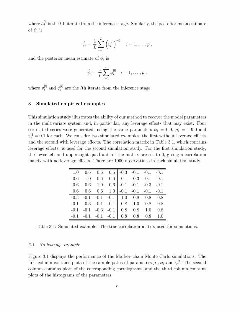
3 Simulated empirical examples

This simulation study illustrates the ability of our method to recover the model parameters

in the multivariate system and, in particular, any leverage effects that may exist. Four

correlated series were generated, using the same parameters φi = 0.9, µi = −9.0 and

ψ2i = 0.1 for each. We consider two simulated examples, the first without leverage effects

and the second with leverage effects. The correlation matrix in Table 3.1, which contains

leverage effects, is used for the second simulation study. For the first simulation study,

the lower left and upper right quadrants of the matrix are set to 0, giving a correlation

matrix with no leverage effects. There are 1000 observations in each simulation study.

1.0 0.6 0.6 0.6 -0.3 -0.1 -0.1 -0.1

0.6 1.0 0.6 0.6 -0.1 -0.3 -0.1 -0.1

0.6 0.6 1.0 0.6 -0.1 -0.1 -0.3 -0.1

0.6 0.6 0.6 1.0 -0.1 -0.1 -0.1 -0.1

-0.3 -0.1 -0.1 -0.1 1.0 0.8 0.8 0.8

-0.1 -0.3 -0.1 -0.1 0.8 1.0 0.8 0.8

-0.1 -0.1 -0.3 -0.1 0.8 0.8 1.0 0.8

-0.1 -0.1 -0.1 -0.1 0.8 0.8 0.8 1.0

Table 3.1: Simulated example: The true correlation matrix used for simulations.

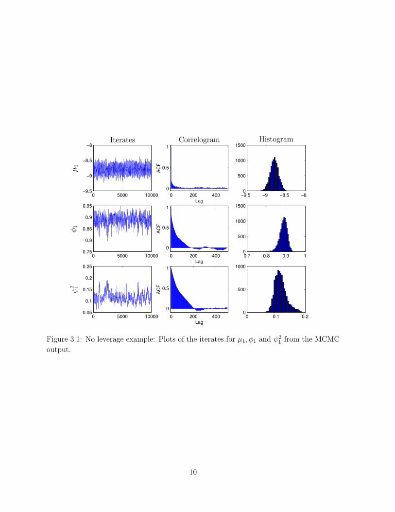
3.1 No leverage example

Figure 3.1 displays the performance of the Markov chain Monte Carlo simulations. The

first column contains plots of the sample paths of parameters µ1, φ1 and ψ21. The second

column contains plots of the corresponding correlograms, and the third column contains

plots of the histograms of the parameters.

9

0 5000 10000−9.5

−9

−8.5

−8

0 200 4000

0.5

1

Lag

AC

F

−9.5 −9 −8.5 −80

500

1000

1500

0 5000 100000.75

0.8

0.85

0.9

0.95

0.7 0.8 0.9 10

500

1000

1500

0 5000 100000.05

0.1

0.15

0.2

0.25

0 200 400

0

0.5

1

Lag

AC

F

0 0.1 0.20

500

1000

0 200 400

0

0.5

1

Lag

AC

F

PSfrag replacements

µ1

φ1

ψ2 1

Iterates Correlogram Histogram

Figure 3.1: No leverage example: Plots of the iterates for µ1, φ1 and ψ21 from the MCMC

output.

10

0 100 200 300 400 500 600 700 800 900 1000−12

−10

−8

−6

0 100 200 300 400 500 600 700 800 900 1000−12

−10

−8

−6

0 100 200 300 400 500 600 700 800 900 1000−12

−10

−8

−6

0 100 200 300 400 500 600 700 800 900 1000−12

−10

−8

−6

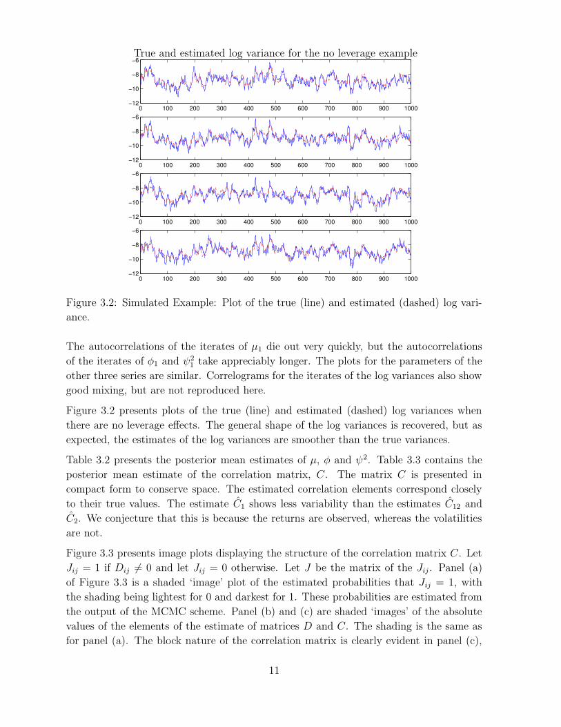
PSfrag replacements

True and estimated log variance for the no leverage example

Figure 3.2: Simulated Example: Plot of the true (line) and estimated (dashed) log vari-

ance.

The autocorrelations of the iterates of µ1 die out very quickly, but the autocorrelations

of the iterates of φ1 and ψ21 take appreciably longer. The plots for the parameters of the

other three series are similar. Correlograms for the iterates of the log variances also show

good mixing, but are not reproduced here.

Figure 3.2 presents plots of the true (line) and estimated (dashed) log variances when

there are no leverage effects. The general shape of the log variances is recovered, but as

expected, the estimates of the log variances are smoother than the true variances.

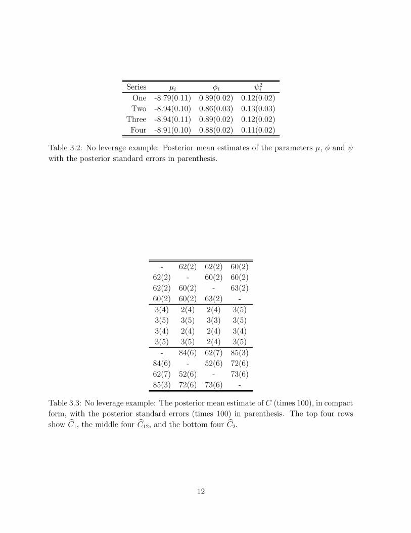
Table 3.2 presents the posterior mean estimates of µ, φ and ψ2. Table 3.3 contains the

posterior mean estimate of the correlation matrix, C. The matrix C is presented in

compact form to conserve space. The estimated correlation elements correspond closely

to their true values. The estimate C1 shows less variability than the estimates C12 and

C2. We conjecture that this is because the returns are observed, whereas the volatilities

are not.

Figure 3.3 presents image plots displaying the structure of the correlation matrix C. Let

Jij = 1 if Dij 6= 0 and let Jij = 0 otherwise. Let J be the matrix of the Jij. Panel (a)

of Figure 3.3 is a shaded ‘image’ plot of the estimated probabilities that Jij = 1, with

the shading being lightest for 0 and darkest for 1. These probabilities are estimated from

the output of the MCMC scheme. Panel (b) and (c) are shaded ‘images’ of the absolute

values of the elements of the estimate of matrices D and C. The shading is the same as

for panel (a). The block nature of the correlation matrix is clearly evident in panel (c),

11

Series µi φi ψ2i

One -8.79(0.11) 0.89(0.02) 0.12(0.02)

Two -8.94(0.10) 0.86(0.03) 0.13(0.03)

Three -8.94(0.11) 0.89(0.02) 0.12(0.02)

Four -8.91(0.10) 0.88(0.02) 0.11(0.02)

Table 3.2: No leverage example: Posterior mean estimates of the parameters µ, φ and ψ

with the posterior standard errors in parenthesis.

- 62(2) 62(2) 60(2)

62(2) - 60(2) 60(2)

62(2) 60(2) - 63(2)

60(2) 60(2) 63(2) -

3(4) 2(4) 2(4) 3(5)

3(5) 3(5) 3(3) 3(5)

3(4) 2(4) 2(4) 3(4)

3(5) 3(5) 2(4) 3(5)

- 84(6) 62(7) 85(3)

84(6) - 52(6) 72(6)

62(7) 52(6) - 73(6)

85(3) 72(6) 73(6) -

Table 3.3: No leverage example: The posterior mean estimate of C (times 100), in compact

form, with the posterior standard errors (times 100) in parenthesis. The top four rows

show C1, the middle four C12, and the bottom four C2.

12

1 2 3 4 5 6 7 8

1

2

3

4

5

6

7

8

PSfrag replacements

(a) - J

(b) - D

(c) - C1 2 3 4 5 6 7 8

1

2

3

4

5

6

7

8

PSfrag replacements

(a) - J

(b) - D

(c) - C1 2 3 4 5 6 7 8

1

2

3

4

5

6

7

8

PSfrag replacements

(a) - J

(b) - D

(c) - C

Figure 3.3: No leverage example: (a) Shaded ‘image’ of the estimated probability of

Jij = 1. Panels (b) and (c) are shaded ‘images’ of the absolute values of the elements of

the posterior mean estimate of matrices D and C.

highlighting the ability of our methodology to pick up parsimony where it exists.

3.2 Leverage example

This section summarizes the results for the second simulated example, when leverage

effects are present. Tables 3.4 and 3.5 present the posterior mean estimates of the para-

meters µ, φ, ψ and C. The parameter estimates for µ, φ and ψ are quite similar for both

examples, but leverage effects are now identified in the estimate of the correlation matrix

C, as well as in the image plots in Figure 3.4.

Series µi φi ψ2i

One -8.82(0.10) 0.89(0.02) 0.12(0.02)

Two -8.90(0.09) 0.86(0.03) 0.12(0.03)

Three -8.91(0.11) 0.89(0.02) 0.12(0.02)

Four -8.90(0.10) 0.88(0.02) 0.11(0.02)

Table 3.4: Leverage example: Posterior mean estimates of the parameters µ, φ and ψ

with the posterior standard errors in parenthesis.

The acceptance rates for the sampling of h are high for both examples. For the example

with no leverage, the acceptance rate is 99.2% for a block size of one, 98.0% for a block

size of 2 and 96.5% for a block size of 3. We obtain similarly high acceptance rates for

the leverage example.

4 Equity returns example

We now apply our methods to equity returns data aggregated at 3 different levels. The first

level is the market index level. There are eight return series in the following order: return

13

- 62(2) 62(2) 61(2)

62(2) - 60(2) 60(2)

62(2) 60(2) - 64(2)

61(2) 60(2) 64(2) -

-19(7) -5(8) -5(8) -9(8)

1(8) -22 (7) -5(7) 4(8)

-4(7) -1(8) -26(7) -1(10)

6(8) -1(8) -14(8) -21(7)

- 73(6) 66(7) 74(5)

73(6) - 54(8) 62(7)

66(7) 54(8) - 61(8)

74(5) 62(7) 61(8) -

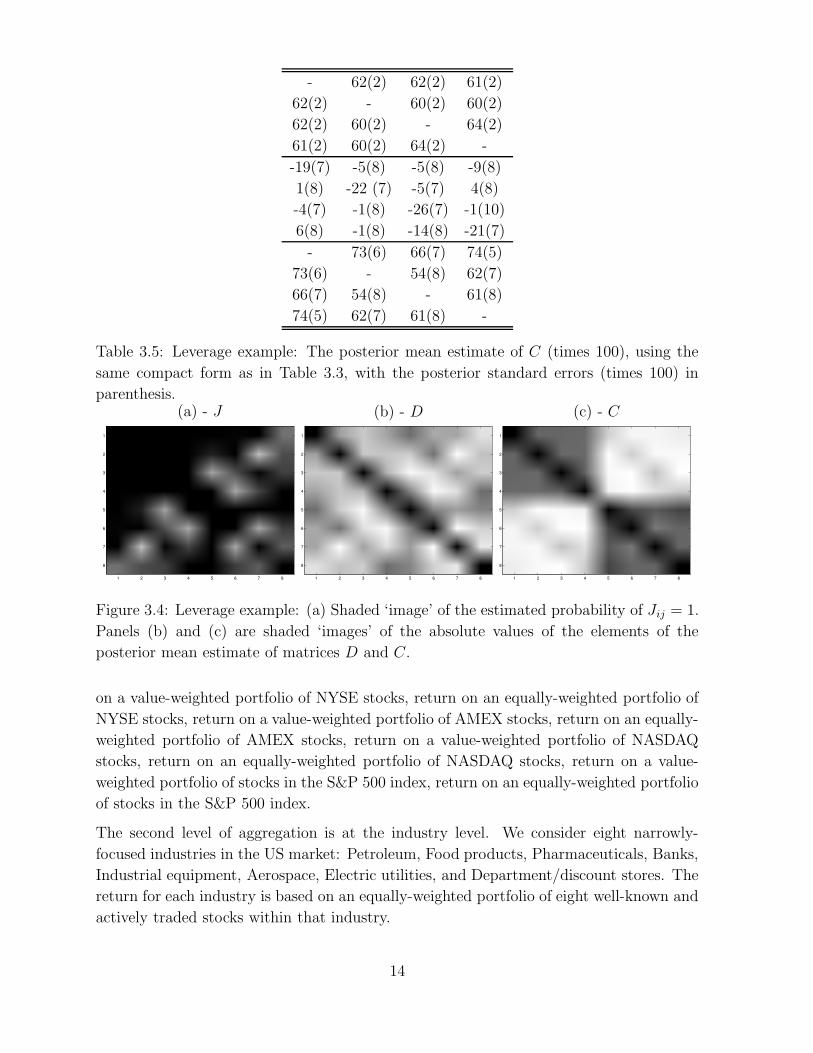
Table 3.5: Leverage example: The posterior mean estimate of C (times 100), using the

same compact form as in Table 3.3, with the posterior standard errors (times 100) in

parenthesis.

1 2 3 4 5 6 7 8

1

2

3

4

5

6

7

8

PSfrag replacements

(a) - J

(b) - D

(c) - C1 2 3 4 5 6 7 8

1

2

3

4

5

6

7

8

PSfrag replacements

(a) - J

(b) - D

(c) - C1 2 3 4 5 6 7 8

1

2

3

4

5

6

7

8

PSfrag replacements

(a) - J

(b) - D

(c) - C

Figure 3.4: Leverage example: (a) Shaded ‘image’ of the estimated probability of Jij = 1.

Panels (b) and (c) are shaded ‘images’ of the absolute values of the elements of the

posterior mean estimate of matrices D and C.

on a value-weighted portfolio of NYSE stocks, return on an equally-weighted portfolio of

NYSE stocks, return on a value-weighted portfolio of AMEX stocks, return on an equally-

weighted portfolio of AMEX stocks, return on a value-weighted portfolio of NASDAQ

stocks, return on an equally-weighted portfolio of NASDAQ stocks, return on a value-

weighted portfolio of stocks in the S&P 500 index, return on an equally-weighted portfolio

of stocks in the S&P 500 index.

The second level of aggregation is at the industry level. We consider eight narrowly-

focused industries in the US market: Petroleum, Food products, Pharmaceuticals, Banks,

Industrial equipment, Aerospace, Electric utilities, and Department/discount stores. The

return for each industry is based on an equally-weighted portfolio of eight well-known and

actively traded stocks within that industry.

14

The third level of aggregation is at the individual firm level. For each of the industries

specified above, we consider the return on each firm within that industry. The sample

period for all the equity data is from January 4, 1988 to December 29, 2001, giving a total

of 3285 observations. All the data is mean corrected so the returns have zero means.

4.1 Individual firms return data

For conciseness, we show only the results for the eight firms in the Petroleum industry.

The results for the firms in the other seven industries are similar.

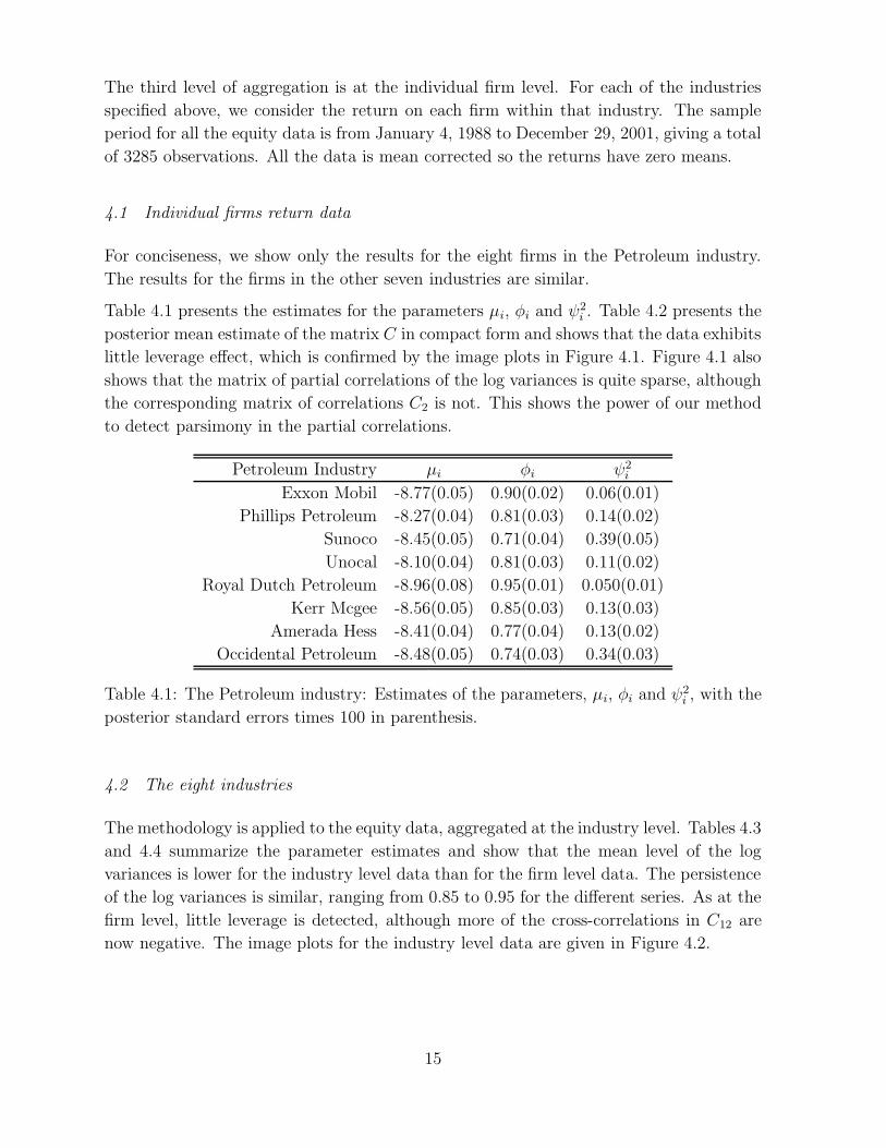
Table 4.1 presents the estimates for the parameters µi, φi and ψ2i . Table 4.2 presents the

posterior mean estimate of the matrix C in compact form and shows that the data exhibits

little leverage effect, which is confirmed by the image plots in Figure 4.1. Figure 4.1 also

shows that the matrix of partial correlations of the log variances is quite sparse, although

the corresponding matrix of correlations C2 is not. This shows the power of our method

to detect parsimony in the partial correlations.

Petroleum Industry µi φi ψ2i

Exxon Mobil -8.77(0.05) 0.90(0.02) 0.06(0.01)

Phillips Petroleum -8.27(0.04) 0.81(0.03) 0.14(0.02)

Sunoco -8.45(0.05) 0.71(0.04) 0.39(0.05)

Unocal -8.10(0.04) 0.81(0.03) 0.11(0.02)

Royal Dutch Petroleum -8.96(0.08) 0.95(0.01) 0.050(0.01)

Kerr Mcgee -8.56(0.05) 0.85(0.03) 0.13(0.03)

Amerada Hess -8.41(0.04) 0.77(0.04) 0.13(0.02)

Occidental Petroleum -8.48(0.05) 0.74(0.03) 0.34(0.03)

Table 4.1: The Petroleum industry: Estimates of the parameters, µi, φi and ψ2i , with the

posterior standard errors times 100 in parenthesis.

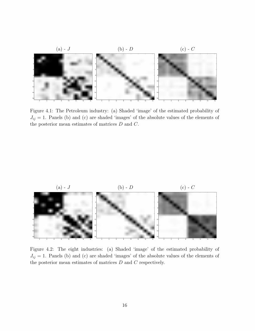
4.2 The eight industries

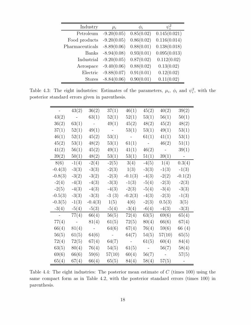
The methodology is applied to the equity data, aggregated at the industry level. Tables 4.3

and 4.4 summarize the parameter estimates and show that the mean level of the log

variances is lower for the industry level data than for the firm level data. The persistence

of the log variances is similar, ranging from 0.85 to 0.95 for the different series. As at the

firm level, little leverage is detected, although more of the cross-correlations in C12 are

now negative. The image plots for the industry level data are given in Figure 4.2.

15

2 4 6 8 10 12 14 16

2

4

6

8

10

12

14

16

PSfrag replacements

(a) - J

(b) - D

(c) - C2 4 6 8 10 12 14 16

2

4

6

8

10

12

14

16

PSfrag replacements

(a) - J

(b) - D

(c) - C2 4 6 8 10 12 14 16

2

4

6

8

10

12

14

16

PSfrag replacements

(a) - J

(b) - D

(c) - C

Figure 4.1: The Petroleum industry: (a) Shaded ‘image’ of the estimated probability of

Jij = 1. Panels (b) and (c) are shaded ‘images’ of the absolute values of the elements of

the posterior mean estimates of matrices D and C.

2 4 6 8 10 12 14 16

2

4

6

8

10

12

14

16

PSfrag replacements

(a) - J

(b) - D

(c) - C2 4 6 8 10 12 14 16

2

4

6

8

10

12

14

16

PSfrag replacements

(a) - J

(b) - D

(c) - C2 4 6 8 10 12 14 16

2

4

6

8

10

12

14

16

PSfrag replacements

(a) - J

(b) - D

(c) - C

Figure 4.2: The eight industries: (a) Shaded ‘image’ of the estimated probability of

Jij = 1. Panels (b) and (c) are shaded ‘images’ of the absolute values of the elements of

the posterior mean estimates of matrices D and C respectively.

16

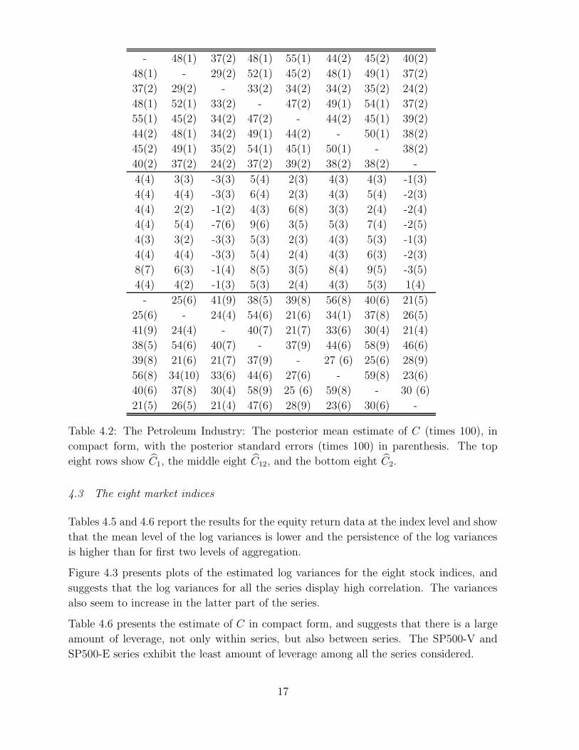
- 48(1) 37(2) 48(1) 55(1) 44(2) 45(2) 40(2)

48(1) - 29(2) 52(1) 45(2) 48(1) 49(1) 37(2)

37(2) 29(2) - 33(2) 34(2) 34(2) 35(2) 24(2)

48(1) 52(1) 33(2) - 47(2) 49(1) 54(1) 37(2)

55(1) 45(2) 34(2) 47(2) - 44(2) 45(1) 39(2)

44(2) 48(1) 34(2) 49(1) 44(2) - 50(1) 38(2)

45(2) 49(1) 35(2) 54(1) 45(1) 50(1) - 38(2)

40(2) 37(2) 24(2) 37(2) 39(2) 38(2) 38(2) -

4(4) 3(3) -3(3) 5(4) 2(3) 4(3) 4(3) -1(3)

4(4) 4(4) -3(3) 6(4) 2(3) 4(3) 5(4) -2(3)

4(4) 2(2) -1(2) 4(3) 6(8) 3(3) 2(4) -2(4)

4(4) 5(4) -7(6) 9(6) 3(5) 5(3) 7(4) -2(5)

4(3) 3(2) -3(3) 5(3) 2(3) 4(3) 5(3) -1(3)

4(4) 4(4) -3(3) 5(4) 2(4) 4(3) 6(3) -2(3)

8(7) 6(3) -1(4) 8(5) 3(5) 8(4) 9(5) -3(5)

4(4) 4(2) -1(3) 5(3) 2(4) 4(3) 5(3) 1(4)

- 25(6) 41(9) 38(5) 39(8) 56(8) 40(6) 21(5)

25(6) - 24(4) 54(6) 21(6) 34(1) 37(8) 26(5)

41(9) 24(4) - 40(7) 21(7) 33(6) 30(4) 21(4)

38(5) 54(6) 40(7) - 37(9) 44(6) 58(9) 46(6)

39(8) 21(6) 21(7) 37(9) - 27 (6) 25(6) 28(9)

56(8) 34(10) 33(6) 44(6) 27(6) - 59(8) 23(6)

40(6) 37(8) 30(4) 58(9) 25 (6) 59(8) - 30 (6)

21(5) 26(5) 21(4) 47(6) 28(9) 23(6) 30(6) -

Table 4.2: The Petroleum Industry: The posterior mean estimate of C (times 100), in

compact form, with the posterior standard errors (times 100) in parenthesis. The top

eight rows show C1, the middle eight C12, and the bottom eight C2.

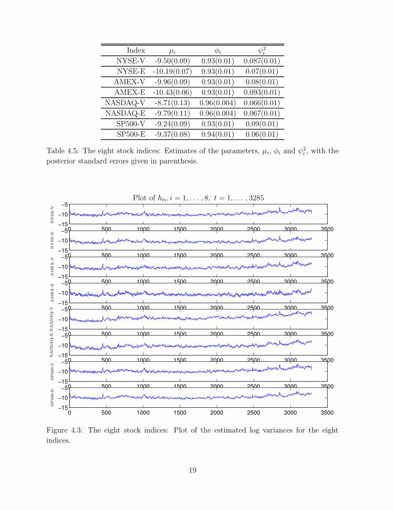
4.3 The eight market indices

Tables 4.5 and 4.6 report the results for the equity return data at the index level and show

that the mean level of the log variances is lower and the persistence of the log variances

is higher than for first two levels of aggregation.

Figure 4.3 presents plots of the estimated log variances for the eight stock indices, and

suggests that the log variances for all the series display high correlation. The variances

also seem to increase in the latter part of the series.

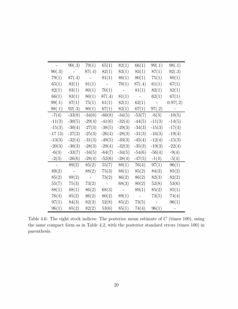
Table 4.6 presents the estimate of C in compact form, and suggests that there is a large

amount of leverage, not only within series, but also between series. The SP500-V and

SP500-E series exhibit the least amount of leverage among all the series considered.

17

Industry µi φi ψ2i

Petroleum -9.20(0.05) 0.85(0.02) 0.145(0.021)

Food products -9.20(0.05) 0.86(0.02) 0.116(0.014)

Pharmaceuticals -8.89(0.06) 0.88(0.01) 0.138(0.018)

Banks -8.94(0.08) 0.93(0.01) 0.095(0.013)

Industrial -9.20(0.05) 0.87(0.02) 0.112(0.02)

Aerospace -9.40(0.06) 0.88(0.02) 0.13(0.02)

Electric -9.88(0.07) 0.91(0.01) 0.12(0.02)

Stores -8.84(0.06) 0.90(0.01) 0.11(0.02)

Table 4.3: The eight industries: Estimates of the parameters, µi, φi and ψ2i , with the

posterior standard errors given in parenthesis.

- 43(2) 36(2) 37(1) 46(1) 45(2) 40(2) 39(2)

43(2) - 63(1) 52(1) 52(1) 53(1) 56(1) 50(1)

36(2) 63(1) - 49(1) 45(2) 48(2) 45(2) 48(2)

37(1) 52(1) 49(1) - 53(1) 53(1) 49(1) 53(1)

46(1) 52(1) 45(2) 53(1) - 61(1) 41(1) 53(1)

45(2) 53(1) 48(2) 53(1) 61(1) - 46(2) 51(1)

41(2) 56(1) 45(2) 49(1) 41(1) 46(2) - 39(1)

39(2) 50(1) 48(2) 53(1) 53(1) 51(1) 39(1) -

8(6) -1(4) -2(4) -2(5) 3(4) -4(5) 1(4) 0.3(4)

-0.4(3) -3(3) -3(3) -2(3) 1(3) -3(3) -1(3) -1(3)

-0.8(3) -3(2) -3(2) -2(3) -0.1(3) -4(3) -2(2) -0.1(2)

-2(4) -4(3) -4(3) -3(3) -1(3) -5(4) -2(3) -2(3)

-2(5) -4(3) -4(3) -4(3) -2(3) -5(4) -3(4) -3(3)

-0.5(3) -3(3) -3(3) -3 (3) -0.2(3) -4(3) -2(3) -1(3)

-0.3(5) -1(3) -0.4(3) 1(5) 4(6) -2(3) 0.5(3) 3(5)

-3(4) -5(4) -5(3) -5(4) -3(4) -6(4) -4(3) -3(3)

- 77(4) 66(4) 56(5) 72(4) 63(5) 69(6) 65(4)

77(4) - 81(4) 61(5) 72(5) 80(4) 66(6) 67(4)

66(4) 81(4) - 64(6) 67(4) 76(4) 59(6) 66 (4)

56(5) 61(5) 64(6) - 64(7) 54(5) 57(10) 65(5)

72(4) 72(5) 67(4) 64(7) - 61(5) 60(4) 84(4)

63(5) 80(4) 76(4) 54(5) 61(5) - 56(7) 58(4)

69(6) 66(6) 59(6) 57(10) 60(4) 56(7) - 57(5)

65(4) 67(4) 66(4) 65(5) 84(4) 58(4) 57(5) -

Table 4.4: The eight industries: The posterior mean estimate of C (times 100) using the

same compact form as in Table 4.2, with the posterior standard errors (times 100) in

parenthesis.

18

Index µi φi ψ2i

NYSE-V -9.50(0.09) 0.93(0.01) 0.087(0.01)

NYSE-E -10.19(0.07) 0.93(0.01) 0.07(0.01)

AMEX-V -9.96(0.09) 0.93(0.01) 0.08(0.01)

AMEX-E -10.43(0.06) 0.93(0.01) 0.093(0.01)

NASDAQ-V -8.71(0.13) 0.96(0.004) 0.066(0.01)

NASDAQ-E -9.79(0.11) 0.96(0.004) 0.067(0.01)

SP500-V -9.24(0.09) 0.93(0.01) 0.09(0.01)

SP500-E -9.37(0.08) 0.94(0.01) 0.06(0.01)

Table 4.5: The eight stock indices: Estimates of the parameters, µi, φi and ψ2i , with the

posterior standard errors given in parenthesis.

0 500 1000 1500 2000 2500 3000 3500−15

−10

−5

0 500 1000 1500 2000 2500 3000 3500−15

−10

−5

0 500 1000 1500 2000 2500 3000 3500−15

−10

−5

0 500 1000 1500 2000 2500 3000 3500−15

−10

−5

0 500 1000 1500 2000 2500 3000 3500−15

−10

−5

0 500 1000 1500 2000 2500 3000 3500−15

−10

−5

0 500 1000 1500 2000 2500 3000 3500−15

−10

−5

0 500 1000 1500 2000 2500 3000 3500−15

−10

−5

PSfrag replacements

Plot of hti, i = 1, . . . , 8, t = 1, . . . , 3285

NY

SE-V

NY

SE-E

AM

EX

-VA

MEX

-EN

ASD

AQ

-VN

ASD

AQ

-ESP500-V

SP500-E

Figure 4.3: The eight stock indices: Plot of the estimated log variances for the eight

indices.

19

- 90(.3) 79(1) 65(1) 82(1) 66(1) 99(.1) 98(.1)

90(.3) - 87(.4) 82(1) 83(1) 83(1) 87(1) 92(.3)

79(1) 87(.4) - 81(1) 80(1) 80(1) 75(1) 80(1)

65(1) 82(1) 81(1) - 70(1) 87(.4) 61(1) 67(1)

82(1) 83(1) 80(1) 70(1) - 81(1) 82(1) 82(1)

66(1) 83(1) 80(1) 87(.4) 81(1) - 62(1) 67(1)

99(.1) 87(1) 75(1) 61(1) 82(1) 62(1) - 0.97(.2)

98(.1) 92(.3) 80(1) 67(1) 82(1) 67(1) 97(.2) -

-7(4) -33(8) -34(6) -60(8) -34(5) -53(7) -6(3) -10(5)

-11(3) -30(5) -29(4) -41(6) -32(4) -44(5) -11(3) -14(5)

-15(3) -30(4) -27(3) -38(5) -29(3) -34(3) -15(3) -17(4)

-17 (3) -27(3) -25(3) -26(4) -28(3) -31(3) -16(3) -19(4)

-13(3) -32(4) -31(3) -49(5) -33(3) -45(4) -12(4) -15(3)

-20(3) -30(3) -28(3) -29(4) -32(3) -35(3) -19(3) -22(4)

-6(3) -33(7) -34(5) -64(7) -34(5) -54(6) -56(4) -9(4)

-2(3) -26(6) -28(4) -52(6) -28(4) -47(5) -1(4) -5(4)

- 89(2) 85(2) 55(7) 88(1) 76(4) 97(1) 96(1)

89(2) - 88(2) 75(3) 88(1) 85(2) 84(3) 85(2)

85(2) 88(2) - 73(2) 86(2) 86(2) 82(3) 82(2)

55(7) 75(3) 73(2) - 68(3) 80(2) 52(8) 53(6)

88(1) 88(1) 86(2) 68(3) - 89(1) 85(2) 85(1)

76(4) 85(2) 86(2) 80(2) 89(1) - 73(5) 74(4)

97(1) 84(3) 82(3) 52(8) 85(2) 73(5) - 96(1)

96(1) 85(2) 82(2) 53(6) 85(1) 74(4) 96(1) -

Table 4.6: The eight stock indices: The posterior mean estimate of C (times 100), using

the same compact form as in Table 4.2, with the posterior standard errors (times 100) in

parenthesis.

20

2 4 6 8 10 12 14 16

2

4

6

8

10

12

14

16

PSfrag replacements

(a) - J

(b) - D

(c) - C2 4 6 8 10 12 14 16

2

4

6

8

10

12

14

16

PSfrag replacements

(a) - J

(b) - D

(c) - C2 4 6 8 10 12 14 16

2

4

6

8

10

12

14

16

PSfrag replacements

(a) - J

(b) - D

(c) - C

Figure 4.4: The 8 stock indices: (a) Shaded ‘image’ of the estimated probability of Jij = 1.

Panels (b) and (c) are shaded ‘images’ of the absolute values of the elements of the

posterior mean estimates of matrices D and C.

Figure 4.4 shows that the matrix of partial correlations D is quite sparse, even though

the correlation matrix C is quite full, suggesting that our methodology estimates the

correlation matrix parsimoniously.

Overall our results indicate that leverage effects are negligible at the firm level, they

start to appear at the industry level, but are still not significant, and it is only at the

index level that they become significant. We note, however, that Yu (2005) obtains larger

estimates of the absolute value of the leverage correlation when he uses the modified

volatility transition equation (2.5) rather than our transition equation to fit the univariate

stochastic volatility model to index returns. Perhaps similar findings would emerge in the

multivariate setting considered here. We leave this question to future research.

5 Discussion

Our article presents a general approach for estimating the correlation matrix of the errors

in a multivariate stochastic volatility model when correlation is allowed between errors in

the observation equations and the volatility equations. In particular, our methods allow

for a parsimonious representation of the correlation structure through covariance selection

on the partial correlations. The power of our method to detect structure parsimoniously is

best illustrated by the analysis of the index data, where there is parsimony in the partial

correlation matrix, but not in the correlation matrix.

The analysis of the real data produces some interesting findings. The firm- and industry-

level results show surprisingly little evidence of asymmetric volatility. For the most part

our posterior mean estimates of the joint correlation matrix of the return and volatility

errors is close to block diagonal, but the evidence of asymmetric volatility is much stronger

for broadly-based indices. This suggests that leverage effects are largely a feature of

market-wide rather than firm-specific returns and volatility.

21

Acknowledgment

We thank the referees of the first and second versions of the paper for providing comments

that improved the content and presentation of the paper. The work of Robert Kohn was

partially supported by an ARC grant on mixture models.

Appendix Details of the generation process

This appendix shows how to generate Θ = (φ, ψ, µ, C) and h. To do so it is necessary to

give some definitions and derive some preliminary results. Let A and B be two matrices

having the same dimensions or two vectors having the same number of elements. Define

C = AB as the matrix with Cij = AijBij or the vector with Ci = AiBi. For a vector a,

let diag(a) be the diagonal matrix having the elements of a on the diagonal. For a square

matrix A, let diagv(A) be the vector consisting of the diagonal elements of A. It is not

hard to check that if B and C are square matrices then

tr(diag(a)B

)= a′diagv(B) tr

(diag(a)Bdiag(a)C

)= a′(B C)a

For t > 1, let

rt =

(S− 1

2

t yt

Ψ− 12 (ht − µ− Φ(ht−1 − µ))

)=

(et

at

).

For t = 1, let

rt =

(S− 1

2

t yt

Ψ− 12 (ht − µ)

)=

(et

Ψ− 12 (ht − µ)

).

Because ht is stationary

ht = µ+ Ψ12at + Ψ

12 Φat−1 + . . .

Let C2,∗ = var(Ψ− 12 (ht − µ)). Then C2,∗ = C2 + ΦC2,∗Φ implying

(C2,∗)ij = (C2)ij/(1 − φiφj) .

Let C∗ = var(r1) and write it as

C∗ =

(C1 C12

C21 C2,∗

),

Ω = C−1 and Ω∗ = C−1∗ , and partition Ω and Ω∗ as

Ω =

(Ω11 Ω12

Ω21 Ω22

), Ω∗ =

(Ω11,∗ Ω12,∗

Ω21,∗ Ω22,∗

),

22

where each of the submatrices is p× p. From above,

p(yt, ht|ys, hs, 1 ≤ s < t,Θ) = det(St)− 1

2 det(Ψ)−12 p(rt|Θ)

= exp(−1′ht/2)

(p∏

i=1

ψ2i

)− 12

p(rt|Θ) ,

with

p(rt|Θ) ∝

det(Ω)

12 exp

(−1

2r′tΩrt

), if t > 1

det(Ω∗)12 exp

(−1

2r′tΩ∗rt

), if t = 1

Generating φ | y, h, C, µ, ψ

p(φ|y, h,Θ\φ) ∝ p (y, h|Θ) p(φ)

∝ p(r1|Θ)n∏

t=2

p(rt|Θ)p(φ)

∝ p(r1|Θ)

n∏

t=2

exp

(−

1

2r′tΩrt

)p(φ) .

It is computationally inconvenient to generate φ directly from its conditional density

because p(r1|Θ) is a complex function of φ. Instead, we generate φ using a Metropolis-

Hastings proposal

q(φ|Θ\φ, y, h) ∝ exp

(−

1

2

n∑

t=2

r′tΩrt

).

For t > 1,

r′tΩrt = −2(e′tΩ12 + h′tΩ22

)Φht−1 + h′t−1Ω22Ψ

− 12 Φht−1 + · · ·

where ht = Ψ− 12 (ht −µ) and + · · · means additive terms that do not depend on φ. Hence,

n∑

t=2

r′tC−1rt = −2tr

(Φ

n∑

t=2

ht−1

(e′tΩ12 + h′tΩ22

))+ tr

(ΦΩ22Φ

n∑

t=2

ht−1h′t−1

)+ · · ·

= −2tr (ΦT ) + tr (ΦΩ22ΦK) + · · ·

= φ′Mφ− 2φ′Tv + · · ·

where

T =n∑

t=2

ht−1

(e′tΩ12 + h′tΩ22

), K =

n∑

t=2

ht−1h′t−1 ,

23

Tv = diagv(T ) and M = Ω22 K. The proposal density for φ is multivariate Gaussian

with mean M−1Tv and covariance M−1, and with φ constrained so that each φi lies in the

open interval (−1, 1).

Generating µ | y, h, C, φ, ψ

The conditional distribution of µ is multivariate Gaussian and is derived in a similar way

to that of φ. We have

p(µ | y, h, C, φ, ψ) ∝ exp

(−

1

2

n∑

t=2

r′tC−1rt −

1

2r′1C

−1∗ r1

)p(µ) ,

which we simplify to expressions involving only µ. For t > 1,

r′tC−1rt = −2

[e′tΩ12 + (ht − Φht−1)

′Ψ− 12 Ω22

]Ψ− 1

2 (I − Φ)µ+

µ′(I − Φ)Ψ− 12 Ω22Ψ

− 12 (I − Φ)µ + · · ·

= −2z′tµ+ µ′Ztµ+ · · ·

where z′t =[e′tΩ12 + (ht − Φht−1)

′Ψ− 12 Ω22

]Ψ− 1

2 (I−Φ) and Zt = (I−Φ)Ψ− 12 Ω22Ψ

− 12 (I−Φ).

For t = 1,

r′tC−1∗ rt = −2

[e′tΩ12,∗ + (ht − Φht−1)

′Ψ− 12 Ω22,∗

]Ψ− 1

2µ+ µ′(I − Φ)Ψ− 12 Ω22,∗Ψ

− 12 (I − Φ)µ+ · · ·

= −2z′tµ+ µ′Ztµ+ · · · ,

where

zt = (I − Φ)Ψ− 12

[Ω21,∗et + Ω22,∗Ψ

− 12 (ht − Φht−1)

]

Zt = (I − Φ)Ψ− 12 Ω22,∗(I − Φ)Ψ− 1

2

Let

z =n∑

t=1

zt, Z =n∑

t=1

Zt .

Then,

r′1C∗−1r1 +

n∑

t=2

r′tC−1rt = −2z′µ+ µ′Zµ .

Hence the conditional density of µ is multivariate normal with mean Z−1z and covariance

matrix Z−1.

Generating V | y, h, C, φ, µ

We generate V using a Metropolis-Hastings algorithm. The proposal distribution, which

24

is multivariate t with ν = 6 degrees of freedom, is centered around the mode of the log

conditional distribution of V . Define

wt =

ht − µ− Φ(ht−1 − µ), if t > 1;

ht − µ, if t = 1;

Then

n∑

t=2

r′tC−1rt + r′1C∗

−1r1 =

n∑

t=2

(2e′tΩ12Ψ

− 12wt + w′

tΨ− 1

2 Ω22Ψ− 1

2wt

)

+ 2e′1Ω12,∗Ψ− 1

2w1 + w′1Ψ

− 12 Ω22,∗Ψ

− 12w1 + · · ·

= 2tr(Ψ− 12U) + tr(Ψ− 1

2 Ω22Ψ− 1

2W ) + tr(Ψ− 12 Ω22,∗Ψ

− 12W∗) + · · ·

= 2V ′Uv + V ′GV + · · ·

where

U =

n∑

t=2

wte′tΩ12 + w1e

′1Ω12,∗, W =

n∑

t=2

wtw′t, W∗ = w1w

′1,

G = Ω22 W + Ω22,∗ W∗, Uv = diagv(U).

The log conditional density of V is

l(V ) = log(p(V | y, h, C, φ, µ)p(V )

)

= (n+ 2α− 1)

p∑

i=1

log vi −1

2(2V ′Tv + V ′(G+ 2βI)V ) + · · ·

Let V be the mode of l(V ) and

∆V = −

(∂2l(V )

∂V ∂V T

)−1

.

The proposal density is a multivariate t-distribution with ν = 6 degrees of freedom,

location parameter V and covariance matrix ∆V .

Generating h | y,Θ

To generate the log variances it is again necessary to use the Metropolis-Hastings method

because it is intractable to generate from the exact conditional density. Let ha:b be a

block of volatility vectors that we wish to generate, with 1 < a ≤ b < n. Similar results

are obtained for a = 1 and b = n. The conditional density of ha:b is

p(ha:b | h\a:b, y,Θ) ∝ exp

−

1

2

b∑

t=a

1′ht

exp

−

1

2

b+1∑

t=a

r′tC−1rt

.

25

The log conditional density, l(ha:b) = log p(ha:b | h\a:b, y,Θ) is

l(ha:b) = −1

2

[b∑

t=a

1′ht +b+1∑

t=a

r′tC−1rt

].

To generate ha:b we use a multivariate Gaussian distribution based on a quadratic approx-

imation to the log-likelihood that is centered around the mode of l(ha:b). We now obtain

expressions for the first and second derivatives of l.

∂rt

∂h′t=

(∂et

∂h′

t

∂at

∂h′

t

)=

(−1

2diag(S

− 12

t yt)

Ψ− 12

)

∂rt+1

∂h′t=

(∂et+1

∂h′

t∂at+1

∂h′

t

)=

(0

−Ψ− 12 Φ

).

Hence for a ≤ t ≤ b,

∂l(ha:b)

∂ht= −

1

2

∂

∂ht

(1′ht + r′tC

−1rt + r′t+1C−1rt+1

)

= −1

2

(1 +

(2∂r′t∂ht

)C−1rt + 2

(∂r′t+1

∂ht

)C−1rt+1

).

To obtain the second derivative of l, let ηt = (Ω11,Ω12)rt. Then we can show that

∂2(r′tΩrt)

∂ht∂h′t

= 2∂r′t∂ht

Ω∂rt

∂h′t+

1

2diag(S

− 12

t yt) ηt ,

and

∂2l(ha:b)

∂ht∂h′t= −

(∂r′t∂ht

Ω∂rt

∂h′t+

1

4diag(S

− 12

t yt) ηt +∂r′t+1

∂htC−1∂rt+1

∂h′t

),

∂2l(ha:b)

∂ht∂h′t+1

= −∂r′t+1

∂ht

C−1 ∂rt+1

∂h′t+1

,

∂2l(ha:b)

∂ht∂h′t+j

= 0 for j > 1 ,

and ∂2l(ha:b)/∂ha:b∂h′a:b is a block tri-diagonal matrix.

The proposal density for ha:b is a multivariate Gaussian obtained from a quadratic ap-

proximation to l(ha:b) that is centered at the mode of l(ha:b).

Generating C | y, h,Θ

Conditional on Θ and h the errors rt, t = 1, . . . , n are N(0, C) and independent and

the problem of generating C from its conditional distribution reduces to generating C

from the conditional distribution of the errors. To do so we use the method of Pitt et al.

(2005) who adapt the covariance selection method of Wong et al. (2003) to parsimoniously

estimate a correlation matrix.

26

Let r = (r1, . . . , rn) and let the matrix D be defined as in 2.2. The elements Dij, i =

1, . . . , 2p, j < i in the lower triangle of D are generated one at a time from an approxi-

mation to the conditional density

p(dDij|r,D\ij) ∝ p(r|C)p(dDij|r,D\ij)I(D ∈ C2p) ,

where C2p is the class of 2p × 2p positive definite matrices. Given D\ij, there exist

numbers aij, bij such that D is positive definite if and only if | Dij − aij |< bij. From

Wong et al. (2003), the conditional prior density for Dij is

p(dDij|D\ij) = I(| Dij − aij |< bij)I(Dij = 0) + dDijh(S(J\ij))

I(| aij |< bij) + 2bijh(S(J\ij))(A1)

where

h(S(J\ij)) =S(J\ij) + 1

m− S(J\ij)×

V (S(J\ij))

V (S(J\ij) + 1),

and J\ij and the average volumes V (·) are defined in the main article. We simplified the

sampling of Dij by approximating h(S(J\ij)) by

S(J\ij) + 1

m− S(J\ij),

i.e., by taking the ratio of average volumes V (S(J\ij))/V (S(J\ij) + 1) as 1. This

approximation does not alter the results appreciably for the sizes of matrices considered

in our article. We now show how to generate D12 from its conditional density using

the Metropolis-Hastings method. The other off-diagonal elements of D are generated

similarly. Write D as

D =

(U V ′

V W

), with U =

(1 D12

D12 1

).

The matrices V and W are functionally independent of D12. Suppose that the matrix D

is positive definite for a given value of D12. This means that the bottom right (2p− 2)×

(2p−2) submatrix of D is positive definite and that the necessary and sufficient condition

for D to be positive definite is that det(D) > 0. Now

det(D) = det(W ) det(U − V ′W−1V ) = det(W ) det(U −K)

where K = V ′W−1V . Hence, D is positive definite matrix, as a function of D12, if and

only if

det(U −K) = (1 −K11)(1 −K22) − (D12 −K12)2 > 0 ,

that is,

| D12 − a12 |< b12 ,

27

where a12 = K12 and b12 =√

(1 −K11)(1 −K22).

To sample the element D12, it is necessary to have a fast way of computing the matrix

T as a function of D12, with the other elements of D held constant. This can be done

efficiently as follows. From standard results on partitioned matrices,

D−1 =

(D−1

u −D−1u V

′

W−1

−W−1V D−1u W−1(I + V

′

D−1u VW−1)

)

where Du = U − V′

W−1V = U −K and K is a constant with respect to D12. By using

this result, the matrix D−1 can be updated quickly with respect to changes in D12, even

for p large.

We now show how to sample D12 from the conditional distribution p(D12 | r,D\12). The

likelihood of D is

p(r | D) ∝ det(T )ndet(D)n/2 exp

−

1

2trace(TDTSr)

= g(D12) ,

where Sr =∑n

i=1 rir′i and the notation g(D12) shows that we consider the likelihood as a

function of D12, with the other elements of D considered fixed. Then,

p(D12 | r,D\12) ∝ g(D12)p(D12 | D\12) ,

where the expression for p(D12 | D\12) is given by (A1). It follows that p(D12 | r,D\12)

is a mixture of a discrete and a continuous component. We generate D12 from this mixed

density, by first generating J12 and then D12, conditionally on the generated value of J12.

For conciseness, we write a12, b12 and h(S(J\12)) as a, b, and h. The joint distribution

of J12 and D12 is

p(J12, D12 | r,D\12) = p(J12 | r,D\12)p(dD12 | r, J12, D\12)

and we note that

p(D12 = 0 | r, J12 = 0, D\12) = 1 ,

p(dD12 | r, J12 = 1, D\12) ∝ I(|D12 − a| < b)hg(D12) .

Let l(D12) = log(g(D12)), and obtain D12, the mode of l(D12) and σ2D = −1/l′′(D12).

We approximate the likelihood g(D12) by t6(D12; D12, σ2D), a t-distribution with 6 degrees

of freedom, mean D12 and variance σ2D. If J12 = 1, the proposal distribution for D12 is

ga(D12) ∝ I(|D12−a| < b)t6(D12; D12, σ2D), which is a truncated t6 distribution. We found

that this proposal density dominates the conditional density in the tails.

The indicator J12 is generated from an approximation to the conditional density p(J12 |

r,D\12). To obtain the proposal density, we note that

p(J12 = 1 | r,D\12) ∝ h

∫I(|D12 − a| < b)g(D12)dD12 ,

≈ hg(D12)/ga(D12) ,

28

which is obtained by taking g(D12)/ga(D12) as approximately constant in the region |D12−

a| < b. Based on this approximation, we take the proposal density for J12 as

pa(J12 = 1 | r,D\12) =hg(D12)/ga(D12)

I(|a| < b)g(0) + hg(D12)/ga(D12),

which we write as q(J12). The proposal density for generating D12, when J12 = 1, is given

above. The Metropolis-Hastings acceptance probabilities for the transition J c12, D

c12 →

Jp12, D

p12 are given similarly to Wong et al. (2003), as

α(Jc

12 = 0, Dcij = 0 → Jp

12 = 0, Dp12 = 0

)= 1

α (Jc12 = 0, Dc

12 = 0 → Jp12 = 1, Dp

12 6= 0) = min

1,g(Dp

12)2bh

g(0)×

q(Jc12 = 0)

q(Jp12 = 1)ga(D

p12)

α (Jc12 = 1, Dc

12 6= 0 → Jp12 = 0, Dp

12 = 0) = min

1,

g(0)

g(Dcij)2bh

×q(Jc

12 = 1)ga(Dc12)

q(Jc12 = 0)

α (Jc12 = 1, Dc

12 6= 0 → Jp12 = 1, Dp

12 6= 0) = min

1,g(Dp

12)

g(Dc12)

×ga(D

cij)

ga(Dpij)

The following result

p(J12 = 1 | D\12)

p(J12 = 0 | D\12)=

2bh

I(|a| < b)

was used to derive the acceptance probabilities. A complete iteration of the matrix D is

obtained when all elements Dij, i = 1, . . . , 2p, j = 1, . . . , i− 1 are sampled.

References

Asai, M. and M. McAleer, 2005. Dynamic asymmetric leverage in stochastic volatility

models. Econometric Reviews 24, 317–332.

Asai, M. and M. McAleer, 2006. Asymmetric multivariate stochastic volatility. Econo-

metric Reviews 25, forthcoming.

Barnard, J., R. McCulloch and X. Meng, 2000. Modeling covariance matrices in terms of

standard deviations and correlations, with application to shrinkage. Statistica Sinica

10, 1281–311.

Bekaert, G. and C. Harvey, 1997. Emerging equity market volatility. Journal of Financial

Economics 43, 29–78.

Bekaert, G. and G. Wu, 2000. Asymmetric volatility and risk in equity markets. Review

of Financial Studies 13, 1–42.

29

Black, F., 1976. Studies in stock price volatility changes. In Proceedings of the 1976

Meetings of the American Statistical Association, Business and Economics Statistics

Section, 177–181.

Braun, P., D. Nelson and A. Sunier, 1995. Good news, bad news, volatility and betas.

Journal of Finance 50, 1575–1603.

Campbell, J. and L. Hentschel, 1992. No news is good news: an asymmetric model of

changing volatility in stock returns. Journal of Financial Economics 31, 281–318.

Cheung, Y. and L. Ng, 1992. Stock price dynamics and firm size: An empirical investi-

gation. Journal of Finance 47, 1985–1997.

Chib, S., F. Nardari and N. Shephard, 2002. Markov chain Monte Carlo methods for

stochastic volatility models. Journal of Econometrics 108, 281–316.

Chib, S., F. Nardari and N. Shephard, 2006. Analysis of high dimensional multivariate

stochastic volatility models. Journal of Econometrics In press.

Christie, A., 1982. The stochastic behaviour of common stock variances: value, leverage

and interest rate effects. Journal of Financial Economics 10, 407–432.

Danielsson, J., 1998. Multivariate stochastic volatility models: Estimation and a compar-

ison with VGARCH models. Journal of Empirical Finance 5, 155–173.

Dempster, A., 1972. Covariance selection. Biometrics 28, 157–175.

Durbin, J. and S. Koopman, 1997. Monte Carlo maximum likelihood estimation for non-

Gaussian state space models. Biometrika 84, 669–684.

Engle, R. and V. Ng, 1993. Measuring and testing the impact of news on volatility.

Journal of Finance 48, 1749–1778.

French, K., W. Schwert and R. Stambaugh, 1987. Expected stock returns and volatility.

Journal of Financial Economics 19, 3–30.

Glosten, L., R. Jagannathan and D. Runkle, 1993. On the relation between the expected

value and the volatility of the nominal excess returns on stocks. Journal of Finance 48,

1779–1801.

Harvey, A. and N. Shephard, 1996. Estimation of an asymmetric model of asset prices.

Journal of Business and Economic Statistics 14, 429–434.

Harvey, A. C., E. Ruiz and N. Shephard, 1994. Multivariate stochastic variance models.

Review of Economic Studies 61, 247–264.

30

Jacquier, E., N. Polson and P. Rossi, 1999. Stochastic volatility: Univariate and multi-

variate extensions. Working paper, Finance Department, Boston College.

Jacquier, E., N. Polson and P. Rossi, 2004. Bayesian analysis of stochastic volatility

models with fat-tails and correlated errors. Journal of Econometrics 122, 185–212.

Kim, S., N. Shephard and S. Chib, 1998. Stochastic volatility: Likelihood inference and

comparison with ARCH models. The Review of Economic Studies 65, 361–393.

McAleer, M., 2005. Automated inference and learning in modeling financial volatility.

Econometric Theory 21, 232–261.

Meyer, A. and J. Yu, 2000. Bugs for Bayesian analysis of stochastic volatility models.

Econometrics Journal 3, 198–215.

Pitt, M., D. Chan and R. Kohn, 2005. Efficient Bayesian inference for Gaussian copula

regression models. Under review for Biometrika.

Pitt, M. K. and N. Shephard, 1999. Time varying covariances: a factor stochastic volatility

approach (with discussion). In J. M. Bernardo, A. P. Dawid and A. F. M. Smith, editors,

Bayesian Statistics, volume 6, 547–570. Oxford University Press.

Sandmann, G. and S. J. Koopman, 1998. Estimation of stochastic volatility models via

Monte Carlo maximum likelihood. Journal of Econometrics 87, 271–301.

Schwert, G., 1990. Stock volatility and the crash of ’87. Review of Finance Studies 3,

77–102.

Shephard, N. and M. K. Pitt, 1997. Likelihood analysis of non-Gaussian measurement

time series. Biometrika 84, 653–667.

Wong, F., C. Carter and R. Kohn, 2003. Efficient estimation of covariance selection

models. Biometrika 90, 809–830.

Yu, J., 2005. On leverage in a stochastic volatility model. Journal of Econometrics 127,

165–178.

Yu, J. and A. Meyer, 2006. Multivariate stochastic volatility models: Bayesian estimation

and model comparison. Econometric Reviews 25, forthcoming.

31