35
Multiwavelength AGN Multiwavelength AGN Number Counts in the Number Counts in the GOODS fields GOODS fields Ezequiel Treister (Yale/U. de Chile) Meg Urry (Yale) And the GOODS AGN Team
| Date post: | 31-Dec-2015 |
| Category: |
Documents |
| Upload: | palmer-malone |
| View: | 28 times |
| Download: | 0 times |

Multiwavelength AGN Multiwavelength AGN Number Counts in the Number Counts in the
GOODS fieldsGOODS fields
Ezequiel Treister (Yale/U. de Chile)
Meg Urry (Yale)
And the GOODS AGN Team

The AGN Unified ModelThe AGN Unified Model
blazars, Type 1 Sy/QSO
broad lines
Urry & Padovani, 1995

The AGN Unified ModelThe AGN Unified Model
radio galaxies, radio galaxies, Type 2 Sy/QSOType 2 Sy/QSO
narrow linesnarrow lines
Urry & Padovani, 1995
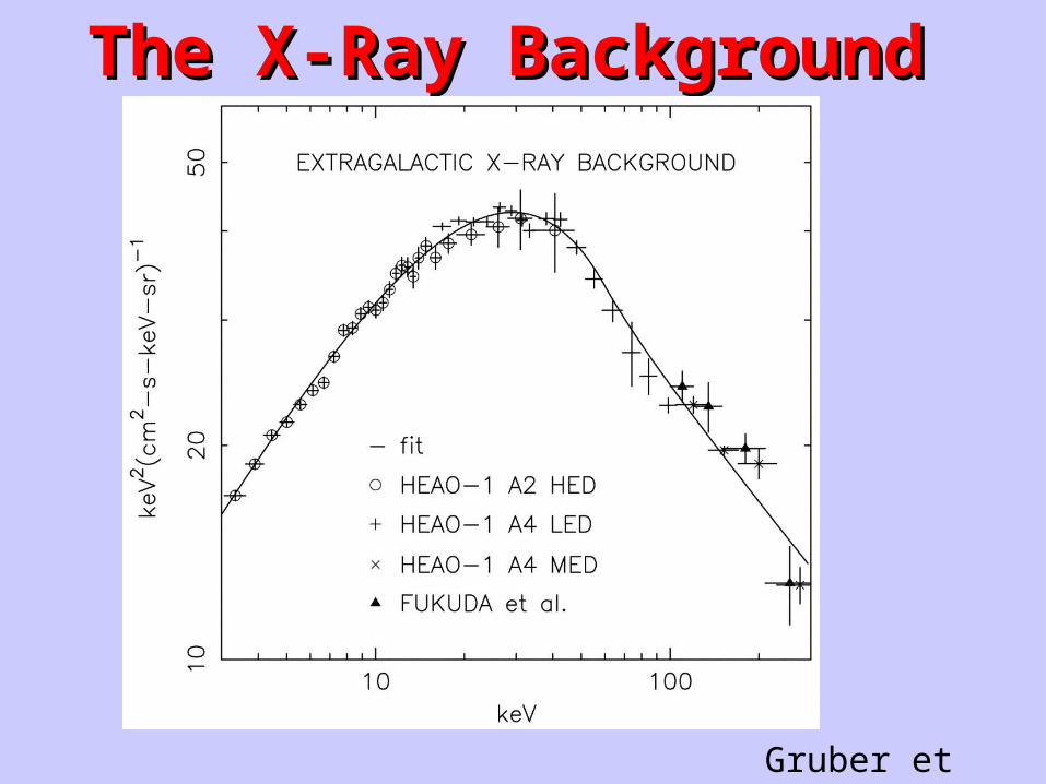
The X-Ray BackgroundThe X-Ray Background
Gruber et al. 1999
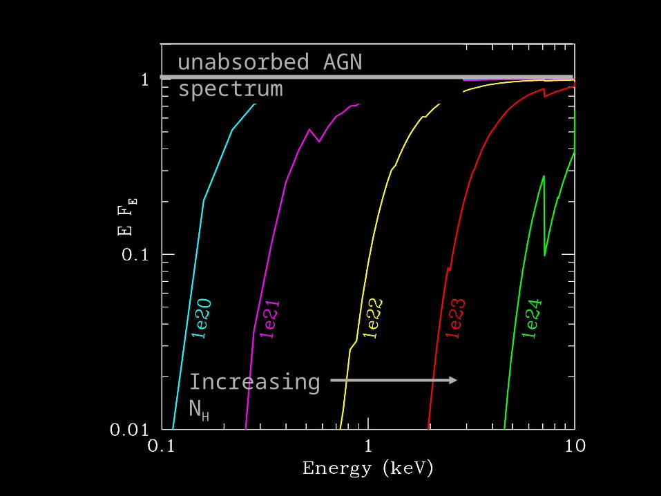
unabsorbed AGN spectrum
Increasing NH
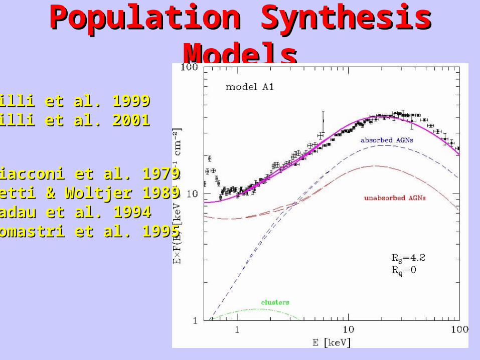
Population Synthesis ModelsPopulation Synthesis Models
Gilli et al. 1999Gilli et al. 1999Gilli et al. 2001Gilli et al. 2001
Giacconi et al. 1979Giacconi et al. 1979Setti & Woltjer 1989Setti & Woltjer 1989Madau et al. 1994Madau et al. 1994Comastri et al. 1995Comastri et al. 1995

Hasinger 2002
Gilli et al. population synthesis predictions
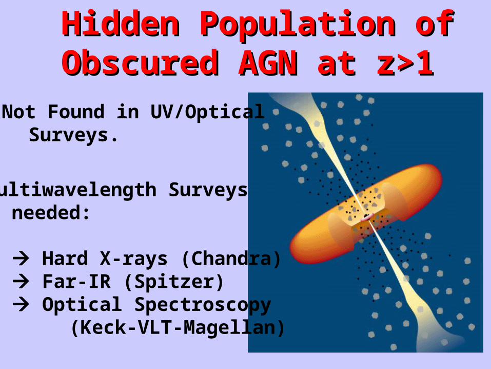
Hidden Population of Hidden Population of Obscured AGN at z>1Obscured AGN at z>1
Not Found in UV/Optical Surveys.
Multiwavelength Surveys needed:
Hard X-rays (Chandra) Far-IR (Spitzer) Optical Spectroscopy (Keck-VLT-Magellan)

GOODSGOODSdesigned to find designed to find
obscured AGN obscured AGN at the quasar epoch, at the quasar epoch, z~2-3z~2-3
Chandra Deep Fields, Spitzer Legacy, HST Treasury (3.5+ Msec) (800 hrs) (600 hrs) (3.5+ Msec) (800 hrs) (600 hrs)
Very deep imagingVery deep imaging~70 times HDF area (0.1 deg~70 times HDF area (0.1 deg22))
Extensive follow-up spectroscopy (VLT, Gemini, …)Extensive follow-up spectroscopy (VLT, Gemini, …)

B = 27.2
V = 27.5
i = 26.8
z = 26.7
B = 27.9
V = 28.2
I = 27.6
∆m ~ 0.7-0.8AB mag; S/N=10Diffuse source, 0.5” diameterAdd ~ 0.9 mag for stellar sources
ACS WFPC2

GOODS X-Ray SourcesGOODS X-Ray Sources
Chandra Deep Field North: Chandra Deep Field North:
Chandra Deep Field South: Chandra Deep Field South:
2 Ms2 Ms 503 sources503 sources 1.4x101.4x10-16 -16 ergs cmergs cm-2-2ss-1-1 (2-8 keV) (2-8 keV)
1 Ms1 Ms 326 sources326 sources 4.5x104.5x10-16 -16 ergs cmergs cm-2-2ss-1-1 (2-8 keV) (2-8 keV)

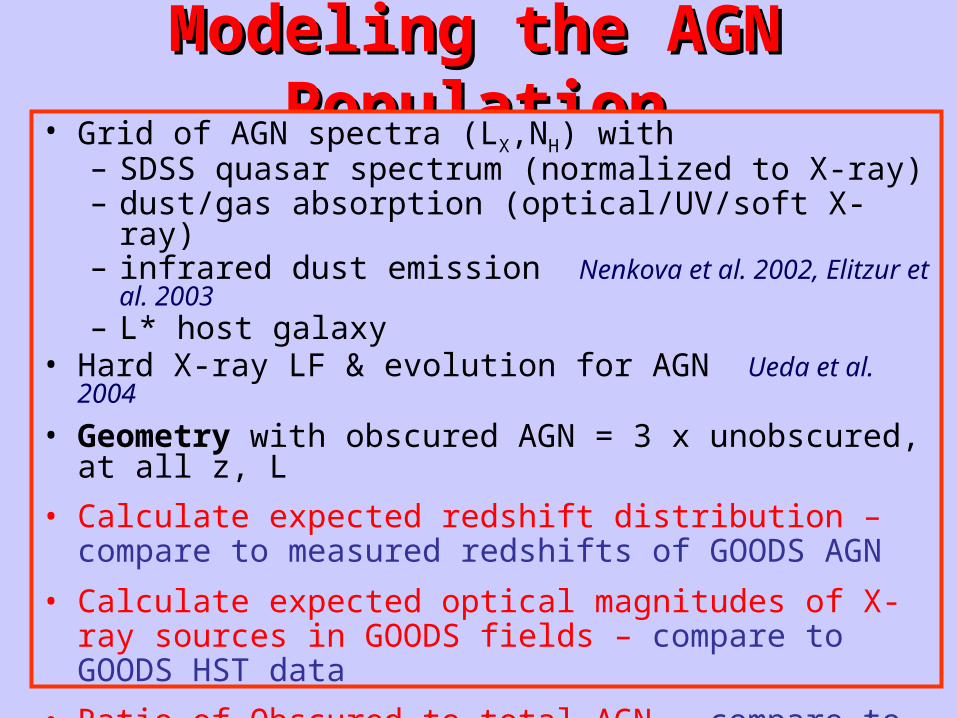
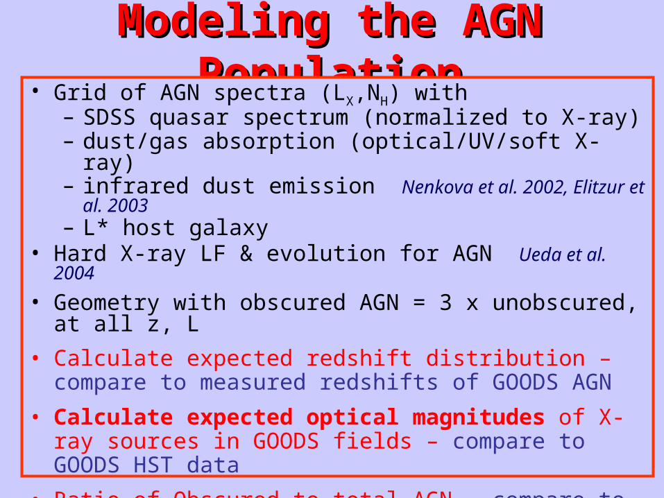
Modeling the AGN PopulationModeling the AGN Population• Grid of AGN spectra (LX,NH) with
– SDSS quasar spectrum (normalized to X-ray)– dust/gas absorption (optical/UV/soft X-ray) – infrared dust emission Nenkova et al. 2002, Elitzur et al. 2003– L* host galaxy
• Hard X-ray LF & evolution for AGN Ueda et al. 2004
• Geometry with obscured AGN = 3 x unobscured, at all z, L
• Calculate expected redshift distribution – compare to measured redshifts of GOODS AGN
• Calculate expected optical magnitudes of X-ray sources in GOODS fields – compare to GOODS HST data
• Ratio of Obscured to total AGN – compare to reported trends
• Calculate expected N(S) for infrared sources – compare to GOODS Spitzer data
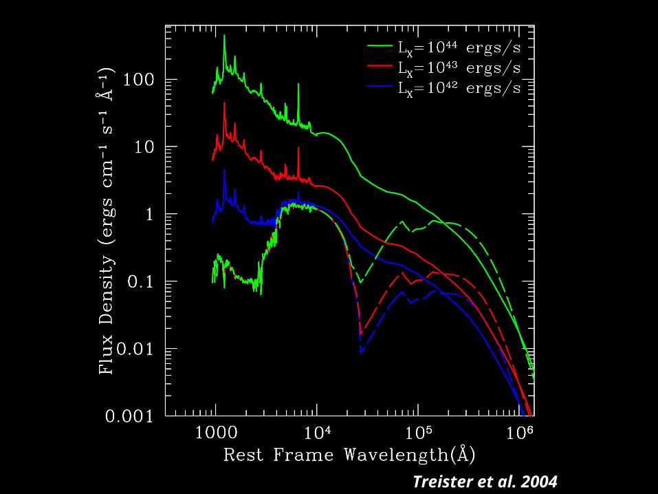
Treister et al. 2004
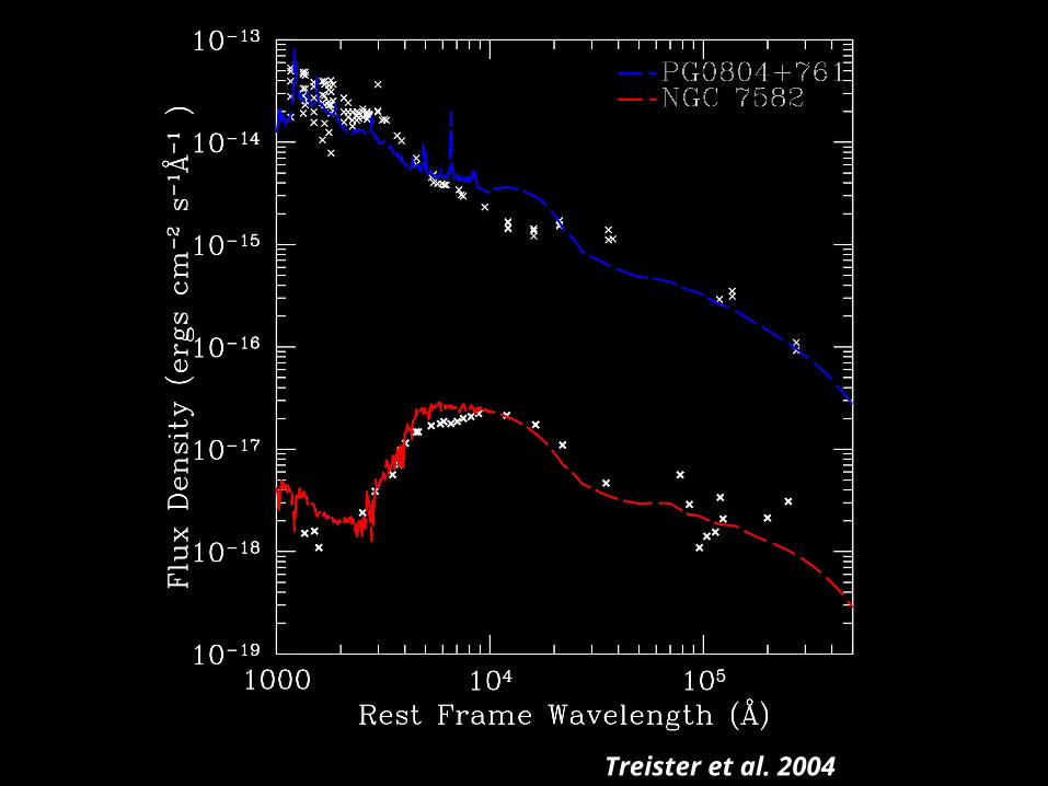
Treister et al. 2004

Modeling the AGN PopulationModeling the AGN Population• Grid of AGN spectra (LX,NH) with
– SDSS quasar spectrum (normalized to X-ray)– dust/gas absorption (optical/UV/soft X-ray) – infrared dust emission Nenkova et al. 2002, Elitzur et al. 2003– L* host galaxy
• Hard X-ray LF & evolution for AGN Ueda et al. 2004
• Geometry with obscured AGN = 3 x unobscured, at all z, L
• Calculate expected redshift distribution – compare to measured redshifts of GOODS AGN
• Calculate expected optical magnitudes of X-ray sources in GOODS fields – compare to GOODS HST data
• Ratio of Obscured to total AGN – compare to reported trends
• Calculate expected N(S) for infrared sources – compare to GOODS Spitzer data
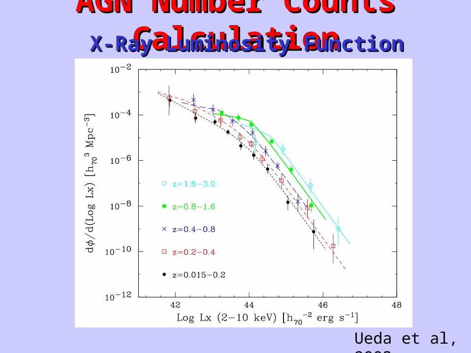
AGN Number Counts CalculationAGN Number Counts CalculationX-Ray Luminosity FunctionX-Ray Luminosity Function
Ueda et al, 2003
Modeling the AGN PopulationModeling the AGN Population• Grid of AGN spectra (LX,NH) with
– SDSS quasar spectrum (normalized to X-ray)– dust/gas absorption (optical/UV/soft X-ray) – infrared dust emission Nenkova et al. 2002, Elitzur et al. 2003– L* host galaxy
• Hard X-ray LF & evolution for AGN Ueda et al. 2004
• Geometry with obscured AGN = 3 x unobscured, at all z, L
• Calculate expected redshift distribution – compare to measured redshifts of GOODS AGN
• Calculate expected optical magnitudes of X-ray sources in GOODS fields – compare to GOODS HST data
• Ratio of Obscured to total AGN – compare to reported trends
• Calculate expected N(S) for infrared sources – compare to GOODS Spitzer data

Dust emission models from Nenkova et al. 2002, Elitzur et al. 2003
Simplest dust distribution that satisfies
NH = 1020 – 1024 cm-2
3:1 ratio (divide at 1022 cm-2)Random angles NH distribution

Modeling the AGN PopulationModeling the AGN Population• Grid of AGN spectra (LX,NH) with
– SDSS quasar spectrum (normalized to X-ray)– dust/gas absorption (optical/UV/soft X-ray) – infrared dust emission Nenkova et al. 2002, Elitzur et al. 2003– L* host galaxy
• Hard X-ray LF & evolution for AGN Ueda et al. 2004
• Geometry with obscured AGN = 3 x unobscured, at all z, L
• Calculate expected redshift distribution – compare to measured redshifts of GOODS AGN
• Calculate expected optical magnitudes of X-ray sources in GOODS fields – compare to GOODS HST data
• Ratio of Obscured to total AGN – compare to reported trends
• Calculate expected N(S) for infrared sources – compare to GOODS Spitzer data
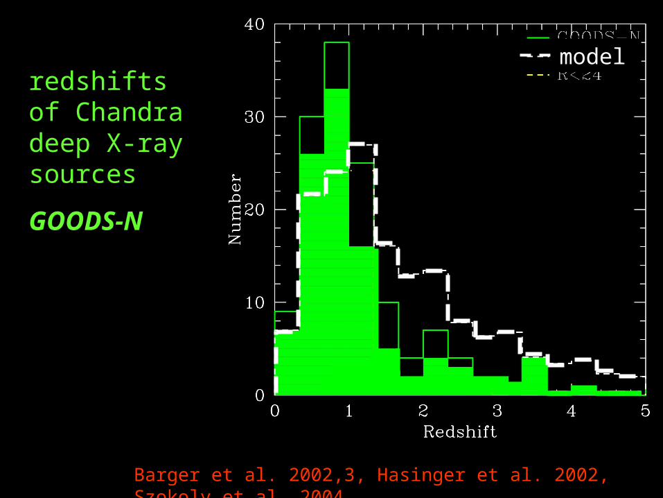
redshifts of Chandra deep X-ray sources
GOODS-N
Barger et al. 2002,3, Hasinger et al. 2002, Szokoly et al. 2004
model
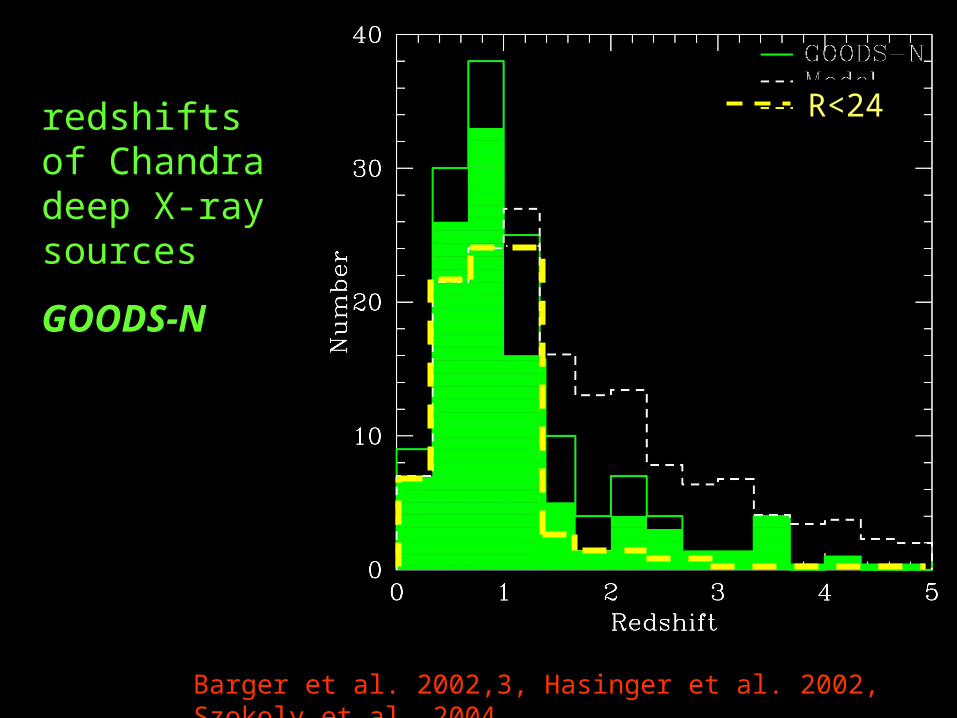
redshifts of Chandra deep X-ray sources
GOODS-N
Barger et al. 2002,3, Hasinger et al. 2002, Szokoly et al. 2004
R<24

Treister et al. 2004
redshifts of Chandra deep X-ray sources
GOODS-S

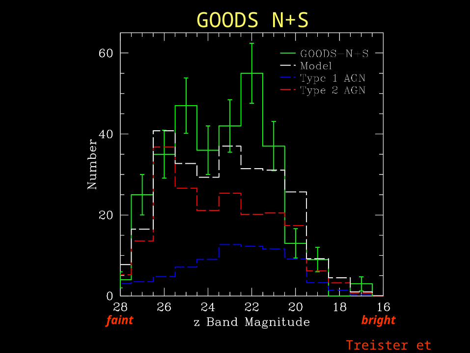
GOODS N+S DistributionGOODS N+S Distribution
Treister et al, 2004

CYDER X-ray/optical survey
Treister, et al 2004

SEXSI X-ray/optical survey
Harrison, Helfand, et al.
Modeling the AGN PopulationModeling the AGN Population• Grid of AGN spectra (LX,NH) with
– SDSS quasar spectrum (normalized to X-ray)– dust/gas absorption (optical/UV/soft X-ray) – infrared dust emission Nenkova et al. 2002, Elitzur et al. 2003– L* host galaxy
• Hard X-ray LF & evolution for AGN Ueda et al. 2004
• Geometry with obscured AGN = 3 x unobscured, at all z, L
• Calculate expected redshift distribution – compare to measured redshifts of GOODS AGN
• Calculate expected optical magnitudes of X-ray sources in GOODS fields – compare to GOODS HST data
• Ratio of Obscured to total AGN – compare to reported trends
• Calculate expected N(S) for infrared sources – compare to GOODS Spitzer data
Treister et al. 2004
brightfaint
GOODS N+S

Modeling the AGN PopulationModeling the AGN Population• Grid of AGN spectra (LX,NH) with
– SDSS quasar spectrum (normalized to X-ray)– dust/gas absorption (optical/UV/soft X-ray) – infrared dust emission Nenkova et al. 2002, Elitzur et al. 2003– L* host galaxy
• Hard X-ray LF & evolution for AGN Ueda et al. 2004
• Geometry with obscured AGN = 3 x unobscured, at all z, L
• Calculate expected redshift distribution – compare to measured redshifts of GOODS AGN
• Calculate expected optical magnitudes of X-ray sources in GOODS fields – compare to GOODS HST data
• Ratio of Obscured to total AGN – compare to reported trends
• Calculate expected N(S) for infrared sources – compare to GOODS Spitzer data
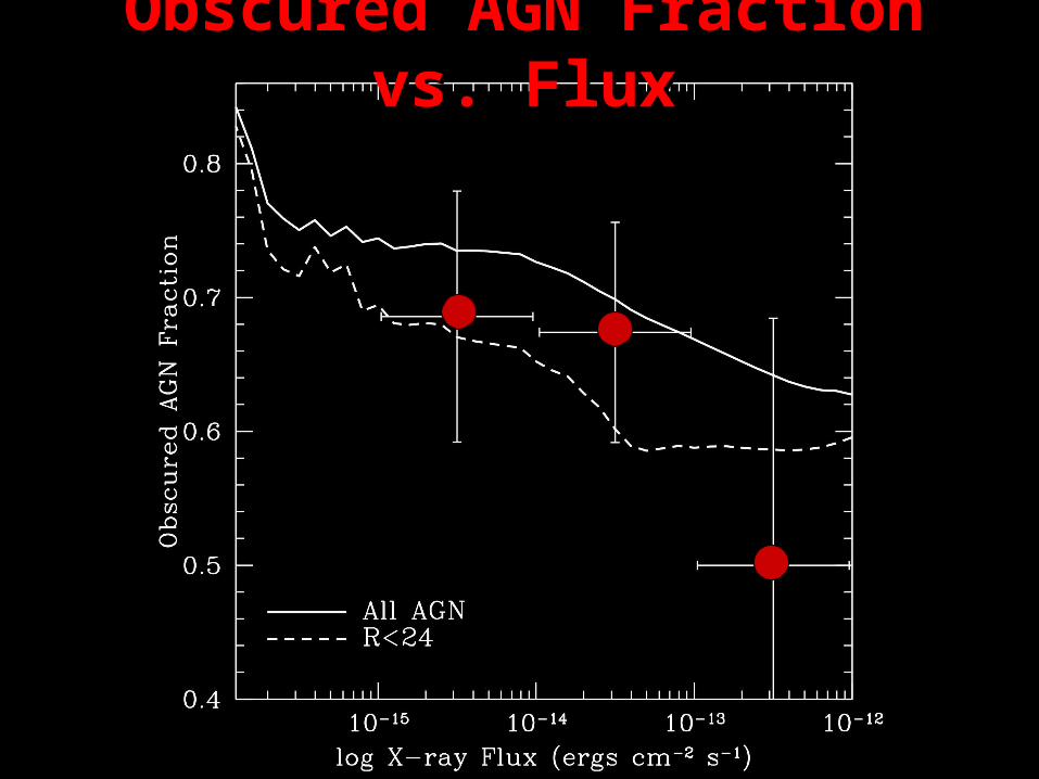
Obscured AGN Fraction vs. FluxObscured AGN Fraction vs. Flux
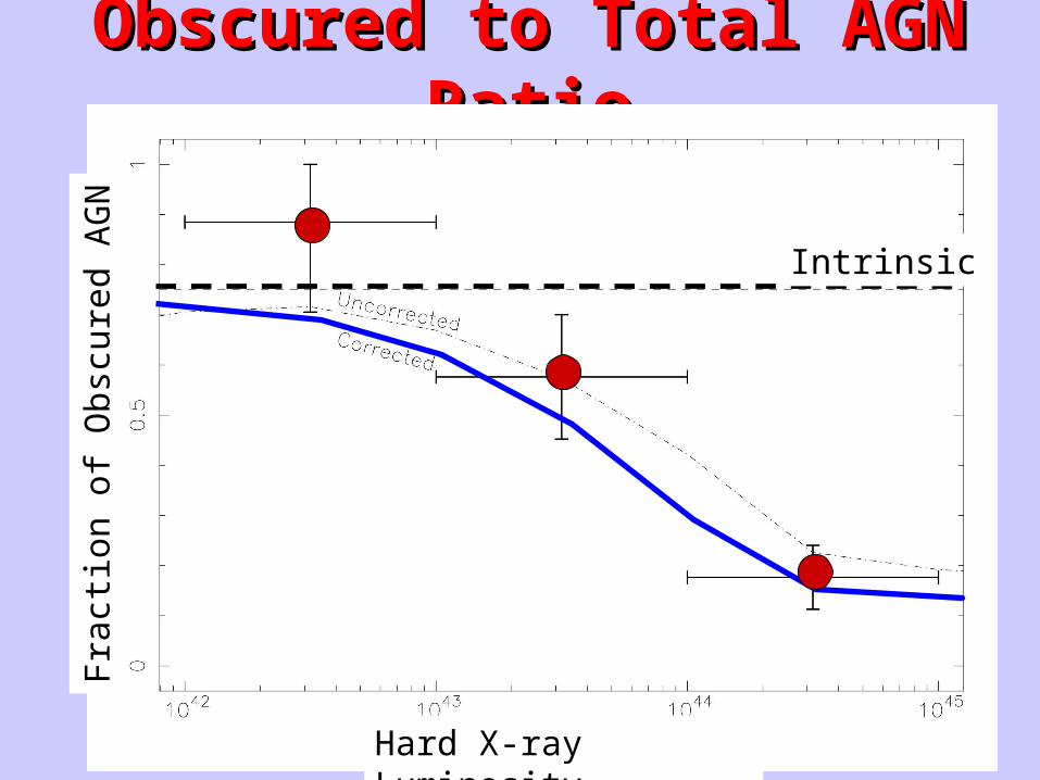
Obscured to Total AGN RatioObscured to Total AGN RatioF
ract
ion
of O
bscu
red
AG
N Intrinsic
Hard X-ray Luminosity
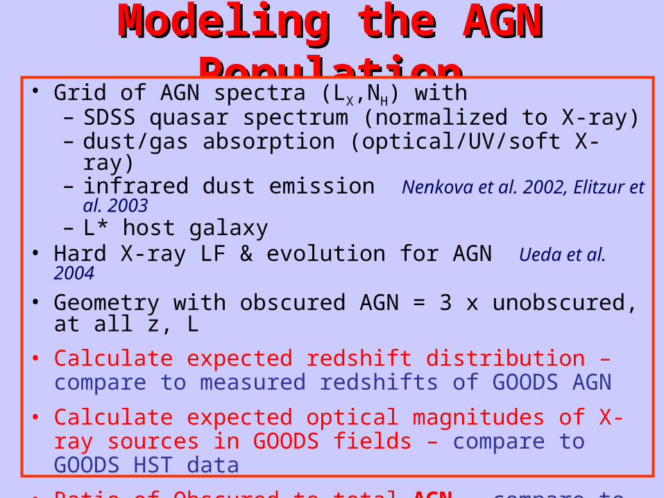
Modeling the AGN PopulationModeling the AGN Population• Grid of AGN spectra (LX,NH) with
– SDSS quasar spectrum (normalized to X-ray)– dust/gas absorption (optical/UV/soft X-ray) – infrared dust emission Nenkova et al. 2002, Elitzur et al. 2003– L* host galaxy
• Hard X-ray LF & evolution for AGN Ueda et al. 2004
• Geometry with obscured AGN = 3 x unobscured, at all z, L
• Calculate expected redshift distribution – compare to measured redshifts of GOODS AGN
• Calculate expected optical magnitudes of X-ray sources in GOODS fields – compare to GOODS HST data
• Ratio of Obscured to total AGN – compare to reported trends
• Calculate expected N(S) for infrared sources – compare to GOODS Spitzer data

Predicted Spitzer counts (3.6 Predicted Spitzer counts (3.6 m)m)
~1/2 AGN missing from deep Chandra samples
Will be detected with Spitzer IRAC

Total # infrared sources in GOODS: prediction=observed
Observed distribution of infrared fluxes matches prediction.
Spitzer supports model of obscured AGNSpitzer supports model of obscured AGN
Treister, Urry, van Duyne, et al. 2004
3.6 m flux (mJy)
N(>
S)
Observed IRAC fluxes of CDF X-ray sources

ConclusionsConclusions• Simple unification model explains:
– (faint) optical magnitude distribution– redshift distribution
• This model is consistent with predictions by XRB population synthesis models:
- Broader redshift distribution with peak at z~1.3 - Type 2/Type 1~3• Observed relation between obscured AGN fraction
and X-ray luminosity can be explained as a selection effect
• GOODS Spitzer observations will put strong constrains on these models and the ratio of obscured to unobscured AGN.


