Munich Personal RePEc Archive Government interventions in banking crises: Assessing alternative schemes in a banking model of debt overhang Diemo Dietrich and Achim Hauck Halle Institute for Economic Research, Heinrich Heine University Duesseldorf 2010 Online at https://mpra.ub.uni-muenchen.de/24508/ MPRA Paper No. 24508, posted 23. August 2010 02:23 UTC
Transcript
MPRAMunich Personal RePEc Archive
Government interventions in bankingcrises: Assessing alternative schemes in abanking model of debt overhang
Diemo Dietrich and Achim Hauck
Halle Institute for Economic Research, Heinrich Heine UniversityDuesseldorf
2010
Online at https://mpra.ub.uni-muenchen.de/24508/MPRA Paper No. 24508, posted 23. August 2010 02:23 UTC
Wirtschaftswissenschaftliche Fakultät Department of Business Administration
and Economics
Government Interventions in Banking Crises: Assessing Alternative Schemes in a Banking Model of Debt Overhang
Diemo Dietrich Achim Hauck
Diskussionspapierzur Volkswirtschaftslehre, Finanzierung und Besteuerung Nr. 3/2010
Discussion Paper on Economics, Finance, and Taxation No. 3/2010
Diese Diskussionspapierreihe ist im Internet im PDF-Format unter der Adresse www.vwl-neyer.uni-duesseldorf.de/forschung/diskussionspapiere verfügbar. Sie wird gemeinsam herausgegeben von:
This Discussion Paper Series is available online in PDF format at www.vwl-neyer.uni-duesseldorf.de/Englisch/forschung/discussionpapers and is jointly edited by:
Prof. Dr. Christoph J. Börner*Tel.: +49 (0)211-81-15258 Fax: +49 (0)211-81-15316 E-Mail: [email protected]
Prof. Dr. Albrecht F. Michler*Tel.: +49(0)211-81-15372 Fax: +49(0)211-81-10434 E-Mail: [email protected]
Prof. Dr. Raimund Schirmeister*Tel.: +49(0)211-81-14655 Fax: +49(0)211-81-15157 E-Mail: [email protected]
Prof. Dr. Guido Förster*Tel.: +49 (0)211-81-10603 Fax: +49 (0)211-81-10624 E-Mail: [email protected]
Prof. Dr. Ulrike Neyer*Tel.: +49(0)211-81-11511 Fax: +49(0)211-81-12196 E-Mail: [email protected]
Prof. Dr. Heinz-Dieter Smeets*Tel.: +49-(0)211-81-15286 Fax: +49-(0)211-81-15261 E-Mail: [email protected]
*Adresse:Heinrich-Heine-Universität Düsseldorf Wirtschaftswissenschaftliche Fakultät Universitätsstraße 1 40225 Düsseldorf Deutschland
*Address:Heinrich-Heine-University Dusseldorf Department of Business Administration and Economics Universitaetsstrasse 1 40225 Dusseldorf Germany
Bei Nachfragen zu dieser Diskussionspapierreihe wenden Sie sich bitte an die derzeitige Koordinatorin: Prof. Dr. Ulrike Neyer.
Please direct any enquiries to the current coordinator: Prof. Dr. Ulrike Neyer.
Anmerkung: Beiträge zu dieser Diskussionspapierreihe sind vorläufige Papiere, die zur Diskussion und zu kritischen Anmerkungen anregen sollen. Die Analyse und Ergebnisse sind die des Autors (der Autoren) des jeweiligen Beitrages und spiegeln nicht unbedingt die Meinung anderer Mitglieder der Wirtschaftswissenschaftlichen Fakultät der Heinrich-Heine-Universität Düsseldorf wider. Jede Reproduktion als Ganzes oder in Teilen in Form einer anderen Veröffentlichung, ob in gedruckter oder elektronischer Form, ist nur mit der schriftlichen Zustimmung des Autors/der Autoren erlaubt.
Note: Papers in this Discussion Paper Series are preliminary materials circulated to stimulate discussion and critical comment. The analysis and conclusions set forth are those of the author(s) and do not indicate concurrence by other members of the Department of Business Administration and Economics at the Heinrich-Heine-University Dusseldorf. Any reproduction in the form of a different publication, whether printed or produced electronically, in whole or in part, is permitted only with the written authorisation of the author(s).
Government Interventions in Banking Crises: Assessing
Alternative Schemes in a Banking Model of Debt Overhang
Diemo Dietrich∗ Achim Hauck†
April 16, 2010
Abstract
We evaluate policy measures to stop the fall in loan supply following a banking crisis.
We apply a dynamic framework in which a debt overhang induces banks to curtail lending
or to choose a fragile capital structure. Government assistance conditional on new banking
activities, like on new lending or on debt and equity issues, allows banks to influence the scale
of the assistance and to externalize risks, implying overinvestment or excessive risk taking or
both. Assistance granted without reference to new activities, like establishing a bad bank, does
not generate adverse incentives but may have higher fiscal costs.
Keywords Banking crisis, debt overhang, bank lending, capital structure.
JEL Classification G01, G21, G28
∗Corresponding author: Halle Institute for Economic Research, 06017 Halle (Saale), Germany, Email:
[email protected], and Martin Luther University Halle-Wittenberg.†Heinrich-Heine-University Duesseldorf, Department of Economics, Universitaetsstrasse 1, 40225 Duesseldorf, Ger-
The recent financial crisis has led to large devaluations of assets which have eroded the capital basis
of banks. As a consequence, many banks have suffered from a debt overhang as it forms an obstacle
to raising fresh funds for new businesses. In this paper, we evaluate different policy measures to
stop the fall in bank loan supply following a banking crisis.
Starting with Myers (1977), it has been argued in the corporate finance literature that a debt-
laden firm may be unable to raise further funds, even for projects with positive NPV. As regards
banks, a debt overhang is special because, in contrast to nonbanks, a default on pre-existing short-
term debt may trigger a bank run.1 Such a bank run, however, creates externalities not only because
new lending of a single bank is impeded. It may also result in a systemic failure.2 Both effects
have determined much of the real costs of past banking crises (Dell’Ariccia et al, 2008). Policy
makers, therefore, face a set of interrelated problems. One is to deal with the inability of banks
to finance new valuable investment projects. Another is to prevent systemic spillover effects that
impend when an important financial institution fails. Finally, for a measure being sustainable, banks
should be assisted in a way that does not encourage further excessive risk taking.
In order to evaluate the effectiveness of different policy measures, we apply a dynamic model
in which a sudden illiquidity of (some) assets causes a debt overhang for banks. A bank responds
either by curtailing new loans or by choosing a fragile capital structure, a feature that many banking
crises have shared (Laeven and Valencia, 2008). We argue that government assistance conditional on
new banking activities allows banks to influence the scale of the assistance and to externalize risks,
which results in excessive risk taking or overinvestment or both. By contrast, granting assistance
without reference to new activities does not generate these adverse incentives.
These results are derived from a banking model based on work by Diamond and Rajan (2000,
2001). They argue that a banker has an informational advantage in collecting loans and that this
advantage allows her to extract an information rent. Deposits are useful to prevent such rent extrac-
tion. They serve as a commitment device because depositors will run on the bank whenever a banker
is suspected to misbehave. When asset values are risky, however, deposits imply that a bank would
sometimes be run even without any misbehavior of the banker. Therefore, a banker will also issue
non-deposit debt or equity shares, which serve as a buffer in bad times but allow her to withhold
some rents in good times.
In this setting, we consider a banker who has to repay outstanding deposits at some date. In the
past, these deposits have been used to refinance bank assets. These assets, however, have turned out
to be non-performing. Their market liquidity has dried up so that selling them does not generate any
immediate return. Funding liquidity is also weak. The reason here is that a banker cannot borrow
1This aspect has largely been neglected so far. For example, although dedicated to banks, the analysis by Philippon
and Schnabl (2009) is applicable to non-financial and financial firms alike.2Systemic risks may stem from contractual linkages (Allen and Gale, 2000), from identification problems in funding
markets (Freixas et al, 2000), from a liquidity-solvency spiral (Diamond and Rajan, 2005), or because shocks are common
to all banks (Acharya, 2009). The specific reason for systemic risks is not explicitly considered here. Instead, we take the
existence of systemically important bank liabilities and the need to protect them as granted.
4
against the full future value of non-performing assets, because their returns are uncertain, so that
the banker, to some extent, relies on non-deposit debt or equity shares. As a result, the bank may be
insolvent if outstanding deposits are too large compared to what the banker can raise by borrowing
against non-performing assets.
These liquidity and solvency problems for a bank form an obstacle to new business loans and to
bank stability. Stability of the bank not only requires to serve outstanding deposits but also to issue
only little new deposits as the prospective asset returns are uncertain. Though non-deposit debt and
equity shares buffer against this risk, they do not allow the banker to raise much because of their
lacking disciplinary effect. Hence, the higher the volume of outstanding deposits, the more limited
is new lending when the banker wants to keep the bank stable. When the banker chooses to issue
more new deposits, she opts for a fragile capital structure and puts the existence of the bank at risk,
but at least can commit to repay more if everything goes well. This commitment eases the funding
constraint for new loans, although it is associated with financial instability.
How do different policy measures influence a bank’s lending behavior, capital structure and risk
taking in this situation? We consider deposit guarantees, capital injections, and bad banks.3 We
argue that although government interventions are needed to mitigate the externalities of a debt over-
hang, success crucially depends on their terms. When the goal is to re-establish the intermediation
function of banks in order to reduce shortages in the supply of new loans and to restore financial sta-
bility, government should not support new banking activities, neither directly nor indirectly. Instead,
government should assume the overhanging debt of banks. The reason is that different measures of
subsidizing banks in their efforts to raise new funds will in many cases result in overinvestment
and in financial fragility. Government intervention may result in future instability of the bank, not
because of incentives for banks to take excessive risk in anticipation of a future bailout (as in Nier
and Baumann, 2006; Panageas, 2010). We exclude repeated bailouts. Instead, excessive risk taking
may occurs because overinvestment and financial fragility are interlinked. When banks are incited
to overinvest, they have to raise more funds. As the marginal source of funding is deposits, banks
issue more deposits than compatible with safety.
Based upon these insights, we uncover the underlying, more general problem with government
interventions in banking crises. The debt overhang, which hampers new business lending, is the
result of past lending behavior and capital structure decisions. In order to release new lending from
the debt burden, government could either cope with the existing debt or support new lending. These
two options are not equivalent, however. Only with the first option, government does not make its
financial assistance depending on new contracts, and thus does not incite banks to externalize risks
that lead to excessive risk taking and overinvestment.
By exploring the effects of a bank capital crunch on loan supply, this paper is related to Peek and
Rosengren (1995) and Holmstrom and Tirole (1997). In contrast to these studies, however, we also
focus on the question of how policy measures should be shaped in order to mitigate the real costs
3Monetary policy measures are excluded from the analysis. Although these measure are helpful in overcoming pure
liquidity problems, they can at best collaterally support fiscal measures in the presence of insolvency problems, see
Diamond and Rajan (2005).
5
of banking crises. Moreover, while Holmstrom and Tirole (1997) conclude that a recapitalization
of banks with taxpayer money can improve banks’ incentive to monitor loans, we argue that this
may also imply excessive risk taking and overinvestment. Diamond (2001), Demirguc-Kunt and
Detragiache (2002), and Flannery (2009) study the effects of single policy measures but do not
compare them as we do in this paper. Aghion et al (1999) and Mitchell (2001), who compare
different policy measures, do not consider the dynamic linkage between bank lending and capital
structure.
The paper is organized as follows. In section 2, we present the benchmark model. In section 3,
we fit some recently applied policy instruments in the model in order to analyze their likely effects
on bank lending and risk taking. In section 4 we further discuss the results and in section 5 we
briefly summarize our findings.
2 A banking model of debt overhang
2.1 Agents and technologies
We consider a bank that is run by a banker. While the banker has no funds on her own, there are
many investors endowed with plenty of funds. All agents are risk neutral and have access to a safe
investment opportunity with a zero rate of return.
At date t, the banker has to repay outstanding deposits D0. In the past, these deposits were
used to originate loans supposed to be collected at t. However, in the meantime the economic
environment has worsened unexpectedly and these legacy assets have turned out to generate nothing
at t. Some assets are completely written off, others only delay. The latter will earn an uncertain
return at date t + 1 if the bank survives until then. With probability p, the economy has recovered
at t + 1 and legacy assets pay xg > 0 at this date. If the economy fails to turn upward again (with
probability 1− p), the return will be only xb ∈ [0,xg).Also at t, the banker faces new lending opportunities. Let L denote the volume of new business
loans. They will earn RL at t +1 if the economy recovers and nothing otherwise. With pR ∈ (1,2),expected returns per unit of new loans cover the initial outlay but are not too large. The banker can
also invest C in a safe asset, which will pay C at t +1.
For all bank assets to generate a return, specific skills are required. Investors do not have these
skills so that only the banker can collect loans and other bank assets (Diamond and Rajan, 2001).
Maintaining these collection skills causes private costs to the banker. Managing the safe asset is
not very demanding, and the costs of managing old loans are predetermined at date t. Hence, the
variable costs for these two asset classes are negligible. By contrast, the more new loans the banker
grants the more complex and demanding the task of managing them will be. Total costs c(L) are thus
an increasing and convex function of L with c(0) = c′(0) = 0 and c′′(L) > 0. These costs are non-
verifiable. The first-best lending volume L f b : pR−1 = c′(L f b) is thus unknown to an outside third
6
party, so that although a supervisor can observe the actual lending volume, it cannot tell whether it
is the efficient one.4
2.2 Bank capital structure
The banker has an informational advantage in collecting the returns on bank assets. This advantage
gives her some leeway to renegotiate contractual payments to investors by threatening to withdraw
her skills. The extent to which the banker can renegotiate ex post, and thus the banker’s ability to
raise funds ex ante, depends on the bank’s capital structure.
Deposits serve as a commitment device for a banker (Diamond and Rajan, 2001). They are
payable on demand based on a first-come-first-served principle. If the banker tried to renegotiate
deposits, every single depositor would run on the bank and demand the liquidation of assets until
being fully paid. Since assets are assumed to have (almost) no liquidation value, a run destroys the
value of the bank. It is the threat of being run that effectively prevents the banker from renegoti-
ating with depositors. The disadvantage of deposits is that they cannot be renegotiated even when
the value of the bank’s assets slumps down for reasons outside the banker’s control. A bank run,
although inefficient, cannot be avoided then.
The banker can also issue non-deposit debt and equity shares. Both claims are junior to deposits
and not subject to a first-come-first-served constraint. Hence, debt and equity can be renegotiated by
the banker in bad times and thus act as a buffer against low loan earnings. However, the banker can
threaten to withhold her skills when the total value of loans, legacy assets, and the safe asset exceeds
deposits. This threat allows her to extract a personal rent. Adapting the approach of Diamond and
Rajan (2000), shareholders and debtholders could force the banker to pay them half of the returns
on all bank assets net of deposits. Hence, the banker can pledge to them only a share λ ≤ 0.5 of
her earnings net of deposits and diverts the remaining share 1− λ . The ability to extract a rent
at t + 1 eventually restricts the amount of funds she can raise at t.5 Abusing terminology slightly,
we henceforth refer to both, the holders of equity shares and the holders of non-deposit debt as
shareholders.
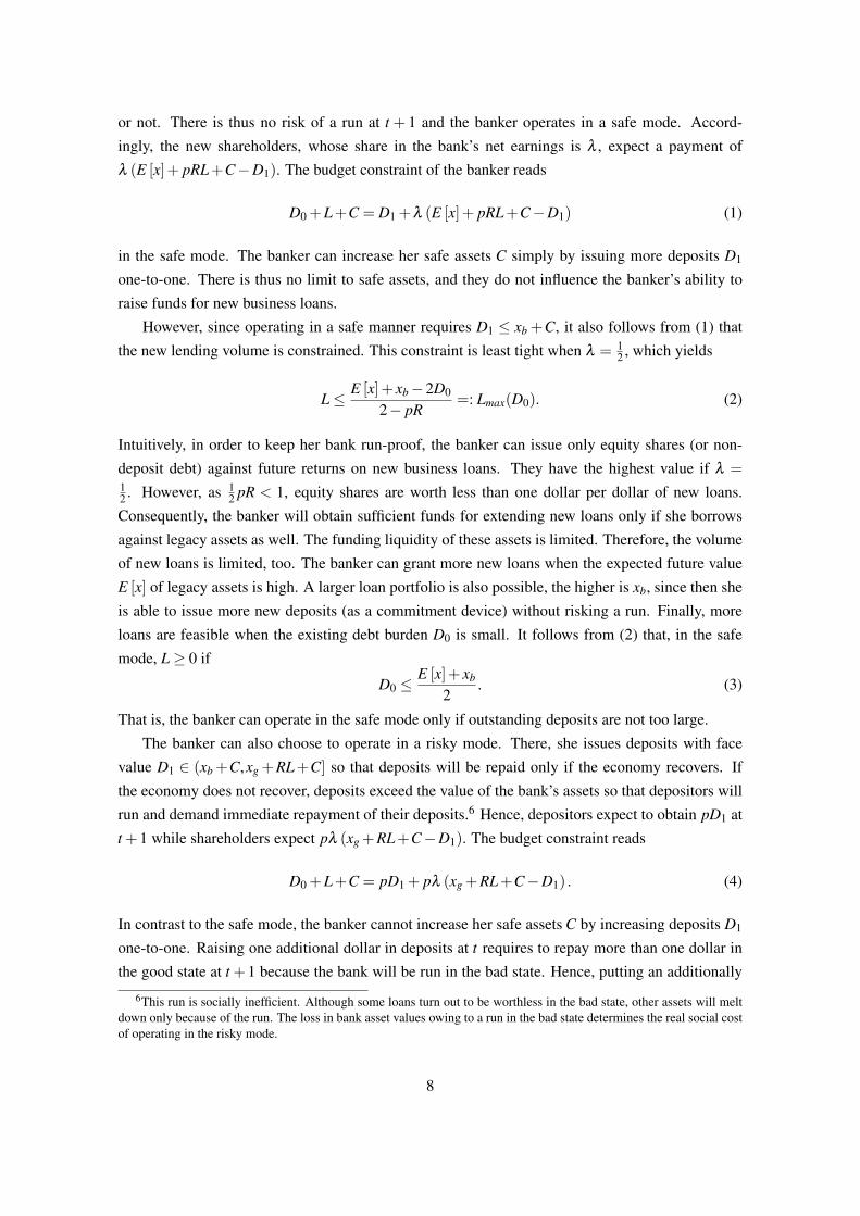
2.3 Restrictions on bank loan supply
The banker can avoid an immediate run at t only by repaying the existing deposits D0. Accordingly,
if she plans to extend new loans L and to hold some amount C in the safe asset, the banker needs to
raise a total of D0 +L+C at t.
The liquidity that a banker can raise at t is limited to the amount she can borrow against prospec-
tive asset values at this date. Let D1 denote the face value of new deposits issued at t. If D1≤ xb +C,
the banker is able to repay D1 to new depositors at t +1 irrespective whether the economy recovers
4Assuming that not only new loans and legacy assets but also safe assets require specific skills is not necessary for our
results to hold. However, treating all assets symmetrically reduces complexity.5If λ = 0.5, the banker issues equity shares with shareholders being always repaid half of the asset returns net of
deposits. If λ < 0.5, the banker issues non-deposit debt with debtholders being repaid either some fixed amount or at
most half of the asset returns net of deposits, depending on which amount is smaller.
7
or not. There is thus no risk of a run at t + 1 and the banker operates in a safe mode. Accord-
ingly, the new shareholders, whose share in the bank’s net earnings is λ , expect a payment of
λ (E [x]+ pRL+C−D1). The budget constraint of the banker reads
D0 +L+C = D1 +λ (E [x]+ pRL+C−D1) (1)
in the safe mode. The banker can increase her safe assets C simply by issuing more deposits D1
one-to-one. There is thus no limit to safe assets, and they do not influence the banker’s ability to
raise funds for new business loans.
However, since operating in a safe manner requires D1 ≤ xb +C, it also follows from (1) that
the new lending volume is constrained. This constraint is least tight when λ = 12, which yields
L≤ E [x]+ xb−2D0
2− pR=: Lmax(D0). (2)
Intuitively, in order to keep her bank run-proof, the banker can issue only equity shares (or non-
deposit debt) against future returns on new business loans. They have the highest value if λ =12. However, as 1
2pR < 1, equity shares are worth less than one dollar per dollar of new loans.
Consequently, the banker will obtain sufficient funds for extending new loans only if she borrows
against legacy assets as well. The funding liquidity of these assets is limited. Therefore, the volume
of new loans is limited, too. The banker can grant more new loans when the expected future value
E [x] of legacy assets is high. A larger loan portfolio is also possible, the higher is xb, since then she
is able to issue more new deposits (as a commitment device) without risking a run. Finally, more
loans are feasible when the existing debt burden D0 is small. It follows from (2) that, in the safe
mode, L≥ 0 if
D0 ≤ E [x]+ xb
2. (3)
That is, the banker can operate in the safe mode only if outstanding deposits are not too large.
The banker can also choose to operate in a risky mode. There, she issues deposits with face
value D1 ∈ (xb +C,xg +RL+C] so that deposits will be repaid only if the economy recovers. If
the economy does not recover, deposits exceed the value of the bank’s assets so that depositors will
run and demand immediate repayment of their deposits.6 Hence, depositors expect to obtain pD1 at
t +1 while shareholders expect pλ (xg +RL+C−D1). The budget constraint reads
D0 +L+C = pD1 + pλ (xg +RL+C−D1) . (4)
In contrast to the safe mode, the banker cannot increase her safe assets C by increasing deposits D1
one-to-one. Raising one additional dollar in deposits at t requires to repay more than one dollar in
the good state at t +1 because the bank will be run in the bad state. Hence, putting an additionally
6This run is socially inefficient. Although some loans turn out to be worthless in the bad state, other assets will melt
down only because of the run. The loss in bank asset values owing to a run in the bad state determines the real social cost
of operating in the risky mode.
8
raised dollar in the safe asset alone does not suffice to meet the depositors claim in the good state at
t + 1. Instead, the banker must cross-pledge earnings from new business loans, too. The safe asset
is thus detrimental to the banker’s ability to raise funds for new loans in the risky mode.
The risky mode differs from the safe mode in another important aspect. When operating in a
risky manner, a banker could issue deposits with face value R per unit of new loans. Depositors
would then expect to receive pR > 1. Accordingly, they would be willing to provide more than one
dollar per unit of new loans, implying that there is no upper bound on new business loans L in the
risky mode.
2.4 Implications
New lending is linked to the future stability of the bank. Only when new loans fulfill restriction (2),
the banker can avoid a bank run. Once the banker has decided to make new loans in a safe manner,
loans L, safe assets C, deposits D1 and the share λ are chosen to solve
Proposition 1 For a given outstanding amount of deposits D0, the banker
1. operates in a safe manner and invests according to
L∗ =
⎧⎨⎩ L f b i f D0 ≤ E[x]+xb−(2−pR)L f b
2
Lmax(D0) i f D0 ∈(
E[x]+xb−(2−pR)L f b
2,min
{D0,
E[x]+xb2
}] (7)
2. operates in a risky manner and invests according to
L∗ = L f b i f D0 ∈(
min{
D0,E[x]+xb
2
}, pxg +(pR−1)L f b− c(L f b)
](8)
3. is run already at t if D0 > pxg +(pR−1)L f b− c(L f b),
where D0 is the outstanding amount of deposits for which
[(pR−1)L f b− c(L f b)
]− [(pR−1)Lmax(D0)− c(Lmax(D0))
]= (1− p)xb. (9)
9
Proof. See appendix.
With a small outstanding amount of deposits, the banker grants loans according to the first best
and operates in a safe manner. The reason is twofold. First, the restriction on loan supply (2) is not
binding. Second, expected repayments to investors do not depend on the bank’s mode of operation
while earnings from legacy assets contribute to her rents in both states only when she opts for the
safe mode of refinancing.
With a moderate outstanding amount of deposits, restriction (2) is binding, and the banker faces
the following trade-off when deciding on the operation mode. On the one hand, operating in the
safe mode requires to cut loan supply to Lmax < L f b. This reduces the banker’s expected future loan
earnings by an amount given by the LHS of (9), with the fall in loan earnings being larger the higher
is the outstanding amount of deposits D0. On the other hand, operating in the risky mode does not
require to reduce loan supply. However, the run in the bad state, occurring with probability (1− p),implies that the return xb of the legacy assets is lost (see RHS of (9)). The banker thus decides in
favor of the safe mode and of reducing her loan supply when the safe mode is feasible (see (3))
and when underinvestment in the safe mode reduces her rents by less than the foreseeable run in
the risky mode (see (9)). When the debt overhang problem is more severe, the banker pursues the
risky strategy as long as this does not imply a negative expected profit for her. If the outstanding
amount of deposits cannot be covered by the expected asset values (net of financing and portfolio
management cost) the bank will be run already at t.
A further implication is that access to safe assets does not ease the banker’s financial constraint
with respect to new loans. In the safe mode, marginal financing costs for safe assets are equal to
their marginal returns. Hence, financing safe assets can be separated from financing risky loans so
that safe assets do not influence the lending decision of a debt-laden banking firm operating in a
safe manner. In the risky mode, safe assets are no longer safe from the perspective of depositors as
the bank has chosen a fragile capital structure. Since a run occurs with probability (1− p), marginal
returns on safe assets are only p. With new business loans being more profitable on expectation and
safe assets crowding out finance for new loans, the banker does not invest in safe assets but focuses
on new risky loans.
3 Effects of government interventions
As argued in the preceding section, unanticipated changes in the risk-return structure of bank assets
may result in a debt overhang that forces banks either to reduce new lending or to jeopardize their fi-
nancial stability. The externality created by the debt overhang, therefore, is two-dimensional and so
is the objective of government interventions. First, government should enable banks to provide the
efficient level of intermediation services. Second, in so doing, banks should not be incited to take
on excessive risks. In this section, we analyze how banks change their lending behavior and capital
structure in response to different policy measures. We consider capital injections, deposit guaran-
10
tees, and bad banks. In the 2007-09 crisis, these interventions were among the most frequently taken
measures around the globe (Praet and Nguyen, 2008; Panetta et al, 2009).
3.1 Capital injections
Capital injections can take two forms. Either the government makes the assistance conditional
on new activities of the bank, e. g., on new lending or on new equity or deposit issues. Or the
government provides taxpayer money independently of new banking activities through, e. g., lump
sum transfers or transfers conditional on the existing debt burden of a bank. Both forms of capital
injections have in common that they foster new lending only if the government does not require
the banker to fully pay them back. Otherwise they merely crowd out private funds. However, the
two forms of capital injections differ with respect to their contributions to the government’s policy
objective.
3.1.1 Unconditional on new activities
A lump sum subsidy S granted by the government to the banker is a good illustrative example
for financial assistance that is independent from new banking activities. In principle, this transfer
could be used to repay (some of) the old depositors–a straightforward way to free a bank from
its debt overhang as the government directly assumes responsibility for the outstanding deposits
D0 (or parts of it). A standard result in public finance is that a lump sum transfer does not alter
first-order conditions and is thus efficient. Hence, we expect a lump sum transfer not to change a
bankers’ investment incentives. However, as we will show, it does affect a banker’s decision on
capital structure and thus the stability of the bank.
Consider a bank which operates in a safe manner at first. If the government pays a lump sum S,
the banker’s budget constraint (1) modifies to
D0 +L+C = D1 +λ (E [x]+ pRL+C−D1)+S. (10)
This budget constraint together with D1 ≤ xb +C and λ = 12
implies
L≤ E [x]+ xb−2(D0−S)2− pR
=: Lmax(D0−S). (11)
Hence, the higher is the subsidy, the higher is the volume of new loans that is feasible if the banker
wishes to operate safely. The banker is able to make new loans in a safe manner only if
D0−S <E [x]+ xb
2. (12)
Comparing with the benchmark model in the previous section, we see that in the safe mode an
outstanding amount of deposits D0 and a subsidy S is equivalent to an outstanding amount D0− S
and no subsidy.
11
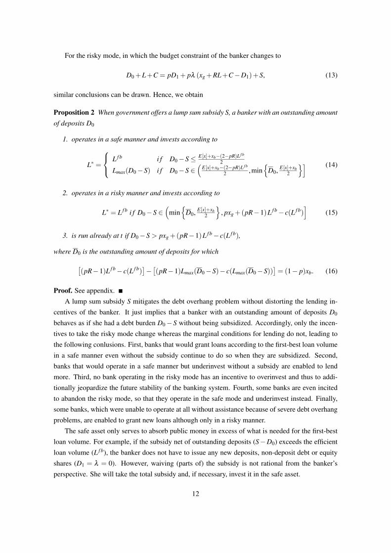
For the risky mode, in which the budget constraint of the banker changes to
D0 +L+C = pD1 + pλ (xg +RL+C−D1)+S, (13)
similar conclusions can be drawn. Hence, we obtain
Proposition 2 When government offers a lump sum subsidy S, a banker with an outstanding amount
of deposits D0
1. operates in a safe manner and invests according to
L∗ =
⎧⎨⎩ L f b i f D0−S≤ E[x]+xb−(2−pR)L f b
2
Lmax(D0−S) i f D0−S ∈(
E[x]+xb−(2−pR)L f b
2,min
{D0,
E[x]+xb2
}] (14)
2. operates in a risky manner and invests according to
L∗ = L f b i f D0−S ∈(
min{
D0,E[x]+xb
2
}, pxg +(pR−1)L f b− c(L f b)
](15)
3. is run already at t if D0−S > pxg +(pR−1)L f b− c(L f b),
where D0 is the outstanding amount of deposits for which
[(pR−1)L f b− c(L f b)
]− [(pR−1)Lmax(D0−S)− c(Lmax(D0−S))
]= (1− p)xb. (16)
Proof. See appendix.
A lump sum subsidy S mitigates the debt overhang problem without distorting the lending in-
centives of the banker. It just implies that a banker with an outstanding amount of deposits D0
behaves as if she had a debt burden D0−S without being subsidized. Accordingly, only the incen-
tives to take the risky mode change whereas the marginal conditions for lending do not, leading to
the following conlusions. First, banks that would grant loans according to the first-best loan volume
in a safe manner even without the subsidy continue to do so when they are subsidized. Second,
banks that would operate in a safe manner but underinvest without a subsidy are enabled to lend
more. Third, no bank operating in the risky mode has an incentive to overinvest and thus to addi-
tionally jeopardize the future stability of the banking system. Fourth, some banks are even incited
to abandon the risky mode, so that they operate in the safe mode and underinvest instead. Finally,
some banks, which were unable to operate at all without assistance because of severe debt overhang
problems, are enabled to grant new loans although only in a risky manner.
The safe asset only serves to absorb public money in excess of what is needed for the first-best
loan volume. For example, if the subsidy net of outstanding deposits (S−D0) exceeds the efficient
loan volume (L f b), the banker does not have to issue any new deposits, non-deposit debt or equity
shares (D1 = λ = 0). However, waiving (parts of) the subsidy is not rational from the banker’s
perspective. She will take the total subsidy and, if necessary, invest it in the safe asset.
12
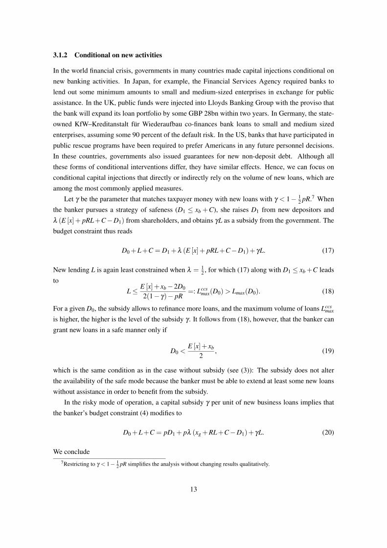
3.1.2 Conditional on new activities
In the world financial crisis, governments in many countries made capital injections conditional on
new banking activities. In Japan, for example, the Financial Services Agency required banks to
lend out some minimum amounts to small and medium-sized enterprises in exchange for public
assistance. In the UK, public funds were injected into Lloyds Banking Group with the proviso that
the bank will expand its loan portfolio by some GBP 28bn within two years. In Germany, the state-
owned KfW–Kreditanstalt fur Wiederaufbau co-finances bank loans to small and medium sized
enterprises, assuming some 90 percent of the default risk. In the US, banks that have participated in
public rescue programs have been required to prefer Americans in any future personnel decisions.
In these countries, governments also issued guarantees for new non-deposit debt. Although all
these forms of conditional interventions differ, they have similar effects. Hence, we can focus on
conditional capital injections that directly or indirectly rely on the volume of new loans, which are
among the most commonly applied measures.
Let γ be the parameter that matches taxpayer money with new loans with γ < 1− 12
pR.7 When
the banker pursues a strategy of safeness (D1 ≤ xb +C), she raises D1 from new depositors and
λ (E [x]+ pRL+C−D1) from shareholders, and obtains γL as a subsidy from the government. The
budget constraint thus reads
D0 +L+C = D1 +λ (E [x]+ pRL+C−D1)+ γL. (17)
New lending L is again least constrained when λ = 12, for which (17) along with D1 ≤ xb +C leads
to
L≤ E [x]+ xb−2D0
2(1− γ)− pR=: Lccs
max(D0) > Lmax(D0). (18)
For a given D0, the subsidy allows to refinance more loans, and the maximum volume of loans Lccsmax
is higher, the higher is the level of the subsidy γ . It follows from (18), however, that the banker can
grant new loans in a safe manner only if
D0 <E [x]+ xb
2, (19)
which is the same condition as in the case without subsidy (see (3)): The subsidy does not alter
the availability of the safe mode because the banker must be able to extend at least some new loans
without assistance in order to benefit from the subsidy.
In the risky mode of operation, a capital subsidy γ per unit of new business loans implies that
the banker’s budget constraint (4) modifies to
D0 +L+C = pD1 + pλ (xg +RL+C−D1)+ γL. (20)
We conclude
7Restricting to γ < 1− 12 pR simplifies the analysis without changing results qualitatively.
13
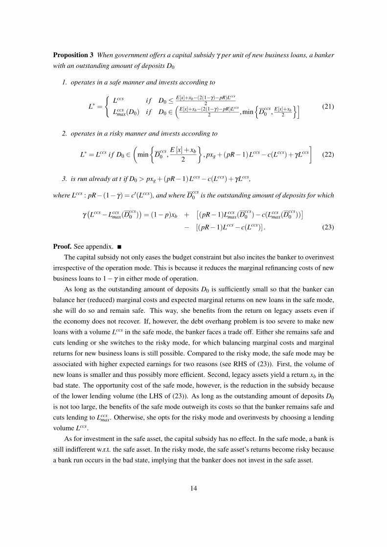
Proposition 3 When government offers a capital subsidy γ per unit of new business loans, a banker
with an outstanding amount of deposits D0
1. operates in a safe manner and invests according to
L∗ =
{Lccs i f D0 ≤ E[x]+xb−(2(1−γ)−pR)Lccs
2
Lccsmax(D0) i f D0 ∈
(E[x]+xb−(2(1−γ)−pR)Lccs
2,min
{Dccs
0 ,E[x]+xb
2
}] (21)
2. operates in a risky manner and invests according to
L∗ = Lccs i f D0 ∈(
min
{Dccs
0 ,E [x]+ xb
2
}, pxg +(pR−1)Lccs− c(Lccs)+ γLccs
](22)
3. is run already at t if D0 > pxg +(pR−1)Lccs− c(Lccs)+ γLccs,
where Lccs : pR− (1−γ) = c′(Lccs), and where Dccs0 is the outstanding amount of deposits for which
γ(Lccs−Lccs
max(Dccs0 )
)= (1− p)xb +
[(pR−1)Lccs
max(Dccs0 )− c(Lccs
max(Dccs0 ))
]− [(pR−1)Lccs− c(Lccs)] . (23)
Proof. See appendix.
The capital subsidy not only eases the budget constraint but also incites the banker to overinvest
irrespective of the operation mode. This is because it reduces the marginal refinancing costs of new
business loans to 1− γ in either mode of operation.
As long as the outstanding amount of deposits D0 is sufficiently small so that the banker can
balance her (reduced) marginal costs and expected marginal returns on new loans in the safe mode,
she will do so and remain safe. This way, she benefits from the return on legacy assets even if
the economy does not recover. If, however, the debt overhang problem is too severe to make new
loans with a volume Lccs in the safe mode, the banker faces a trade off. Either she remains safe and
cuts lending or she switches to the risky mode, for which balancing marginal costs and marginal
returns for new business loans is still possible. Compared to the risky mode, the safe mode may be
associated with higher expected earnings for two reasons (see RHS of (23)). First, the volume of
new loans is smaller and thus possibly more efficient. Second, legacy assets yield a return xb in the
bad state. The opportunity cost of the safe mode, however, is the reduction in the subsidy because
of the lower lending volume (the LHS of (23)). As long as the outstanding amount of deposits D0
is not too large, the benefits of the safe mode outweigh its costs so that the banker remains safe and
cuts lending to Lccsmax. Otherwise, she opts for the risky mode and overinvests by choosing a lending
volume Lccs.
As for investment in the safe asset, the capital subsidy has no effect. In the safe mode, a bank is
still indifferent w.r.t. the safe asset. In the risky mode, the safe asset’s returns become risky because
a bank run occurs in the bad state, implying that the banker does not invest in the safe asset.
14
3.2 Deposit guarantees
In fall 2008, governments of many countries responded to the financial crisis also by declaring
blanket guarantees for new debt, in particular deposits. Although coverage differed across countries,
the general aim was to reduce systemic risks due to spillover effects and to prevent a freezing of the
loan markets.
Guarantee schemes tend to reduce the proper incentives for bankers. They lower market disci-
pline, and thus create moral hazard, because depositors no longer have an incentive to control the
risk of a bank (Nier and Baumann, 2006). However, even when deposit guarantees are supplemented
with a proper regulatory supervision which substitutes for market discipline, they still influence the
banker’s attitude toward risk and her ability to grant new loans.
To see this, assume that government ensures that only depositors, who are not repaid by the bank
when a run occurs, but not the banker benefit from the guarantee. Then, guaranteeing new deposits
has no effect on the banker’s behavior when she operates in the safe mode, in which there is no run.
By contrast, when operating in the risky mode, a guarantee serves to fully repay depositors in the
bad state, in which the bank is run. Accordingly, the banker’s budget constraint (4) modifies to
D0 +L+C = D1 + pλ (xg +RL+C−D1) . (24)
The guarantee effectively subsidizes deposits in the risky mode. The banker has to pay only an
expected return p per unit of deposits (1− p is covered by the guarantee) while she would have to
compensate shareholders for their opportunity costs completely. Therefore, the banker capitalizes
the most on the subsidy if she does not issue any equity or non-deposit debt at all, λ = 0. But bank
capital is not only more expensive. It is also useless since opting for the risky mode implies that
capital is too small to prevent a run in the bad state. Accordingly, bank capital is strictly dominated
by deposits. The banker’s budget constraint in the risky mode (24) changes to
D1 = D0 +L+C. (25)
This leads us to
Proposition 4 When government offers a deposit guarantee, a banker with an outstanding amount
of deposits D0
1. operates in a safe manner and invests according to
L∗ = L f b i f D0 ≤ Ddg0 <
E [x]+ xb− (2− pR)L f b
2(26)
2. operates in a risky manner and invests according to
L∗ = Ldg i f D0 ∈(
Ddg0 ,
pxg +(pR− p)Ldg− c(Ldg)p
](27)
15
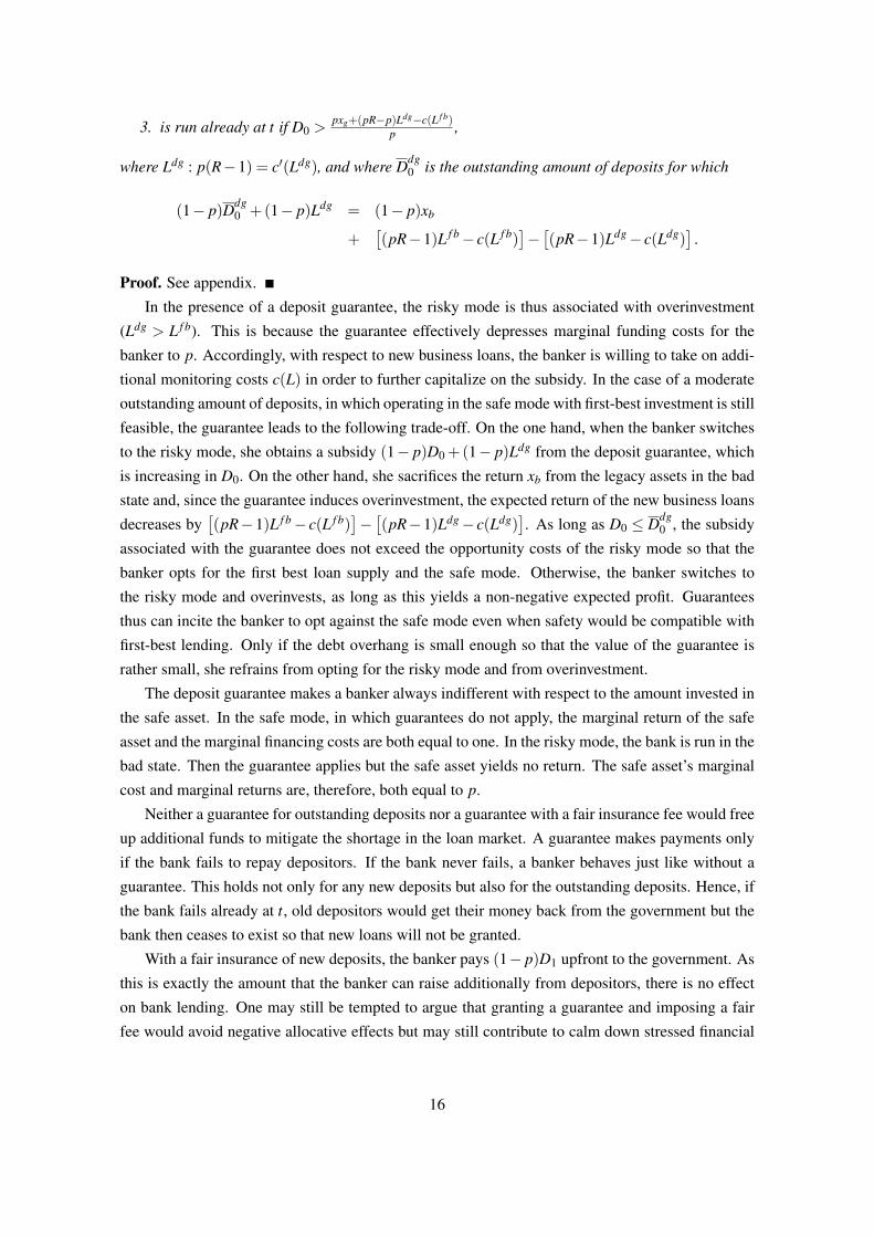
3. is run already at t if D0 >pxg+(pR−p)Ldg−c(L f b)
p ,
where Ldg : p(R−1) = c′(Ldg), and where Ddg0 is the outstanding amount of deposits for which
(1− p)Ddg0 +(1− p)Ldg = (1− p)xb
+[(pR−1)L f b− c(L f b)
]− [(pR−1)Ldg− c(Ldg)
].
Proof. See appendix.
In the presence of a deposit guarantee, the risky mode is thus associated with overinvestment
(Ldg > L f b). This is because the guarantee effectively depresses marginal funding costs for the
banker to p. Accordingly, with respect to new business loans, the banker is willing to take on addi-
tional monitoring costs c(L) in order to further capitalize on the subsidy. In the case of a moderate
outstanding amount of deposits, in which operating in the safe mode with first-best investment is still
feasible, the guarantee leads to the following trade-off. On the one hand, when the banker switches
to the risky mode, she obtains a subsidy (1− p)D0 +(1− p)Ldg from the deposit guarantee, which
is increasing in D0. On the other hand, she sacrifices the return xb from the legacy assets in the bad
state and, since the guarantee induces overinvestment, the expected return of the new business loans
decreases by[(pR−1)L f b− c(L f b)
]− [(pR−1)Ldg− c(Ldg)
]. As long as D0 ≤ Ddg
0 , the subsidy
associated with the guarantee does not exceed the opportunity costs of the risky mode so that the
banker opts for the first best loan supply and the safe mode. Otherwise, the banker switches to
the risky mode and overinvests, as long as this yields a non-negative expected profit. Guarantees
thus can incite the banker to opt against the safe mode even when safety would be compatible with
first-best lending. Only if the debt overhang is small enough so that the value of the guarantee is
rather small, she refrains from opting for the risky mode and from overinvestment.
The deposit guarantee makes a banker always indifferent with respect to the amount invested in
the safe asset. In the safe mode, in which guarantees do not apply, the marginal return of the safe
asset and the marginal financing costs are both equal to one. In the risky mode, the bank is run in the
bad state. Then the guarantee applies but the safe asset yields no return. The safe asset’s marginal
cost and marginal returns are, therefore, both equal to p.
Neither a guarantee for outstanding deposits nor a guarantee with a fair insurance fee would free
up additional funds to mitigate the shortage in the loan market. A guarantee makes payments only
if the bank fails to repay depositors. If the bank never fails, a banker behaves just like without a
guarantee. This holds not only for any new deposits but also for the outstanding deposits. Hence, if
the bank fails already at t, old depositors would get their money back from the government but the
bank then ceases to exist so that new loans will not be granted.
With a fair insurance of new deposits, the banker pays (1− p)D1 upfront to the government. As
this is exactly the amount that the banker can raise additionally from depositors, there is no effect
on bank lending. One may still be tempted to argue that granting a guarantee and imposing a fair
fee would avoid negative allocative effects but may still contribute to calm down stressed financial
16
markets. However, since the model here takes the effects of looming bank runs already into account,
this argument loses much of its bite.
3.3 Bad bank
In response to banking crises, several countries encouraged banks to establish so called bad banks.
This has been also the case in the recent crisis. The general aim of bad banks is to rescue distressed
financial institutions by relieving them of legacy assets in order to foster new lending. While the
design of bad banks varies across countries, all concepts have one major principle in common.
When a financial institution opts to establish a bad bank, it substitutes its legacy assets, which are
characterized by a high degree of risk and a low expected value, for a payment stream, which is less
risky.
To translate the concept of a bad bank into our model, suppose that the bank can replace its risky
legacy assets by a certain quantity y of the safe asset. That is, we assume that when participating in a
bad bank, the banker can get rid of her existing risks completely and faces only the risks associated
with new loans. In this case, the volume of new deposits is restricted by D1≤ y+C in the safe mode,
with C being the quantity of the safe asset acquired in addition to what the banker gets in exchange
for legacy assets. Accordingly, if y > xb the bad bank allows the banker to issue more deposits
without having to switch to the risky mode. After replacing legacy assets, the budget constraint of
the banker in the safe mode is
D0 +L+C = D1 +λ (y+ pRL+C−D1) , (28)
and the maximum volume of new loans in the safe mode is
L≤ 2(y−D0)2− pR
=: Lbbmax(D0), (29)
implying that the banker can operate safely if
D0 ≤ y. (30)
Compared to the case without government interventions (see (2) and (3)), the existence of a bad
bank thus improves the banker’s ability to extend loans safely if the funding liquidity of her assets
improves, i. e. if y > E[x]+xb2
. Hence, although the quantity y of the safe asset obtained by the swap
may be smaller than the expected value of the legacy assets, the bank can extend more new loans in
the safe mode as long as y is not too small. The reason is that due to the swap of assets, the banker
can issue deposits against the complete expected value y of the safe asset. Therefore, in contrast to
keeping the legacy assets on the balance sheet, the banker relies less on equity issues, which is an
inefficient financing instrument as the banker can extract rents from the shareholders.
If y > E[x]+xb2
is not met, the banker has no incentive to take part in a bad bank program. This
result indicates that a bad bank can be a useful instrument. By lowering the risk of the bank’s future
17
earnings, it allows for a stronger commitment of the banker vis-a-vis her financiers through the use
of deposits and thus eventually improves her ability to obtain funding for new businesses.
With a bad bank, the banker can also operate in the risky mode by issuing deposits with face
value D1 ∈ (y+C,y+RL+C], so that depositors are repaid only if the economy recovers. Accord-
ingly, the banker’s budget constraint in the risky mode reads
D0 +L+C = pD1 + pλ (y+RL+C−D1) . (31)
We conclude
Proposition 5 When a banker with an outstanding amount of deposits D0 has participated in a bad
bank, she
1. operates in a safe manner and invests according to
L∗ =
⎧⎨⎩ L f b i f D0 ≤ 2y−(2−pR)L f b
2
Lbbmax(D0) i f D0 ∈
(2y−(2−pR)L f b
2,min
{D0,y
}] (32)
2. operates in a risky manner and invests according to
L∗ = L f b i f D0 ∈(
min{
Dbb0 ,y
}, py+(pR−1)L f b− c(L f b)
](33)
3. is run already at t if D0 > py+(pR−1)L f b− c(L f b),
where Dbb0 is the outstanding amount of deposits for which
[(pR−1)L f b− c(L f b)
]−[(pR−1)Lbb
max(Dbb0 )− c(Lbb
max(Dbb0 ))
]= (1− p)y. (34)
Proof. See appendix.
The proposition shows that a bad bank does not alter the banker’s incentives to provide new
loans. This is not surprising. A bad bank concept is backward looking in the sense that it only
affects the existing balance sheet. It thus does not influence new businesses of the bank so that
it does not affect the marginal costs and benefits of new loans. Therefore, a bad bank has similar
implications as a lump sum transfer.
4 Discussion
4.1 An assessment of policy measures
Our assessment of policy measures follows a two-stage selection process. In a first stage, a policy
measure qualifies if it 1) avoids a default on systemically important bank liabilities, 2) fosters new
business lending without inciting banks to overinvest, and 3) does not encourage further excessive
18
risk taking. In the second stage, when two or more measures sort out these problems equally well,
the one should be preferred which is associated with the smallest expected fiscal burden because a
measure that involves less taxpayer money implies less distortions due to taxation.
Starting with deposit guarantees, we have seen that they primarily incite banks to choose a
fragile capital structure and to overinvest in risky assets, a potentially dangerous combination which
may prepare the ground for the next bubble and subsequent crisis. Therefore, guarantees fulfill
neither function 2) nor 3).
As for conditional capital injections, we have seen that subsidizing new lending is associated
with unintended effects. Like deposit guarantees, the subsidy induces banks operating in the risky
mode to overinvest. However, even those banks that would remain safe and provide new business
loans according to the first best without a subsidy, are incited to overinvest. Hence, subsidizing new
business loans is efficiency-enhancing only for banks with an intermediate debt overhang, which still
prefer to operate safely but are unable to grant more new loans than associated with the first best.
For them, the subsidy may be helpful because it eases the financial constraint without giving scope
for overinvestment. Altogether, conditional capital injections do not fulfill function 2) properly.
Like subsidies conditional on new activities, a government assistance that does not depend on
new businesses of the banker also releases banks from their debt burden, thereby expanding the
capacity of banks to provide new loans in a safe manner. Unlike subsidies conditional on new
activities, however, they do not incite a bank to overinvest. A bad bank, which allows banks to
swap risky legacy assets for a certain quantity of the safe asset, is also suitable to implement the
same allocation as unconditional capital injections. We conclude that only unconditional capital
injections and the bad bank qualify as effective policy measures.
Notwithstanding their merits, unconditional capital injections and the bad bank are by no means
perfect when taking their fiscal effects for taxpayer into account. As long as the government is
unable to discriminate between those banks who are really in need of support and those who are
not, government assistance will imply a waste of taxpayers money. Consider the lump sum transfer.
There, banks with a small debt overhang do not need support but will also draw on this kind of
assistance and invest into the safe asset. Banks with a severe debt overhang will not change their
behavior at all. They would grant loans according to the first-best anyway but still in a risky manner
when the lump sum is too small to provide them with the proper incentives to switch into the safe
mode. For these banks, taxpayer money is again wasted. Finally, for banks with a moderate debt
overhang public funds would not be wasted, but banks may be granted too little support to remove
their refinancing restrictions so that they still underinvest.
To address this selection problem, government could make its support conditional on the existing
debt burden D0 because banks with a relatively small level of outstanding deposits shall be likely to
invest efficiently and safely without support from the government. This, however, is not necessarily
true. The extent of investment inefficiency does not only depend on the size of the pre-existing
debt but also on the first-best loan supply L f b (which is unknown to the government). That is, it
may be that banks with a relatively small debt burden will invest rather inefficiently due to a large
19
L f b while other banks with a large D0 are able and willing to provide first best lending in a safe
manner. It is also not advisable to prevent banks from investing in the safe asset. In the safe mode,
banks are always indifferent with respect to the safe asset, irrespective whether they underinvest
in new loans or not. Hence, investment in safe assets is not a good indicator for the strength of
the debt overhang problem ex ante. Moreover, conditioning on investment in the safe asset makes
the financial assistance again dependent on new banking activities ex post and thus incites banks to
overinvest in new loans.
Compared to a lump sum subsidy, funding a bad bank is even less cost efficient. In order to have
a bank granting new loans of some L in a safe manner, the government has to inject(1− 1
2pR
)L +
D0− 12(E[x]+ xb) as lump sum, whereas taxpayers have to pay
(1− 1
2pR
)L + D0−X in the case
of a bad bank, with X being the expected value of legacy assets to taxpayers. As the specific skills
of the banker are needed to extract the full value of these assets, we have X < 12(E[x]+ xb). Hence,
although a bad bank does not induce any disincentives with respect to new loans, a lump sum
subsidy has the same effect at a lower fiscal cost. The comparative disadvantage of bad banks thus
mainly stems from the loss in the bankers’ specific expertise in collecting loans.8
4.2 Government subsidy versus financial investment
A further feature of our analysis is that banks should not be obliged to pay the government a market
return on its financial stake. Either this kind of aid will not be accepted, or government funds just
crowd out private funds. Accordingly, government is not advised to require, e.g., fair insurance
premiums for granting deposit guarantees amid a banking crisis. This claim has to be qualified,
though. It does not mean that government help should always be free of charge. A proper pricing
of the safety net is indeed an important lesson learned from the recent crisis. This pricing should,
first and foremost, mitigate adverse incentives that arise from the provision of the safety net, but not
primarily reduce taxpayers money at risk. It is, however, unlikely that properly priced prevention
measures will completely rule out the emergence of a crisis. Once the banking system suffers from
a debt overhang, it is too late for charging a price as bankers have only little scope to influence the
value of legacy assets and of debt that had been issued in the past.9
4.3 Further proposals
It has also been proposed that the government should subsidize equity or deposit issues. This might
be rational, so the argument goes, because banks which are able to raise more funds on the market
are often supposed to be more valuable. If there is still a shortage in loan supply, these banks are
8A bad bank is also less cost efficient than a conditional capital injection. For the latter to induce a banker to grant
L in a safe manner, γ should equal(1− 1
2pR)L+D0− 1
2(E[x]+xb)
Limplying a capital injection of the same magnitude as in the
case of a lump sum transfer.9This may explain why government interventions have sometimes been disappointing. For example, Bank of America
announced in December 2009 that it would be about to repay 45bn dollars in TARP funds. In the 12 month since the
government first made its investment in the bank, the US government earned about 3.6bn dollars for its one-year stake in
Bank of America. Within this time period, the bank originated a total of only 760m dollars in new loans.
20
considered worthy of being supported.10 Such a subsidy, however, is just another type of capital in-
jections conditional on new banking businesses. Although it does not refer to new lending activities,
a banker can influence the amount of the subsidy by adapting equity and deposit issues. By reducing
effective marginal refinancing costs, the subsidy distorts the banker’s investment incentives and in-
duces her to overinvest irrespective of the operation mode. While this disadvantage applies to both
forms of subsidies, subsidizing new deposits has a further disadvantage. Like deposit guarantees, it
makes deposit financing more attractive relative to equity financing so that the banker has a stronger
tendency to opt for the risky mode of operation, in which she issues a higher volume of deposits.
Hart and Zingales (2009) proposed that large financial intermediaries should be subject to reg-
ulatory margin calls. Whenever an intermediary becomes risky (in the sense that the probability of
default on its debt exceeds some pre-specified threshold), shareholders shall inject fresh funds in or-
der to make debt safe. Imposing such a margin call prevents a bank from operating in a risky mode,
but is associated with underinvestment and some banks dropping out of the market. Although this
measure cannot deal with the problem of shortages in the loan market, it may reasonably supplement
other interventions, in particular conditional capital injections, in order to reduce the associated in-
centives to pursue a risky business model. The drawback then is that CDS spreads may decrease
just because of expected government interventions.
5 Summary
In this paper, we have evaluated policy measures that aim at stopping the fall in bank loan supply
following a banking crisis. We have presented a dynamic banking model in which a debt overhang
induces banks either to curtail lending or to choose a fragile capital structure. Different government
interventions influence banks’ lending behavior, capital structure and risk taking in different ways.
Measures can be grouped into two categories. One group comprises measures that cope with the
existing debt. Measures that deal with the adverse effects of the debt overhang from the second
group. When government grants assistance in order to mitigate the adverse effects of the debt
overhang by supporting new lending or the issue of new debt and equity, banks can influence the
scale of the assistance by changing new contracts. Since banks can externalize risks then, there will
be excessive risk taking and overinvestment which put the future stability of the banking system
at risk. Providing unconditional financial assistance to banks is a better solution as it does not
incite banks to have a fragile capital structure risk or to overinvest in risky loans. In the end, this
solution recognizes that the debt overhang is the result of past lending behavior and capital structure
decisions of banks.
10For example, Calomiris (2008) proposed that government should inject preferred stocks into banks in order to recap-
italize them. In particular, being matched by common stock issues underwritten by private investors, it would recapitalize
banks in “an incentive compatible manner to facilitate banks’ abilities to maintain and grow assets.”
21
Appendix
Proof of Proposition 1
1. Suppose the banker has opted for the safe mode. Solving (1) for D1 and substitution in (5)
yields
maxL,C,λ [E [x]+ (pR−1)L−D0− c(L)] =: Γ(L)
s.t. L ∈[
λE[x]−(1−λ )C−D0
1−λ pR ,λE[x]+(1−λ )xb−D0
1−λ pR
], λ ∈ [
0, 12
], and L,C ≥ 0.
(35)
Note that Γ is independent of λ and C. Moreover, the upper bound of L is increasing in
λ while the lower bound of L is decreasing in C for all C ≤ λE[x]−D0
1−λ . Therefore, we can
conclude that λ = 12
and C = max{E[x]−2D0,0} is among the set of optimal decisions of
the banker, so that (35) simplifies to
maxL Γ(L) = [E [x]+ (pR−1)L−D0− c(L)] s.t. L ∈[0,
E[x]+xb−2D0
2−pR
].
As ∂Γ∂L = (pR−1)− c′(L) is decreasing in L and equal to zero for L = L f b, the optimal loan
volume is L∗S = min{
L f b,Lmax(D0)}
. The safe mode is feasible if L∗S ≥ 0, implying D0 ≤E[x]+xb
2. Then, the banker’s expected payoff is
Γ(L∗S) = E [x]+ (pR−1)min{
L f b,Lmax(D0)}−D0− c
(min
{L f b,Lmax(D0)
}). (36)
2. Suppose the banker has opted for the risky mode. Solving (4) for D1 and substitution in (6)
We neglect D1 ∈ (xb +C,xg + RL +C] but show that it will be met in equilibrium. As Ωis independent from λ and decreasing in C, λ = 0 and C = 0 is among the set of optimal
decisions of the banker, so that (37) simplifies to
maxL Ω(L) = [pxg +(pR−1)L−D0− c(L)] s.t. L≥ 0.
As ∂Ω∂L = (pR−1)− c′(L) is decreasing in L and equal to zero for L = L f b, the optimal loan
volume is L∗R = L f b. Then, the banker’s expected payoff is
Ω(L∗R) = pxg +(pR−1)L f b−D0− c(L f b) . (38)
3. Comparing Γ(L∗S) and Ω(L∗R) yields
(a) If D0 ≤ E[x]+xb−(2−pR)L f b
2and thus L∗S = L f b, it follows from (36) and (38) that Γ(L∗S) >
Ω(L∗R): the banker operates in a safe manner and invests according to L f b.
22
(b) If D0 ∈(
E[x]+xb−(2−pR)L f b
2,
E[x]+xb2
]and thus L∗S = Lmax(D0), it follows from (36) and
(38) that Γ(L∗S)≥Ω(L∗R) only if
(1− p)xb ≥[(pR−1)L f b− c(L f b)
]− [(pR−1)Lmax(D0)− c(Lmax(D0))] . (39)
The RHS of (39) is increasing in D0. Therefore, the banker
• operates in a safe manner and invests according to Lmax(D0) if D0 ∈(E[x]+xb−(2−pR)L f b
2,min
{D0,
E[x]+xb2
}],
• operates in a risky manner and invests according to L f b if D0 ∈(
D0,E[x]+xb
2
].
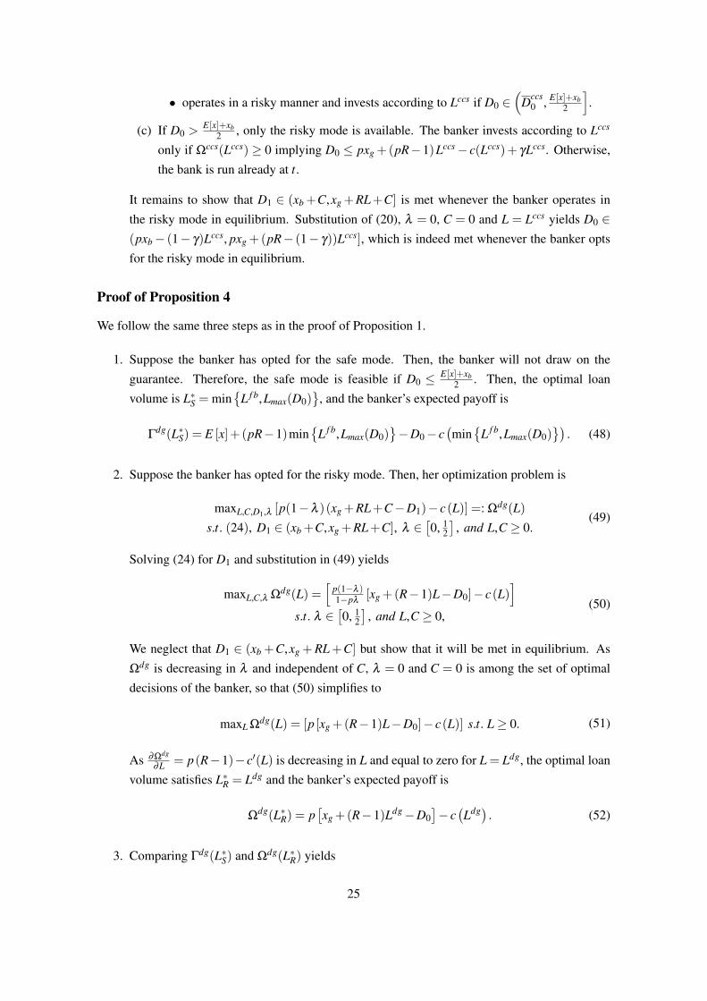
(c) If D0 > E[x]+xb2
, only the risky mode is available. The banker invests according to L f b
only if Ω(L f b)≥ 0 implying D0 ≤ pxg +(pR−1)L f b− c(L f b). Otherwise, the bank is
run already at t.
It remains to show that D1 ∈ (xb +C,xg +RL+C] is met whenever the banker operates in
the risky mode in equilibrium. Substitution of (4), λ = 0, C = 0 and L = L f b yields D0 ∈(pxb−L f b, pxg +(pR− 1)L f b], which is indeed met whenever the banker opts for the risky
mode in equilibrium.
Proof of Proposition 2
The proof is essentially equivalent to the proof of Proposition 1 with an outstanding amount of
deposits of D0−S instead of D0.
Proof of Proposition 3
We follow the same three steps as in the proof of Proposition 1.
1. Suppose the banker has opted for the safe mode. Her optimization problem is
2and thus L∗S = Lccs, it follows from (43) and (46) that
Γccs(L∗S) > Ωccs(L∗R) so that the banker operates in a safe manner and invests according
to Lccs.
(b) If D0 ∈(
E[x]+xb−(2(1−γ)−pR)Lccs
2,
E[x]+xb2
]and thus L∗S = Lccs
max(D0), it follows from (43)
and (46) that Γccs(L∗S)≥Ωccs(L∗R) only if
(1− p)xb − [(pR− (1− γ))Lccs− c(Lccs)] (47)
≥ − [(pR− (1− γ))Lccsmax(D
ccs0 )− c(Lccs
max(Dccs0 ))]
The RHS of (47) is decreasing in L for all L≤ Lccs. Therefore, the banker
• operates in a safe manner and invests according to Lccsmax(D0) if D0 ∈(
E[x]+xb−(2(1−γ)−pR)Lccs
2,min
{Dccs
0 ,E[x]+xb
2
}],
24
• operates in a risky manner and invests according to Lccs if D0 ∈(
Dccs0 ,
E[x]+xb2
].
(c) If D0 > E[x]+xb2
, only the risky mode is available. The banker invests according to Lccs
only if Ωccs(Lccs) ≥ 0 implying D0 ≤ pxg +(pR−1)Lccs− c(Lccs)+ γLccs. Otherwise,
the bank is run already at t.
It remains to show that D1 ∈ (xb +C,xg +RL+C] is met whenever the banker operates in
the risky mode in equilibrium. Substitution of (20), λ = 0, C = 0 and L = Lccs yields D0 ∈(pxb− (1− γ)Lccs, pxg +(pR− (1− γ))Lccs], which is indeed met whenever the banker opts
for the risky mode in equilibrium.
Proof of Proposition 4
We follow the same three steps as in the proof of Proposition 1.
1. Suppose the banker has opted for the safe mode. Then, the banker will not draw on the
guarantee. Therefore, the safe mode is feasible if D0 ≤ E[x]+xb2
. Then, the optimal loan
volume is L∗S = min{
L f b,Lmax(D0)}
, and the banker’s expected payoff is
Γdg(L∗S) = E [x]+ (pR−1)min{
L f b,Lmax(D0)}−D0− c
(min
{L f b,Lmax(D0)
}). (48)
2. Suppose the banker has opted for the risky mode. Then, her optimization problem is
∂L = p(R−1)−c′(L) is decreasing in L and equal to zero for L = Ldg, the optimal loan
volume satisfies L∗R = Ldg and the banker’s expected payoff is
Ωdg(L∗R) = p[xg +(R−1)Ldg−D0
]− c(Ldg) . (52)
3. Comparing Γdg(L∗S) and Ωdg(L∗R) yields
25
(a) If D0≤ E[x]+xb−(2−pR)L f b
2and thus L∗S = L f b, it follows from (48) and (52) that Γdg(L∗S)≥
Ωdg(L∗R) only if
(1− p)xb +[(pR−1)L f b− c(L f b)
]− [(pR−1)Ldg− c(Ldg)
](53)
≥ (1− p)Ddg0 +(1− p)Ldg.
The RHS of (53) is increasing in D0. Therefore, the banker
• operates in a safe manner and invests according to L f b if D0 ≤ Ddg0 ,
• operates in a risky manner and invests according to Ldg if D0 ∈(Ddg
0 ,E[x]+xb−(2−pR)L f b
2
].
(b) If D0 ∈(
E[x]+xb−(2−pR)L f b
2,
E[x]+xb2
]and thus L∗S = Lmax(D0), the banker will operate in
a risky manner and invest according to Ldg. To see this, note first that Γdg(Lmax(D0)) <
Γdg(L f b) and Ωdg(L f b) < Ωdg(Ldg), since otherwise, the banker would choose L f b
instead of Ldg in the risky mode. Accordingly, it remains to show that Γdg(L f b) <
Ωdg(L f b), which is true if D0 > xb−L f b, which is true in the case considered here.
(c) If D0 > E[x]+xb2
, only the risky mode is available. The banker operates in this risky mode
and invests according to Ldg only if Ωdg(Ldg) ≥ 0 implying D0 ≤ pxg+(pR−p)Ldg−c(Ldg)p .
Otherwise, the bank is run already at t.
It remains to show that D1 ∈ (xb +C,xg +RL+C] is met whenever the banker operates in
the risky mode in equilibrium. Substitution of (24), λ = 0, C = 0 and L = Ldg yields D0 ∈(xb−Ldg,xg +(R−1)Ldg], which is indeed met whenever the banker opts for the risky mode
in equilibrium.
Proof of Proposition 5
The proof is essentially equivalent to the proof of Proposition 1 with xb = E[x] = y.
References
Acharya V V (2009) A theory of systemic risk and design of prudential bank regulation. J Financ
Stab 5:224–255.
Aghion P, Bolton P, Fries S (1999) Optimal design of bank bailouts: The case of transition
economies. J Inst Theor Econ 155:51–70.
Allen F, Gale D (2000) Financial contagion. J Polit Econ 108:1–33.
Calomiris CW (2008) A matched preferred stock plan for government assistance.
http://www.voxeu.org/index.php?q=node/1683.
26
Dell’Ariccia G, Detragiache E, Rajan R(2008) The real effects of banking crises. J Financ Interme-
diation 17:89–112.
Demirguc-Kunt A, Detragiache E (2002) Does deposit insurance increase banking systemstability?
An empirical investigation. J Monetary Econ 49:1373–1406.
Diamond DW (2001) Should banks be recapitalized? Fed Reserve Bank of Richmond Econ Quart
87:71–96.
Diamond DW, Rajan R (2000) A theory of bank capital. J Financ 55:2431–2465.
Diamond DW, Rajan R (2001) Liquidity risk, liquidity creation, and financial fragility: A theory of
banking. J Polit Econ 109:287–327.
Diamond DW, Rajan R (2005) Liquidity shortages and banking crisis. J Financ 60:615–647.
Flannery MJ (2009) Stabilizing large financial institutions with contingent capital Certificates (Oc-
tober 6, 2009). Available at http://ssrn.com/abstract=1485689
Freixas X, Giannini C, Hoggarth G, Soussa F (2000) Lender of last resort: what have we learned
since Bagehot? J Financ Serv Res 18:63–84.
Hart O, Zingales L (2009) A new capital regulation for large financial institutions. Discussion Paper
7298, Centre for Economic Policy Research CEPR, London.
Holmstrom B, Tirole J (1997) Financial intermediation, loanable funds, and the real sector. Quart J
Econ 112:663–691.
Laeven L, Valencia F (2008) Systemic banking crises: A new database. Working Paper WP/08/224,
International Monetary Fund, Washington.
Mitchell J (2001) Bad debts and the cleaning of banks’ balance sheets: An application to transition
Nier E, Baumann U (2006) Market discipline, disclosure and moral hazard in banking. J Financ
Intermediation 3:332–361.
Panageas S (2010) Bailouts, the incentive to manage risk, and financial crises. J Financ Econ
95:296–311.
Panetta F, Faeh T, Grande G, Ho C, King M, Levy A, Signoretti FM, Taboga M, Zaghini A (2009) An
assessment of financial sector rescue programmes. Questioni di Economia e Finanza (Occasional
Paper) 47, Banca d’Italia, Rome.
27
Philippon T, Schnabl P (2009) Efficient recapitalization. Discussion Paper 7516, Centre for Eco-
nomic Policy Research CEPR, London.
Peek J, Rosengren E (1995) The capital crunch: Neither a borrower nor a lender be. J Money Credit
Bank 27:625–638.
Praet P, Nguyen G (2008) Overview of recent policy initiatives in response to the crisis. J Financ
Stability 4:368–375.
28
Die folgenden Diskussionspapiere wurden seit Juni 2008 veröffentlicht:
The following Discussion Papers have been published since June 2008:
1 2008 Finanzierungsentscheidungen mittelständischer Christoph Börner Unternehmer – Eine empirische Analyse des Dietmar Grichnik Pecking-Order-Modells Franz Reize
Solvig Räthke
2 2008 Credit Default Swaps and the Stability of the Frank Heyde Banking Sector Ulrike Neyer
3 2008 Are Rating Splits a Useful Indicator for the Opacity Achim Hauck of an Industry? Ulrike Neyer
4 2008 Gewährträgerhaftung im öffentlich-rechtlichen Uwe Vollmer Bankensektor: Konsequenzen für die Unterneh- Achim Hauck mensfinanzierung
1 2009 Wirtschaftliche Wirkungen der Freistellung Guido Förster ausländischer Betriebsstätteneinkünfte unter Progressionsvorbehalt
2 2009 Exchange Traded Funds in Deutschland: Andreas Wiesner simply buying the Index? Heinz-Dieter Smeets
3 2009 A Lender of Last Resort for Public Banks? Achim Hauck Theory and an Application to Japan Post Bank Uwe Vollmer
4 2009 Dynamik der Staatsverschuldung Heinz-Dieter Smeets
5 2009 Finanzkrise: Ursachen, Wirkungen und Heinz-Dieter Smeets (wirtschafts-)politische Reaktionen
1 2010 Optimierung der Tarifvergünstigungen für Dirk Schmidtmann außerordentliche Einkünfte und des negativen Progressionsvorbehalts durch die Schedulenbesteuerung gem. § 34a EStG und §§ 32d, 43 Abs. 5 EStG
2 2010 The Euro Area Interbank Market and the Liquidity Achim Hauck Management of the Eurosystem in the Financial Crisis Ulrike Neyer
3 2010 Government Interventions in Banking Crises: Diemo Dietrich Assessing Alternative Schemes in a Banking Model Achim Hauck of Debt Overhang