Munich Personal RePEc Archive New Evidence on Gibrat’s Law for Cities Rafael Gonz´ alez-Val and Luis Lanaspa and Fernando Sanz 5. September 2008 Online at http://mpra.ub.uni-muenchen.de/10411/ MPRA Paper No. 10411, posted 11. September 2008 04:58 UTC
Transcript
MPRAMunich Personal RePEc Archive
New Evidence on Gibrat’s Law for Cities
Rafael Gonzalez-Val and Luis Lanaspa and Fernando Sanz
5. September 2008
Online at http://mpra.ub.uni-muenchen.de/10411/MPRA Paper No. 10411, posted 11. September 2008 04:58 UTC
1. Introduction The relationship between the growth rate of a quantifiable phenomenon and
initial size is a question with a long history in statistics: do larger entities grow more quickly, or the other way around? On the other hand, perhaps no relationship exists and the rate is independent of size. A fundamental contribution to this debate is that of Robert Gibrat [1931], who observed that the distribution of size (measured by sales or the number of employees) of firms could be approximated well with a lognormal, and that the explanation lay in the growth process of firms tending to be multiplicative and independent of their size. This proposition became known as Gibrat’s Law and was the beginning of a deluge of work exploring the validity of this law for the distribution of firms (see the surveys of John Sutton [1997] and Enrico Santarelli, Luuk Klomp and Roy Thurik [2006]). Gibrat’s Law establishes that no regular behavior of any kind can be deduced between growth rate and initial size.
The fulfilment of this empirical proposition also has consequences on the distribution which follows the variable; in the words of Gibrat [1931] himself “the law of proportionate effect will therefore imply that the logarithms of the variable will be distributed following the [normal distribution]”. Some years later Michael Kalecki [1945], in a classic article, tested this statistical relationship between lognormality and proportional growth under certain conditions, consolidating the conceptual binomial Gibrat’s Law – lognormal distribution.
In the field of urban economics, Gibrat’s Law, especially since the 1990s, has given rise to numerous empirical studies contrasting its validity for city size distributions, arriving at a consensus, not absolute but of a majority, that it holds in the long term. Gibrat’s Law presents the added advantage that as well as explaining relatively well the growth of cities, it can be related to another empirical regularity well known in urban economics, Zipf’s Law, which appears when the so-called Pareto distribution exponent is equal to the unit1. The term was coined after a work by George Zipf [1949], which observed that the frequency of the words of any language is clearly defined in statistical terms by constant values. This has given rise to theoretical works explaining the fulfilment of Gibrat’s Law in the context of external urban local effects and productive shocks, relating them with Zipf’s Law and associating them directly to an equilibrium situation. These theoretical works include Xavier Gabaix [1999], Gilles Duranton [2006, 2007] and Juan C. Córdoba [2008].
Returning to the empirical side, there is an apparent contradiction in these studies, as they normally accept the fulfilment of Gibrat’s Law but at the same time affirm that the distribution followed by city size is a Pareto distribution, very different to the lognormal. Recently, Jan Eeckhout [2004] was able to reconcile both results, by demonstrating (as Jhon B. Parr and Keisuke Suzuki [1973] affirm in a pioneering work) that if size restrictions are imposed on the cities, taking only the upper tail, this skews the analysis. Thus, if all cities are taken, it can be found that the true distribution is lognormal, and that the growth of these cities is independent of size. However, to date, Eeckhout [2004] is the only study to consider the entire city size distribution. But this is
1 If city size distribution follows a Pareto distribution the following expression can be deduced: lnr=a-blnS, where r is rank (1 for the biggest city, 2 for the second biggest and so on), S is the size or population and a and b are parameters, this latter being known as the Pareto exponent. Zipf’s Law is fulfilled when b equals the unit.
2
a short term analysis2, when the phenomenon under study (Gibrat’s Law) is, by definition, a long term result.
The aim of this work is to test empirically the validity of Gibrat’s Law in the growth of cities, using data for all the twentieth century of the complete distribution of cities (without any size restrictions or with no truncation point) in three countries: the US, Spain and Italy. The following section offers a brief overview of the literature on Gibrat’s Law and cities, mainly focusing on the sample sizes used in other studies, and the results obtained. Section 3 presents the databases, with special attention to the US census. From the results we deduce that when we consider the complete distribution of cities (section 4), a tendency to divergence is seen. However, the empirical evidence (section 5.1) shows that this does not impede city size distribution being adequately approximated as a lognormal distribution. In section 5.2 we will try to resolve this apparent contradiction within the theoretical framework developed by Kalecki [1945], proposing a minor modification of his model. Finally, we will relativise the results obtained in this study (and all the earlier ones) showing that the conclusions obtained on the fulfilment or otherwise of Gibrat’s Law depend, first, on sample size (section 6), and second, on city size (section 7). The work ends with our conclusions.
2. Gibrat’s Law for cities. An overview of the literature Following Xavier Gabaix and Yannis M. Ioannides [2004], Gibrat’s law states
that the growth rate of an economic entity (firm, mutual fund, city) of size has a distribution function with mean and variance that are independent of . Therefore, if
is the size of city at the time and is its growth rate, then . Taking logarithms and adding that the rate depends on the initial size, we can obtain the following general expression of the growth equation
S
− 11
SSititS i t g ( )gSit +=
3:
itititit uSSS ++=− −− 11 lnlnln βμ , (1)
where ( g+= 1ln )μ and is a random variable representing the random shocks which the growth rate may suffer, which we shall suppose to be identically and independently distributed for all cities, with
itu
( ) 0=ituE and ( ) 2σ=ituVar ti,∀ . If 0=β Gibrat’s Law holds and we obtain that growth is independent of the initial size.
In this case, ( 0=β ), it is easy to prove that the expected value of the size of city at the time depends only on the number of periods which have passed and on size in
the first period: i t
( ) 0lnln iit StSE +⋅= μ , (2)
while the variance would be given by:
2 Eeckhout [2004] takes data from the United States census of 1990 and 2000, possibly because they are the only ones to be available on line. Moshe Levy (2008) in a comment to Eeckhout (2004) and Jan Eeckhout (2008) in the reply also consider no truncation point, but only for the 2000 US Census data. 3 The size of a city can be defined, according to the literature, in three ways: in levels ( ), in relative
values (
itS
t
itS
S , tS is the mean size) or in shares ( ∑i
it
itS
S ). The crucial parameter in (1) is β , which
determines whether Gibrat’s Law holds. The specification (1) in logs makes the estimation of β robust to the three different definitions of city size.
3
( ) 2ln σ⋅= tSVar it . (3)
Consequently, the mean grows over time, which seems reasonable for many economic variables, but variance does too, which is more debatable.
Remember that if 0=β city growth is proportional, as it does not depend on initial size. Thus, if the estimation of β is significantly different to zero we will reject the fulfilment of Gibrat’s Law. In the case of being greater than zero, we will have divergent growth, because city growth would depend directly and positively on initial size. A sustained process of divergent growth of this kind would result in an increasingly asymmetrical distribution, with small cities getting further and further away from large ones. And if β is negative urban growth would be convergent (mean reversion), as the growth-size ratio would be negative; a larger initial population would mean less growth and vice versa, so that in the long term distribution would tend to be concentrated around a median value. It is simple to prove that when 0≠β expressions (2) and (3) change, becoming
( ) ( ) ( ) 0ln111ln it
t
it SSE ++−+
⋅= ββ
βμ , (4)
( ) ( )ββ
βσ2
11ln 2
22
+−+
⋅=t
itSVar , (5)
and it can be demonstrated (see Appendix) that when and growth is divergent 1>t( 0> )β variance (5) grows even faster than in (3), while if city growth were convergent ( 0< )β variance (5) would be less than in (3).
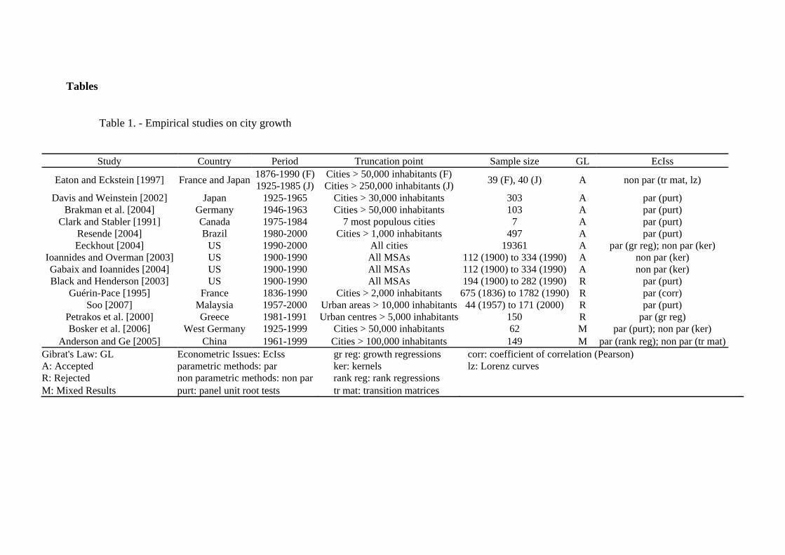
In the 1990s numerous studies began to appear which empirically tested the validity of Gibrat’s Law. Table 1 shows the classification of all the studies on urban economics that we know of. While the countries considered, statistical and econometric techniques used and sample sizes are heterogeneous, the predominating result is the acceptance of Gibrat’s Law.
Thus, both Jonathan Eaton and Zvi Eckstein [1997] and Donald R. Davis and David E. Weinstein [2002] accept its fulfilment for Japanese cities, although they use different sample sections (40 and 303 cities, respectively) and time horizons. Davis and Weinstein [2002] affirm that long-run city size is robust even to large temporary shocks and, in studying the effect of Allied bombing in the Second World War, deduce that the effect of these temporary shocks disappears completely in less than 20 years.
Steven Brakman, Harry Garretsen and Marc Schramm [2004] come to the same conclusion when analysing the impact of bombardment on Germany during the Second World War, concluding that, for the sample of 103 cities examined, bombing had a significant but temporary impact on post-war city growth. Nevertheless, nearly the same authors in Maarten Bosker, Steven Brakman, Harry Garretsen and Marc Schramm [2006] obtain a mixed result with a sample of 62 cities in West Germany: correcting for the impact of WWII Gibrat's Law is found to hold only for about 25% of the sample.
Meanwhile, both J. Stephen Clark and Jack C. Stabler [1991] and Marcelo Resende [2004] also accept the hypothesis of proportional urban growth for Canada and Brazil respectively. The sample size used by Clark and Stabler [1991] is tiny (the 7 most populous Canadian cities), although the main contribution of their work is to
4
propose the use of data panel methodology and unit root tests in the analysis of urban growth. This is also the methodology which Resende [2004] applies to his sample of 497 Brazilian cities.
For the case of the US there are also several works accepting statistically the fulfilment of Gibrat’s Law, whether at the level of cities (Eeckhout [2004] is the first to use all the sample without size restrictions), or with MSAs (Yannis M. Ioannides and Harry G. Overman [2003], whose results reproduce Gabaix and Ioannides, 2004). Also for the US, however, Duncan Black and Vernon Henderson [2003] reject Gibrat’s Law for any sample section, although their database of MSAs is different4 to that used by Ioannides and Overman [2003].
Other works exist rejecting the fulfilment of Gibrat’s Law. Thus, France Guérin-Pace [1995] finds that in France for a wide sample of cities with over 2,000 inhabitants during the period 1836-1990 there appears to be a fairly strong correlation between city size and growth rate, a correlation which is accentuated when the logarithm of the population is considered. This result goes against that obtained by Eaton and Eckstein [1997] when considering only the 39 most populated French cities. Kwok T. Soo [2007] and George Petrakos, Prodromos Mardakis and Helen Caraveli [2000] also reject the fulfilment of Gibrat’s Law in Malaysia and Greece, respectively.
For the case of China, Gordon Anderson and Ying Ge [2005] obtain a mixed result with a sample of 149 cities of more than 100,000 inhabitants: Gibrat’s law appears to describe the situation well prior to the Economic Reform and One Child Policy period, but later Kalecki’s reformulation seems to be more appropriate.
What we wish to emphasize is that, with the exception of Eeckhout [2004], none of these studies considers the entire distribution of cities, as all of them impose a truncation point, whether explicitly, by taking cities above a minimum population threshold or implicitly, by working with MSAs5. This is usually due to a practical reason of data availability.
3. The databases
We used city population data from three countries: the US, Spain and Italy. The US is an extremely interesting country in which to analyse the evolution of its urban structure, as it is a relatively young country whose inhabitants are characterised by high mobility. On the other hand we have the European countries, with a much older urban structure and inhabitants who present greater resistance to movement; specifically, Paul C. Cheshire and Stefano Magrini [2006] estimate mobility in the US is fifteen times higher than in Europe.
Considering these two types of country gives us information about different urban behaviors, as while Spain and Italy have an already consolidated urban tissue and new cities are rarely created (urban growth is produced by population increase in existing cities), in the US urban growth has a double dimension, as well as increases in
4 The standard definitions of metropolitan areas were first published in 1949 by what was then called the Bureau of the Budget, predecessor of the current Office of Management and Budget (OMB), with the designation Standard Metropolitan Area. This means that if the objective is making a long term analysis it will be necessary to reconstruct the areas for earlier periods, in the absence of a single criterion. 5 In the US, to qualify as a MSA a city needs to have 50,000 or more inhabitants, or the presence of an urbanised area of at least 50,000 inhabitants, and a total metropolitan population of at least 100,000 (75,000 in New England), according to the OMB definition. In other countries similar criteria are followed, although the minimum population threshold needed to be considered a metropolitan area may change.
5
city size, the number of cities also increases, with potentially different effects on city size distribution. Thus, the population of cities (incorporated places) goes from representing less than half the total population of the US in 1900 (46.99%) to 61.49% in 2000, at the same time the number of cities increases by 82.11%, from 10596 in 1900 to 19296 in 2000.
The data for the US we are using are the same as those used by Rafael González-Val [2008]. Our base, created from the original documents of the annual census published by the US Census Bureau, www.census.gov, consists of the available data of all incorporated places without any size restriction, for each decade of the twentieth century. The US Census Bureau uses the generic term incorporated place to refer to the governmental unit incorporated under state law as a city, town (except in the states of New England, New York and Wisconsin), borough (except in Alaska and New York), or village, and which has legally established limits, powers and functions.
The number of cities (in brackets) corresponding to each period is: 1900 (10596 cities), 1910 (14135), 1920 (15481), 1930 (16475), 1940 (16729), 1950 (17113), 1960 (18051), 1970 (18488), 1980 (18923), 1990 (19120) and 2000 (19296).
Two details should be noted. First, that all the cities corresponding to Alaska, Hawaii, and Puerto Rico for each decade are excluded, as these states were annexed during the 20th century (Alaska and Hawaii in 1959, and the special case of Puerto Rico, which was annexed in 1952 as an associated free state) and data do not exist for all periods. Their inclusion would produce geographical inconsistency in the samples, which would not be homogenous in geographical terms and thus could not be compared. And second, for the same reason we also exclude all the unincorporated places (concentrations of population which do not form part of any incorporated place, but which are locally identified with a name), which began to be accounted after 1950. However, these settlements did exist earlier, so that their inclusion would again present a problem of inconsistency in the sample. Also, their elimination is not quantitatively important; in fact there were 1430 unincorporated places in 1950, representing 2.36% of the total population of the US, which by 2000 would be 5366 places and 11.27%.
For Spain and Italy the geographical unit of reference is the municipality and the data comes from the official statistical information services. In Italy this is the Servizio Biblioteca e Servizi all'utenza, of the Direzione Centrale per la Diffusione della Cultura e dell'informazione Statistica, part of the Istituto Nazionale di Statistica, www.istat.it, and for Spain we have taken the census of the Instituto Nacional de Estadística6, INE, www.ine.es. The de facto resident population has been taken for each city.
We have taken the data corresponding to the census of each decade of the 20th century. For Italy data for the following years have been considered (in brackets, the number of cities for each year): 1901 (7711), 1911 (7711), 1921 (8100), 1931 (8100), 1936 (8100), 1951 (8100), 1961 (8100), 1971 (8100), 1981 (8100), 1991 (8100) and 2001 (8100). No census exists in Italy for 1941, due to its participation in the Second World War, so we have taken the data for 1936. For Spain the following years are considered: 1900 (7800), 1910 (7806), 1920 (7812), 1930 (7875), 1940 (7896), 1950 (7901), 1960 (7910), 1970 (7956), 1981 (8034), 1991 (8077) and 2001 (8077). 6 The official INE census have been improved in an alternative database, created by Joaquín Azagra, Prilan Chorén, Francisco J. Goerlich and Matilde Mas [2006], reconstructing the population census for the twentieth century using territorially homogeneous criteria. We have repeated the analysis using this database and the results are not significantly different, so we have presented the results deduced from the official data.
4. A surprising initial result: divergence with all the cities The first result we wish to present is the estimation of equation (1). We will
focus on the analysis of the estimation of parameterβ , as whether Gibrat’s Law is fulfilled or not depends on its significance and its sign. Table 2 shows the results of the OLS estimation of β for the three countries considering all the cities, without size restrictions. The results of these regressions are usually heteroskedastic, so we have calculated the t-ratios using Halbert White’s [1980] Heteroskedasticity-Consistent Standard Errors.
The first conclusion we obtain is that when the entire sample of cities is considered, β is always significantly different to zero, for any period and in the three countries. This result is robust as, while the literature usually admits the possibility of occasional deviations from Gibrat’s Law in the short term (with some periods in which urban growth may be convergent or divergent), we are rejecting the fulfilment of Gibrat’s Law during all of the 20th century and for three nations. But the really surprising finding is that despite these three countries having such different urban structures and histories, the estimated parameter is always positive (except in the period 1970-1980 in the US), so that the three exhibit divergent behavior throughout the 20th century.
The exception to this process of divergence is the estimation obtained for the US in the decade 1970-1980. The fact that this parameter is negative shows that during this decade the most populous cities grew more slowly. However, this result is atypical, and reflects two demographical circumstances in the United States during this period. First, between 1960 and 1990 there was a decline in the growth of the total population of the US, going from a growth rate of 18.5% in 1950-1960 to 9.8% in 1980-19907. Then, that the total population grew by only 11.4% in 1970 - 1980, the third lowest growth rate in the history of the US since the first census was published in the late 18th century. And in this context of low growth of the total population, the percentage of urban population also fell (understood now as the percentage of the population associated with incorporated places), going from 64.51% of the total population in 1970 to 61.78% in 1980, which is by far the biggest fall in the 20th century. The fact that our estimation of β is negative would reflect the cities in the upper half of the distribution being where growth slowed most.
The overall result we have obtained is immobile and true for the three countries and during the entire twentieth century: when we took all cities without size restrictions, the city growth process was divergent. However, this conclusion can be noticeably qualified and relativised when we examine the importance of sample size (section 6) and city size (section 7) in the fulfilment or not of Gibrat’s Law. But first we will analyse in section 5 the consequences on city size distribution of the divergent tendency we have observed.
5. A first note about divergence: lognormality is maintained
5.1 From an empirical viewpoint In the section above it has been shown that the overall result when the whole
distribution is used is divergence. Also, as 0>β the variance will grow more than
linearly (equation (5)), so that in principle the growth process could be explosive and it would be expected that city size distribution would be increasingly asymmetrical.
To corroborate this affirmation with the necessary statistical rigour we carried out Wilcoxon’s lognormality test (rank-sum test), which is a non-parametric test for assessing whether two samples of observations come from the same distribution. The null hypothesis is that the two samples are drawn from a single population, and therefore that their probability distributions are equal, in our case, the lognormal distribution. Wilcoxon’s test has the advantage of being appropriate for any sample size. The more frequent normality tests –Kolmogorov-Smirnov, Shapiro-Wilks, D’Agostino-Pearson– are designed for small samples, and so tend to reject the null hypothesis of normality for such large sample sizes, although the deviations from lognormality are arbitrarily small.
Table 3 shows the results of the test. The conclusion is that the null hypothesis of lognormality is accepted at 5% for all periods of the 20th century in Spain and Italy. In the US a temporal evolution can be seen; in the first decades lognormality is rejected and the p-value decreases over time, but from 1930 the p-value begins to grow until lognormal distribution is accepted at 5% from 1960 onwards (the same conclusion is reached by González-Val [2008] through a graphic examination of the adaptive kernels corresponding to the estimated distribution of each decade). In fact, if instead of 5% we take a significance level of 1%, the null hypothesis would only be rejected in 1920 and 1930.
However, the form of the distribution in the US for the period 1900-1950 is not far from lognormality, either. Figures 1 and 2 show, respectively, the empirical density functions estimated by adaptive Gaussian kernels for 1900 and for 1950 (the last in which lognormality is rejected). The motive for this systematic rejection appears to be an excessive concentration of density in the central values, higher than would correspond to the theoretical lognormal distribution (in black). Starting in 1900 with a very leptokurtic distribution, with a great deal of density concentrated in the mean value, from 1930 (not shown), when the growth of urban population slows, the distribution loses kurtosis and concentration decreases, accepting lognormality statistically at 5% from 1960.
To sum up, both the test carried out and the visualisation of the estimated empirical density functions seem to corroborate that city size distribution can be approximated correctly as a lognormal (in Spain and Italy during the entire 20th century, and in the US for most decades, depending on the significance level), despite urban growth having been divergent during the entire 20th century for the three countries (with the single exception of the period 1970-1980 in the US).
5.2 From a theoretical viewpoint The aim of this section is to provide a statistical model capable of explaining the
observed behaviors. Specifically, it should justify divergent growth, with the variance of cities growing over time not at a constant rate but faster, and should also be able to maintain the lognormality of the distribution.
For this we will use Kalecki’s model [1945], in which we will introduce a variant which will enable us to arrive at the desired final result: a phenomenon which is distributed as a lognormal and whose variance grows over time at a more than constant rate. We refer the reader to Kalecki [1945], whose notation we adopt, for a more detailed explanation.
8
From equation (3) upwards, we see that, under Gibrat’s approach, the variance grows over time, because it moves under the influence of independent cumulative random shocks. On the contrary, Kalecki [1945] considers that the second moment of the variable being studied is governed by economic forces, so that the variance remains constant. We want to emphasize that lognormality is maintained in both cases. However, while with Gibrat growth is unbounded, in Kalecki’s framework it is convergent or, at least, not divergent.
In what follows in this section, we try to reconcile our two main empirical outcomes so far: lognormality with divergent growth, divergent in the sense that the variance is growing over time at a more than constant rate (compare (3) and (5) withβ >0; see the Appendix).
We shall examine this in more detail.
Let X be the variable being studied, in this case city size. Let Y be the deviation from the mean of , the logarithm of the value of the variable 0ln X X in the period . Let 0 M be the second moment of Y . Let y be a change in Y and MΔ a change, at the same time, in M. Let be the number of observations, which we can identify with the evolution of the variable in time. By definition:
n
∑ Δ+=+ MMyYn
2)(1 , (6)
and operating we obtain:
. (7) ∑ ∑ Δ+−= MnyYy 22
In order to get a time-constrained variance, Kalecki hypothesises that the correlation between Y and y is negative. This cannot be applicable to our case. On the contrary, a variance which grows over time requires the relationship between Y and y , between the variable in question and its changes, to be positive, so that is greater than zero. We thus obtain, by construction, a growing variance which, as long as
∑YyY is
also growing (as is usually the case with cities), does so over time at increasing rates, as is our case8. This is the fundamental difference from Kalecki. Now it only remains to demonstrate, in this new scenario, that lognormality is maintained. For this, we will follow the argument of the original article, published in Econometrica in 1945.
Mathematically, the content of the previous paragraph takes form in the relationship between Y and , which we will take as linear for simplicity’s sake, being given by:
y
zYy += δ , 0>δ , z independent of Y (8)
then:
zYYYy += 2δ (9)
Taking the sums in (9), operating and using (7) we come to:
MM
2Δ
+−= αδ , (10)
8 It is important to emphasize that variance is also growing in Gibrat’s approach, but at a constant rate (see (3)). Our variance grows faster.
9
where nY
M ∑=2
and ∑∑= 2
2
2 Yy
α . Adding the unit to both members of (10),
dividing the total byMMΔ
+1 and noting
MMΔ
+
+=−
1
11 δγ (11)
the following expression is deduced:
MM
MM
MM
Δ+
−Δ
+
Δ+
=−11
21
1 αγ (12)
coinciding with that found on page 164 in Kalecki [1945]; at the end of the same page and at the top of page 165 the comparisons of orders of magnitudes are established, also valid now, leading to 0<γ <1.
Let be the second moment of ; the second moment of ; of , and so on. From (11) we can immediately see that
0M
1y +0Y 1M 10 yY + 2M
20 yY +
1
)1()1(−
−=+k
kkk M
Mγδ . (13)
Meanwhile, from (8) we conclude that ( ) zYyY ++=+ δ1 , so that successively substituting:
nnnn
nn
zzzYyyyY
+++++++++++=++++
− )1(...)1)...(1()1)...(1)(1(...
121
210210
δδδδδδ
(14)
If we carry (13) to (14) and operate, we obtain:
nnnn
nnn
nnn
zMMz
MMz
MMY
yyyY
+−++−−+
+−−=++++
−
− )1(...)1)...(1(
)1)...(1(...
1
12
1
1
10
0210
γγγ
γγ
(15)
which is exactly the equation (7’’) in Kalecki. Given the same circumstances as in the referenced article (first paragraph of page 166), we can conclude that if is large enough the distribution of
nnyyyY ++++ ...210 is approximately normal.
We have thus been able to define a statistical model, following Kalecki’s [1945] standard framework, which combines lognormality with a variance growing in time at increasing rates.
6. A second note about divergence: everything depends on sample size In the overview of the literature which we offered in section 2, we pointed out
that empirical studies do not generally use data for all the cities. This is usually due to a
10
practical reason, the availability of data. For this motive most studies focus on analysing the most populous cities, the upper tail distribution. There are two very reasonable justifications for this approach. First, the largest cities represent most of the population of a country. And second, the growth rate of the biggest cities has less variance than the smallest ones (scale effect).
However, it should be pointed out that any test done on this type of samples will be local in character, and the behavior of large cities cannot be extrapolated to the entire distribution. This type of deduction can lead to the wrong conclusions, as it must not be forgotten that what is being analysed is the behavior of a few cities, which as well as being of a similar size, can present common patterns of growth. Therefore, we could be concluding that Gibrat’s Law is fulfilled when what is really happening is that we have focused our analysis on a club of cities which cannot be representative of all urban centres.
Parr and Suzuki [1973] and Eeckhout [2004] demonstrate the importance of choosing sample size in the analysis of city size distribution: the arbitrary choice of a truncation point can lead to skewed results. In the same way, we will analyse if the results for city growth depend on sample size. To do this, we will again estimate (1) for different sample sizes: 50, 100, 200, 500, 1000 and so on, adding groups of 500 cities at a time until they are all considered9. We will carry out the estimations starting with the largest cities (from upper tail) and the smallest cities (from lower tail). The smallest cities usually present the highest variance, so that the results may change if the initial sample is made up of only the smallest cities.
Table 4 shows what we have called the critical sample size for the US, Spain and Italy, the size from which we reject the null hypothesis 0=β with a significance level of 5%. The results show that for small initial sizes the null hypothesis 0=β is not rejected, finding empirical evidence favouring Gibrat’s Law, whether estimating from the upper tail or the lower tail. However, as the sample size increases this conclusion soon changes and inevitably the parameter becomes significant. While the critical sample size is very variable, for most of the twentieth century it is equal to or less than the 500 biggest cities, while for the smallest cities it tends to be higher, undoubtedly as a consequence of its higher variance. For any lower sample size we accept the local fulfilment of Gibrat’s Law.
Three relevant conclusions can also be derived from Table 4. First, we have said that in the three countries we begin by taking 50 cities; when Gibrat’s Law is rejected with this sample size we have explored the exact critical sample size for these cases. Obviously, this will be less than 50; this situation occurs six times for Italy and twice for Spain (never for the US). Second, there is a great deal of interannual variability, even between two consecutive periods. Simply as an example, let us take Italy, from the upper tail, from 1911 to 1921 and the next to jumps: we observe that the critical sample size goes from 28 to the substantial figure of 3500 and returns to the low figure of 21. And third, although there are exceptions, critical sample sizes tend to be bigger for the US than for the two Mediterranean countries, which is more evidence in favour of a greater validity of Gibrat’s Law for US.
The information in Table 4 should be compared with the sample sizes used in other studies, shown in Table 1. As can be seen, except for Eeckhout [2004] who uses
9 For the US, where the sample size is noticeably bigger, we will take cities up to 5000 in batches of 500, and from that number, add them in batches of 1000.
11
the entire sample, sample sizes tend to be lower (sometimes much lower) than 500 cities, which enables reconciliation of the absolute result we obtained earlier of divergence when considering all the cities with other empirical works. By using low sample sizes they may be positioning themselves below the critical sample size, and accepting the relative fulfilment of Gibrat's Law when the behavior of the entire distribution may be different. Similarly, our conclusion of divergent growth depends on our decision to include all cities without size restrictions. After all, for sample sizes similar to those of other studies, we also accept the validity of Gibrat’s Law.
Finally, Table 4 enables us to corroborate the atypical behavior already detected in the period 1970-1980 for the US. While the critical sample size from the lower tail is very high (4,500 cities), only the hundred biggest cities had a parallel growth (Gibrat’s Law holds), indicating, therefore, that the cities of the upper half of the distribution were the ones which slowed their growth rate, or in other words, were mainly responsible for the negative sign in the estimation of the beta parameter.
Tables 5, 6 and 7 provide additional information to that offered in Table 4. These three tables present the values of the beta parameter estimated from (1) for the US, Italy and Spain, respectively, always from the upper tail (the tables from the lower tail do not provide qualitatively new results and so are not included). We want to point out two fundamental results.
One, and this is very relevant, is that non-monotonic behaviors are produced regarding the sample size, especially in the US. Effectively, the fifth (1930-1940) to the eighth (1960-1970) column of Table 5 begin by accepting Gibrat’s Law, then a convergent behavior is produced (the beta estimation is statistically different from zero and negative), Gibrat’s Law is accepted again for two or three intermediate sample sizes, and finally, we have a divergent behavior (the beta estimation is statistically different from zero and positive). We have already mentioned that one of the contributions of this work is that the results regarding Gibrat are largely a function of the number of cities considered, so that when a small or intermediate number of cities is taken, the Law usually tends to be accepted almost systematically. Keeping this in mind, these non-monotonicities only accentuate and strengthen this statement: As the title of this section says, “everything depends on sample size”, and all the possible behaviors, including some repeated ones, can be found in the same jump between two contiguous censual periods. This fact is repeated in the last three columns of Table 6 and the last of Table 7.
Two, in Italy, and especially in Spain, the predominant behavior is divergence, which does not occur so intensely in the US. Everything seems to indicate, as will be corroborated in the next section, that in the two European countries the biggest cities are the ones that have seen the most growth.
7. And a third note about divergence: non-parametric tests and city size dependence
We are also interested in analysing how growth may depend on city size. In other words, Gibrat’s Law can be valid for a club of cities of similar sizes, but not for other clubs of a different representative size. This is not equivalent to the analysis carried out in the previous section. To do so, we will use the non-parametric methodology followed by Eeckhout [2004] and Ioannides and Overman [2003], different to the parametric approach used up to now. It consists of taking the following specification:
12
( ) iii smg ε+= , (16)
where is the growth rate ig ( 1lnln − )− itit SS
is normalised (subtracting the mean and
dividing by the standard deviation) and is the logarithm of the ith city size. Instead of making suppositions about the functional relationship m , ( )sm is estimated as a local mean around the point and is smoothed using a kernel, which is a symmetrical, weighted and continuous function in .
ss
To analyse all the 20th century we build a pool with all the growth rates between two consecutive periods. This enables us to carry out long term analysis. And the Nadaraya-Watson method is used, exactly as it appears in Wolfgang Härdle [1990], based on the following expression10:
( )( )
( )∑
∑
=
−
=
−
−
−= n
iih
n
iiih
ssKn
gssKnsm
1
1
1
1
ˆ , (17)
where denotes the dependence of the kernel hK K (in this case an Epanechnikov) on the bandwidth . It is worth pointing out that this procedure is slightly different to directly testing Gibrat’s Law, as it estimates a local mean for each point . The estimation obtained for each point does not then give us information on the fulfilment of Gibrat’s Law for all the distribution, but only for that point and the local area centred on it. The size of this area depends largely on the bandwidth . According to Härdle [1990], pages 25 and 26, if then
hs
h0→h ( ) iism g→ . The smaller the bandwidth, the
more concentrated are the weights around the observations. When the estimator would be the corresponding growth rate for each point. While if then
. The higher the bandwidth the smoother will be the estimated curve,
being a straight line in the limit, the sample mean. We use an intermediate bandwidth, 0.5.
0=h∞→h
( ) ∑=
n
i
sm1
1ˆ −→ n ig
Starting from this calculated mean ( )sm , the variance of the growth rate is also estimated, again applying the Nadaraya-Watson estimator:
ig
( )( ) ( )( )
( )∑
∑
=
−
=
−
−
−−= n
iih
n
iiih
ssKn
smgssKns
1
1
1
21
2ˆ
σ . (18)
The estimator is very sensitive, both in mean and in variance, to atypical values. For this reason we decide to eliminate from the sample the 5% smallest cities, as they usually have much higher growth rates in mean and in variance. This is logical; we are
10 The calculation was done with the KERNREG2 Stata module, developed by Nicholas J. Cox, Isaias H. Salgado-Ugarte, Makoto Shimizu and Toru Taniuchi, and available online at: http://ideas.repec.org/c/boc/bocode/s372601.html.
discussing cities of under 200 inhabitants, where the smallest increase in population is very large in percentage terms.
Gibrat’s Law implies that growth is independent of size in mean and in variance. As growth rates are normalised, if Gibrat’s Law in mean were strictly fulfilled, the estimated kernel would be a straight line on the zero value. Values different to zero involve deviations from the mean. And the estimated variance of the growth rate would also be a straight line in the value one, which would mean that the variance does not depend on the size of the variable analysed. To be able to test these hypotheses, we have constructed bootstrapped 95-percent confidence bands (calculated from 500 random samples with replacement).
Figures 3, 4 and 5 show the estimated kernels of the growth rate of a pool for the entire 20th century for the US, Spain and Italy, respectively. For the US the value zero is always in the confidence bands, so that it cannot be rejected that the growth rates are significantly different for any city size. For Spain and Italy the estimated mean grows with the sample size, although it is significantly different to zero only for the largest cities. One possible explanation is historical: both Spain and Italy suffered wars on their territories during the 20th century, so that for several decades, the largest cities attracted most of the population11.
Therefore, we find evidence in favour of Gibrat’s Law for the US throughout the 20th century. Also for Spain and Italy, although the largest cities would present some divergent behavior. However, this evidence does not contradict the initial result of divergence which we obtained in section 4. First, because the analysis we are now carrying out is long term, as it considers all the growth rates of the 20th century jointly. And second, take into account that we are estimating a local mean (in an area whose size depends on bandwidth) for each point . Conceptually, the idea is, to a certain extent, similar to what we did in the earlier section taking subsamples, although the procedure is very different. Then we were calculating local values by using subsamples, and now we are also calculating local values for each point and a local area centred on it. Again, and this conclusion is relevant, when considering local results, the evidence in favour of Gibrat’s Law increases.
s
s
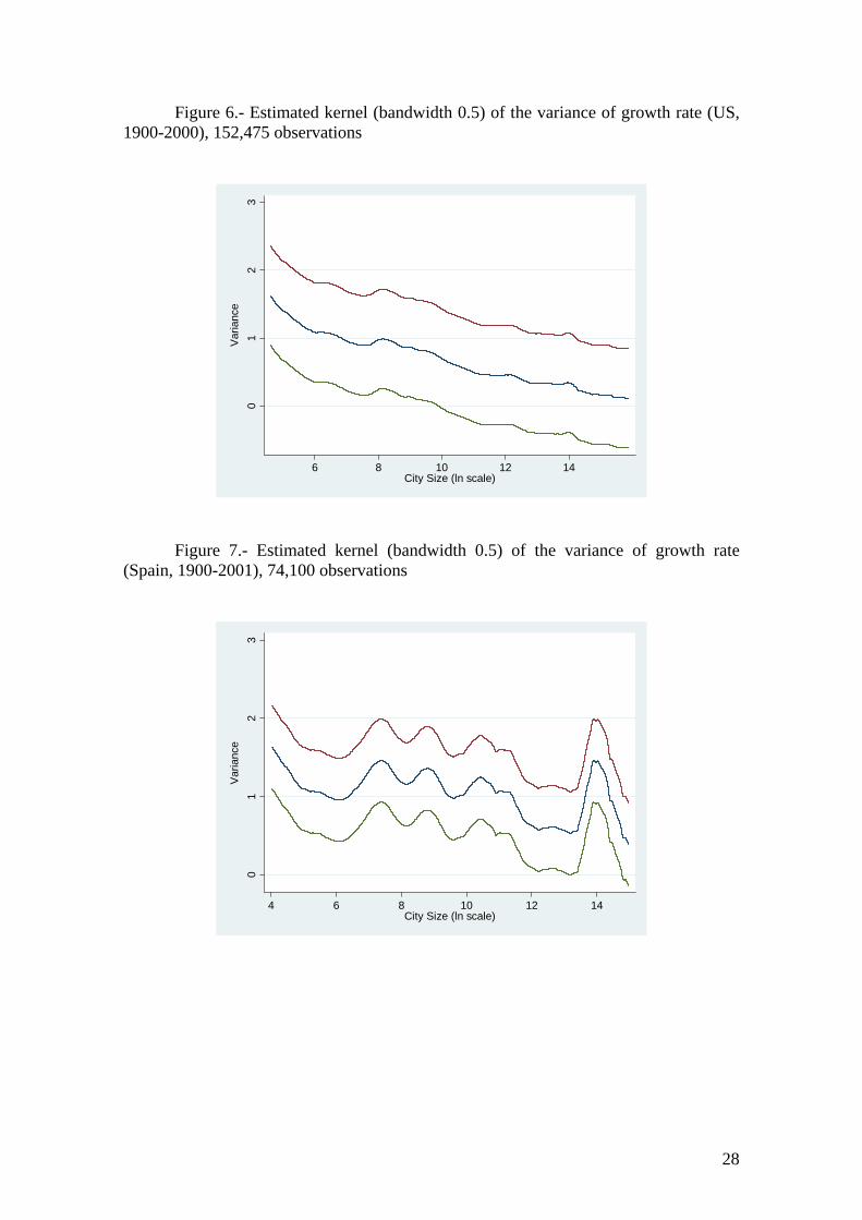
Figures 6, 7 and 8 show the estimated kernels of the variance of growth rate of a pool for the entire 20th century for the US, Spain and Italy, respectively. As expected, while for most of the distribution the value one falls within the confidence bands, indicating that there are no significant differences in variance, the tails of the distribution show differentiated behaviors. In the US the variance clearly decreases with the size of the city, while in Spain and Italy the behavior is more erratic and the biggest cities also have high variance.
To sum up, starting from the estimated kernels of the local means used in this non-parametric section, again the results show that cities of different sizes do not present significant differences in their growth rates, which should lead us to accept Gibrat’s Law, with the evidence being somewhat more favourable in the US than in Spain and Italy. In these last two countries, especially in Spain, the growth rate presents some tendency to growth according to city size.
8. Conclusions
11 This result can be related with the “safe harbour effect” of Edward L. Glaeser and Jesse M. Shapiro (2002), which is a centripetal force which tends to agglomerate the population in large cities when there is an armed conflict.
14
The aim of this work is to test empirically the validity of Gibrat’s Law in the growth of cities, using data for all the twentieth century of the complete distribution of cities (without any size restrictions) in three countries: the US, Spain and Italy.
The first result is that when considering the complete samples, we obtain a tendency to divergence. Despite being three countries with very different urban structures and histories, we find a positive relationship between the growth rate of cities and their initial size throughout the 20th century (except in the period 1970-1980 in the US).
However, the empirical evidence shows that this does not impede city size distribution being approximated as a lognormal distribution. The results of Wilcoxon’s rank-sum test show that the null hypothesis of lognormality is accepted with a significance level of 5% for all periods of the 20th century in Spain and Italy. In the US an evolution over time is observed; in the first decades the lognormal is rejected and the p-value decreases over time, but from 1930 the p-value begins to grow until lognormal distribution is accepted at 5% from 1960 on. But even in these decades the form of the empirical density functions is similar to a lognormal, while we observe a certain concentration of density in the central values of the distribution. In fact, if instead of 5% we take a significance level of 1%, the null hypothesis would only be rejected in 1920 and 1930 in the US.
To resolve this apparent contradiction, which we deduce from our empirical results, between divergent growth and lognormality, we have defined a statistical model, inspired by Kalecki’s [1945] standard framework, which combines lognormality with a variance which grows more than linearly over time.
Moreover, this result of divergent urban growth can and should be qualified in two ways. First, the conclusions obtained in our study depend on the choice of sample size and the inclusion of all cities without size restrictions. When estimating with subsamples and using smaller sample sizes we find there is a critical sample size under which we would always accept the fulfilment of Gibrat’s Law. So, for sample sizes similar to those of other studies, we also accept that Gibrat’s Law holds. And second, the use of non-parametric methods which relate the growth rate with city size through the estimation of local means enable us to observe that in the long term, the evidence in favour of Gibrat's Law increases, especially in the US.
Appendix We have two expressions:
(3) ( ) 2ln σ⋅= tSVar it
( ) ( )ββ
βσ2
11ln 2
22
+−+
⋅=t
itSVar (5)
If Gibrat’s Law is fulfilled ( 0=β ), and applying L'Hôpital’s rule we obtain that (5)
converges to (3): ( ) 2212
221
ββ
++2
0 222lim σσσ
βttt t
==⎟⎟⎠
⎞⎜⎜⎝
⎛⋅
−
→.
Let’s see what happens if 0>β or 0<β :
15
( )( ) ( ) ( )[ ] ( ) ( )[ ]β
ββσβββ
ββσ
βββσσ ftt t
t
2112
2211)5()3(
222
2
2
222
+=++−+
+=
+−+
⋅−⋅=−
Considering time t as a continuum beginning with zero, the expression between brackets
( )βf is only defined if β<−1 . Also, if 0>β then ( ) 02
2
>+ββ
σ , while if 01 <<− β
then ( ) 02
2
<+ββ
σ .
Therefore, to find out the total sign of the difference )5()3( − we must study the behavior of the function ( ) ( ) ( ) 112 22 ++−+= ttf ββββ . The maximum or minimum of this function is obtained by defining the corresponding optimisation problem, whose first order condition is given by:
( ) ( ) ( )( ) 0112 12 =+−+=′= −ttfd
df βββββ ,
From which we deduce that at the extreme ( ) 2211 −+= tβ , which means that ( )βf is maximum or minimum in 0=β . In order to know if the optimum 0=β is maximum or minimum we obtain the second order condition:
( ) ( ) ( )( )( )222
2
11212 −+−−=′′= tttfd
fd ββββ ,
and evaluate the sign in 0=β : ( ) ( ) 0140 <−==′′ ttf β as long as . 1>t
Thus we already know that the function ( )βf is concave and reaches its maximum in 0=β as long as . Considering that 1>t ( )0f =0, this function always takes negative
values except in the maximum.
The final sign of the difference )5 ()3( − will be (maintaining the conditions β< >t
−1and ): 1
1. When 0>β we have seen that ( ) 02
2
>+ββ
σ is fulfilled and city growth is
divergent. The variance of the cities will be bigger than if Gibrat’s Law were fulfilled: )5()3( < .
2. When 0<β city growth is convergent. The variance of the cities will be less than if Gibrat’s Law were fulfilled: )5()3( > .
3. When 0=β (3)=(5).
Acknowledgements The authors would like to thank the Spanish Ministerio de Educación y Ciencia
(SEJ2006-04893/ECON project and AP2005-0168 grant from FPU programme), the DGA (ADETRE research group) and FEDER for their financial support. The comments of Arturo Ramos and members of the ADETRE research group contributed to improving the paper.
16
References [1] Anderson, Gordon, and Ying Ge. 2005. “The Size Distribution of Chinese
Cities.” Regional Science and Urban Economics, 35: 756-776.
[2] Azagra, Joaquín, Pilar Chorén, Francisco J. Goerlich, and Matilde Mas. 2006. La localización de la población española sobre el territorio. Un siglo de cambios: un estudio basado en series homogéneas (1900-2001). Fundación BBVA.
[3] Black, Duncan, and Vernon Henderson. 2003. “Urban Evolution in the USA.” Journal of Economic Geography, 3: 343-372.
[4] Bosker, Maarten, Steven Brakman, Harry Garretsen, and Marc Schramm. 2006. “A Century of Shocks: the Evolution of the German City Size Distribution 1925 – 1999.” CESifo working paper 1728.
[5] Brakman, Steven, Harry Garretsen, and Marc Schramm. 2004. “The Strategic Bombing of German Cities during World War II and its Impact on City Growth.” Journal of Economic Geography, 4: 201-218.
[6] Cheshire, Paul C., and Stefano Magrini. 2004. “Population Growth in European Cities: Weather Matters- but only Nationally.” Regional Studies, 40(1): 23-37.
[7] Clark, J. Stephen, and Jack C. Stabler. 1991. “Gibrat's Law and the Growth of Canadian Cities.” Urban Studies, 28(4): 635-639.
[8] Córdoba, Juan C. Forthcoming. “A generalized Gibrat’s Law for Cities.” International Economic Review.
[9] Davis, Donald R., and David E. Weinstein. 2002. “Bones, Bombs, and Break Points: The Geography of Economic Activity.” American Economic Review, 92(5): 1269-1289.
[10] Duranton, Gilles. 2006. “Some Foundations for Zipf´s Law: Product Proliferation and Local Spillovers.” Regional Science and Urban Economics, 36: 542-563.
[11] Duranton, Gilles. 2007. “Urban Evolutions: The Fast, the Slow, and the Still.” American Economic Review, 97(1): 197-221.
[12] Eaton, Jonathan, and Zvi Eckstein. 1997. “Cities and Growth: Theory and Evidence from France and Japan.” Regional Science and Urban Economics, 27(4–5): 443–474.
[13] Eeckhout, Jan. 2004. “Gibrat's Law for (All) Cities.” American Economic Review, 94(5): 1429-1451.
[14] Eeckhout, Jan. Forthcoming. “Gibrat’s Law for (all) Cities: Reply.” American Economic Review.
[15] Gabaix, Xavier. 1999. “Zipf’s Law for Cities: An Explanation.” Quaterly Journal of Economics, 114(3): 739-767.
[16] Gabaix, Xavier, and Yannis M. Ioannides. 2004. “The Evolution of City Size Distributions.” In Handbook of Urban and Regional Economics, vol. 4, ed. John V. Henderson and Jean. F. Thisse, 2341-2378. Amsterdam: Elsevier Science, North-Holland.
17
[17] Gibrat, Robert. 1931. Les Inégalités Économiques. París: Librairie du Recueil Sirey.
[18] Glaeser, Edward L., and Jesse M. Shapiro. 2002. “Cities and Warfare: The Impact of Terrorism on Urban Form.” Journal of Urban Economics, 51: 205-224.
[19] González-Val, Rafael. 2008. “The Evolution of the US Urban Structure from a Long-run Perspective (1900-2000).” http://mpra.ub.uni-muenchen.de/9732/1/MPRA_paper_9732.pdf.
[20] Guérin-Pace, France. 1995. “Rank-Size Distribution and the Process of Urban Growth.” Urban Studies, 32(3): 551-562.
[21] Härdle, Wolfgang. 1990. “Applied Nonparametric Regression.” In Econometric Society Monographs. Cambridge, New York and Melbourne: Cambridge University Press.
[22] Ioannides, Yannis M., and Henry G. Overman. 2003. “Zipf’s Law for Cities: an Empirical Examination.” Regional Science and Urban Economics, 33: 127-137.
[24] Levy, Moshe. Forthcoming. “Gibrat’s Law for (all) Cities: A Comment.” American Economic Review.
[25] Parr, John B., and Keisuke Suzuki. 1973. “Settlement Populations and the Lognormal Distribution.” Urban Studies, 10: 335-352.
[26] Petrakos, George, Prodromos Mardakis, and Helen Caraveli. 2000. “Recent Developments in the Greek System of Urban Centres.” Environment and Planning B: Planning and Design, 27(2): 169-181.
[27] Resende, Marcelo. 2004. “Gibrat’s Law and the Growth of Cities in Brazil: A Panel Data Investigation.” Urban Studies, 41(8): 1537-1549.
[28] Santarelli, Enrico, Luuk Klomp, and Roy Thurik. 2006. “Gibrat's Law: An Overview of the Empirical Literature.” In Entrepreneurship, Growth, and Innovation: the Dynamics of Firms and Industries, ed. Enrico Santarelli, 41-73. New York: Springer.
[29] Soo, Kwok T. 2007. “Zipf's Law and Urban Growth in Malaysia.” Urban Studies, 44(1): 1-14.
[31] White, Halbert. 1980. “A Heteroskedasticity-Consistent Covariance Matrix Estimator and a Direct Test for Heteroskedasticity.” Econometrica, 48: 817-38.
[32] Zipf, George. 1949. Human Behaviour and the Principle of Least Effort, Cambridge, MA: Addison-Wesley.
18
Tables
Table 1. - Empirical studies on city growth
S C P T S G Etudy ountry eriod runcation point ample size L cIss
E F 1 CC 3 A naton and Eckstein [1997] rance and Japan 1
876-1990 (F) 925-1985 (J)
ities > 50,000 inhabitants (F) ities > 250,000 inhabitants (J) 9 (F), 40 (J) on par (tr mat, lz)
D J 3 A pG 1 C 1 A p
C 1 A p1 C 4 A p
E 1 1 A pI U 1 A 1 A
U 1 A 1 A nB U 1 A 1 R
F 1 C 6 R pM 1 U R p
P 1 U R pW 1 6 M p
A 1 C 1 M pG E
avis and Weinstein [2002] B
apan 1925-1965 Cities > 30,000 inhabitants 03 ar (purt) rakman et al. [2004] ermany
C946-1963 ities > 50,000 inhabitants
7 03 7
ar (purt) lark and Stabler [1991]
Ranada
B975-1984 most populous cities ar (purt)
esende [2004] razil U
980-2000 ities > 1,000 inhabitants A
97 ar (purt) eckhout [2004] S 990-2000 ll cities 9361 ar (gr reg); non par (ker)
noannides and Overman [2003] G
S 900-1990 ll MSAs 12 (1900) to 334 (1990) on par (ker) abaix and Ioannides [2004] S 900-1990 ll MSAs 12 (1900) to 334 (1990) on par (ker)
palack and Henderson [2003] G
S 900-1990 ll MSAs 94 (1900) to 282 (1990) r (purt) uérin-Pace [1995]