MPRAMunich Personal RePEc Archive

Currency Crises During the GreatRecession: Is This Time Different?

Tiziano Arduini and Giuseppe De Arcangelis and Carlo

Leone Del Bello

Sapienza, University of Rome, Sapienza, University of Rome,Sapienza, University of Rome

2011

Online at https://mpra.ub.uni-muenchen.de/36528/MPRA Paper No. 36528, posted 9 February 2012 09:06 UTC

Currency Crises During the Great Recession:Is This Time Different?∗

Tiziano Arduini† Giuseppe De Arcangelis‡ Carlo L. Del Bello§

June 2011

Abstract

During the 2007-2009 financial crisis the foreign exchange market was characterizedby large volatility and wide currency swings. In this paper we evaluate whether duringthe period of the Great Recession there has been a structural break in the relationshipbetween fundamentals and exchange rates within an early-warning framework. This isdone by extending the original data set by Kaminsky and Reinhart (1999) and includingnot only the most recent period, but also 17 new countries. Our analysis considers twovariations of the original early-warning system. First, we propose two new methods toobtain the probability distribution of the early-warning indicator (conditional on theoccurrence of a crisis) – one fully parametric and one based on a novel distribution-freesemi-parametric approach. Second, we compare the original early-warning indicator witha core indicator that includes only “pseudo-financial variables” (domestic credit/GDP,the real exchange rate, international reserves and the real interest-rate differential) andwe evaluate their performance not only for currency crises during the Great Recession,but also for the Asian Crisis. All tests make us conclude that “this time is different”,i.e. early-warning systems based on traditional macroeconomic variables have not onlyfailed to forecast currency crises during the Great Recession, but have also significantlyworsened with respect to the period of the Asian crisis.

Keywords: Early Warning Systems, Exchange Rates, Semi-parametric Meth-ods.

JEL Classification Codes: F31, F47, F30.

∗We wish to thank Gabriele Galati, Ignazio Visco and participants at the conference “Advances in In-ternational Economics and Economic Dynamics – A Conference in Honor of Giancarlo Gandolfo” for usefulcomments on earlier versions of this paper. The usual other disclaimer applies.†Sapienza Universita di Roma‡Dipartimento di Analisi Economiche e Sociali and CIDEI, Sapienza Universita di Roma; e-mail:

g.dearcangelis@caspur.it§Sapienza Universita di Roma

1

Contents

1 Introduction 3

2 Early Warning Systems: the Basics and the Related Literature 52.1 The Market Pressure Index . . . . . . . . . . . . . . . . . . . . . . . . . . . . 52.2 Indicator Variables and the Composite Index . . . . . . . . . . . . . . . . . . . 52.3 The Probability Distribution of the Composite Indicator . . . . . . . . . . . . 72.4 How to Judge EWS Performance . . . . . . . . . . . . . . . . . . . . . . . . . 8

3 A Country-Time Extension of the KR EWS: Critical Issues 103.1 First Issue: Identifying Currency Crises . . . . . . . . . . . . . . . . . . . . . 103.2 Second Issue: How to Compare the Results for the Extended Sample? . . . . . 113.3 Third Issue: Obtaining the Probability Distribution of the Composite Indicator 11

4 The In-Sample Performance of the Original EWS after 1995 124.1 Robustness: Our Replication of the Original KR EWS . . . . . . . . . . . . . 124.2 Country- and Time-Extension: Indications from the Performance of the Origi-

nal EWS . . . . . . . . . . . . . . . . . . . . . . . . . . . . . . . . . . . . . . . 14

5 Advancement 1: A Semi-parametric Approach for the Probability Distri-bution of the Composite Indicator 175.1 Semi-parametric Methods and the Sieve Approach . . . . . . . . . . . . . . . . 185.2 Semi-parametric Methods for Binary-Choice Models and the Khan (2011) Ap-

proach . . . . . . . . . . . . . . . . . . . . . . . . . . . . . . . . . . . . . . . . 20

6 What Insights from Using Different Methods to Obtain the ProbabilityDistribution of the Composite Indicator? 21

7 Advancement 2: An Alternative Pseudo-Financial EWI 23

8 Is There a Structural Break during the Great Recession? 24

9 Conclusions 33

A Description of the Data 37

B Dating the Crises 39

2

1 Introduction

One important aspect of the 2007-2009 financial crisis is the rapid increase in volatility in

the foreign exchange market and the occurrence of large currency swings. Currencies of some

emerging economies depreciated sharply against the dollar and the euro, while capital flows

have been redirected to advanced economies in a typical “flight to safety” phenomenon. For

instance, in September 2008 Ireland and Colombia experienced respectively 22 and 13 per cent

depreciation of their currencies with respect to the dollar. In November 2008 the Korean won

lost 13 per cent of its value with respect to the dollar. In January 2009 Venezuela had a big

drop in its foreign reserves, close to 40 per cent in dollar terms.

These sudden changes indifferently hit countries with very strong fundamentals that had

experienced high GDP growth in the previous years and were following cautious macroe-

conomic policies, as well as other countries with weaker fundamentals. Hence, all types of

currency crises occurred, both self-fulfilling as well as traditional Krugman (1979) type.

The financial crisis has given a new momentum to the literature on the identification of

currency crises and, in particular, to the development of “Early Warning Systems” (EWS).

For instance, the International Monetary Fund and the Financial Stability Board started an

“early warning exercise” in November 20081 and some recent studies have considered the rela-

tionship between the recent financial crisis, international exposure and currency swings (see,

for instance, Obstfeld and Rogoff, 2009, Lane and Milesi-Ferretti, 2010, Shi and Gao, 2010,

Anzuini and Gandolfo, 2003, etc.), while others showed evidence of the difficult predictability

of the recent crisis (see Rose and Spiegel, 2009; Frankel and Saravelos, 2010, provide a recent

survey).

In this paper we deal with two main issues related to the rapid and wide changes in

exchange rates during the period of the Great Recession 2007-2009.

The first issue regards the correct identification of the signal that comes from an early

warning system. More exactly, the original EWS hinges on the construction of a composite

indicator, whose support is simply positive with no upper bound, and the key empirical task is

to obtain the probability of a future crisis associated with the values of the indicator. In this

paper we propose two alternative methods for mapping the (positive and unbounded) values

of the early warning indicator into its conditional distribution. Besides a simple probit model

within the original KLR framework, in this paper we consider a semi-parametric distribution-

free approach, based on Khan (2011), which results particularly suitable for our econometric

framework.

The second issue deals with the dynamics of exchange rates during the Great Recession.

More exactly, we want to evaluate the stability in the relationship between the fundamentals

used in the original early-warning indicators and the exchange rates before and during the

1See <http://www.imf.org/external/np/exr/facts/ewe.htm>.

3

Great Recession. This is done not only by considering structural-stability tests, but also in-

troducing an alternative early-warning indicator based on a core of mainly financial variables

that we name “pseudo-financial indicator” and includes: domestic credit/GDP, the real ex-

change rate, international reserves and the real interest-rate differential. Given the financial

nature of the currency crises in the last two decades, this latter indicator should perform at

least as well as the original wider indicator. Indeed, we evaluate in-sample and out-of-sample

performances of the original and the pseudo-financial indicators. In particular, we compare

their out-of-sample performances not only during the last period, but also for the Asian Cri-

sis. In the end, no striking differences appear between the original and our pseudo-financial

indicator, but both indicators underperform in prediction during the Great Recession with

respect to the Asian crisis. Together with all the other in-sample evidence, we conclude that

the dynamics of exchange rates and their relationships with a large class of common real and

financial fundamentals has changed when judged with their out-of-sample forecasting abilities.

Both analysis are conducted by means of an updated dataset of the original work on EWS

by Kaminsky, Lizondo and Reinhart (1996) and Kaminsky and Reinhart (1999) (henceforth

KLR and KR respectively). More specifically, the original sample of 20 countries is updated

till January 2010 and we included other 17 new countries.

The paper is structured as follows. In Section 2 we summarize the construction of early

warning systems and review part of the literature (this section can be skipped by readers who

are familiar with this approach). Section 3 presents the critical issues when extending the

original dataset and explains our way of dealing with those issues. In Section 4 we present

the in-sample performance of the original KLR system in our new data set after replicating

the original work by KLR. The two original advances of this paper are presented on the next

sections.

First, Section 5 presents intuitively the distribution-free semi-parametric method due to

Khan (2011) to construct the probability distribution of our indicators and Section 6 reports

the performance of the original KLR composite indicator when using alternative methods to

obtain its conditional probability distribution, i.e. the Khan (2011) semi-parametric methods,

our parametric version of the KLR original method and three methods already used in the

literature.

Second, in Section 7 we introduce a new pseudo-financial composite indicator to improve

upon the original KLR indicator in the choice of the relevant macroeconomic variables and we

report its in-sample performance.

Finally, in Section 8 we focus on the out-of-sample performances of the original and the

pseudo-financial indicator by using the different methodologies proposed. We evaluate their

their ability to signal the currency crises during the Asian Crisis in 1997 and the period of the

Great Recession, 2006-2009. Section 9 concludes.

4

2 Early Warning Systems: the Basics and the Related

Literature

The challenge of this strand of literature on Early Warning Systems (EWS) is to find a

sensible combination of variables that could anticipate the occurrence of a crisis. Similarly to

the geological problem of anticipating earthquakes, the main difficulty is to identify variables

that could reliably signal the future occurrence of the event.

However, with more difficulties than for geologists, economists face the problem of correctly

identifying crises in the first place (exchange-rate crisis in our case). Just like geologists

measure earth vibrations and define an “earthquake” as an event where the vibration index

surpasses a certain threshold, similarly economists would define a currency crisis as a situation

when some specific (usually catastrophic) events occur.

However, differently from geologists, economists have to construct the index that would

signal the presence of a currency-crisis and this measure would be less objective than the

measures of earth vibration that geologists use. The construction of this index is key to

identify the events under study and should be inspired by the main exchange-rate models.

2.1 The Market Pressure Index

KLR borrowed the “market pressure index” initially proposed by Eichengreen, Rose and

Wyplosz (1994). The so-called “short” version of this index for country i at time t is given

by:

Ii,t =∆Ei,tEi,t−1

− σE,iσR,i

∆Ri,t

Ri,t−1(1)

where Ei,t is the exchange rate of the currency of country i against the dollar at time t

(quantity of domestic currency per 1 US dollar), Ri,t represents a measure of international

reserves (minus gold) for country i at time t, σE,i and σR,i are the standard deviations of the

monthly percent change, respectively, in the exchange rate and in the reserves. The ratio of

the standard deviations works as an adjusting weight for the different volatilities and for the

different units of measure of the two components of the index.

2.2 Indicator Variables and the Composite Index

Once the index is constructed, the next step is to determine the threshold that would identify a

“currency-crisis” event. KLR proposed to consider a value for the threshold that is 3 standard

deviations above the average of the index over the whole sample, but country-specific.

When the episodes of exchange rate crises are identified, then it is possible to consider

a large set of (macroeconomic) variables whose time-series behavior is thoroughly observed

5

around the crisis episodes in order to uncover which of them is able to anticipate the catas-

trophic event.

Following KLR, many studies have considered the 24-month window that anticipate the ex-

change rate crisis and observed whenever the time series of each variable was showing anoma-

lous variations that could signal the forthcoming event. More specifically, for each of the

selected macroeconomic variables the authors considered the 30 percentiles of their distribu-

tion and observed when each of these percentiles was crossed. This was considered a signal

when the crossing was occurring in the 24-month pre-crisis period or a noise if no crisis was

happening within the next 24 months.

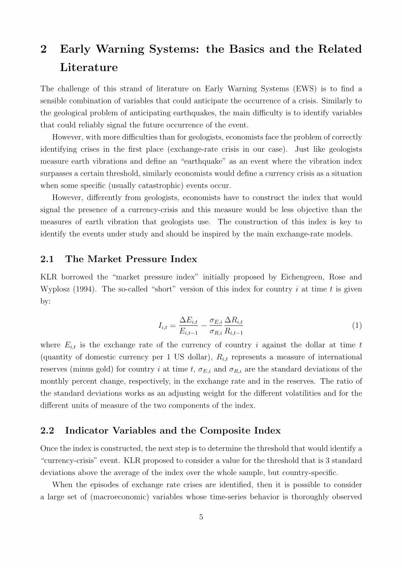
Table 1: Classification of signals and noiseCrisis in the next 24 months No crisis in the next 24 months

Signal Ak,π Bk,π (Type II Error)No signal Ck,π (Type I Error) Dk,π

Table 1 reports how to distribute the number of times each variable crosses the threshold

of the π-th percentile (π = 1, . . . , 30). Hence, Ak,π is the number of times the variable k

crosses the π-th percentile and a crisis occurs in the next 24 months; Dk,π is the number of

times the variable k does not cross the π-th percentile and a crisis does not occur in the next

24 months. In both latter cases our variable (and the relative π-th percentile threshold) is

correctly signaling the crisis or its absence.

The other two cases are instead incorrect signals, or noise. Ck,π and Bk,π are the number of

times the variable k (and the relative threshold associated to the π-th percentile), respectively,

does not signal the crisis when this actually occur and does signal the crisis when this does

not occur in the next 24 months. In other words, they represent respectively type I and type

II error. The key element of this stage is then the noise-to-signal ratio (NSR henceforth)

constructed as follows:

NSRk,π =Bk,π/(Bk,π +Dk,π)

Ak,π/(Ak,π + Ck,π), π = 1, . . . , 30 (2)

KLR call such a scalar “adjusted NSR”.2

The initial aim of the analysis is to identify for each variable k the π-th percentile-threshold

that would minimize the NSR. This is done by pooling the data for all countries. Once

determined the optimal π∗ for each variable, the informational content of all the selected

variables is combined to form a composite indicator that considers the good signals coming

2Berg and Pattillo (1999) note that the optimal threshold does not change if one just minimizes Bk,π/Ak,π,since (Ak,π + Ck,π)/(Bk,π +Dk,π) is a function of the frequency of crises in the data and does not depend onthe threshold.

6

from all the variables (when crossing their optimal thresholds).

In other words, when a variable crosses its own threshold, it issues a warning. But the

fact that two or more variables are signalling a crisis in the same month brings a lot more

information. Kaminsky et al. (1998) proposed the construction of a composite indicator by

summing up all the signals issued by each indicator period by period and adjusted by their

accuracy in terms of NSR. Let us notice that the composite indicator is now country-specific.

More formally, let us be Xk,i,t one of the k = 1, . . . , K signalling macroeconomic variables

for country i at time t and be Xk,i the relative threshold corresponding to the π∗k-th percentile

and the minimum NSR ω∗k. Hence, each variable k issues a crisis signal when Xk,i,t ≥ Xk,i.

This can be mapped into a dichotomic variable Sk,i,t that takes value 1 if a signal is issued at

time t by the variable k for country i.

The composite weighted indicator for country i at time t, Gi,t, is then obtained by summing

up, period by period, all the signals coming from the all the K variables, but weighing them

with their optimal NSR:

Gi,t =K∑i=1

Sk,i,tω∗k

. (3)

2.3 The Probability Distribution of the Composite Indicator

This indicator is a step function with indefinite positive support. The next important step is

to obtain its probability distribution conditional on the event of a crisis within the next 24

months. This is done piecewise and is approximated by the following definition:

P (crisis between time t and (t+24) | Gl < Gt < Gm) = (4)

# months with Gl < Gt < Gm and crisis between time t and (t+24)

# months with Gl < Gt < Gm

where the ranges Gl and Gm are subjectively determined depending on the shape of the

empirical distribution. Once the conditional probability for each arbitrary interval of G is

known, it is also possible to obtain the time series of conditional probabilities by mapping

each value of Gt into its conditional probability.

This can be named as the “complete” KR-KLR EWS. It has the great advantage that it

can issue probability measures of crises in a fully nonparametric approach. However, its main

disadvantage is that it relies on too much craftsmanship by the researcher in the determination

of the probability distribution.

An near alternative EWS is proposed by Berg and Pattillo (1999). Differently from KLR,

it relies on a fully parametric probit specification to generate the conditional probabilities of

crises, but the model selection still hinges on the NSR analysis since the included variables

7

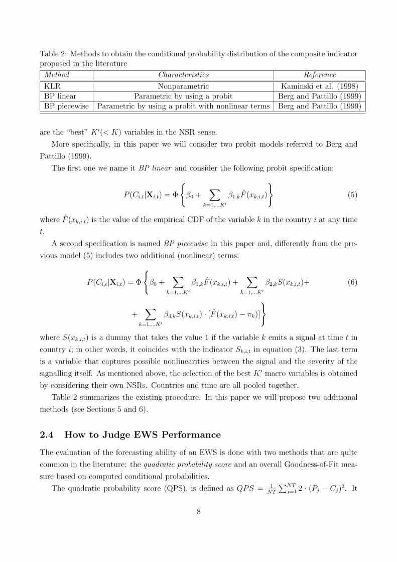
Table 2: Methods to obtain the conditional probability distribution of the composite indicatorproposed in the literature

Method Characteristics Reference

KLR Nonparametric Kaminski et al. (1998)BP linear Parametric by using a probit Berg and Pattillo (1999)BP piecewise Parametric by using a probit with nonlinear terms Berg and Pattillo (1999)

are the “best” K ′(< K) variables in the NSR sense.

More specifically, in this paper we will consider two probit models referred to Berg and

Pattillo (1999).

The first one we name it BP linear and consider the following probit specification:

P (Ci,t|Xi,t) = Φ

β0 +

∑k=1,...K′

β1,kF (xk,i,t)

(5)

where F (xk,i,t) is the value of the empirical CDF of the variable k in the country i at any time

t.

A second specification is named BP piecewise in this paper and, differently from the pre-

vious model (5) includes two additional (nonlinear) terms:

P (Ci,t|Xi,t) = Φ

β0 +

∑k=1,...K′

β1,kF (xk,i,t) +∑

k=1,...K′

β2,kS(xk,i,t)+ (6)

+∑

k=1,...K′

β3,kS(xk,i,t) · [F (xk,i,t)− πk)]

where S(xk,i,t) is a dummy that takes the value 1 if the variable k emits a signal at time t in

country i; in other words, it coincides with the indicator Sk,i,t in equation (3). The last term

is a variable that captures possible nonlinearities between the signal and the severity of the

signalling itself. As mentioned above, the selection of the best K ′ macro variables is obtained

by considering their own NSRs. Countries and time are all pooled together.

Table 2 summarizes the existing procedure. In this paper we will propose two additional

methods (see Sections 5 and 6).

2.4 How to Judge EWS Performance

The evaluation of the forecasting ability of an EWS is done with two methods that are quite

common in the literature: the quadratic probability score and an overall Goodness-of-Fit mea-

sure based on computed conditional probabilities.

The quadratic probability score (QPS), is defined as QPS = 1NT

∑NTj=1 2 · (Pj − Cj)2. It

8

measures how distant the predicted probabilities Pj are (on average with a squared metrics)

from the corresponding realizations (Cj takes value of 1 if there is a crisis at observation j

and zero otherwise). This is an overall measure built with pooled data. A value of zero means

perfect accuracy.

Evaluating the forecasting performance of an EWS means to judge its ability of signalling

correctly the occurrence of a crisis versus tranquil periods. The first question is to determine

when the indicator emits a signal. Given the predicted conditional probability of a crisis at

any given point in time as determined in (4), we need to select an (arbitrary) probability

cutoff τ such that there is a signal of a crisis when this is crossed. Then, in formal terms, a

signal is emitted if P (C|Ω) > τ , where P (C|Ω) is the probability of having a crisis under the

information set Ω and computed as in (4). The probabilities related to all possible events are

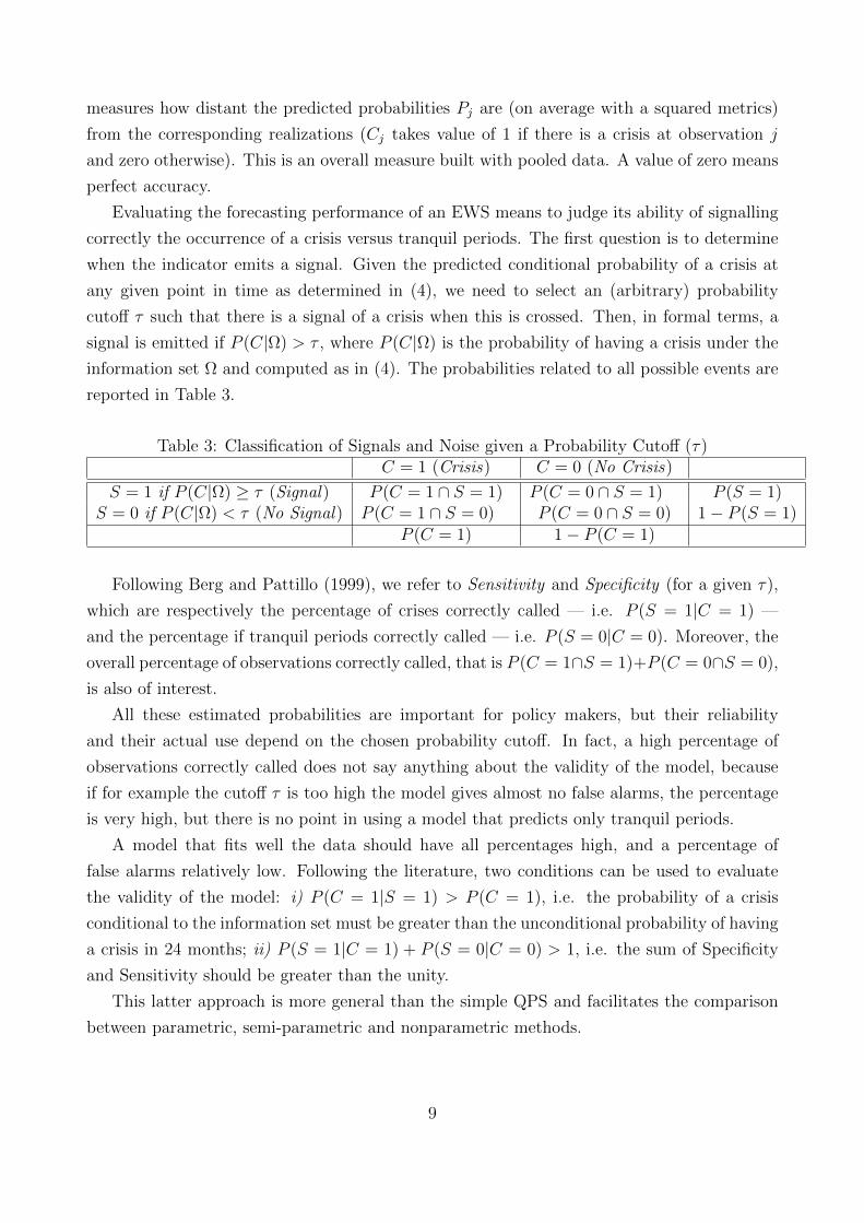
reported in Table 3.

Table 3: Classification of Signals and Noise given a Probability Cutoff (τ)C = 1 (Crisis) C = 0 (No Crisis)

S = 1 if P (C|Ω) ≥ τ (Signal) P (C = 1 ∩ S = 1) P (C = 0 ∩ S = 1) P (S = 1)S = 0 if P (C|Ω) < τ (No Signal) P (C = 1 ∩ S = 0) P (C = 0 ∩ S = 0) 1− P (S = 1)

P (C = 1) 1− P (C = 1)

Following Berg and Pattillo (1999), we refer to Sensitivity and Specificity (for a given τ),

which are respectively the percentage of crises correctly called — i.e. P (S = 1|C = 1) —

and the percentage if tranquil periods correctly called — i.e. P (S = 0|C = 0). Moreover, the

overall percentage of observations correctly called, that is P (C = 1∩S = 1)+P (C = 0∩S = 0),

is also of interest.

All these estimated probabilities are important for policy makers, but their reliability

and their actual use depend on the chosen probability cutoff. In fact, a high percentage of

observations correctly called does not say anything about the validity of the model, because

if for example the cutoff τ is too high the model gives almost no false alarms, the percentage

is very high, but there is no point in using a model that predicts only tranquil periods.

A model that fits well the data should have all percentages high, and a percentage of

false alarms relatively low. Following the literature, two conditions can be used to evaluate

the validity of the model: i) P (C = 1|S = 1) > P (C = 1), i.e. the probability of a crisis

conditional to the information set must be greater than the unconditional probability of having

a crisis in 24 months; ii) P (S = 1|C = 1) + P (S = 0|C = 0) > 1, i.e. the sum of Specificity

and Sensitivity should be greater than the unity.

This latter approach is more general than the simple QPS and facilitates the comparison

between parametric, semi-parametric and nonparametric methods.

9

3 A Country-Time Extension of the KR EWS: Critical

Issues

In this section we consider a series of issues that have been raised when extending the original

KLR sample both in the spatial dimension (i.e. by including 17 new countries) and in the time

dimension (i.e. by considering the more recent period until January 2010). These additions

increase the number of degrees of freedom, but increase also the variability and the diversity

of situations by implying a revision in some parts of the original KLR EWS.

3.1 First Issue: Identifying Currency Crises

As mentioned above, the identification of currency crises is mandated to a “market pressure

index” (MPI) and in particular to its outliers. They were originally identified by KLR as the

time periods when the index crossed the sample average plus three times the sample standard

deviation.

The original dating of all the crises was obtained by KLR not only applying their me-

chanical algorithm, but also including subjectively some crisis episodes that the algorithm

was missing. Indeed, some episodes labeled as crises by KLR-KR are simply not signalled

by the MPI. More specifically, Goldstein, Kaminsky and Reinhart (2003) claim that the MPI

“suggests” the presence of crises, but that their occurrence should actually be identified by

also using institutional data and other sources.

This drawback characterizes also the post-1996 period and our geographically-extended

sample. In particular, some evident episodes of currency crises (e.g. the December 2001

Argentine devaluation) were not signalled by the MPI. We deem that the subjective correction

proposed in the early literature, although necessary to identify all possible known crises, reveals

a failure of the MPI or of its threshold.

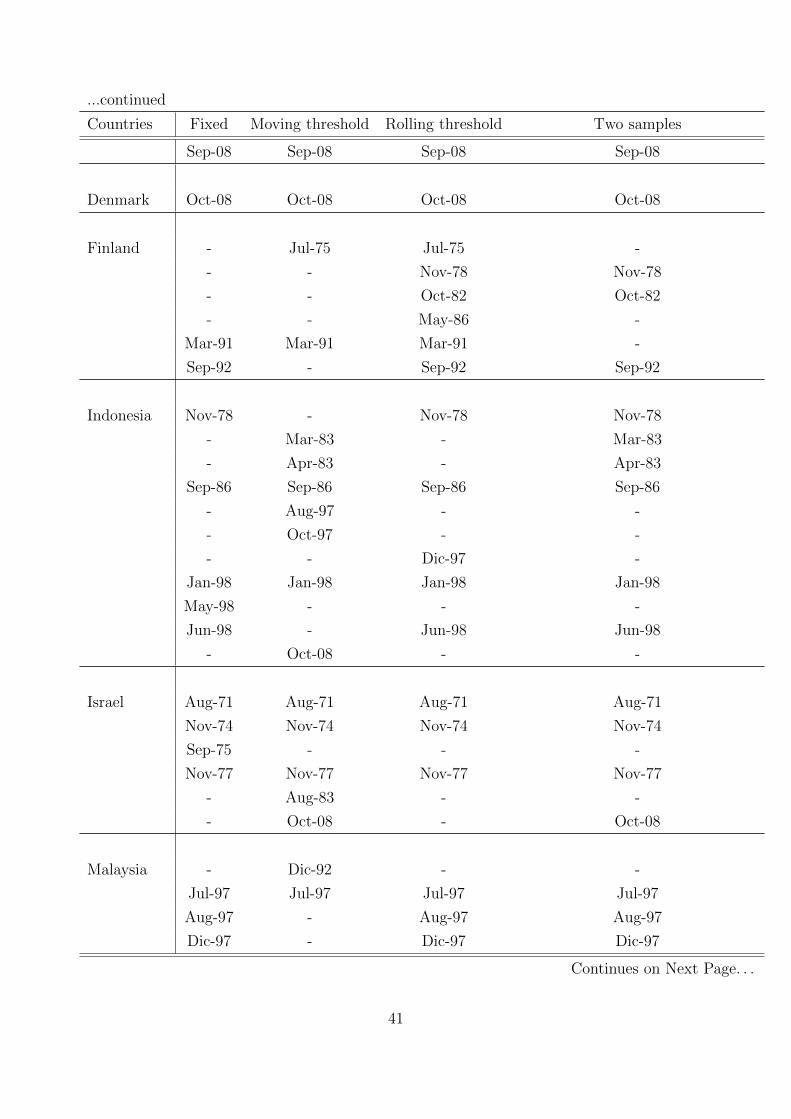
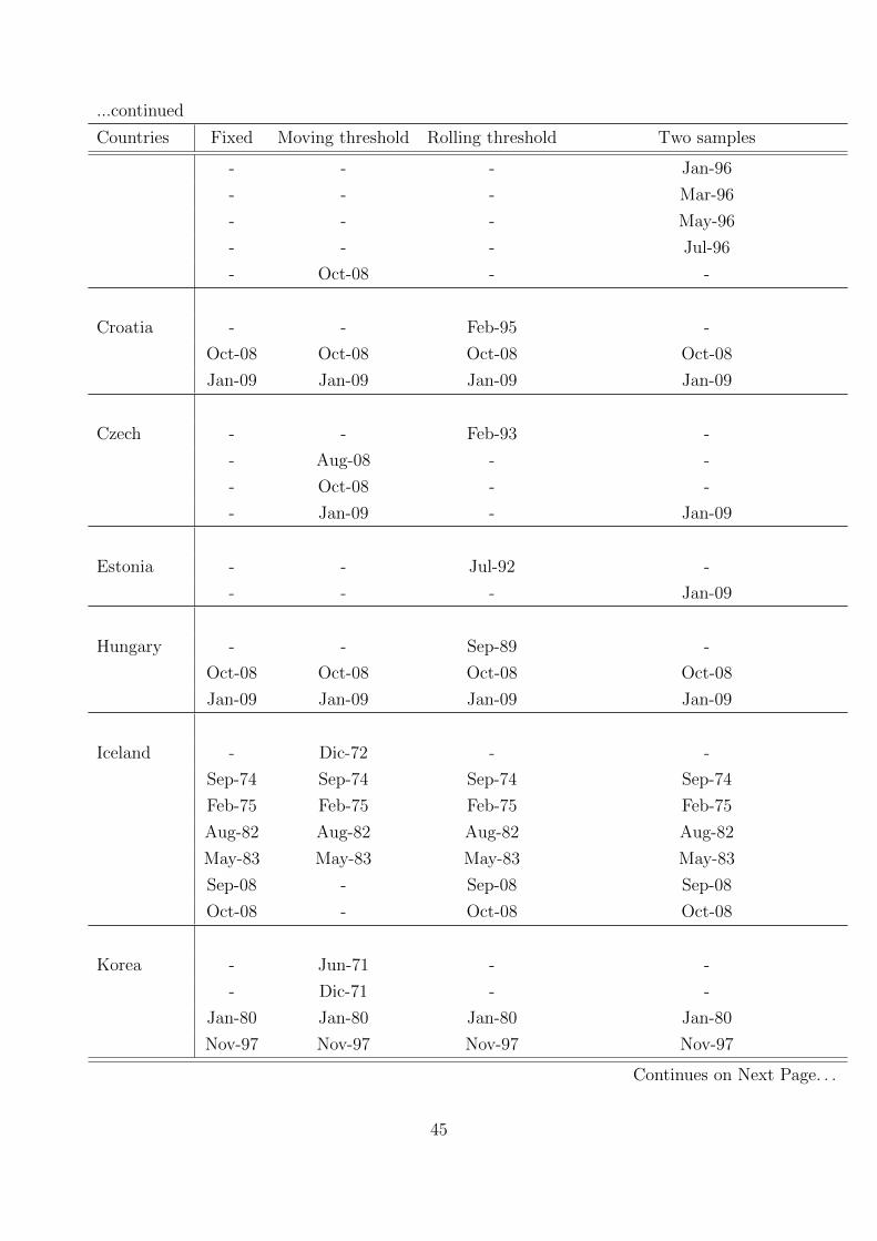
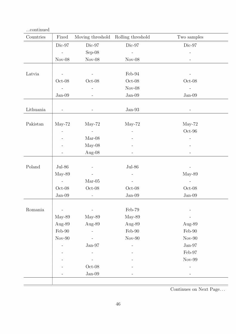
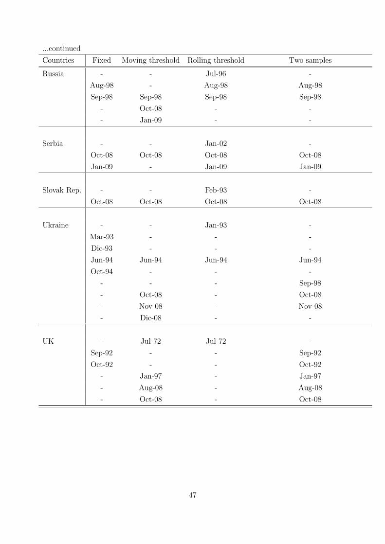
Hence, we explored changes in crisis detection, in particular by varying the determination

of the MPI threshold along two lines in order to take into consideration the longer time span.

First, we considered two time-varying ways of computing mean and standard deviation of the

index and, therefore, the signaling threshold:3 (i) a rolling threshold, by keeping the initial

date (1970:1) fixed and moving the final date period by period; (ii) a moving threshold by

considering a moving window of 60 months to compute the standard deviation. Moreover, we

also considered two separate samples, 1970:1-1981:12 and 1982:1-1996:12.

3We have also changed the level of the threshold by considering two and two and a half standard deviationsabove the mean, as also experimented in other contributions (see Berg et al., 2004). Of course, this variationinduced an increase in the number of crisis episodes. However, it did not improve the average performance ofthe EWS. Results are available from the authors upon request.

10

3.2 Second Issue: How to Compare the Results for the Extended

Sample?

We extend the analysis of the original KLR work by considering a new dataset along two lines,

the time dimension (from 1970-1996 to 1970-2010) and the country dimension (including 17

new countries).4 Would the crisis identification mechanism be robust to this extension? Would

the same algorithm be able to signal the main crises that occurred (according to common

wisdom) after 1996? Which problems of instability may occur by extending the sample in the

first decade of the 21st century and widening the country sample?

We address these questions by considering four subsamples from our full sample (named

FS, including 37 countries from 1970:1 to 2010:1):

• the original KR sample (named KR, with 20 countries from 1970:1 to 1995:12), which is

mainly used to check for robustness with respect to the original analysis;

• the original KR country sample extended till 2010 (named KR+T, with the original 20

countries from 1970:1 to 2010:12) as a simple time extension of the original country set;

• the original KR country sample extended till 2005 (named KR-FOR, with the original

20 countries from 1970:1 to 2005:12) to check the ability to forecast the recent crisis

within the KR sample;

• the full sample till 2005 (named F-FOR, with 37 countries from 1970:1 to 2005:12) to

check the ability to forecast the recent crisis within the larger sample.5

As mentioned in the previous sections, the metrics of our comparison will be centered on

the NSR of each variable included in the EWS and on the changes in the percentile threshold

of each variable, indicating a change in its alert value.

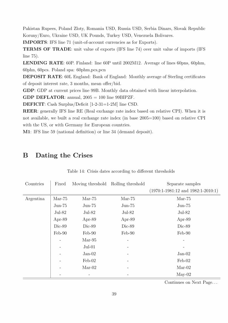
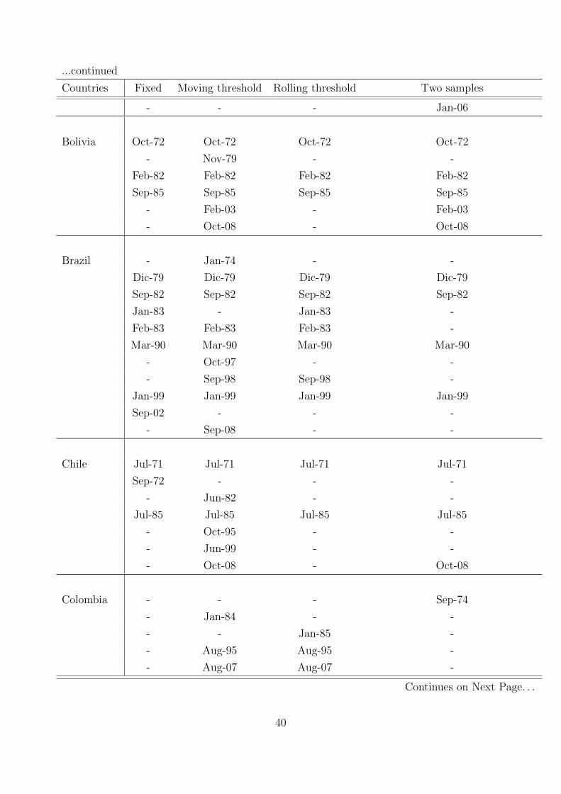
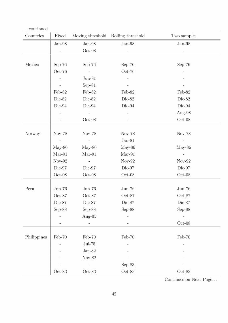
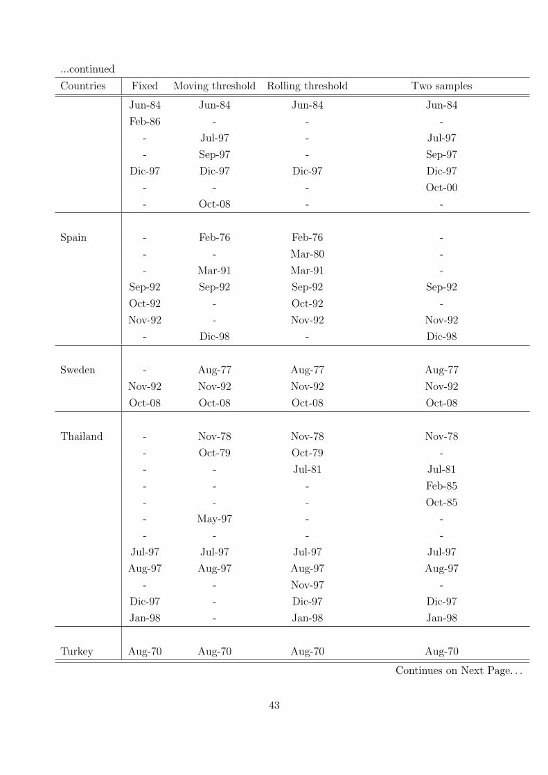
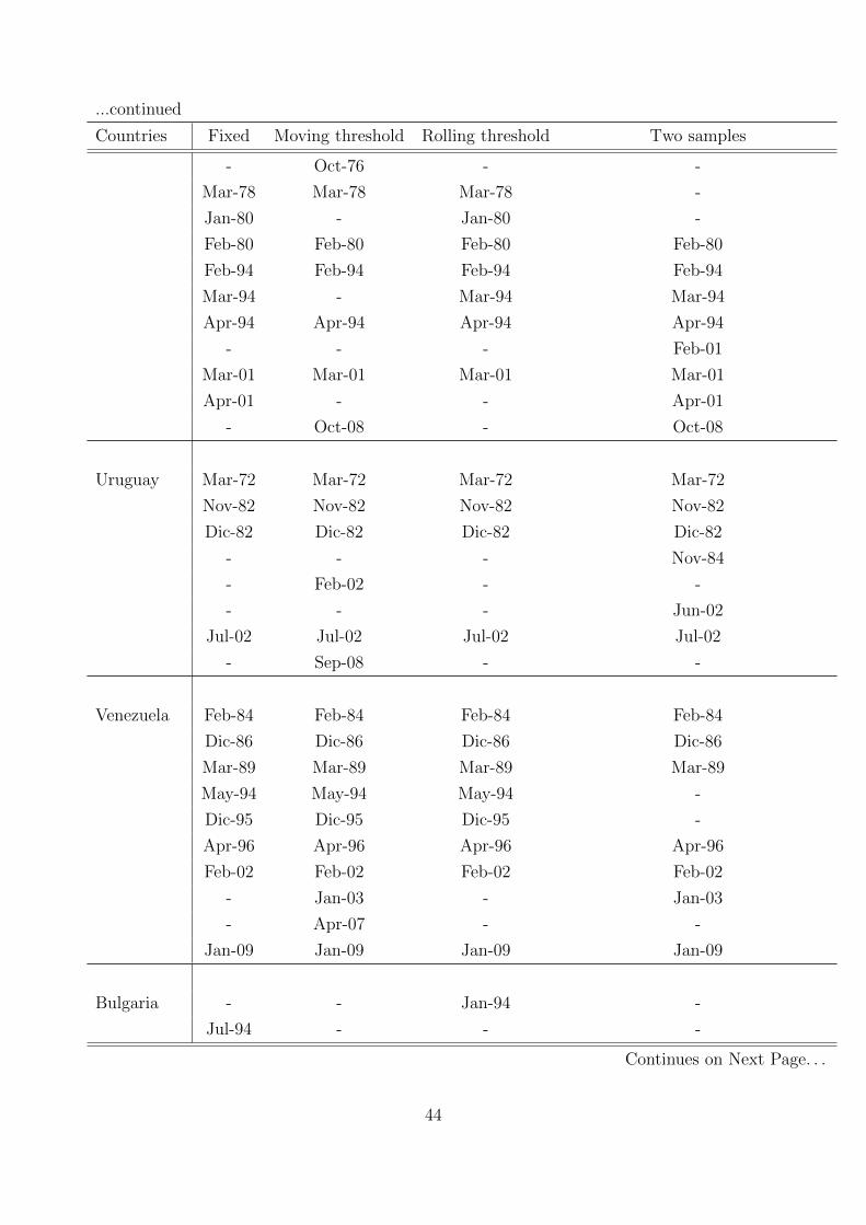
In the new full sample FS the number of crisis episodes increases. Table 14 summarizes the

crisis episodes identified with our methods and compare them with the original KR dating.

3.3 Third Issue: Obtaining the Probability Distribution of the

Composite Indicator

In general, we found that the KR-KLR framework relies too much on “human intervention”

by the researcher. On the contrary, we believe that an EWS should be as much automatic

as possible in order to assure replication and extension. In particular, the mapping from the

4See Appendix A.5The extension of the original KR time sample 1970-1995 to the new 17 countries would not be possible

since most of them are Eastern European countries that either would not exist before the 1990s or were notmarket economies.

11

composite indicator to its conditional probability reported in (4) requires a lot of tailoring work

in choosing the best intervals so as to assure that the probabilities be increasing in G and be

close to the value of 1 when G is at its maximum. In our replication computed probabilities

are not always monotonically increasing and the probability associated to the maximum level

of G remains low, as it is common to other studies.

As an alternative, Berg and Pattillo (1999) propose a probit model with two different

specifications (see Section 2.3 and Table 2).

In this paper, one of the contributions is to improve upon the existing methods to derive

the conditional probability of the composite indicator and we propose two alternatives.

The first one takes a fully parametric approach to obtain the distribution of the indicator

by fitting a pooled probit specification to the crisis indicator Gj (j = 1, . . . NT ):

P (Cj|Gj) = Φ(β0 + β1Gj)

Since this is a mixture of the original KLR method, but adding a probit model to derive

the conditional probability of the composite indicator, we name this method as KLR Probit.

The second method that we propose is based on the semi-parametric approach and is based

on the recent advancement proposed by Khan (2011) for discrete choice models. This will be

presented in Section 5, whereas in the next Section 4 we present the results of our (time and

geographic) extensions with the original KLR before considering the other methods.

4 The In-Sample Performance of the Original EWS af-

ter 1995

In this section we perform a first evaluation of the original EWS proposed by KLR when

extending the sample to the most recent period and to a larger set of countries. Within this

EWS we already get some important indications on its performance in the most recent period.

This is already an important result before considering alternative methods and alternative

indicators.

4.1 Robustness: Our Replication of the Original KR EWS

As a first step of our analysis, we replicate the original work by using the same set of 16

macroeconomic variables proposed in the literature. This is only the starting point of our

analysis before proposing different extensions and considering that the replication of the KR

EWS is not banal. In particular, some specific choices and assumptions have to be clearly

stated:

12

• How to treat missing data. Correcting for missing data is a delicate issue. We decided

to restrict the set of signals only to the “feasible” signals, i.e. to the ones for which data

exists. More exactly, for each indicator we excluded all the observations for which data

did not exist. In terms of entries in Table 1, we excluded entries both in the A field

(i.e. a signal when the crisis occurs) and in the C field (i.e. absence of signal when the

crisis occurs). In other words, we deemed that an indicator could not be blamed for not

signaling a crisis if it does not exist. It is not clear what other authors do.

• The minimum threshold. Another issue is that, since the NSR tends to be increasing

in π, the percentile where to start is a crucial choice. The optimal critical region of

rejection of a tranquil period is generally at the first percentile, or very close to it. But

this leads to thresholds that are too restrictive to be useful for early warning purposes

since they occur too rarely. Also, the empirical quantile tends to have a higher variance

at the tails of the distribution.6 KLR, Berg and Pattillo (1999) and Edison (2000) start

from the 10th percentile, whereas Goldstein, Kaminsky and Reinhart (2000) start from

the first one (while KR do not specify). We decided to start from the 5th percentile

(which yields better results in terms of low average NSR).

We applied our algorithm with the updated dataset and the new list of currency crises

is available in Table 14 in the Appendix. In particular, we report all the crises originally

recorded in KR together with the ones we identify with the fixed threshold and with the

different time-varying methods cited in Section 3.1. As mentioned above, we choose the fixed

threshold method with three standard deviations above the mean for all further analysis.

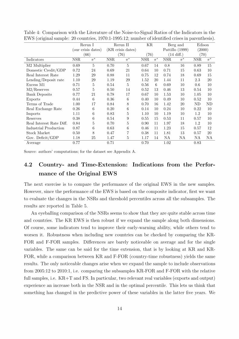
Results of our reruns are provided in Table 4, along with the original results by KR and

previous attempts by other researchers to replicate the same work. In particular, in the

Table we consider two different reruns depending on whether we considered the crisis episodes

identified by our algorithm (Rerun I) or whether considering the original KR dating (Rerun

II).

On average the NSR of the rerun with the KR dates (Rerun II) almost coincides with the

original work (0.71 vs. 0.70), but even when considering the crises identified by our algorithm

(66 instead of 76 in KR) the performance is not very different (0.77 vs. 0.70). These NSR’s

are certainly lower and closer to the original KR’s than the ones obtained by other attempts

in the literature by Berg and Pattillo (1999) and Edison (2000).

We deem that our ability to replicate sufficiently well the original KR contribution of

the macroeconomic indicators (notwithstanding the data revisions and the complexity of the

construction of the dataset) is a good starting point for the rest of the analysis.

6The asymptotic variance of the sample quantile function Q(π) is: AsV ar(Q(π)) = π(1−π)f(Q(π))2 . Hence, it has

a U form and attains a minimum at the median. This means that the asymptotic variance is very large in thetails and it is appropriate to eliminate the first, noisier percentiles.

13

Table 4: Comparison with the Literature of the Noise-to-Signal Ratios of the Indicators in theEWS (original sample: 20 countries, 1970:1-1995:12; number of identified crises in parenthesis).

Rerun I Rerun II KR Berg and Edison(our crisis dates) (KR crisis dates) Pattillo (1999) (2000)

(66) (76) (76) (14 diff.) (70)Indicators NSR π∗ NSR π∗ NSR π∗ NSR π∗ NSR π∗

M2 Multiplier 0.69 5 0.70 5 0.67 14 0.8 16 0.89 15Domestic Credit/GDP 0.72 24 0.69 21 0.64 10 0.71 15 0.63 10Real Interest Rate 1.29 29 0.88 11 0.75 12 0.74 18 0.69 15Lending/Deposit rate 1.10 29 1.19 29 1.52 20 1.44 11 2.3 20Excess M1 0.71 5 0.54 5 0.56 6 0.69 10 0.6 10M2/Reserves 0.57 5 0.50 14 0.52 13 0.46 13 0.54 10Bank Deposits 0.77 21 0.78 17 0.67 10 1.53 10 1.05 10Exports 0.44 6 0.36 6 0.40 10 0.49 10 0.52 10Terms of Trade 1.00 17 0.84 8 0.70 16 1.42 20 ND NDReal Exchange Rate 0.26 6 0.20 6 0.14 10 0.24 10 0.22 10Imports 1.11 6 0.83 5 1.10 10 1.19 10 1.2 10Reserves 0.38 6 0.54 9 0.55 15 0.53 11 0.57 10Real Interest Rate Diff. 0.84 5 0.70 5 0.90 11 1.97 18 1.2 10Industrial Production 0.87 6 0.63 6 0.46 11 1.23 15 0.57 12Stock Market 0.50 8 0.47 7 0.38 11 1.81 13 0.57 20Gov. Deficit/GDP 1.18 25 1.47 5 1.17 14 NA NA NA NAAverage 0.77 0.71 0.70 1.02 0.83

Source: authors’ computations; for the dataset see Appendix A.

4.2 Country- and Time-Extension: Indications from the Perfor-

mance of the Original EWS

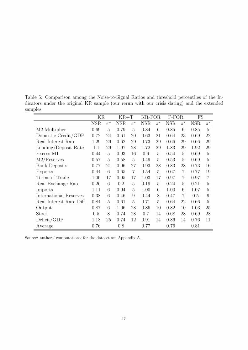
The next exercise is to compare the performance of the original EWS in the new samples.

However, since the performance of the EWS is based on the composite indicator, first we want

to evaluate the changes in the NSRs and threshold percentiles across all the subsamples. The

results are reported in Table 5.

An eyeballing comparison of the NSRs seems to show that they are quite stable across time

and countries. The KR EWS is then robust if we expand the sample along both dimensions.

Of course, some indicators tend to improve their early-warning ability, while others tend to

worsen it. Robustness when including new countries can be checked by comparing the KR-

FOR and F-FOR samples. Differences are barely noticeable on average and for the single

variables. The same can be said for the time extension, that is by looking at KR and KR-

FOR, while a comparison between KR and F-FOR (country-time robustness) yields the same

results. The only noticeable changes arise when we expand the sample to include observations

from 2005:12 to 2010:1, i.e. comparing the subsamples KR-FOR and F-FOR with the relative

full samples, i.e. KR+T and FS. In particular, two relevant real variables (exports and output)

experience an increase both in the NSR and in the optimal percentile. This lets us think that

something has changed in the predictive power of these variables in the latter five years. We

14

Table 5: Comparison among the Noise-to-Signal Ratios and threshold percentiles of the In-dicators under the original KR sample (our rerun with our crisis dating) and the extendedsamples.

KR KR+T KR-FOR F-FOR FSNSR π∗ NSR π∗ NSR π∗ NSR π∗ NSR π∗

M2 Multiplier 0.69 5 0.79 5 0.84 6 0.85 6 0.85 5Domestic Credit/GDP 0.72 24 0.61 20 0.63 21 0.64 23 0.69 22Real Interest Rate 1.29 29 0.62 29 0.73 29 0.66 29 0.66 29Lending/Deposit Rate 1.1 29 1.97 28 1.72 29 1.83 29 1.92 29Excess M1 0.44 5 0.93 16 0.6 5 0.54 5 0.69 5M2/Reserves 0.57 5 0.58 5 0.49 5 0.53 5 0.69 5Bank Deposits 0.77 21 0.96 27 0.93 28 0.83 28 0.73 16Exports 0.44 6 0.65 7 0.54 5 0.67 7 0.77 19Terms of Trade 1.00 17 0.95 17 1.03 17 0.97 7 0.97 7Real Exchange Rate 0.26 6 0.2 5 0.19 5 0.24 5 0.21 5Imports 1.11 6 0.94 5 1.00 6 1.00 6 1.07 5International Reserves 0.38 6 0.46 9 0.44 8 0.47 7 0.5 9Real Interest Rate Diff. 0.84 5 0.61 5 0.71 5 0.64 22 0.66 5Output 0.87 6 1.06 28 0.86 10 0.82 10 1.03 25Stock 0.5 8 0.74 28 0.7 14 0.68 28 0.69 28Deficit/GDP 1.18 25 0.74 12 0.91 14 0.86 14 0.76 11Average 0.76 0.8 0.77 0.76 0.81

Source: authors’ computations; for the dataset see Appendix A.

15

will address this issue in detail in Section 8.

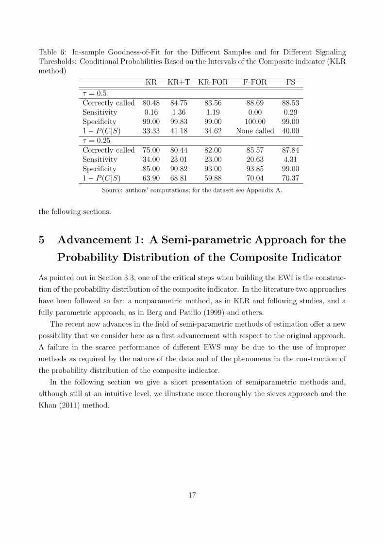
The in-sample performance of the original EWS is reported in Table 6 for two different

values of the signaling threshold (τ equal to 0.25 and 0.50) across all the samples, starting

with the original KR sample to the full sample.

When considering the most conservative threshold at 0.50, the EWS performs well in all the

subsamples, showing an increase in the percentage of correctly called signals and in the general

trustworthiness of the indicator (i.e. a high value in P [C|S]). However, signals activated at

the 50 per cent probability threshold perform well because they correctly call tranquil periods

(see the high value in “Specificity”), but are useless in predicting the occurrence of the crises

(i.e. the value of “Sensitivity” is close to zero).

A more interesting result is obtained when looking at the threshold τ = 0.25.7 In this case

the value of Sensitivity increases and Specificity is still high. Their sum is always higher than

1 for all the samples. In terms of correctly called crises, the extension of the sample along the

time (see both KR+T and KR-FOR) and the country dimension (see F-FOR and FS) seems

to improve the performance. But this is mainly due to the improved ability to predict tranquil

periods rather than crises — especially when comparing FS with all the other subsamples.

At the threshold τ = 0.25 other interesting indications come from Sensitivity and Speci-

ficity. When looking only at the original KR 20 countries, Sensitivity (i.e. the ability of

anticipating crises) is equal to 34 per cent in the original subperiod 1970-1995. Sensitivity

drops in the larger sample 1970-2005 for both the original 20 countries (i.e. KR-FOR subsam-

ple) and the full sample of the 37 countries (i.e. F-FOR subsample), being respectively 23.01

per cent to 20.63 per cent.

However, a much more remarkable fall is observed when including the more recent years

after 2005 in the full sample (FS). Sensitivity collapses to 4.31 per cent. A similar drop is not

observed when considering only the original KR 20 countries in the full sample since Sensitivity

remains equal to 23.01, i.e. very similar to the value for the KR-FOR sample (23). Hence, a

structural break in the performance of the indicator is due to the particular bad performance

for the new countries, but only in the recent years after 2005.

Hence, the lower predictive power of the original KR EWS seems to be attributed to the

bad performance for the new 17 countries in the sample, although their bad contribution is

confined only in the very last period 2006-2010, i.e. the period closely coinciding with the

Great Recession.

Hence, we cannot exclude a generalized failure in the performance of the KR EWS due

to the peculiarity of the post-2005 period. Using alternative methods for the construction

of the conditional probability distribution of the composite indicator (Sections 5 and 6) or

introducing a new, more-focused indicator (Section 7), may give more insights as presented in

7The choice of this threshold is due also to facilitate comparison with literature

16

Table 6: In-sample Goodness-of-Fit for the Different Samples and for Different SignalingThresholds: Conditional Probabilities Based on the Intervals of the Composite indicator (KLRmethod)

KR KR+T KR-FOR F-FOR FS

τ = 0.5Correctly called 80.48 84.75 83.56 88.69 88.53Sensitivity 0.16 1.36 1.19 0.00 0.29Specificity 99.00 99.83 99.00 100.00 99.001− P (C|S) 33.33 41.18 34.62 None called 40.00τ = 0.25Correctly called 75.00 80.44 82.00 85.57 87.84Sensitivity 34.00 23.01 23.00 20.63 4.31Specificity 85.00 90.82 93.00 93.85 99.001− P (C|S) 63.90 68.81 59.88 70.04 70.37

Source: authors’ computations; for the dataset see Appendix A.

the following sections.

5 Advancement 1: A Semi-parametric Approach for the

Probability Distribution of the Composite Indicator

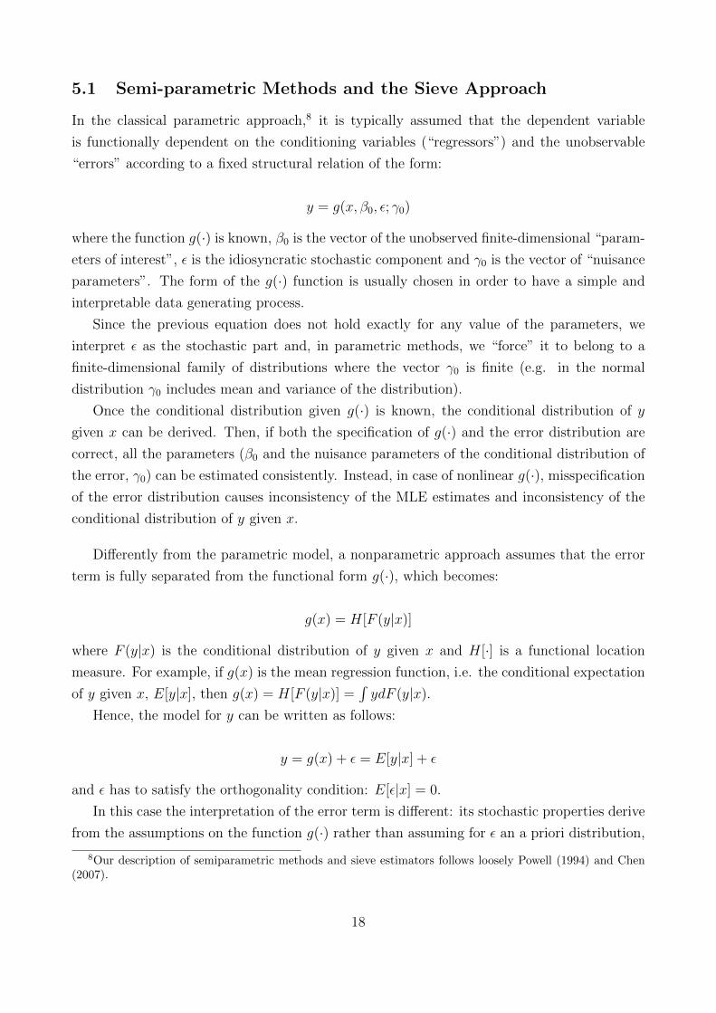
As pointed out in Section 3.3, one of the critical steps when building the EWI is the construc-

tion of the probability distribution of the composite indicator. In the literature two approaches

have been followed so far: a nonparametric method, as in KLR and following studies, and a

fully parametric approach, as in Berg and Patillo (1999) and others.

The recent new advances in the field of semi-parametric methods of estimation offer a new

possibility that we consider here as a first advancement with respect to the original approach.

A failure in the scarce performance of different EWS may be due to the use of improper

methods as required by the nature of the data and of the phenomena in the construction of

the probability distribution of the composite indicator.

In the following section we give a short presentation of semiparametric methods and,

although still at an intuitive level, we illustrate more thoroughly the sieves approach and the

Khan (2011) method.

17

5.1 Semi-parametric Methods and the Sieve Approach

In the classical parametric approach,8 it is typically assumed that the dependent variable

is functionally dependent on the conditioning variables (“regressors”) and the unobservable

“errors” according to a fixed structural relation of the form:

y = g(x, β0, ε; γ0)

where the function g(·) is known, β0 is the vector of the unobserved finite-dimensional “param-

eters of interest”, ε is the idiosyncratic stochastic component and γ0 is the vector of “nuisance

parameters”. The form of the g(·) function is usually chosen in order to have a simple and

interpretable data generating process.

Since the previous equation does not hold exactly for any value of the parameters, we

interpret ε as the stochastic part and, in parametric methods, we “force” it to belong to a

finite-dimensional family of distributions where the vector γ0 is finite (e.g. in the normal

distribution γ0 includes mean and variance of the distribution).

Once the conditional distribution given g(·) is known, the conditional distribution of y

given x can be derived. Then, if both the specification of g(·) and the error distribution are

correct, all the parameters (β0 and the nuisance parameters of the conditional distribution of

the error, γ0) can be estimated consistently. Instead, in case of nonlinear g(·), misspecification

of the error distribution causes inconsistency of the MLE estimates and inconsistency of the

conditional distribution of y given x.

Differently from the parametric model, a nonparametric approach assumes that the error

term is fully separated from the functional form g(·), which becomes:

g(x) = H[F (y|x)]

where F (y|x) is the conditional distribution of y given x and H[·] is a functional location

measure. For example, if g(x) is the mean regression function, i.e. the conditional expectation

of y given x, E[y|x], then g(x) = H[F (y|x)] =∫ydF (y|x).

Hence, the model for y can be written as follows:

y = g(x) + ε = E[y|x] + ε

and ε has to satisfy the orthogonality condition: E[ε|x] = 0.

In this case the interpretation of the error term is different: its stochastic properties derive

from the assumptions on the function g(·) rather than assuming for ε an a priori distribution,

8Our description of semiparametric methods and sieve estimators follows loosely Powell (1994) and Chen(2007).

18

as in the parametric case.

A suitable estimator of g(·) (for a sample of n observations) is:

gn = H[Fn(y|x)]

where the functional H[·] is known (it was the operator “expected value” above). In the non-

parametric approach the main problem is an efficient estimation of the conditional distribution

function of y given x, i.e. Fn(y|x).

The main advantage of nonparametric models is that they impose few restrictions on the

form of the joint distribution of the data and so the misspecification of the functional form is

less likely. On the other hand, the precision of the estimators based only on nonparametric

restrictions is often poor. For example, when you estimates g(·) by smoothing the empirical

cumulative distribution function (CDF) of the data, the rate of convergence is slower than in

the parametric case because of the bias caused by the smoothing.

The semi-parametric approach is halfway between the two latter models since it considers

jointly the regressors and the error term within the function g(·), as in the parametric case,

but treats separately the behavior of the errors.

In a semi-parametric model we consider two components: the “parameters of interest” that

link x to y, which are finite-dimensional, and nuisance functions related to the distribution of

the error term, which are treated nonparametrically. More formally:

y = g (x, β0, ε; γ(·))

where β0 is the unknown vector of parameters of interest that belongs to a finite-dimensional

Euclidian subspace; γ(·) represents the nuisance functions that, differently from the parametric

case, are unknown — or, said differently, involve the knowledge of nuisance parameters that

lie in infinite-dimensional spaces.

In other words, in the semi-parametric approach the y–x relationship can be considered

“parametric”, whereas the error term characteristics are fully nonparametric.

It has been shown that it is possible to obtain consistent estimates of the nuisance pa-

rameters, although belonging to infinite-dimensional spaces, by means of the optimization

of a criterion function that uses finite samples. This approach is named “sieve” since the

approximation of the infinite-dimensional space is operated with less complex – and often

finite-dimensional – parameter spaces that are called “sieves” (see Chen, 2007).

19

5.2 Semi-parametric Methods for Binary-Choice Models and the

Khan (2011) Approach

Manski (1975, 1985) used a semi-parametric method to estimate binary choice models, which

is the class of econometric models we are using in this paper. He solved the main problems

related to these models, i.e. the inconsistency of the estimators under both heteroskedastic

conditional error terms and misspecification of the error distribution. The identification of

the parameters of interest β0 is obtained by imposing that the conditional median be zero

(conditional-median-restriction estimator).

However, the Manski (1975, 1985) approach has three main problems. First, it does not

estimate choice probabilities. Second, it is very difficult to implement since the criterion

function is not smooth. Third, it does not have good statistical properties (i.e. slow rate of

convergence of the estimators and non-Gaussian limiting distribution).9

Khan (2011) proposes the application of the sieve approach to the binary choice models by

using a “distribution-free” binary response estimator with a manageable implementation.10

Khan (2011) has shown that the binary response model yi = Ix′iβ − εi (where I(·) is

an indicator function) with a null conditional-median restriction for identification is “obser-

vationally” equivalent11 to a multiplicative heteroskedastic probit (or logit) model up to an

unknown infinite-parameter scale function.

By using the sieve approach described above, the empirical implementation of Khan

(2011)’s result is possible by the definition of a simple empirical criterion function. In partic-

ular, over the sample of n observations the estimator αn of all the parameters can be obtained

by means of nonlinear least squares (NLLS) according to the following:

αn = minα

1

n

n∑i=1

yi − Φ [x′iβ · γn(xi)] ,

where γn(x) is the sieve base and, according to Khan (2011), this can be computed as an

exponential function where the argument is any polynomial of the dependent variables; Φ is

the normal CDF. The estimated vector αn contains both the estimates of β0 and the nuisance

parameters of the exponential γn(x) that approximates the unknown “nuisance functions”

γ(·). Choice probabilities can then be easily computed and are shown to be consistent.

More specifically, in this paper we estimate model (5), i.e. similar to BP linear but with

a semi-parametric approach to estimation.

9Horowitz (1992) proposed a new approach by improving the implementation of the estimation procedurewith a Gaussian limiting distribution.

10See Blevins and Khan (2010) for the actual implementation in Stata.11That is, P (yi = 1|xi = x) is the same in both models.

20

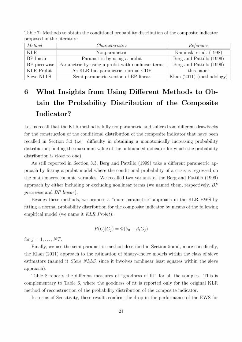
Table 7: Methods to obtain the conditional probability distribution of the composite indicatorproposed in the literature

Method Characteristics Reference

KLR Nonparametric Kaminski et al. (1998)BP linear Parametric by using a probit Berg and Pattillo (1999)BP piecewise Parametric by using a probit with nonlinear terms Berg and Pattillo (1999)KLR Probit As KLR but parametric, normal CDF this paperSieve NLLS Semi-parametric version of BP linear Khan (2011) (methodology)

6 What Insights from Using Different Methods to Ob-

tain the Probability Distribution of the Composite

Indicator?

Let us recall that the KLR method is fully nonparametric and suffers from different drawbacks

for the construction of the conditional distribution of the composite indicator that have been

recalled in Section 3.3 (i.e. difficulty in obtaining a monotonically increasing probability

distribution; finding the maximum value of the unbounded indicator for which the probability

distribution is close to one).

As still reported in Section 3.3, Berg and Pattillo (1999) take a different parametric ap-

proach by fitting a probit model where the conditional probability of a crisis is regressed on

the main macroeconomic variables. We recalled two variants of the Berg and Pattillo (1999)

approach by either including or excluding nonlinear terms (we named them, respectively, BP

piecewise and BP linear).

Besides these methods, we propose a “more parametric” approach in the KLR EWS by

fitting a normal probability distribution for the composite indicator by means of the following

empirical model (we name it KLR Probit):

P (Cj|Gj) = Φ(β0 + β1Gj)

for j = 1, . . . , NT .

Finally, we use the semi-parametric method described in Section 5 and, more specifically,

the Khan (2011) approach to the estimation of binary-choice models within the class of sieve

estimators (named it Sieve NLLS, since it involves nonlinear least squares within the sieve

approach).

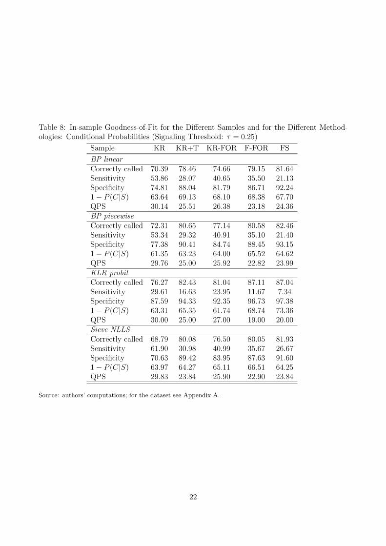
Table 8 reports the different measures of “goodness of fit” for all the samples. This is

complementary to Table 6, where the goodness of fit is reported only for the original KLR

method of reconstruction of the probability distribution of the composite indicator.

In terms of Sensitivity, these results confirm the drop in the performance of the EWS for

21

Table 8: In-sample Goodness-of-Fit for the Different Samples and for the Different Method-ologies: Conditional Probabilities (Signaling Threshold: τ = 0.25)

Sample KR KR+T KR-FOR F-FOR FS

BP linearCorrectly called 70.39 78.46 74.66 79.15 81.64Sensitivity 53.86 28.07 40.65 35.50 21.13Specificity 74.81 88.04 81.79 86.71 92.241− P (C|S) 63.64 69.13 68.10 68.38 67.70QPS 30.14 25.51 26.38 23.18 24.36BP piecewiseCorrectly called 72.31 80.65 77.14 80.58 82.46Sensitivity 53.34 29.32 40.91 35.10 21.40Specificity 77.38 90.41 84.74 88.45 93.151− P (C|S) 61.35 63.23 64.00 65.52 64.62QPS 29.76 25.00 25.92 22.82 23.99KLR probitCorrectly called 76.27 82.43 81.04 87.11 87.04Sensitivity 29.61 16.63 23.95 11.67 7.34Specificity 87.59 94.33 92.35 96.73 97.381− P (C|S) 63.31 65.35 61.74 68.74 73.36QPS 30.00 25.00 27.00 19.00 20.00Sieve NLLSCorrectly called 68.79 80.08 76.50 80.05 81.93Sensitivity 61.90 30.98 40.99 35.67 26.67Specificity 70.63 89.42 83.95 87.63 91.601− P (C|S) 63.97 64.27 65.11 66.51 64.25QPS 29.83 23.84 25.90 22.90 23.84

Source: authors’ computations; for the dataset see Appendix A.

22

the full sample with respect to all the other samples. Differently from Table 6 we note a

systematic fall in sensitivity between 2006 and 2010, not only for the samples that include all

37 countries (i.e. F-FOR and FS), but also for the sample that include only the original KLR

20 countries (i.e. KR-FOR and KR+T).

Hence, the peculiarity of the last years around the Great Recession, independently on the

geographical sample (i.e. either including or excluding the new 17 countries), seems to be

confirmed by these latter results. The next experiment would be to consider an alternative

composite indicators and see whether there can be an improvement in the predictability of

currency crises with a different set of variables.

7 Advancement 2: An Alternative Pseudo-Financial EWI

In the Section 6 we have shown that, when using alternative methods for the construction of

the probability distribution of the composite indicator, the EWS dramatically underperforms

in the last period 2006-2010.

In this section we want to analyze whether the weakness of the EWS depends on the fact

that too many irrelevant variables are contributing to the formation of the composite indicator,

hence introducing too much noise.

Following the same steps as in the construction of a composite indicator, we then formed an

alternative early warning indicator (EWI) that would focus on the best-performing (in terms of

average NSR) pseudo-financial variables. More exactly, we considered: domestic credit/GDP,

the real exchange rate, international reserves and the real interest-rate differential.

This new EWI combines both pure financial variables (like Domestic Credit/GDP and

International Reserves) and real variables that we name “pseudo-financial” (i.e. the real

exchange rate and the real interest-rate differential) since they are highly affected by their

nominal component in the short run. The increasing importance of financial flows in the

last two decades and the financial nature of the Great Recession are the additional, sensible

reasons why to confine our indicator to these determinants.

Moreover, knowing in advance the NSR of all the variables that compose our pseudo-

financial indicator, we are aware to select what could be the best of all possible alternative

financial indicators ex post.

In other words, we are playing an unfair game knowing that the pseudo-financial indicator

is including only the best macroeconomic variables. However, this is done on purpose to

improve our EWS along the dimension of the best information set. We recall that our main

purpose is to evaluate the stability of the relationship between the fundamentals and the

exchange rates. Our new indicator should be the best on average, but our question is whether

23

this is true all over the sample including the period of the Great Recession.

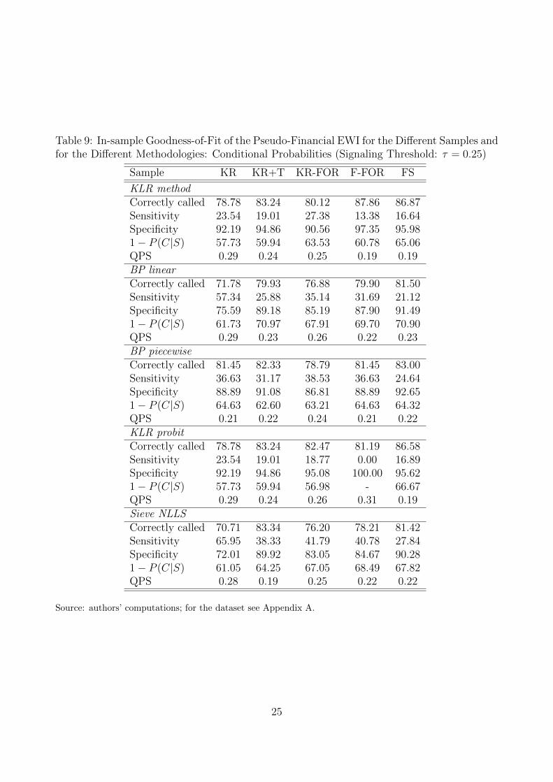
Table 9 reports the various indexes of performance for all our samples and for all methods

to obtain the probability distribution of the new composite index.

As expected, the general performance of the new composite index improves according to the

QPS and the probability of having a crisis when it is signalled (i.e. P [C|S]). More interesting is

the comparison between the performances in terms of Sensitivity in the subsamples, especially

KR-FOR vs. KR+T and F-FOR vs. FS, recalling that there was a sensitive decrease when

including the last four years with the original composite indicators.

This latter result seems to be generally confirmed. This is consistently observed between

KR-FOR and KR+T (except for KLR Probit for which there is a very slight improvement).

Hence, with the original KR 20 countries, the last four years show a break even in the perfor-

mance of the pseudo-financial indicator.

The same can be said also for the larger new sample of 37 countries when considering three

out of five methods. Only when considering the original KLR method and its slight parametric

variation (KLR Probit) there is an improvement in the Sensitivity of the new pseudo-financial

indicator in the full sample.

Finally, we ought to notice that, just like in the case of original EWS (in Table 8), the

distribution-free semi-parametric method (Sieve NLLS) performs best with respect to Sensi-

tivity.

8 Is There a Structural Break during the Great Reces-

sion?

The empirical results shown thus far indicate that there is a discontinuity in the last four years

of our sample. The performance of the composite indicator as an early-warning indicator seems

to get worse when including the years 2006-2009 and this is confirmed when considering not

only different methodologies in the (very sensitive) construction of the probability distribution

of the composite indicators (Section 6), but also when choosing an ad-hoc well-performing

pseudo-financial indicator (Section 7).

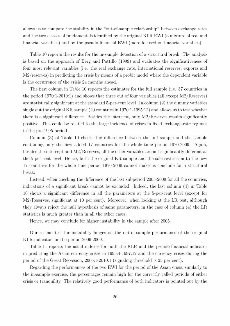
In this section we test formally the presence of a structural break in two different ways.

First, we check whether there is instability in a probit model a la Berg-Pattillo (1999) by

adding dummy variables for the different sample extensions. We focus on results for the time

extension 2006-2009.

Next, we evaluate the out-of-sample performance of the original KLR EWS for the last

period 2006-2009 and we compare it along two lines: first, with its out-of-sample performance

for the Asian Crisis; secondly, with the out-of-sample performance of the pseudo-financial

indicator (for both the Asian Crisis and the Great Recession period). This latter analysis

24

Table 9: In-sample Goodness-of-Fit of the Pseudo-Financial EWI for the Different Samples andfor the Different Methodologies: Conditional Probabilities (Signaling Threshold: τ = 0.25)

Sample KR KR+T KR-FOR F-FOR FS

KLR methodCorrectly called 78.78 83.24 80.12 87.86 86.87Sensitivity 23.54 19.01 27.38 13.38 16.64Specificity 92.19 94.86 90.56 97.35 95.981− P (C|S) 57.73 59.94 63.53 60.78 65.06QPS 0.29 0.24 0.25 0.19 0.19BP linearCorrectly called 71.78 79.93 76.88 79.90 81.50Sensitivity 57.34 25.88 35.14 31.69 21.12Specificity 75.59 89.18 85.19 87.90 91.491− P (C|S) 61.73 70.97 67.91 69.70 70.90QPS 0.29 0.23 0.26 0.22 0.23BP piecewiseCorrectly called 81.45 82.33 78.79 81.45 83.00Sensitivity 36.63 31.17 38.53 36.63 24.64Specificity 88.89 91.08 86.81 88.89 92.651− P (C|S) 64.63 62.60 63.21 64.63 64.32QPS 0.21 0.22 0.24 0.21 0.22KLR probitCorrectly called 78.78 83.24 82.47 81.19 86.58Sensitivity 23.54 19.01 18.77 0.00 16.89Specificity 92.19 94.86 95.08 100.00 95.621− P (C|S) 57.73 59.94 56.98 - 66.67QPS 0.29 0.24 0.26 0.31 0.19Sieve NLLSCorrectly called 70.71 83.34 76.20 78.21 81.42Sensitivity 65.95 38.33 41.79 40.78 27.84Specificity 72.01 89.92 83.05 84.67 90.281− P (C|S) 61.05 64.25 67.05 68.49 67.82QPS 0.28 0.19 0.25 0.22 0.22

Source: authors’ computations; for the dataset see Appendix A.

25

allows us to compare the stability in the “out-of-sample relationship” between exchange rates

and the two classes of fundamentals identified by the original KLR EWI (a mixture of real and

financial variables) and by the pseudo-financial EWI (more focused on financial variables).

Table 10 reports the results for the in-sample detection of a structural break. The analysis

is based on the approach of Berg and Pattillo (1999) and evaluates the significativeness of

four most relevant variables (i.e. the real exchange rate, international reserves, exports and

M2/reserves) in predicting the crisis by means of a probit model where the dependent variable

is the occurrence of the crisis 24 months ahead.

The first column in Table 10 reports the estimates for the full sample (i.e. 37 countries in

the period 1970:1-2010:1) and shows that three out of four variables (all except M2/Reserves)

are statistically significant at the standard 5-per-cent level. In column (2) the dummy variables

single out the original KR sample (20 countries in 1970:1-1995:12) and allows us to test whether

there is a significant difference. Besides the intercept, only M2/Reserves results significantly

positive. This could be related to the large incidence of crises in fixed exchange-rate regimes

in the pre-1995 period.

Column (3) of Table 10 checks the difference between the full sample and the sample

containing only the new added 17 countries for the whole time period 1970-2009. Again,

besides the intercept and M2/Reserves, all the other variables are not significantly different at

the 5-per-cent level. Hence, both the original KR sample and the sole restriction to the new

17 countries for the whole time period 1970-2009 cannot make us conclude for a structural

break.

Instead, when checking the difference of the last subperiod 2005-2009 for all the countries,

indications of a significant break cannot be excluded. Indeed, the last column (4) in Table

10 shows a significant difference in all the parameters at the 5-per-cent level (except for

M2/Reserves, significant at 10 per cent). Moreover, when looking at the LR test, although

they always reject the null hypothesis of same parameters, in the case of column (4) the LR

statistics is much greater than in all the other cases.

Hence, we may conclude for higher instability in the sample after 2005.

Our second test for instability hinges on the out-of-sample performance of the original

KLR indicator for the period 2006-2009.

Table 11 reports the usual indexes for both the KLR and the pseudo-financial indicator

in predicting the Asian currency crises in 1995:4-1997:12 and the currency crises during the

period of the Great Recession, 2006:1-2010:1 (signaling threshold is 25 per cent).

Regarding the performances of the two EWI for the period of the Asian crisis, similarly to

the in-sample exercise, the percentages remain high for the correctly called periods of either

crisis or tranquility. The relatively good performance of both indicators is pointed out by the

26

Table 10: Probit estimates. Full sample, indicators in percentile

(1) (2) (3) (4)VARIABLES

Real exchange rate -0.713*** -0.745*** -0.736*** -1.237***(0.0542) (0.0617) (0.0612) (0.0668)

Reserves -0.488*** -0.557*** -0.577*** -0.539***(0.0800) (0.0872) (0.0862) (0.0893)

Exports -0.378*** -0.418*** -0.446*** -0.496***(0.0569) (0.0642) (0.0634) (0.0658)

M2/Reserves -0.110 -0.293*** -0.222*** -0.338***(0.0769) (0.0854) (0.0840) (0.0893)

D KR sample -0.918***(0.120)

dKR*RER 0.244*(0.138)

dKR*Res 0.251(0.230)

dKR*Exp 0.139(0.146)

dKR*M2/Res 0.926***(0.211)

D new sample -0.833***(0.125)

dNS*RER 0.175(0.144)

dNS*Res 0.431*(0.246)

dNS*Exp 0.283*(0.150)

dNS*M2/Res 0.596***(0.223)

D forecast -1.207***(0.139)

dF*RER 1.611***(0.139)

dF*Res 0.497**(0.229)

dF*Exp 0.648***(0.141)

dF*M2/Res 0.374*(0.209)

Constant -0.239*** -0.0617 -0.0852 0.0755(0.0465) (0.0526) (0.0519) (0.0529)

LR tests 85.47*** 60.27*** 321.30***Standard errors in parentheses

*** p<0.01, ** p<0.05, * p<0.1

Source: authors’ computations; for the dataset see Appendix A.27

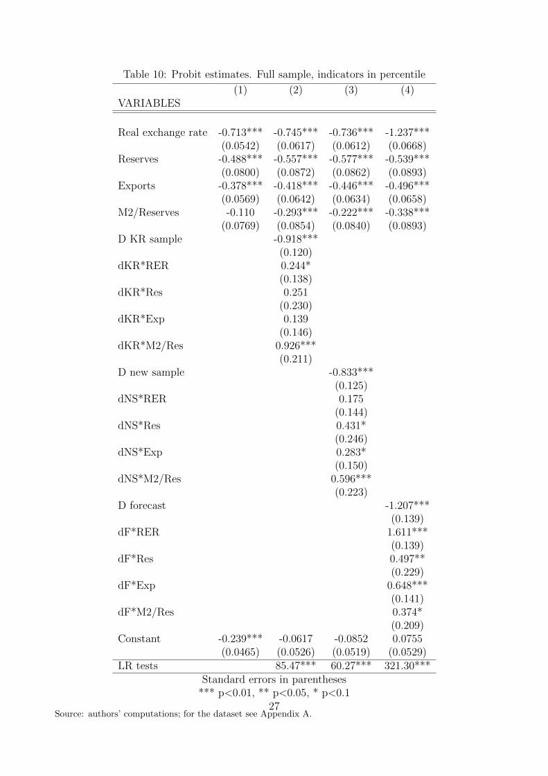
Table 11: Out-of-Sample Performance of the KLR EWI and the Pseudo-Financial EWI forthe 1997 Asian Crisis and the Great Recession (2006-2009) (signalling probability τ = 25; allmethods)

1997 Asian CrisisKLR BP Linear BP piecewise Probit KLR Sieve NLLS

KLR EWICorrectly called 78 68.99 64.60 66.67 72.73Sensitivity 32 25.78 18.62 51.57 22.64Specificity 87 83.12 76.54 71.46 88.621− P (C|S) 66 66.66 82.92 63.56 61.29QPS 0.26 0.34 0.37 0.26 0.38

Pseudo-Financial EWICorrectly called 84.11 69.23 66.14 75.15 65.15Sensitivity 7.42 28.87 18.30 25.79 28.93Specificity 99.31 82.56 76.44 90.82 76.651− P (C|S) 31.81 64.66 85.66 52.87 71.78QPS 0.27 0.36 0.36 0.34 0.36

Great Recession (2006-2009)KLR BP Linear BP piecewise Probit KLR Sieve NLLS

KLR EWICorrectly called 69 75.12 72.96 74.46 75.79Sensitivity 8 10.81 8.11 4.99 11.44Specificity 84 91.82 89.79 90.56 90.691− P (C|S) 88 74.47 82.91 89.10 77.84QPS 0.33 0.37 0.37 0.33 0.37

Pseudo-Financial EWICorrectly called 80.30 79.91 74.29 81.19 77.61Sensitivity 1.17 5.80 6.70 0.00 8.50Specificity 98.64 95.87 88.85 100 93.611− P (C|S) 83.33 76.79 88.55 - 76.42QPS 0.32 0.31 0.33 0.32 0.37

28

sum, greater than one, of Sensitivity and Specificity. Sensitivity is comparatively low with

respect to the in-sample results, but still appreciable since a crisis is correctly anticipated on

average, across all the methods, with 30 per cent probability for the KLR EWI and 21 per

cent for the pseudo-financial EWI.

It ought to be noticed that for the Asian crisis, the KLR method performs best among all

techniques when using the original KLR EWI, while it worsens when considering the pseudo-

financial EWI. This is not surprising, since it uses only 4 variables that makes the mapping

from the composite indicator to the probability space more troublesome. Instead, when the

mapping is done through the probit specification (i.e. KLR Probit), the performance of the

pseudo-financial EWI is comparable with the other methods.

Overall the two EWIs have very similar performances, hence indicating that there is no big

gain when focusing on the core pseudo-financial variables. The only exception is the average

probability of anticipating a crisis, P (C|S), that reveals a better average performance of the

pseudo-financial indicator (31 per cent versus 40 per cent on average).

The same conclusions cannot be drawn when considering the out-of-sample performance

for the period of the Great Recession (2006-2009), as reported in the lower part of Table 11.

Although the probability of “correctly-called” periods does not drop, the sum of Sensitivity

and Specificity falls and is not always greater than one across all methods. There is a relevant

decrease also in probability of correctly signalling a crisis, P (C|S), for both indicators. The

pseudo-financial EWI with the Sieve NLLS method is the best performing indicator.

In conclusion, no large difference is detected and both indicators have become much less

reliable during the Great Recession. Hence, we interpret this result as evidence of the insta-

bility in the relationship between exchange rates and fundamentals in the latter period that

does not vanish when restricting the core of fundamentals to the pseudo-financial variables.

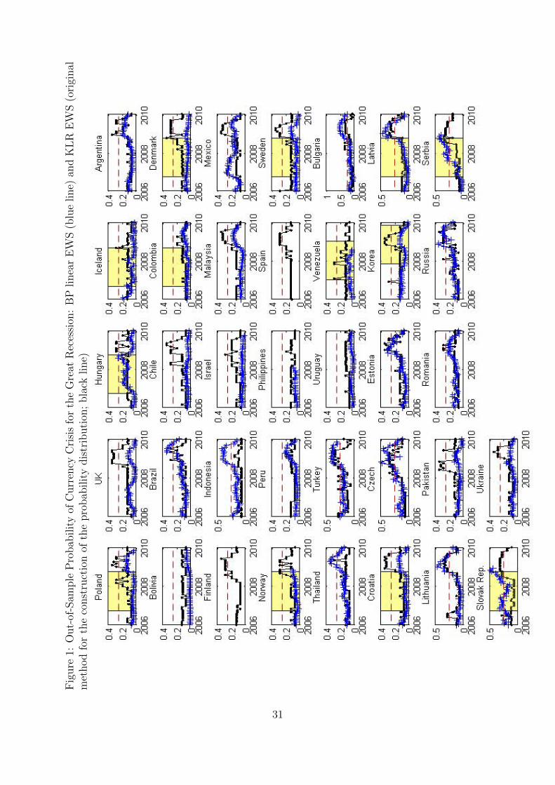
Finally, Figure 1 shows the out-of-sample conditional probabilities of all the currency crises

during the Great Recession for all the countries of our sample when using both the Sieve

NLLS and original KLR methods. We notice that the original KLR EWS correctly signals a

crisis only for seven countries (a signal inside the shaded area is issued for Poland, Hungary,

Venezuela, Korea, Serbia, Norway, Slovak Republic), while a false alarm is issued for all the

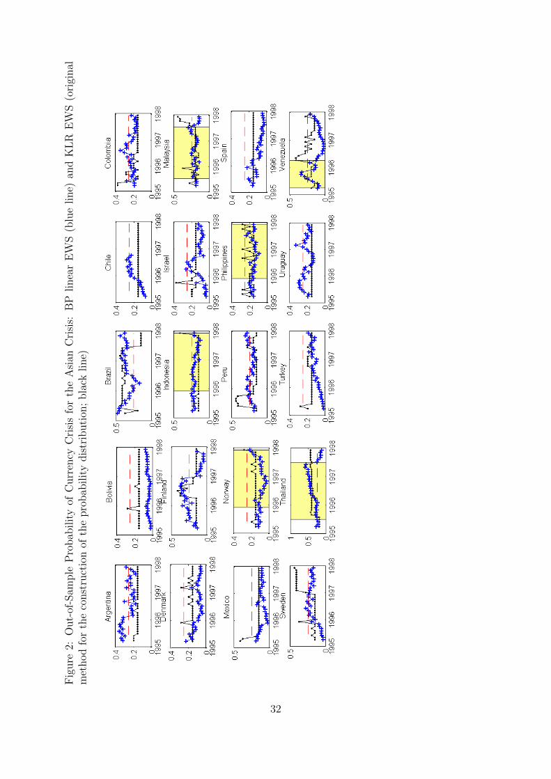
other countries. Figure 2 reports for comparison the same exercise for the Asian Crisis.

Figure 1 highlights the occurrence of a contemporaneous rise in probabilities of a crisis (that

is, a signal) in 32 countries (when considering both methods), although only 7 of them were

considered currency crises according to our definition. Such contemporaneous rise occurs in the

time span between the last quarter of 2008 and the first quarter of 2009, which corresponds to a

particularly bad period of the global financial crisis: Lehman Brothers collapsed in September

2008 and the world stock markets bottomed in March 2009.

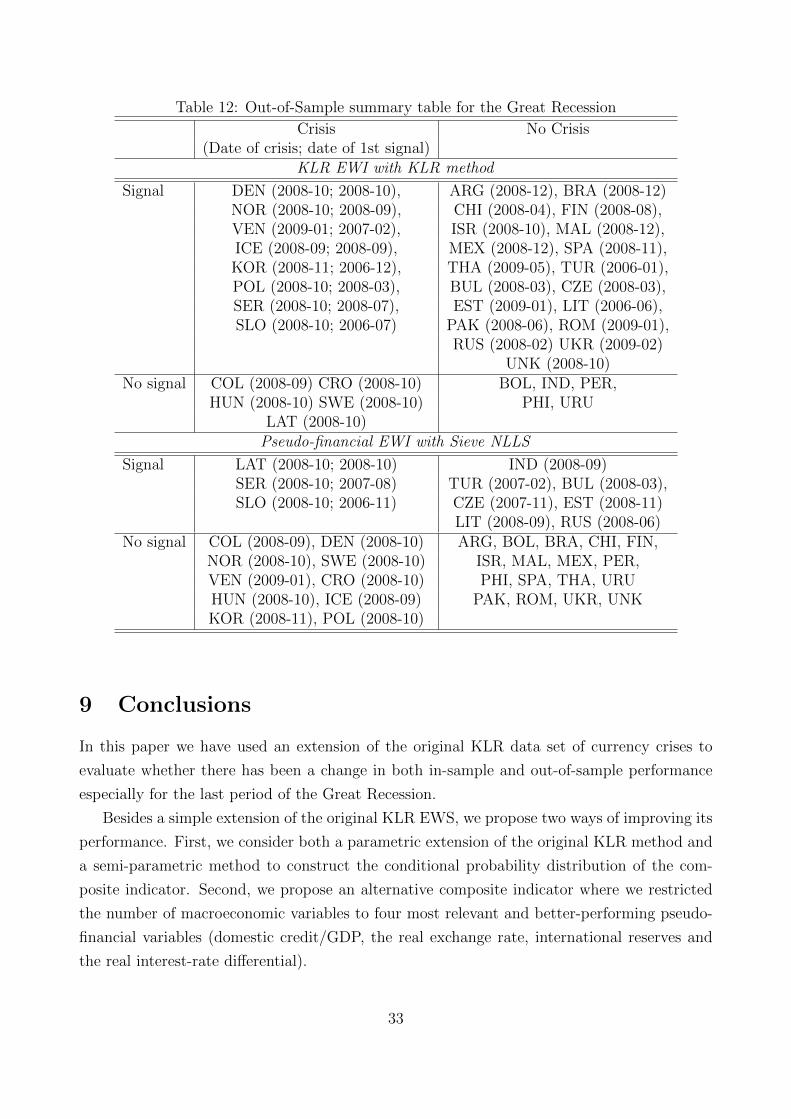
We summarize this qualitative result in Table 13, where we ordered countries according

29

to the out-of-sample indications coming from: (i) the KLR EWI and using the KLR method

to obtain the conditional probability of a crisis, (ii) the pseudo-financial EWI with the Sieve

NLLS method for the probability derivation. We choose these two methods coupled with

the relative EWIs because the Sieve NLLS is the best in the in-sample experiment and his

performance is good enough in out-of-sample forecast. KLR instead is a natural benchmark

in the EWS literature.12

The Sieve NLLS issues a good signal only for three crises, but it has the lowest number of

false alarms among all the methods. The group of countries that experienced a crisis but for

which no signal was issued had some relevant currency swings. This is a clear indication that

macroeconomic fundamentals have lost their predictive power in the latter period.

The KLR method instead is able to issue an early warning in Venezuela, Korea, Iceland,

Poland, Norway and a late warning for Denmark, Sweden and Croatia. Indeed, even if the

NLLS method is able to provide a better fit in aggregate13, KLR may be more interesting

from a qualitative point of view even though it is less reliable because of the high quantity of

false alarms.

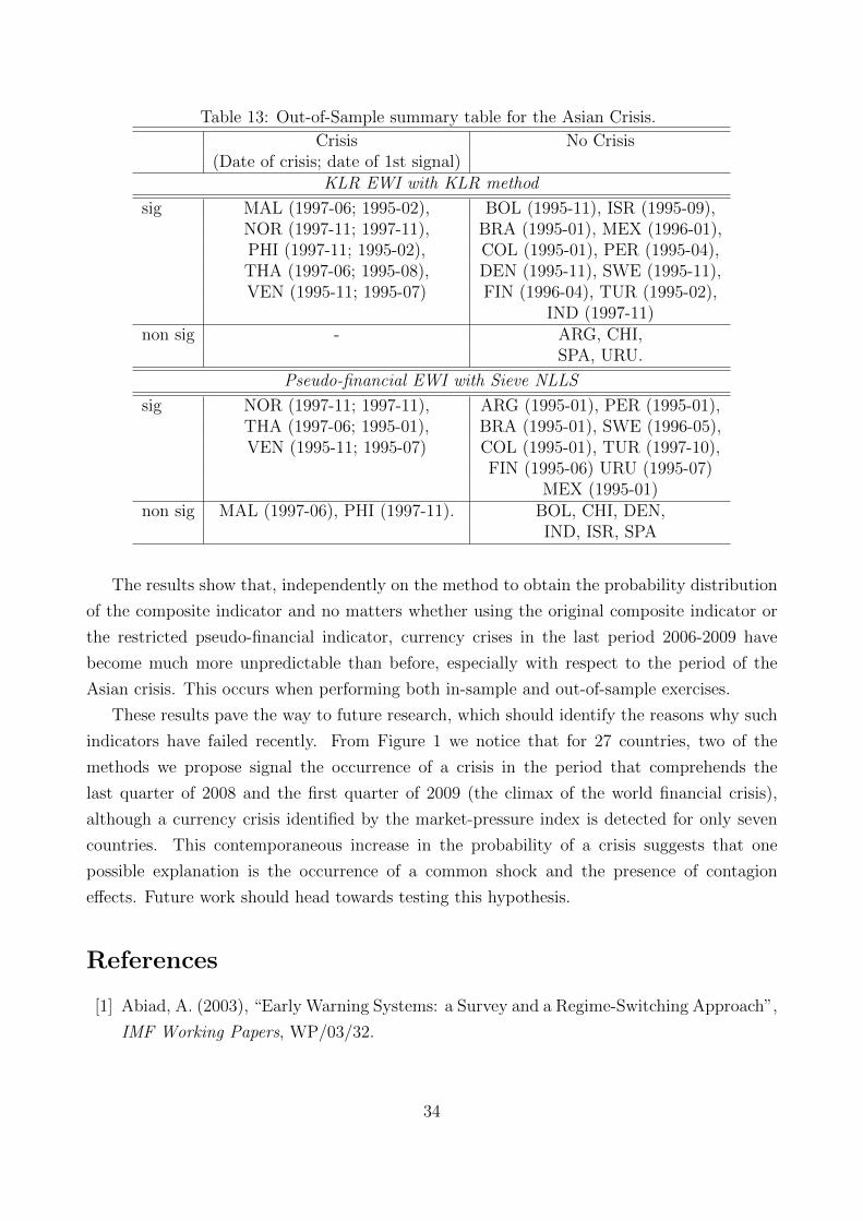
Regarding the performance of the two methods in forecasting the Asian crisis, a summary is

provided in table 12. As it has been noted before, KLR has the best out-of-sample performance;

as we can see from the table, it issued a signal for all the countries that had a crisis, though at

the cost of of a slightly higher number of false signals compared to other methods. However,

from a qualitative perspective, the two methods do not differ very much.

12Similar tables for all the other methods and EWIs are available upon request. In particular, in theliterature BP linear is the other traditional benchmark. NLLS performs better than BP linear because of lessfalse alarms and because it signals for a longer time when the signal is good. We should note however thatBP linear probit is qualitatively similar to Sieve NLLS.

13Our explanation for such a feature of the Sieve approach depends on the fact that it is smoother in thevariables and hence it produces a higher degree of autocorrelation of the fitted probabilities. So, when it issuesa good signal, usually it keeps signalling for a longer time, enhancing the sensitivity and thus boosting theoverall goodness of fit. Clearly this depends on the limitations of the classification table for binary variablesin a time-series context.

30

Fig

ure

1:O

ut-

of-S

ample

Pro

bab

ilit

yof

Curr

ency

Cri

sis

for

the

Gre

atR

eces

sion

:B

Plinea

rE

WS

(blu

eline)

and

KL

RE

WS

(ori

ginal

met

hod

for

the

const

ruct

ion

ofth

epro

bab

ilit

ydis

trib

uti

on;

bla

ckline)

31

Fig

ure

2:O

ut-

of-S

ample

Pro

bab

ilit

yof

Curr

ency

Cri

sis

for

the

Asi

anC

risi

s:B

Plinea

rE

WS

(blu

eline)

and

KL

RE

WS

(ori

ginal

met

hod

for

the

const

ruct

ion

ofth

epro

bab

ilit

ydis

trib

uti

on;

bla

ckline)

32

Table 12: Out-of-Sample summary table for the Great Recession

Crisis No Crisis(Date of crisis; date of 1st signal)

KLR EWI with KLR method

Signal DEN (2008-10; 2008-10), ARG (2008-12), BRA (2008-12)NOR (2008-10; 2008-09), CHI (2008-04), FIN (2008-08),VEN (2009-01; 2007-02), ISR (2008-10), MAL (2008-12),ICE (2008-09; 2008-09), MEX (2008-12), SPA (2008-11),KOR (2008-11; 2006-12), THA (2009-05), TUR (2006-01),POL (2008-10; 2008-03), BUL (2008-03), CZE (2008-03),SER (2008-10; 2008-07), EST (2009-01), LIT (2006-06),SLO (2008-10; 2006-07) PAK (2008-06), ROM (2009-01),

RUS (2008-02) UKR (2009-02)UNK (2008-10)

No signal COL (2008-09) CRO (2008-10) BOL, IND, PER,HUN (2008-10) SWE (2008-10) PHI, URU

LAT (2008-10)Pseudo-financial EWI with Sieve NLLS

Signal LAT (2008-10; 2008-10) IND (2008-09)SER (2008-10; 2007-08) TUR (2007-02), BUL (2008-03),SLO (2008-10; 2006-11) CZE (2007-11), EST (2008-11)

LIT (2008-09), RUS (2008-06)No signal COL (2008-09), DEN (2008-10) ARG, BOL, BRA, CHI, FIN,

NOR (2008-10), SWE (2008-10) ISR, MAL, MEX, PER,VEN (2009-01), CRO (2008-10) PHI, SPA, THA, URUHUN (2008-10), ICE (2008-09) PAK, ROM, UKR, UNKKOR (2008-11), POL (2008-10)

9 Conclusions

In this paper we have used an extension of the original KLR data set of currency crises to

evaluate whether there has been a change in both in-sample and out-of-sample performance

especially for the last period of the Great Recession.

Besides a simple extension of the original KLR EWS, we propose two ways of improving its

performance. First, we consider both a parametric extension of the original KLR method and

a semi-parametric method to construct the conditional probability distribution of the com-

posite indicator. Second, we propose an alternative composite indicator where we restricted

the number of macroeconomic variables to four most relevant and better-performing pseudo-

financial variables (domestic credit/GDP, the real exchange rate, international reserves and

the real interest-rate differential).

33

Table 13: Out-of-Sample summary table for the Asian Crisis.

Crisis No Crisis(Date of crisis; date of 1st signal)

KLR EWI with KLR method

sig MAL (1997-06; 1995-02), BOL (1995-11), ISR (1995-09),NOR (1997-11; 1997-11), BRA (1995-01), MEX (1996-01),PHI (1997-11; 1995-02), COL (1995-01), PER (1995-04),THA (1997-06; 1995-08), DEN (1995-11), SWE (1995-11),VEN (1995-11; 1995-07) FIN (1996-04), TUR (1995-02),

IND (1997-11)non sig - ARG, CHI,

SPA, URU.

Pseudo-financial EWI with Sieve NLLS

sig NOR (1997-11; 1997-11), ARG (1995-01), PER (1995-01),THA (1997-06; 1995-01), BRA (1995-01), SWE (1996-05),VEN (1995-11; 1995-07) COL (1995-01), TUR (1997-10),

FIN (1995-06) URU (1995-07)MEX (1995-01)

non sig MAL (1997-06), PHI (1997-11). BOL, CHI, DEN,IND, ISR, SPA

The results show that, independently on the method to obtain the probability distribution

of the composite indicator and no matters whether using the original composite indicator or

the restricted pseudo-financial indicator, currency crises in the last period 2006-2009 have

become much more unpredictable than before, especially with respect to the period of the

Asian crisis. This occurs when performing both in-sample and out-of-sample exercises.

These results pave the way to future research, which should identify the reasons why such

indicators have failed recently. From Figure 1 we notice that for 27 countries, two of the

methods we propose signal the occurrence of a crisis in the period that comprehends the

last quarter of 2008 and the first quarter of 2009 (the climax of the world financial crisis),

although a currency crisis identified by the market-pressure index is detected for only seven

countries. This contemporaneous increase in the probability of a crisis suggests that one

possible explanation is the occurrence of a common shock and the presence of contagion

effects. Future work should head towards testing this hypothesis.

References

[1] Abiad, A. (2003), “Early Warning Systems: a Survey and a Regime-Switching Approach”,

IMF Working Papers, WP/03/32.

34

[2] Anzuini, A. and G. Gandolfo (2003), “Can Currency Crises Be Forecast?”, in Gandolfo,

G. and F. Marzano (eds.) International Economic Flows, Currency Crises, Investment

and Economic Development: Essays in Memory of Vittorio Marrama, Roma, EUROMA

(Publications of the Faculty of Economics of the University of Rome La Sapienza), 2003,

pp. 61-82.

[3] Berg, A. and C. Patillo (1999), “Predicting Currency Crises: The Indicators Approach

and an Alternative”, Journal of International Money and Finance, vol. 18, pp. 561-86.

[4] Berg, A., Borensztein E. and C. Patillo (2005), “Assessing Early Warning Systems: How

Have They Worked in Practice?”, IMF Staff Papers, vol. 52(3), pages 5.

[5] Blevins, J. R. and S. Khan (2010), “Distribution-Free Estimation of Heteroskedastic

Binary Response Models in Stata”, mimeo.

[6] Chen, X. (2007). “Large Sample Sieve Estimation of Semi-Nonparametric Models”. In:

Heckman, J. J., Leamer, E. E. (Eds.), Handbook of Econometrics, vol. 6B. North-Holland,

Amsterdam.

[7] Edison, H. (2000), “Do Indicators of Financial Crises Work? An Evaluation of an Early

Warning System”, Board of Governors of the Federal Reserve System, International Fi-

nance Discussion Papers, n. 675.

[8] Frankel, J. and G. Saravelos (2010), “Are Leading Indicators of Financial Crises Useful

for Assessing Country Vulnerability? Evidence from the 2008-09 Global Crisis”, NBER

Working Paper n. 16047.

[9] Goldstein, M. and G. Kaminsky and C. Reinhart (2000), Assessing Financial Vulnera-

bility. An Early Warning System for Emerging Markets, Institute for International Eco-

nomics

[10] Horowitz, J. L. (1992), “A Smoothed Maximum Score Estimator for the Binary Response

Model”, Econometrica, 60, 505-531

[11] Kaminsky, G. and S. Lizondo and C. Reinhart (1998), “Leading Indicators of Currency

Crises”, IMF Staff Papers, 45, 48-64.

[12] Kaminsky, G. and C. Reinhart (1999), “The Twin Crises: Causes of Banking and Balance

of Payments Problems”, American Economic Review, vol. 89, Issue 3, pp. 473-500.

[13] Khan, S. (2010), “Distribution Free Estimation of Heteroskedastic Binary Response Mod-

els Using Probit/Logit Criterion Functions”, mimeo, Duke University

35

[14] Krugman, P. (1979), “A Model of Balance-of-Payments Crises”, Journal of Money, Credit

and Banking, vol. 11, Issue 3, pp. 311-25.

[15] Lane, P. and G. M. Milesi-Ferretti (2010), “The Cross Country Incidence of the

Global Crisis” mimeo prepared for the IMF/BOP/PSE Conference “Economic Linkages,

Spillovers and the Financial Crisis”, Paris, January 28-29 2010.

[16] Mansky, C. F. (1975), “Maximum Score Estimation of the Stochastic Utility Model of

Choice”, Journal of Econometrics, 3, 205-228

[17] Mansky, C. F. (1985), “Semiparametric Analysis of Discrete Response: Asymptotic Prop-

erties of Maximum Score Estimation”, Journal of Econometrics, 27, 313-334

[18] Obstfeld, M. and K. Rogoff (2009), “Global Imbalances and the Financial Crisis: Product

of Common Causes”, mimeo prepared for the Federal Reserve Bank of San Francisco Asia

Economic Policy Conference, Santa Barbara, CA, October 18-20, 2009.

[19] Powell, J. (1994). “Estimation of semiparametric models”. In: Engle III, R.F., McFadden,

D.F. (Eds.), Handbook of Econometrics, vol. 4. North-Holland, Amsterdam.

[20] Rose, A. and M. Spiegel (2009), “The Causes and Consequences of the 2008 Crisis: Early

Warning”, NBER Working Paper n. 15357.

[21] Shi, J. and Y. Gao (2010), “A Study on KLR Financial Crisis Early-Warning Model”,

Frontiers of Economics in China, vol. 5(2), pp. 254-75.

36

APPENDIX

A Description of the Data

Sample period: January 1970–January 2010.

Selected Countries

Original KR Countries: Argentina, Bolivia, Brazil, Chili, Columbia, Denmark, Fin-

land, Indonesia, Israel, Malaysia, Mexico, Norway, Peru, Philippines, Spain, Sweden, Thai-

land, Turkey, Uruguay, Venezuela.

New Added Countries (whole sample period unless indicated): Bulgaria (1990-), Croa-

tia, Czech Republic (1990-), Estonia (1990-), Hungary (1990-), Iceland, South Korea, Latvia

(1990-), Lithuania (1990-), Pakistan, Poland (1990-), Romania (1990-), Russia (1990-), Slovak

Republic (1990-), Ukraine, United Kingdom.

Macroeconomic Indicators

Indicators with the symbol * are 12-month percent change, otherwise they are in levels.

• M2 Multiplier*: M2/Base Money

• Domestic Credit/GDP*: Domestic Credit/GDP. Domestic credit is deflated using CPI.

Monthly GDP is obtained by linear interpolation of annual data.

• Real Interest Rate: rt = 1+it1+πt− 1, where it is the deposit rate and πt is the 12 month

CPI inflation rate.

• Lending/Deposit Rate Ratio: Lending rate/ deposit rate

• Excess M1 Balances : calculated for each country as the residual from a linear regression

of the type Mt/Pt = β0 + β1t+ β2Yt + β3it + ut, where t is a linear trend, Yt is monthly

real GDP (interpolated linearly) and it is the deposit rate.

• M2/Reserves Ratio*: M2/Reserves. M2 is converted in US dollars using monthly ex-

change rates.

• Bank Deposits*: Bank deposits are daflated using CPI

37

• Exports*

• Terms of Trade: unit value of exports/ unit value of imports

• Real Exchange Rate: since not all real appreciations are sympthoms of disequilibrium,

deviations from a linear trend are used as indicator.

• Imports*

• International Reserves*

• Real Interest Rate Differential : is the difference between real deposit rate in the domestic

country and the foreign country (US or Eurozone/Germany).

• Output*: monthly industrial production indices are used.

• Stock Prices*: stock indices.

• Deficit : cash surplus / nominal GDP. Monthly GDP and monthly deficits are obtained

by linear interpolation of annual data.

Data Sources

Most of the data are obtained from the online version of the International Financial Statis-

tics (IFS) of the IMF.

CPI: IFS line 64.

FX: national currency per US Dollars (end of period) IFS line AE.

RESERVES: Total reserves minus gold (USD). IFS line 1L.

M2: generally 59MB / Croatia, Philippines: IFS line 34 (Transferable deposits) + 35 (other

deposits).

BASE MONEY: IFS line 19MA or (Bulgaria, Finland, Korea, Latvia, Serbia) IFS line 14.

IPI: IFS line 66, IFS line 66aa index of output of primary commodities as alternative and

industrial employment index for Russia and Ukraine IFS line 67.

STOCK PRICES: IFS line 62 Share Price Index (end of period).

EXPORTS: IFS line 70. The unit of account changes depending on the country: Croa-

tia USD, Bulgaria Leva, Argentina USD, Bolivia USD, Brazil USD, Chile USD, Colombia

USD, Finland Markkaa/Euro, Indonesia USD, Norway Kroner, Malaysia Ringgit, Peru USD,

Phillipines Pesos, Sweden Kronor, Thailand Bath, Denmark Kroner, Czech Republic Koruny,

Estonia Kroony, Hungary Florint, Iceland Kronur, Korea USD, Latvia Lats, Lithuania Litai,

38

Pakistan Rupees, Poland Zloty, Romania USD, Russia USD, Serbia Dinars, Slovak Republic

Koruny/Euro, Ukraine USD, UK Pounds, Turkey USD, Venezuela Bolivares.

IMPORTS: IFS line 71 (unit-of-account currencies as for Exports).

TERMS OF TRADE: unit value of exports (IFS line 74) over unit value of imports (IFS

line 75).

LENDING RATE: 60P. Finland: line 60P until 2002M12. Average of lines 60pns, 60phm,

60phn, 60pcs. Poland spa: 60phm,pcs,pcn

DEPOSIT RATE: 60L England: Bank of England: Monthly average of Sterling certificates

of deposit interest rate, 3 months, mean offer/bid.

GDP: GDP at current prices line 99B. Monthly data obtained with linear interpolation.

GDP DEFLATOR: annual, 2005 = 100 line 99BIPZF.

DEFICIT: Cash Surplus/Deficit [1-2-31=1-2M] line CSD.

REER: generally IFS line RE (Real exchange rate index based on relative CPI). When it is

not available, we built a real exchange rate index (in base 2005=100) based on relative CPI

with the US, or with Germany for European countries.

M1: IFS line 59 (national definition) or line 34 (demand deposit).

B Dating the Crises

Table 14: Crisis dates according to different thresholds

Countries Fixed Moving threshold Rolling threshold Separate samples

(1970:1-1981:12 and 1982:1-2010:1)

Argentina Mar-75 Mar-75 Mar-75 Mar-75

Jun-75 Jun-75 Jun-75 Jun-75

Jul-82 Jul-82 Jul-82 Jul-82

Apr-89 Apr-89 Apr-89 Apr-89

Dic-89 Dic-89 Dic-89 Dic-89

Feb-90 Feb-90 Feb-90 Feb-90

- Mar-95 - -

- Jul-01 - -

- Jan-02 - Jan-02

- Feb-02 - Feb-02

- Mar-02 - Mar-02

- - - May-02

Continues on Next Page. . .

39

...continued

Countries Fixed Moving threshold Rolling threshold Two samples

- - - Jan-06

Bolivia Oct-72 Oct-72 Oct-72 Oct-72

- Nov-79 - -

Feb-82 Feb-82 Feb-82 Feb-82

Sep-85 Sep-85 Sep-85 Sep-85

- Feb-03 - Feb-03

- Oct-08 - Oct-08

Brazil - Jan-74 - -

Dic-79 Dic-79 Dic-79 Dic-79

Sep-82 Sep-82 Sep-82 Sep-82

Jan-83 - Jan-83 -

Feb-83 Feb-83 Feb-83 -

Mar-90 Mar-90 Mar-90 Mar-90

- Oct-97 - -

- Sep-98 Sep-98 -

Jan-99 Jan-99 Jan-99 Jan-99

Sep-02 - - -

- Sep-08 - -

Chile Jul-71 Jul-71 Jul-71 Jul-71

Sep-72 - - -

- Jun-82 - -

Jul-85 Jul-85 Jul-85 Jul-85

- Oct-95 - -

- Jun-99 - -

- Oct-08 - Oct-08

Colombia - - - Sep-74

- Jan-84 - -

- - Jan-85 -

- Aug-95 Aug-95 -

- Aug-07 Aug-07 -

Continues on Next Page. . .

40

...continued

Countries Fixed Moving threshold Rolling threshold Two samples

Sep-08 Sep-08 Sep-08 Sep-08

Denmark Oct-08 Oct-08 Oct-08 Oct-08

Finland - Jul-75 Jul-75 -

- - Nov-78 Nov-78

- - Oct-82 Oct-82

- - May-86 -

Mar-91 Mar-91 Mar-91 -

Sep-92 - Sep-92 Sep-92

Indonesia Nov-78 - Nov-78 Nov-78

- Mar-83 - Mar-83

- Apr-83 - Apr-83

Sep-86 Sep-86 Sep-86 Sep-86

- Aug-97 - -

- Oct-97 - -

- - Dic-97 -

Jan-98 Jan-98 Jan-98 Jan-98

May-98 - - -

Jun-98 - Jun-98 Jun-98

- Oct-08 - -

Israel Aug-71 Aug-71 Aug-71 Aug-71

Nov-74 Nov-74 Nov-74 Nov-74

Sep-75 - - -

Nov-77 Nov-77 Nov-77 Nov-77

- Aug-83 - -

- Oct-08 - Oct-08

Malaysia - Dic-92 - -

Jul-97 Jul-97 Jul-97 Jul-97

Aug-97 - Aug-97 Aug-97

Dic-97 - Dic-97 Dic-97

Continues on Next Page. . .

41

...continued

Countries Fixed Moving threshold Rolling threshold Two samples

Jan-98 Jan-98 Jan-98 Jan-98

- Oct-08 - -

Mexico Sep-76 Sep-76 Sep-76 Sep-76

Oct-76 - Oct-76 -

- Jun-81 - -

- Sep-81 - -

Feb-82 Feb-82 Feb-82 Feb-82

Dic-82 Dic-82 Dic-82 Dic-82

Dic-94 Dic-94 Dic-94 Dic-94

- - - Aug-98

- Oct-08 - Oct-08

Norway Nov-78 Nov-78 Nov-78 Nov-78

- - Jan-81 -

May-86 May-86 May-86 May-86

Mar-91 Mar-91 Mar-91 -

Nov-92 - Nov-92 Nov-92

Dic-97 Dic-97 Dic-97 Dic-97

Oct-08 Oct-08 Oct-08 Oct-08

Peru Jun-76 Jun-76 Jun-76 Jun-76

Oct-87 Oct-87 Oct-87 Oct-87

Dic-87 Dic-87 Dic-87 Dic-87

Sep-88 Sep-88 Sep-88 Sep-88

- Aug-05 - -

- - - Oct-08

Philippines Feb-70 Feb-70 Feb-70 Feb-70

- Jul-75 - -

- Jan-82 - -

- Nov-82 - -

- - Sep-83 -

Oct-83 Oct-83 Oct-83 Oct-83

Continues on Next Page. . .

42

...continued

Countries Fixed Moving threshold Rolling threshold Two samples

Jun-84 Jun-84 Jun-84 Jun-84

Feb-86 - - -

- Jul-97 - Jul-97

- Sep-97 - Sep-97

Dic-97 Dic-97 Dic-97 Dic-97

- - - Oct-00

- Oct-08 - -

Spain - Feb-76 Feb-76 -

- - Mar-80 -

- Mar-91 Mar-91 -

Sep-92 Sep-92 Sep-92 Sep-92

Oct-92 - Oct-92 -

Nov-92 - Nov-92 Nov-92

- Dic-98 - Dic-98

Sweden - Aug-77 Aug-77 Aug-77

Nov-92 Nov-92 Nov-92 Nov-92

Oct-08 Oct-08 Oct-08 Oct-08

Thailand - Nov-78 Nov-78 Nov-78

- Oct-79 Oct-79 -

- - Jul-81 Jul-81

- - - Feb-85

- - - Oct-85

- May-97 - -

- - - -

Jul-97 Jul-97 Jul-97 Jul-97

Aug-97 Aug-97 Aug-97 Aug-97

- - Nov-97 -

Dic-97 - Dic-97 Dic-97

Jan-98 - Jan-98 Jan-98

Turkey Aug-70 Aug-70 Aug-70 Aug-70

Continues on Next Page. . .

43

...continued

Countries Fixed Moving threshold Rolling threshold Two samples

- Oct-76 - -

Mar-78 Mar-78 Mar-78 -

Jan-80 - Jan-80 -

Feb-80 Feb-80 Feb-80 Feb-80

Feb-94 Feb-94 Feb-94 Feb-94

Mar-94 - Mar-94 Mar-94

Apr-94 Apr-94 Apr-94 Apr-94

- - - Feb-01

Mar-01 Mar-01 Mar-01 Mar-01

Apr-01 - - Apr-01

- Oct-08 - Oct-08

Uruguay Mar-72 Mar-72 Mar-72 Mar-72

Nov-82 Nov-82 Nov-82 Nov-82

Dic-82 Dic-82 Dic-82 Dic-82

- - - Nov-84

- Feb-02 - -

- - - Jun-02

Jul-02 Jul-02 Jul-02 Jul-02

- Sep-08 - -

Venezuela Feb-84 Feb-84 Feb-84 Feb-84

Dic-86 Dic-86 Dic-86 Dic-86

Mar-89 Mar-89 Mar-89 Mar-89

May-94 May-94 May-94 -

Dic-95 Dic-95 Dic-95 -

Apr-96 Apr-96 Apr-96 Apr-96

Feb-02 Feb-02 Feb-02 Feb-02

- Jan-03 - Jan-03

- Apr-07 - -

Jan-09 Jan-09 Jan-09 Jan-09

Bulgaria - - Jan-94 -

Jul-94 - - -

Continues on Next Page. . .

44

...continued

Countries Fixed Moving threshold Rolling threshold Two samples

- - - Jan-96

- - - Mar-96

- - - May-96

- - - Jul-96

- Oct-08 - -

Croatia - - Feb-95 -

Oct-08 Oct-08 Oct-08 Oct-08

Jan-09 Jan-09 Jan-09 Jan-09

Czech - - Feb-93 -

- Aug-08 - -

- Oct-08 - -

- Jan-09 - Jan-09

Estonia - - Jul-92 -

- - - Jan-09

Hungary - - Sep-89 -

Oct-08 Oct-08 Oct-08 Oct-08

Jan-09 Jan-09 Jan-09 Jan-09

Iceland - Dic-72 - -

Sep-74 Sep-74 Sep-74 Sep-74

Feb-75 Feb-75 Feb-75 Feb-75

Aug-82 Aug-82 Aug-82 Aug-82

May-83 May-83 May-83 May-83

Sep-08 - Sep-08 Sep-08

Oct-08 - Oct-08 Oct-08

Korea - Jun-71 - -

- Dic-71 - -

Jan-80 Jan-80 Jan-80 Jan-80

Nov-97 Nov-97 Nov-97 Nov-97

Continues on Next Page. . .

45

...continued

Countries Fixed Moving threshold Rolling threshold Two samples

Dic-97 Dic-97 Dic-97 Dic-97

- Sep-08 - -

Nov-08 Nov-08 Nov-08 -

Latvia - - Feb-94 -

Oct-08 Oct-08 Oct-08 Oct-08

- - Nov-08 -

Jan-09 - Jan-09 Jan-09

Lithuania - - Jan-93 -

Pakistan May-72 May-72 May-72 May-72

- - - Oct-96

- Mar-08 - -

- May-08 - -

- Aug-08 - -

Poland Jul-86 - Jul-86 -

May-89 - - May-89

- Mar-05 - -

Oct-08 Oct-08 Oct-08 Oct-08

Jan-09 - Jan-09 Jan-09

Romania - - Feb-79 -

May-89 May-89 May-89 -

Aug-89 Aug-89 Aug-89 Aug-89

Feb-90 - Feb-90 Feb-90

Nov-90 - Nov-90 Nov-90

- Jan-97 - Jan-97

- - - Feb-97

- - - Nov-99

- Oct-08 - -

- Jan-09 - -

Continues on Next Page. . .

46

...continued

Countries Fixed Moving threshold Rolling threshold Two samples

Russia - - Jul-96 -

Aug-98 - Aug-98 Aug-98

Sep-98 Sep-98 Sep-98 Sep-98

- Oct-08 - -

- Jan-09 - -

Serbia - - Jan-02 -

Oct-08 Oct-08 Oct-08 Oct-08

Jan-09 - Jan-09 Jan-09

Slovak Rep. - - Feb-93 -

Oct-08 Oct-08 Oct-08 Oct-08

Ukraine - - Jan-93 -

Mar-93 - - -

Dic-93 - - -

Jun-94 Jun-94 Jun-94 Jun-94

Oct-94 - - -

- - - Sep-98

- Oct-08 - Oct-08

- Nov-08 - Nov-08

- Dic-08 - -

UK - Jul-72 Jul-72 -

Sep-92 - - Sep-92

Oct-92 - - Oct-92

- Jan-97 - Jan-97

- Aug-08 - Aug-08

- Oct-08 - Oct-08

47