Petroleum Retailing, Station Level Demand and the Retail Price Cycles Submitted by Murat Besnek B.Ec (Hons1) La Trobe University 2005 A thesis submitted in total fulfilment of the requirements for the degree of Doctor of Philosophy (Economics) At School of Economics Faculty of Law and Management La Trobe University Bundoora, Victoria 3086 Australia November 2012
Transcript
Petroleum Retailing, Station Level Demand and the Retail Price Cycles
Submitted by
Murat Besnek B.Ec (Hons1) La Trobe University 2005
A thesis submitted in total fulfilment of the requirements for the degree of
Doctor of Philosophy
(Economics)
At
School of Economics Faculty of Law and Management
La Trobe University
Bundoora, Victoria 3086 Australia
November 2012
ii
Dedicated to my father, Fuat, and my mentor, Said Nursi.
prices of petrol cycle. Interestingly, thus far, there has been no definite answer.
In theory, there are many reasons why retail prices may cycle in a market: competition, consumer
acquisition and price discrimination to list a few (Maskin & Tirole 1988; Doyle 1983; Conlisk et al.
1984). The conclusions of preceding papers, except for Foros and Steen (2008), are that retail prices
of petrol cycle because of competition that exists between service stations. They claim that the
cycles are explained by the Edgeworth cycles model in Maskin and Tirole (1988). For instance, Noel
(2007: 81-87) believes that it is the constant tug of war between small and large firms that generate
the cycling phenomenon. BP Australia (2006: 3) claims that “the price cycles reflect competition in
the market.” Australian Competition and Consumer Commission (ACCC 2007: 167) reports that “the
causes of the price cycles are not clear” and that “the existence of price cycles alone do not seem to
provide evidence of a lack of retail competition.”
In this dissertation, using (1) our experience as a service station operator and worker for more than
three years in five sites; (2) meetings with an owner of a company that manages more than thirty
service stations; (3) interviews from four service station operators; and (4) micro-level price and
quantity data1, we propose that retail prices of petrol do not cycle because of competition that exists
between service stations. We present the first piece of empirical evidence against the common
1 We acquire the data from the print-outs of the on-site computer systems of four service stations, which we
personally print out and enter into a spreadsheet. From the time we were given permission to retrieve the data to its current state which is ready for estimation, took approximately six months.
2
belief that the Edgeworth cycles model is consistent with the retail petrol industry. The similar price
elasticity estimates, recurring cycle lengths, price matching, and limited variation in the sales of
service stations that we establish from the data oppose the idea that competition is the cause of the
cycles. If competition is the cause of the cycles, then a new theory other than the Edgeworth cycles
model should be proposed.
In Chapter 2 of this dissertation, we explain how petrol, diesel and LPG are retailed in Australia. The
purpose is to shed light on to retail petroleum industry to assist with the analysis regarding the
cause of the cycles in Chapter 4. We provide information about each level of the petroleum industry,
discuss consumer and service station decision making, and examine when service stations change
their prices and how this affects their sales. We find cycles that do not vary in length, steady sales
levels at service stations, price matching rather than price cutting between service stations, the LPG
market displaying cycles and different pricing patterns in markets without cycles. There are several
details concerning the retail petroleum industry presented in this chapter that are not consistent
with the Edgeworth cycles model.
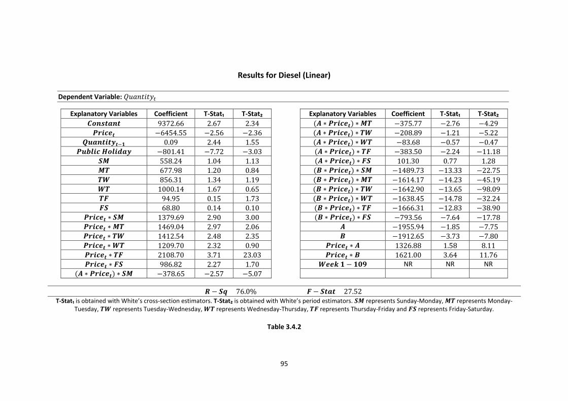
In Chapter 3 of this dissertation, we provide station level demand estimates for diesel and LPG in
four service stations that operate in metropolitan Melbourne. The purpose is to offer some insight
into how elastic or inelastic demand for diesel or LPG is in Australia. The estimates predict that the
short-run price elasticities of diesel are between to and of LPG between to
. To our knowledge, there is no previous Australian study that has estimated demand for
diesel or LPG. The estimates in this chapter not only serve as good comparisons to the petrol
estimates in Chapter 4 which will assist in determining the cause of the cycles, but also offer policy
makers in Australia a measure to judge if the ongoing tax raises on LPG will have significant effects
on the sales of service stations.
In Chapter 4 of this dissertation, we identify differences in the predictions of the Edgeworth cycles
model (Maskin & Tirole 1988) and the price discrimination model (Conlisk et al. 1984) that can be
3
empirically analysed. The purpose is to present the first piece of empirical evidence to reject the
prediction that there are price differences across service stations. The Edgeworth cycles model and
the current explanations for the cycles in petrol retailing predict price differences across service
stations. However, to date, there has been no empirical evidence in the literature to support this
prediction. By estimating station level demand for petrol in four service stations that operate in
Metropolitan Melbourne, we show that the similar price elasticities in local markets that have
different levels of competition indicate that service stations match each other’s prices and not
undercut. Therefore, (1) suggesting that the cycles are not in line with the Edgeworth cycles model
and (2) associating the cycles with other motives like price discrimination.
4
Bibliography
Atkinson, B. (2009) Retail Gasoline Price Cycles: Evidence from Guelph, Ontario Using Bi-Hourly,
Station Specific Retail Price Date. The Energy Journal. 30(1): 85-109.
Australian Competition and Consumer Commission (ACCC) (2000) Report on the Movement in Fuel
Prices in the September Quarter 2000. Canberra: ACCC.
Conlisk, J., Gerstner, E. and Sobel, J. (1984) Cyclic Pricing by a Durable Goods Monopolist. The
Quarter Journal of Economics. 99(3): 489-505.
Doyle, C. (1983) Dynamic Price Discrimination, Competitive Markets and the Matching Process.
Discussion Paper 229, University of Warwick.
5
Doyle, J., Muehlegger, E. and Samphantharak, K. (2008) Edgeworth Cycles Revisited. NBER Working
Paper 14162.
Eckert, A. (2002) Retail Price Cycles and Response Asymmetry. Canadian Journal of Economics. 35(1):
52-77.
Eckert, A. (2003) Retail Price Cycles and Presence of Small Firms. International Journal of Industrial
Organization. 21(2): 151-170.
Eckert, A. and West, D. (2004) Retail Gasoline Price Cycles across Spatially Dispersed Gasoline
Stations. Journal of Law and Economics. 22: 997-1015.
Foros, O. and Steen, F. (2008) Gasoline Prices Jump Up on Mondays: an Outcome of Aggressive
Competition? CEPR Working Paper DP6783.
Lewis, M. (2009) Temporary Wholesale Gasoline Price Spikes have Long Lasting Retail Effects: The
Aftermath of Hurricane Rita. Journal of Law and Economics. 52(3): 581-606.
Lewis, M. and Noel, M. (2011) The Speed of Gasoline Price Response in Markets with and without
Edgeworth Cycles. Review of Economics and Statistics. 93(2): 672-682.
Maskin, E. and Tirole, J. (1988) A Theory of Dynamic Oligopoly II: Price Competition, Kinked Demand
Curves and Edgeworth Cycles. Econometrica. 56(3): 571-599.
Noel, Michael D. (2007) Edgeworth Price Cycles: Evidence from the Toronto Retail Gasoline Market.
Journal of Industrial Economics. 55(1): 69-92.
——(2011) Edgeworth Price Cycles and Intertemporal Price Discrimination. Energy Economics.
Forthcoming.
Wang, Z. (2009a) Station Level Gasoline (Petrol) Demand in an Australian Market with Regular Price
Cycles. Australian Journal of Agricultural and Resource Economics. 53(4): 467-483.
Wang, Z. (2009b) Mixed Strategies in Oligopoly Pricing: Evidence from Gasoline Price Cycles before
and under a Timing Regulation. Journal of Political Economy. 117(6): 987-1030.
6
2. Retailing of Petrol, Diesel and LPG in Australia
2.1 Introduction
In recent times, the retail petroleum industry has received the attention of academics (Atkinson
2009; Bloch 2010; Doyle 2008; Eckert 2002, 2003; Eckert & West 2004; Foros & Steen 2008; Lewis
2009; Lewis & Noel 2011; Noel 2007, 2011; Wang 2009a, 2009b) and regulatory authorities (ACCC
2000, 2001a, 2001b, 2004, 2005, 2006, 2007, 2010a, 2010b) because of the price cycles that occur in
petrol retailing. As petrol is a vital consumer good and forms a big portion of household expenditure,
this attention is quite understandable. Yet, the regular and predictable cycles are actually eye-
catching themselves. In Melbourne 20062, a typical cycle begins on a Wednesday afternoon with a
single large increase in price, approximately cents per litre on average. Thereafter, prices steadily
fall for six days, several small decreases of about cent per litre on average. This is until the
following Wednesday afternoon, whereupon the price is raised again and a new cycle begins.
Preceding academic and regulatory papers, even the ones explaining the retail petroleum industry of
other countries, are written from the perspective of an outsider looking into the industry. None of
the writers ever speak about working or operating a service station. Furthermore, nearly all
preceding academic papers either use macro-level data or micro-level data that only contains price
observations. The only paper that uses micro-level price and quantity data is Wang (2009a).
Unfortunately, however, the data in Wang (2009a) is collected at a time when the retail market in
Western Australia is under severe restrictions by the regulatory authorities and service stations are
not allowed to change their prices to match or beat their competitors' prices. As a result, the
descriptions in Wang (2009a) are less relevant outside Western Australia.
We believe having inside information and micro-level price and quantity data collected under regular
conditions where service stations are allowed to change their prices as many times as they desire is
2 During other periods or in other cities prices may cycle on a different day.
7
critical in being able to explain the retail petroleum industry. In this chapter, we explain how petrol,
diesel and LPG are retailed in Australia using (1) our experience as a service station operator and
worker for more than three years in five sites; (2) meetings with an owner of a company that
manages more than thirty service stations; (3) interviews from four service station operators; and (4)
micro-level price and quantity data. Moreover, we investigate when service stations change their
prices and how this affects their sales. The aim in undertaking this study is to improve the overall
understanding of the industry so that future research dealing with questions like ‘why does retail
prices of petrol cycle?’ can make the right decisions when choosing the assumptions of their models
and interpreting industry data.
This chapter is organised as follows. Section 2.2 outlines the data and provides details about the
service stations from where the data is acquired. Section 2.3 explains the Australian petroleum
industry. Section 2.4 provides information about consumer and service station decision making.
Sections 2.5, 2.6 and 2.7 examine the retail petrol, diesel and LPG markets to determine when
service stations change their prices and how this affects their sales. Section 2.8 concludes the
chapter.
2.2 Dataset and Service Stations
2.2.1 Dataset
The dataset we use is made up of intraday observations on retail prices and quantities sold of petrol,
diesel and LPG during the years of 2004, 2005 and 2006. We acquire the data from four service
stations located within the Melbourne metropolitan area and surrounding suburbs. Due to a
confidentiality agreement with the operators, we do not disclose their position and brand name. We
have labelled them (A), (B), (C) and (D) to allow fluency when writing. The letters chosen are random
8
and do not represent anything. All of the service stations are branded independents3 and they
compete in separate local markets.
We compile the observations directly from the on-site computer systems of the service stations,
which on a daily basis—24 hour period to 3pm—report the volume of sales in litres at the registered
prices of petrol, diesel and LPG. For instance, at 3pm on the 23rd of April 2006, the computer system
of one of the service stations reports the sale of litres of petrol at the price of dollars
per litre and litres of petrol at the price of dollars per litre. This sales report accounts
for all petrol sold from that particular service station between 3pm on the 22nd of April 2006 and
3pm on the 23rd of April 2006. The prices are reported in order of registration; however, the time of
registration is not made known. In other words, the computer system of that particular service
station reports that petrol is firstly sold for dollars per litre and later for dollars per litre.
It does not however report the exact time the price change occurs and as a result we do not know
the time-span of each registered price.
Petrol refers to unleaded fuel with a minimum Research Octane Number (RON) of 91. Octane
numbers indicate the quality of fuel; higher octane fuels undergo longer manufacturing processes at
the oil refinery. Higher octane fuels are required by high performance vehicles; hence,
predominantly used by them. We do not include unleaded fuel other than 91 octane in the dataset
for two reasons. Firstly, about of unleaded fuel sold in the service stations is 91 octane
unleaded. Secondly, the prices of other unleaded fuels move precisely in the same manner as 91
octane unleaded. In Australia, service stations retail higher octane fuels at a constant mark-up over
the prices of 91 octane unleaded. For instance, 95 octane unleaded always sells seven cents above
91 octane unleaded during the period of the data.
3 A branded independent service station is a service station operated independently of the oil majors, but is
branded with one of their names. For further details see section 2.3.3 on p.21.
9
The dataset also includes the average daily terminal gate price (TGP)4 of petrol and diesel for the
years of 2004, 2005 and 2006. We could not acquire any data on the TGP of LPG. We obtain the
average daily TGP of petrol and diesel from the Australian Institute of Petroleum (AIP) website
(www.aip.com.au). It is prepared by ORIMA Research Pty Ltd and runs from the 1st of January 2004
to the present day. ORIMA reports that the TGP is calculated from information provided on the
websites of the four oil majors. ExxonMobil, Royal Dutch Shell, BP and Chevron5 publish their TGP on
the internet on a daily basis. ORIMA every morning collates the average TGP of these companies for
the day and records it. Prices are inclusive of GST.
2.2.2 Pricing strategy of the owner of the service stations
The owner of the four service stations where we acquire the data from also manages more than
thirty other service stations in Melbourne. The owner entered into the retail petroleum industry
many years ago by purchasing a single service station and operating as an independent before
purchasing additional service stations. At present, his service stations are branded independents.
Naturally, as the owner purchased more and more service stations, he was compelled to manage
rather than operate. The owner currently employs individuals on monthly contracts to operate his
service stations while he manages. A standard contract includes the following terms:
1. The operator to agree to pay the owner a sum of money for having the right to operate a
service station for a given month.
2. To operate a service station, the operator to invest in stock made up of items that the oil
major they are branded with has approved of, varying from to dollars,
depending on the size of the service station.
3. The operator to use these items to stock up the service station he operates, as the owner is
only responsible in providing fuel.
4 The TGP broadly represents the price for bulk supply of petroleum excluding charges for additional services
such as freight to the retail outlet. For further details see section 2.3.1 on p.16. 5 In Australia, Chevron is represented by its subsidiary Caltex.
10
4. The operator to receive cent per litre from fuel sales at the service station he operates6.
5. The operator to receive the profits earned from the sale of non-fuel items excluding the car
wash (if applicable).
6. The owner to pay the water, gas and electricity bills.
The owner demands that his service station operators match the lowest price in the local markets
they operate in. He gives them strict orders. The owner truly believes that this strategy maximises
his profits and openly states that he has adopted other strategies beforehand, such as undercutting
the available market price, but these have lead to lower profits. There are three ways in which the
operators try to match the lowest price in the local markets they operate in. We will summarise each
in turn.
The first way in which the operators try to match the lowest price in the local markets they operate
in is by ordering employees to inspect the prices of competing service stations either visually if they
are in close vicinity or through shift changes if they are distant. If the prices of competing service
stations are lower, the operators authorise a price change immediately by ringing the owner. Once a
price change has been authorised, the new price is keyed into the register and changed on the price
board. There are commonly three or four shift changes during a 24 hour period, so if competing
service stations are distant, inspecting prices through shift changes is an effective way that operators
can match the lowest price in the local markets they operate in.
The second way in which the operators try to match the lowest price in the local markets they
operate in is by utilising the recommended price they receive on a daily basis from the oil major they
are branded with. This price generally serves as a good estimate for the lowest price in the local
markets they operate in. If their current price is significantly higher or lower than this recommended
6 The operators receive the cent per litre irrespective of the price or cost of fuel. Even if the owner sells
below cost, the operators still receive the cent per litre.
11
price, the operators immediately order employees to re-inspect the prices of competing service
stations.
The third way in which the operators try to match the lowest price in the local markets they operate
in is by communicating with the owner. The owner is in a position to continually update the
operators as he is aware of the prices of many service stations that are spread all over Melbourne.
Just like the daily recommended price, the operators make use of this information by comparing
their current price to the prices of other service stations. If something appears to be a little odd, the
operators immediately order employees to re-inspect the prices of competing service stations.
2.2.3 Service stations7
Figure 2.1.1 below displays the market structure of service station (A)8. Service station (A) competes
with three independent service stations9 denoted as (I), which lie 250m to the east. The three
independent service stations lie directly across each other; hence, are approximately equivalent in
distance from where service station (A) is located. The prices of the three independent service
stations are visible from where service station (A) is located. The operator or any employee can walk
to the entrance of the site and identify what prices the independent service stations have set. It can
be said with confidence that service station (A) is at all times matching the lowest price in its local
market.
7 Information about which service stations compete with service stations (A), (B), (C) and (D) are provided by
the operators. 8 The arrows in the figures report the distance between the service stations.
9 An independent service station is a service station operated independently of the oil majors. For further
details see section 2.3.3 on p.21.
12
Market Structure of Service Station (A)
Figure 2.1.1
Service station (A) and the top two independent service stations compete for market share when
motor vehicles are travelling east on a major road that runs from where service station (A) is
positioned. The top and bottom independent service stations furthest to the right compete for
market share when motor vehicles are travelling south on a different major road that runs from
where the top independent service station is positioned. There are traffic lights at the intersection of
these two major roads; thus, motor vehicles travelling one way can change direction if there are
price differences across the service stations.
Figure 2.1.2 below displays the market structure of service station (B). Service station (B) competes
with one supermarket operated service station10 denoted as (S) and three oil major11/branded
independent service stations denoted as (OM/BI). The three oil major/branded independent service
stations are labelled (OM/BI) because it is not definite if they are oil major franchisees or branded
independents. From the exterior they both look identical; without any details on how the service
stations are operated, their ownership is not identifiable. Service station (B) in contrast to service
station (A) is isolated from its competitors. The nearest service station lies 5.2km to the west. Service
station (B) monitors the prices of competing service stations through shift changes for the reason
10
A supermarket operated service station is a service station operated by one of the supermarket chains. For further details see section 2.3.3 on p.21. 11
An oil major service station is a service station operated by one of the oil majors. For further details see section 2.3.3 on p.21.
13
that it is so distant from where its competitors lie. The operator of service station (B) also receives
considerable help from the owner, who informs him of any updates received from the oil major or
other operators. The operator of service station (B) states that even if they are not able to match
their competitors’ prices instantly because of their location, they are quick to respond. He openly
claims that the loss of consumers from the delay is insignificant.
Market Structure of Service Station (B)
Figure 2.1.2
The top oil major/branded independent service station and the supermarket operated service
station compete for market share when motor vehicles are travelling east on a major road that runs
from where the top oil major/branded independent service station is positioned. The middle and
bottom oil major/branded independent service stations compete for market share when motor
vehicles are travelling west on the same major road. Service station (B), because of its position,
competes with all four service stations; motor vehicles travelling east or west are able to enter it
without changing direction. To access the bottom oil major/branded independent service station,
motor vehicles have to make a left turn when travelling west and drive a further 400m. There are
many traffic lights along this major road; therefore, motor vehicles travelling one way can change
direction if there are price differences across the service stations. Furthermore, this major road is
not a freeway and contains speed limits and traffic volumes comparable to the two major roads in
the local market of service station (A).
14
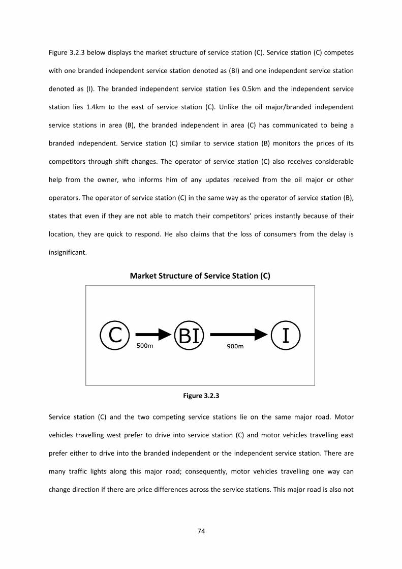
Figure 2.1.3 below displays the market structure of service station (C). Service station (C) competes
with one branded independent service station denoted as (BI) and one independent service station
denoted as (I). The branded independent service station lies 0.5km and the independent service
station lies 1.4km to the east of service station (C). Unlike the oil major/branded independent
service stations in area (B), the branded independent in area (C) has communicated to being a
branded independent. Service station (C) similar to service station (B) monitors the prices of its
competitors through shift changes. The operator of service station (C) also receives considerable
help from the owner, who informs him of any updates received from the oil major or other
operators. The operator of service station (C) in the same way as the operator of service station (B),
states that even if they are not able to match their competitors’ prices instantly because of their
location, they are quick to respond. He also claims that the loss of consumers from the delay is
insignificant.
Market Structure of Service Station (C)
Figure 2.1.3
Service station (C) and the two competing service stations lie on the same major road. Motor
vehicles travelling west prefer to drive into service station (C) and motor vehicles travelling east
prefer either to drive into the branded independent or the independent service station. There are
many traffic lights along this major road; consequently, motor vehicles travelling one way can
change direction if there are price differences across the service stations. This major road is also not
15
a freeway but contains lower speed limits and higher traffic volumes than the major roads in the
local markets of service stations (A) and (B).
Figure 2.1.4 below displays the market structure of service station (D). Service station (D) competes
with one independent service station denoted as (I), one branded independent service station
denoted as (BI), and one supermarket operated service station denoted as (S). The independent
service station lies directly across service station (D), practically facing one another. The branded
independent service station lies 600 metres to the east and the supermarket operated service
station lies 800 metres to the west of service station (D). Service station (D) monitors the prices of its
competitors in a unique way. Like service station (A), it can directly observe the price of the
independent service station. It is also aware of the price at the branded independent service station
because it is one of the other service stations the owner has purchased. Only the price of the
supermarket operated service station needs to be monitored and because service station (D) is a
large site, it has two employees working at all times making monitoring more frequent than in
service stations (B) or (C). For this reason, it can be said with confidence that just like service station
(A), service station (D) is at all times matching the lowest price in its local market.
Market Structure of Service Station (D)
Figure 2.1.4
Service station (D) and the three competing service stations lie on the same major road. Motor
vehicles travelling west prefer to drive into the branded independent service station and motor
vehicles travelling east prefer either to drive into the supermarket operated service station, the
16
independent service station or service station (D). There are many traffic lights along this major
road; consequently, motor vehicles travelling one way can change direction if there are price
differences across the service stations. This major road is also not a freeway and contains speed
limits and traffic volumes comparable to the major roads in the local markets of service stations (A)
and (B).
2.3 Australian Petroleum Industry
2.3.1 Refining
The Australian petroleum industry can be classified into three broad levels: refining, distributing and
retailing. Refining petroleum refers to the process of separating crude oil and natural gas into
different fractions by distillation (AIP Refining of Petroleum n.d.). Crude oil and natural gas are of
little use when extracted from the ground in their natural state. Refineries organise a series of
processes that remove and group elements from crude oil and natural gas to transform them into
products like petrol, diesel and LPG. There are seven refineries operating in Australia with one at
Port Stanvac in South Australia12 stopping production. They are all operated by the oil majors:
ExxonMobil, Royal Dutch Shell, BP and Chevron own two refineries each. The refineries are fairly
evenly spread across the main states of Australia. There are two refineries in Victoria, one in Altona
operated by ExxonMobil and one in Geelong operated by Royal Dutch Shell. New South Wales has
two refineries, one in Kurnell operated by Chevron and one in Clyde operated by Royal Dutch Shell.
Queensland has two refineries, one in Bulwer Island operated by BP and one in Lytton operated by
Chevron. Western Australia has one refinery in Kwinana operated by BP.
The annual capacity of the seven refineries was million litres in 2009-10 (ACCC 2010a).
However, there has been a decline in refining capacity since 2003 when the annual capacity was
million litres (ACCC 2006). This decline is mainly due to the fact that the Port Stanvac refinery
12
One of ExxonMobil’s refineries.
17
ceased to operate and the re-configuration of the other refineries to meet the new cleaner fuel
standards introduced in 2002. The higher average cost of refining in Port Stanvac because of its
relative size compared to the larger refineries in the Asia-Pacific region is the reason why it ceased to
operate. The introduction of the new cleaner fuel standards in 2002 is an initiative by the Australian
Government to reduce global warming and pollution in general (ACCC 2006). The standards simply
limit the use of certain chemicals in petroleum products. Other notable impacts of the introduction
of the new cleaner fuel standards are cents per litre increase in the retail prices of fuel and the
effect on independent importers who now find it more difficult to obtain fuel that meet the new
cleaner fuel standards (ACCC 2006).
It would be an understatement to say that the oil majors completely dominate the refinery level.
They own the refineries and the independent importers source most of their fuel from them. For
example, in 2009-10 the seven refineries collectively produced million litres of petrol (ACCC
2010a). Motorists consumed million litres in the same year and there were litres of
petrol imported. The discrepancy between production/imports and consumption is due to the
existence of stocks. Imports make up of total consumption of petrol, a fairly small share. More
importantly, however, most of the importing of petrol is carried out by the oil majors to meet
demand in areas that are distant from their refineries (ACCC 2010a). This is an example from the
petrol market but the diesel market is no different except for a higher percentage of imports (ACCC
2010a). The LPG market will be discussed in more detail in the retailing of LPG section but the oil
majors basically produce of the LPG that is consumed in Australia (LPG Autogas Australia n.d.).
Over of the crude oil used in the refineries is imported. The main sources are Vietnam,
Malaysia, Indonesia, Saudi Arabia, the United Arab Emirates, Papua New Guinea and Brunei (ACCC
2010a). Even though Australia is a net exporter of crude oil, Australian crude oil is lighter and more
expensive than most world crude oils, which are more appropriate for the refined petroleum
products in Australia. To avoid higher production costs the oil majors chose to import most of their
18
crude oil from overseas. The reference price for crude oil in Australia is the Malaysian Tapis crude oil
price (ACCC 2010a).
Petroleum products are supplied into the wholesale market from the terminals of the oil majors.
Competing oil majors that do not have a refinery in that location, commercial customers and
distributors purchase their fuel from the terminals. Prior to 2002, the oil majors had exchange
agreements with one another, which guaranteed supplies of petroleum products for exchange in
locations where they did not have refineries (ACCC 2004). The exchanges were organised in volumes.
However, since 2002, these agreements have been replaced by buy/sell arrangements (ACCC 2004).
Under buy/sell arrangements oil majors charge each other wholesale prices for supplies of
petroleum products in locations where they do not have refineries. In essence, the new
arrangements provide the oil majors with more flexibility to respond to competition.
Commercial customers and other distributors purchase their fuel at a wholesale price known as the
terminal gate price (TGP). The TGP broadly represents the price for bulk supply of petroleum
excluding charges for additional services such as freight to the retail outlet. The TGP of petrol is
believed to be determined by the following factors (ACCC 2010a): Singapore’s price of petrol;
insurance, wharfage and freight costs to the terminal; AU/US dollar exchange rate; terminalling costs
and margins; excise tax and goods and services tax (GST). The oil majors publish their TGP on the
internet on a daily basis. In Victoria and Western Australia they are required to do so, while in other
states they do it voluntarily.
There are over six hundred terminals in Australia13 and the TGP can differ for two reasons depending
on the terminal (ACCC 2010a). Firstly, the TGP differs because the oil majors use different methods
to calculate their TGP. Some use a five-day rolling average of the factors which determine the TGP
and others seven-day. The oil majors also demand different margins for their refined petroleum
13
The terminals are not all owned by the oil majors.
19
products. Secondly, the terminals vary in their distance from the refinery where they take deliveries.
Thus, wharfage and freight costs are different for each terminal, which is reflected in their TGP.
It is not definite how many sales actually take place at the published TGP. It is believed that oil
majors supply petroleum products to company owned and commission agency sites at lower prices
than the published TGP. Other oil major and supermarket operated sites should receive discounts off
the published TGP because of their business relationships. This also presumably applies to most
branded independent sites which have large supply contracts with the oil majors. Over of their
fuel is purchased from the oil major they are branded with. The oil major franchisees purchase
petroleum products at higher prices than the published TGP, as they subsequently receive price
support (ACCC 2001, 2006)14. What franchisees pay for petroleum products is not clear. Only the
independent operators should be subject to the published TGP and that is probably only when
making a spot purchase; purchases on contracts should involve some type of discounting off the
published TGP.
2.3.2 Distributing
Distributing petroleum refers to the act of delivering petroleum products from the terminals to
service stations. The deliveries of petrol/diesel and LPG arrive from two separate distribution chains.
Depending on the size of the service station and its sales volume, deliveries of petrol/diesel can vary
from a fortnightly to a per month basis. Given that the storage capacity for LPG is a lot smaller than
petrol/diesel15, LPG deliveries tend to occur every second day. Service stations have a lower
threshold on their fuel tanks and LPG cylinders for retail operators to inspect them. When levels
drop below the lower threshold, new supplies of petrol/diesel or LPG are ordered. The whole course
of action from detecting that the levels are low to ordering and receiving a new delivery is typically a
simple and straightforward procedure. There are currently around one hundred and thirty
14
Price support means franchisees get access to cheaper wholesale prices. 15
Petrol/Diesel is stored beneath service stations whereas LPG is stored in external cylinders.
20
petrol/diesel distributor companies working in Australia (ACCC 2006)16. Each retailer has some type
of connection or even a contract with one or more of these distributors who deliver fuel from the
terminals to service stations at their demand.
Distributors are generally prompt with their deliveries for two reasons. Firstly, the sales from service
stations are predictable17. Orders occur more or less around the same times every month for
petrol/diesel and around every second day for LPG. Arranging the deliveries of separate service
stations on different days of the month, distributors can become more prompt with their deliveries.
Secondly, the TGP does not vary often and it takes the TGP of petrol/diesel over a week for it to
respond to a change in Singapore’s price of petrol and diesel (ACCC 2010a). Contracts and franchisee
agreements between refiners and retailers also delay its variation. Consequently, there are not many
tactical orders that might group and slow deliveries. According to the operators of the service
stations from where the data is acquired, an order arriving after levels drop to zero rarely happens,
maybe once every few years18.
Distributors in return for their services receive a margin that is calculated on a price per litre basis.
The retailer who makes an order for deliveries of petrol/diesel or LPG is charged a fee that accounts
for the wholesale price of petrol/diesel or LPG, and a fee charged by the distributor for delivering its
petrol/diesel or LPG from the terminal. The charge by the distributor, just like the wholesale price of
petrol/diesel or LPG, is calculated on a per litre basis. For example, if the distributor delivers
litres of diesel and it charges cent per litre for its service, the distributor earns dollars for
delivering diesel from the terminal to the retail outlet.
There has been a significant decline in the number of petrol/diesel distributors operating in
Australia. In 1996 there were around four hundred petrol/diesel distributors operating compared to
one hundred and thirty in 2006, and this number has declined further (ACCC 2010a). The current
16
We could not obtain how many LPG distributor companies work in Australia. 17
See Tables 2.2.1 and 2.2.2 on p.29 and p.32 respectively. 18
Basically stating that the service stations do not run out of petrol, diesel or LPG.
21
trend is that the distributors the oil majors have equity in are competing strongly while others are
exiting. of the total industry volume is handled by these distributors (ACCC 2006, 2010a). The
reasons for the development of this trend are that (1) the distributors the oil majors have equity in
generally offer lower prices, (2) they reduce transport and handling costs by using high volume
trucks, (3) they deliver directly from the terminals without any need for storage, and (4) they cut
costs by improving logistics.
2.3.3 Retailing
Retailing petroleum refers to selling petroleum products directly to consumers at service stations.
Petroleum products are customarily retailed through pumps that are organised in rows for the
convenience of consumers. Consumers drive in and fill the desired quantity using the pumps, which
report the price per litre and the volume purchased. There are currently four different types of
service stations that retail petroleum in Australia: oil major, branded independent, supermarket and
independent (ACCC 2010a). They differ in ownership structure and operations.
The oil majors operate approximately of service stations in Australia (ACCC 2010a). They either
operate their service stations themselves ( ), they hire a commission agent to manage on their
behalf ( ) or they franchise ( ). The sites they choose to operate themselves are high volume
sites. They are generally located in the inner-metropolitan areas. The commission agency sites are
managed by selected individuals. These individuals are compensated based on the performances of
the sites they operate. The franchisee operated sites are owned by the oil majors but rented out
under a franchise agreement. Under this agreement a franchisee is required to pay an entry fee19,
pay monthly rent for the premises and purchase its fuel from the oil major. The agreement also
includes a section on the eligibility of receiving price support; that is, if a franchisee does adhere to
the recommended prices of the oil major20, it will be able to receive price support if earnings are not
19
This fee is known as a ‘goodwill’ payment. 20
Oil majors send daily recommended prices to its franchisees.
22
satisfactory (ACCC 2006). The oil majors determine the prices at their sites either directly, like they
do in company operated and commission agency sites, or indirectly through price support like in
franchisee operated sites.
The branded independents operate approximately of service stations in Australia (ACCC
2010a). Branded independents are like independent operators except that they are branded with
one of the oil majors’ names. In doing so, however, just like franchisee operated sites they source
majority of their fuel from the oil major they are branded with (ACCC 2006). There are also other
contractual obligations such as monthly fees and change in the appearance of sites. Branded
independents are free to determine their own prices. Distributor-owned service stations are
branded independent service stations, except that they are owned by companies that also distribute
petroleum products. They also predominantly operate in rural areas in comparison to branded
independents.
The supermarkets operate approximately of service stations in Australia (ACCC 2010a).
Supermarket operated sites have similar arrangements with the oil majors as branded independents.
Just like branded independents, they are expected to source their fuel from the oil majors but have
freedom to determine their own prices (ACCC 2006). However, the supermarket operated sites
choose not to compete by undercutting prices but through their ‘shopper docket’ schemes.
The independents operate approximately of service stations in Australia (ACCC 2010a).
Independent operators can be separated into two categories: the large independent chains that
include names like 7-Eleven and small independent operators that use their own brand names. The
large independent chains generally purchase fuel in bulk from the local oil major and sell it through
company owned sites (ACCC 2006). The small independent operators also purchase their fuel from
the local oil major but in smaller amounts and less frequently. Both the large independent chains
and small independent operators choose their own prices.
23
Since the 1970’s, there has been a continuing trend in the rationalisation of service stations. It is
reported that in 1970 there were around twenty thousand sites compared to six thousand five
hundred in 2009-2010 (ACCC 2010a). While there are many reasons for the rationalisation of service
stations, the most important are the change in the underlying supply and demand factors of the
petroleum industry. On the supply side, to lower the costs of service stations there has been a move
towards high volume sites with the availability of convenience goods. On the demand side, due to
higher traffic volumes and a growing desire of consumers for more convenient arrangements, small
service stations with one or two pumps have been replaced by modern service stations with multiple
pumps, fast food outlets and other facilities.
There are no statistics available to determine which service station type has been most affected by
the rationalisation of service stations. Nevertheless, it can be said from observation that the smaller
independents have suffered more. The latest market share estimates were reported in ACCC (2010a)
that held Coles/Royal Dutch Shell to have of the market, Woolworths/Chevron to have of
the market, Chevron by itself to have of the market, BP to have of the market and
ExxonMobil to have of the market. The remaining of the market is estimated to be other
brands These latest market share estimates reveal the influence the oil majors have on the retail
level of the petroleum industry.
2.4 Consumer and Service Station Decision Making
In the retail petroleum industry, the choices consumers make when purchasing their fuel and the
decisions service stations make when setting their prices are straightforward. Using our experience
as a service station operator and worker for more than three years in five sites, we can say that their
behaviour is actually very predictable. The two reasons for this straightforwardness and
predictability are (1) the physical characteristics of fuel and (2) the market structure of the retail
petroleum industry. These same two reasons are also why we see limited brand loyalty from
consumers and small local markets that do not compete with one another.
24
Beginning with the physical characteristics of fuel, the most notable one is homogeneity. As petrol,
diesel and LPG at service stations are commonly acquired from the same refinery of a given region
and serve the same purpose of releasing energy into consumers’ vehicles, fuel is unquestionably a
homogenous product. Taking into account that the supplies of fuel are always available, prices are
clearly displayed on large boards that can be seen by consumers before driving in, and consumers
are made aware of any discounts and the cheapest day to buy their fuel via the radio, television or
internet, this characteristic of fuel makes consumers choices straightforward. They drive into the
service station that is displaying the cheapest price of fuel using a discount if available or refilling on
the cheapest day possible. It also creates limited brand loyalty from consumers as they are happy to
switch service stations as long as they are offered cheaper prices.
Now coming to the market structure of the retail petroleum industry, fuel is commonly retailed
through service stations that are built in convenient places on major roads of suburbs and occupied
regions. They are organised in a way to help consumers conserve time when refilling their motor
vehicles. Furthermore, the locations of service stations are not random. Service stations locate
themselves in places that have more consumers. Depending on the number of consumers, certain
areas may have multiple service stations operating. The larger the consumer base, the more service
stations an area can accommodate. Service stations come to realise how many sites one particular
area can accommodate through entry and exit. This in turn creates a market structure that consists
of numerous service stations competing for the same consumers.
This type of market structure facilitates one of two pricing strategies: competitive or market leader
and follower. In our opinion the retail petroleum industry in Australia consists of leader and follower
service stations: sites operated by the oil majors on the one hand; oil major franchisees, branded
independents, non-branded independents, supermarkets and distributor-owned sites on the other
hand. The reasons for this belief are (1) our experience as a service station operator and worker
enable us to communicate with other franchisees that disclose that they are following the prices of
25
the oil majors, (2) meetings with an owner of the company that manages more than thirty service
stations that are matching the lowest price in the local markets they operate in; (3) interviews from
four service station operators that provide details on how they match the prices of other service
stations; and (4) recent research like Foros and Steen (2008) that show service stations increasing
their prices to the same level21. We will now explain how service stations make their decisions when
setting their prices from the market leader and follower perspective.
Firstly, follower service stations understand that price cuts do not increase market share. Therefore,
they do not try to cheat by lowering their prices; instead they match the prices of leader service
stations. Follower service stations might like to keep their prices high, but when leader service
stations lower their prices they have to match otherwise lose market share. This set of
circumstances make the follower service stations decisions when setting their prices
straightforward; especially in the case of diesel and LPG which are less complicated than petrol as
prices in these markets change less frequently. Even so, however, because the price cycles in the
petrol market occur in a predictable way, the decision making in that market should not be
considered too difficult either.
Leader service stations have a more complicated task as they are required to determine when prices
should change. Nonetheless, the following reasons lessen the complexity of the task that leader
service stations have to fulfil. First of all, leader service stations know exactly what the response of
follower service stations will be when they change their prices. There is no ambiguity in this regard,
which is helpful. If leader service stations decrease their prices, follower service stations will match
their prices or else lose market share. If leader service stations increase their prices, follower service
stations will again match their prices as this will increase profits by leading to higher margins on fuel
21
Also, see Chapter 4 for a structural model that indicates that service stations match each other’s prices.
26
sales22. So leader service stations know exactly what response they will receive when they change
their prices.
Secondly, leader service stations know that they will not increase their market share by lowering
prices. Given that their prices will be matched instantly, the gain from additional consumers will not
outweigh inframarginal losses. As a result, there is no incentive for them to try increase profits in
this way. All that leader service stations need to take into consideration when deciding on what
prices to set are (1) the wholesale price of fuel and (2) if there is an alternative pricing strategy other
than cost-based pricing that may increase profits. In Conlisk et al. (1984), it is shown that under
certain conditions cycling prices may lead to higher profits than cost-based pricing. This is one
possible reason why we observe cycles rather than cost-based pricing with the retailing of certain
petroleum products like petrol.
2.5 Retailing of Petrol
2.5.1 Price cycles
The most intriguing aspect of petrol retailing in Australia is the price cycles that typically occurs on a
weekly basis. In Melbourne, between the 27th of April 2005 and the 17th of June 2006, the cycles
begin on a Wednesday afternoon with a single large increase in price. The price increases are in the
region of cents per litre on average. Subsequently, prices fall for six days with small cent per litre
decreases on average. On the following Wednesday afternoon, seven days since the last price
increase, another price increase occurs and a new cycle begins.
Figure 2.2.1 below displays a sample of service station (A) from the dataset to demonstrate the
cycles in Melbourne. Note that the cycles begin with a single large increase in price on the 7th, 14th,
21st and 28th of December 2005, which are Wednesdays. Note also that the price increases are
22
See section 2.5.3 on p.29 for a discussion on this proposition.
27
around cents per litre on average. On the other days of the week, it can be seen that the prices
move down slowly with decreases of cent per litre on average.
Retail Prices of Petrol in December 2005
35302520151050
1.200
1.175
1.150
1.125
1.100
1.075
1.050
Date
Pric
e of
Pet
rol
December 2005
Figure 2.2.1
Figure 2.2.2 below displays the same sample of service station (A) for service stations (B) and (D). It
can be seen from Figure 2.2.2 how closely the prices of the three service stations move. The prices of
the three service stations move up or down around the same time. This is remarkable when we
consider that these three service stations are from separate local markets that have different market
structures and competing service stations. This finding is consistent with the prices of most service
stations in Melbourne moving up or down around the same time (ACCC 2010a).
Retail Prices of Petrol in December 2005 (Multiple)
35302520151050
1.200
1.175
1.150
1.125
1.100
1.075
1.050
Date
Pric
e of
Pet
rol
Service Station (A)
Service Station (B)
Service Station (D)
TGP
Variable
December 2005
Figure 2.2.2
28
2.5.2 Service stations that choose not to follow the price cycles
Figure 2.2.3 below displays the prices of service stations (B) and (D) in August 2005. Figure 2.2.3
provides a great example of when service stations occasionally choose not to follow the price cycles.
For whatever reason service stations choose not to follow the cycles, the service stations in the local
markets they operate in are also forced not to follow. Given that the prices of service stations are
completely visible to each consumer, service stations are required to match the lowest price in the
local markets they operate in or else lose market share.
Retail Prices of Petrol in August 2005
302520151050
1.30
1.25
1.20
1.15
1.10
Date
Pric
e of
Pet
rol
Service Station (B)
Service Station (D)
TGP
Variable
August 2005
Figure 2.2.3
Focus on the cycle that begins on the 17th of August 2005 and ends on the 24th of August 2005. It is
the third cycle appearing in Figure 2.2.3. Service station (D) or one of the service stations in its local
market for some reason decide not to follow the cycle that week. This is obvious from the figure and
the data. The price of service station (D) on the 17th of August 2005 increases from dollars per
litre to dollars per litre. From viewing service station (B), it is evident that this is the start of
the cycle for that week. Service station (D) thus initially chooses to follow the cycle. However, on the
18th of August 2005, service station (D) decreases its price to dollars per litre, opting out of the
cycle. The price of service station (D) for the rest of the week effectively stays the same ending at
dollars per litre with only three price changes for the week. This is in comparison to service
station (B) which started the cycle at the price of dollars per litre and finished at the price of
dollars per litre with eleven price changes for the week.
29
2.5.3 Decreases in profits
Table 2.2.1 below lists the sales of petrol between 3pm on Friday and 3pm on Monday for service
stations (B) and (D). The list, along with the previous and subsequent four cycles, includes the cycle
that begins on the 17th of August 2005 and ends on the 24th of August 2005. When service station (D)
decides or is forced not to follow the cycle during that week, between Friday and Monday is where
we should see increases in the sales of service station (D) if its decision to not follow the cycle is
profitable. This is the time when the prices of service station (D) are the furthest from the prices of
other local markets that are following the cycle.
Sales of Petrol between 3pm on Friday and 3pm on Monday
Date Service Station (D) Service Station (B)
22/07/05 – 25/07/05 litres litres
29/07/05 – 01/08/05 litres litres
05/08/05 – 08/08/05 litres litres
12/08/05 – 15/08/05 litres litres
19/08/05 – 22/08/05 * litres * litres
26/08/05 -29/08/05 litres litres
02/09/05 - 05/09/05 litres litres
09/09/05 - 12/09/05 litres litres
16/09/05 - 19/09/05 litres litres *Sales of petrol between 3pm on the 19
th of August 2005 and 3pm on the 22
nd of August 2005.
Table 2.2.1
In the long-run, the strategy to not follow the cycles is not optimal as service stations in other local
markets might also begin to do the same. Obviously, this is something undesirable by all service
stations, as it would cause lower prices at the pump. Yet, what is surprising from the data is that
even in the short-run there is no benefit for service stations to not follow the cycles. For instance,
the sales of service station (D) between 3pm on Friday and 3pm on Monday for the cycle that begins
on the 17th of August 2005 and ends on the 24th of August 2005 is litres. This quantity is
similar to the subsequent three cycles where the local market of service station (D) is following the
cycles. Nevertheless, let’s assume the increase in the sales of service station (D) to be from it not
following the cycle that week and compare its sales to the cycle between the 5th of August 2005 and
30
the 8th of August 2005 where the prices of service station (D) are identical with that of service station
(B). The sales of service station (D) between 3pm on Friday and 3pm on Monday for the cycle that
begins on the 5th of August 2005 and ends on the 12th of August 2005 is litres. This is a
decrease of litres. Even though from the table it seems that this decrease is a result of other
factors, let’s suppose it to be as a result of service station (D) choosing to follow the cycle.
The terminal gate price between the 19th of August 2005 and the 22nd of August 2005 is
dollars per litre. When we subtract the terminal gate price from the prices of service station (D)
between the 19th of August 2005 and the 22nd of August 2005 and multiply it by the quantity of
petrol sold at these prices, we can estimate that service station (D) made a profit of dollars
from the sale of petrol between the 19th of August 2005 and the 22nd of August 2005. The average
price of service station (B) between the 19th of August 2005 and the 22nd of August 2005 is
dollars per litre23. When we subtract the terminal gate price from the average price of service station
(B) and multiply it by the quantity of petrol sold by service station (D) between the 5th of August
2005 and the 8th of August 2005, we can estimate that service station (D) could have made a profit
of dollars from the sale of petrol between the 19th of August 2005 and the 22nd of August 2005
if it had followed the cycle.
This is the best possible scenario we can consider for service station (D) when it decides or is forced
by other service stations in its local market to not to follow the cycle. We ignore factors that may
influence the sales in service station (D) between the 19th of August 2005 and the 22nd of August
2005; we overlook the fact that the subsequent three cycles have similar quantities where service
station (D) is following the cycles; and we compare the sales between the 19th of August 2005 and
the 22nd of August 2005 to the lowest sales value that service station (D) registers during the two
month period. Even so, service station (D) losers more than of its profits for not following the
cycle.
23
We use the average price of service station (B) as a proxy for the cycle price between the 19th
of August 2005 and the 22
nd of August 2005 because service station (B) is following the cycle during this period.
31
2.5.4 Limited variation in the sales of service stations
We mentioned that the retail petrol industry is made up of small local markets that do not compete
with one another. Table 2.2.1 on p.29 supports this statement. From Table 2.2.1 we can see that
service station (B) is not affected by service station (D)’s decision to not follow the cycle. The sales of
service station (B) between 3pm on Friday and 3pm on Monday for the cycle that begins on the 17th
of August 2005 and ends on the 24th of August 2005 is litres. Eight out of the nine cycles in
Table 2.2.1 service station (B) registers similar numbers. The local market of service station (D) is the
nearest local market to service station (B)’s local market, and service station (D) having prices that
are cents per litre lower than service station (B)’s does not seem to affect the sales of service
station (B).
Table 2.2.1 also suggests that the price cycles occur all over Melbourne and that it is rare to observe
local markets that do not follow them. If local markets did not consistently follow the cycles,
consumers would hear about this news and search for lower prices driving to other local markets.
Accordingly, if consumers did search for lower prices driving to other local markets, we would
observe large variations in the sales of service stations. However, in Table 2.2.1 and the data in
general, we do not observe large variations. The sales of the four service stations are extremely
predictable; so predictable that any of the operators can estimate with high accuracy how much
petrol they will sell on a given day24.
For instance, take a look at Table 2.2.2 below. Table 2.2.2 contains the weekly sales of petrol
between the 30th of January 2005 and the 17th of June 2006 in service stations (A), (B) and (C). We
could use any part of the dataset to demonstrate that the variation in the sales of the service
stations is limited. Examining Table 2.2.2, we can see that service station (A) consistently registers
weekly sales in the region of litres, service station (B) in the region of litres, and
service station (C) in the region of litres. This is in spite of the fact that the data in Table 2.2.2
24
This information is provided by the operators.
32
is not adjusted for seasonal factors and overall prices. It is likely that some of the variances are
because of seasonal factors and overall prices. For instance, see the weekly sales of the service
stations between the 3rd and the 9th of April 2006, where there is a comparable increase across the
service stations.
Weekly Sales of Petrol between 30/01/2006 and 17/06/2006
The * symbol represents weekly sales that contain missing observations.
Table 2.2.2
2.5.5 Price increases
Price increases occur in a very unique way in petrol retailing. We have already mentioned that prices
always increase with a single large increase in price. In the whole dataset, which runs for almost
three years, there is not one instance when a price increase occurs by a small margin or one instance
when a price increase is followed by another price increase. Once the price is increased, prices never
33
increase again for at least seven days. Figure 2.2.4 below shows the coefficient of variation (COV) of
price increases that simultaneously occur in service stations (A), (B), (C) and (D)25. After analysing
Figure 2.2.4, we can see that the prices of the service stations always increase to the same level
given that the COV is nearly always equal to zero and never greater than cents26.
Coefficient of Variation of Price Increases
0.0040.0020.000-0.002-0.004-0.006
120
100
80
60
40
20
0
Price of Petrol
Freq
uenc
y
Coefficient of Variation
Figure 2.2.4
This is a well known fact by industry participants and probably many consumers; however, plenty of
preceding papers seem to ignore it (AIP 2006a; BP 2006; Noel 2007; Wang 2009a). If we refer to
Maskin and Tirole (1988), we can see that if competition is the cause of the price cycles, then prices
of service stations should never match under the Edgeworth cycles model. Rather the first service
station that relents in a local market should have the highest price and the second service station
that relents in the same local market should have a price just below that. Yet, in Figure 2.2.4, we
cannot observe anything that resembles this type of behaviour from the service stations.
2.5.6 Signalling
Price increases in petrol retailing also serve the purpose of signalling the start of the price cycles in
metropolitan areas. We can separate the dataset into two groups: the observations on retail prices
of petrol between the 9th of May 2004 and the 23rd of April 2005 and the observations on retail
25
How we calculate the COV is by taking the average of the price increases that occur on the same date in the four service stations and then subtracting each observation from its average. 26
The fact that service stations increase their prices to the same level is also documented in Foros and Steen (2008) and ACCC (2010a).
34
prices of petrol between the 27th of April 2005 and the 17th of June 2006. Between the 9th of May
2004 and the 23rd of April 2005 price increases always occur sometime between 3pm on Saturday
and 3pm on Sunday. Between the 27th of April 2005 and the 17th of June 2006 price increases always
occur sometime between 3pm on Wednesday and 3pm on Thursday. Regardless if the price
increases are to start a cycle or because the service stations wrongly anticipate a cycle to restart,
price increases always occur between these times27.
Figures 2.2.5 and 2.2.6 below contain the starting price of each cycle in the service stations. Between
the 9th of May 2004 and the 23rd of April 2005 we can see that the price increases occur sometime
between 3pm on Saturday and 3pm on Sunday. The ‘day’ frequencies make this clear as the
histogram is filled with the number , which indicates this period28. And, between the 27th of April
2005 and the 17th of June 2006 we can see that the price increases occur sometime between 3pm on
Wednesday and 3pm on Thursday. The day frequencies again make this clear as the histogram is
filled with the number , which indicates this period29.
Price Increases for Petrol between 9/5/2004-23/4/2005
7654321
40
30
20
10
0
Day
Freq
uenc
y
6 - Friday
7 - Saturday
Variable
Price Increases
Figure 2.2.5
27
It is also shown in Foros and Steen (2008) that service stations consistently increase their prices on the same day, which is a Monday in the Norwegian market. 28
The day frequencies in the figures represent the day codes used in the data. The numbers run from to . indicates a Sunday, indicates a Monday, etc. 29
ACCC (2009) reports on p.172 that of retail prices peaked on Wednesdays during 2006, 2007 and 2008 in Melbourne.
35
Price Increases for Petrol between 27/4/2005-17/6/2006
7654321
90
80
70
60
50
40
30
20
10
0
Day
Freq
uenc
y
4 - Wednesday
5 - Thursday
Variable
Price Increases
Figure 2.2.6
There are two inconsistencies in Figures 2.2.5 and 2.2.6, which we should clarify. There are four s
and fifteen s which appear in the histograms. The four s indicate four price increases that occur
sometime between 3pm on Friday and 3pm on Saturday and the fifteen s indicate fifteen price
increases that occur sometime between 3pm on Thursday and 3pm on Friday. At first this may seem
contrary to price increases always occurring sometime between 3pm on Saturday and 3pm on
Sunday and between 3pm on Wednesday and 3pm on Thursday. However, inspecting the data
together with the information provided by the operators, we can explain why the four s and the
fifteen s are not contrary to price increases always occurring sometime between 3pm on Saturday
and 3pm on Sunday and between 3pm on Wednesday and 3pm on Thursday.
The operators expressed that occasionally price increases occur just before 3pm or just after 3pm.
For example, the price increases that occur sometime between 3pm on Friday and 3pm on
Saturday30 which are supposed to occur sometime between 3pm on Saturday and 3pm on Sunday,
took place very close to 3pm on Saturday. For instance, 2pm on Saturday. Given that the data is
organised from 3pm to 3pm, the day codes make it seem as if the price increases took place a day
before, but that’s really not the case. We can also confirm this by analysing the data as the
quantities sold at these price increases are very low. This low quantity basically informs us that the
30
Price increases with the day code .
36
price increases took place a short time before 3pm. Price increases that occur at a much earlier
period would have larger quantities assigned to them.
2.5.7 Price increases that are not the start of a price cycle
We mentioned that the dataset contains price increases that are not the start of a price cycle. We do
not classify these price increases as genuine increases in the prices of petrol for two reasons
explained below31. How we identify if a price increase is genuine or not is by looking at the quantity
of petrol sold at that particular price. A price increase that is not genuine is associated with a very
low sales quantity. Another indication that a price increase is not genuine is when not long after the
increase, the price falls back to its previous level. For instance, the price rises from dollars per
litre to dollars per litre, and then falls back down to dollars per litre.
There are two reasons why price increases that are not the start of a price cycle occur. The first
reason is the large number of service stations that exist in the retail petrol industry. With multiple
service stations it is not always possible to coordinate price increases in one attempt. A service
station anticipates price increases to occur on a Wednesday afternoon and raises its price. If it
realises that nearby service stations, especially the oil major sites after a certain amount of time
have not increased their prices also, the service station decreases its price back down to the lowest
price in its local market to not lose market share.
The second reason why price increases that are not the start of a price cycle occur is because retail
prices of petrol are correlated with the wholesale price of petrol. When the wholesale price falls, it
does not translate into retail prices instantly. In the entire dataset, there is not one instance when a
change in the wholesale price results in a sudden change in retail prices or a discontinuation of the
cycle. What happens when there is a fall in the wholesale price is the cycle extends in length; the
cycle becomes fortnightly or three weekly or more depending on the size of the fall in the wholesale
31
A genuine price increase is when a service station increases its price and holds it there for a period of time long enough to give consumers an opportunity to make a purchase.
37
price. What happens when there is a rise in the wholesale price is the size of the price increases that
start the subsequent cycle increase. The subsequent price increases take into account the rise in the
wholesale price and restart the cycle at a higher price than it would have if the wholesale price had
not have changed.
Figures 2.2.7 and 2.2.8 below depict the August and November 2005 observations of service stations
(A), (B) and (D) from the dataset. Both figures have the TGP appearing in them to display how retail
prices adapt to changes in the wholesale price. The first thing to notice from Figure 2.2.7 is that the
wholesale price increases during August. Looking at how retail prices react to this change, we can
see that as the wholesale price begins to increase, retail prices continue to decrease in its usual
pattern. The initial reaction to the rise in the wholesale price happens seven days later when retail
prices take this into account by restarting the subsequent cycle at a higher price than the previous
cycle. We can also see that as the wholesale price continues to increase during August, the only
thing that changes is the size of the price increases that occur in the following cycles.
Retail Prices of Petrol in August 2005
302520151050
1.30
1.25
1.20
1.15
1.10
Date
Pric
e of
Pet
rol
Service Station (B)
Service Station (D)
TGP
Variable
August 2005
Figure 2.2.7
38
Retail Prices of Petrol in November 2005
302520151050
1.25
1.20
1.15
1.10
1.05
Date
Price
of P
etro
l
Service Station (A)
Service Station (B)
Service Station (D)
TGP
Variable
November 2005
Figure 2.2.8
From Figure 2.2.8 we can see that the wholesale price begins to decrease on the 14th November.
Looking at how retail prices react to this change, we can see that even before the wholesale price
starts to decrease officially in Melbourne, the oil majors are aware of the fall in the wholesale price
and extend the length of the cycle that starts on the 2nd of November. We can also see that the
operators of the four service stations are not aware of this change as service stations (A), (B) and (D)
raise their prices on the 9th of November anticipating a restart. Service stations (A), (B) and (D) not
long after increasing their prices however, understand that the oil majors have extended the cycle
and drop their prices back down to the original level. The price decreasing then continues until early
December where the wholesale price stabilises again. Once the wholesale price stabilises, the
weekly cycles recommence and the price decreasing goes back to its usual pattern.
2.5.8 Recurring cycle lengths
What is interesting about recurring cycle lengths is that it opposes the Edgeworth cycles model
(Maskin & Tirole 1988) but is consistent with the price discrimination model in Conlisk et al. (1984).
One of the structural predictions of the Edgeworth cycles model is that the lengths of the cycles are
random. Figure 2.2.9 below provides a histogram of the lengths of the cycles in service stations (A),
(B), (C) and (D). We can see from the figure that the data is not consistent with this prediction of the
39
Edgeworth cycles model. The lengths of the cycles are not random, rather equal to , , or
days32.
Lengths of the Price Cycles for Petrol
3521147
35
30
25
20
15
10
5
0
Number of Days
Freq
uenc
y
7 Days
14 Days
21 Days
35 Days
Variable
Length of the Price Cycles for Petrol
Figure 2.2.9
For instance, if retailers use the daily wholesale price at the terminals as a base for their costs, under
the Edgeworth cycles model, when the wholesale price falls, we would expect the undercutting
phase to increase in length. However, since the fall in the wholesale price is random, we would also
expect the increase in the length of the undercutting phase to be random. For example, the
wholesale price sometimes falls by cent per litre and sometimes cents per litre. Depending on
how far the wholesale price falls and at what stage of the cycle the fall occurs, we would expect the
undercutting phase to increase in length to that extent.
If retailers use the daily wholesale price at the terminals as a base for their costs, under the
Edgeworth cycles model, when the wholesale price rises, we would expect the undercutting phase
to decrease in length. However, since the rise in the wholesale price is random, we would also
expect the decrease in the length of the undercutting phase to be random. For example, the
wholesale price sometimes rises by cent per litre and sometimes cents per litre. Depending on
how far the wholesale price rises and at what stage of the cycle the rise occurs, we would expect the
undercutting phase to decrease in length to that extent. Even under certain circumstances, when the
32
See Foros and Steen (2008) for examples of 7 day cycle lengths from the Norwegian market.
40
wholesale price rises above the existing retail price, we would expect an instant discontinuation of
the undercutting phase.
The recurring cycle lengths in Figure 2.2.9 are not in agreement with this type of behaviour from
service stations. In Chapter 4, we show that if the price discrimination model in Conlisk et al. (1984)
is consistent with the retail petrol industry, we should observe cycle lengths that are matching.
These recurring cycle lengths in the table are more consistent with this structural prediction than
with the former. As a result, if competition is the cause of the price cycles, then a new model other
than the Edgeworth cycles model (Maskin & Tirole 1988) should be proposed where cycle lengths
are not random. Until a model with this feature is proposed, we should not consider competition to
be the cause of the cycles in petrol retailing.
2.5.9 Cycle amplitudes
Tables 2.2.3 and 2.2.4 below lists the cycle amplitudes in service stations (A), (B), (C) and (D). Table
2.2.3 is synchronised by date and Table 2.2.4 is synchronised by cycle lengths. The first row in Table
2.2.3 reports cycle amplitudes between the 7th of August 2004 and the 23rd of April 2005. This is the
period when price increases occur sometime between 3pm on Saturday and 3pm on Sunday. The
second and third rows reports cycle amplitudes between the 27th of April 2005 and the 29th of
December 2005 and the 11th of January 2006 and the 14th of June 2006. These are the periods when
price increases occur sometime between 3pm on Wednesday and 3pm on Thursday. We divide this
section of the dataset into two dates because service station (D) has missing observations for the
most part of 2006.
41
Average Cycle Amplitudes Arranged by Date
Date Service Station
(D) Service Station
(B) Service Station
(A) Service Station
(C)
07/08/04 - 23/04/05 cents cents
27/04/05 - 29/12/05 cents cents
11/01/06 - 14/06/06
cents cents cents
Table 2.2.3
Average Cycle Amplitudes Arranged by Cycle Lengths
Cycle Lengths Service Station
(D) Service Station
(B) Service Station
(A) Service Station
(C)
Weekly cents cents cents cents
Fortnightly cents cents cents cents
Three Weeks cents cents cents cents
Five Weeks cents cents cents NA
Table 2.2.4
There are two details about the retail petrol industry we would like to highlight from these two
tables. Table 2.2.3 shows that the average cycle amplitudes across the four service stations once
synchronised by date are nearly identical. If we concentrate on the third row of Table 2.2.3, which
runs for almost sixth months, there is only a mere cents per litre separating the three service
stations. In Table 2.2.3, the largest gap in cycle amplitudes are cent per litre that appears in the
first row. What this information suggests is that the prices at the four local markets more or less
always fluctuate around the same range. From this information it becomes apparent why consumers
do not search for cheaper prices by driving to other local markets.
Table 2.2.4 shows that when cycle lengths extend, they extend because there is a fall in the
wholesale price. This is an important detail as it eliminates any misconceptions about cycle lengths
extending because none of the service stations chose to relent at the bottom of the cycle due to the
randomisation in the Edgeworth cycles model (Maskin & Tirole 1988). If this claim is true, we would
expect to see similar cycle amplitudes for different cycle lengths. However, in Table 2.2.4, when the
lengths of the cycles increase so do the cycle amplitudes. This information is consistent with cycles
42
extending in length because there is a fall in the wholesale price and service stations are able to
decrease their prices further.
2.5.10 Price decreases
Price decreases also occur in a unique way in petrol retailing. We mentioned that prices always fall
with small increments of cent per litre on average. In the whole dataset, which runs for almost
three years, there are only a few occasions when prices fall by more than cents per litre. These
larger decreases are observed in service stations that are experiencing severe competition in their
local markets. These types of service stations tend to opt out of the price cycles during these
periods. The reason for them acting in this way is not known; although one thing for certain is that
they lower their own profits by behaving in this fashion as we have demonstrated.
Table 2.2.5 below contains the total number of price decreases that occur in service stations (A), (B),
(C) and (D). Due to the pattern of the cycles, the total number of price decreases is larger than the
total number of price increases. From the table, we can deduce that on most days of the week there
is a price decrease, and every so often there are days when two price decreases occur. We would
also like to declare from our experience that it’s not like a price decrease by one service station
triggers other service stations to start decreasing their prices in retaliation. It is more like a price
decrease occurs and service stations match each other’s prices. Then another price decrease occurs
and service stations match each other’s prices. This process is repeated until a price increase occurs
and the price decreasing restarts.
43
Number of Price Increases and Price Decreases for Petrol
Service Station Date Between Number of
Days Number of
Price Increases Number of
Price Decreases
A 2/11/2005-7/6/2006 B 5/9/2004-23/4/2005 B 27/04/2005-7/6/2006 C 11/1/2006-7/6/2006 D 9/5/2004-23/4/2005 D 27/4/2005-29/12/2005
Table 2.2.5
In the dataset, service station (A) on average has price decreases per day and on average
decreases its price by dollars per litre. Service station (B) on average has price decreases
per day and on average decreases its price by dollars per litre. Service station (C) on average
has price decreases per day and on average decreases its price by dollars per litre.
Service station (D) on average has price decreases per day and on average decreases its price
by dollars per litre. The slight differences in the average values are mainly generated from the
dates the observations of the service stations are obtained between.
2.5.11 Weekly Quantity Cycle
An interesting question is how the sales of petrol is affected by the price cycle. For instance, does
the sales of petrol significantly increase on the day before the cycle restarts? Or, is there a particular
day during the week where the sales of petrol is low? Figures 2.2.10 and 2.2.11 below present the
average daily sales of petrol in service stations (A), (B), (C) and (D) as a percentage of average weekly
sales. Figure 2.2.10 depicts the period when price increases occur sometime between 3pm on
Saturday and 3pm on Sunday and Figure 2.2.11 depicts the period when price increases occur
sometime between 3pm on Wednesday and 3pm on Thursday. Both figures reveal important
information about the weekly quantity cycle.
44
Weekly Quantity Cycle between 9/5/2004-23/4/2005
Service Station (B) Service Station (D)
Sat11.1%
Fri14.8%
Thu17.3% Wed
16.4%
Tue14.6%
Mon13.3%
Sun12.4%
Sat12.1%
Fri15.4%
Thu17.3% Wed
16.4%
Tue13.9%
Mon12.3%
Sun12.5%
Figure 2.2.10
Weekly Quantity Cycle between 27/4/2005-17/6/2006
Sat10.9%
Fri14.0%
Thu15.0%
Wed14.8%
Tue17.8%
Mon14.8%
Sun12.6%
Service Station (A)
Sat12.4%
Fri14.4%
Thu14.7%
Wed14.2%
Tue16.1%
Mon14.7%
Sun13.4%
Service Station (B)
Sat12.8%
Fri14.4%
Thu14.5%
Wed14.5%
Tue16.7%
Mon13.9%
Sun13.1%
Service Station (C)
Sat14.2%
Fri15.2%
Thu14.5%
Wed12.9%
Tue15.7%
Mon13.4%
Sun14.0%
Service Station (D)
Figure 2.2.11
45
It is evident from the figures that the sales of petrol increase prior to the cycle restart day. In Figure
2.2.10, sales hit their peak on the Thursday, which is two days ahead of the cycle restart day. There
is roughly a difference between the peak and the lowest sales day, which is a Saturday for both
service stations. In Figure 2.2.11, sales hit their peak on the Tuesday, which is one day ahead of the
cycle restart day. However, the difference between the peak and the lowest sales day is not as
definite. The lowest sales day is not consistent across the four service stations with Wednesday
being the lowest sales day for service station (D). Also, the difference varies from ,
suggesting that the difference may change depending on the location of the service station or its
type33. Service stations that operate in locations that are predominantly occupied by low income
earners or service stations with consumers that regularly search for discounts like shopper dockets
may experience larger differences between their peak and lowest sales day.
2.6 Retailing of Diesel
2.6.1 Prior information
Even though petrol and diesel are derivatives of crude oil, they are considered different products
and are sold in separate markets. There are linkages and transactions between the crude oil, petrol
and diesel markets but their prices reflect the supply and demand conditions in their respective
markets. The three markets are connected to the Asia-Pacific markets and follow the prices in those
markets closely. Singapore’s Gasoil 10ppm sulfur diesel is the benchmark price for diesel in Australia.
It is said that there is a lag of one to two weeks between changes in Singapore’s Gasoil 10ppm sulfur
diesel and changes in Australia’s TGP of diesel (AIP Facts on Diesel Prices and the Australian Fuel
Market n.d.).
Diesel is the most dominant fuel in the Asia-Pacific region. The prices of diesel have been affected
the most from the increase in demand for petroleum products from China and India. From 2004-
33
In ACCC (2010a), the difference between the peak and the lowest sales day in the five largest capital cities is reported to be .
46
2005 to 2009-2010, the average TGP of diesel was higher than the average TGP of petrol (ACCC
2010a). Also, the only times retail prices of diesel fell below retail prices of petrol was at the peak of
the cycles in the petrol market. AIP reports that another possible reason for this is the significant
growth in demand for diesel from the mining sector within Australia (AIP Facts on Diesel Prices and
the Australian Fuel Market n.d.). AIP also reports that to meet the increase in demand for diesel
within Australia, over of diesel consumption is imported (AIP Facts on Diesel Prices and the
Australian Fuel Market n.d.)34.
2.6.2 Profits from the diesel market
We would like to mention that AIP consistently attempts to portray the returns in the petroleum
industry as low (AIP Downstream Petroleum 2007 n.d.). There is no evidence or fact provided by AIP
that substantiates the low profits claim from the diesel market35. The increase in demand for diesel
internationally and the increase in demand for diesel from the mining sector of Australia suggest
that the returns are strong. Data sourced from the Australian Bureau of Agriculture and Resource
Economics (ABARE Mining Statistics 2000-2008 n.d.) and the Australian Competition and Consumer
Commission (ACCC 2010a) show that the annual sales and imports of diesel have increased.
We should not interpret an increase in imports as a rise in competition however, as it is more of a
cost cutting strategy. Most of the importing is done by the oil majors (ACCC 2010a). Figure 2.3.1
below demonstrates how diesel is sold well over cost at the retail level. The gap between price and
cost at the retail level is actually wider when considering that diesel is generally bought under the
publicised TGP. Also, as discussed in section 2.3.1 on p.16, the TGP includes the costs of getting
diesel from the terminal to the browser except for the distributor fee which is quite low. When
considering more than cents per litre in profits after paying the distributor fee of say cent per
litre, the retail diesel market looks profitable.
34
In 2009-2010 approximately of diesel consumption was imported (ACCC 2010a). 35
Diesel per litre net profit is higher than any other fuel type (ACCC 2010a).
47
Retail Prices of Diesel in January 2005
302520151050
1.03
1.02
1.01
1.00
0.99
0.98
0.97
0.96
0.95
Date
Pric
e of
Die
sel
Service Station (B)
Service Station (D)
TGP
Variable
January 2005
Figure 2.3.1
2.6.3 Price matching and the absence of price cycles
AIP reports that of diesel is sold to commercial/industrial customers like mining and transport
companies who do not purchase through retail outlets (AIP Facts on Diesel Prices and the Australian
Fuel Market n.d.). The other of diesel is sold to private/account customers who purchase from
service stations. AIP uses this information to justify why retail prices of diesel do not cycle like petrol.
AIP states that sales to private/account customers are so low that there is no point of service
stations competing by cutting each other’s prices (AIP Facts on Diesel Prices and the Australian Fuel
Market n.d.). Although, given that there are no costs for a retailer in changing the prices of diesel,
service stations not competing because sales are low does not appear to be consistent with what AIP
claims to happen in the petrol market. If service stations are fighting for market share by discounting
in the petrol market with low margins, why would they not want to increase their profits by cutting
the prices of diesel?
We are in agreement with AIP that most diesel buyers are commercial/industrial customers. Diesel
provides lower performance in vehicles but gives greater distance (kilometres) per litre compared to
petrol. Consequently, diesel is appealing to commercial/industrial customers. There is no material
available on the profit margins of diesel sales made from commercial/industrial customers.
Transactions of these sales do not occur at service stations. The profit margins from private/account
48
customers are healthy, so we really cannot see why the profit margins from commercial/industrial
customers would be any lower.
Another thing that is certain with diesel buyers is that their price elasticities are low compared to
petrol because there are no substitutes for vehicles and machinery that use diesel. Significant
amount of capital is invested into these vehicles and machinery but they cannot use any other fuel
except diesel. Obviously the vehicles and machinery can be sold off, but at a loss. In any case, what
this creates is a pool of consumers that are similar and have a high willingness to pay. We believe
that this is the likely reason why retail prices of diesel do not cycle. There is no benefit in cycling the
prices of diesel to discriminate between high and low valuation consumers when they all tend to be
high.
Private customers always search for cheaper prices and account customers are no different. The only
difference is that account customers have fleet, motorcharge and/or star cards that they use to pay
for their purchases. At the end of the month, the account customers pay for the outstanding amount
on their cards. However, account customers are still charged the same prices as private customers.
In the dataset, of automotive fuel sold is 91 octane petrol, is LPG, is diesel and
is 95 octane petrol. If the prices of 95 octane petrol cycle, why wouldn’t the prices of diesel cycle as
more of it is sold in terms of quantity? Why would service stations choose to match each other’s
prices? Figures 2.3.2 and 2.3.3 below visibly show that retail prices of diesel do not cycle and are
matching across the service stations. This is also partially true for retail prices of LPG, which is
discussed in more detail in section 2.7 on p.52.
49
Retail Prices of Diesel in September 2004
302520151050
1.08
1.07
1.06
1.05
1.04
1.03
1.02
1.01
1.00
0.99
Date
Pric
e of
Die
sel
Service Station (B)
Service Station (D)
TGP
Variable
September 2004
Figure 2.3.2
Retail Prices of Diesel in May 2005
302520151050
1.150
1.125
1.100
1.075
1.050
Date
Pric
e of
Die
sel
Service Station (B)
Service Station (D)
TGP
Variable
May 2005
Figure 2.3.3
For instance, look at Figure 2.3.2. For the whole month there are only price changes. The prices of
diesel increase times due to an increase in the cost of diesel, which can be seen from the rise in
the TGP. This is evidently a cost-based pricing strategy that the service stations are adopting.
Comparing Figure 2.3.2 to Figure 2.2.2 on p.27, we can see a considerable difference in the pricing
strategies of the service stations. Figure 2.3.1 on p.47 is even more interesting as there is not a single
change in the prices of diesel for the whole month. This is the total opposite of what happens in the
petrol market. Rarely a day goes by without the prices of petrol changing. Figure 2.3.3 is similar to
Figure 2.3.2 except that we have price decreases during the month. Once again, these price
decreases are a result of a decrease in the cost of diesel.
50
2.6.4 Price increases and price decreases
In the diesel dataset, we have price increases and price decreases in total across the four
service stations. Table 2.3.1 below contains a breakdown of the number of price increases and price
decreases for each service station. All of the price changes are influenced by a change in the
wholesale price of diesel. The price increases and price decreases ratio appears so much more
conventional than the petrol market. The diesel market never consistently registers large price
increases in the dataset that are typical of the price increases in the petrol market. Also, the diesel
market never registers constant price decreases with small increments of cent per litre. Price
increases and price decreases both have a random distribution such that a or cents per litre
increase or decrease has the same probability of occurring depending on what happens to the
wholesale price.
Number of Price Increases and Price Decreases for Diesel
Service Station Date Between Number of
Days Number of
Price Increases Number of
Price Decreases
A 2/11/2005-7/6/2006 B 5/9/2004-7/6/2006
C 11/1/2006-7/6/2006 D 9/5/2004-29/12/2005
Table 2.3.1
In the diesel dataset, service station (A) on average increases its price by dollars per litre and
decreases its price by dollars per litre. Service station (B) on average increases its price by
dollars per litre and decreases its price by dollars per litre. Service station (C) on
average increases its price by dollars per litre and decreases its price by dollars per litre.
Service station (D) on average increases its price by dollars per litre and decreases its price by
dollars per litre. The average value of price increases and price decreases for each service
station are summarised in Table 2.3.2 below. Comparing these numbers with the petrol market, we
can see that in the diesel market the average value of price increases are smaller and the average
51
value of price decreases are higher than on the petrol market. The low average values of price
increases clearly show the difference in the way petrol and diesel are retailed. They also show the
difference in the way service stations set their prices in markets without cycles.
Average Value of Price Increases and Price Decreases for Diesel
Service Station Date Between Price Increases Price Decreases
A 2/11/2005-7/6/2006 cents cents
B 5/9/2004-7/6/2006 cents cents
C 11/1/2006-7/6/2006 cents cents
D 9/5/2004-29/12/2005 cents cents
Table 2.3.2
2.6.5 Unpredictability of the day in which price increases occur
The days in which price increases occur in the diesel market are random. There is no way of
predicting which day prices of diesel will increase as we can with the petrol market. The intriguing
aspect is that when retail prices of diesel increase, the time it takes for competing service stations to
respond is exactly the same as the petrol market. By analysing Figure 2.3.2 on p.49, we can confirm
this as the price lines of the service stations lie on top of each other when price increases occur.
There is no lag that we can point out. This is valuable to know as it opposes the claim that service
stations require a prolonged period of time to restore prices because of the randomisation in the
Edgeworth cycles model (Maskin & Tirole 1988).
To demonstrate that the days in which price increases take place in the diesel market are random,
we will list some of the price increases that occur in the dataset. For example, on 3rd of August 2004,
the price of diesel increases by cents per litre in service station (D), which is a Tuesday. On the 8th
of April 2005, the price of diesel increases by cent per litre in service station (D), which is a Friday.
On the 13th of June 2005, the price of diesel increases by cent per litre in service station (D), which
is a Monday. On the 16th of June 2005, the price of diesel increases by cents per litre in service
station (D), which is a Thursday. On the 31st of December 2005, the price of diesel increases by
52
cents per litre in service station (D), which is a Saturday. Figure 2.3.4 below contains a histogram of
the days in which diesel prices increase in the dataset. The price increases are roughly uniformly
distributed between Tuesday and Saturday.
Price Increases for Diesel
7654321
30
25
20
15
10
5
0
Day
Freq
uenc
y
1 - Sunday
2 - Monday
3 - Tuesday
4 - Wednesday
5 - Thursday
6 - Friday
7 - Saturday
Variable
Price Increases
Figure 2.3.4
2.7 Retailing of LPG
2.7.1 Prior information
LPG is an abbreviation for liquefied petroleum gas and is the common name given to a mixture of
hydrocarbons that have an energy content similar to that of petrol. This mixture of hydrocarbons is
mainly made of propane and butane and is compressed to change from a gaseous state into a liquid
state. LPG is colourless and without odour; however a substance is added to the mixture to give it a
distinct smell because of the dangers that even a small leak may possess. The term LPG
encompasses gas used for cooking, heating and automobiles. LPG for automobiles is called ‘Autogas’
and has a specific blend that is controlled by the government. The wholesale price of Autogas is
more expensive than general LPG and treated separately in service stations.
LPG is produced through two processes. The first process involves extracting LPG directly from
natural gas or crude oil. of Australia’s LPG is produced through this process and is supplied
from places like Bass Strait (Vic), Cooper Basin (SA), Kwinana (WA), North West Shelf (WA) and Surat
Basin (QLD) (LPG Autogas Australia n.d.). The second process involves obtaining LPG as a by-product
53
of petroleum (LPG Autogas Australia n.d.). This makes up the other of Australia’s LPG and is
supplied from the seven petroleum refineries mentioned in section 2.3.1 on p.16. It should also be
stated that Australia is abundant with natural supplies of LPG and exports considerable amounts
each year.
2.7.2 Price cycles
Perhaps the most intriguing finding from the data is that retail prices of LPG cycle similar to that of
petrol for an extended period of time during 2004 and 2005. We must confess that we are staggered
by this finding and cannot believe that it slipped past us with our three years of experience as a
service station operator and worker. The two main reasons for our lack of knowledge of the LPG
price cycles prior to the collection of the data are (1) there was no prior information available on
how LPG is retailed and (2) we did not operate or work at a service station during this period when
prices of LPG cycled.
There are a couple of differences between the LPG and petrol cycles during the period of the data
that we should point out. Firstly, the cycles in the petrol market typically follow a weekly cycle
whereas the cycles in the LPG market follow a fortnightly or a three-weekly cycle. Secondly, price
increases in the LPG market are a little larger and the price decreases in the LPG market occur at a
slower rate than the petrol market. Other than these two differences however, the features of the
two cycles are exactly the same. For instance, both cycles begin with a single large increase in price
and both cycles exhibit small price decreases. Also, between the 9th of May 2004 and the 23rd of April
2005 both cycles begin with price increases that occur sometime between 3pm on Saturday and
3pm on Sunday.
Figures 2.4.1 and 2.4.2 below display the prices of LPG in service stations (B) and (D) during
November 2004 and February 2005. We could display any month between May 2004 and April 2005
from the dataset to prove that retail prices of LPG cycle, but we prefer November 2004 and February
54
2005 for two reasons. The first reason is that these two months produce one of the more
transparent graphs in terms of exhibiting the nature of the cycles. The second reason is that in
November 2004 there is a three-weekly cycle and in February 2005 there is a fortnightly cycle. This
option provides us with some diversity in demonstrating the LPG cycles. Looking at either one of the
figures, it can be seen that retail prices of LPG cycle. Both figures appear identical to some of the
petrol graphs except that they have price increases that are a little larger and price decreases that
occur at a slower rate.
Retail Prices of LPG in November 2004
302520151050
0.58
0.56
0.54
0.52
0.50
0.48
0.46
0.44
0.42
Date
Pric
e of
LPG
Service Station (B)
Service Station (D)
Variable
November 2004
Figure 2.4.1
Retail Prices of LPG in February 2005
302520151050
50.0
47.5
45.0
42.5
40.0
37.5
35.0
Date
Pric
e of
LPG
Service Station (B)
Service Station (D)
Variable
February 2005
Figure 2.4.2
Furthermore, to prove that between the 9th of May 2004 and the 23rd of April 2005 price increases in
the LPG market occur sometime between 3pm on Saturday and 3pm on Sunday, we will list some of
the price increases that occur in the dataset. For example, on the 5th of May 2004, the price of LPG
55
increases by cents per litre in service station (D), which is a Saturday. On the 10th of July 2004, the
price of LPG increases by cents per litre in service station (D), which is a Saturday. On the 6th of
November 2004, the price of LPG increases by cents per litre in service station (D), which is a
Saturday. On the 19th of March 2005, the price of LPG increases by cents per litre in service
station (D), which is a Saturday. All of the price increases in Figures 2.4.1 and 2.4.2 on p.54 occur on
a Saturday. Figure 2.4.3 below contains a histogram of the days in which LPG prices increase in the
dataset between the 9th of May 2004 and the 23rd of April 2005. Nearly all of the price increases
occur on a Saturday and the rest the day before because the data is organised from 3pm-3pm.
Price Increases for LPG during the Cycling Phase
7654321
25
20
15
10
5
0
Day
Freq
uenc
y
6 - Friday
7 - Saturday
Variable
Price Increases
Figure 2.4.3
2.7.3 Discontinuation of the price cycles
One bizarre detail about the LPG price cycles is that after April 2005 it discontinues. What is strange
about this event is that it occurs at the same time as retail prices of petrol change from cycling on a
Saturday to a Wednesday. For some reason on the 27th of April 2005 retail prices of LPG stop cycling
and retail prices of petrol start to cycle on a Wednesday instead of a Saturday36. This event is striking
because till that date retail prices of LPG were cycling exactly like that of petrol. The occurrence of
two major events from separate markets on the same date certainly cannot be a coincidence. This
36
See section 2.5.6 on p.33 for a discussion on this change.
56
change suggests that the cycles are something service stations can control. It places major doubts on
the claim that competition is the cause of the cycles.
Figure 2.4.4 below displays the retail prices of LPG in service stations (A), (B) and (D) during
December 2005. We can see from the figure that retail prices of LPG have stopped cycling. Service
station (A) changes its price once; service station (B) changes its price twice; and service station (D)
never changes its price for the whole month. There is not a single week in the petrol dataset with
less price changes than the month of December for LPG. The figure is the total opposite of the petrol
market and similar to the diesel market. Retail prices of LPG seem to now follow the wholesale price
with a certain margin.
Retail Prices of LPG in December 2005
302520151050
0.500
0.495
0.490
0.485
0.480
0.475
Date
Pric
e of
LPG
Service Station (A)
Service Station (B)
Service Station (D)
Variable
December 2005
Figure 2.4.4
Figure 2.4.5 below demonstrates how retail prices of LPG increase when retail prices do not cycle.
We do not want to claim that the prices are adjusting to changes in the wholesale price, as we do
not have any data on the wholesale price of LPG. We are almost certain however, that the increases
in price are a result of changes to the wholesale price. In any case, comparing Figure 2.4.5 to Figure
2.4.2 on p.54, we can see that in Figure 2.4.5 price increases are smaller in value and less frequent.
57
Retail Prices of LPG in November 2005
302520151050
50
48
46
44
42
40
Date
Pric
e of
LPG
Service Station (A)
Service Station (B)
Service Station (D)
Variable
November 2005
Figure 2.4.5
Tables 2.4.1 and 2.4.2 below contain the total number and the average value of price increases and
price decreases for LPG in each service station. Comparing the number of price increases and price
decreases between the 9th of May 2004 and the 23rd of April 2005 to the number of price increases
and price decreases between the 27th of April 2005 and the 17th of June 2006, we can see the
difference in the way service stations set their prices in markets without cycles. The number of days
between the 9th of May 2004 and the 23rd of April 2005 is lower than the number of days between
the 27th of April 2005 and the 17th of June 2006, whereas the number of price decreases between
the 9th of May 2004 and the 23rd of April 2005 is twice as large as the number of price decreases
between the 27th of April 2005 and the 17th of June 2006.
Number of Price Increases and Price Decreases for LPG
Service Station Date Between Number of
Days Number of
Price Increases Number of
Price Decreases
A 2/11/2005-7/6/2006 B 5/9/2004-23/4/2005 B 27/04/2005-7/6/2006 C 11/1/2006-7/6/2006 D 9/5/2004-23/4/2005 D 27/4/2005-29/12/2005
Table 2.4.1
58
Average Value of Price Increases and Price Decreases for LPG
Service Station Date Between Price Increases Price Decreases
A 2/11/2005-7/6/2006 cents cents
B 5/9/2004-23/4/2005 cents cents
B 27/04/2005-7/6/2006 cents cents
C 11/1/2006-7/6/2006 cents cents
D 9/5/2004-23/4/2005 cents cents
D 27/4/2005-29/12/2005 cents cents
Table 2.4.2
To demonstrate how prices started to increase on random days when retail prices of LPG stopped
cycling, we will list some of the price increases that occur in the dataset. For example, on 25th of
August 2005, the price of LPG increases by cents per litre in service station (B), which is a Thursday.
On the 10th of October 2005, the price of LPG increases by cents per litre in service station (B),
which is a Monday. On the 10th of February 2006, the price of LPG increases by cents per litre in
service station (B), which is a Friday. On the 9th of May 2006, the price of LPG increases by cents
per litre in service station (B), which is a Tuesday. Figure 2.4.6 below contains a histogram of the
days in which LPG prices increase in the dataset between the 27th of April 2005 and the 17th of June
2006. Instead of price increases being concentrated on one particular day, they are distributed
evenly throughout the week.
Price Increases for LPG with Cost Based Pricing
7654321
7
6
5
4
3
2
1
0
Day
Freq
uenc
y
2 - Monday
3 - Tuesday
4 - Wednesday
5 - Thursday
6 - Friday
7 - Saturday
Variable
Price Increases
Figure 2.4.6
59
2.7.4 Price increases and price decreases
In the LPG dataset, we have price increases and price decreases in total across the four
service stations. Table 2.4.1 on p.57 contains a breakdown of the price increases and price decreases
for each service station. The ratio is situated right in the middle of the petrol and diesel markets.
Seeing as retail prices of LPG cycle in the first half of the data and in the second half it does not, this
result is not surprising. There are less price increases than price decreases because retail prices of
LPG cycle in the first half of the data. The total number of price decreases is lower than the petrol
market because retail prices of LPG do not cycle in the second half of the data.
In the LPG dataset, during the cycling phase, Service station (B) on average increases its price by
dollars per litre and decreases its price by dollars per litre. Service station (D) on
average increases its price by dollars per litre and decreases its price by dollars per litre.
While adopting cost based pricing, service station (A) on average increases its price by dollars
per litre and decreases its price by dollars per litre. Service station (B) on average increases its
price by dollars per litre and decreases its price by dollars per litre. Service station (C)
on average increases its price by dollars per litre and decreases its price by dollars per
litre. Service station (D) on average increases its price by dollars per litre and decreases its
price by dollars per litre.
The average value of price increases and price decreases for each service station is summarised in
Table 2.4.2 on p.58. Comparing these numbers to the petrol and diesel markets, we can see that in
the LPG market the average value of price increases and price decreases are larger than in the other
two markets during the cycling phase because of the fortnightly or three-weekly cycles in contrast to
the weekly cycles or cost based pricing. Whereas when cost based pricing is adopted in the LPG
market, the average value of price increases and price decreases fall as we do not observe the large
price increases and the frequent price decrease that are common during the cycling phase.
60
2.8 Conclusion
This chapter explains how petrol, diesel and LPG are retailed in Australia. More specifically, it
provides details about when service stations change their prices and how this affects their sales.
Given that earlier studies are not carried out by a service station operator and worker, nor do any
have access to micro-level price and quantity data collected under regular conditions, the
descriptions of the retail petroleum industry and the illustrations of how service stations make their
decisions are unique. There are a several new details that are presented in this chapter that were
not previously available.
In the petrol market, price cycles are exceedingly predictable with corresponding lengths equal to 7,
14, 21 and 35 days. The daily and weekly sales of service stations are stable in the dataset, even
though there is an increase in sales prior to the cycle restart day. During the period of the data, there
are times when service stations choose or are forced not to follow the cycles. We are able use these
occasions to demonstrate that it is not profitable for service stations to not follow the cycles.
Furthermore, in the dataset, prices always increase with a single large increase in price. What is
striking about the price increases is that they occur on the same day and always increase to the
same level across the service stations.
In the diesel market, price cycles are absent. There are price increases and price decreases
in total across the service stations during the period of the data. Comparing this ratio to the petrol
market which has price increases and price decreases, we can identify a clear difference in
the way service stations set their prices in markets without cycles. Moreover, there is no indication
from the data that the profits are low in the diesel market. Prices follow the wholesale price with a
certain margin and are matching across the service stations. Accordingly, the days in which price
increases occur are unpredictable.
61
In the LPG market, retail prices of LPG cycle similar to that of petrol for an extended period of time
during 2004 and 2005. The details of the price cycles in the LPG market are similar to the petrol
market except that the LPG cycles are typically fortnightly or three-weekly. During the cycling phase,
price increases are predictable occurring sometime between 3pm on Saturday and 3pm on Sunday.
Also, the total number of price decreases is larger than the total number of price increases.
However, for some reason, halfway through the data, retail prices of LPG stop cycling. The
discontinuation of the LPG cycles occur on the same day as retail prices of petrol change from cycling
on a Saturday to a Wednesday. With cost based pricing, price increases become unpredictable and
occur on random days. Also, the price increases and price decreases ratio declines considerably.
62
Bibliography
Atkinson, B. (2009) Retail Gasoline Price Cycles: Evidence from Guelph, Ontario Using Bi-Hourly,
Station Specific Retail Price Date. The Energy Journal. 30(1): 85-109.
Australian Bureau of Agricultural and Resource Economics (ABARE) Mining Statistics 2000-2008
3. Station Level Demand for Diesel and LPG in Metropolitan Melbourne
3.1 Introduction
Fuel is a major portion of every household’s expenditure. Regardless if it is petrol, diesel or LPG, fuel
is a necessary good for most consumers. For this reason, information on consumer demand or
statistics like price elasticities of petrol, diesel and LPG are considered valuable information for
policy makers and academics. While there are several studies at the aggregate and station level for
petrol in Australia (Breunig & Gisz 2009; Wang; Chapter 4), to our knowledge, there is no study that
has estimated demand for diesel or LPG. There are no available estimates for price elasticities of
diesel or LPG. These are significant gaps in the current literature.
In this chapter, we provide station level demand estimates for diesel and LPG. The purpose is to
offer some insight into how elastic or inelastic demand for diesel or LPG is in Australia. The estimates
in this chapter serve as good comparisons to the recent petrol estimates (Breunig & Gisz 2009; Wang
2009; Chapter 4), especially to the estimates in Chapter 4, as they are for the same four service
stations. The difference between the LPG and petrol estimates will be of interest to policy makers in
Australia as it will suggest if the ongoing tax raises on LPG will have significant effects on the sales of
service stations.
The dataset we use consists of intraday observations on retail prices37 and quantities sold of diesel
and LPG during the years of 2004, 2005 and 2006. We obtain the data directly from the on-site
computer systems of the service stations, which on a daily basis—24 hour period to 3pm—report
the volume of sales in litres at the registered prices of diesel and LPG. For instance, at 3pm on the 5th
of November 2005, the computer system of one of the service stations reports the sale of
litres of diesel at the price of dollars per litre and litres of diesel at the price of
37
Prices are in nominal terms as (1) inflation during the period of the data is very low and (2) there are no daily indices available for inflation.
66
dollars per litre. This sales report accounts for all diesel sold from that particular service station
between 3pm on the 4th of November 2005 and 3pm on the 5th of November 2005.
The service stations that we estimate demand for are located in the metropolitan area of Melbourne
and compete in different local markets. Due to a confidentiality agreement with the operators, we
will not disclose their position and brand name. We have labelled them (A), (B), (C) and (D) to allow
fluency when writing. The service stations have freedom to set whatever price they desire. Also, the
local markets of the service stations contain different levels of competition. For instance, service
station (B) is isolated from its competitors with its nearest competitor 5.2km away. Whereas service
station (A) competes in a local market against three independent service stations that lie 250m to
the east of service station (A). Moreover, the local markets of the service stations contain different
combinations of service station types; for instance, some with oil major sites and others with
supermarket operated sites.
This chapter is organised as follows. In section 3.2 we describe the data and report the descriptive
statistics. In section 3.3 we provide details about the service stations. In section 3.4 we show the
demand functions that we use to estimate station level demand. In section 3.5 we apply some
diagnostic tests to the estimators and discuss why we omit certain explanatory variables. In section
3.6 we present the results. In section 3.7 we conclude the chapter.
3.2 Dataset
3.2.1 Dataset
There are observations in the diesel dataset. Out of the observations, are single
day observations where diesel is sold for a specific price for the entire day. Given that retail prices of
diesel do not cycle, we remove the intraday observations in order to increase the precision of
the estimates. The precision of the estimates increase when estimating with single day observations
because it eliminates any variation in demand while service stations adjust their prices. We use
67
intraday observations only when retail prices cycle38. Accordingly, the diesel dataset contains
single day observations, which includes single day observations from service station (A),
single day observations from service station (B), single day observations from service station (C),
and single day observations from service station (D).
There are observations in the LPG dataset. Unlike the diesel dataset, we do not remove all of
the intraday observations because retail prices of LPG cycle for an extended period of time during
2004 and 2005. Basically, between the 9th of May 2004 and the 23rd of April 2005, retail prices of LPG
cycle with price increases that occur sometime between 3pm on Saturday and 3pm on Sunday39.
Whereas, between the 27th of April 2005 and the 17th of June 2006, retail prices of LPG do not
cycle40. To take account of this change and also to measure the effects that price differences across
service stations have on the sales of LPG during the cycling phase, we separate the dataset into two
groups. The first group contains intraday observations, which includes intraday
observations from service station (B) and intraday observations from service station (D). The
second group contains single day observations, which includes single day observations
from service station (A), single day observations from service station (B), single day
observations from service station (C), and single day observations from service station (D).
When employing intraday observations to estimate demand for LPG, we calculate daily weighted
average prices to use them in conjunction with daily quantities. For example, at 3pm on the 5th of
April 2005 the computer system of service station (B) reports the sale of litres of LPG at the
price of dollars per litre and litres of LPG at the price of dollars per litre. By
dividing the sum of by we obtain the
38
The reason for this is that when retail prices do not cycle, price differences across service stations rarely exist. Consequently, there is no motive to measure the effects that price differences across service stations have on the sales of diesel. 39
See section 2.7.2 on p.53. 40
See section 2.7.3 on p.55.
68
weighted average price for service station (B). By summing we obtain the total
quantity sold for service station (B).
3.2.2 Dates and noteworthy shocks
The observations of service station (A) are from approximately an eight month period that begins on
the 25th of October 2005 and ends on the 17th of June 2006. Over this period, service station (A) is
not subject to any noteworthy shock such as a competing service station winding down.
The observations of service station (B) are from approximately a one year and ten month period that
begins on the 5th of August 2004 and ends on the 17th of June 2006. Over this period, service station
(B) is not subject to any noteworthy shocks.
The observations of service station (C) are from approximately a six month period that begins on the
1st of January 2006 and ends on the 17th of June 2006. Unlike service stations (A) and (B), the diesel
pumps in service station (C) are out of order many times during this period. These unfortunate
incidents negatively impact the sales of diesel. This valuable information is provided by the operator
of service station (C) and we will adjust for this when we estimate demand for diesel.
The observations of service station (D) are from approximately a one year and eleven month period
that begins on the 4th of May 2004 and ends on the 31st of March 2006. Over this period, service
station (D) is not subject to any noteworthy shocks.
3.2.3 Descriptive statistics
Table 3.1.1 below reports the descriptive statistics for diesel. The highest daily average for sales of
diesel, , is held by service station (D). Service station (A) is not far behind with a daily average
of . These two service stations receive regular visits from light-heavy rigid motor vehicles that
69
purchase large quantities of diesel41. Consequently, the quantities of diesel sold from service stations
(D) and (A) are noticeably larger than service stations (B) and (C).
Descriptive Statistics for Diesel
A B C D
Qty (L)
Price ($)
Qty (L)
Price ($)
Qty (L)
Price ($)
Qty (L)
Price ($)
Range Minimum Maximum Mean Median Standard Deviation Skewness Kurtosis
Table 3.1.1
The highest variation in the sales of diesel is also held by service stations (D) and (A). Service station
(D) has a standard deviation of and service station (A) has a standard deviation of .
The reason for this is that most light-heavy rigid motor vehicles do not operate on weekends, which
cause large gaps between weekday and weekend sales. One common thing among the service
stations is the non-normality of the distribution of diesel sales. The Jarque-Bera statistic is equal to
in service station (A), in service station (B), in service station (C) and in
service station (D) which are significantly larger than the critical value of at the level.
Therefore, we can conclude with confidence that the sales observations of diesel are non-
normal.
The lowest price of diesel in the dataset is dollars per litre. This price is registered in service
station (D). The highest price of diesel in the dataset is dollars per litre. This price is registered
in service stations (A), (B) and (C). The service stations exhibit great variation in price and the
observations are spread evenly across this range. The variation in the overall price of diesel is caused
41
Some of the light-heavy rigid motor vehicles hold accounts with service stations (D) and (A).
70
by large movements in the world price of diesel. These exogenous shocks allow more of the demand
curve to be traced out. One other thing to note is that service stations (A) and (C) do not have
observations during the years of 2004 and most of 2005. During this period the price of diesel is low
making the range of service stations (B) and (D) wider than that of service stations (A) and (C).
Table 3.1.2 below reports the descriptive statistics for LPG. The highest daily average for sales of
LPG, , is held by service station (D). Service station (C) is not far behind with a daily average of
. This is the first occasion that service station (C) is competitive against the other service
stations in terms of sales. Service station (C)’s large sales numbers are attributable to the regular
visits it receives from taxi motor vehicles. Taxis are known for using large amounts of LPG. Service
station (B) also sells significant amounts of LPG, . However, service stations (D) and (B) sell
LPG to regular consumers in contrast to service station (C).
Descriptive Statistics for LPG
A B C D
Qty (L)
Price ($)
Qty (L)
Price ($)
Qty (L)
Price ($)
Qty (L)
Price ($)
Range Minimum Maximum Mean Median Standard Deviation Skewness Kurtosis
Table 3.1.2
The highest variation in the sales of LPG is held by service station (D), which has a standard deviation
of . Service station (C) has the second lowest standard deviation with . This low
standard deviation illustrates the consistency at which taxis’ purchase LPG compared to regular
consumers. One common thing among the service stations is the non-normality of the distribution of
LPG sales. The Jarque-Bera statistic is equal to in service station (A), in service station
71
(B), in service station (C) and in service station (D) which are significantly larger than
the critical value of at the level. Therefore, we can conclude with 99% confidence that the
sales observations of LPG are non-normal.
The lowest price of LPG in the dataset is dollars per litre. This price is registered in service
station (D). The highest price of LPG in the dataset is dollars per litre. This price is registered in
service stations (A), (B) and (C). The service stations exhibit great variation in price and the
observations are spread evenly across this range. The variation in the overall price of LPG is caused
by large movements in the world price of LPG. These exogenous shocks allow more of the demand
curve to be traced out. One thing to note is that service stations (A) and (C) do not have observations
during the years of 2004 and most of 2005. During this period the price of LPG is low making the
range of service stations (B) and (D) wider than that of service stations (A) and (C).
3.3 Service Stations42
Figure 3.2.1 below displays the market structure of service station (A)43. Service station (A) competes
with three independent service stations denoted as (I), which lie 250m to the east. The three
independent service stations lie directly across each other; hence, are approximately equivalent in
distance from where service station (A) is located. The prices of the three independent service
stations are visible from where service station (A) is located. The operator or any employee can walk
to the entrance of the site and identify what prices the independent service stations have set. It can
be said with confidence that service station (A) is at all times matching the lowest price in its local
market.
42
Readers who have read section 2.2.3 on p.11 may skip this section without any loss of continuity. 43
The arrows in the figures report the distance between the service stations.
72
Market Structure of Service Station (A)
Figure 3.2.1
Service station (A) and the top two independent service stations compete for market share when
motor vehicles are travelling east on a major road that runs from where service station (A) is
positioned. The top and bottom independent service stations furthest to the right compete for
market share when motor vehicles are travelling south on a different major road that runs from
where the top independent service station is positioned. There are traffic lights at the intersection of
these two major roads; thus, motor vehicles travelling one way can change direction if there are
price differences across the service stations.
Figure 3.2.2 below displays the market structure of service station (B). Service station (B) competes
with one supermarket operated service station denoted as (S) and three oil major/branded
independent service stations denoted as (OM/BI). The three oil major/branded independent service
stations are labelled (OM/BI) because it is not definite if they are oil major franchisees or branded
independents. From the exterior they both look identical; without any details on how the service
stations are operated, their ownership is not identifiable. Service station (B) in contrast to service
station (A) is isolated from its competitors. The nearest service station lies 5.2km to the west. Service
station (B) monitors the prices of competing service stations through shift changes for the reason
that it is so distant from where its competitors lie. The operator of service station (B) also receives
73
considerable help from the owner44, who informs him of any updates received from the oil major or
other operators. The operator of service station (B) states that even if they are not able to match
their competitors’ prices instantly because of their location, they are quick to respond. He openly
claims that the loss of consumers from the delay is insignificant.
Market Structure of Service Station (B)
Figure 3.2.2
The top oil major/branded independent service station and the supermarket operated service
station compete for market share when motor vehicles are travelling east on a major road that runs
from where the top oil major/branded independent service station is positioned. The middle and
bottom oil major/branded independent service stations compete for market share when motor
vehicles are travelling west on the same major road. Service station (B), because of its position,
competes with all four service stations; motor vehicles travelling east or west are able to enter it
without changing direction. To access the bottom oil major/branded independent service station,
motor vehicles have to make a left turn when travelling west and drive a further 400m. There are
many traffic lights along this major road; therefore, motor vehicles travelling one way can change
direction if there are price differences across the service stations. Furthermore, this major road is
not a freeway and contains speed limits and traffic volumes comparable to the two major roads in
the local market of service station (A).
44
Service stations (A), (B), (C) and (D) are managed by the same owner. The owner also manages more than thirty other service stations in Melbourne.
74
Figure 3.2.3 below displays the market structure of service station (C). Service station (C) competes
with one branded independent service station denoted as (BI) and one independent service station
denoted as (I). The branded independent service station lies 0.5km and the independent service
station lies 1.4km to the east of service station (C). Unlike the oil major/branded independent
service stations in area (B), the branded independent in area (C) has communicated to being a
branded independent. Service station (C) similar to service station (B) monitors the prices of its
competitors through shift changes. The operator of service station (C) also receives considerable
help from the owner, who informs him of any updates received from the oil major or other
operators. The operator of service station (C) in the same way as the operator of service station (B),
states that even if they are not able to match their competitors’ prices instantly because of their
location, they are quick to respond. He also claims that the loss of consumers from the delay is
insignificant.
Market Structure of Service Station (C)
Figure 3.2.3
Service station (C) and the two competing service stations lie on the same major road. Motor
vehicles travelling west prefer to drive into service station (C) and motor vehicles travelling east
prefer either to drive into the branded independent or the independent service station. There are
many traffic lights along this major road; consequently, motor vehicles travelling one way can
change direction if there are price differences across the service stations. This major road is also not
75
a freeway but contains lower speed limits and higher traffic volumes than the major roads in the
local markets of service stations (A) and (B).
Figure 3.2.4 below displays the market structure of service station (D). Service station (D) competes
with one independent service station denoted as (I), one branded independent service station
denoted as (BI), and one supermarket operated service station denoted as (S). The independent
service station lies directly across service station (D), practically facing one another. The branded
independent service station lies 600 metres to the east and the supermarket operated service
station lies 800 metres to the west of service station (D). Service station (D) monitors the prices of its
competitors in a unique way. Like service station (A), it can directly observe the price of the
independent service station. It is also aware of the price at the branded independent service station
because it is one of the other service stations the owner has purchased. Only the price of the
supermarket operated service station needs to be monitored and because service station (D) is a
large site, it has two employees working at all times making monitoring more frequent than in
service stations (B) or (C). For this reason, it can be said with confidence that just like service station
(A), service station (D) is at all times matching the lowest price in its local market.
Market Structure of Service Station (D)
Figure 3.2.4
Service station (D) and the three competing service stations lie on the same major road. Motor
vehicles travelling west prefer to drive into the branded independent service station and motor
76
vehicles travelling east prefer either to drive into the supermarket operated service station, the
independent service station or service station (D). There are many traffic lights along this major
road; consequently, motor vehicles travelling one way can change direction if there are price
differences across the service stations. This major road is also not a freeway and contains speed
limits and traffic volumes comparable to the major roads in the local markets of service stations (A)
and (B).
3.4 Demand Functions
3.4.1 Demand functions
The average demand over a 24 hour period to 3pm in a sample service station is given by:
Function 3.4.1
That is, a service station’s sales in litres of diesel or LPG is assumed to be function of its own price in
Australian dollars , a lagged value of its own price , a lagged value of its own
quantity , school holidays , public holidays , a
vector of dummies for the days in a given week and a vector of dummies for the weeks in the
dataset. We also assume that there are no substitute goods, aggregate consumer income to be
unvarying, prices of diesel and LPG to be exogenous, and supply to be unlimited.
All of the dummy variables in the demand functions allow for variation in consumer behaviour.
Variations in consumer behaviour occur for two reasons: (1) preferences and (2) consumer
heterogeneity. An example of variation in consumer behaviour because of different preferences is
two homogenous consumers preferring to purchase fuel on different days of the week. An example
of variation in consumer behaviour because of consumer heterogeneity is two heterogeneous
77
consumers purchasing fuel one being a regular motor vehicle consumer and the other a taxi motor
vehicle consumer.
The purpose of inserting lagged values of own price and own quantity is to capture the dynamic
aspects of the consumer choice problem. Clearly, earlier quantities and prices have effects on the
choices being made today. For instance, we expect demand for diesel to be higher today when
prices decrease from to dollars per litre than when prices increase from to
dollars per litre. Or, we expect demand for diesel to be higher today when litres of diesel were
sold yesterday compared to litres of diesel. Note that we have used time series methods to
reveal how far backward looking consumers are and the autoregressive distributed lag model of
order one, i.e. ADL(1,1), proved to be the only statistically significant ADL model.
The purpose of inserting the school holiday dummy is to capture the effects of consumers using their
motor vehicles less during school holidays. Parents do not drive their children to school and tend to
go on family vacations through semester breaks. The purpose of inserting the public holiday dummy
is similar to that of the school holiday dummy. The purpose of inserting the day dummies in a given
week is to capture the effects of serving different consumers and the effects that stem from the
various stages of the weekly cycle. The purpose of inserting the week dummies in the dataset is to
capture the weekly shocks that may be present during the period of the data.
3.4.2 Specifications
Using the ADL model, F. (3.4.1), for diesel and LPG, we regress the natural log of sales in litres
against the natural log of its own price in Australian dollars, the natural log of the lagged value of its
own price, and the natural log of the lagged value of its own quantity.
Equation 3.4.1
78
Now we extend Eq. (3.4.1) using dummy variables to allow for variation in consumer behaviour on
school holidays, public holidays, different days of the week and different weeks in the dataset. The
dummy represents observations in the dataset that are obtained on school
holidays. The dummy represents observations in the dataset that are obtained on
public holidays. The dummy represents observations in the dataset that are obtained between
3pm on Saturday and 3pm on Sunday. Similarly, the dummy represents Sunday-Monday, the
dummy represents Monday-Tuesday, the dummy represents Tuesday-Wednesday, the
dummy represents Wednesday-Thursday and the dummy represents Thursday-Friday.
The dummies represent observations in the dataset that are obtained during
different weeks in the dataset.
Following this extension, to separate any station specific effects from combining the observations of
four different service stations, we insert three additional dummy variables and
representing the other three service stations in the dataset. Every one of the dummy
variables in the demand equations is introduced both as an intercept and as a slope dummy variable.
The slope dummies illustrate if and when consumers behave differently towards a change in price,
whereas the intercept dummies illustrate if and when a lump-sum amount is required to be added
or taken away from the quantity demand estimate. Eq. (3.4.2) below displays the final demand
equation that we will use to estimate demand for diesel and LPG.
Equation 3.4.2
79
3.4.3 Caveat
In general the ordinary least squares (OLS) procedure is not appropriate when estimating demand
equations. The reason for this is that one of the assumptions that make the OLS estimators the best
linear unbiased estimator (BLUE) is violated. Given that these models are typically determined jointly
with supply, prices are deemed to be endogenous. Therefore, it is more appropriate to use
simultaneous equations methods such as two-stage least squares to estimate the parameters. In the
context of Eq. (3.4.2) however, this does not apply as the four service stations where the
observations are acquired from match the lowest price in the local markets they operate in. At these
prices the service stations sell as much diesel and LPG as consumers demand regardless of cost.
Hence, their prices can be taken as exogenous.
In Chapter 2, there are sections that provide information on how service stations set their prices in
Australia. Information about how service stations match the lowest prices in the local markets they
operate in and how the loss of consumers are negligible while prices change can be obtained from
there. Additionally, in ACCC (2010), there are sections that explain how the petroleum markets in
Australia are all connected to the Asia-Pacific markets and follow the prices in those markets closely.
The reasons for this are that (1) Australia’s demand is too small to affect the Asia-Pacific markets and
(2) the surveillance by the Australian Competition and Consumer Commission (ACCC) do not allow
retail prices to vary from the prices in the Asia-Pacific markets. Consequently, we can consider the
overall prices of diesel and LPG to be exogenous also.
Furthermore, there is no omitted variable bias in Eq. (3.4.2) in terms of the missing price
observations of competing service stations. It is true that the service stations do compete with other
service stations that we do not have data for; however, because the service stations are at all times
matching the lowest price in the local markets they operate in, the effect of any other service station
pricing above this lowest price is considered negligible due to the characteristics of the retail diesel
and LPG industries.
80
Lastly, statistical models that estimate demand functions are generally taken to be linear in the
variables. Alternatively, the log-log form of the model is also frequently used when the relationship
between quantity and price appears non-linear. When deciding on the specification of F. (3.4.1), we
commenced by running the linear and the log-log form prior to trying any other specification within
the OLS estimators. As it turns out, the log-log form of F. (3.4.1) under the ADL model fits the data
the best for diesel and LPG according to the R-Sq value, the statistical significance of the explanatory
variables and the signs of the coefficient estimates.
In the appendix on pages 94-97, there are results for two other demand function specifications for
diesel and LPG. Tables 3.4.1 and 3.4.2 show the reciprocal and linear demand functions for diesel.
Tables 3.4.3 and 3.4.4 show the reciprocal and linear demand functions for LPG. By comparing the
different specifications, it can be seen that the log-log form fits best. We are aware that comparing
the R-Sq values of different specifications is not correct; however, using the statistical significance of
the explanatory variables it can be verified that the log-log form of diesel has less insignificant
estimates than the reciprocal and linear form45. As for LPG, the same applies as the log-log form has
less insignificant estimates than the reciprocal and linear form.
Some of the other specifications we try for F. (3.4.1) include non-linear models using polynomial and
interaction variables, the generalised least squares model, seemingly unrelated regressions model, a
dummy variable specification model with fixed and random effects, and the error components
model. Within all of these models where applicable we try different functional forms, multiple lags
and several interaction variables. None of the models produce better results than the log-log form of
F. (3.4.1). Some of them produce worse overall results (i.e. polynomial variables); some better R-Sq
values but the wrong signs on the coefficient or price elasticity estimates (i.e. linear-log
specification); and others require the elimination of many observations as the dates of observations
from the service stations do not always match (i.e. seemingly unrelated regressions model).
45
In the results tables, T-Stat₁ corrects for heteroskedasticity and T-Stat₂ corrects for autocorrelation.
81
3.5 Diagnostic Tests and Omitted Variables
3.5.1 Diagnostic tests
After undergoing many diagnostic tests, we realise that the results based on Eq. (3.4.2) suffer from
heteroskedasticity and autocorrelation. We carry out the Goldfeld-Quandt test and reject to
conclude that heteroskedasticity exists.
Diesel equation:
First LPG equation:
Second LPG equation:
Additionally, we carry out the Breusch-Godfrey test and reject to conclude that autocorrelation
exists (Obs*R-Sq , and ).
82
3.5.2 Omitted variables
After obtaining the initial estimates for diesel and LPG using Eq. (3.4.2), we decide to omit the
following explanatory variables due to their statistical insignificance.
Firstly, we decide to omit the dummy from the diesel and LPG equations as there is
no variation in the behaviour of consumers during school holidays. This includes no variation in
overall sales and no variation in the way consumers behave towards a change in price.
Secondly, we decide to omit the slope dummy from the diesel and LPG equations as
consumers do not change the way they behave towards a change in price on public holidays. This
result may be caused by the fact that prices do not change during public holidays.
Thirdly, we decide to omit the – slope dummies for the weeks in the dataset
from the diesel and LPG equations. Just like the dummy, the dummies for the
weeks in the dataset do affect overall sales but not the way consumers behave towards a change in
price.
Fourthly, we decide to omit the lagged value of price from the diesel and the second LPG equation.
As the overall price of diesel and the price of LPG between the 27th of April 2005 and the 17th of June
2006 do not cycle, the lagged price losses its explanatory power. This is due to the unpredictability of
the days in which prices of diesel and LPG increase.
Fifthly, we decide to omit the explanatory variables of service station (C) from the diesel equation.
The reason for this is that the diesel pumps in service station (C) are out of order many times during
the period of the data. We are not confident in using these observations to estimate demand for
diesel as the sales of diesel from service station (C) are adversely affected by these incidents as
reported by the operator.
83
3.6 Results
3.6.1 Demand estimates
Tables 3.3.1, 3.3.2 and 3.3.3 below contain the demand estimates for diesel and LPG. Clearly, Eq.
(3.4.2) fits the data well (R-Sq , and ). Most of the coefficient estimates are
significant at the level and more importantly consistent with theoretical expectations. There is
no evidence to suggest that the normal distribution assumption is unreasonable as we fail to reject
using the Jarque-Bera statistic for the estimates. Additionally, we have tackled the problem of
heteroskedasticity and autocorrelation using White’s cross-section46 and White’s period47 estimators
(as calculated in EViews). The fact that the results using White’s cross-section and White’s period
standard errors are largely similar to those for the ordinary standard errors, indicate that
heteroskedasticity and autocorrelation do not seem to affect the results.
T-Stat₁ is obtained with White’s cross-section estimators. T-Stat₂ is obtained with White’s period estimators. represents Sunday-Monday, represents Monday-
Tuesday, represents Tuesday-Wednesday, represents Wednesday-Thursday, represents Thursday-Friday and represents Friday-Saturday.
Table 3.3.1
85
Results for LPG between 9/5/2004-23/4/2005 (Log-Log)
T-Stat₁ is obtained with White’s cross-section estimators. T-Stat₂ is obtained with White’s period estimators. represents Sunday-Monday, represents Monday-
Tuesday, represents Tuesday-Wednesday, represents Wednesday-Thursday, represents Thursday-Friday and represents Friday-Saturday.
Table 3.3.2
86
Results for LPG between 27/4/2005-17/6/2006 (Log-Log)
T-Stat₁ is obtained with White’s cross-section estimators. T-Stat₂ is obtained with White’s period estimators. represents Sunday-Monday, represents Monday-
Tuesday, represents Tuesday-Wednesday, represents Wednesday-Thursday, represents Thursday-Friday and represents Friday-Saturday.
Table 3.3.3
87
The coefficients in the tables are the estimates of the population parameters. For example, the value
in Table 3.3.1 is an estimate for in the diesel equation, an estimate that determines the
amount by which average demand for diesel in service station (D) on a Saturday-Sunday in week 110
decreases when the price of diesel increases. For example, if the price of diesel increases from
to dollars per litre—holding everything else constant—the average demand for diesel in
service station (D) on a Saturday-Sunday in week 110 decreases by multiplied by
. Similarly, the value in Table 3.3.1 is an estimate for in the diesel equation, an
estimate that determines the amount by which average demand for diesel in service station (D)
decreases if it is a public holiday. For example, if it is a public holiday—holding everything else
constant—the average demand for diesel in service station (D) decreases by
.
All of the other point estimates can also be interpreted in this manner. However, just a few notes of
caution. Firstly, the estimates are only good approximations for the regions where the data is
available. For instance, the value in Table 3.3.1 is an estimate for in the diesel equation, the
average demand for diesel when all explanatory variables are equal to zero. This should not be taken
literally since data is not available in this region. Secondly, since the estimates are nonlinear in the
variables, great care should be taken when interpreting them. They are no longer simply the slope
and intercept values as they are in the context of the demand functions presented in section 3.4.1
on p.76. For instance, the estimate for in the diesel equation, , is not the slope value; rather
is the slope value. Thirdly, the estimates are for one particular service station. In
other words, they are the estimates of a residual demand function. The values they take are larger
than the estimates of an aggregate demand function. The reason for this is that the estimates of a
residual demand function reflect the substitution consumers make between service stations.
88
3.6.2 Price elasticities
There are three recent demand estimates for petrol in Australia. One is by Breunig and Gisz (2009),
which use quarterly data from 1966-2006 to estimate aggregate demand. The other two are by
Wang (2009) and Chapter 4 of this dissertation, which use data from Western Australia and
Melbourne to estimate station level demand. Breunig and Gisz (2009) estimate that the aggregate
short-run price elasticity of petrol is around . Wang (2009) estimates that the station level
short-run price elasticities of petrol range from to , depending on the location of the
service stations. In Chapter 4, we estimate that the station level short-run price elasticities of petrol
range from to , depending on the demand during different days of the week. The
discrepancy between Wang’s (2009) estimates and the estimates in Chapter 4 are possibly due to
the 24-hour-rule that is in effect in Western Australia.
Tables 3.3.4, 3.3.5 and 3.3.6 below contain the price elasticity estimates for diesel and LPG. The
estimates show that the short-run price elasticities of diesel range from to and of LPG
from to . The diesel price elasticities are lower than the petrol estimates for Australia,
which is consistent with expectations48. What is striking about the LPG price elasticities is that they
are low in comparison to both petrol and diesel. Given that the price elasticities of LPG are nearly
half the value of petrol indicate that the aggregate short-run price elasticity of LPG is less
than . This is valuable information for policy makers in Australia as it suggests that the ongoing
tax raises on LPG will not have significant effects on the sales of service stations.
48
As most diesel is not purchased at service stations, these price elasticities reveal little about the aggregate price elasticity of diesel.
89
Price elasticities of Diesel
A B D
Days Of The Week Short-Run Elasticity
Short-Run Elasticity
Short-Run Elasticity
Saturday-Sunday Sunday-Monday Monday-Tuesday
Tuesday-Wednesday Wednesday-Thursday
Thursday-Friday Friday-Saturday Average Price
Average Quantity
Table 3.3.4
Price elasticities of LPG between 9/5/2004-23/4/2005
B D
Days Of The Week Short-Run Elasticity
Short-Run Elasticity
Saturday-Sunday Sunday-Monday Monday-Tuesday Tuesday-Wednesday Wednesday-Thursday Thursday-Friday Friday-Saturday Average Price
Table 3.3.5
Price elasticities of LPG between 27/4/2005-17/6/2006
A B C D
Days Of The Week Short-Run Elasticity
Short-Run Elasticity
Short-Run Elasticity
Short-Run Elasticity
Saturday-Sunday Sunday-Monday Monday-Tuesday Tuesday-Wednesday Wednesday-Thursday Thursday-Friday Friday-Saturday Average Price
Table 3.3.6
90
3.6.3 Summary
Both the demand and price elasticity estimates reveal important details about the diesel and LPG
markets. Firstly, the price elasticity estimates in Tables 3.3.5 and 3.3.6 on p.89 suggest that LPG
consumers are aware of the price cycles. Concentrating on Table 3.3.5, we can see that when retail
prices of LPG cycle with price increases that occur on a Saturday-Sunday, the price elasticities are
low during the middle of the week and high on a Saturday-Sunday. However, in Table 3.3.6, when
retail prices of LPG do not cycle, the price elasticities are low towards the end of the week and high
on a Wednesday-Thursday.
The second important detail the demand and price elasticity estimates reveal about the diesel and
LPG markets is the existence of intertemporal substitution. The statistical significance of lagged price
in Table 3.3.2 on p.85 suggests that earlier prices influence the choices consumers make today when
retail prices cycle. The fact that lagged price loses its explanatory power in Tables 3.3.1 and 3.3.3 on
p.84 and p.86, indicate that the cycles, meaning the predictability of the days in which price
increases occur, allow consumers to time their purchases. This finding strongly suggests that the LPG
consumers are aware of the cycles.
The third important detail the demand and price elasticity estimates reveal about the diesel and LPG
markets is the irrelevance of school holidays on the demand for diesel and LPG. As we mentioned in
section 3.5.2 on p.82, we remove the dummy from the demand equations of both
diesel and LPG because they have no identifiable effect on sales. None of the service stations in this
chapter display any correlation between their sales figures or the way their consumers behave
towards a change in price on school holidays.
The fourth important detail the demand and price elasticity estimates reveal about the diesel and
LPG markets is the difference in the behaviour of light-heavy rigid motor vehicle consumers and
regular motor vehicle consumers. The information about which type of consumer purchases diesel
91
from each service station is provided by the operators and the findings confirm its accuracy.
According to the operators, service stations (A) and (D) predominantly sell diesel to light-heavy rigid
motor vehicle consumers whereas service station (B) sells diesel to regular motor vehicle consumers.
From Table 3.3.4 on p.89, we can confirm that this information is correct as service stations (A)’s and
(D)’s price elasticities are lower on weekdays but higher on weekends and vice versa for service
station (B). The reason for this pattern is that most light-heavy rigid motor vehicle consumers
purchase diesel on weekdays (as they do not operate on weekends) whereas most regular motor
vehicle consumers purchase diesel on weekends.
The fifth important detail the demand and price elasticity estimates reveal about the diesel and LPG
markets is the difference in the behaviour of taxi motor vehicle consumers and regular motor vehicle
consumers. The information about which type of consumer purchases LPG from each service station
is provided by the operators and the results confirm its accuracy. According to the operators, service
station (C) predominantly sells LPG to taxi motor vehicle consumers whereas service stations (B) and
(D) sell LPG to regular motor vehicle consumers. From Table 3.3.6, we can confirm that this
information is correct as service station (C)’s price elasticities are lower than the price elasticities of
service stations (A) and (D). We expect taxi motor vehicle consumers to have lower price elasticities
than regular motor vehicle consumers because drivers generally take on the duty of filling LPG, not
the owners. What the drivers are concerned with is preventing time spent off the road as they are
compensated for what they pay for LPG by the owner.
3.7 Conclusion
This chapter provides station level demand estimates for diesel and LPG in four service stations that
operate in metropolitan Melbourne. The estimates predict that the short-run price elasticities of
diesel are between to and of LPG between to . The diesel estimates are
lower than the petrol estimates in Wang (2009) and Chapter 4, which is in harmony with the fact
that there are no substitutes for motor vehicles that use diesel. The LPG estimates are nearly half
92
the value of petrol and diesel, which suggests that the aggregate short-run price elasticity of LPG is
less than . This information is valuable for policy makers in Australia as it suggests that the
ongoing tax raises on LPG will not have significant effects on the sales of service stations.
The demand and price elasticity estimates reveal important details about the diesel and LPG
markets. Firstly, the change in the price elasticity estimates of LPG over the two periods reveals that
LPG consumers are aware of the price cycles. Secondly, the statistical significance of lagged price
during the cycling phase of LPG reveals that earlier prices influence the choices consumers make
today when retail prices cycle. Thirdly, the dummy having no identifiable effect on
the sales of diesel and LPG reveals that school holidays do not affect demand for diesel and LPG.
Fourthly, the difference between the price elasticity estimates for weekdays and weekends in the
diesel market reveals that light-heavy rigid motor vehicle consumers behave differently than regular
motor vehicle consumers. Fifthly, the difference between the price elasticity estimates for service
station (C) and service stations (B) and (D) in the LPG market reveals that taxi motor vehicle
consumers behave differently than regular motor vehicle consumers.
93
Bibliography
Australian Competition and Consumer Commission (ACCC) (2006) Senate Economics Legislation
Committee inquiry into the price of petrol in Australia. Canberra: ACCC.
——(2010) Monitoring of the Australian Petroleum Industry. Canberra: ACCC.
Australian Bureau of Agricultural and Resource Economics (ABARE) Mining Statistics 2000-2008
T-Stat₁ is obtained with White’s cross-section estimators. T-Stat₂ is obtained with White’s period estimators. represents Sunday-Monday, represents Monday-
Tuesday, represents Tuesday-Wednesday, represents Wednesday-Thursday, represents Thursday-Friday and represents Friday-Saturday.
T-Stat₁ is obtained with White’s cross-section estimators. T-Stat₂ is obtained with White’s period estimators. represents Sunday-Monday, represents Monday-
Tuesday, represents Tuesday-Wednesday, represents Wednesday-Thursday, represents Thursday-Friday and represents Friday-Saturday.
Table 3.4.2
96
Results for LPG between 9/5/2004-23/4/2005 (Reciprocal)
T-Stat₁ is obtained with White’s cross-section estimators. T-Stat₂ is obtained with White’s period estimators. represents Sunday-Monday, represents Monday-
T-Stat₁ is obtained with White’s cross-section estimators. T-Stat₂ is obtained with White’s period estimators. represents Sunday-Monday, represents Monday-
Tuesday, represents Tuesday-Wednesday, represents Wednesday-Thursday, represents Thursday-Friday and represents Friday-Saturday.
Table 3.4.4
98
4. Competition or Price Discrimination? The Price Cycles in Petrol
Retailing
4.1 Introduction
The cause of the price cycles in petrol retailing is a lingering policy question for both academics and
government authorities. Over the last decade, there have been many papers written in Australia,
Canada and other parts of the world (ACCC 2006, 2007, 2010a, 2010b; Atkinson 2009; Bloch 2010;
Doyle 2008; Eckert 2002, 2003; Eckert & West 2004; Foros & Steen 2008; Lewis 2009; Lewis & Noel
2011; Noel 2007, 2011; Wang 2009a, 2009b) either dealing with the question directly or indirectly.
From the first publication released by the Australian Competition and Consumer Commission (ACCC),
which was in year 2000, the question of why retail prices of petrol cycle still remains for the most
part unanswered.
There are two reasons why the results of previous papers have not been decisive. The first reason is
the lack of quantity data. It is extremely difficult to carry out a robust study without quantity data
from multiple service stations that come from a region that is free of pricing restrictions and with
existent cycles. The second reason is the difficulty of separating the predictions of the Edgeworth
cycles model (Maskin & Tirole 1988) from the price discrimination model (Conlisk et al. 1984). In
practice, due to the characteristics of the retail petrol industry and the surveillance by government
bodies for collusive behaviour, to differentiate between the two models is troublesome. There are
distinct differences, but to identify them empirically is a demanding task.
For example, in the Edgeworth cycles model, the cycles are shown to end when prices reach
marginal cost. While in the price discrimination model, the cycles are shown to end when prices
reach the reservation price of low willingness to pay consumers. This is a noticeable difference in the
predictions of the two models. However, in reality, when the reservation price of low willingness to
pay consumers is lower than marginal cost, both models converge and predict that the cycles should
99
end when prices reach marginal cost. Or, as another example, in the Edgeworth cycles model, the
cycles are shown to restart just above the monopoly price. While in the price discrimination model,
the cycles are shown to restart at the reservation price of high willingness to pay consumers. This
again is a noticeable difference in the predictions of the two models. However, in reality, when the
surveillance by government bodies places an upper limit on retail prices of petrol, to test the validity
of service stations restarting the cycles at the reservation price of high willingness to pay consumers
becomes impractical.
Furthermore, the Edgeworth cycles model and the current explanations for the cycles in petrol
retailing predict price differences across service stations. To date, there has been no empirical
evidence in any literature to support this prediction. Wang (2009a) claims to provide evidence and
validate this prediction by presenting high and varying price elasticities of petrol in eight service
stations that operate in Western Australia. However, the data in Wang (2009a) is collected at a time
when the retail market is under severe restrictions by regulatory authorities and the service stations
are not allowed to change their prices to match or beat their competitors’ prices. As a result, the
findings in Wang (2009a) are less relevant outside of Western Australia.
The first purpose of this chapter is to identify differences in the predictions of the Edgeworth cycles
model and the price discrimination model that can be empirically analysed. The objective of
performing this task is to allow future research with appropriate data to determine which model is
more consistent with retail petrol industry. Outside of the Edgeworth cycles model, the only other
model to have been mentioned in the petrol literature is the price discrimination model (Atkinson
2009; Noel 2011). There are other models that can explain why retail prices cycle (see Doyle 1983),
but there is no apparent relationship between them and the cycles in petrol retailing. At this present
time, the Edgeworth cycles model and the price discrimination model are the only two models that
can be considered relevant to the retail petrol industry.
100
Following this exercise, the focus of the chapter turns to providing station level demand estimates
for petrol in service stations that operate under regular conditions. What we mean by regular
conditions is that service stations are allowed to change their prices without any restraints and as
many times as they desire. The objective of obtaining station level demand estimates is to test the
prediction that there are price differences across service stations. For instance, if service stations are
undercutting each other’s price, the service stations in local markets with higher levels of
competition should produce larger price elasticities. However, if service stations are matching each
other’s price, then all service stations regardless of the level of competition should produce similar
price elasticities.
The dataset we use consists of intraday observations on retail prices49 and quantities sold of petrol
during the years of 2004, 2005 and 2006. We obtain the data directly from the on-site computer
systems of four service stations, which on a daily basis—24 hour period to 3pm—report the volume
of sales in litres at the registered prices of petrol. For instance, at 3pm on the 23rd of April 2006, the
computer system of one of the service stations reports the sale of litres of petrol at the
price of dollars per litre and litres of petrol at the price of dollars per litre. This
sales report accounts for all petrol sold from that particular service station between 3pm on the 22nd
of April 2006 and 3pm on the 23rd of April 2006.
The service stations that we estimate demand for are located in the metropolitan area of Melbourne
and compete in different local markets. Due to a confidentiality agreement with the operators, we
will not disclose their position and brand name. We have labelled them (A), (B), (C) and (D) to allow
fluency when writing. The service stations have freedom to set whatever price they desire. Also, the
local markets of the service stations contain different levels of competition. For instance, service
station (B) is isolated from its competitors with its nearest competitor 5.2km away. Whereas service
station (A) competes in a local market against three independent service stations that lie 250m to
49
Prices are in nominal terms as (1) inflation during the period of the data is very low and (2) there are no daily indices available for inflation.
101
the east of service station (A). Moreover, the local markets of the service stations contain different
combinations of service station types; for instance, some with oil major sites and others with
supermarket operated sites.
This chapter is organised as follows. In section 4.2 we summarise the Edgeworth cycles model and
state its predictions. In section 4.3 we specify the price discrimination model and state its
predictions. In section 4.4 we identify differences in the predictions of the Edgeworth cycles model
and the price discrimination model that can be empirically analysed. In section 4.5 we describe the
data and provide details about the service stations. In section 4.6 we measure the distance of service
stations operating in metropolitan Melbourne from their closest competitor. In section 4.7 we show
the demand function that we use to estimate station level demand. In section 4.8 we apply some
diagnostic tests to the estimators and discuss why we omit certain explanatory variables. In section
4.9 we present the results. In section 4.10 we conclude the chapter.
4.2 Edgeworth Cycles Model
The ‘Edgeworth cycles’ theory was first introduced by Edgeworth (1925) and later developed into a
model by Maskin and Tirole (1988). It is by far the main explanation given to the price cycles
observed in the retail petrol industry (ACCC 2010a; Doyle 2008; Eckert 2002, 2003; Eckert & West
2004; Lewis 2009; Lewis & Noel 2011; Noel 2007, 2011; Wang 2009a, 2009b). In this section, we
provide a summary of the Edgeworth cycles model—a version of the model that appears in Atkinson
(2009), Noel (2007), Lewis and Noel (2011) and Wang (2009a)—to outline its predictions.
Augmentations to the model can be found in Doyle (2008), Noel (2008) and Wang (2009b). We do
not include any of these modifications because they do not affect the basic predictions of the
Edgeworth cycles model. In Atkinson (2009), the predictions that we outline are presented in a table.
The only prediction that is missing is the prediction that price decreases occur more commonly on
high demand periods relative to price increases. This prediction is acquired from Wang (2009a). For a
mathematical presentation of the Edgeworth cycles model, Noel (2007) can be referred to.
102
4.2.1 Edgeworth cycles model
Assume a market for a homogeneous product. Time is discrete and agents are infinite lived. There
are two identical sellers that try to maximise their present discounted value by alternately setting
price. Marginal cost is assumed to be constant for both sellers and no fixed costs or capacity
constraints exist. If sellers charge the same price which induces consumers to buy, then each seller
attracts the same number of consumers; the total number of consumers is split evenly in half.
Otherwise the lowest priced seller serves the entire market. Pricing strategy of each seller is Markov;
in other words, the pricing strategy depends on the other seller’s price from the previous period and
constant marginal cost. Using this model it can be shown that many Markov perfect equilibria exist,
including Edgeworth cycles.
The Edgeworth cycles equilibrium can be described as follows. The equilibrium begins with one seller
undercutting the price of the other seller by one unit50. The seller whose price is undercut then
responds by undercutting also. Each seller decides to undercut price because their pricing strategy is
Markov. Sellers repeatedly undercut one another to steal market share until price reaches marginal
cost. Then a war of attrition begins with each seller waiting for the other with a positive probability
to restore price back up to its original level51. Sellers can be reluctant in restoring price back up
because it results in them undergoing two consecutive periods of zero profits. Sellers play standard
mixed strategies to decide which seller is to restore price back up. Ultimately the price is restored
back up by one seller and a cycle appears; hence, the Edgeworth cycles equilibrium.
The basic Edgeworth cycles model can be extended by allowing the two sellers to differ in size; in
this case sellers do not split the market evenly at equal prices (see Eckert 2003). In terms of the retail
petrol industry, this can be thought of as one seller operating more service stations than the other.
Using this modified model it can be shown that there are incentives for the larger seller to lead price
50
The undercutting phase. 51
The relenting phase.
103
increases and for the smaller seller to lead price decreases. The cost for the larger seller of waiting
for the price to be restored back up to its original level in the relenting phase is greater than for the
smaller seller and vice versa in the undercutting phase.
The assumption of sellers being dependent on price sensitive consumers can be used to predict that
price decreases will be more common on high demand periods relative to price increases. In Wang
(2009a), it is stated that if consumers are not price sensitive, Edgeworth cycles will not exist. In
terms of the retail petrol industry, high demand periods can be thought of as periods where
consumers are price sensitive while low demand periods can be thought of as periods where
consumers are not price sensitive. The relevance of high demand periods to price sensitive
consumers is the motive for sellers to undercut price expecting the gains from the additional
consumers to outweigh inframarginal losses. In view of this, we can expect price decreases to be
more common on high demand periods relative to low demand periods where idleness or price
increases will be more common.
4.2.2 Predictions
The predictions of both the basic Edgeworth Cycles model and the Eckert (2003) extension are
written in Table 4.1.1 below. There are seven predictions (ECN1-ECN7) that relate to the general
pricing dynamics of the retail petrol industry and one prediction (ECB1) that relates to pricing
patterns that may appear because of the ownership structure of service stations.
104
Predictions of the Edgeworth Cycles Model
(ECN1) Prices increase by large amounts in a single period, but decrease by small amounts over several periods.
(ECN2) Prices increase when they reach marginal cost.
(ECN3) When prices increase, they increase above the monopoly price so that the seller raising the price will be able to charge the monopoly price when its competitor undercuts its price in the following period.
(ECN4) Prices at the retail level cycle, even if wholesale prices are constant.
(ECN5) Price decreases are more common on high demand periods and price increases are more common on low demand periods.
(ECN6) Lengths of cycles are random.
(ECN7) Price differences across sellers.
(ECB1) Sellers that control relatively more sites tend to lead price increases and sellers that control relatively fewer sites tend to lead price decreases.
Table 4.1.1
4.3 Price Discrimination Model
A model that demonstrates how price cycles can be used to discriminate between high and low
valuation consumers appears in Conlisk et al. (1984). In this section, we specify a short version of this
model. It should be noted that an extension to this model is available; namely, Sobel (1984). The
relevant extensions are introduced in section 4.3.2 on p.106. The decision to specify the price
discrimination model rather than summarise is due to the price discrimination model not being
specified in any other petrol literature. Most of the assumptions, propositions and results are taken
from Conlisk et al. (1984) and Sobel (1984).
4.3.1 Price discrimination model
Assume a market for an infinitely durable product. Time is discrete and agents are fully informed,
rational and infinite lived.
105
The demand side includes consumers entering the market each period. All consumers are price
takers. There is minimum degree of consumer heterogeneity: who value the product at
dollars per period and – who value the product at dollars per period. and
. Consumers who value the product at dollars are referred to as ‘high’ consumers
and consumers who value the product at dollars are referred to as ‘low’ consumers. Consumers
discount the product at factor with . No consumer is allowed to buy more than one
unit of the product; and the consumers who decide not to buy stay in the market indefinitely.
Reselling the product is not permitted.
The supply side includes a monopolist setting price nonstochastically each period to maximise
present discounted value, calculated at discount factor with . Cost per unit is
assumed to be constant and equal to zero. Renting is disallowed; and any commitment about future
pricing is not binding.
In situations where agents are indifferent between acting immediately and acting later, it is assumed
that they choose to act immediately. More specifically, if a consumer is equal between purchasing
the product now and purchasing the product at a lower price later, the consumer is assumed to
purchase the product now. If the monopolist is equal between holding a sale now and holding a sale
later, the monopolist is assumed to hold a sale now. ‘Hold a sale’ refers to the situation where the
monopolist sets the price low enough to sell to low consumers.
Using this framework, it can be shown that the motivation for a single seller to hold periodic sales to
discriminate between high and low valuation consumers exists. The propositions in Table 4.1.2
below are used to arrive at this result. Refer to Appendix 4.1 on p.142 for a proof of each
proposition.
106
Propositions from Conlisk et al. (1984)
Proposition 1. The reservation price of a high consumer is
. The reservation
price of a low consumer is
.
Proposition 2. To maximise profits the monopolist follows a cyclic price path.
Proposition 3. The monopolist’s pricing strategy in equilibrium for a given must be
where , is the cycle length and are the prices in each period of the cycle.
Proposition 4. Prices follow an asymmetric pattern and display a constant range
equal to .
Proposition 5. The cycle length is unvarying and equal to
Table 4.1.2
4.3.2 Extension
The extension to the model in Conlisk et al. (1984) can be found in Sobel (1984). Sobel modifies the
model to determine if the motivation to hold periodic sales still remains if the single seller (the
monopolist) is replaced by multiple sellers. Relevant sections from this model are specified below.
Assume a market for an infinitely durable product. Time is discrete and agents are risk neutral, fully
informed, rational and infinite lived.
The demand side includes consumers entering the market each period. All consumers are price
takers. There is minimum degree of consumer heterogeneity: who value the product at
dollars per period and – who value the product at dollars per period. and
. Consumers who value the product at dollars are referred to as ‘high’ consumers
and consumers who value the product at dollars are referred to as ‘low’ consumers. Consumers
discount the product at factor with . No consumer is allowed to buy more than one
107
unit of the product; and the consumers who decide not to buy stay in the market indefinitely.
Reselling the product is not permitted.
The supply side includes a fixed number of identical sellers with . The th seller sets its
price taking the prices of other sellers as given to maximise its present discounted value
calculated at discount factor with 52. Cost per unit of each seller is assumed to be
constant and equal to zero. Renting for any seller is disallowed and any commitment made about
future pricing is not binding.
In situations where agents are indifferent between acting immediately and acting later, it is assumed
that they choose to act immediately. More specifically, if a consumer is equal between purchasing
the product now and purchasing the product at a lower price later, the consumer is assumed to
purchase the product now. If a seller is equal between holding a sale now and holding a sale later,
the seller is assumed to hold a sale now. ‘Hold a sale’ refers to the situation where a seller sets price
low enough to sell to low consumers.
It is assumed that all sellers have an ‘agreement’ to charge higher prices to high consumers. The
agreement involves certain sellers leading price changes while others follow53. It is assumed that the
loss in profits while prices are being adjusted is negligible. Any defects result in sellers returning to
‘simple strategies’; a pricing strategy that depends only on the number of high and low consumers in
the market and not on the behaviour of other sellers. If more than one seller charges the same price
which induces consumers to buy, then it is assumed that each seller attracts the same number of
consumers and the total number of consumers is split evenly between the sellers.
52
It is assumed that the discount factor is the same across all sellers. 53
The price leader and follower assumption does not appear in Sobel (1984), as the agreement between sellers to charge higher prices is left more general. However, we choose to use this assumption as it is the most plausible way in which sellers in the retail petrol industry could coordinate prices. The choice of using this assumption has no effect on the model or the results in Sobel (1984).
108
Using this framework, it can be shown that the motivation to hold periodic sales still remains even if
the single seller is replaced by multiple sellers. The propositions in Table 4.1.3 below are used to
arrive at this result. Refer to Appendix 4.1 on p.142 for a proof of each proposition.
Propositions from Sobel (1984)
Proposition 6. The level of total profit in any equilibrium can be attained in a symmetric equilibrium.
Proposition 7. If the gains from keeping to the agreement exceed that of defecting, a non-cooperative equilibrium with monopoly profits will result.
Table 4.1.3
4.3.3 Predictions
The predictions of the price discrimination model in Conlisk et al. (1984) together with the Sobel
(1984) extensions are written in Table 4.1.4 below. There are seven predictions (PDN1-PDN7) that
relate to the general pricing dynamics of the retail petrol industry.
Predictions of the Price Discrimination Model
(PDN1) Prices increase by large amounts in a single period, but decrease by small amounts over several periods.
(PDN2) Prices increase when they reach the reservation price of low willingness to pay consumers.
(PDN3) When prices increase, they increase to the reservation price of high willingness to pay consumers.
(PDN4) Prices at the retail level cycle, even if wholesale prices are constant.
(PDN5) Price decreases occur as a sale approaches nearer and price increases occur once low willingness to pay consumers have made their purchases.
(PDN6) Lengths of cycles are not random.
(PDN7) Price matching between sellers.
Table 4.1.4
109
4.4 Differences in the Two Models
4.4.1 Differences in the predictions
In this section, we identify differences in the predictions of the Edgeworth cycles model and the
price discrimination model that can be empirically analysed. There are some similarities in the
predictions of the two models such as prediction (ECN1) and (PDN1), where both maintain that
prices increase by large amounts in a single period but decrease by small amounts over several
periods. We do not discuss any similarities as such, since this information is easily accessible from
the above sections. We only discuss the differences, and differences that are identifiable in practice.
Table 4.1.5 below contains a summary of the differences including the types of data required to
identify them.
Differences in the Predictions
Predictions Edgeworth Cycles
Model Price Discrimination
Model Types of Data
Required
Cycle Lengths Random
Aggregate or Station Level Daily Price
Observations
Price Increases Low Demand Immediately after a
Sale Occurs
Station Level Intraday Price Observations
Including the Time of the Price Changes
Price Decreases High Demand Consistently as a Sale Approaches Nearer
Station Level Intraday Price Observations
Including the Time of the Price Changes
Response to Price Changes
Price Cutting Price Matching
Station Level Intraday Price Observations from Every Service
Station in a Particular Local Market
Table 4.1.5
110
There are three differences in the predictions of the two models. The first difference is between
(ECN6) and (PDN6). (ECN6) claims that the lengths of the cycles are random. In other words, the
number of days retail prices of petrol decrease is random. It can decrease for five days, eleven days
or any number of days. The probability of each day is exactly the same. Whereas (PDN6) claims that
the lengths of the cycles are not random. In other words, the number of days retail prices of petrol
decrease is not random. If there are no structural adjustments such as marginal cost changing, it will
always decrease for (
) number of days. ( )
can be any number of days depending on the parameters, but it is constant and not random.
We elected to discuss this particular difference first because it is the easiest to apply to the retail
petrol industry. It is clear from (ECN6) that if the Edgeworth cycles model is consistent with the retail
petrol industry, we should observe cycles that are random in length. However, if the price
discrimination model is consistent with the retail petrol industry, we should observe cycles that are
matching in length. If future research can obtain data on retail prices of petrol and marginal cost, it
can use this difference between (ECN6) and (PDN6) to determine which model is more consistent
with the retail petrol industry by analysing cycle lengths.
The second difference in the predictions of the two models is between (ECN5) and (PDN5). (ECN5)
claims that price decreases are more common on high demand periods and price increases are more
common on low demand periods. In other words, service stations will generally decrease their prices
when demand for petrol is high and increase their prices when demand for petrol is low. For
instance, let’s assume that demand for petrol in Melbourne peaks between 6am-10am and 3pm-
6pm. What this means in the context of the Edgeworth cycles model is that service stations will
mainly decrease their prices during these peak hours. Or said differently, service stations will rarely
decrease their prices at say 12am as it is not effective in stealing market share from its competitors.
As for (PDN5), it claims that price decreases occur as a sale approaches nearer and price increases
occur once low willingness to pay consumers have made their purchases. In other words, (1) that
111
service stations decrease their prices because they desire to sell to high willingness to pay
consumers and to do so they are required to keep discounting the price of petrol as a sale
approaches nearer and (2) that service stations increase their prices immediately after a sale occurs.
The reason for service stations increasing their prices immediately after a sale occurs is because the
accumulation of low willingness to pay consumers will clear; thus, making sales to high willingness to
pay consumers at a higher price more profitable. Similar to the first difference, if future research can
obtain data on when price changes occur they can use this difference between (ECN5) and (PDN5) to
determine which model is more consistent with the retail petrol industry.
The third difference in the predications of the two models is between (ECN7) and (PDN7). (ECN7)
claims that there are price differences across sellers. In other words, when service stations decrease
or increase their price, they always beat their competitors’ prices. Accordingly, we should never see
service stations with matching prices. Under the Edgeworth cycles model there is only one state
when service stations act contrary to (ECN7). This is when price reaches marginal cost and all service
stations wait for the cycle to be reset. At this stage all service stations have the same price.
Nevertheless, this state is negligible in the greater scheme of things.
As for (PDN7), it claims that there are price matching between sellers. In other words, there are
certain service stations that take the lead in making price changes, and other service stations that
follow their lead by matching their price. This type of behaviour might develop from an agreement
among service stations or from particular service stations recognising the opportunity to price
discriminate while others follow due to price matching being the best response. Either way, under
(PDN7) we should not observe price differences across service stations except for very short periods
when prices are being adjusted. Otherwise if there are losses in market share when prices are being
adjusted, service stations will decline to follow this strategy.
Both (ECN7) and (PDN7) place distinct restrictions on the way service stations carry themselves. In
short, if the Edgeworth cycles model is consistent with the retail petrol industry, we should never
112
observe service stations with the same price as its competitors. One should be higher or lower, not
equal. Also, in between price changes there should be a sufficient amount of time before
competitors can respond with their own price cuts. If this time in between price cuts is not long
enough, it wouldn’t be worthwhile for service stations to compete against each other because the
profits earned from the price cuts would not be justifiable. Accordingly, (ECN7) rules out suggestions
like ‘service stations move sequentially however price changes occur so rapidly that they appear to
move simultaneously’. This type of suggestion eliminates all incentives to decrease price in the first
place and hence is absurd. If the price discrimination model is consistent with the retail petrol
industry, we should observe the opposite of what we have just described.
4.4.2 Structural difference
In this section we point out a structural difference between the Edgeworth cycles model and the
price discrimination model that can be used to determine why retail prices of petrol cycle.
To begin with, we will highlight two assumptions that each model relies on starting with the
Edgeworth cycles model. The Edgeworth cycles model relies on two assumptions for it to be
consistent with the retail petrol industry. The first is price cutting between service stations. The
second is consumers that are price sensitive. If the price of service stations match or if consumers do
not respond to price decreases, the Edgeworth cycles model cannot be consistent with the retail
petrol industry.
The price discrimination model also relies on two assumptions for it to be consistent with the retail
petrol industry. The first is price matching between service stations. The second is consumers that
have heterogeneous valuations for petrol. If service stations undercut one another or if consumers
have homogenous valuations for petrol, the price discrimination model cannot be consistent with
the retail petrol industry. These two assumptions from each model will be the basis for the structural
difference we will point out.
113
We will now highlight certain details about the structure of the retail petrol industry. The retail
petrol industry is made up of service stations that sell petrol directly to consumers. There are
currently four different types of service stations that retail petrol in Melbourne; in other countries
there may be more. Moreover, the location of the service stations in a given area is not random.
Service stations locate themselves in places that have more consumers and that are easy to access
by motor vehicles. Depending on the number of consumers, certain areas may have up to five
service stations operating. Larger the consumer base, the more service stations an area can
accommodate. Service stations come to realise how many sites one particular area can
accommodate through entry and exit.
Furthermore, in the larger market for petrol, smaller local markets exist. For instance, it is reported
in Chapter 2 that service station operators admit to only following the prices of service stations that
operate in their local markets. There is also data provided in Chapter 2, which suggests that the
prices of neighbouring local markets do not affect one another. These details are also consistent
with the fact that it is not worth consumers to travel long distances to save a few cents on petrol as
the costs outweigh the savings. The reason for discussing the structure of the retail petrol industry is
that it makes the structural difference we will point out simpler to understand.
We will now present the structural difference between the two models. Firstly, it follows from the
structure of the retail petrol industry that there are some service stations that face limited
competition and other service stations that face intense competition. For instance, a suburb that has
a small population is only able to accommodate one service station. Whereas a suburb that has a
large population is be able to accommodate four or five service stations. For simplicity, if we assume
that service stations evenly share the total number of consumers in their local markets when their
prices are matching, which is what both models assume, we can confidently say that there will be
service stations that face different levels of competition in the retail petrol industry.
114
For instance, let’s take two local markets that are polar opposites. The first local market has one
service station and the second local market has four service stations. If the Edgeworth cycles model
is consistent with the retail petrol industry and if competition can be used to explain why retail
prices of petrol cycle, then the service stations operating in these two local markets should have
different price elasticities. Under the assumption that service stations will evenly split the total
number of consumers, the service stations in the second local market should have price elasticities
that are four times as large as the service station in the first local market.
Figure 4.1.1 below displays a sample demand equation for the service station in the first local
market. Figure 4.1.2 below displays a sample demand equation for one of the service stations in the
second local market. The demand equations in Figures 4.1.1 and 4.1.2 are drawn from a log-log
specification with price elasticities equal to and respectively. We use a log-log specification due
to the simple properties it entails. The demand curves basically inform us that when the price of
petrol decreases by , quantity will increase by at the service station in the first local market
and by at the service stations in the second local market.
Local Market with One Service Station
Price
Qu
anti
ty D
eman
d o
ver
a 24
Ho
ur
Peri
od
Residual Demand for PetrolLocal Market with One Service Station
Qd
Figure 4.1.1
115
Local Market with Multiple Service Stations
Price
Qu
anti
ty D
eman
d o
ver
a 24
Ho
ur
Peri
od
Residual Demand for PetrolLocal Market with Multiple Service Stations
Qd
Figure 4.1.2
It may be asked ‘why would the service station in the second local market have a price elasticity that
is four times as large as the service station in the first local market if the Edgeworth cycles model is
consistent with the retail petrol industry?’ As the demand curve in Figure 4.1.1 displays, the demand
for petrol at the service station in the first local market is quite flat. The reason for this is that when
the service station in the first local market decreases its price, it increases petrol sales by only
acquiring additional low willingness to pay consumers. It does not however increase petrol sales by
stealing market share from other service stations.
On the other hand, as the demand curve in Figure 4.1.2 displays, the demand for petrol at the
service station in the second local market is steep. The reason for this is that when the service
station in the second local market decreases its price, it increases petrol sales by not only acquiring
additional low willingness to pay consumers, but also stealing market share from the other three
service stations. Recall that under the Edgeworth cycles model, when service stations decrease their
price, they decrease it below their competitors. Consequently, the service station in the second local
market will have a price elasticity that is four times as large as the service station in the first local
market.
116
In short, if the Edgeworth cycles model is consistent with the retail petrol industry, we should
observe service stations that have different price elasticities. The price elasticities of each service
station will depend on how many service stations operate in its local market and its closeness to its
competitors. The closer service stations are to each other, the more consumers each service station
can steal from its competitors when it decreases its price because consumers do not have to travel
as far and can observe prices directly. The further away each station is from its competitors, the
more it costs consumers to observe prices; so less likely they will substitute across service stations
when prices are decreased.
Alternatively, if the price discrimination model is consistent with the retail petrol industry, we should
observe limited differences in the price elasticities of service stations. The price elasticities of each
service station will only reflect the acquisition of additional low willingness to pay consumers when
prices are decreased. Also, any differences in the price elasticities of service stations will be due to
the way consumers vary their behaviour towards a change in price at different local markets. Since
there is no transfer of market share from one service station to another, when prices are decreased
service stations should display similar price elasticities. Recall that in the price discrimination model
service stations match each other’s prices and not undercut, which is the driving force behind this
result.
4.6 Dataset and Service Stations
4.6.1 Dataset
There are intraday observations in the petrol dataset. Between the 9th of May 2004 and the
23rd of April 2005, retail prices of petrol cycle with price increases that occur sometime between
3pm on Saturday and 3pm on Sunday54. And, between the 27th of April 2005 and the 17th of June
2006, retail prices of petrol cycle with price increases that occur sometime between 3pm on
54
See section 2.5.6 on p.33.
117
Wednesday and 3pm on Thursday55. To take account of this change, we separate the dataset into
two groups. The first group contains intraday observations, which includes intraday
observations from service station (B) and intraday observations from service station (D). The
second group contains intraday observations, which includes intraday observations from
service station (A), intraday observations from service station (B), intraday observations
from service station (C), and intraday observations from service station (D).
When employing intraday observations to estimate demand for petrol, we calculate daily weighted
average prices to use them in conjunction with daily quantities. For example, at 3pm on the 27th of
October 2005 the computer system of service station (A) reports the sale of litres of petrol
at the price of dollars per litre and litres of petrol at the price of dollars per
litre. By dividing the sum of by we
obtain the weighted average price for service station (A). By summing we
obtain the total quantity sold for service station (A).
4.6.2 Dates and noteworthy shocks
The observations of service station (A) are from approximately an eight month period that begins on
the 25th of October 2005 and ends on 17th of June 2006. Over this period, service station (A) is not
subject to any noteworthy shock such as a competing service station winding down.
The observations of service station (B) are from approximately a one year and ten month period that
begins on the 5th of August 2004 and ends on 17th of June 2006. Over this period, service station (B)
is not subject to any noteworthy shock such as a competing service station winding down.
The observations of service station (C) are from approximately a six month period that begins on the
1st of January 2006 and ends on 17th of June 2006. Over this period, service station (C) is not subject
to any noteworthy shock such as a competing service station winding down.
55
See section 2.5.6 on p.33.
118
The observations of service station (D) are from approximately a one year and eleven month period
that begins on the 4th of May 2004 and ends on 31st of March 2006. Over this period, service station
(D) is not subject to any noteworthy shock such as a competing service station winding down.
4.6.3 Descriptive statistics
Table 4.2.1 below reports the descriptive statistics for petrol. The highest daily average for sales of
petrol, , is held by service station (B) who sells nearly twice as much as service station (C),
. Service stations (D) and (A) are not far behind service station (B) with daily averages of
and .
Descriptive Statistics for Petrol
Table 4.2.1
The highest variation in the sales of petrol is held by service station (D) which has a standard
deviation of . The other three service stations show similar standard deviations around the
mark. One common thing among the service stations is the non-normality of the distribution
of petrol sales. The Jarque-Bera statistic is equal to in service station (A), in service
station (B), in service station (C) and in service station (D) which are significantly
larger than the critical value of at the level. Therefore, we can conclude with
confidence that the sales observations of petrol are non-normal.
A B C D
Qty
(L)
Price
($)
Qty
(L)
Price
($)
Qty
(L)
Price
($)
Qty
(L)
Price
($)
Range Minimum Maximum Mean Median Standard Deviation Skewness Kurtosis
119
The lowest price of petrol during the dataset is dollars per litre. This price is registered both in
service stations (B) and (D). The highest price of petrol in the dataset is dollars per litre. This
price is registered in service station (A). The service stations exhibit great variation in price and the
observations are spread evenly across this range. The variation in the overall price of petrol is caused
by large movements in the world price of petrol. These exogenous shocks allow more of the demand
curve to be traced out. One thing to note is that service stations (A) and (C) do not have observations
during years of 2004 and most of 2005. During this period the price of petrol is low making the range
of service stations (B) and (D) wider than that of service stations (A) and (C).
4.6.4 Service stations56
Figure 4.2.1 below displays the market structure of service station (A)57. Service station (A) competes
with three independent service stations denoted as (I), which lie 250m to the east. The three
independent service stations lie directly across each other; hence, are approximately equivalent in
distance from where service station (A) is located. The prices of the three independent service
stations are visible from where service station (A) is located. The operator or any employee can walk
to the entrance of the site and identify what prices the independent service stations have set. It can
be said with confidence that service station (A) is at all times matching the lowest price in its local
market.
56
Readers who have read section 2.2.3 on p.11 may skip this section without any loss of continuity. 57
The arrows in the figures report the distance between the service stations.
120
Market Structure of Service Station (A)
Figure 4.2.1
Service station (A) and the top two independent service stations compete for market share when
motor vehicles are travelling east on a major road that runs from where service station (A) is
positioned. The top and bottom independent service stations furthest to the right compete for
market share when motor vehicles are travelling south on a different major road that runs from
where the top independent service station is positioned. There are traffic lights at the intersection of
these two major roads; thus, motor vehicles travelling one way can change direction if there are
price differences across the service stations.
Figure 4.2.2 below displays the market structure of service station (B). Service station (B) competes
with one supermarket operated service station denoted as (S) and three oil major/branded
independent service stations denoted as (OM/BI). The three oil major/branded independent service
stations are labelled (OM/BI) because it is not definite if they are oil major franchisees or branded
independents. From the exterior they both look identical; without any details on how the service
stations are operated, their ownership is not identifiable. Service station (B) in contrast to service
station (A) is isolated from its competitors. The nearest service station lies 5.2km to the west. Service
station (B) monitors the prices of competing service stations through shift changes for the reason
that it is so distant from where its competitors lie. The operator of service station (B) also receives
121
considerable help from the owner58, who informs him of any updates received from the oil major or
other operators. The operator of service station (B) states that even if they are not able to match
their competitors’ prices instantly because of their location, they are quick to respond. He openly
claims that the loss of consumers from the delay is insignificant.
Market Structure of Service Station (B)
Figure 4.2.2
The top oil major/branded independent service station and the supermarket operated service
station compete for market share when motor vehicles are travelling east on a major road that runs
from where the top oil major/branded independent service station is positioned. The middle and
bottom oil major/branded independent service stations compete for market share when motor
vehicles are travelling west on the same major road. Service station (B), because of its position,
competes with all four service stations; motor vehicles travelling east or west are able to enter it
without changing direction. To access the bottom oil major/branded independent service station,
motor vehicles have to make a left turn when travelling west and drive a further 400m. There are
many traffic lights along this major road; therefore, motor vehicles travelling one way can change
direction if there are price differences across the service stations. Furthermore, this major road is
not a freeway and contains speed limits and traffic volumes comparable to the two major roads in
the local market of service station (A).
58
Service stations (A), (B), (C) and (D) are managed by the same owner. The owner also manages more than thirty other service stations in Melbourne.
122
Figure 4.2.3 below displays the market structure of service station (C). Service station (C) competes
with one branded independent service station denoted as (BI) and one independent service station
denoted as (I). The branded independent service station lies 0.5km and the independent service
station lies 1.4km to the east of service station (C). Unlike the oil major/branded independent
service stations in area (B), the branded independent in area (C) has communicated to being a
branded independent. Service station (C) similar to service station (B) monitors the prices of its
competitors through shift changes. The operator of service station (C) also receives considerable
help from the owner, who informs him of any updates received from the oil major or other
operators. The operator of service station (C) in the same way as the operator of service station (B),
states that even if they are not able to match their competitors’ prices instantly because of their
location, they are quick to respond. He also claims that the loss of consumers from the delay is
insignificant.
Market Structure of Service Station (C)
Figure 4.2.3
Service station (C) and the two competing service stations lie on the same major road. Motor
vehicles travelling west prefer to drive into service station (C) and motor vehicles travelling east
prefer either to drive into the branded independent or the independent service station. There are
many traffic lights along this major road; consequently, motor vehicles travelling one way can
change direction if there are price differences across the service stations. This major road is also not
123
a freeway but contains lower speed limits and higher traffic volumes than the major roads in the
local markets of service stations (A) and (B).
Figure 4.2.4 below displays the market structure of service station (D). Service station (D) competes
with one independent service station denoted as (I), one branded independent service station
denoted as (BI), and one supermarket operated service station denoted as (S). The independent
service station lies directly across service station (D), practically facing one another. The branded
independent service station lies 600 metres to the east and the supermarket operated service
station lies 800 metres to the west of service station (D). Service station (D) monitors the prices of its
competitors in a unique way. Like service station (A), it can directly observe the price of the
independent service station. It is also aware of the price at the branded independent service station
because it is one of the other service stations the owner has purchased. Only the price of the
supermarket operated service station needs to be monitored and because service station (D) is a
large site, it has two employees working at all times making monitoring more frequent than in
service stations (B) or (C). For this reason, it can be said with confidence that just like service station
(A), service station (D) is at all times matching the lowest price in its local market.
Market Structure of Service Station (D)
Figure 4.2.4
Service station (D) and the three competing service stations lie on the same major road. Motor
vehicles travelling west prefer to drive into the branded independent service station and motor
124
vehicles travelling east prefer either to drive into the supermarket operated service station, the
independent service station or service station (D). There are many traffic lights along this major
road; consequently, motor vehicles travelling one way can change direction if there are price
differences across the service stations. This major road is also not a freeway and contains speed
limits and traffic volumes comparable to the major roads in the local markets of service stations (A)
and (B).
4.7 Distance from Closest Competitor
The distance of service stations from their closest competitor is a vital piece of information when
testing if different levels of competition in the local markets of service stations result in varying price
elasticities of petrol. Given that the way we identify different levels of competition may be
questioned, inferring for instance if there is a difference between the level of competition in service
station (B)’s and service station (A)’s local market, we must have a measure to distinguish between
different levels of competition.
Intuitively, a good measure could be the number of independent service stations that operate in a
local market. If there are any service stations that have incentives to undercut prices to increase
their market shares, it would be the independent service stations. Independent service stations have
smaller market shares than other service station types and have fewer obstructions to undercut
prices (ACCC 2010a). However, given that multiple studies (Atkinson 2009; Wang 2009a) have found
no correlation between independent service stations and competition, it would be inaccurate to use
the number of independent service stations to determine the level of competition in the local
markets of service stations.
The best measure we could develop that had some empirical value was the distance of service
stations from their closest competitor. We thought that this study would reveal the typical
positioning of service stations and help determine the level of competition in the local markets of
125
service stations. If there is persistent competition among service stations as previous literature
claim, the fact that a service station is close to its competitor would signify that its local market is
compact and that it competes for a larger cohort of consumers than a service station that is isolated.
The larger cohort of consumers in turn would make the local market of the service station close to
its competitor more competitive than the service station that is isolated.
Using the information provided by Australia Post (Australia Post n.d.) and a map of Melbourne we
make a list of all the suburbs in metropolitan Melbourne and order them by postcodes from smallest
to largest. The list begins with Melbourne that has a postcode of 3000 and finishes with Port
Melbourne that has a postcode of 3207. Trying to eliminate certain regional areas is difficult as some
are connected to metropolitan areas. Consequently, the final list of suburbs may include regional
areas. Then using a reliable online directory known as ‘Whereis’ (Whereis n.d.), we search each
suburb to locate every service station in metropolitan Melbourne and their closest competitor.
Between the 3000-3207 postcode range, there are three hundred and forty eight suburbs and five
hundred and forty eight service stations. Table 4.2.1 below contains a summary of the results and
reveals the typical positioning of service stations in metropolitan Melbourne. It’s quite striking that
more than of service stations are positioned between 0-500m from their closest competitor
and of service stations are positioned between 0-1500m. Also, another thing that is striking is
that only of service stations are positioned >3000m from their closest competitor. Out of the five
hundred and forty eight service stations on the list, only six were positioned >5000m.
Distance from Closest Competitor
Total Number of Service Stations
0-500m 500m-1500m 1500m-3000m 3000m-5000m >5000m
Table 4.2.2
126
The results from this study clearly show that if service stations are competing against each other, we
should expect the local market of service station (B) to be less competitive than the local markets of
the other three service stations, as it is positioned 5200m from its closest competitor. This makes
service station (B)’s positioning in the category and provides evidence that if competition does
exist, we should see major differences in service station (B)’s price elasticities. Additionally, given
that service stations (A), (C) and (D) are all positioned differently, we should observe some type of
difference in the price elasticities of these service stations; especially the price elasticities of service
station (C) as it cannot directly observe any of its competitors’ prices unlike service stations (A) and
(D).
4.8 Demand Function for Petrol59
4.8.1 Demand function
The average demand over a 24 hour period to 3pm in a sample service station is given by:
Function 4.8.1
A service station’s sales in litres of petrol is assumed to be a function of its own price in Australian
dollars , a lagged value of its own price , a lagged value of its own quantity
, school holidays , public holidays , a vector of
dummies for the days in a given week and a vector of dummies for the weeks in the dataset.
We also assume that there are no substitute goods, aggregate consumer income to be unvarying,
prices of petrol to be exogenous, and supply to be unlimited.
All the dummy variables in the demand function allow for variation in consumer behaviour.
Variations in consumer behaviour occur for two reasons: (1) preferences and (2) consumer
59
Readers who have read sections 3.4 and 3.5 on p.76 and p.81 can skip to section 4.10 on p.132 without any loss of continuity.
127
heterogeneity. An example of variation in consumer behaviour because of different preferences is
two homogenous consumers preferring to purchase fuel on different days of the week. An example
of variation in consumer behaviour because of consumer heterogeneity is two heterogeneous
consumers purchasing fuel one being a regular motor vehicle consumer and the other a taxi motor
vehicle consumer.
The purpose of inserting the lagged values of own price and own quantity is to capture the dynamic
aspects of the consumer choice problem. Clearly, earlier quantities and prices have effects on the
choices being made today. For instance, we expect demand for petrol to be higher today when
prices decrease from to dollars per litre than when prices increase from to
dollars per litre. Or, we expect demand for petrol to be higher today when litres of petrol were
sold yesterday compared to litres of petrol. Note that we have used time series methods to
reveal how far backward looking consumers are and the autoregressive distributed lag model of
order one, i.e. ADL(1,1), prove to be the only statistically significant ADL model.
The purpose of inserting the school holiday dummy is to capture the effects of consumers using their
motor vehicles less during school holidays. Parents do not drive their children to school and tend to
go on family vacations through semester breaks. The purpose of inserting the public holiday dummy
is similar to that of the school holiday dummy. The purpose of inserting the day dummies in a given
week is to capture the effects of serving different consumers and the effects that stem from the
various stages of the weekly cycle. The purpose of inserting the week dummies in the dataset is to
capture the weekly shocks that may be present during the period of the data.
4.8.2 Specification
Using the ADL model, F. (4.8.1), we regress the natural log of sales for petrol in litres against the
natural log of its own price in Australian dollars, the natural log of the lagged value of its own price,
and the natural log of the lagged value of its own quantity.
128
Equation 4.8.1
Now we extend Eq. (4.8.1) using dummy variables to allow for variation in consumer behaviour on
school holidays, public holidays, different days of the week and different weeks in the dataset. The
dummy represents observations in the dataset that are obtained on school
holidays. The dummy represents observations in the dataset that are obtained on
public holidays. The dummy represents observations in the dataset that are obtained between
3pm on Saturday and 3pm on Sunday. Similarly, the dummy represents Sunday-Monday, the
dummy represents Monday-Tuesday, the dummy represents Tuesday-Wednesday, the
dummy represents Wednesday-Thursday and the dummy represents Thursday-Friday.
The dummies represent observations in the dataset that are obtained during
different weeks in the dataset.
Following this extension, to separate any station specific effects from combining the observations of
four different service stations, we insert three additional dummy variables and
representing the other three service stations in the dataset. Every one of the dummy
variables in the demand equation is introduced both as an intercept and as a slope dummy variable.
The slope dummies will illustrate if and when consumers behave differently towards a change in
price, whereas the intercept dummies will illustrate if and when a lump-sum amount is required to
be added or taken away from the quantity demand estimate. Eq. (4.8.2) below displays the final
demand equation that we will use to estimate demand for petrol.
129
Equation 4.8.2
4.8.3 Caveat
In general the ordinary least squares (OLS) procedure is not appropriate when estimating demand
equations. The reason for this is that one of the assumptions that make the OLS estimators the best
linear unbiased estimator (BLUE) is violated. Given that these models are typically determined jointly
with supply, prices are deemed to be endogenous. Therefore, it is more appropriate to use
simultaneous equations methods such as two-stage least squares to estimate the parameters. In the
context of Eq. (4.8.2) however, this does not apply as the four service stations where the
observations are acquired from match the lowest price in the local markets they operate in. At these
prices the service stations sell as much petrol as consumers demand regardless of cost. Hence, their
prices can be taken as exogenous.
In Chapter 2, there are sections that provide information on how service stations set their prices in
Australia. Information about how service stations match the lowest price in the local markets they
operate in and how the loss of consumers is negligible while prices change can be obtained from
there. Additionally, in ACCC (2010a), there are sections that explain how the petroleum markets in
Australia are all connected to the Asia-Pacific markets and follow the prices in those markets closely.
The reasons for this is that (1) Australia’s demand is too small to affect the Asia-Pacific markets and
(2) the surveillance by the ACCC do not allow retail prices to vary from the prices in the Asia-Pacific
markets. Consequently, we can consider the overall prices of petrol to be exogenous also.
130
Furthermore, there is no omitted variable bias in Eq. (4.8.2) in terms of the missing price
observations of competing service stations. It is true that the service stations do compete with other
service stations that we do not have data for; however, because the service stations are at all times
matching the lowest price in the local markets they operate in, the effect of any other service station
pricing above this lowest price is negligible due to the characteristics of the retail petrol industry.
Lastly, statistical models that estimate demand functions are generally taken to be linear in the
variables. Alternatively, the log-log form of the model is also frequently used when the relationship
between quantity and price appears non-linear. When deciding on the specification of F. (4.8.1), we
commenced by running the linear and the log-log form prior to trying any other specification within
the OLS estimators. As it turns out, the log-log form of F. (4.8.1) under the ADL model fits the data
the best according to the R-Sq value, the statistical significance of the explanatory variables and the
signs of the coefficient estimates.
In Appendix 4.2 on pages 150-151, there are results for two other demand function specifications for
petrol. Tables 4.3.1 and 4.3.2 show the linear and reciprocal demand functions for petrol. By
comparing the different specifications, it can be seen that the log-log form performs best. We are
aware that comparing the R-Sq values of different specifications is not correct; however, using the
statistical significance of the explanatory variables it can be verified that the log-log form of petrol
has less insignificant estimates than the linear and reciprocal form60.
Some of the other specifications we try for F. (4.8.1) include non-linear models using polynomial and
interaction variables, the generalised least squares model, seemingly unrelated regressions model, a
dummy variable specification model with fixed and random effects, and the error components
model. Within all of these models where applicable we try different functional forms, multiple lags
and several interaction variables. None of the models produce better results than the log-log form of
F. (4.8.1). Some of them produce worse overall results (i.e. polynomial variables); some better R-Sq
60
In the results tables, T-Stat₁ corrects for heteroskedasticity and T-Stat₂ corrects for autocorrelation.
131
values but the wrong signs on the coefficients or price elasticity estimates (i.e. linear-log
specification); and others require the elimination of many observations as the dates of observations
from the service stations do not match (i.e. seemingly unrelated regressions model).
4.9 Diagnostic Tests and Omitted Variables
4.9.1 Diagnostic tests
After undergoing many diagnostic tests, we realise that the results based on Eq. (4.8.2) suffer from
heteroskedasticity and autocorrelation. We carry out the Goldfeld-Quandt test and reject to
conclude that heteroskedasticity exists.
First petrol equation:
Second petrol equation:
Additionally, we carry out the Breusch-Godfrey test and reject to conclude that autocorrelation
exists (Obs*R-Sq and ).
4.9.2 Omitted variables
After obtaining the initial estimates for petrol using Eq. (4.8.2), we decide to omit the following
explanatory variables due to their statistical insignificance.
132
Firstly, we decide to omit the dummy as there is no variation in the behaviour of
consumers during school holidays. This includes no variation in overall sales and no variation in the
way consumers behave towards a change in price.
Secondly, we decide to omit the slope dummy as consumers do not change the way
they behave towards a change in price on public holidays. This result may be caused by the fact that
prices do not generally change on public holidays.
Thirdly, we omit the – slope dummies for the weeks in the dataset. Just like
the dummy, the dummies for the weeks in the dataset do affect overall sales
but not the way consumers behave towards a change in price.
4.10 Results
4.10.1 Demand estimates
Tables 4.2.3 and 4.2.4 below present the results. The coefficient columns contain the estimates of
the population parameters. For instance, the value in Table 4.2.3 provides the average
demand for petrol in service station (D) when all explanatory variables are equal to zero. Or, the
value implies that when prices of petrol increase in service station (D) on a Saturday-
Sunday in week 50, average demand will decrease by
. Nearly all of the
explanatory variables are significant at the level. Using the Jarque-Bera statistic, the normal
distribution assumption is valid for the estimates. Moreover, we have addressed the issues relating
to heteroskedasticity and autocorrelation using White’s cross-section61 and White’s period62
estimators (as calculated in EViews). The differences between the results using White’s cross-section
and White’s period standard errors and the ordinary standard errors are negligible, suggesting that
heteroskedasticity and autocorrelation do not affect the results.
61
See the T-Stat₁ columns in the results tables. 62
See the T-Stat₂ columns in the results tables.
133
Results for Petrol between 9/5/2004-23/4/2005 (Log-Log)
T-Stat₁ is obtained with White’s cross-section estimators. T-Stat₂ is obtained with White’s period estimators. represents Sunday-Monday, represents Monday-
Tuesday, represents Tuesday-Wednesday, represents Wednesday-Thursday, represents Thursday-Friday and represents Friday-Saturday.
Table 4.2.3
134
Results for Petrol between 27/4/2005-17/6/2006 (Log-Log)
T-Stat₁ is obtained with White’s cross-section estimators. T-Stat₂ is obtained with White’s period estimators. represents Sunday-Monday, represents Monday-
Tuesday, represents Tuesday-Wednesday, represents Wednesday-Thursday, represents Thursday-Friday and represents Friday-Saturday.
Table 4.2.4
135
Based on the demand estimates, we can conclude the following about the petrol market. Firstly, the
petrol consumers are aware of the price cycles. The significance of lagged price confirms that
yesterdays weighted average price influences the sales made today. When combining this
information with the fact that lagged price of LPG for the same service stations loses its explanatory
power when retail prices of LPG stop cycling (see section 3.6.1 on p.81), we can infer that consumers
do respond to the retail price cycles. The importance of knowing that the consumers are aware of
the cycles should not be undermined as it is a common question that appears in past papers (see
ACCC 2010a).
The second conclusion that we can make about the petrol market from the demand estimates is that
petrol consumers are heterogeneous. The fact that all of the slope variables are significant in the
results tables suggests that this assertion is true. Examining Table 4.2.4, we can see that there is a
different consumer cohort at each service station on every day of the week. Slope dummies such as
( ) make this clear. The reason why we consider this information important is
that it indicates why retail prices of petrol may cycle. In other words, if service stations are going to
price discriminate, the petrol market is a viable market to implement this pricing strategy.
4.10.2 Price elasticities
Tables 4.2.5 and 4.2.6 below contain the price elasticity estimates for petrol. Upon viewing them,
the first question that emerges is ‘why are they similar across the four service stations?’ As indicated
in section 4.6.1 on p.114, the data we use contains intraday observations. Additionally, in section 4.7
on p.122, we provide enough evidence to be able to claim that the service stations in this chapter
operate in local markets that have different levels of competition. Therefore, if the Edgeworth cycles
model is consistent with the retail petrol industry and if competition is the reason why retail prices
of petrol cycle, then there is no basis for the service stations to have similar price elasticities as in
Tables 4.2.5 and 4.2.6.
136
Price elasticities of Petrol between 9/5/2004-23/4/2005
B D
Days Of The Week Short-Run Elasticity
Short-Run Elasticity
Saturday-Sunday Sunday-Monday Monday-Tuesday Tuesday-Wednesday Wednesday-Thursday Thursday-Friday Friday-Saturday Average Price
Table 4.2.5
Price elasticities of Petrol between 27/4/2005-17/6/2006
T-Stat₁ is obtained with White’s cross-section estimators. T-Stat₂ is obtained with White’s period estimators. represents Sunday-Monday, represents Monday-
Tuesday, represents Tuesday-Wednesday, represents Wednesday-Thursday, represents Thursday-Friday and represents Friday-Saturday.
Table 4.3.1
151
Results for Petrol between 27/4/2005-17/6/2006 (Reciprocal)
T-Stat₁ is obtained with White’s cross-section estimators. T-Stat₂ is obtained with White’s period estimators. represents Sunday-Monday, represents Monday-
Tuesday, represents Tuesday-Wednesday, represents Wednesday-Thursday, represents Thursday-Friday and represents Friday-Saturday.
Table 4.3.2
152
5. Conclusion
This dissertation analyses the retail petroleum industry. Chapter 2 explains how petrol, diesel and
LPG are retailed in Australia. It focuses on when service stations change their prices and how this
affects their sales. Chapter 3 provides station level demand estimates for diesel and LPG in four
service stations that operate in metropolitan Melbourne. Chapter 4 identifies differences in the
predictions of the Edgeworth cycles model (Maskin & Tirole 1988) and the price discrimination
model (Conlisk et al. 1984) that can be empirically analysed. It also presents the first piece of
empirical evidence against the common belief that the Edgeworth cycles model is consistent with
the retail petrol industry.
The main purpose of the dissertation is to illuminate parts of the retail petroleum industry that are
obscure in earlier literature. For instance, ‘what is the cause of the price cycles in petrol retailing?’
Or, ‘what are the short run price elasticities of diesel and LPG in Australia?’ Or, ‘how does the sales
of service stations vary?’ None of these questions were previously answered with certainty. We have
answered, if not made inroads into answering many of these questions. Future research can make
use of this dissertation by either applying the methods to a larger dataset to make the results more
robust or as guidance when interpreting industry data. Testing if the price elasticities of other service
stations from local markets that have different levels of competition are the same will further
substantiate that the Edgeworth cycles model is not consistent with retail petrol industry.
It may be asked why it is important to determine the cause of the price cycles in petrol retailing. The
answer to this question is that it entails policy implications. Knowing that competition is not the
cause of the price cycles will trigger major investigations into how service stations set their prices.
Another reason for why uncovering the cause of the price cycles is important is because it may be a
pricing scheme that the service stations are using to discriminate between heterogeneous
consumers. If this is true, it may become a blueprint for other suppliers in other industries to cycle
their prices. This in turn may give rise to thousands of dollars in profits.
153
In conclusion, the finding that four service stations from local markets that have different levels of
competition have similar price elasticities is a major result. It indicates that service stations in the
retail petrol industry match each other’s prices and not undercut. When this finding is
complemented with price elasticities of LPG that suggest that the ongoing tax raises on LPG will not
have significant effects on the sales of service stations, this dissertation appears valuable for policy
makers in Australia. The results may cause the Australian Competition and Consumer Commission
(ACCC) to collect quantity data to accompany the price data they accumulate when investigating
price fixing in the retail petrol industry, as this will provide them with an alternative way to inspect if
service stations are behaving anti-competitively.
The details concerning the retail petroleum industry in Chapter 2 not only corroborate the price
matching finding in Chapter 4, but also nullify any misconceptions about the retail petroleum
industry. It is now obvious from the data that in the petrol market (1) price cycles have
corresponding lengths, (2) sales of service stations are steady and (3) prices always increase with a
single large increase in price and to the same level across service stations. In the diesel market (1)
retail prices never cycle and (2) the days in which price increases occur are unpredictable. In the LPG
market (1) retail prices cycle similar to petrol during 2004 and 2005, (2) for some unknown reason
retail prices stop cycling on the same day as retail prices of petrol change from cycling on a Saturday
to a Wednesday, (3) during the cycling phase the days in which price increases occur are predictable
and (4) with cost based pricing the days in which price increases occur become unpredictable.
154
Bibliography
Conlisk, J., Gerstner, E. and Sobel, J. (1984) Cyclic Pricing by a Durable Goods Monopolist. The
Quarter Journal of Economics. 99(3): 489-505.
Maskin, E. and Tirole, J. (1988) A Theory of Dynamic Oligopoly II: Price Competition, Kinked Demand
Curves and Edgeworth Cycles. Econometrica. 56(3): 571-599.