Page 1
Instructions for use
Title Muscle Activating Force Detection Using Surface Electromyography
Author(s) Keeratihattayakorn, Saran
Citation 北海道大学. 博士(工学) 甲第12059号
Issue Date 2015-12-25
DOI 10.14943/doctoral.k12059
Doc URL http://hdl.handle.net/2115/60467
Type theses (doctoral)
File Information Saran_Keeratihattayakorn.pdf
Hokkaido University Collection of Scholarly and Academic Papers : HUSCAP
Page 2
Muscle Activating Force Detection Using
Surface Electromyography
表面筋電位を用いた筋活動力検出に関する研究
DOCTORAL DISSERTATION
Saran Keeratihattayakorn
Division of Human Mechanical Systems and Design
Graduate School of Engineering
Hokkaido University
Page 4
i
Table of Contents
Chapter 1 Introduction ........................................................................... 1
1.1 Background ........................................................................................................ 2
1.2 Scope and aim of this study ................................................................................ 5
Chapter 2 Muscle Physiology and Electromyographic
Phenomena ............................................................................................... 7
2.1 Muscle physiology ............................................................................................. 8
2.2 Electromyographic phenomena ........................................................................ 11
2.2.1 Origin of EMG signal ................................................................................ 11
2.2.2 Surface EMG detection technique ............................................................. 13
Chapter 3 An EMG-Driven Model for Estimating Muscle Force .... 17
3.1 EMG-driven model ........................................................................................... 18
3.2 Muscle force estimation during elbow joint movement ................................... 25
3.2.1 Elbow joint model ...................................................................................... 25
3.2.2 Experiment procedure ................................................................................ 26
3.2.3 Optimization process ................................................................................. 29
3.2.4 Results ........................................................................................................ 31
3.2.5 Discussion .................................................................................................. 41
3.3 Muscle force estimation during knee joint movement ..................................... 46
3.3.1 Knee joint model ........................................................................................ 47
3.3.2 Experiment procedure ................................................................................ 49
3.3.3 Results ........................................................................................................ 50
3.3.4 Discussion .................................................................................................. 57
3.4 Summary .......................................................................................................... 59
Chapter 4 An EMG-CT Method for Detection of Multi Muscle
Activity in the Forearm ........................................................................ 60
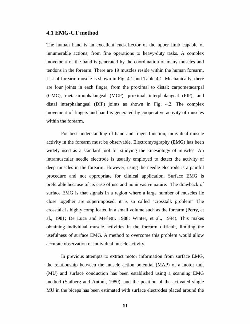
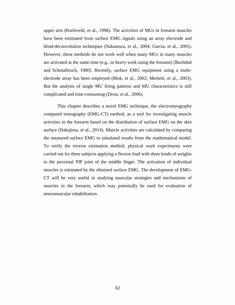
4.1 EMG-CT method .............................................................................................. 61
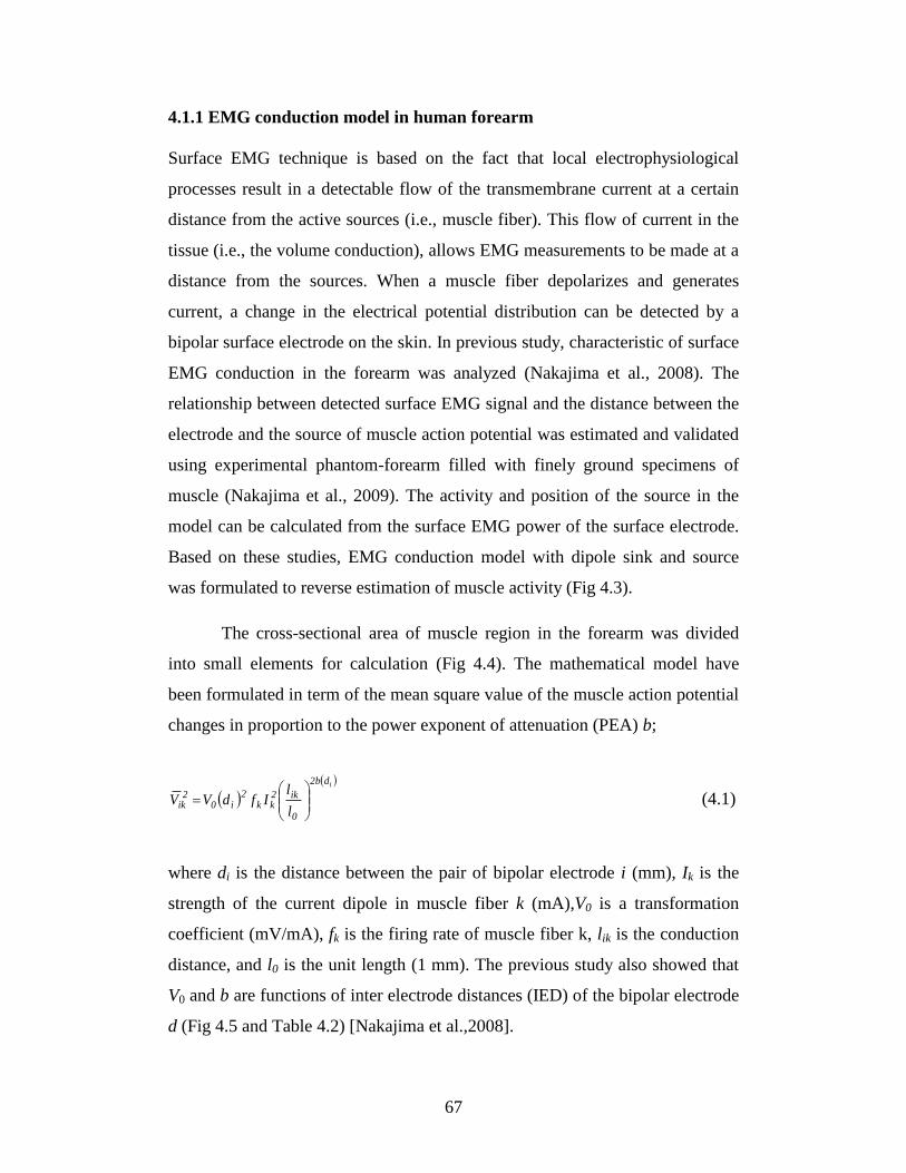
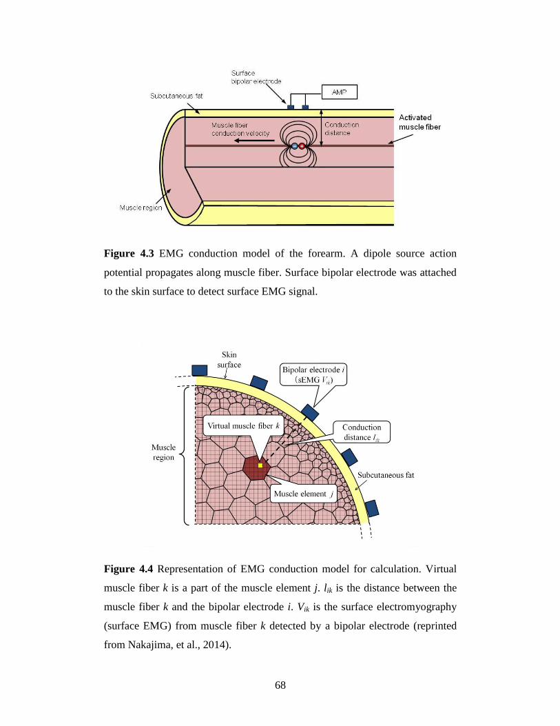
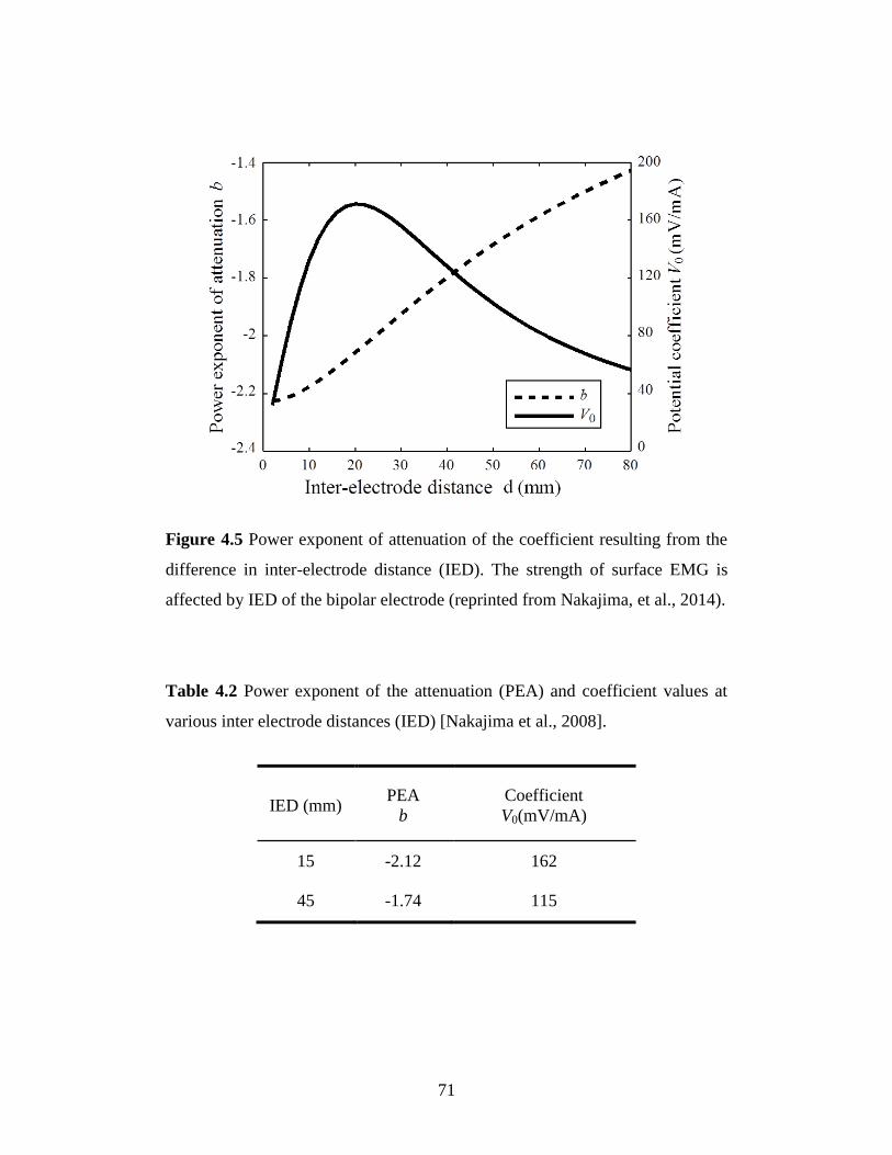
4.1.1 EMG conduction model in human forearm ............................................... 67
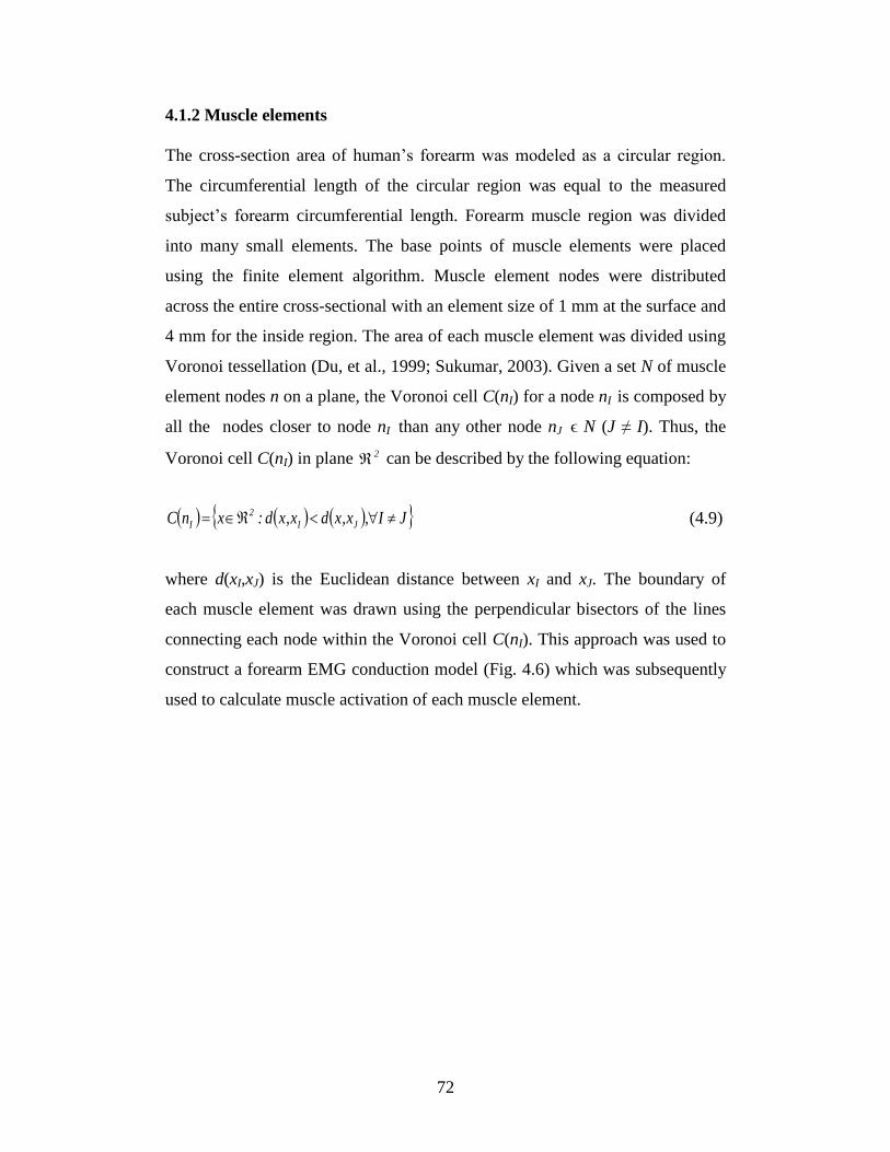
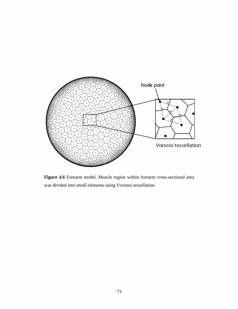
4.1.2 Muscle elements ........................................................................................ 72
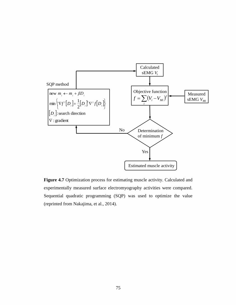
4.1.3 Calculation process .................................................................................... 74
Page 5
ii
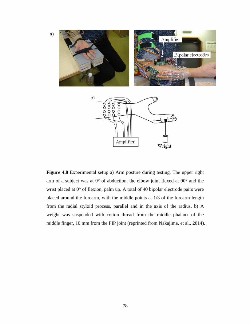
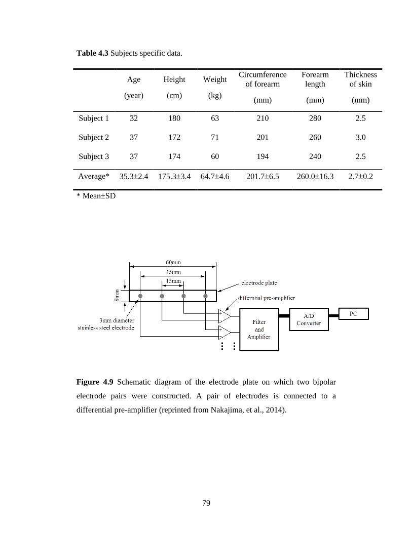
4.1.4 Experimental procedure ............................................................................. 76
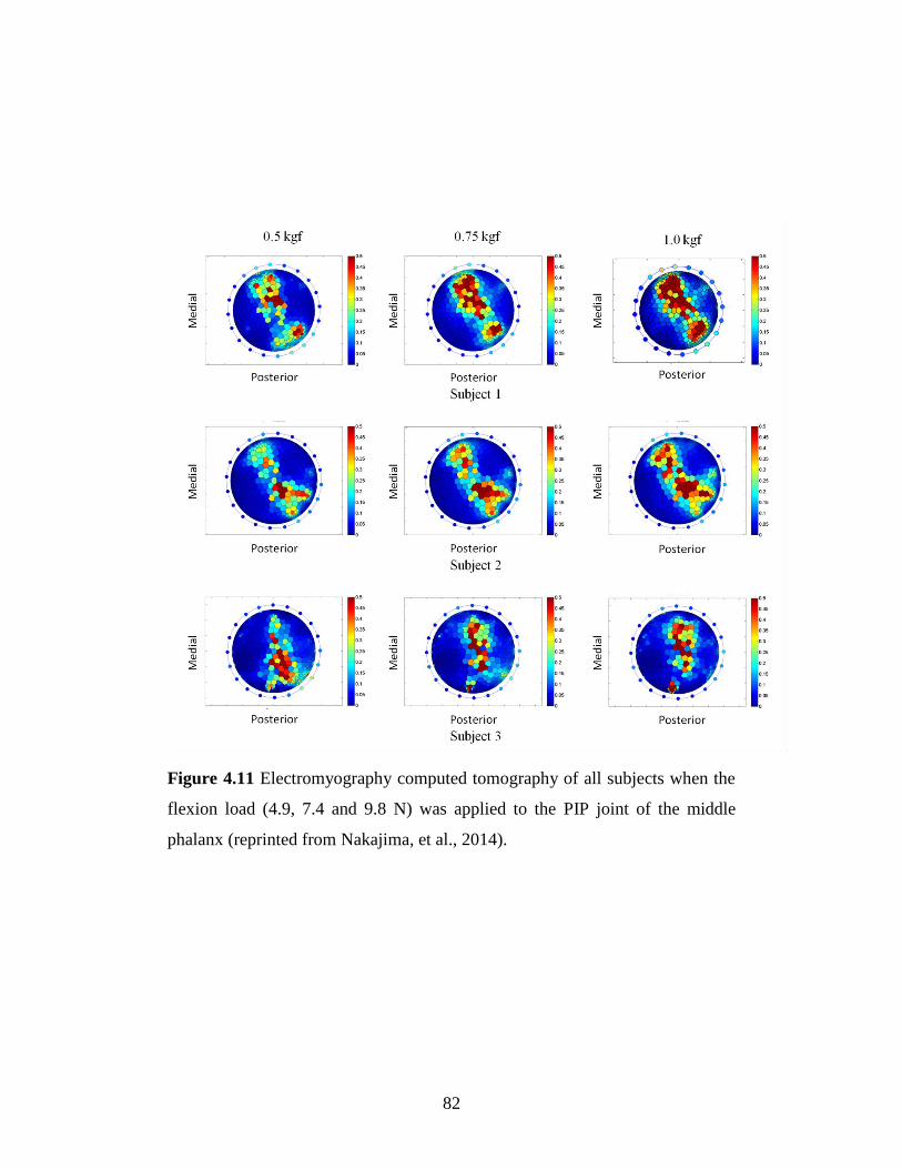
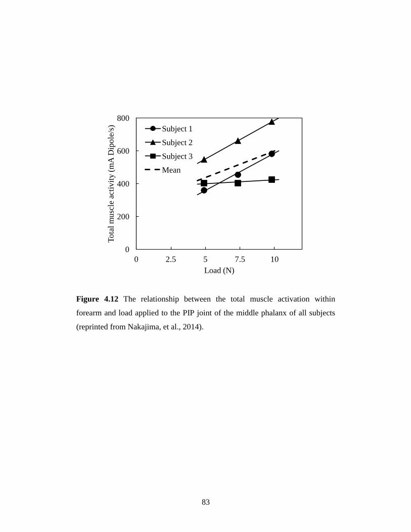
4.2 Results .............................................................................................................. 81
4.3 Discussion ........................................................................................................ 84
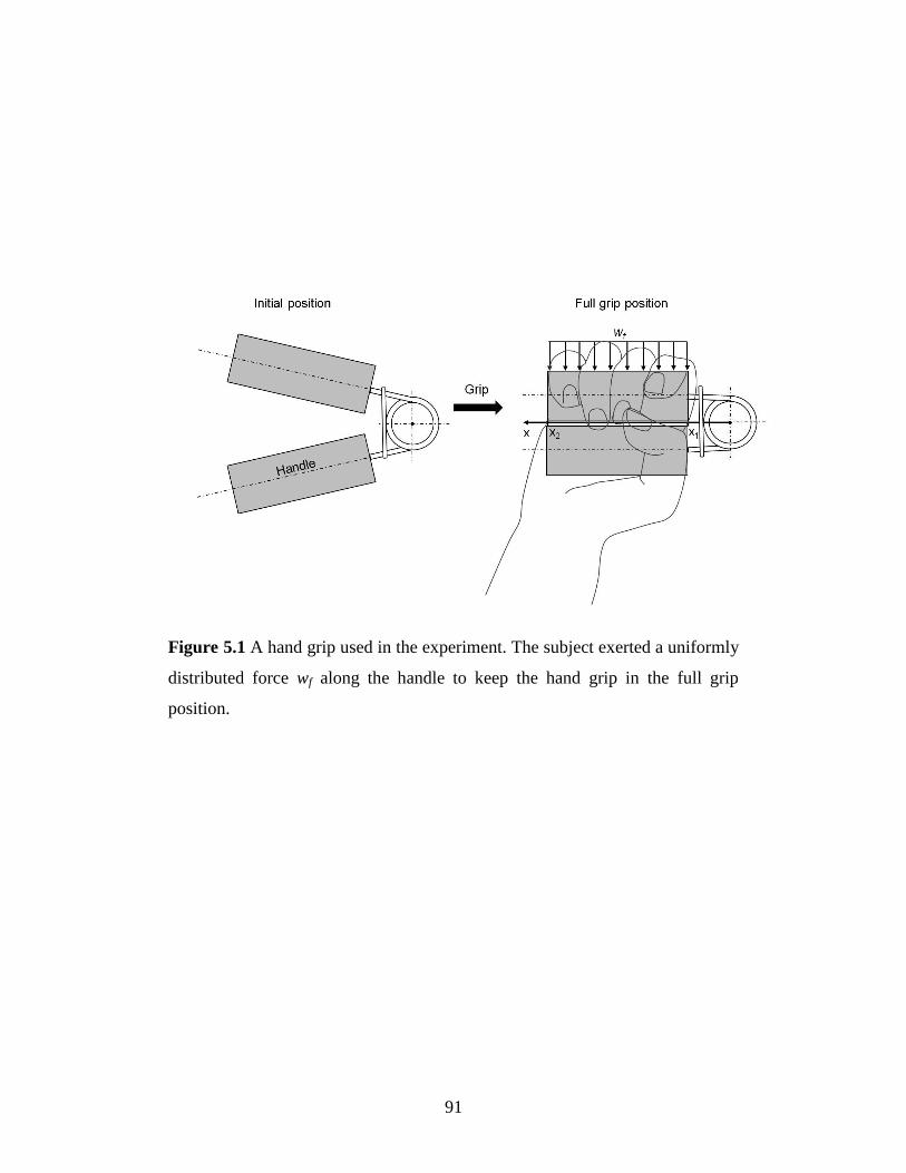
Chapter 5 Muscle Stress Distribution in the Forearm Using
EMG-CT Method .................................................................................. 88
5.1 Stress estimation method .................................................................................. 89
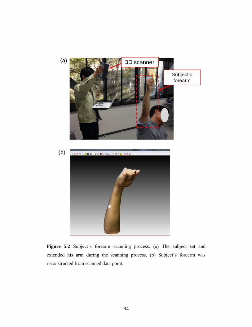
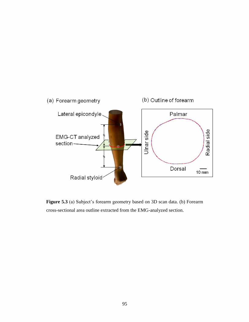
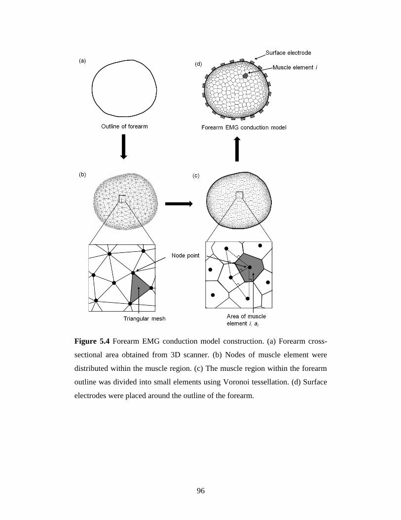
5.1.1 Real shape forearm model construction ..................................................... 92
5.1.2 Muscle activity calculation ........................................................................ 97
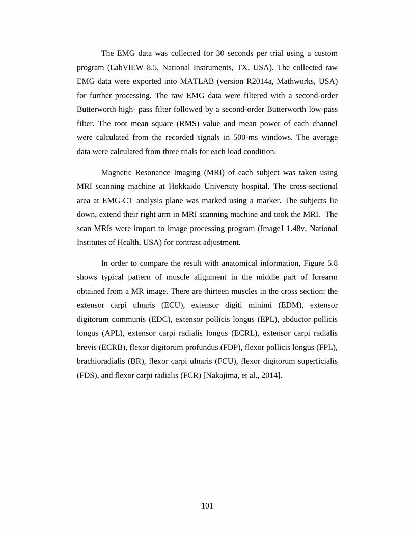
5.1.3 Stress calculation ....................................................................................... 98
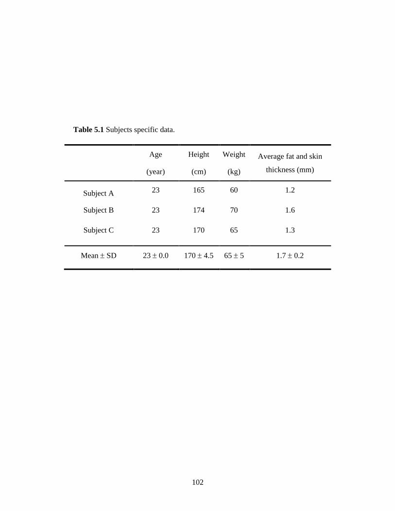
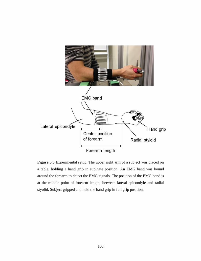
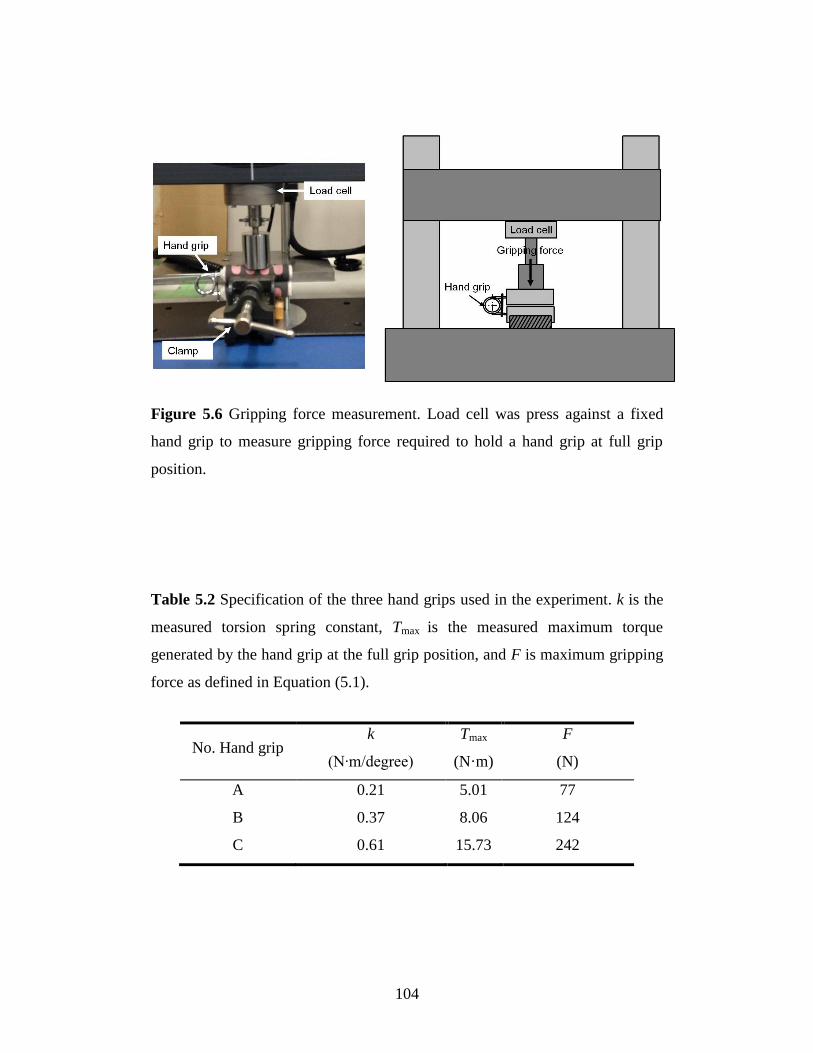
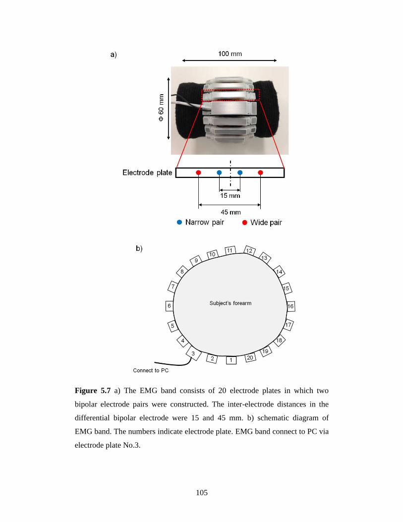
5.2 Experimental procedure ................................................................................. 100
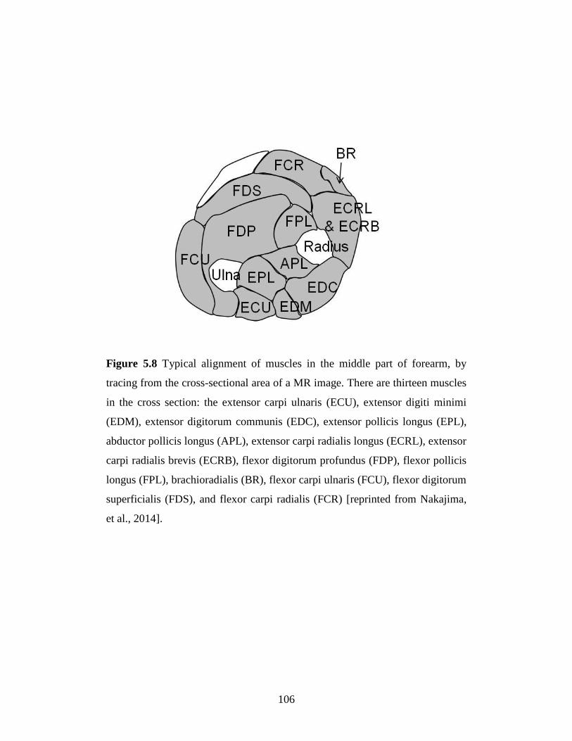
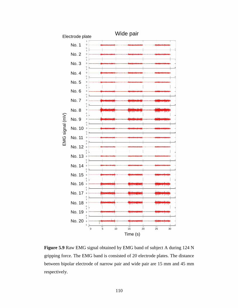
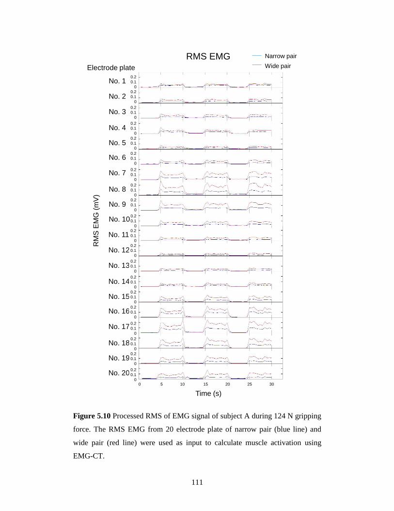
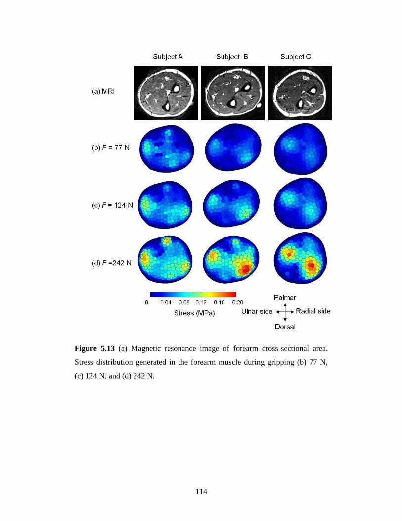
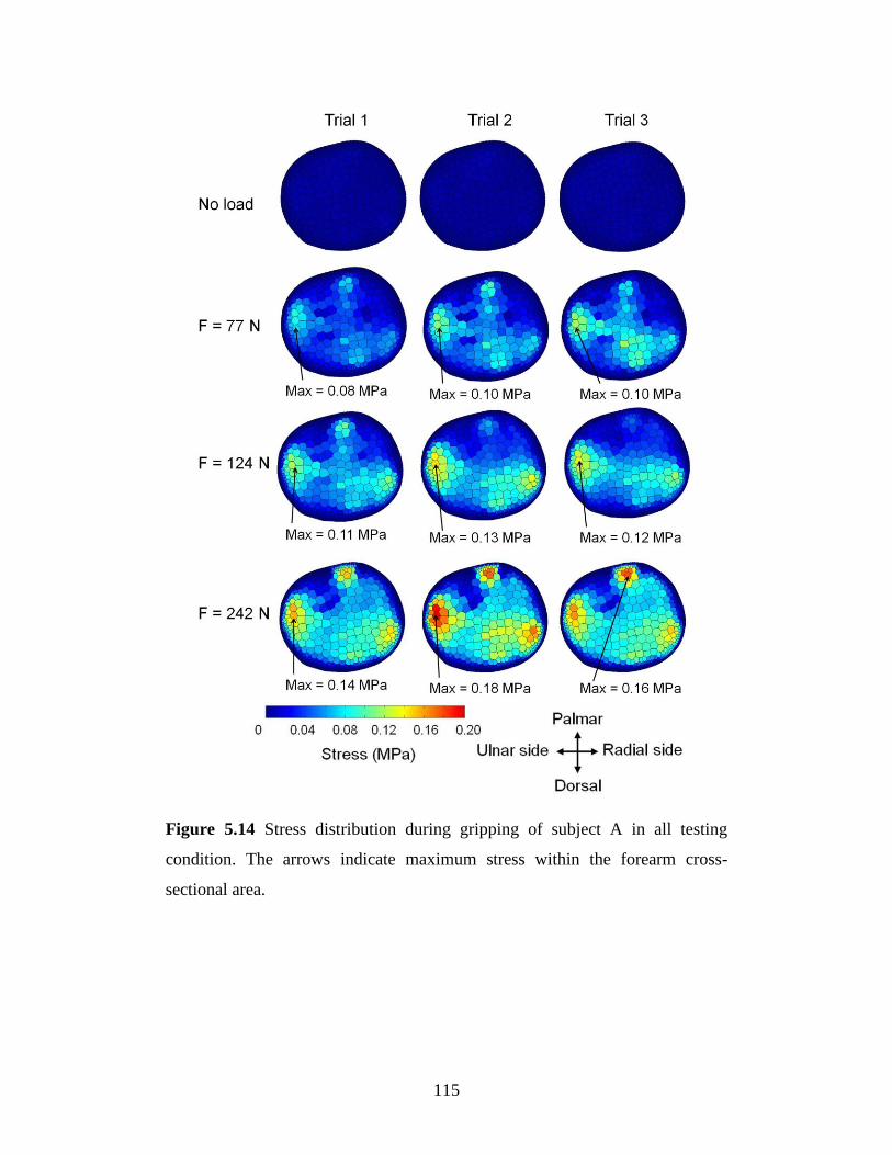
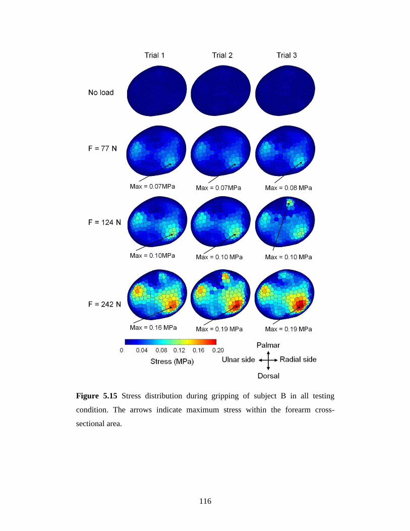
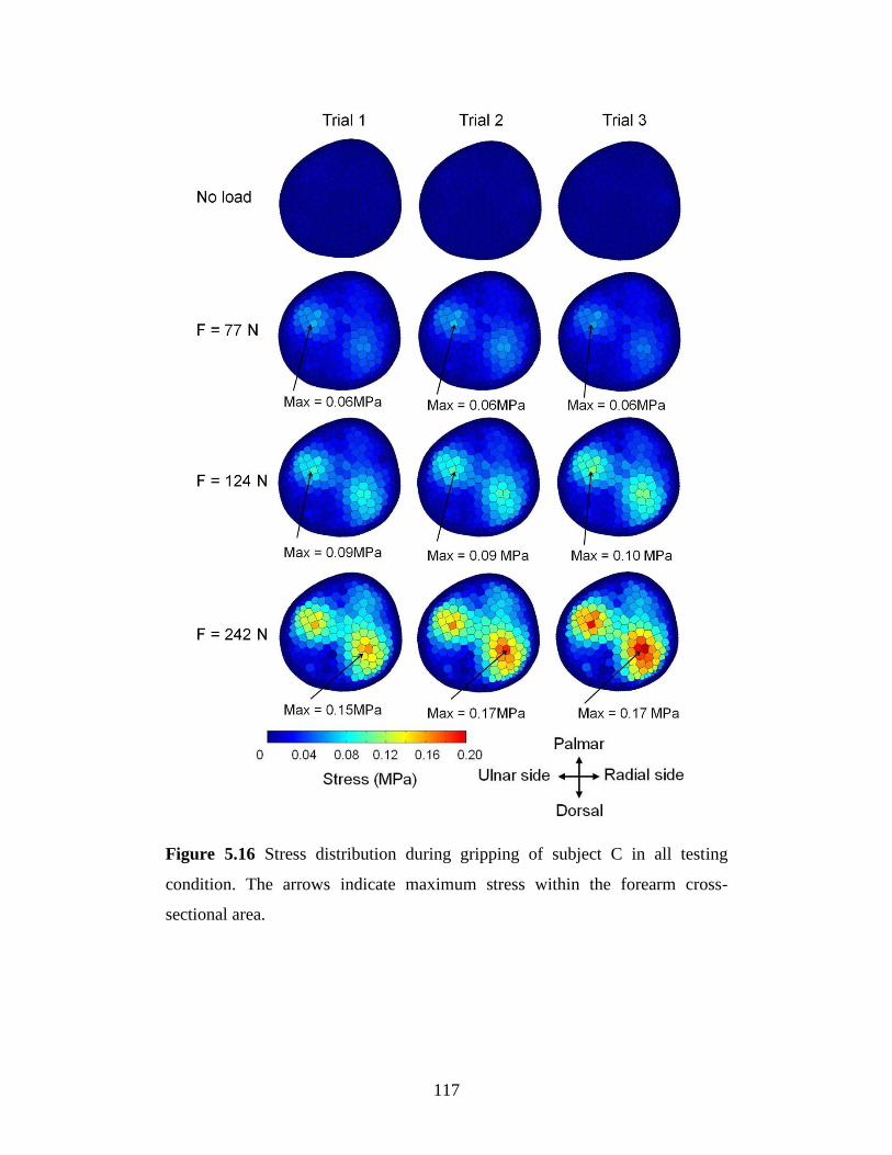
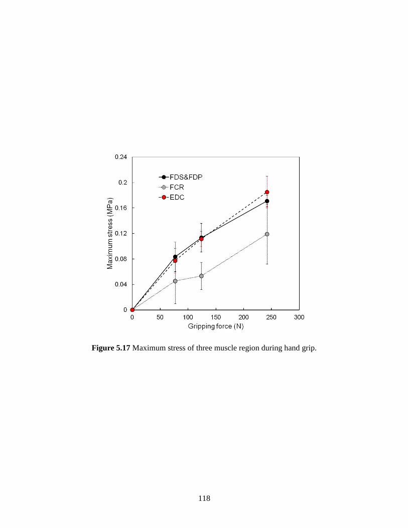
5.3 Results ............................................................................................................ 107
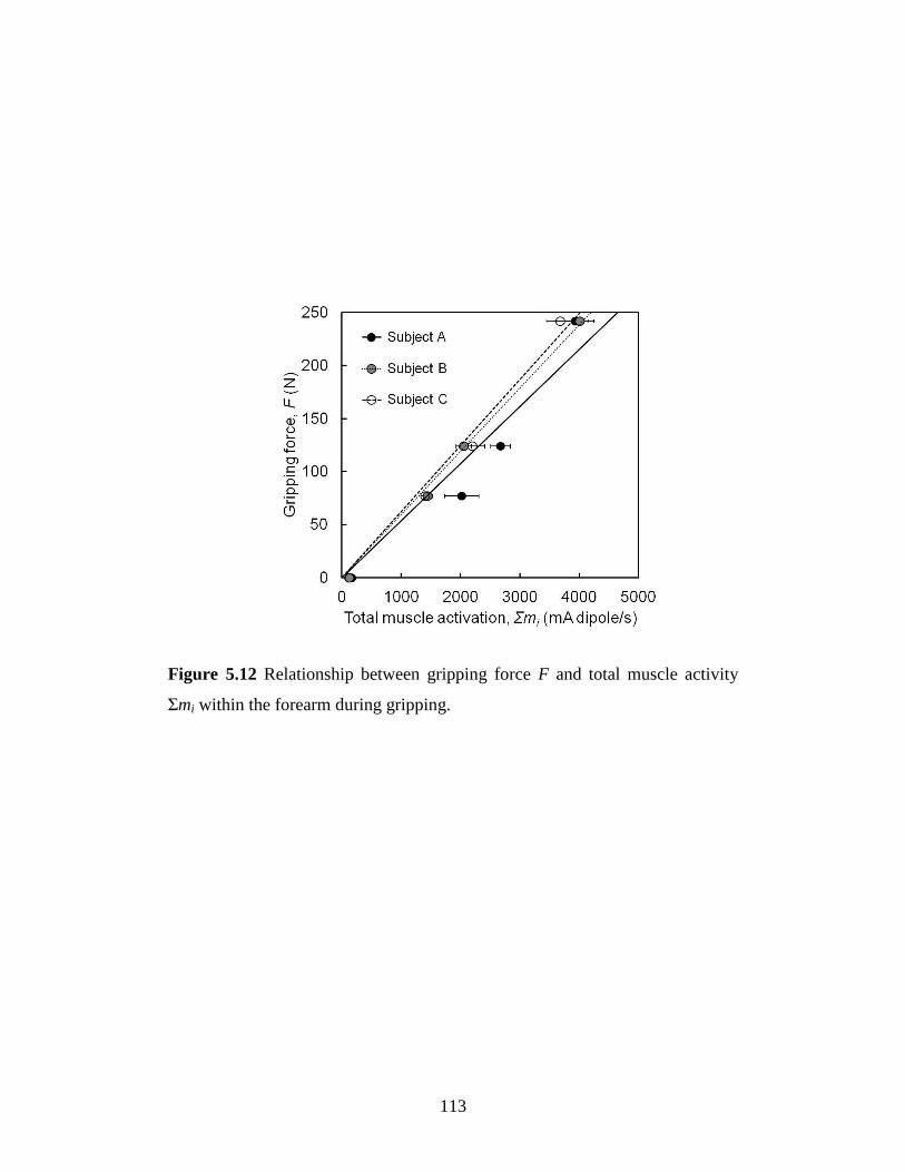
5.3.1 Relationship between muscle force and muscle activity ......................... 119
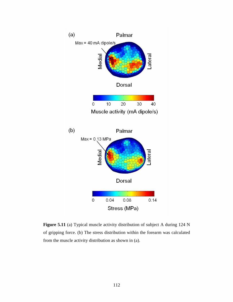
5.3.2 Muscle stress within the forearm ............................................................. 121
5.4 Discussion ...................................................................................................... 125
Chapter 6 Conclusions ........................................................................ 129
6.1 Summary ........................................................................................................ 130
6.2 Future work .................................................................................................... 132
Reference .............................................................................................. 134
Page 6
1
Chapter 1 Introduction
Page 7
2
1.1 Background
Biomechanics is the science that deals with structure and function of living
organism by combining mechanical engineering principles and biological
knowledge. The role of biomechanical engineering is to implement the
knowledge of biomechanics to help in improving the people’s quality of life.
The applications of biomechanics are including clinical application in treatment
or prevention of injury, rehabilitation, ergonomic design and sport.
Muscle is vital to human life. The human strength is determined by the
ability of muscle to exert force. There are more than 500 muscles in a human
body which account for about 43% of the typical body mass. Each muscle has
its own particular role in human movement. The primary purpose of muscle is
to produce force. Skeletal muscles attached to bones by tendon and have the
property of actively contracting and shortening. Human locomotion and muscle
force is strongly correlated. The movement of human body is achieved by
complex cooperation of muscles that cross the joint. The mechanics of muscle
is concerned with the force created in a contraction and the factors that affect
the level of force. The knowledge of “why” and “how” the muscle work is
essential for improved human performance, preventing or treating injury, and
development of effective rehabilitation procedure.
Study of human muscle is the main interest of scientist and
biomechanical engineer for a long time. Muscle mechanics have been studied in
vivo (within a living body), in situ (in the original biological location but with
partial isolation) and in vitro (isolated from a living body). The early work of
studying musculoskeletal system was made by Leonardo da Vinci, who spent
much of his time in the analysis of muscles and their functions. Anatomical
analysis provides the foundation knowledge of muscle. The bodies were
dissected and studies as separate entities. Andreas Vesalius published his
masterpiece work, the Fabrica, providing visual detail of human muscle. In the
past, only basic anatomy was studied but their functional importance was
overlooked. Until recently, the information of muscle could only be obtained
Page 8
3
from cadavers or dead muscle rather than their active state due to the technical
limitation and ethical restrains, not all measurements can be performed on
living human muscle. Studying muscle in vivo requires tool that can observed
muscle while it is still alive.
In the past decades, many researchers are interested in measuring
muscle force during contraction. Direct measurement of muscle force in vivo is
generally impractical and limited to invasive measurement (Ravary, et al.,
2004) such as putting force transducers directly into tendons or ligaments
(Fukashiro, et al., 1993; Finni, et al., 1998; Dennerlein, 2005). These techniques
require surgery which is invasive and impractical. Thus, indirect method base
on predictive model was get more attention from researchers. One of the most
significant muscle research works belongs to A.V. Hill. With 50 years of details
works on muscle mechanics resulting in a Nobel prize in physiology in 1922.
The famous Hill’s model describes the relationship between force-length-
velocity relationships in muscle. His works provide groundwork for human
muscle model which used widely in muscle research.
From a biomechanical standpoint, there is a relation between the
internal muscle force that produces joint moments and the external force that is
human body imparts on a work object. In order to determine the muscle force in
a noninvasive manner, many method based on mathematical models were
developed (Erdemir, et al., 2007). Inverse dynamic model based on linked body
segment has been developed to estimate muscle force (Seireg and Arvikar,
1975; Amis, et al., 1980). With the help of advance computational technology,
the calculation process can be done faster and these models can be used to
estimate joint torque which is the result of all muscle forces acting on that joint.
However, the limitation of inverse dynamic model is that the human joint is a
redundant system with more unknowns than the equilibrium equations. Thus,
the result is usually be total joint torque or total muscle force. To solve this
problem the optimization method has been used to estimate muscle force
(Raikova, 1992; Amarantini and Martin, 2004; Heintz and Gutierrez-Farewik,
Page 9
4
2007). Inverse dynamic model and optimization have proved to be a potential
tool for muscle force estimation. However, without muscle activity involve in
the model it is impossible to specify which muscle generates force during
movement.
The electromyography (EMG) signal was well known to be related to
muscle force generation. The first observation of the relationship between
electricity and muscle contraction was made by Luigi Galvani in 1791. His
experiment showed that frog muscle contraction can be induced by electrical
stimulation. This discovery was the starting point of neurophysiology. The first
to report the detection of surface electrode with a primitive type of
galvanometer was Raymond in 1849. In the last two decades, the method for
detecting and processing EMG signal have been largely refined with the
availability of better equipment, tool and computational techniques and
becoming an important tool for research and clinical applications. Knowledge
of the role of individual muscles in movement is founded on such analysis of
the EMG signal. Using EMG as an indicator of the mechanical function of
muscle is challenged due to the fact that the EMG reflects the electrical, not the
mechanical event of a contraction. However, the application of current
equipment for detecting and processing the signal remains the motivation for
the use of EMG as a tool for measuring of muscle force.
Overused of muscle or disease can cause muscle dysfunction, limiting
the ability of movement. Identifying the impaired muscle during contraction is
important for effective treatment. However, sense of human is limited; sensor
or scientific tool is required to improve the ability to observe muscle activity.
One of the roles of biomechanical engineer is to provide tools for studying
muscle function. Currently there is no practical tool ready for muscle force
measurement. Development of method to estimate muscle force will be very
useful in both biomechanical and medical fields.
Page 10
5
1.2 Scope and aim of this study
To understand how muscles work together, it is required a tool that can “see”
the activity of muscle and a method to “measure” individual muscle force.
Using surface EMG signal which detected from skin surface is one way to
measure muscle activity in a non-invasive manner. In recent years method for
detecting and processing EMG signal have been improved considerably. The
aim of this research is to develop methods to estimate muscle forces using
surface EMG signal. In this thesis, a series of study and research were
conducted to achieve the aim.
The main focus of this study is muscle force during human locomotion
in daily activity such as carrying an object, using a hand tool and walking.
Upper and lower limb are the important parts of the human body that defines
the dexterity. The development of a method to estimate muscle force from
EMG required knowledge of many aspects, starting from EMG detection
technique, interpretation of the detected signals, and understanding the
relationship between muscle force and EMG signal. A practicable muscle force
estimation technique called EMG-driven model was developed and
implemented to estimate muscle force during elbow and knee joint movement.
EMG signal from the muscles were measured by pairs of bipolar electrode and
used to estimate muscle force. The results show the effect of dynamic motion
on the EMG signals. Increasing in muscle force or movement speed affects the
amplitude of EMG signal. It seems that EMG-driven model is practical in
estimate muscle force in major joint where surface EMG signals from muscles
are detectable, like those of the upper arm and legs. However, in the human
forearm, there are many muscles that are used to control the complex
movement of fingers and hand. These muscles are relatively small and difficult
to detect by conventional surface electrode. The problem of detecting unwanted
signals or cross-talk is the main problem in assessing muscle activity in forearm
region.
Page 11
6
To overcome the cross-talk problem a novel method called
electromyography computed tomography (EMG-CT) was developed to measure
individual muscle activity within the deep forearm region using multi surface
electrode (Nakajima, et al., 2014). This developed method provides a tool to
visualize muscle activity within the forearm. The present study developed a
method to estimate muscle stress i.e., force generated during contraction per
unit area in the whole cross-section of the forearm during hand action using
EMG-CT, the relationship between force and muscle activity during gripping
was investigated. A model related muscle activity and force was developed.
Muscle stress, was estimated during hand gripping. This method provides a new
way of measuring muscle stress in the human forearm.
Page 12
7
Chapter 2 Muscle Physiology and
Electromyographic Phenomena
Page 13
8
2.1 Muscle physiology
An understanding of musculoskeletal systems and their mechanical properties is
important in biomechanics study. Anatomy study provides essential information
for musculoskeletal structures and joint motions relate to human movement.
Skeletal muscle varies in shape, size, and function. The role of skeletal muscle
is to act as motor that move the bones about joint. Muscles are attached to
bones by tendons. When muscle contracts, force transmit from one bone to
another through joint and generate motion. The human body can be represented
as a system of articulated segments in static or dynamic balance. Mechanically,
there are three main types of muscle contractions: isometric, isotonic, and
isokinetic. During isometric contraction, muscle develops tension without
shortening. Isotonic refers to muscle developing a constant tension, and
isokinetic is a muscle contraction at a constant velocity. A concentric action
occurs when the torque that muscle group makes is larger than the torque of a
resistance, resulting in muscle shortening. An eccentric muscle action is the
lengthening of an activated muscle.
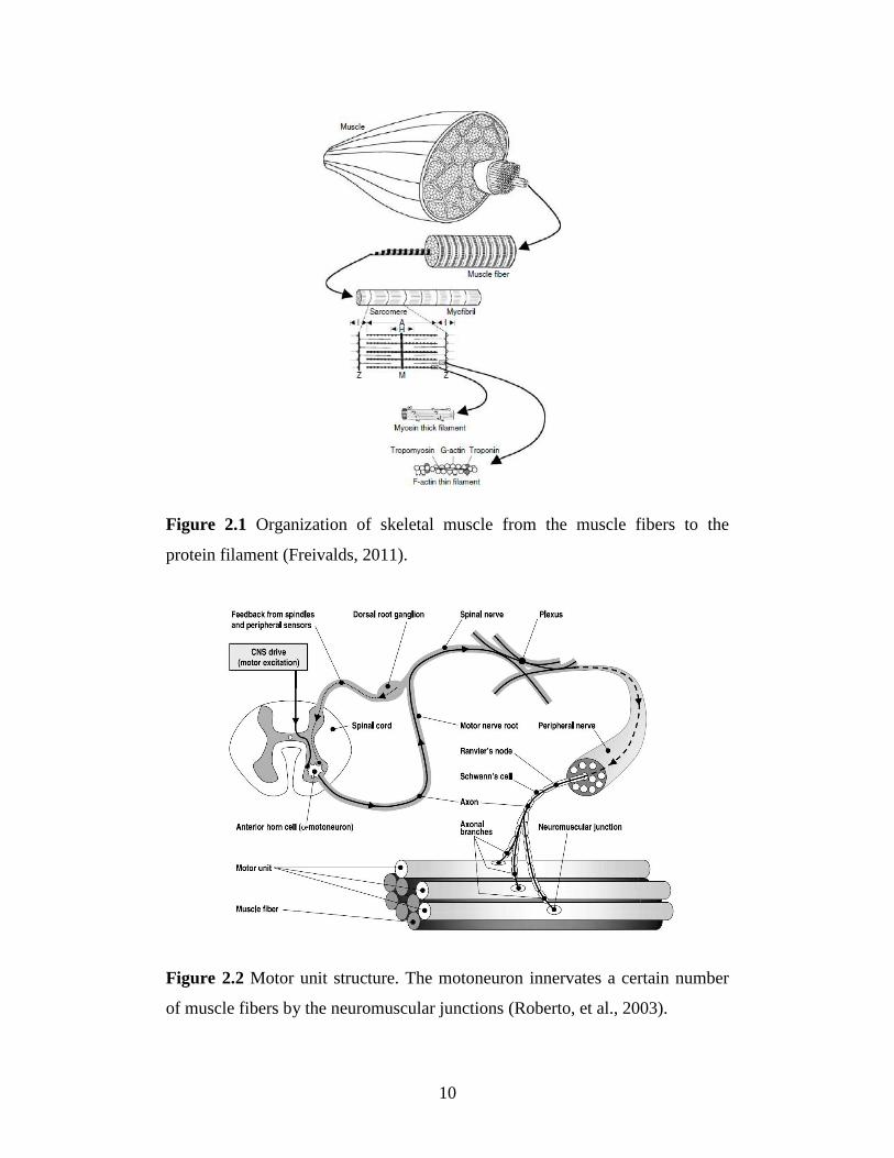
Skeletal muscle is hierarchically organized, as shown in Fig. 2.1.
Muscle is composed of a large number of muscle fibers. Each fiber also
contains many myofibrils. The myofibril contains a series of sarcomeres that
make the striated appearance of skeletal muscle. The active tension of whole
muscles based on the interaction of two contractile proteins in sarcomeres i.e.
actin and myosin. Cross-bridges between myosin and actin are attached and
detached with chemical energy stored in adenosine triphosphate (Huxley and
Hanson, 1954). This mechanism generates tension within a muscle fiber.
The tension created by a muscle contraction also depends on the length
of the muscle, and the velocity of contraction. A muscle produces the maximum
amount of tension when it is lengthened slightly beyond resting length. In
concentric muscle contractions, a muscle can produce less tension as shortening
velocity increases. In eccentric muscle contraction, the maximum tension a
muscle can produce increases as the speed of lengthening increases.
Page 14
9
Motor unit (MU) is the basic building block for the production of force
and movement, both in reflex and voluntary contractions. MU is defined as a
set of muscle fibers innervated by the same motoneuron as shown in Fig 2.2.
MU can vary in size considerably. The MUs are distributed throughout the
cross-sectional area of the muscle. The amount of force and power generated by
muscle is directly related to the type, number, and size of motor units in the
muscle. There are two type of muscle fiber in mammalian skeletal: slow twitch
motor unit (Type I) which are recruited for light to moderate intensity activity
and fast twitch motor unit (Type II) which capable of high force production and
fast contraction speed.
The force and velocity of body movement is controlled by motor unit
recruitment and rate coding. Slow twitch motor units are recruited first and the
fast twitch fatigable units are recruited only when fast powerful movement is
required. Each time a contraction is repeated, a particular motor unit is recruited
at the same force level. At high force levels after every motor units have been
recruited, additional force is generated by increasing the firing frequencies of
the motor units.
Page 15
10
Figure 2.1 Organization of skeletal muscle from the muscle fibers to the
protein filament (Freivalds, 2011).
Figure 2.2 Motor unit structure. The motoneuron innervates a certain number
of muscle fibers by the neuromuscular junctions (Roberto, et al., 2003).
Page 16
11
2.2 Electromyographic phenomena
Electromyography (EMG) is the study of muscle function through the electrical
signal that the muscles emanate. EMG has been used in studying of muscle
function and in clinical application such important topics as musculoskeletal
injury, carpal tunnel syndrome, and muscle fatigue. Modern instrumentation
has been developed to facilitate easy acquisition of EMG data. Surface
electrode is usually used to measure EMG signal from skin surface due to its
non-invasive and ease of use. In the past decades, EMG study progress
significantly. However, the interpretation of EMG signals stills has many issues
unresolved.
2.2.1 Origin of EMG signal
Muscle fibers are active by the central nervous system through electric signals
transmitted by motoneurons. A chain of events occur before a muscle fiber
contracts. Each muscle fiber is surrounded by a plasma membrane called the
sarcolemma. The excitability of muscle fibers through neural control can be
explained by a model of a semi-permeable membrane describing the electrical
properties of the electrical properties of sarcolemma. Central nervous system
activity initiates a depolarization in the motoneuron. The depolarization is
conducted along the motoneuron to the muscle fiber’s motor endplate. At the
endplate, a chemical substance is released causing a rapid depolarization of the
muscle fiber under the motor endplate. Resulting in depolarization of the
muscle fiber membrane which triggers muscle contraction (Lucas, 1909). This
rapid depolarization, and the subsequent repolarization of the muscle fiber, is an
action potential. The propagated action potential spreads along the sarcolemma
and into the muscle fiber. The EMG signal is based on action potentials at the
muscle fiber membrane resulting from depolarization/repolarization processes.
In order to study EMG signal generated from muscle fiber. EMG
technique is based on the fact that local electrophysiological processes result in
a detectable flow of the transmembrane current at a certain distance from the
Page 17
12
active sources (i.e., muscle fiber). This flow of current in the tissue (i.e., the
volume conduction), allows EMG measurements to be made at a distance from
the sources. The principle of volume conductivity is important. In general, the
simplest model used to interpret extracullular action potentials of muscle is the
dipole concept (R, 1947; Plonsey, 1974). The basis of surface EMG is the
relationship between the action potentials of muscle fibers and the extracellular
recording of those action potentials at the skin surface. Electrodes external to
the muscle fiber can be used to detect action potentials.
Page 18
13
2.2.2 Surface EMG detection technique
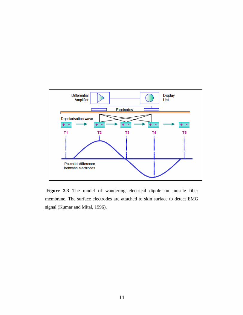
When muscle generates force, there are electric signals that generated and
propagate along muscle fiber; these signals can be detected by placing electrode
on the skin surface (Fig. 2.3). Surface electrodes are generally used in the
bipolar configuration. In bipolar electrode configuration, two electrodes are
used at the detection site and a third common-mode reference, or ground
electrode is placed distally in a neutral electrical environment. This
arrangement of electrodes is dictated by the use of a differential preamplifier as
the means of signal amplification. The differential preamplifier increased the
amplitude of the difference signal between each of the detecting electrodes and
the common mode reference. Signals that are common to both detection
electrode sites are termed common mode signals and produce a nearly zero
preamplifier output. This desirable characteristic of differential preamplifiers
significantly improves the signal-to-noise ratio of the measurement and allows
the detection of low level EMG potentials in noisy environment.
The observed EMG signal is filtered by the tissue and the electrode in
the process of being detected, it is necessary to amplify it. This might affect the
frequency characteristics of the signal. It is important to note that the
characteristics of the observed EMG signal are a function of the apparatus used
to acquire the signal as well as the electrical current which is generated by the
muscle fibers.
Page 19
14
Figure 2.3 The model of wandering electrical dipole on muscle fiber
membrane. The surface electrodes are attached to skin surface to detect EMG
signal (Kumar and Mital, 1996).
Page 20
15
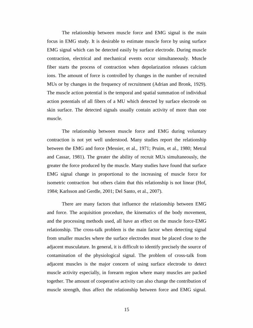
The relationship between muscle force and EMG signal is the main
focus in EMG study. It is desirable to estimate muscle force by using surface
EMG signal which can be detected easily by surface electrode. During muscle
contraction, electrical and mechanical events occur simultaneously. Muscle
fiber starts the process of contraction when depolarization releases calcium
ions. The amount of force is controlled by changes in the number of recruited
MUs or by changes in the frequency of recruitment (Adrian and Bronk, 1929).
The muscle action potential is the temporal and spatial summation of individual
action potentials of all fibers of a MU which detected by surface electrode on
skin surface. The detected signals usually contain activity of more than one
muscle.
The relationship between muscle force and EMG during voluntary
contraction is not yet well understood. Many studies report the relationship
between the EMG and force (Messier, et al., 1971; Pruim, et al., 1980; Metral
and Cassar, 1981). The greater the ability of recruit MUs simultaneously, the
greater the force produced by the muscle. Many studies have found that surface
EMG signal change in proportional to the increasing of muscle force for
isometric contraction but others claim that this relationship is not linear (Hof,
1984; Karlsson and Gerdle, 2001; Del Santo, et al., 2007).
There are many factors that influence the relationship between EMG
and force. The acquisition procedure, the kinematics of the body movement,
and the processing methods used, all have an effect on the muscle force-EMG
relationship. The cross-talk problem is the main factor when detecting signal
from smaller muscles where the surface electrodes must be placed close to the
adjacent musculature. In general, it is difficult to identify precisely the source of
contamination of the physiological signal. The problem of cross-talk from
adjacent muscles is the major concern of using surface electrode to detect
muscle activity especially, in forearm region where many muscles are packed
together. The amount of cooperative activity can also change the contribution of
muscle strength, thus affect the relationship between force and EMG signal.
Page 21
16
The activation patterns of individual muscles are not representative of all
muscles in the same functional group, and there are differences in how muscles
within a muscle group respond to training. Even individual muscle is quite
sophisticated, with different motor unit activation depending on the task or
muscle action. Type of contraction either isometric or anisometric and either
isotonic or anisotonic also affect the relationship between EMG and muscle
force. The used of EMG as a tool for determining the force is challenging due
to complexity and variability in biological signals.
Page 22
17
Chapter 3 An EMG-Driven Model for
Estimating Muscle Force
Page 23
18
3.1 EMG-driven model
In order to determine the muscle forces in a noninvasive manner, many
methods based on mathematical models were developed (Erdemir, et al., 2007).
The electromyography (EMG) signal was well known to be related to muscle
force generation. EMG-to-force processing was well described by Hof and Van
Den Berg (1981) and thus, EMG was introduced into the model to estimate the
muscle force. The advantage of the EMG-driven model is that the processed
EMG signal reflects the activation of each muscle crossing the joint, thus
facilitating the accurate estimation of the individual muscle force. Interest in the
EMG-driven model has grown recently after it was proven to be a powerful tool
to estimate the muscle force in various movements (White and Winter, 1992;
Feng, et al., 1999; Lloyd and Besier, 2003; Shao, et al., 2009).
An important part of the EMG-driven model is the musculotendon
model, which indicates that, the change in length of muscle during contraction
affects the potential force that a muscle can generate. The popular Hill-type
muscle model is usually used to describe the contraction mechanism of the
muscle. Muscle model parameters such as maximum isometric force (F0),
optimum muscle length (LFOPT), and maximum shortening velocity (v0)
represent muscle force-length-velocity relationships. The accuracy of the
estimated muscle force in the EMG-driven model depends on how well we
estimate these parameters. However, muscle model parameters vary among
individuals. Thus, a tuning process is required to estimate the appropriate value.
Some researchers obtained these parameters by using calibration trials and
optimization processes to tune the parameters (White and Winter, 1992; Lloyd
and Besier, 2003; Shao, et al., 2009). The tuning process provides a set of
muscle model parameters that account for a limit movement conditions. It has
never been examined whether they can be applied to estimate the muscle force
with respect to a different speed than that used in the calibration trials. As the
knowledge of the manner in which muscle parameters respond to the change of
Page 24
19
movement velocity is still limited, using the same set of parameters for different
conditions can be problematic.
The influence of changing movement velocity on the muscular activity
has been investigated. During repetitive movement such as cycling and
walking, muscles in lower-limb increased their EMG activity level as the
movement rate increased (Neptune, et al., 1997; Hof, et al., 2002). High-speed
muscle contractions have been showed to enhanced EMG activities in the
shoulder and leg muscles (Carpentier, et al., 1996; Laursen, et al., 1998;
Brindle, et al., 2006). These finding demonstrate that there is a velocity effect
on muscle force generation. Therefore, it is expected that changing the
movement velocity or rate-effect would have an effect on muscle model
parameters. Change in velocities has very important implication in sports,
rehabilitation, ergonomics and treatment of motor unit disorders. In addition,
the ability to change the velocity of ongoing movement is important feature to
perform a proper daily activity. Thus, to confidently use the EMG-driven
model, validation of the rate-effect on the muscle model parameters is required.
In the present study, we aimed to develop an EMG-driven model to
estimate the muscle force during elbow and knee flexion/extension movement,
and to determine the influence of the rate-effect on the model parameters of the
Hill-type muscle model. The muscle model parameters were estimated using an
EMG-driven model technique in combination with experimental measurements
and an optimization process. The optimization process was used to minimize
the difference between the estimated and the experimental results, by fitting the
value of muscle parameters at various movement frequencies. We believe that
the information derived from this study will be useful in modeling the dynamic
performance of muscles and improving the existing model.
Page 25
20
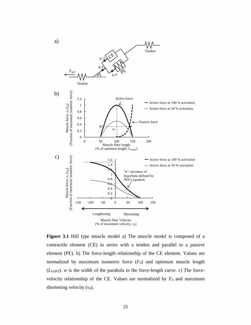
The muscle-tendon unit is composed of muscle fiber in series with the
tendon, following the musculotendon model as described by Zajac (Zajac,
1989). The Hill-type model is composed of a contractile element (CE) in
parallel with a passive element (PE) that is in series with the tendon (Fig. 3.1a).
Thus, the force in the musculotendon unit, FMT can be represented by:
cosFFcosFFF PECEMtMT (3.1)
where Ft is the tendon force; FM is the sum of forces in the CE (FCE) and the PE
(FPE); the pennation angle, is the angle between the lines of action of the
tendon and the muscle fiber. FCE can be estimated by the generalized function:
tvlFF EMGMvMl0CE (3.2)
wherem0 σPCSAF , F0 is the maximum isometric force that the model can
generate, which is a function of the physiological cross-section area (PCSA)
and maximum muscle stress, σm. αl(lM) is the fraction of the F0 that the muscle
can produce at the current length, lM (Figure 3.1b). αv(vM) is the fraction of F0
that the muscle can produce at the current velocity vM (Figure 3.1c). αEMG(t) is
the muscle activation measured from the EMG signal. The normalized force-
length relationship, αl(lM) was calculated as described by Gallucci and Challis
(2002), and is shown below:
2
FOPT
FOPTMMl
Lw
Ll1l
(3.3)
where is the optimum length of muscle fiber and is a parameter
specifying the width of the force-length relationship. For the force-velocity
relationship, Hill proposed a relationship between tension and muscle velocity
Page 26
21
Figure 3.1 Hill type muscle model a) The muscle model is composed of a
contractile element (CE) in series with a tendon and parallel to a passive
element (PE). b) The force-length relationship of the CE element. Values are
normalized by maximum isometric force (F0) and optimum muscle length
(LFOPT). w is the width of the parabola in the force-length curve. c) The force-
velocity relationship of the CE. Values are normalized by F0 and maximum
shortening velocity (v0).
0
0.2
0.4
0.6
0.8
1
1.2
1.4
1.6
-150 -100 -50 0 50 100 150
0
0.2
0.4
0.6
0.8
1
1.2
0 50 100 150 200
Passive force
Muscle fiber length (% of optimum length, LFOPT)
Musc
le f
orc
e, α
l(l
M)
(Fra
ctio
n o
f m
axim
um
iso
met
ric
forc
e)
w
b)
Muscle fiber Velocity (% of maximum velocity, v0)
Musc
le f
orc
e, α
v(v
M)
(Fra
ctio
n o
f m
axim
um
iso
met
ric
forc
e)
ShorteningLengthening
c)
“n” curvature of
hyperbola defined by Hill’s equation
Active force
a)
Tendon
Tendon
FMT
Active force at 100 % activation
Active force at 50 % activation
Active force at 100 % activation
Active force at 50 % activation
Page 27
22
and described it by the equation (Hill, 1938):
baFbvaF 0MM (3.4)
where a and b are Hill’s constants normalized to F0 and maximum shortening
velocity v0 respectively. The shape parameter in Hill’s equation can be
described by the ratio n = a/F0 = b/v0. The value of n ranges between 0.2 and
0.8 (White and Winter, 1992) thus, for concentric condition Hill’s equation was
rewritten in the form:
M0
M0
Mvvvn
vvnv
, concentric (3.5)
for eccentric form of the force-velocity relationship the equation was presented
by FitzHugh (1977) as:
0M
M0
Mvvn2v
vvn0.51.5v
, eccentric (3.6)
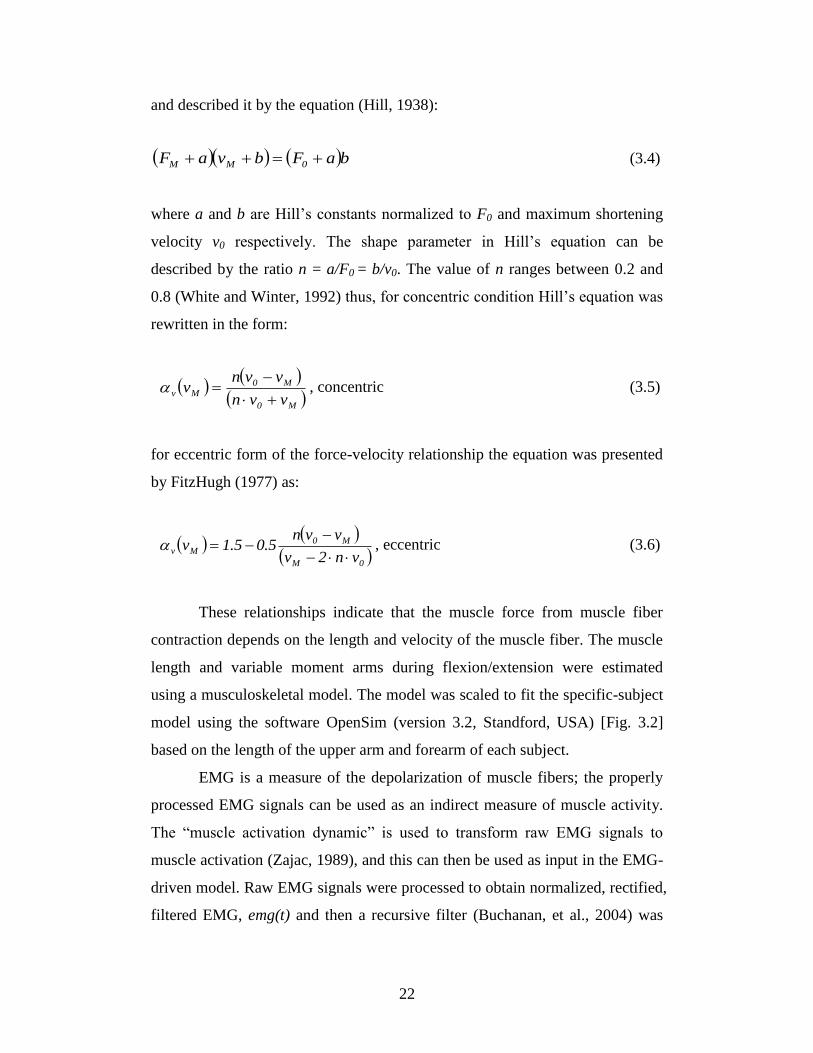
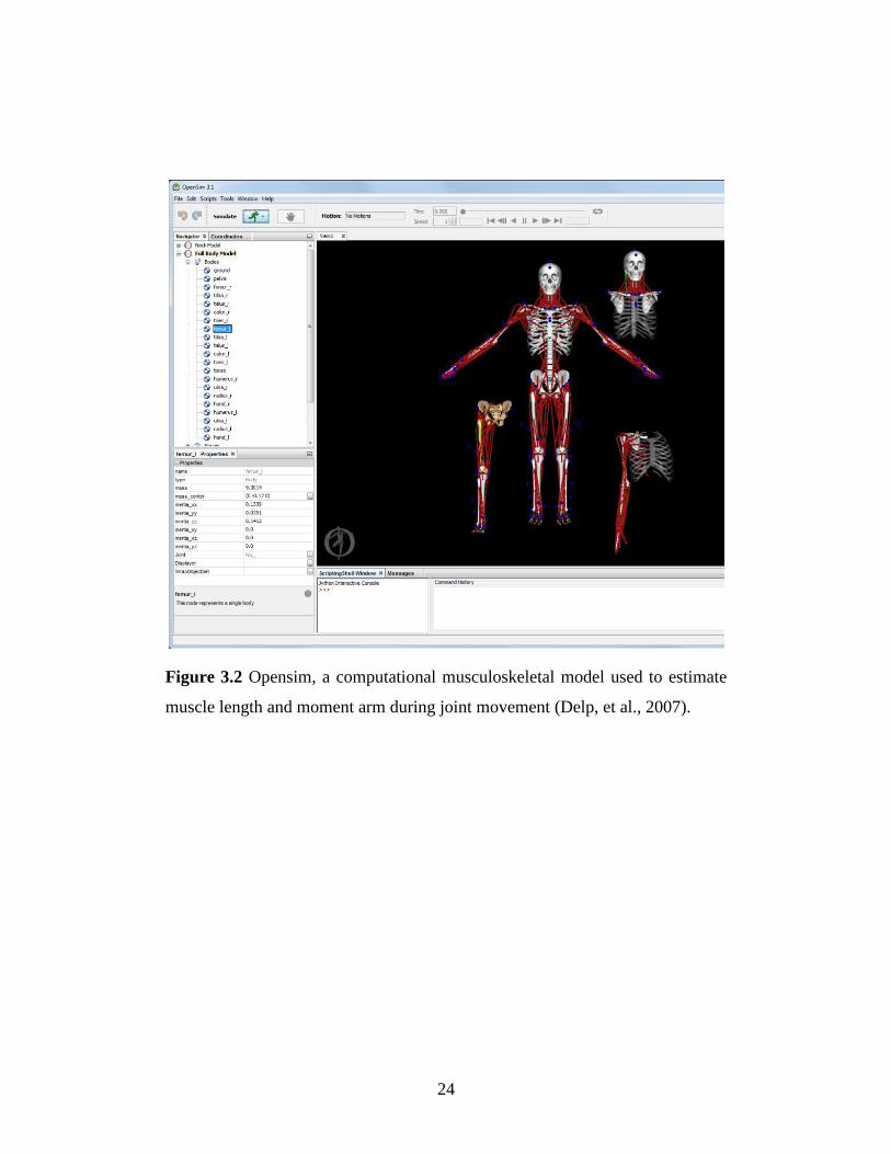
These relationships indicate that the muscle force from muscle fiber
contraction depends on the length and velocity of the muscle fiber. The muscle
length and variable moment arms during flexion/extension were estimated
using a musculoskeletal model. The model was scaled to fit the specific-subject
model using the software OpenSim (version 3.2, Standford, USA) [Fig. 3.2]
based on the length of the upper arm and forearm of each subject.
EMG is a measure of the depolarization of muscle fibers; the properly
processed EMG signals can be used as an indirect measure of muscle activity.
The “muscle activation dynamic” is used to transform raw EMG signals to
muscle activation (Zajac, 1989), and this can then be used as input in the EMG-
driven model. Raw EMG signals were processed to obtain normalized, rectified,
filtered EMG, emg(t) and then a recursive filter (Buchanan, et al., 2004) was
Page 28
23
used to determine the neural activation value, u(t). This process can be
approximated by a discrete eqaution:
2tuβ1tuβdtemgαtu 21t (3.7)
where d is the electromechanical delay, αt, and β1 and β2 are coefficients that
define the second-order dynamics. In the present study, the relationship
between EMG and muscle activation was defined by an exponential
relationship (Lloyd and Besier, 2003), where A is a non-linear shape factor
constrained to -3<A<0, and is described as:
1e
1et
A
tuA
EMG
(3.8)
The passive force from PE (FPE) can be represented by the exponential
relationship described by Schutte (1993):
5
1/Ll10
0mPEe
eFlF
FOPTM
(3.9)
Muscle force from each muscle can be calculated by muscle model
described above.
Page 29
24
Figure 3.2 Opensim, a computational musculoskeletal model used to estimate
muscle length and moment arm during joint movement (Delp, et al., 2007).
Page 30
25
3.2 Muscle force estimation during elbow joint movement
Upper-limb motion is essential for performing daily activities, such as eating,
drinking, washing of the face, brushing of the teeth and pushing/pulling objects.
Any disability of the upper limb will limit the activities that a person can
perform, thus making it difficult of an individual to lead a normal life. The
elbow is an important mechanical link in the upper limb. The flexion/extension
motion of the elbow primarily results from the reaction forces generated by the
biceps and triceps. Knowledge of muscle mechanics is required for designing
effective exercise training programs and developing rehabilitation procedures.
In order to enhance our understanding of the muscle mechanics during elbow
joint movement, the estimation of muscle force of the biceps and triceps in vivo
is necessary.
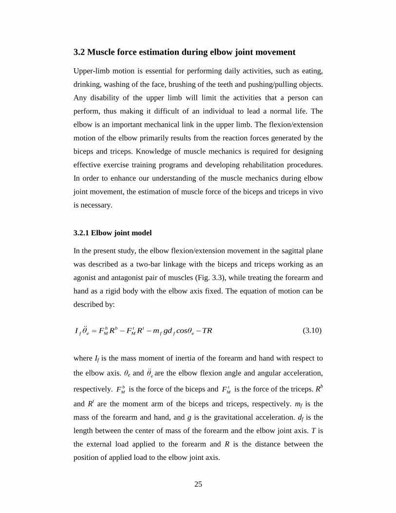
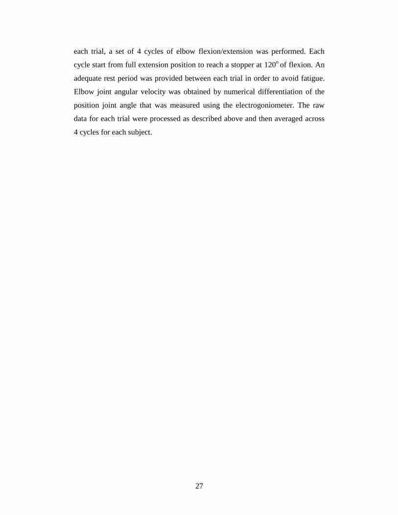
3.2.1 Elbow joint model
In the present study, the elbow flexion/extension movement in the sagittal plane
was described as a two-bar linkage with the biceps and triceps working as an
agonist and antagonist pair of muscles (Fig. 3.3), while treating the forearm and
hand as a rigid body with the elbow axis fixed. The equation of motion can be
described by:
TRcosθgdmRFRFθI eff
tt
M
bb
Mef (3.10)
where If is the mass moment of inertia of the forearm and hand with respect to
the elbow axis. θe and eθ are the elbow flexion angle and angular acceleration,
respectively. b
MF is the force of the biceps and t
MF is the force of the triceps. Rb
and Rt are the moment arm of the biceps and triceps, respectively. mf is the
mass of the forearm and hand, and g is the gravitational acceleration. df is the
length between the center of mass of the forearm and the elbow joint axis. T is
the external load applied to the forearm and R is the distance between the
position of applied load to the elbow joint axis.
Page 31
26
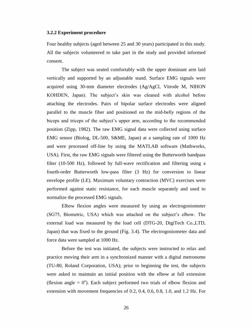
3.2.2 Experiment procedure
Four healthy subjects (aged between 25 and 30 years) participated in this study.
All the subjects volunteered to take part in the study and provided informed
consent.
The subject was seated comfortably with the upper dominant arm laid
vertically and supported by an adjustable stand. Surface EMG signals were
acquired using 30-mm diameter electrodes (Ag/AgCl, Vitrode M, NIHON
KOHDEN, Japan). The subject’s skin was cleaned with alcohol before
attaching the electrodes. Pairs of bipolar surface electrodes were aligned
parallel to the muscle fiber and positioned on the mid-belly regions of the
biceps and triceps of the subject’s upper arm, according to the recommended
position (Zipp, 1982). The raw EMG signal data were collected using surface
EMG sensor (Biolog, DL-500, S&ME, Japan) at a sampling rate of 1000 Hz
and were processed off-line by using the MATLAB software (Mathworks,
USA). First, the raw EMG signals were filtered using the Butterworth bandpass
filter (10-500 Hz), followed by full-wave rectification and filtering using a
fourth-order Butterworth low-pass filter (3 Hz) for conversion to linear
envelope profile (LE). Maximum voluntary contraction (MVC) exercises were
performed against static resistance, for each muscle separately and used to
normalize the processed EMG signals.
Elbow flexion angles were measured by using an electrogoniometer
(SG75, Biometric, USA) which was attached on the subject’s elbow. The
external load was measured by the load cell (DTG-20, DigiTech Co.,LTD,
Japan) that was fixed to the ground (Fig. 3.4). The electrogoniometer data and
force data were sampled at 1000 Hz.
Before the test was initiated, the subjects were instructed to relax and
practice moving their arm in a synchronized manner with a digital metronome
(TU-80, Roland Corporation, USA); prior to beginning the test, the subjects
were asked to maintain an initial position with the elbow at full extension
(flexion angle = 0o). Each subject performed two trials of elbow flexion and
extension with movement frequencies of 0.2, 0.4, 0.6, 0.8, 1.0, and 1.2 Hz. For
Page 32
27
each trial, a set of 4 cycles of elbow flexion/extension was performed. Each
cycle start from full extension position to reach a stopper at 120o
of flexion. An
adequate rest period was provided between each trial in order to avoid fatigue.
Elbow joint angular velocity was obtained by numerical differentiation of the
position joint angle that was measured using the electrogoniometer. The raw
data for each trial were processed as described above and then averaged across
4 cycles for each subject.
Page 33
28
Figure 3.3 A schematic of a simple two-bar linkage model represents the arm
with the biceps and triceps working as an agonist and antagonist pair of
muscles.
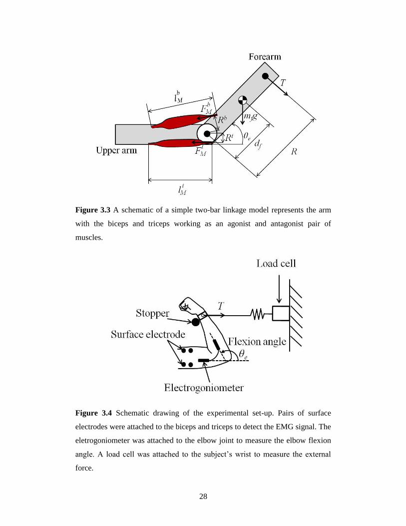
Figure 3.4 Schematic drawing of the experimental set-up. Pairs of surface
electrodes were attached to the biceps and triceps to detect the EMG signal. The
eletrogoniometer was attached to the elbow joint to measure the elbow flexion
angle. A load cell was attached to the subject’s wrist to measure the external
force.
Page 34
29
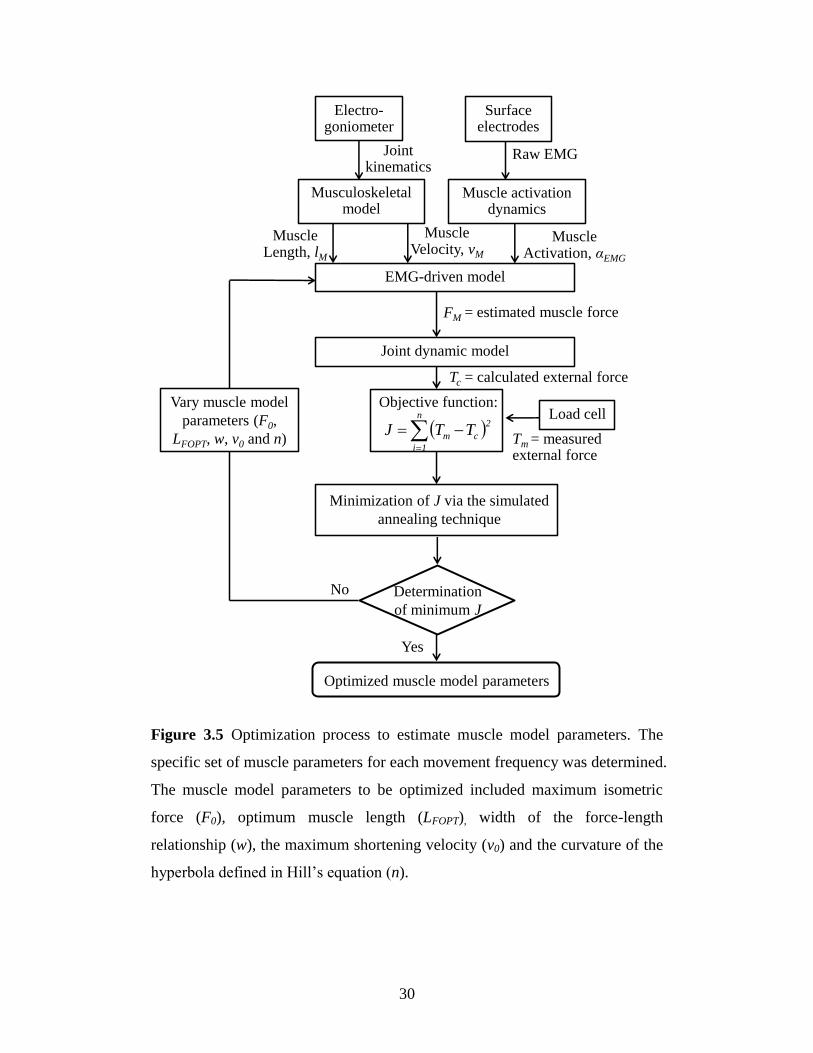
3.2.3 Optimization process
From the muscle model (Fig 3.1), the muscle model parameters to be optimized
included F0, LFOPT, w, v0 and n. The specific set of muscle parameters for each
movement condition was determined using an optimization method (Fig. 3.5).
We have assumed that the external force applied to the body’s limb estimated
by the model should match those measured from the load cell. A simulated
annealing algorithm was used to tune the model parameters by minimizing the
objective function, (J) given by:
n
1
2
cm TTJ (3.11)
where n is the number of samples during the entire movement in each trial, Tm
is the measured external force from the load cell and Tc is the estimated external
force calculated from the model. The initial estimation of the muscle parameters
was based on literature data (An, et al., 1981; Winters and Stark, 1985; Murray,
et al., 2000; Hale, et al., 2011), and the values were allowed to vary within the
physiological range. The optimization was calculated using the Optimization
Toolbox in MATLAB (Mathworks, USA).
Page 35
30
Figure 3.5 Optimization process to estimate muscle model parameters. The
specific set of muscle parameters for each movement frequency was determined.
The muscle model parameters to be optimized included maximum isometric
force (F0), optimum muscle length (LFOPT), width of the force-length
relationship (w), the maximum shortening velocity (v0) and the curvature of the
hyperbola defined in Hill’s equation (n).
Electro-goniometer
Musculoskeletal model
Joint kinematics
Muscle Length, lM
Muscle Velocity, vM
EMG-driven model
Surface electrodes
Muscle activation dynamics
Raw EMG
Muscle Activation, αEMG
Joint dynamic model
n
1i
2
cm TTJ
No
Yes
Vary muscle model
parameters (F0,
LFOPT, w, v0 and n)
Load cell
= estimated muscle force
Optimized muscle model parameters
Tc = calculated external force
Tm = measured external force
Objective function:
Minimization of J via the simulated
annealing technique
Determination
of minimum J
FM
Page 36
31
3.2.4 Results
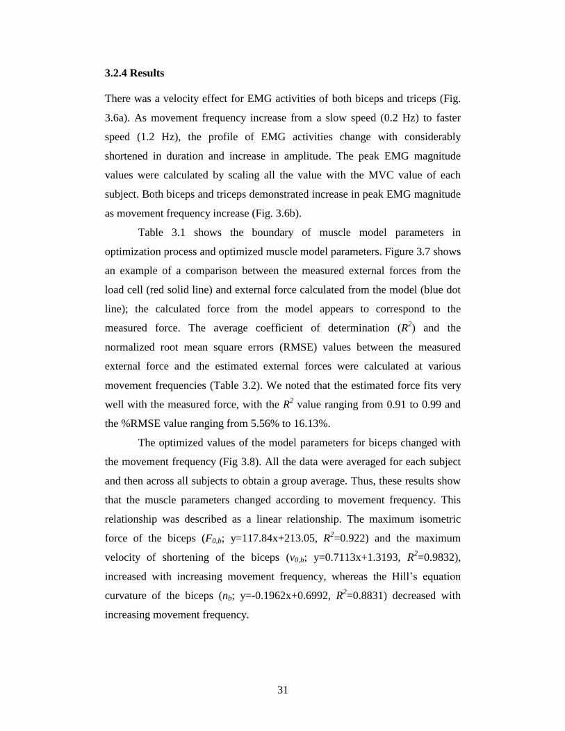
There was a velocity effect for EMG activities of both biceps and triceps (Fig.
3.6a). As movement frequency increase from a slow speed (0.2 Hz) to faster
speed (1.2 Hz), the profile of EMG activities change with considerably
shortened in duration and increase in amplitude. The peak EMG magnitude
values were calculated by scaling all the value with the MVC value of each
subject. Both biceps and triceps demonstrated increase in peak EMG magnitude
as movement frequency increase (Fig. 3.6b).
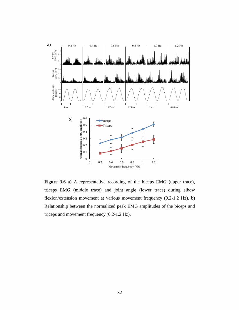
Table 3.1 shows the boundary of muscle model parameters in
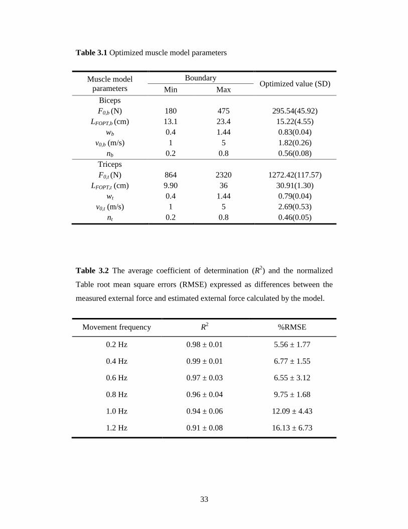
optimization process and optimized muscle model parameters. Figure 3.7 shows
an example of a comparison between the measured external forces from the
load cell (red solid line) and external force calculated from the model (blue dot
line); the calculated force from the model appears to correspond to the
measured force. The average coefficient of determination (R2) and the
normalized root mean square errors (RMSE) values between the measured
external force and the estimated external forces were calculated at various
movement frequencies (Table 3.2). We noted that the estimated force fits very
well with the measured force, with the R2 value ranging from 0.91 to 0.99 and
the %RMSE value ranging from 5.56% to 16.13%.
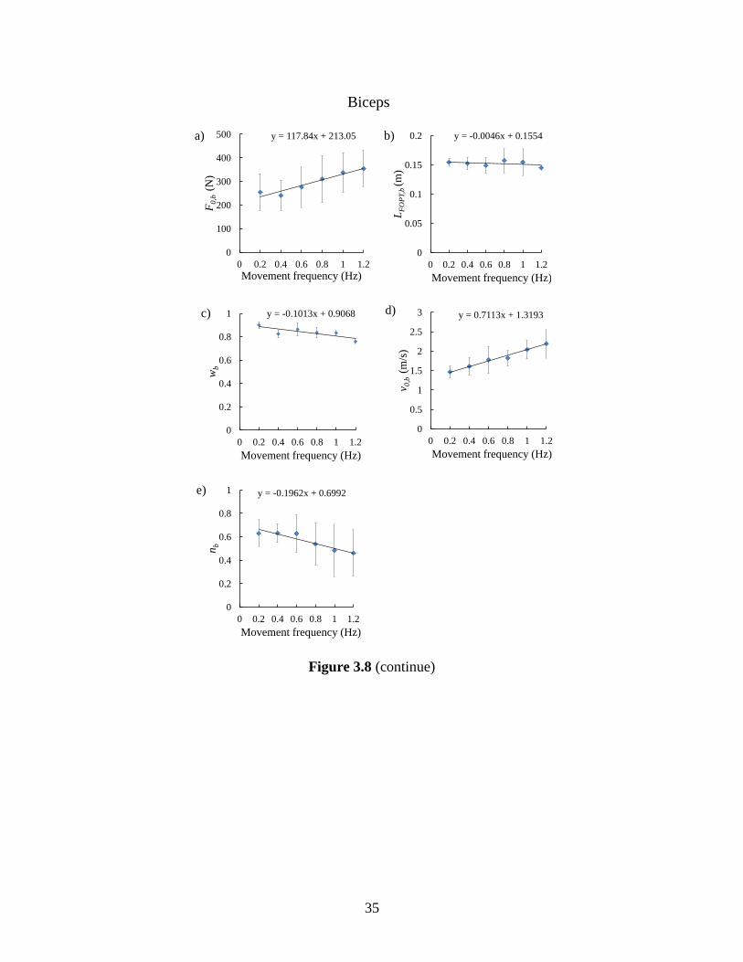
The optimized values of the model parameters for biceps changed with
the movement frequency (Fig 3.8). All the data were averaged for each subject
and then across all subjects to obtain a group average. Thus, these results show
that the muscle parameters changed according to movement frequency. This
relationship was described as a linear relationship. The maximum isometric
force of the biceps (F0,b; y=117.84x+213.05, R2=0.922) and the maximum
velocity of shortening of the biceps (v0,b; y=0.7113x+1.3193, R2=0.9832),
increased with increasing movement frequency, whereas the Hill’s equation
curvature of the biceps (nb; y=-0.1962x+0.6992, R2=0.8831) decreased with
increasing movement frequency.
Page 37
32
Figure 3.6 a) A representative recording of the biceps EMG (upper trace),
triceps EMG (middle trace) and joint angle (lower trace) during elbow
flexion/extension movement at various movement frequency (0.2-1.2 Hz). b)
Relationship between the normalized peak EMG amplitudes of the biceps and
triceps and movement frequency (0.2-1.2 Hz).
Bic
eps
EM
G (
mV
)
5 sec 2.5 sec 1.67 sec 1.25 sec 1 sec 0.83 sec
Tri
cep
s
EM
G (
mV
)
Elb
ow
join
t an
gle
(deg
ree)
0.2 Hz 0.4 Hz 0.6 Hz 0.8 Hz 1.0 Hz 1.2 Hz
0
0.1
0.2
0.3
0.4
0.5
0.6
0 0.2 0.4 0.6 0.8 1 1.2
No
rmal
ized
pea
k E
MG
am
pli
tud
e
Movement frequency (Hz)
Biceps
Triceps
a)
b)
Page 38
33
Table 3.1 Optimized muscle model parameters
Table 3.2 The average coefficient of determination (R2) and the normalized
Table root mean square errors (RMSE) expressed as differences between the
measured external force and estimated external force calculated by the model.
Movement frequency R2
%RMSE
0.2 Hz 0.98 ± 0.01 5.56 ± 1.77
0.4 Hz 0.99 ± 0.01 6.77 ± 1.55
0.6 Hz 0.97 ± 0.03 6.55 ± 3.12
0.8 Hz 0.96 ± 0.04 9.75 ± 1.68
1.0 Hz 0.94 ± 0.06 12.09 ± 4.43
1.2 Hz 0.91 ± 0.08 16.13 ± 6.73
Muscle model
parameters
Boundary Optimized value (SD)
Min Max
Biceps
F0,b (N)
LFOPT,b (cm)
wb
v0,b (m/s)
nb
180
13.1
0.4
1
0.2
475
23.4
1.44
5
0.8
295.54(45.92)
15.22(4.55)
0.83(0.04)
1.82(0.26)
0.56(0.08)
Triceps
F0,t (N)
LFOPT,t (cm)
wt
v0,t (m/s)
nt
864
9.90
0.4
1
0.2
2320
36
1.44
5
0.8
1272.42(117.57)
30.91(1.30)
0.79(0.04)
2.69(0.53)
0.46(0.05)
Page 39
34
Figure 3.7 An example of comparison of the external force, T between
measured force (red solid line) and estimated external force calculated from the
model (blue dot line) in a) movement frequency 0.2 Hz and b) movement
frequency 1.2 Hz.
Page 40
35
Figure 3.8 (continue)
y = 117.84x + 213.05
0
100
200
300
400
500
0 0.2 0.4 0.6 0.8 1 1.2
F0,b
(N
)
Movement frequency (Hz)
a) y = -0.0046x + 0.1554
0
0.05
0.1
0.15
0.2
0 0.2 0.4 0.6 0.8 1 1.2
LF
OP
T,b
(m)
Movement frequency (Hz)
b)
y = 0.7113x + 1.3193
0
0.5
1
1.5
2
2.5
3
0 0.2 0.4 0.6 0.8 1 1.2
v 0,b
(m/s
)
Movement frequency (Hz)
d)
y = -0.1962x + 0.6992
0
0.2
0.4
0.6
0.8
1
0 0.2 0.4 0.6 0.8 1 1.2
nb
Movement frequency (Hz)
e)
y = -0.1013x + 0.9068
0
0.2
0.4
0.6
0.8
1
0 0.2 0.4 0.6 0.8 1 1.2
wb
Movement frequency (Hz)
c)
Biceps
Page 41
36
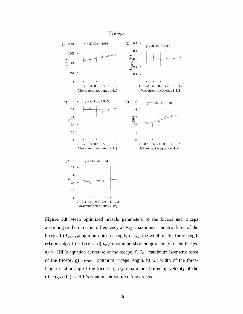
Figure 3.8 Mean optimized muscle parameters of the biceps and triceps
according to the movement frequency a) F0,b: maximum isometric force of the
biceps, b) LFOPT,b: optimum biceps length, c) wb: the width of the force-length
relationship of the biceps, d) v0,b: maximum shortening velocity of the biceps,
e) nb: Hill’s equation curvature of the biceps. f) F0,t: maximum isometric force
of the triceps, g) LFOPT,t: optimum triceps length, h) wt: width of the force-
length relationship of the triceps, i) v0,t: maximum shortening velocity of the
triceps, and j) nt: Hill’s equation curvature of the triceps.
y = 294.9x + 1066
0
500
1000
1500
2000
0 0.2 0.4 0.6 0.8 1 1.2
F0,t
(N
)
Movement frequency (Hz)
f)y = -0.0016x + 0.3103
0
0.1
0.2
0.3
0.4
0.5
0 0.2 0.4 0.6 0.8 1 1.2
LF
OP
T,t
(m)
Movement frequency (Hz)
g)
y = -0.011x + 0.795
0
0.2
0.4
0.6
0.8
1
0 0.2 0.4 0.6 0.8 1 1.2
wt
Movement frequency (Hz)
h) y = 1.2603x + 1.803
0
1
2
3
4
5
0 0.2 0.4 0.6 0.8 1 1.2
v 0,t
(m
/s)
Movement frequency (Hz)
i)
y = 0.0704x + 0.4061
0
0.2
0.4
0.6
0.8
1
0 0.2 0.4 0.6 0.8 1 1.2
nt
Movement frequency (Hz)
j)
Triceps
Page 42
37
Figure 3.9 (continue)
Page 43
38
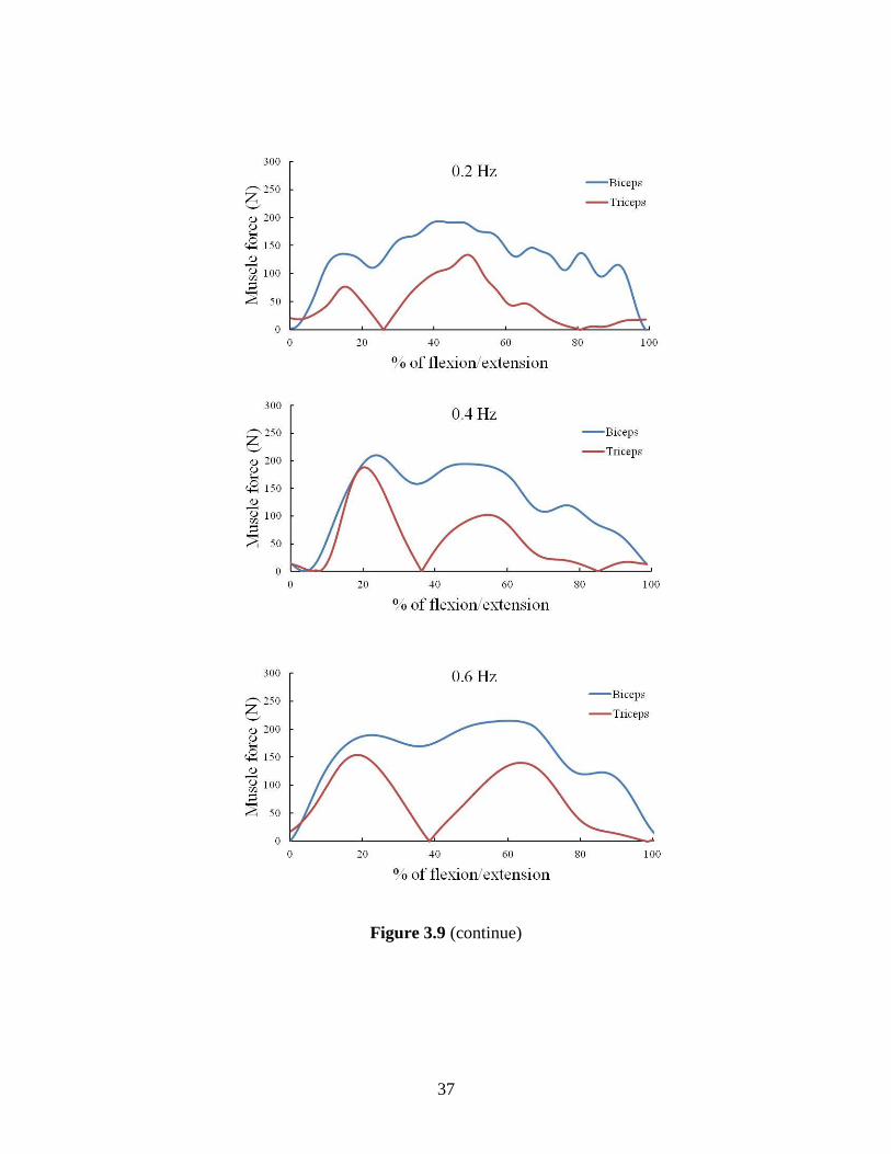
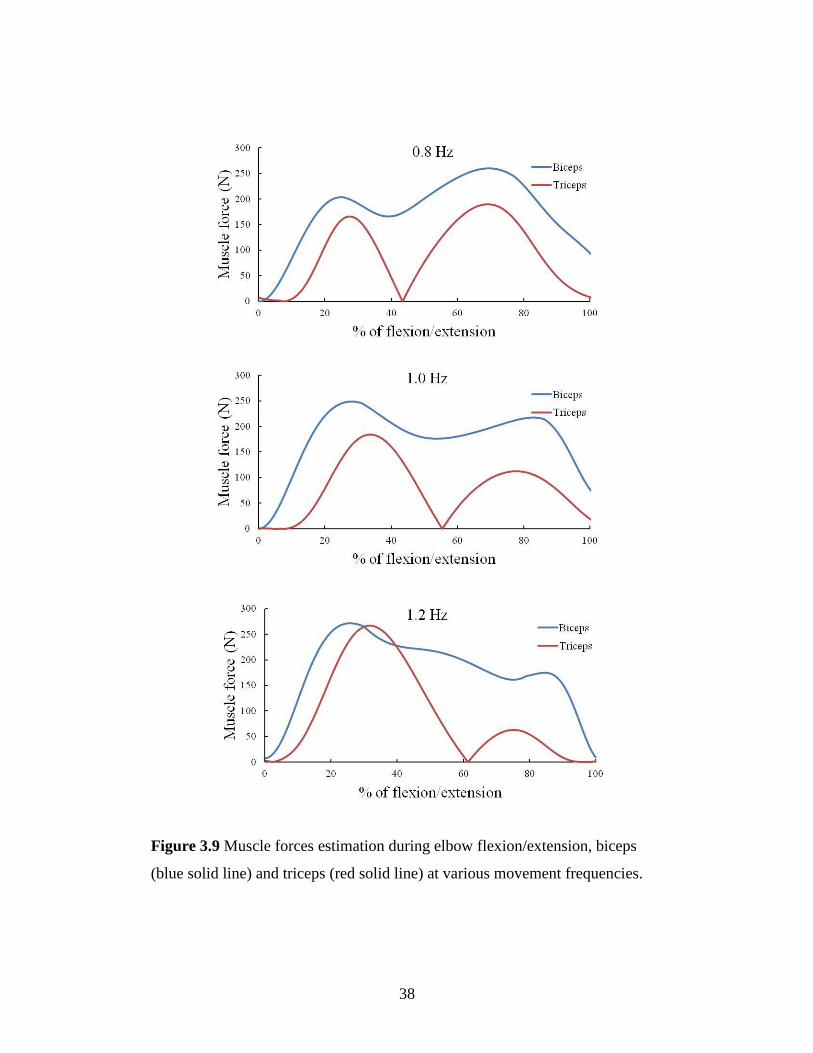
Figure 3.9 Muscle forces estimation during elbow flexion/extension, biceps
(blue solid line) and triceps (red solid line) at various movement frequencies.
Page 44
39
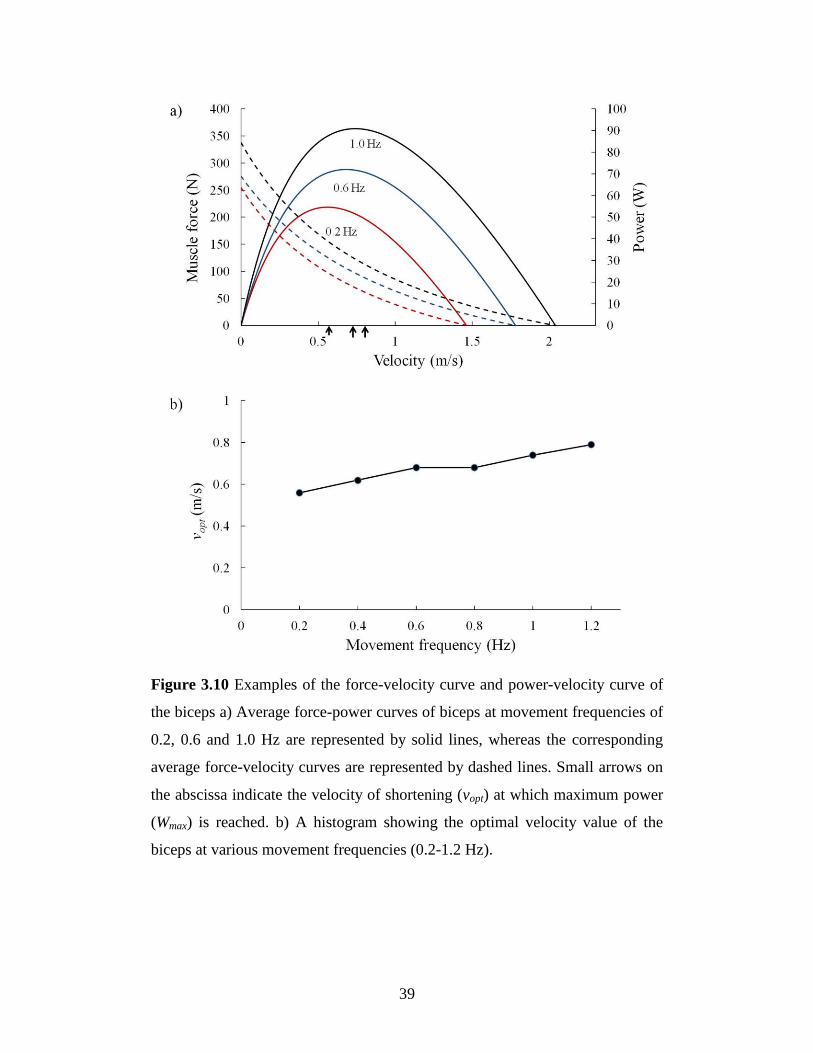
Figure 3.10 Examples of the force-velocity curve and power-velocity curve of
the biceps a) Average force-power curves of biceps at movement frequencies of
0.2, 0.6 and 1.0 Hz are represented by solid lines, whereas the corresponding
average force-velocity curves are represented by dashed lines. Small arrows on
the abscissa indicate the velocity of shortening (vopt) at which maximum power
(Wmax) is reached. b) A histogram showing the optimal velocity value of the
biceps at various movement frequencies (0.2-1.2 Hz).
Page 45
40
however, the optimum biceps length (LFOPT,b;y=-0.0046x+0.1554, R2=0.1433)
and the width of the force-length relationship of the biceps (wb;y=-
0.1013x+0.9068, R2=0.6541) changed minimally with increasing movement
frequency. The optimized model parameters for the triceps also changed with
the movement frequency. The relationship was also described as a linear
relationship; The maximum isometric force of the triceps (F0,t;y=294.9x+1066,
R2=0.882), and the maximum velocity of shortening of the triceps (v0,t;
y=1.2603x+1.803, R2=0.796) increased with increasing movement frequency,
whereas there was minimal change in the optimal triceps length (LFOPT,t;y=-
0.0016x+0.3103, R2=0.002), width of the force-length relationship, (wt; y=-
0.011x+0.795, R2=0.0099), and Hill’s equation curvature of the triceps (nt;
y=0.0704x+0.4061, R2=0.3248) with increasing movement frequency.
Biceps and triceps forces were estimated during elbow flexion/motion at
various moving speeds (Fig. 3.9). The muscle contributions changed during the
motion. The muscle force of the biceps and triceps increased as movements
frequencies increased. The change in biceps and triceps force pattern can be
observed at every movement frequencies.
The average power-velocity curves were calculated using the
information from the force-velocity curve. As noted in Fig. 3.10a, the muscle
can generate greater maximum power output (Wmax) at a higher movement
frequency. The optimal velocity (vopt), where Wmax is reached is shown in Fig.
3.10b. Moreover, the vopt value increases as the movement frequency increases.
Page 46
41
3.2.5 Discussion
In this study, an EMG-driven model was developed and used to estimate
muscle force during elbow flexion/extension movement. The optimization
process used data from various movement frequencies. The change in muscle
force contribution can be observed non-invasively.
During elbow flexion/extension movement, both biceps and triceps
generate force to move forearm as shown in Fig. 3.9. Level and timing of
muscle force generation change with movement speed. As movement speed
increase more force is required to generate faster movement. During flexion (0-
50% of flexion/extension movement), biceps works as agonist muscle and
triceps works as antagonist muscle. While during extension (50-100% of
flexion/extension) triceps work as agonist and biceps works as antagonist
muscle. The results seem consistent with the anatomical information. The
cooperative activity of biceps and triceps was presented. The pattern seems
similar in every movement speed (Fig. 3.9). The maximum biceps force occur
at about 20% of flexion/extension cycle which required to move forearm and
the maximum triceps force occur later at about 40% of flexion/extension cycle
to break the forearm movement.
Another finding of the present study is that muscle model parameters
depend on the movement frequency. The impact of the rate-effect on the muscle
parameters is shown in Fig. 3.8. When the forearm moves with a higher
movement frequency, greater power is required to generate the movement. The
change in shortening velocity of muscle directly affects the operating point in
the force-velocity relationship. The force-velocity relationship dictates that a
muscle’s ability to produce force decrease with increasing speeds of
contraction, and hence there is an optimum shortening velocity which maximal
power is produced. It is well known fact that human muscle is non-
homogeneous, and is composed of two muscle fiber types, type I (slow) and
type II (fast), which have different roles and properties (Close, 1972). Both
fiber types contribute to muscle force generation during muscle contraction.
The properties of muscles might change according to the movement velocity of
Page 47
42
the task, since muscles tend to operate in vivo at a velocity and load condition
at which maximum power is developed (Rome, et al., 1988). The recruitment
strategy of both muscle fibers during dynamic contraction is not yet fully
understands due to the limitation of conducting in vivo experiment in human.
However, Rome et al. (1988) demonstrated that in carp, fast and slow fibers
shorten at different velocities which develops their maximum power output.
This indicates that there is a mechanism to optimize mechanical power and
efficiency at different movement speeds by selective recruitment of the suitable
fiber type. Assuming that the same mechanism also holds true in human, the
muscle tends to operate at a point of optimum velocity where speed and power
are most efficiently utilized. We noted that the F0 and v0 values increased with
higher movement frequency. An increase in the F0 and v0 values in the force-
velocity relationship facilitates the generation of greater maximum power
output (Wmax) in the muscle (Fig. 3.10a). The F0 and v0 values depend on the
muscle fiber composition since the properties of the entire muscle lump is
determined by the properties values of the combined fast fibers and slow fibers
(Zajac, 1989). Both fiber types contribute to muscle force generation during
muscle contraction. Properties of the whole muscle lump during contraction can
be changed depend on the recruitment of both slow and fast fibers. Walmsley et
al. (1978) shown that during locomotion in cat, over a wide range of walking
speeds (0.6–3 m/s), soleus (100% slow muscle fibers) developed approximately
the same peak force while the average medial gastrocnemius (mixed muscle
fibers) force varies over a threefold range. Many studies report that fast fibers
have higher F0 and v0 values as compared to slow fibers (Larsson and Moss,
1993; Harridge, et al., 1996; Bottinelli, et al., 1999). In addition the change in
F0 could be regarded to be proportional to change in maximum muscle stress
(σm). Many studies in cat and human muscle reported that the value of σm in fast
fiber is higher than in slow fiber (Burke, et al., 1973; Dum, et al., 1982; Bodine,
et al., 1987; Bottinelli, et al., 1996). At a higher speed, fast fibers play an
important role in generating force, since fast fibers can produce much greater
power as compared to slow fibers (Bottinelli, et al., 1999). In addition, at high
Page 48
43
movement frequency, the velocities at which the muscle shortens can be faster
than the v0 of its slow fiber. Therefore, when the shortening velocity increases,
the properties of the entire muscle lump should shift toward and reflect the
values of the fast fibers. An increase in the F0 and v0 values also facilitates the
generation of optimum power output at a higher shortening velocity in the
muscle. The change in the vopt (Fig. 3.10b) indicates that during dynamic
contraction, the muscle tends to tune its properties to extent at which the muscle
can work efficiently. Therefore, varying the F0 and v0 values with the
movement frequency enable to better reflect the underlying mechanism in the
muscle. At first a simple linear relation between these parameters and
movement frequency can be implemented. The relationship can be extracted
from the results of this study (Fig. 3.8).
In the force-length relationship, the parameters that describe the
relationship are the LFOPT (defined as the muscle length at which the muscle
generates maximum force) and w. The results show that both LFOPT and w
slightly changed with increasing movement frequency. The effective operating
range of muscle is approximately between 0.5LFOPT and 1.5LFOPT (Zajac, 1989)
(w 1). Many studies report operating range of muscle in ascending or plateau
region of the force-length curve (Loren, et al., 1996; Murray, et al., 2000; Hale,
et al., 2011). It seems that slightly change in these parameters does not have
much effect on this region of force-length curve. Muscle still operates at the
optimum point at which the muscles work most efficiently in the force-length
relationship. Thus, the impact of the rate-effect on these parameters appears to
be minimal.
In order to improve the accuracy of the EMG-driven model when using
in a wide range of speed movement, muscle model parameters should be
adjusted according to the movement speed. Muscle model parameters should be
tuned at the slowest and fastest movement condition to form a linear
relationship.
A limitation encountered when developing an EMG-driven model is that
the muscle force cannot be measured directly. To evaluate the accuracy of the
Page 49
44
estimated muscle force, it is necessary to compare the calculated external force
with the measured force. The accuracy of the estimated muscle force depends
on the proposed mechanical model. The lumped model being used in the
present study consists of the combination, of all of the elbow flexors as a single
“biceps” and all the extensors as a single “triceps” (Bouisset, 1973; Winters and
Stark, 1985). This basic approach of lumping synergistic muscles is useful
when assessing tasks involving motion of a single joint such as the elbow joint.
However, it should be noted that there are more than two muscles at every joint.
For studies of certain specific tasks, separation of synergistic muscles is
necessary. By adding more muscle models into the mechanical model, we can
study a system that exhibits a wide range of human movement.
In present study, there are five muscle model parameters to be adjusted.
These parameters are enough for describing the mechanism of the force-length-
velocity relationship. Adding more muscle model parameters to be optimized
might help in fit more between the estimated force and measured force.
However, this should be carefully performed as the added complexity can make
interpretation of results more difficult. Buchanan et al. (2004) suggested that
the fewer optimization variables that are adjusted, the more assured the
physiological meaning of the model. Good agreement between the external
forces calculated from the model and the measured ones (Fig. 3.7) showed the
feasibility of this approach to estimate muscle model parameters.
The EMG signals recorded with surface electrodes is dependent on
several factors, such as skin thickness, the distance of the electrode from the
active muscle area, and the quality of contact between the electrode and skin.
The EMG signals from the muscles that are near the skin surface, such as the
biceps and triceps, can be easily measured. However, we did not succeed in
obtaining a stable isolated EMG signals from the branchialis muscle because it
is deeply located under the biceps. Thus, if the brachialis muscle with
inaccurate EMG signal is included into the mechanical model, a significant
error may be obtained. Therefore, we did not include the brachialis in our
model.
Page 50
45
Increase in the movement frequency affects the accuracy of the
estimated muscle force of the Hill-type muscle model. In the present study, we
noted that the model estimated the force with good accuracy (%RMSE<10%)
within a range of 0.2-0.8 Hz, which is the range of normal movement. The error
of the estimated force increased with higher movement frequency (at 1.0 and
1.2 Hz.). This limitation may be attributed to the lack of the force-acceleration
relationship in the CE. The Hill’s muscle model is generally based on the force-
velocity relationship in isotonic contractions, and thus it appears to be suitable
for slow movements with constant force. However, during rapid movement, the
force generated rapidly by muscle changes during the acceleration phase, may
induce an error in Hill’s muscle model. Moreover, the force acceleration
relationship in such cases is not well known. Certain studies have indicated that
muscle respond differently to all three kinematic parameters, including velocity,
acceleration and jerk (Le Bozec, et al., 1987; Fee Jr, et al., 2009). Thus, we
believe that a better understanding of the force-acceleration relationship in vivo
could be useful for developing an EMG-driven model for rapid movement.
For accurately estimating muscle force using the EMG-driven model,
the change in the muscle model parameters according to movement frequency
should be considered. The EMG-driven model with adjusted muscle model
parameters is effective in estimating the muscle force during normal
movements (frequency: 0.2-0.8 Hz). To further improve the muscle model, we
suggest that the relationship between acceleration and muscle force should be
investigated and this should be included into the muscle model.
Page 51
46
3.3 Muscle force estimation during knee joint movement
Knee motion is required during most of daily activities, such as walking,
ascending/descending stairs, cycling and sitting up/down. Human knee has an
ability to move in various speeds by adjusting muscle force that generated from
each muscle within the lower limb. The ability to adjust the speed is an
important mechanism that provides adaptation to change in locomotion activity,
e.g. change from walking to running or to enhance stability during the
movement. The evaluation of the muscle force at knee joint is of importance in
many areas of biomechanics research such as improving rehabilitation program,
design of better implant systems and development of training program for
athletes. However, direct measurement of muscle force is difficult and invasive,
thus indirect measurement and mathematical model is required to estimate the
muscle force. Many study developed an inverse dynamics model to estimate
joint moment from external forces and kinematics of body movement (Kingma,
et al., 1996; Silva and Ambrósio, 2002; Erdemir, et al., 2007). Many studies
reported the change in EMG activities of several muscles in lower limbs when
movement speed increase (Hwang and Abraham, 2001; Hof, et al., 2002; den
Otter, et al., 2004). Understanding muscular contributions to knee
flexion/extension is of important in studying muscle mechanism and developing
a better rehabilitation program. Therefore, we were interested in determining
how individual muscles contribute to knee flexion/extension when the
movement speed change using EMG-driven model.
Page 52
47
3.3.1 Knee joint model
The knee flexion/extension movement in the sagittal plane was described by a
segmental model where the shank and thigh were considered to be two rigid
bodies, connected by a hinge-type joint, as shown in Fig. 3.11. The model
considered the rectus femoris (RF), vatsus lateralis (VL), biceps femoris (BF)
and gastrocnemius (GaS) muscles. These muscles generate forces that drive the
knee joint to move. The equation of motion can be described by
sskssextensorextensorflexorflexorks RTcosθgdmRF-RFθI (3.12)
where Is is the mass moment of inertia of the shank and foot with respect to the
knee axis. θk and kθ are the knee flexion angle and angular acceleration,
respectively. Fflexor is the force of the flexors, and Fextensor is the force of the
extensors. Rflexor and Rextensor are the moment arms of the flexors and extensors
respectively. ms is the mass of the shank and foot. ds is the length between the
center of mass of the shank, and the knee joint axis. Ts is the external load
applied to the shank, and Rs is the distance between the position of the applied
load to the knee joint axis.
Page 53
48
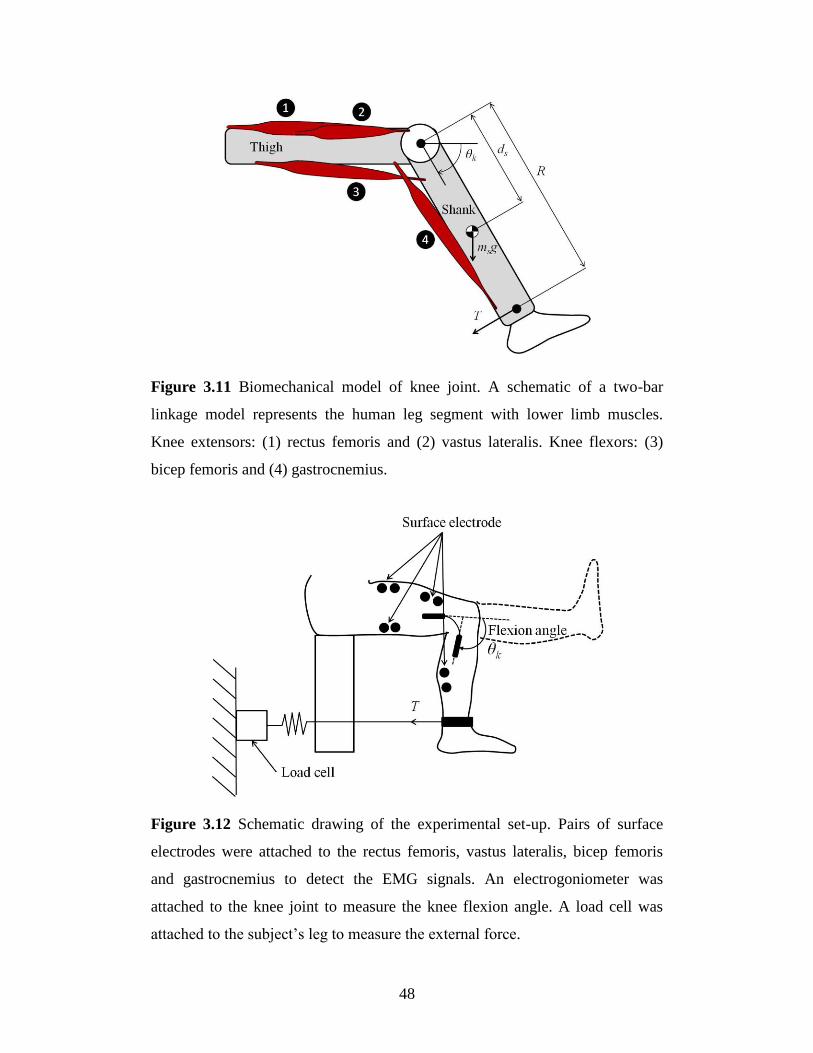
Figure 3.11 Biomechanical model of knee joint. A schematic of a two-bar
linkage model represents the human leg segment with lower limb muscles.
Knee extensors: (1) rectus femoris and (2) vastus lateralis. Knee flexors: (3)
bicep femoris and (4) gastrocnemius.
Figure 3.12 Schematic drawing of the experimental set-up. Pairs of surface
electrodes were attached to the rectus femoris, vastus lateralis, bicep femoris
and gastrocnemius to detect the EMG signals. An electrogoniometer was
attached to the knee joint to measure the knee flexion angle. A load cell was
attached to the subject’s leg to measure the external force.
Page 54
49
3.3.2 Experiment procedure
Two healthy subjects participated in this study. The subjects sat comfortably in
an upright position and performed a series of knee joint flexion and extension
movements with predetermined movement frequencies ranging from 0.2 Hz to
1.0 Hz. Knee flexion angles were measured with an electrogoniometer (SG75,
Biometric, USA) that was attached to the subject’s leg. The external load was
measured by a load cell (DTG-20, DigiTech Co.,Ltd., Japan) that was fixed to
the ground (Fig. 3.12). The raw EMG signals from the RF, VL, BF and GaS
were collected with bipolar surface electrodes at a sampling rate of 1000 Hz
(Biolog, DL-500, S&ME, Japan) and processed offline with the MATLAB
software (Mathworks, USA). First, the raw EMG signals were filtered using the
Butterworth bandpass filter (10-500 Hz); this was followed by full-wave
rectification and filtering using a fourth-order Butterworth low-pass filter (3
Hz) for conversion to a linear envelope profile. MVC exercises were performed
against static resistance for each muscle separately in order to normalize the
processed EMG signals.
Before the test was initiated, the subjects were instructed to relax and
practice moving their leg in a synchronized manner with a digital metronome
(TU-80, Roland Corporation, USA). Each subject performed two trials of knee
flexion and extension with movement frequencies of 0.2, 0.4, 0.6, 0.8, and 1.0
Hz. For each trial, a set of 20 cycles of knee flexion/extension movements was
performed. The range of motion executed at the knee was between 0o and 90
o.
An adequate rest period was provided between each trial in order to avoid
fatigue. The knee joint angular velocity was obtained by numerical
differentiation of the position joint angle that was measured by the
electrogoniometer. The raw data for each trial were processed as described
above and then averaged across 20 cycles for each subject.
Page 55
50
3.3.3 Results
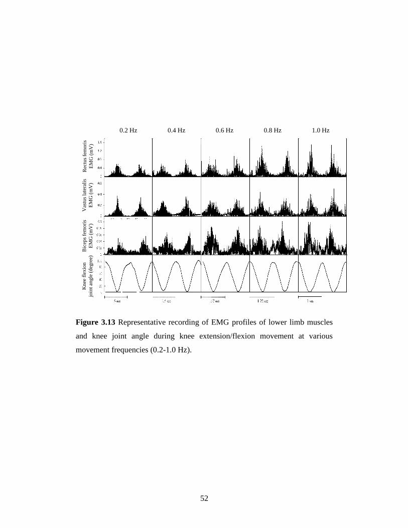
Figure 3.13 shows EMG recordings of the RF, VL, and BF muscles and the
knee flexion angle during extension/flexion. The amplitude and timing changed
when the movement speed increased. This shows the influence of the
movement speed on the muscle force generation mechanism. As the movement
frequency increased from a slow speed (0.2 Hz) to a faster speed (1.0 Hz), both
RF and BF EMG activities changed with a substantial decrease in duration and
increase in amplitude. The peak RF EMG activity appeared at full extension.
The peak BF EMG activity at low speed (0.2 Hz) appeared late in the
extension, and the timing and amplitude changed when the speed increased. In
contrast, changing the movement speed had little influence on the VL. The VL
EMG activity seemed comparatively stable when the movement speed
increased.
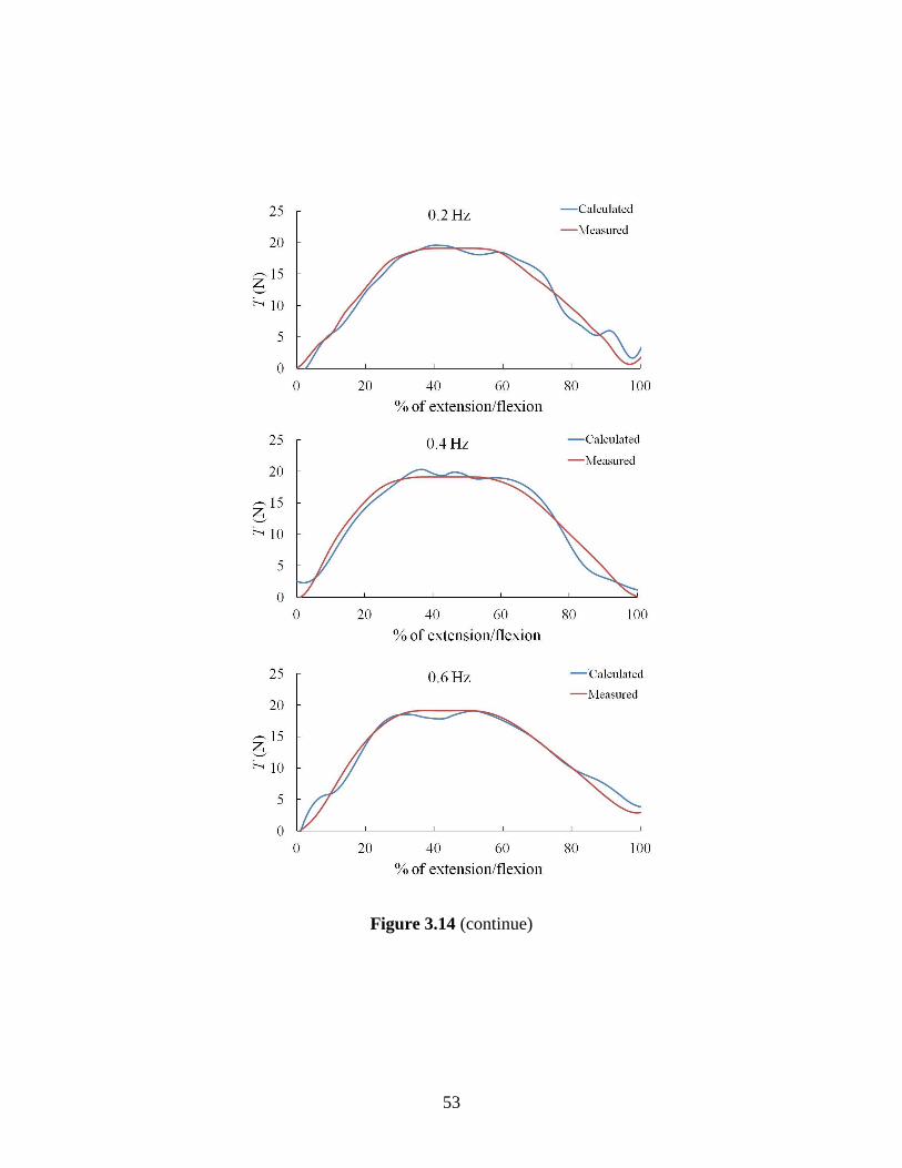
The muscle force of each muscle was estimated using EMG data and the
joint angle as inputs for the developed EMG-driven model. The predictive
ability of the model was validated by the fitness between the external forces
calculated by the inverse dynamic model and the measured values during the
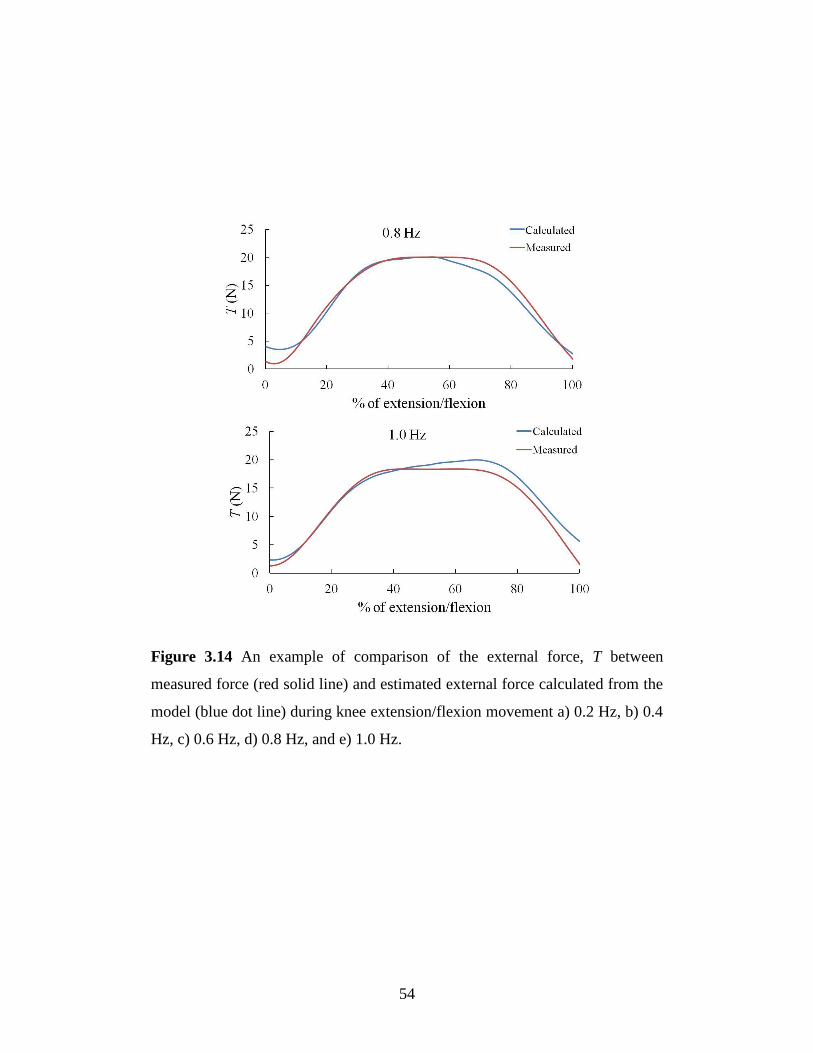
experimental trials. Figure 3.14 shows an example comparison between the
measured external forces from the load cell (red solid line) and external force
calculated from the model (blue dotted line); the calculated and measured
forces appear to correspond. The average coefficient of determination (R2) and
the predicted external forces were calculated at various movement frequencies.
The R2 values ranged from 0.91 to 0.97 and, the %RMSE ranged from 3.68% to
6.68%; thus, the predicted and measured forces showed good correspondence.
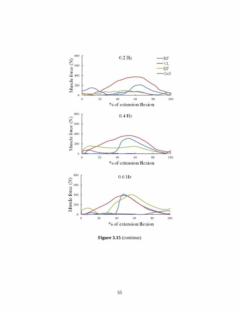
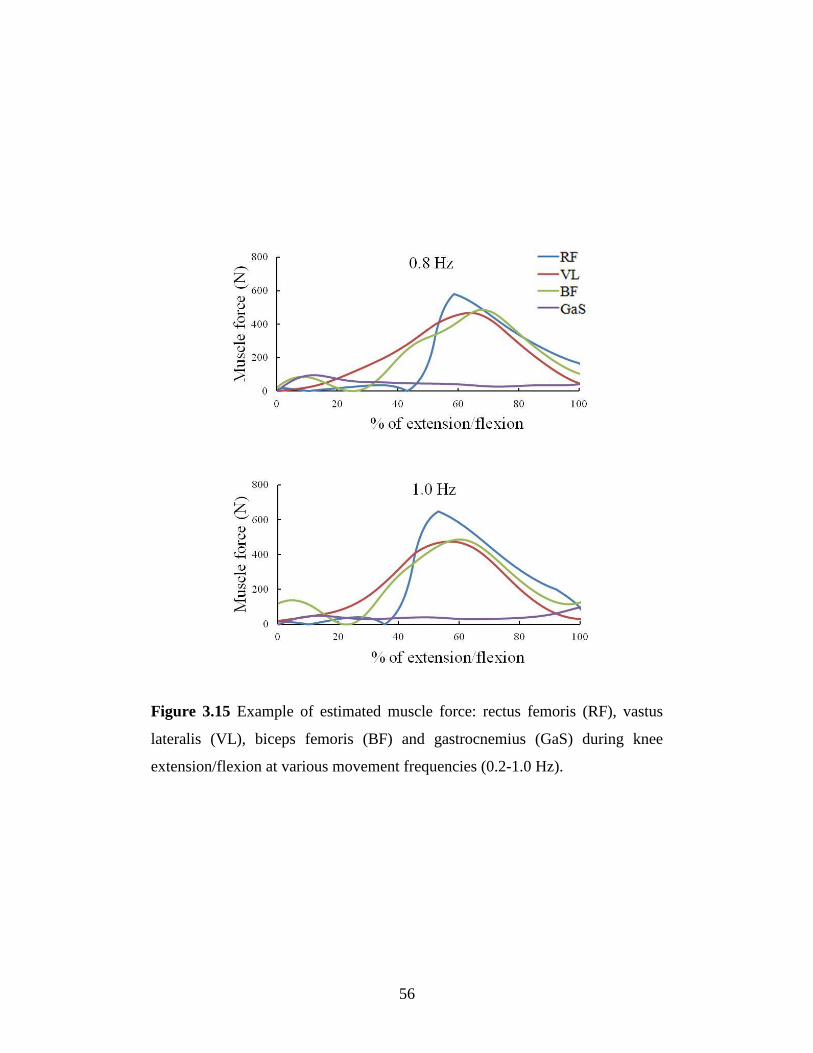
Individual muscle forces were estimated during knee flexion/motion at
various moving speeds (Fig. 3.15). The muscle contributions changed during
the motion. The muscle force of the VL showed a minimal change in muscle
force when the movement speed increased. In contrast, the RF and BF
generated more force when the movement speed increased. During slow
movement (e.g., 0.2 and 0.4 Hz), the VL was the main muscle that contributed
Page 56
51
to generating knee extension. For faster movements, the RF was the main
muscle that accelerated the body segment to achieve the desired speed. The
increased co-contraction of the RF and BF was observed at higher speeds (e.g.,
0.8 and 1.0 Hz). The peak force of the VL occurred at about 60% of the
extension/flexion time and stayed the same for all speeds. The GaS provided
only a small contribution during knee flexion/extension movements.
Page 57
52
Figure 3.13 Representative recording of EMG profiles of lower limb muscles
and knee joint angle during knee extension/flexion movement at various
movement frequencies (0.2-1.0 Hz).
0.2 Hz 0.4 Hz 0.6 Hz 0.8 Hz 1.0 Hz
Rec
tus
fem
ori
s
EM
G (
mV
)
Vas
tus
late
rali
s
EM
G (
mV
)
Bic
eps
fem
ori
s
EM
G (
mV
)
Kn
ee f
lexio
n
join
t an
gle
(d
egre
e)
Page 58
53
Figure 3.14 (continue)
Page 59
54
Figure 3.14 An example of comparison of the external force, T between
measured force (red solid line) and estimated external force calculated from the
model (blue dot line) during knee extension/flexion movement a) 0.2 Hz, b) 0.4
Hz, c) 0.6 Hz, d) 0.8 Hz, and e) 1.0 Hz.
Page 60
55
Figure 3.15 (continue)
Page 61
56
Figure 3.15 Example of estimated muscle force: rectus femoris (RF), vastus
lateralis (VL), biceps femoris (BF) and gastrocnemius (GaS) during knee
extension/flexion at various movement frequencies (0.2-1.0 Hz).
Page 62
57
3.3.4 Discussion
Figure 3.13 shows EMG activities during human knee flexion/extension under
different speed conditions. The EMG activity reflects the electrical state of a
contracting muscle and can be related to the muscle force. The changes in the
EMG signals show the influence of speed on the muscle mechanism. Each
muscle reacts to a change in speed differently. The EMG signals from the RF
and BF changed significantly when the movement speed increased. A marked
change appeared in the BF EMG initiation relative to the knee angle with the
phase advanced, which led to a co-contraction phase with the RF. The co-
contraction of the RF and BF increased with the movement speed. For repeated
cycling movements, Suzuki et al. (1982) reported on the changes in the RF and
BF activities as the pedaling speed increases. The movement speed seems to
have a strong influence on the RF and BF muscles. This may be due to the
increase in muscle co-contraction to increase stability and accelerate/decelerate
a body segment. Muscle co-contraction is the simultaneous activity of agonists
crossing the same joint and acts as a stabilizer (Busse, et al., 2005). Based on
the results, studying the timing of this co-contraction may help in developing
stability control of lower limbs.
Figure 3.15 shows individual muscle forces during knee
extension/flexion at different movement frequencies; the results provided
additional insight into how muscles react to changes in speed. The role of
muscles in knee extension/flexion motion is to control the accelerating and
decelerating forces of the shank segment. The amplitude of the muscle force
increases with the movement speed because of the need for a larger force
output. For low movement speeds (e.g., 0.2, 0.4, and 0.6 Hz), the VL is the
main muscle that generates the extension force and changes in the movement
speed seem to have a low influence on VL activity. During the braking phase
(50% extension/flexion time) at higher speeds, the RF generates more forces.
Many studies on muscle activity during walking have reported that the RF
activity increases with the walking speed (Shiavi, et al., 1987; Nene, et al.,
Page 63
58
1999; den Otter, et al., 2004). The results of this study confirm that the role of
RF is to accelerate the leg at higher movement speeds.
Some specific limitations of the presented technique and results must
also be addressed. In this study, the biomechanical model of the knee joint did
not consider the smaller muscles with small contributions to the total plantar
flexion torque. Several other muscles act synergistically for plantar flexion and
can be activated to stabilize the knee joint in the frontal plane. However, any
production should be based on muscle activity analysis for a given task. Since
these smaller muscles are deep, surface EMG access is difficult. Considering
more muscles may improve the model accuracy but the instability of EMG
signals from deep muscles should also be considered.
In this study, an EMG-driven model for predicting muscle forces in
lower limbs was developed and used to examine the contributions of individual
muscles to knee flexion/extension motion. The changes in muscle force when
the movement speed increased was observed and analyzed. This system
provides insight into muscle force generation during knee motion, which can
lead to better understanding of the muscle mechanisms and development of a
rehabilitation program.
Page 64
59
3.4 Summary
It was demonstrated that the developed EMG-driven model can be used to
estimate muscle force in elbow and knee joint during flexion/extension motion.
Body kinetic and EMG signals were used as inputs to the model. Individual
muscle force of each joint during dynamic movement was estimated. The
results show that there is the relationship between movement speed and EMG
signal. The EMG-driven model using conventional surface EMG is very useful
in estimating muscle force in elbow and knee joint which are moved by large
muscles. However, the limitations of conventional surface EMG signal to
access deep muscle, preventing the possibility of using this system to estimate
force in human forearm. To estimate muscle force within the forearm, the
development of a method to detect muscle activity in deep forearm muscle is
necessary.
Page 65
60
Chapter 4 An EMG-CT Method for
Detection of Multi Muscle Activity in the
Forearm
Page 66
61
4.1 EMG-CT method
The human hand is an excellent end-effector of the upper limb capable of
innumerable actions, from fine operations to heavy-duty tasks. A complex
movement of the hand is generated by the coordination of many muscles and
tendons in the forearm. There are 19 muscles reside within the human forearm.
List of forearm muscle is shown in Fig. 4.1 and Table 4.1. Mechanically, there
are four joints in each finger, from the proximal to distal: carpometacarpal
(CMC), metacarpophalangeal (MCP), proximal interphalangeal (PIP), and
distal interphalangeal (DIP) joints as shown in Fig. 4.2. The complex
movement of fingers and hand is generated by cooperative activity of muscles
within the forearm.
For best understanding of hand and finger function, individual muscle
activity in the forearm must be observable. Electromyography (EMG) has been
widely used as a standard tool for studying the kinesiology of muscles. An
intramuscular needle electrode is usually employed to detect the activity of
deep muscles in the forearm. However, using the needle electrode is a painful
procedure and not appropriate for clinical application. Surface EMG is
preferable because of its ease of use and noninvasive nature. The drawback of
surface EMG is that signals in a region where a large number of muscles lie
close together are superimposed, it is so called "crosstalk problem" The
crosstalk is highly complicated in a small volume such as the forearm (Perry, et
al., 1981; De Luca and Merletti, 1988; Winter, et al., 1994). This makes
obtaining individual muscle activities in the forearm difficult, limiting the
usefulness of surface EMG. A method to overcome this problem would allow
accurate observation of individual muscle activity.
In previous attempts to extract motor information from surface EMG,
the relationship between the muscle action potential (MAP) of a motor unit
(MU) and surface conduction has been established using a scanning EMG
method (Stalberg and Antoni, 1980), and the position of the activated single
MU in the biceps has been estimated with surface electrodes placed around the
Page 67
62
upper arm (Roeleveld, et al., 1998). The activities of MUs in forearm muscles
have been estimated from surface EMG signals using an array electrode and
blind-deconvolution techniques (Nakamura, et al., 2004; Garcia, et al., 2005).
However, these methods do not work well when many MUs in many muscles
are activated at the same time (e.g., in heavy work using the forearm) [Buchthal
and Schmalbruch, 1980]. Recently, surface EMG equipment using a multi-
electrode array has been employed (Blok, et al., 2002; Merletti, et al., 2003).
But the analysis of single MU firing patterns and MU characteristics is still
complicated and time-consuming (Drost, et al., 2006).
This chapter describes a novel EMG technique, the electromyography
computed tomography (EMG-CT) method, as a tool for investigating muscle
activities in the forearm based on the distribution of surface EMG on the skin
surface (Nakajima, et al., 2014). Muscle activities are calculated by comparing
the measured surface EMG to simulated results from the mathematical model.
To verify the reverse estimation method, physical work experiments were
carried out for three subjects applying a flexion load with three kinds of weights
to the proximal PIP joint of the middle finger. The activation of individual
muscles is estimated by the obtained surface EMG. The development of EMG-
CT will be very useful in studying muscular strategies and mechanisms of
muscles in the forearm, which may potentially be used for evaluation of
neuromuscular rehabilitation.
Page 68
63
Figure 4.1 (continue)
Page 69
64
Figure 4.1 Muscles in the right arm a) Anterior muscles, superficial layer (left)
and middle layer (right). b) Posterior muscle, deep layer (left) and superficial
layer (right) [Freivalds, 2011].
Page 70
65
Table 4.1 List of muscles in forearm (Stone and Stone, 2003)
Name Action
1)Pronator teres Pronates and flexes forearm
2)Flexor carpi radialis Flexes hand, synergist in abduction with
extensor carpi radialis longus and brevis
3)Palmaris Flexes the hand
4)Flexor carpi ulnaris Flexes hand, synergist in adduction of
hand with extensor carpi ulnaris
5) Flexor digitorum superficialis Flexes the middle phalanges of the finger
6) Flexor digitorum profundus Flexes distal phalanges
7) Flexor pollicis longus Flexes the thumb
8) Pronator Quadratus Pronates forearm and hand
9) Brachioradialis Flexes forearm
10) Extensor carpi radialis longus Extends hand, synergist in abduction of
hand with flexor carpi radialis
11) Extensor carpi radialis brevis Extends hand, synergist in abduction of
hand with flexor carpi radialis
12) Extensor digitorum communis Extends the fingers and wrist
13) Extensor digiti minimi Extend fifth finger (Little finger)
14) Extensor carpi ulnaris Extends hand, synergist in adduction of
hand with flexor carpi ulnaris
15) Supinator Supinates forearm
16) Abductor pollicis longus Abducts, laterally rotates and extends
thumb; abducts wrist
17) Extensor pollicis brevis Extends thumb, abducts hand
18) Extensor pollicis longus Extends thumb
19) Extensor indicis Extends index finger
Page 71
66
Figure 4.2 Bones and joints of the right hand (palmar view) [Freivalds, 2011].
Page 72
67
4.1.1 EMG conduction model in human forearm
Surface EMG technique is based on the fact that local electrophysiological
processes result in a detectable flow of the transmembrane current at a certain
distance from the active sources (i.e., muscle fiber). This flow of current in the
tissue (i.e., the volume conduction), allows EMG measurements to be made at a
distance from the sources. When a muscle fiber depolarizes and generates
current, a change in the electrical potential distribution can be detected by a
bipolar surface electrode on the skin. In previous study, characteristic of surface
EMG conduction in the forearm was analyzed (Nakajima et al., 2008). The
relationship between detected surface EMG signal and the distance between the
electrode and the source of muscle action potential was estimated and validated
using experimental phantom-forearm filled with finely ground specimens of
muscle (Nakajima et al., 2009). The activity and position of the source in the
model can be calculated from the surface EMG power of the surface electrode.
Based on these studies, EMG conduction model with dipole sink and source
was formulated to reverse estimation of muscle activity (Fig 4.3).
The cross-sectional area of muscle region in the forearm was divided
into small elements for calculation (Fig 4.4). The mathematical model have
been formulated in term of the mean square value of the muscle action potential
changes in proportion to the power exponent of attenuation (PEA) b;
idb2
0
ik2kk
2i0
2ik
l
lIfdVV
(4.1)
where di is the distance between the pair of bipolar electrode i (mm), Ik is the
strength of the current dipole in muscle fiber k (mA),V0 is a transformation
coefficient (mV/mA), fk is the firing rate of muscle fiber k, lik is the conduction
distance, and l0 is the unit length (1 mm). The previous study also showed that
V0 and b are functions of inter electrode distances (IED) of the bipolar electrode
d (Fig 4.5 and Table 4.2) [Nakajima et al.,2008].
Page 73
68
Figure 4.3 EMG conduction model of the forearm. A dipole source action
potential propagates along muscle fiber. Surface bipolar electrode was attached
to the skin surface to detect surface EMG signal.
Figure 4.4 Representation of EMG conduction model for calculation. Virtual
muscle fiber k is a part of the muscle element j. lik is the distance between the
muscle fiber k and the bipolar electrode i. Vik is the surface electromyography
(surface EMG) from muscle fiber k detected by a bipolar electrode (reprinted
from Nakajima, et al., 2014).
Page 74
69
From the macroscopic point of view, we considered that MUs in any
muscles fiber independently. Thus, the statistical summation of power of the
MAP from each muscle fiber is possible. The muscle activation from all muscle
fibers k detected by a bipolar electrode i (Vi) can be simply expressed as
k
db2
0
ik2kk
2i0
k
2ik
2i
i
l
lIfdVVV (4.2)
for simplicity, let
be the mean square muscle action current of
activated fiber k. The equation can then be rewritten as
k
db2
0
ik2k
2i0
2i
i
l
lmdVV (4.3)
The MAP from element j is a superposition of the contributing action potentials
from all the fibers within the element. By summation of all muscle activation of
muscle fiber k in element j gives
j
2
ij
j j musclek
db2
0
ik2
k
2
i0
2
i Vl
lmdVV
i
(4.4)
Here, the mean square muscle action current in muscle element j ( )
can be calculated as
j musclek
2
k
j
2
j j musclekmn
1m
(4.5)
The mean square muscle activation of element j, can then be
rewritten as
Page 75
70
j musclek
db2
0
ik2
j
2
i0
2
ij
i
l
lmdVV (4.6)
the mean square surface EMG detected by bipolar electrode i is considered to
be the summation of muscle activation from all elements j. Letting Lij be the
transfer coefficient simplifies the equation to
j
2
jij
j
2
ij
2
i mLVV (4.7)
where
j musclek
db2
0
ik2
i0ij
i
l
ldVL (4.8)
The surface EMG signal from each bipolar electrode pair can be
calculated from the EMG conduction model described above.
Page 76
71
Figure 4.5 Power exponent of attenuation of the coefficient resulting from the
difference in inter-electrode distance (IED). The strength of surface EMG is
affected by IED of the bipolar electrode (reprinted from Nakajima, et al., 2014).
Table 4.2 Power exponent of the attenuation (PEA) and coefficient values at
various inter electrode distances (IED) [Nakajima et al., 2008].
IED (mm) PEA
b
Coefficient
V0(mV/mA)
15 -2.12 162
45 -1.74 115
Page 77
72
4.1.2 Muscle elements
The cross-section area of human’s forearm was modeled as a circular region.
The circumferential length of the circular region was equal to the measured
subject’s forearm circumferential length. Forearm muscle region was divided
into many small elements. The base points of muscle elements were placed
using the finite element algorithm. Muscle element nodes were distributed
across the entire cross-sectional with an element size of 1 mm at the surface and
4 mm for the inside region. The area of each muscle element was divided using
Voronoi tessellation (Du, et al., 1999; Sukumar, 2003). Given a set N of muscle
element nodes n on a plane, the Voronoi cell C(nI) for a node nI is composed by
all the nodes closer to node nI than any other node nJ ϵ N (J ≠ I). Thus, the
Voronoi cell C(nI) in plane 2 can be described by the following equation:
JI,x,xdx,xd:xnC JI
2
I (4.9)
where d(xI,xJ) is the Euclidean distance between xI and xJ. The boundary of
each muscle element was drawn using the perpendicular bisectors of the lines
connecting each node within the Voronoi cell C(nI). This approach was used to
construct a forearm EMG conduction model (Fig. 4.6) which was subsequently
used to calculate muscle activation of each muscle element.
Page 78
73
Figure 4.6 Forearm model. Muscle region within forearm cross-sectional area
was divided into small elements using Voronoi tessellation.
Page 79
74
4.1.3 Calculation process
To estimate the muscle activation of each muscle element, sequential quadratic
programming (SQP) was used to optimize the value (Fig. 4.7). SQP is generally
used to solve non-linear equations. The objective function f is given by
i
2
Mii VVf (4.10)
where Vi is the calculated surface EMG from Equation (4.7) and VMi is the
measured surface EMG from the experiment. The search direction in which the
gradient f of the objective function vanishes can be expressed as the function
j
2T
jj
T
D DfD2
1Dfmin
j (4.11)
where Dj is the search direction. When the optimization process becomes
unstable, when there is a large difference in the weight of the contribution of
each of the muscles, the power conduction matrix is filtered so that the value of
elements smaller than 1% of the maximum value in the same row is set to zero,
as
0L i row on )L(max01.0L ijijj
ij (4.12)
The optimization was calculated using the Optimization Toolbox in
MATLAB (version 8.5, Mathworks, USA).
Page 80
75
Figure 4.7 Optimization process for estimating muscle activity. Calculated and
experimentally measured surface electromyography activities were compared.
Sequential quadratic programming (SQP) was used to optimize the value
(reprinted from Nakajima, et al., 2014).
Objective function
i
2
Mii VVfMeasured
sEMG VMi
gradient:
directionsearch :
2
1min
new
2
j
j
T
jj
T
jjj
D
DfDDf
βDmm
Calculated
sEMG Vi
Determination
of minimum f
Estimated muscle activity
SQP method
Yes
No
Page 81
76
4.1.4 Experimental procedure
For validation of the method, isometric contractions of finger muscles were
examined for three subjects. Table 4.3 shows the subject’s specific data. The
subjects sat on a chair with their forearm placed on a horizontal table. The
upper arm was at 0° of abduction, the elbow joint flexed at 90° and the wrist
placed at 0° of flexion, palm up (Fig. 4.8a). The wrist, palm, and proximal
phalanx of the middle finger were fixed to the table (Fig. 4.8b). A weight was
hung on the middle phalanx of the middle finger with a cotton thread, at a
position 10 mm distal from the PIP joint. The load was applied for 5 seconds
and repeated thrice with 5-second rest intervals. The weights of the load were
0.50, 0.75, and 1.00 kg.
The surface EMG signals from the forearm were recorded with 20
custom-built electrode plates. The electrode plate was composed of an 860
mm polyvinyl chloride plate of and four aligned stainless steel 3mm diameter
electrodes (Fig. 4.9). IED of the differential bipolar electrodes were 15 and 45
mm, with the middle points coinciding. Surface EMG recording using a bipolar
electrode with wide IED can detect distant muscle activation because of low
attenuation, whereas a bipolar electrode with narrow IED can detect activation
only at short distances. Bipolar electrode pairs can detect muscle activation at
different depths.
The electrode plates were bound around the subject’s forearm, with the
middle point at 1/3 of the forearm length from the radial styloid process,
parallel to the axis of the radius. Before binding the electrode plates, their
forearm skin was shaved by a razor and cleansed by alcohol swab; the
electrodes were pasted with conductive gel. The surface EMG signals were
obtained with a custom-built amplifier connected to the electrodes with a >1GΩ
input impedance, a >100dB common mode rejection ratio (CMRR) and a
<100nV/ signal noise ratio (SNR). The surface EMG signals were
processed with the amplifier: (1) amplified 1000 times; (2) filtered using fourth-
order Butterworth high-pass filter with a 10-Hz cutoff frequency and low-pass
Page 82
77
filter with a 300-Hz; (3) A/D-converted and recorded on a PC with a sampling
rate of 2 kHz/channel using 16-bit, ±10V input range A/D converter (ADA16-
32/2(CB)F, CONTEC Co., Ltd. JAPAN). The recorded signals were filtered in
the PC using 7th-order Butterworth high-pass digital filter with a 10-Hz cutoff
frequency and low-pass digital-filter with a 200-Hz. The root mean square
(RMS) value and mean power of each channel were calculated from the
recorded signals in 500 ms windows.
To quantify each muscle activity, it was necessary to determine the
location of each muscle in the cross-sectional area. The arrangement of muscles
in the forearm was reconstructed by tracing the muscle boundary from an MR
image (Fig 4.10). There are thirteen muscles in the cross section: the extensor
carpi ulnaris (ECU), extensor digiti minimi (EDM), extensor digitorum
communis (EDC), extensor pollicis longus (EPL), abductor pollicis longus
(APL), extensor carpi radialis longus (ECRL), extensor carpi radialis brevis
(ECRB), flexor digitorum profundus (FDP), flexor pollicis longus (FPL),
brachioradialis (BR), flexor carpi ulnaris (FCU), flexor digitorum superficialis
(FDS), and flexor carpi radialis (FCR).
Page 83
78
Figure 4.8 Experimental setup a) Arm posture during testing. The upper right
arm of a subject was at 0° of abduction, the elbow joint flexed at 90° and the
wrist placed at 0° of flexion, palm up. A total of 40 bipolar electrode pairs were
placed around the forearm, with the middle points at 1/3 of the forearm length
from the radial styloid process, parallel and in the axis of the radius. b) A
weight was suspended with cotton thread from the middle phalanx of the
middle finger, 10 mm from the PIP joint (reprinted from Nakajima, et al., 2014).
Page 84
79
Table 4.3 Subjects specific data.
Age
(year)
Height
(cm)
Weight
(kg)
Circumference
of forearm
(mm)
Forearm
length
(mm)
Thickness
of skin
(mm)
Subject 1 32 180 63 210 280 2.5
Subject 2 37 172 71 201 260 3.0
Subject 3 37 174 60 194 240 2.5
Average* 35.32.4 175.33.4 64.74.6 201.76.5 260.016.3 2.70.2
* MeanSD
Figure 4.9 Schematic diagram of the electrode plate on which two bipolar
electrode pairs were constructed. A pair of electrodes is connected to a
differential pre-amplifier (reprinted from Nakajima, et al., 2014).
Page 85
80
Figure 4.10 a) MR image of cross-section of a right forearm b) The
arrangement of muscles in the forearm trace from the cross-sectional area of
MR image at 1/3 forearm length from the processus styloideus radii, palm up.
There are thirteen muscles in the cross section: the extensor carpi ulnaris
(ECU), extensor digiti minimi (EDM), extensor digitorum communis (EDC),
extensor pollicis longus (EPL), abductor pollicis longus (APL), extensor carpi
radialis longus (ECRL), extensor carpi radialis brevis (ECRB), flexor digitorum
profundus (FDP), flexor pollicis longus (FPL), brachioradialis (BR), flexor
carpi ulnaris (FCU), flexor digitorum superficialis (FDS), and flexor carpi
radialis (FCR) [reprinted from Nakajima, et al., 2014].
FDS
FCRBR
FCU
FPLFDP
ECU
EPL
EDM
APL
EDC
ECRL
& ECRB
Ulna
Radius
a) b)
FDS
FCRBR
FCU
FPLFDP
ECU
EPL
EDM
APL
EDC
ECRL
& ECRB
Ulna
Radius
Surface electrode
Page 86
81
4.2 Results
Figure 4.11 shows the EMG tomography results for all subjects. The muscular
activity of each muscle element was estimated by inverse calculation. The
results show the position and level of activation of forearm muscle during the
contraction. It can be seen that the muscle activities are unevenly distributed,
with the positions of activated muscle consistent with the position of the muscle
area from MRI. High muscle activities were found in the FDS and EDC areas.
The area and intensity of the high-amplitude region in the tomographic image
increased with load. Coactivation of the FDS and EDC areas when a load was
applied to the PIP joint is apparent. A flexion load to the PIP joint of the middle
finger caused activation of the FDS muscle, reflected in the estimation results.
The total muscle activity sm is defined as the summation of muscle action
current (mj) within the forearm area calculated by
j
jjm Ams (4.13)
where Aj is the area of muscle element j. Figure 4.12 shows the total muscle
activities of all three subjects, which appear to increase monotonically with
load.
Page 87
82
Figure 4.11 Electromyography computed tomography of all subjects when the
flexion load (4.9, 7.4 and 9.8 N) was applied to the PIP joint of the middle
phalanx (reprinted from Nakajima, et al., 2014).
Page 88
83
Figure 4.12 The relationship between the total muscle activation within
forearm and load applied to the PIP joint of the middle phalanx of all subjects
(reprinted from Nakajima, et al., 2014).
0
200
400
600
800
0 2.5 5 7.5 10
To
tal
mu
scle
act
ivit
y (
mA
Dip
ole
/s)
Load (N)
0
200
400
600
800
1000
0 2.5 5 7.5 10
Tota
l m
usc
le a
ctiv
ity (
mA
Dip
ole
/s)
Load (N)
Subject 1
Subject 2
Subject 3
Mean
Page 89
84
4.3 Discussion
To our knowledge, this is the first study to estimate EMG-CT in human forearm
by using multi surface electrode, providing a new view in EMG study. Muscle
activity of each element was computed from surface EMG signals that detected
from the skin surface around the forearm. One novelty of this method is that we
can locate the active muscle area during the contraction non-invasively.
Physical experiments were performed to verify the results. The positions
of active muscle (Fig. 4.11) were validated by comparing the area of active
elements with the outlines of muscle area (Fig.4.10b). During PIP joint
contraction of the middle phalanx, the areas of activate muscle are of the FDC
and EDC which is the main flexor and extensor in a middle finger.
Kinesiologically, a flexion load to the PIP joint of the middle finger causes
activation of the FDS muscle, and this is reflected in the estimated results.
When load increases, force production requires more recruitment of MUs, the
increase in muscle activation area and amplitude seem consistent with the
results. The activations of muscle are of the FDS, FDP and EDC, which are the
primary flexor and extensor of the fingers. Many studies which used
intramuscular electrodes to detect muscle activity confirmed that during finger
flexion, these muscles were active (Johanson, et al., 1990; Maier and Hepp-
Reymond, 1995; Butler, et al., 2005). In addition, when load increases from 4.9
N to 9.8 N, the mean of total muscle activity of all subjects increase from 437.6
mADipole/s to 595.6 mADipole/s (Fig. 4.12). It seems that EMG-CT can
investigate muscle activities in the forearm properly.
Muscle activation pattern of Subject 1 and Subject 2 seem to be similar.
Both subjects used the same muscle, i.e., the FDS, FDP and EDC to generate
muscle force when a load was applied to the middle finger. The slight different
in the activation area and amplitude might due to the different in individual
muscle structure. It is noted that Subject 3 seems to use a bit more of the FCR,
this might cause by unintentional movement of wrist during the task.
Page 90
85
The advantage of surface EMG tomography compared to the frequently-
used intramuscular electromyography is that it provides the method to locate
the activated MUs non-invasively from the skin surface. Give ability to gain a
more comprehensive insight into the individual muscle activity of the whole
cross-sectional area. In principle surface EMG tomography allows us to detect
pathological changes at the MU level, providing a novel tool for studying MU
function and strategies. In clinical application aspect, it can be used as
diagnostic tool for neurogenic disorder or MU disorder.
The forearm conduction model which was used in the reverse-
estimation considered only muscle tissue, to reduce the computational load.
However, there are subcutaneous fat and skin which may influence the
estimation in a real forearm. Lowery et al. have reported the influence of
subcutaneous fat and skin on the crosstalk of the myoelectric potential, using a
cylindrical conduction model consisting of muscle tissue, bone, as well as
subcutaneous fat and skin (Lowery, et al., 2003). They concluded that increases
of the thickness of subcutaneous fat causes increases in the crosstalk. The
estimation method proposed in this paper is basically an analysis of the
crosstalk. Therefore, it has possibility that the subcutaneous fat would affect the
estimation. Since the thickness of subcutaneous fat in the forearm of the
subjects was less than 3 mm, the influence on the estimates may be small.
However, this factor must be considered in estimating deep muscles which
generate weak surface EMG signals.
In addition, subcutaneous fat also causes decreases in the mean power
frequency of the surface EMG spectrum, similar to a low-pass filter, because of
the permittivity of the fat (Stoykov, et al., 2002). The low-pass filter effect is
also caused by the spatial dispersion of the surface EMG distribution
(Lindström et al., 1977). The effect is stronger with increases in the distance
between an activated muscle fiber and the surface. Therefore, the surface EMG
power in high frequency is easily reduced. To avoid the influence of the low-
Page 91
86
pass filter effect on the reverse estimation, using only the low frequency
components of the surface EMG for the calculation would be effective.
The anisotropic conductivity of muscle tissue and muscle alignment
from previous studies was used in the estimation (Schwan et al., 1953; Burger
and van, 1961; Geddes and Baker, 1967; Gabriel, et al., 1996; Faes, et al.,
1999). However, in actual measurements, these parameters may be highly
dependent on the individual being measured. To increase the precision of the
estimates, calibration of these parameters for each subject is necessary.
Electrical impedance tomography (EIT) can measure the conductivity
distribution in the forearm (Cheney et al., 1999). EIT is the method to
reconstruct the conductivity distribution in a volume conductor from electrical
potential distribution of the surface causing by the current through the surface
electrodes around the conductor. The current is loaded through a pair of the
electrodes and simultaneously measured potentials at other electrodes, and then
it is repeated at whole electrodes. The conductivity distribution is reconstructed
to compare the measured potential distributions to the simulated those using the
finite element model and an optimization method. Since the alignment of
electrodes in EIT is approximately that of the estimates, it is useful to measure
the conductivity distribution in a sequence on an experiment.
Furthermore, the surface electrode position on the forearm should be
also calibrated. The estimation method has sensitivity to the circumferential
electrode positions because many of muscles in the forearm are thin. The
positions are certainly misaligned even with extreme caution. However, it is
impractical to claim fine accuracy to the measurers. To calibrate the electrode
position, detecting the closest electrodes from activated index muscles would be
useful. Firstly, the measurer activates the index muscle. Then the electrode
detecting the strongest surface EMG power can be considered as the closest to
the activated muscle. To repeat the detection by some index muscles, the
correct alignment of the electrode can be found.
Page 92
87
From this study, it is demonstrated that EMG-CT tomography allows
the investigation of the activity of the MU within the muscle region. This
makes the activated MUs to be located non-invasively from the skin surface
possible. This method opens a new window to EMG study in the forearm which
could be potentially used for studying of muscle mechanism and diagnostic tool
for rehabilitation evaluation in the future.
Page 93
88
Chapter 5 Muscle Stress Distribution in the
Forearm Using EMG-CT Method
Page 94
89
5.1 Stress estimation method
Measuring muscle stress defined as force generated in the muscles per unit
cross-sectional area of the forearm is of great importance because it could help
to understand how internal load is shared within the forearm muscles and to
provide more insight into muscle mechanics.
Some researchers have attempted to measure muscle force using force
transducers implanted into the forearm (Schuind, et al., 1992; Dennerlein, et al.,
1998). Direct measurement of forces in forearm muscle is impractical and
invasive. The muscle function and condition can be determined by
electromyography (EMG) signals. Surface electrode is usually used to measure
EMG signal from skin surface due to its non-invasive and ease of use. Many
studies related EMG signals to muscle force generation (Buchanan, et al., 1993;
Duque, et al., 1995; Hoozemans and van Dieen, 2005; Vigouroux, et al., 2007;
Disselhorst-Klug, et al., 2009). However, conventional surface EMG cannot
assess individual muscle activity due to high distortion of signals from noise
generated by nearby muscles, making it difficult to estimate stress distribution
within the forearm muscles.
It was demonstrated that the EMG–CT method can measure muscle
activity distribution in the whole cross-section of the forearm in a non-invasive
manner. The muscle activity distribution identified by EMG–CT has high
potential to estimate muscle stress in the forearm muscles.
Therefore, this study proposes a novel method to estimate muscle stress
generated in the forearm during hand gripping, using muscle activity data
obtained by EMG–CT. For calculation of the stress, the cross-sectional
geometry of the forearm should be measured. Recently, fast and low-cost handy
3D scanning technologies have been increasingly accepted as an efficient
approach to collecting body segment data (Stančić, et al., 2013; Van den
Herrewegen, et al., 2014). A forearm model was constructed from subjects’
forearm geometry obtained with a handy 3D scanner. The stress distribution
within the forearm during gripping loads was estimated and visualized in
tomographic images. The developed method has many practical applications
Page 95
90
such as determining the effectiveness of surgical or rehabilitation procedures by
monitoring muscle recovery progress, or used as a diagnostic tool for detecting
diseased or injured muscle within the patient forearm so it can be treated more
accurately.
In this study, muscle stress generated in the forearm during hand
gripping was performed as a trial. Hand gripping requires forces exerted by the
fingers and the thumb, which are mainly controlled by the muscles of the
forearm; thus, the gripping abilities of the hand are directly related to the
strength of the forearm muscles. During performing a hand grip as shown in
Fig. 5.1, maximum gripping force F was defined as the force required by the
subject’s hand to keep a hand grip at full grip position, as described by the
following equation:
2
1
x
x
f dxwF (5.1)
where wf is the force distributed along the handle of the hand grip during full
grip position. x1 and x2 are the distances from the center of rotation of the hand
grip to the respective ends of the handle. In static equilibrium, torque generated
by the hand grip is equal to torque exerted by wf, as described by the following
equation:
2
1
x
x
fmax xdxwT (5.2)
where Tmax is the maximum torque generated by the hand grip at the full grip
position. It was assumed that at the full grip position, the subject’s hand exerted
a uniformly distributed force (constant wf) on the handle of the hand grip. Thus,
F can be calculated by the following equation:
12
max
xx
T2F
(5.3)
Page 96
91
Figure 5.1 A hand grip used in the experiment. The subject exerted a uniformly
distributed force wf along the handle to keep the hand grip in the full grip
position.
Page 97
92
5.1.1 Real shape forearm model construction
The realistic geometry of forearm is an important factor especially in stress
estimation in which the area of muscle affects the result. Using average
geometry such as circular shape to construct forearm model might yield
inaccurate results due to the individual difference. In this study, the procedure
to obtain the outline of forearm cross-sectional area using a handy 3D scanner
was proposed.
To construct a forearm model of each subject, an outline of the forearm
cross-sectional area was obtained according to the subject’s forearm geometry
as shown in Fig. 5.2. The subject’s arm was scanned with a handy 3D scanner
(Sense, 3D System Inc., SC, USA) consisting of a CMOS camera, a color
image CMOS camera and an infrared laser projector. During measurements, the
subject sat on a chair with his arm extended away from the torso in supine
position. The positions of the lateral epicondyle of the humerus, the lateral
epeicondyle of the humerus and ulna were marked with color markers. An
examiner held the 3D scanner and moved it around the subject to scan the
whole subject’s arm (Fig. 5.2a). The scan data points of subject’s arm obtained
from the 3D scanner numbered approximately 130,000 points at a resolution of
a point-to-point space of approximately 0.6 mm with RGB color. The data
points were cleaned, filtered and edited using computer program MeshLab
(Version 1.3.3, Visual Computing Lab, Italian National Research Council,
Italy) than the subject’s forearm geometry was reconstructed from the cleaned
data (Fig. 5.2b). The forearm geometry was exported into MATLAB (version
R2014a, Mathworks, USA) for further processing.
The forearm axis was drawn by connecting points between two
anatomical landmarks: the lateral epicondyle of the humerus and the radial
styloid. The points within ± 2-mm interval from EMG–CT analyzed section
which perpendiculars to the forearm axis were projected to a plane (Fig. 5.3a).
An outline of the forearm cross-sectional area was thus created by connecting
the points using a simple convex polygonal approximation method (Fig. 5.3b).
Page 98
93
An EMG conduction model was constructed using the outline of the
forearm cross-sectional area (Fig. 5.4a). Muscle element nodes were distributed
across the entire cross-sectional with an element size of 1 mm at the surface and
5 mm for the inside region using Delaunay triangulation method. Delaunay
triangulations maximize the minimum angle of all the angles of the triangles in
the triangulation; they tend to avoid skinny triangles in order to get well
distributed nodes within the forearm area (Fig. 5.4b). The boundary of each
muscle element was divided using Voronoi tessellation (Fig. 5.4c). The area of
each muscle element was calculated and used in muscle stress estimation. The
surface electrodes were placed around the outline of the forearm model. The
conduction distance of each muscle element was the distance between the
muscle element and the surface electrode (Fig. 5.4d). The real shape EMG
conduction model was constructed and used in calculating muscle activation
using EMG-CT method.
Page 99
94
Figure 5.2 Subject’s forearm scanning process. (a) The subject sat and
extended his arm during the scanning process. (b) Subject’s forearm was
reconstructed from scanned data point.
Page 100
95
Figure 5.3 (a) Subject’s forearm geometry based on 3D scan data. (b) Forearm
cross-sectional area outline extracted from the EMG-analyzed section.
Page 101
96
Figure 5.4 Forearm EMG conduction model construction. (a) Forearm cross-
sectional area obtained from 3D scanner. (b) Nodes of muscle element were
distributed within the muscle region. (c) The muscle region within the forearm
outline was divided into small elements using Voronoi tessellation. (d) Surface
electrodes were placed around the outline of the forearm.
Page 102
97
5.1.2 Muscle activity calculation
The attenuation of the action potential depends on tissue conductivity and the
distance between a muscle element and the surface electrode (Nakajima, et al.,
2014). EMG-CT method as described in Chapter 4 was used in this study. It is
considered that each muscle element was activated independently. Thus, the
statistical summation of power of the EMG signals was possible. The mean
square value of EMG from all muscle elements i detected by bipolar electrodes
j, Vj can be simply expressed by the following equation:
i
db2
0
ij2
i
2
j0
2
j
j
l
lmdVV (5.4)
where V0(dj) (mV·s/(mA dipole)) is a transformation coefficient that depends
on the distance between the pair of bipolar electrodes dj, mi (mA dipole/s) is the
muscle activity of the element i, lij (mm) is the conduction distance between the
muscle element i and a pair of bipolar electrodes j, l0 is the unit length (1 mm),
and b(dj) is the power exponent of the attenuation under the distance dj. In this
study, dj was 15 and 45 mm. V0 and b were 162 mV·s/mA dipole and -2.12 at dj
= 15 mm and 115 mV·s/mA dipole and -1.74 at dj = 45 mm (Nakajima, et al.,
2014).
The activity of each muscle element mi was calculated using a
sequential quadratic programming method to minimize the objective function
(OF), which was defined as the sum of the power of the differences between the
measured EMG VMj and the calculated EMG Vj, as shown by the following
equation:
2j
jMj VVOF (5.5)
The optimization was calculated using the Optimization Toolbox in
MATLAB (Mathworks, USA).
Page 103
98
5.1.3 Stress calculation
When external forces are applied to the fingers, the muscles of the forearm
generate reaction forces to maintain a static equilibrium. Total muscle activity
Σmi is defined as the sum of muscle activity within the forearm cross-sectional
area calculated by EMG-CT method which reflects the amount of force
generated by the muscles during contraction. The muscle force required to
maintain a static equilibrium increased with the increase in gripping force.
During gripping, all muscles within the forearm work together to generate
gripping force. A linear relationship between F and Σmi was assumed in this
study. The muscle activity-force coefficient α (N·s/mA dipole) was defined as
shown by the following equation:
i
imF (5.6)
Here, the muscle force generated by each element can be calculated from the
stress within each element multiplied by its area, as shown by the following
equation:
iii af (5.7)
where fi (N) is the force generated by muscle element i, σi (MPa) is the stress in
muscle element i, and ai (mm2) is the area of a muscle element i. Thus, F is
equal to the sum of the force generated by all elements within the forearm and
can be expressed by the following equation:
i i
i
i
iii mafF (5.8)
The stress of each element within forearm EMG conduction model can
be calculated from the following equation:
Page 104
99
i
i
ia
m (5.9)
Thus, the stress distribution in the forearm muscles can be calculated
using muscle activity measured by EMG–CT and Equation (5.9).
Page 105
100
5.2 Experimental procedure
Three male subjects (age, 23 ± 0 years; height, 169.7 ± 4.5 cm; weight, 65 ± 5.0
kg; mean ± SD) participated in this study. Table 5.1 shows the subject’s
specific data. The subjects sat on a chair with their dominant arm placed on a
horizontal table. The upper arm was at approximately 0° of abduction, the
elbow joint was flexed at approximately 90°, and the wrist was placed in supine
position (Fig. 5.5).
The gripping force of each hand grip was measured using a testing
machine (Model 3365, INSTRON Co., USA) by pressing a load cell (± 500 N)
against the handle of a hand grip to measure resistance force. The probe head
that used to press against hand grip has a diameter of 50 mm. A point of applied
force on the handle of a hand grip was at the middle of gripping length (Fig.
5.6). Table 5.2 shows the specifications of three hand grips used in the
experiment. For each gripping trial, the subject held a hand grip between the
middle phalanges of fingers and palm and then squeezed the handles to full grip
position and held for 5 seconds, three trials per load with 5 seconds of
relaxation between trials.
EMG signals from the forearm were recorded using an EMG band,
consisting of 40 pairs of bipolar surface electrodes (3-mm diameter disciform
stainless steel electrodes). Each four electrodes were placed on a custom-built
electrode plate. The inter-electrode distances of the bipolar electrodes of narrow
and wide pairs are 15 and 45 mm respectively (Fig. 5.7a). EMG signals are
detected from each electrode plate then amplified and sent to computer via
connection port at electrode plate No. 3. The middle point of the EMG band
was positioned at the middle point of the forearm lengthwise, between the
lateral epicondyle of the humerus and the radial styloid. Before attachment of
the EMG band, the subject’s forearm skin was cleaned with an alcohol swab.
Fat and skin thickness were measured using a skinfold caliper (Marutech,
Japan). The position of the electrode plate No.1 was arranged to be at subject’s
ulna position.
Page 106
101
The EMG data was collected for 30 seconds per trial using a custom
program (LabVIEW 8.5, National Instruments, TX, USA). The collected raw
EMG data were exported into MATLAB (version R2014a, Mathworks, USA)
for further processing. The raw EMG data were filtered with a second-order
Butterworth high- pass filter followed by a second-order Butterworth low-pass
filter. The root mean square (RMS) value and mean power of each channel
were calculated from the recorded signals in 500-ms windows. The average
data were calculated from three trials for each load condition.
Magnetic Resonance Imaging (MRI) of each subject was taken using
MRI scanning machine at Hokkaido University hospital. The cross-sectional
area at EMG-CT analysis plane was marked using a marker. The subjects lie
down, extend their right arm in MRI scanning machine and took the MRI. The
scan MRIs were import to image processing program (ImageJ 1.48v, National
Institutes of Health, USA) for contrast adjustment.
In order to compare the result with anatomical information, Figure 5.8
shows typical pattern of muscle alignment in the middle part of forearm
obtained from a MR image. There are thirteen muscles in the cross section: the
extensor carpi ulnaris (ECU), extensor digiti minimi (EDM), extensor
digitorum communis (EDC), extensor pollicis longus (EPL), abductor pollicis
longus (APL), extensor carpi radialis longus (ECRL), extensor carpi radialis
brevis (ECRB), flexor digitorum profundus (FDP), flexor pollicis longus (FPL),
brachioradialis (BR), flexor carpi ulnaris (FCU), flexor digitorum superficialis
(FDS), and flexor carpi radialis (FCR) [Nakajima, et al., 2014].
Page 107
102
Table 5.1 Subjects specific data.
Age
(year)
Height
(cm)
Weight
(kg)
Average fat and skin
thickness (mm)
Subject A 23 165 60 1.2
Subject B 23 174 70 1.6
Subject C 23 170 65 1.3
Mean SD 23 0.0 170 4.5 65 5 1.7 0.2
Page 108
103
Figure 5.5 Experimental setup. The upper right arm of a subject was placed on
a table, holding a hand grip in supinate position. An EMG band was bound
around the forearm to detect the EMG signals. The position of the EMG band is
at the middle point of forearm length; between lateral epicondyle and radial
styolid. Subject gripped and held the hand grip in full grip position.
Page 109
104
Figure 5.6 Gripping force measurement. Load cell was press against a fixed
hand grip to measure gripping force required to hold a hand grip at full grip
position.
Table 5.2 Specification of the three hand grips used in the experiment. k is the
measured torsion spring constant, Tmax is the measured maximum torque
generated by the hand grip at the full grip position, and F is maximum gripping
force as defined in Equation (5.1).
No. Hand grip k
(N∙m/degree)
Tmax
(N·m)
F
(N)
A 0.21 5.01 77
B 0.37 8.06 124
C 0.61 15.73 242
Page 110
105
Figure 5.7 a) The EMG band consists of 20 electrode plates in which two
bipolar electrode pairs were constructed. The inter-electrode distances in the
differential bipolar electrode were 15 and 45 mm. b) schematic diagram of
EMG band. The numbers indicate electrode plate. EMG band connect to PC via
electrode plate No.3.
Page 111
106
Figure 5.8 Typical alignment of muscles in the middle part of forearm, by
tracing from the cross-sectional area of a MR image. There are thirteen muscles
in the cross section: the extensor carpi ulnaris (ECU), extensor digiti minimi
(EDM), extensor digitorum communis (EDC), extensor pollicis longus (EPL),
abductor pollicis longus (APL), extensor carpi radialis longus (ECRL), extensor
carpi radialis brevis (ECRB), flexor digitorum profundus (FDP), flexor pollicis
longus (FPL), brachioradialis (BR), flexor carpi ulnaris (FCU), flexor digitorum
superficialis (FDS), and flexor carpi radialis (FCR) [reprinted from Nakajima,
et al., 2014].
Page 112
107
5.3 Results
Figure 5.9 shows example of raw EMG data obtained by EMG band of Subject
A during 124 N gripping force. The timing and amplitude of narrow pair and
wide pair were in consistent with subject’s gripping action. EMG data obtained
from EMG band was used to analyze muscle activation within the forearm
using EMG-CT method. Figure 5.10 shows the processed RMS value that used
in calculation of muscle activity.
Figure 5.11a shows an example of EMG–CT result of subject A for the
first trial using 124 N of gripping force. The distribution of muscle activity can
be observed. The intensity measured for each muscle element represents the
level of muscle activity. The result provides an outline of the subject’s forearm
geometry in a supine position. The palmar side is represented at the upper side
of the image, and the radial side can be found at the right-hand side of the
image.
Figure 5.12 shows the relationship between F and the total muscle
activity within the forearm of all subjects. Total muscle activities were plotted
against gripping force, and the relationship was described by a linear regression
(R2 = 0.97 ± 0.04). The mean of the total muscle activity of all subjects
increased from 1626 ± 344 to 3878 ± 170 mA dipole/s when the gripping force
increased from 77 to 242 N. α of subjects A, B, and C were 0.054, 0.060, and
0.062 N·s/mA dipole, respectively.
An example of stress distribution within the forearm muscle of subject
A was calculated from α and Equation (5.9). During gripping, muscle activity
was distributed across the entire cross-sectional area, indicating the cooperative
activity of forearm muscles (Fig. 5.11a). Stress was calculated by the method
described and is shown in Fig 5.11b. Stress distribution showed a trend
consistent with the muscle activity pattern, although significant stress at the
surface region was detected. The position of maximum activity is different from
Page 113
108
that of maximum muscle stress, because stress calculation considers the area of
muscle elements unlike muscle activity calculation.
Figure 5.13 shows tomographic images representing stress distribution
within the forearm muscles during gripping in all subjects. Patterns of stress
distribution could be observed under all investigated conditions. The results
showed a change in level and area for all conditions, and an increase in stress
concomitant with load increase was observed. A MRI of the forearm cross-
sectional area of each subject is shown in the top row for anatomical
comparison (Fig. 5.13a). The activated area and the maximum value of muscle
stress increased with gripping force in all subjects. Under the 77 and 124 N load
conditions, muscles in ulnar region and radial–dorsal region were active in all
subjects. Under the 242 N load condition, muscles in the palmar region were
active in subjects A and B. The average maximum stresses in all subjects under
77, 124, and 242 N load conditions were 0.08 ± 0.01, 0.11 ± 0.01, and 0.18 ±
0.02 MPa, respectively. In subject A, the maximum stress was found in the
ulnar region under all load conditions, whereas in subject B and C, the
maximum stress was found in the radial–dorsal region under all load
conditions.
Figure 5.14 to 5.16 show muscle stress distribution during gripping of
all subjects. Muscle stress from three trials of every loading condition was
presented in tomographic image. The maximum stress for each trial was
indicated by an arrow as shown in the figures. The difference of muscle stress
distribution can be observed individually. Figure 5.17 shows average maximum
stress within FDP, FDS, EDC and FCR muscle of all subjects. Maximum stress
of all muscles increased as gripping force increased.
Page 114
109
Figure 5.9 (continue)
Narrow pairElectrode plate
No. 1
No. 3
No. 2
No. 4
No. 5
No. 6
No. 7
No. 8
No. 9
No. 10
No. 11
No. 13
No. 12
No. 14
No. 15
No. 16
No. 17
No. 18
No. 19
No. 20
0 5 10 15 20 25 30
Time (s)
-1
-0
-1
-1
-0
-1
-1
-0
-1
-1
-0
-1
-1
-0
-1
-1
-0
-1
-1
-0
-1
-1
-0
-1
-1
-0
-1
-1
-0
-1
-1
-0
-1
-1
-0
-1
-1
-0
-1
-1
-0
-1
-1
-0
-1-1
-0
-1
-1
-0
-1
-1
-0
-1
-1
-0
-1
-1
-0
-1
EM
G s
ign
al (m
V)
Page 115
110
Figure 5.9 Raw EMG signal obtained by EMG band of subject A during 124 N
gripping force. The EMG band is consisted of 20 electrode plates. The distance
between bipolar electrode of narrow pair and wide pair are 15 mm and 45 mm
respectively.
Wide pairElectrode plate
No. 1
No. 3
No. 2
No. 4
No. 5
No. 6
No. 7
No. 8
No. 9
No. 10
No. 11
No. 13
No. 12
No. 14
No. 15
No. 16
No. 17
No. 18
No. 19
No. 20
0 5 10 15 20 25 30
Time (s)
EM
G s
ignal (m
V)
-1
-0
-1
-1
-0
-1
-1
-0
-1
-1
-0
-1
-1
-0
-1-1
-0
-1
-1
-0
-1
-1
-0
-1
-1
-0
-1
-1
-0
-1
-1
-0
-1
-1
-0
-1
-1
-0
-1
-1
-0
-1
-1
-0
-1-1
-0
-1
-1
-0
-1
-1
-0
-1
-1
-0
-1
-1
-0
-1
Page 116
111
Figure 5.10 Processed RMS of EMG signal of subject A during 124 N gripping
force. The RMS EMG from 20 electrode plate of narrow pair (blue line) and
wide pair (red line) were used as input to calculate muscle activation using
EMG-CT.
RMS EMG
RM
S E
MG
(m
V)
Electrode plate -0.2
-0.1
--00
-0.2
-0.1
--00
-0.2
-0.1
--00
-0.2
-0.1
--00
-0.2
-0.1
--00
-0.2
-0.1
--00
-0.2
-0.1
--00
-0.2
-0.1
--00
-0.2
-0.1
--00
-0.2
-0.1
--00
No. 1
No. 3
No. 2
No. 4
No. 5
No. 6
No. 7
No. 8
No. 9
No. 10
No. 11
No. 13
No. 12
No. 14
No. 15
No. 16
No. 17
No. 18
No. 19
No. 20
0 5 10 15 20 25 30
-0.2
-0.1
--00
-0.2
-0.1
--00
-0.2
-0.1
--00
-0.2
-0.1
--00
-0.2
-0.1
--00
-0.2
-0.1
--00
-0.2
-0.1
--00
-0.2
-0.1
--00
-0.2
-0.1
--00
-0.2
-0.1
--00
Narrow pair
Wide pair
Time (s)
Page 117
112
Figure 5.11 (a) Typical muscle activity distribution of subject A during 124 N
of gripping force. (b) The stress distribution within the forearm was calculated
from the muscle activity distribution as shown in (a).
Page 118
113
Figure 5.12 Relationship between gripping force F and total muscle activity
Σmi within the forearm during gripping.
Page 119
114
Figure 5.13 (a) Magnetic resonance image of forearm cross-sectional area.
Stress distribution generated in the forearm muscle during gripping (b) 77 N,
(c) 124 N, and (d) 242 N.
Page 120
115
Figure 5.14 Stress distribution during gripping of subject A in all testing
condition. The arrows indicate maximum stress within the forearm cross-
sectional area.
Page 121
116
Figure 5.15 Stress distribution during gripping of subject B in all testing
condition. The arrows indicate maximum stress within the forearm cross-
sectional area.
Page 122
117
Figure 5.16 Stress distribution during gripping of subject C in all testing
condition. The arrows indicate maximum stress within the forearm cross-
sectional area.
Page 123
118
Figure 5.17 Maximum stress of three muscle region during hand grip.
Page 124
119
5.3.1 Relationship between muscle force and muscle activity
In this study, we investigated the relationship between external force and
muscle activity during gripping. EMG band which consisted of 40 pairs of
bipolar electrode was used to detect muscle activity of the whole subject’s
forearm during hand gripping. The muscle activation of muscle detected by
both narrow and wide pair was in consistent as shown in Fig. 5.9. The
amplitude of detected EMG from the wide pairs was higher than that of the
narrow pair. Since the wide pair can detect deeper muscle region while narrow
pair can detect only at superficial muscle. The use of two different pair of
electrode to detect EMG signal from the same cross section make it possible to
estimate muscle activity from different depth. The detected surface EMG signal
from EMG band seems consistent with the timing of gripping action and
relaxing time. The raw EMG signals were processed and the RMS values of
each electrode plate (Fig.5.10) were used as input to EMG-CT method.
We used a linear relationship between total muscle activity within the
forearm and F at various gripping forces to estimate α of each subject. The
muscle force required to maintain a static equilibrium increased with the
gripping force. Generally, muscles increase their force output by recruiting
more motor units or by increasing the muscle firing rate, resulting in an
increase in EMG signals. The muscle activity calculated by EMG-CT method is
based on the detected surface EMG signal. The increase in total muscle activity
with increasing in load is shown in Fig 5.12. Nakajima et al. (2014) noted that
muscle activity during finger motion increases with the external load. The
results from the present study agree with the previously reported trends. Many
studies reported a linear relationship between EMG and external force (torque)
under isometric conditions (Messier, et al., 1971; Pruim, et al., 1980; Hof,
1984; Karlsson and Gerdle, 2001; Del Santo, et al., 2007). A linear model
appears to offer a good approximation of the relationship between muscle
activity and force under isometric conditions.
Page 125
120
It has to be noted that muscle force at a given level of muscle activity is
affected by many factors that not reflect in EMG signal, such as muscle length,
rate of length change, and fatigue (Hof, 1997). In this study, during isometric
hand gripping, muscle length was the same thus there is no rate of length
change. Fatigue is defined as the decline in the ability of an individual to
maintain a level of performance. Fatigue also affects the detected EMG signal
(Dimitrova and Dimitrov, 2003). The duration gripping time in this study was 5
seconds. When analyzing the EMG signal during the experiment, the pattern of
EMG signal was stable during recording time (30 seconds). Since the gripping
force in this study was about 30% of maximum gripping force. It seems that the
effect of fatigue might be small. However, the effect of fatigue on EMG signals
when load is heavy and long period of contraction should be further studied and
considered in the future work.
Page 126
121
5.3.2 Muscle stress within the forearm
Stress levels in forearm muscles of all subjects can be measured by the method
we have described. Stress in each muscle element did not increase linearly with
load. More muscles were active when load increased. It appears that the human
hand has a mechanism that distributes load between muscles so that the stress is
not concentrated in only one portion. In previous studies, values for maximum
muscle stress of individual muscle fibers in mammals were measured and found
to vary between 0.06 and 0.38 MPa (Close, 1969; Burke and Tsairis, 1973;
Lannergren and Westerblad, 1987; Kanda and Hashizume, 1992; Buchanan,
1995). The results obtained in our study were within the range of the reported
data.
The pattern of stress distribution within the forearm muscles during
gripping is shown in Figure 5.13. The shape of forearm model of every subject
seems consistent with the MRI image. The comparison between real shape
forearm model and MRI makes it possible to indentify muscle location. Under
77 and 124 N gripping load conditions (Fig. 5.13b and c), the stress is
concentrated in two muscle groups: on the ulnar side, which may include the
flexor digitorum superficialis (FDS) and the flexor digitorum profundus (FDP),
and on the radial–dorsal side, which may include the extensor digitorum
communis (EDC). Subject A appeared to use more muscles during gripping,
resulting in less stress concentration than the other subjects. Under the 242 N
load condition (Fig. 5.13d), stress was distributed across the whole area.
Additional stress concentration was found in subjects A and B on the palmar
side which may include the flexor carpi radialis. The basic gripping function
involves finger flexion generated by muscle forces from the finger flexor
muscles in the forearm. This mechanism is shown by the finding that both the
FDS and FDP generate stress during gripping. It is also consistent with results
of previous studies that used wire electrodes to study finger motion, finding that
the FDP is responsible for synchronous flexion of finger joints (Johanson, et al.,
1990; Darling, et al., 1994). The maximum stress was found in the extensor
Page 127
122
region of subject B and C under the 242 N load condition (Fig. 5.13d). The
stress appearing in the extensor might be explained by the co-contraction of the
muscles to counteract the wrist flexion torque caused by the finger flexor. Many
studies also found strong surface EMG signals from the extensor muscle during
gripping (Hagg and Milerad, 1997; Johanson, et al., 1998; Hoozemans and van
Dieen, 2005). It appears that extensors play an important role under high
gripping load.
Pattern of stress distribution within the forearm of each subject can be
analyzed. Figure 5.14 shows muscle stress distribution of subject A in all
loading conditions. The pattern of every trials of the same loading condition
was similar. The results show good repeatability of the method. It seems that
the Subject A used the same muscle during gripping at low loading condition.
During 77 N and 124N loading condition, Stress was distribute in FDP, FDS
and EDC area. The maximum stress appears in muscle area at outer ulnar side
which is the location of FDP and FDS muscle. The value of maximum stress
increases as gripping load increases. When gripping load increase to 242 N,
stress was distributed across the forearm cross-sectional area, there is stress
concentration in palmar side of forearm which is the location of the FCR
muscle. It is possible that during high grip load, Subject A use muscle to resist
wrist motion.
Figure 5.15 shows muscle stress distribution of subject B in all loading
conditions. Subject B seems to use different muscles from subject A during
gripping. Maximum stress appears in EDC muscle which used in finger
extension. During 242 N loading condition, subject B has the maximum stress
in EDC area. It is possible that EDC was used to stabilize hand when high force
from FDP and FDS was generated during high load grip.
Figure 5.16 shows muscle stress distribution of subject C in all loading
conditions. During 77 N and 124 N loading conditions, maximum stress
appears in FDP and FDS muscle area but during 242 N loading condition,
maximum stress change to EDC muscle. Subject C seems to use different
Page 128
123
muscle pattern from subject A and B. The difference pattern observed in
individual subject might be caused by many factors such as the different in
muscles size, the location of muscles within the forearm, and strength of
individual muscles.
Figure 5.17 show maximum force within muscle region. It seems that
the magnitude of maximum stress appears in FDS and FDP muscles are similar
to maximum stress in EDC muscle. It seems that during gripping both flexors
and extensor exert force to generate gripping force. The maximum stress within
FCR region seems to increase when gripping force increase especially during
high gripping force. This might be caused by the fact that FCR has to generate
force to counter wrist motion generated by FDS, FDP and EDC.
When increase external load, muscles generate more force to maintain
the static equilibrium. This reflects in increasing in active area and higher
stress. The muscle stress presents in tomographic image are nonnegative value,
because a muscle can only generate tensile force. Increasing in muscle stress is
consistent with increasing in external load. Each muscle force acts through a
moment arm to generate joint moment. Thus, the role of muscle as agonist or
antagonist depends on the direction of moment arm that cross the joint. In this
study, we assumed that during gripping task only agonist muscles are active to
generate force. In order to implement this method to the other posture, the role
of muscle should be considered.
Muscles that move fingers can be divided into two groups e.g. extrinsic
and intrinsic groups. The extrinsic muscles originate primarily in the forearm,
while the intrinsic muscles originate primarily in the hand. Therefore, the
extrinsic muscles are large and provide strength, while the intrinsic muscles are
small and provide precise coordination for the fingers. Each finger is innervated
by both sets of muscles, requiring good coordination for hand movement. This
study considered only force that generated by extrinsic muscles. Thus the
results might be overestimate since force generated from intrinsic muscles did
not consider in the calculation.
Page 129
124
The change in arm posture may affect the muscle stress distribution.
The load conditions in this study were limited to only forearm in supination
posture. When forearm changes posture, the muscle length and moment arm
also change. The future works aim to study the muscle cooperative activities in
various forearm postures. In addition, the muscle stress during finger synchrony
action such as grasping, gripping and pinching, are also interesting. The
information of these studies will be very important in developing rehabilitation
procedure which requires finger function for daily activities.
Page 130
125
5.4 Discussion
We demonstrated that the stress distribution within the forearm muscles during
gripping can be estimated and presented by the EMG–CT method. We
constructed an EMG conduction model based on subjects’ forearm geometry.
We developed a mathematical model relating muscle activity and force to
calculate stress distribution. To the best of our knowledge, this is the first
method that allows measuring stress distribution within the forearm muscles in
a non-invasive manner.
The key to understanding muscle cooperation is to observe the
distribution of muscle activities during contraction. In general, to obtain deep
muscle activity, the needle electrode was used. The current knowledge of how
muscles work together results from the measurement with needle electrodes or
surface electrodes (Maier and Hepp-Reymond, 1995; Johanson, et al., 1998;
Kilbreath, et al., 2002). However, tests using a needle electrode are invasive
and traumatic, and the reliability of an EMG signal depends on the physician’s
skill of inserting the needles. In addition, a needle electrode detects only a small
area of muscle around the needle, which limits the potential to understand the
mechanism underlying muscle cooperative activities for whole muscles. Whilst,
the limitation of the surface electrode method is that the active muscle location
is difficult to observe. Surface EMG cannot access deep muscles, and the
detected signals are distorted by noise from nearby muscles. Researches
attempted to understand muscle cooperative activities in forearm using
cadaveric models (Garcia-Elias, et al., 1991; Haugstvedt, et al., 2001) and
implanted force transducers in vivo (Schuind, et al., 1992; Dennerlein, 2005).
Garcia-Elias et al. (1991) used stereophotogrammetric measurement system to
study extensor mechanism of the fingers in human forearm specimens. Change
in length and orientation of different zones of the extensor mechanism at
different finger configurations were reported. Haugstvedt et al. (2001) used
human cadaveric upper extremity specimens to determine torque generated by
the muscles rotating the forearm at various pronation/supination. The
Page 131
126
relationships between moment arm and angle of the flexor carpi ulnaris,
extensor carpi ulnaris, supinator, biceps, pronator teres and the pronator
quadrates were reported. Studying from cadaveric model gain us insights of
anatomical aspect of muscles, but the effects of physiologic forces such as
muscle contraction cannot be considered by this approach. Furthermore,
Schuind et al. (1992) applied force transducers to the flexor pollicis longus and
flexor digitorum superficialis and produndus tendons of the index finger of
patients. The tendon forces generated during passive and active motion of the
wrist and fingers were recorded and reported. Dennerlein et al. (2005) measured
the in vivo tendon force of the flexor digitorum superficialis of the long finger
during open carpal tunnel release surgery using force transducer. Forces were
measured during isometric pinch and dynamic tapping of the finger. The results
showed that tendon forces were a complicated function of fingertip force and
motion. These studies provide insight of how forearm muscles generate force
during contraction. However, the measurements using force transducer was
invasive and cannot provide the distribution of muscle activity within the whole
cross-section in detail. The developed muscle stress distribution estimation
using EMG-CT method can solve the problems and will provide new
information regarding the muscle cooperative activity within the forearm cross-
sectional area.
Many studies used biomechanical model of hand and fingers to estimate
muscle force from external load and kinematics data (An, et al., 1979; Sancho-
Bru, et al., 2001; Fok and Chou, 2010). The muscle force can be estimated by
inverse-dynamic calculation. Muscle force-external force value is equal 1 in
this study, whereas previously studies report values range from 1 to 7 (Chao, et
al., 1976; Fok and Chou, 2010; Goislard de Monsabert, et al., 2012).
Biomechanical model usually uses anatomical segment length and many
musculoskeletal parameters. However, these musculoskeletal parameters are
uncertainty and vary among subject. In addition, biomechanical model of hand
is very complex; when considering that there are many muscles within the
forearm, difference in muscle force pattern can be used to produce a similar
Page 132
127
external force (Kursa, et al., 2005). There are more unknown parameters than
equilibrium equations. Make it difficult to estimate muscle force distribution
correctly.
A 3D scanner was used to obtain forearm geometry of each subject. The
scanning time took approximately 1 min at a resolution of point-to-point space
of approximately 0.6 mm, comprising 250,000 triangles. Using a 3D scanner to
construct a forearm model is very practical for clinical application. Body
segment geometry data are generally obtained from medical imaging methods
such as MRI and gamma-ray scanning (Martin, et al., 1989; Cheng, et al., 2000;
Dumas, et al., 2005). However, these methods are expensive and require long
measurement times. The advantages of the 3D scanner method over MRI and
gamma-ray scanning are low cost and rapid measurement. Comparison of the
forearm model constructed from 3D scanner data with the MRI image suggests
that the resolution was sufficient to accurately outline the forearm from the
geometry obtained. The shapes of the forearm cross-sectional area differed
markedly among subjects. The development of a forearm model using a 3D
scanner allows comparison with anatomical information.
The conduction model was based on an assumption that the live muscle
tissue between source and surface electrode was like ground bovine muscle. In
order to quantitatively discuss about muscle cooperative activity, it will be
required to consider muscle properties of human living muscle. In addition, the
muscle activity was represented as mA dipole/s which passes normally through
the cross-sectional area, although muscle fibers are not exactly aligned to the
longitudinal direction of the forearm. The subjects in this study were young. It
is known that age is also affect muscle function. To gain more understanding
regarding ageing and pathology in live human, a various range of the subject’s
age should be consider. This study measured activity only in extrinsic muscles
within the forearm. It seems that during finger motion, intrinsic muscles also
work during finger motion. Measuring intrinsic muscle activity will also
improve our understanding of finger function.
Page 133
128
In the study, we did not include the bone region in the forearm model;
however, when our results were compared with MRI of each subject’s forearm,
the expected bone area showed very low activity. The prospect of further study
to detect the bone region using the EMG–CT method is interesting and
important. It was also assumed that force exerted by fingers was equal to total
muscle force generated by forearm muscles. However, there are many factors
such as wrist and arm posture and the position of applied load on fingers that
can affect the muscle force generation mechanism. Gripping may be usable as a
calibration process when this method is applied to estimate stress in other hand
and finger motions. This method is also limited to static isometric conditions.
The relationship between muscle activity and muscle stress was assumed to be
linear, an assumption that might not apply under dynamic conditions. During
dynamic movement, many factors such as muscle length, velocity and type of
movement also affect the relationship between EMG signal and muscle force.
Further studies are thus required to establish the effects of dynamic conditions
on muscle activity and stress.
In summary, this study has shown high potential for estimating stress
distribution generated in the forearm muscles using an EMG–CT band and a 3D
scanner. The use of a new EMG conduction model devised from subjects’
forearm geometry and a model for calculating stress from muscle activity
represent an improvement in the EMG–CT method and make it more clinically
applicable. This improvement allows visualizing stress within the forearm
muscles, a capability that may advance the development of diagnostic tools.
Page 134
129
Chapter 6 Conclusions
Page 135
130
6.1 Summary
In this study, methods to estimate muscle force from surface electromyography
(EMG) signal were developed. Muscle forces generated during upper and lower
limb movement were estimated using the developed methods.
EMG-driven model was developed and used to estimate muscle forces
in elbow and knee joint during flexion/extension motion. Body kinematic data
and EMG signal were measured and used to estimate individual muscle force.
The results show that there is the relationship between movement speed and
EMG signal. The EMG-driven model using surface EMG is very useful in
estimating muscle force in elbow or knee joint which is moved by large
muscles. However, the limitations of conventional surface EMG signal prevent
the possibility of using this system to estimate force in human forearm which
many small muscles are deeply reside within.
A novel method called EMG-CT was developed to estimate muscle
activities within the forearm. Surface EMG signals within the forearm region
were detected by multiple surface electrodes. EMG conduction model was
formulated for reverse-estimation of muscle activities using detected surface
EMG signals. The individual muscle activities in the deep region were
estimated and present in EMG tomographic image. It is demonstrated that
EMG-CT allows the investigation of the activity of the MU within the muscle
region. This makes the activated muscles to be located non-invasively from the
skin surface possible. This method opens a new window to EMG study,
forearm which could be potentially used for studying of muscle mechanism and
diagnostic tool for rehabilitation evaluation in the future.
A method for estimating muscle force in the forearm region based on
EMG-CT was developed. The study has shown high potential for estimating
stress distribution generated in the forearm muscles using an EMG band and a
handy 3D scanner. The use of a new EMG conduction model devised from
subjects’ forearm geometry and a model for calculating stress from muscle
Page 136
131
activity represent an improvement in the EMG–CT method and make it more
clinically applicable. This improvement allows visualizing stress within the
forearm muscles, a capability that may advance the development of diagnostic
tools.
In this study, two methods for estimating muscle force were developed:
EMG-driven model which uses surface EMG signals and kinematic data as
inputs is useful to estimate muscle force in major link like elbow and knee
during dynamic movement. For forearm region, a method for estimating muscle
force based on EMG-CT was developed. To the best of our knowledge, this is
the first time that we can measure stress distribution within the forearm in a
non-invasive way. The ultimate goal of this research is to develop a
measurement method that can be used in clinical application. The current state
of study is the first step to achieve that goal. Further study and research are
required to improve the method which is discussed in the Future work section.
Page 137
132
6.2 Future work
The developed muscle stress estimation method based on EMG-CT is very
useful in studying hand and finger motion. Upper arm is also important during
human locomotion. Currently, only biceps and triceps muscle activity can be
detected using conventional surface EMG. Using EMG-CT method to measure
forces of both upper arm and forearm muscles simultaneously will help us
understand upper limb mechanism and function. The EMG-CT method also has
high potential to be used in lower-limb. However, the human leg is larger than
the forearm. To implement EMG-CT to lower limb, more electrodes are
required to achieve the accuracy as in forearm region.
The study of fatigue during muscle contraction is also important in
ergonomic design. Understand how human muscle respond to fatigue is an
interesting issue. The developed stress estimation method can be used to
observed change in muscle force generation pattern during long period
contraction. However, the effect of fatigue on EMG signal is complicated. In
order to implement EMG-CT to study muscle fatigue, more studies on fatigue
and EMG relationship is required to interpret muscle activation correctly.
Some aspects that required future work to improve muscle stress
estimation using EMG-CT method should be mention. First, currently the bone
region was not included in the forearm model. However, when compare the
results with anatomical information of muscles in the forearm; the expected
bone area has quite low activity. The effect of bone on conductivity of muscle
action potential might be higher in the part with large bone region and may
affect the accuracy of the results. A method to estimate bones location and
implement to the conduction model will be very useful in developing this
method in the future. Secondly, the validation of the results is difficult since
there is no practical way to measure muscle stress in vivo. One way to validate
the obtained results is to compare between mechanical work and metabolic
energy cost, since the energy consumption depends on muscular activation and
Page 138
133
muscle contraction (Bisi, et al., 2011). Further study on work and energy of
muscle during contraction might be benefit for validation aspect.
The method developed in this study provides both quantitative values of
stress levels and a distribution pattern in a non-invasive manner. This
information is very useful for medical diagnosis, given that muscle force
generation can be affected by muscular diseases or injury, resulting in
abnormalities in stress level and distribution pattern. For example, in a patient
with muscle pain, the pattern of muscle distribution might change to avoid
excessive stress on the painful muscle. In a patient with muscular disease, some
muscles may be affected by paralysis and not generate force properly. A
clinician can use the method to observe muscle function in more detail. Thus,
diseased or injured muscles can be detected and treated more accurately. In
addition, this proposed method is very useful for designing ergonomic gripping
hand tools. To prevent injury under high work-load condition, the design of
gripping hand tools should consider load sharing among muscles, taking care
not to overuse one muscle. In addition, the accessibility of deep muscle activity
can provide a more delicate control of a prosthetic arm using the pattern of
muscle activity from EMG-CT. This will help in developing more advance
prosthesis that can control complex movement.
Page 140
135
Adrian, E. D. and Bronk, D. W., The discharge of impulses in motor nerve
fibres: Part II. The frequency of discharge in reflex and voluntary contractions,
The Journal of physiology, Vol.67, No.2 (1929), pp.i3-151.
Amarantini, D. and Martin, L., A method to combine numerical optimization
and EMG data for the estimation of joint moments under dynamic conditions,
Journal of biomechanics, Vol.37, No.9 (2004), pp.1393-1404.
Amis, A. A., Dowson, D. and Wright, V., Analysis of elbow forces due to high-
speed forearm movements, Journal of biomechanics, Vol.13, No.10 (1980), pp.
825-831.
An, K. N., Chao, E. Y., Cooney, W. P., 3rd and Linscheid, R. L., Normative
model of human hand for biomechanical analysis, Journal of biomechanics,
Vol.12, No.10 (1979), pp.775-788.
An, K. N., Hui, F. C., Morrey, B. F., Linscheid, R. L. and Chao, E. Y., Muscles
across the elbow joint: a biomechanical analysis, Journal of biomechanics,
Vol.14, No.10 (1981), pp.659-669.
Bisi, M. C., Stagni, R., Houdijk, H. and Gnudi, G., An EMG-driven model
applied for predicting metabolic energy consumption during movement, Journal
of electromyography and kinesiology : official journal of the International
Society of Electrophysiological Kinesiology, Vol.21, No.6 (2011), pp.1074-
1080.
Blok, J. H., van Dijk, J. P., Drost, G., Zwarts, M. J. and Stegeman, D. F., A
high-density multichannel surface electromyography system for the
characterization of single motor units, Review of Scientific Instruments,
Vol.73, No.4 (2002), pp.1887-1897.
Bodine, S. C., Roy, R. R., Eldred, E. and Edgerton, V. R., Maximal force as a
function of anatomical features of motor units in the cat tibialis anterior, Journal
of neurophysiology, Vol.57, No.6 (1987), pp.1730-1745.
Bottinelli, R., Canepari, M., Pellegrino, M. A. and Reggiani, C., Force-velocity
properties of human skeletal muscle fibres: myosin heavy chain isoform and
temperature dependence, The Journal of physiology, Vol.495 (Pt 2), (1996), pp.
573-586.
Bottinelli, R., Pellegrino, M. A., Canepari, M., Rossi, R. and Reggiani, C.,
Specific contributions of various muscle fibre types to human muscle
Page 141
136
performance: an in vitro study, Journal of electromyography and kinesiology,
Vol.9, No.2 (1999), pp.87-95.
Bouisset, S., EMG and muscle force in normal motor activities, New
Developments in Electromyography and Clinical Neurophysiology
Switzerland: Kargel, Besel, (1973).
Brindle, T. J., Nitz, A. J., Uhl, T. L., Kifer, E. and Shapiro, R., Kinematic and
EMG characteristics of simple shoulder movements with proprioception and
visual feedback, Journal of electromyography and kinesiology, Vol.16, No.3
(2006), pp.236-249.
Buchanan, T. S., Evidence that maximum muscle stress is not a constant:
differences in specific tension in elbow flexors and extensors, Medical
engineering & physics, Vol.17, No.7 (1995), pp.529-536.
Buchanan, T. S., Lloyd, D. G., Manal, K. and Besier, T. F.,
Neuromusculoskeletal modeling: estimation of muscle forces and joint
moments and movements from measurements of neural command, Journal of
applied biomechanics, Vol.20, No.4 (2004), pp.367-395.
Buchanan, T. S., Moniz, M. J., Dewald, J. P. and Zev Rymer, W., Estimation of
muscle forces about the wrist joint during isometric tasks using an EMG
coefficient method, Journal of biomechanics, Vol.26, No.4-5 (1993), pp.547-
560.
Buchthal, F. and Schmalbruch, H., Motor unit of mammalian muscle,
Physiological reviews, Vol.60, No.1 (1980), pp.90-142.
Burger, H. C. and van, D., Specific electric resistance of body tissues, Physics
in medicine and biology, Vol.5, (1961), pp.431-447.
Burke, R. E., Levine, D. N., Tsairis, P. and Zajac, F. E., 3rd. Physiological
types and histochemical profiles in motor units of the cat gastrocnemius, The
Journal of physiology, Vol.234, No.3 (1973), pp.723-748.
Burke, R. E. and Tsairis, P., Anatomy and innervation ratios in motor units of
cat gastrocnemius, The Journal of physiology, Vol.234, No.3 (1973), pp.749-
765.
Busse, M. E., Wiles, C. M. and van Deursen, R. W. M., Muscle co-activation in
neurological conditions, Physical Therapy Reviews, Vol.10, No.4 (2005), pp.
247-253.
Page 142
137
Butler, T. J., Kilbreath, S. L., Gorman, R. B. and Gandevia, S. C., Selective
recruitment of single motor units in human flexor digitorum superficialis
muscle during flexion of individual fingers, The Journal of physiology, Vol.567
(Pt 1), (2005), pp.301-309.
Carpentier, A., Duchateau, J. and Hainaut, K., Velocity-dependent muscle
strategy during plantarflexion in humans, Journal of electromyography and
kinesiology, Vol.6, No.4 (1996), pp.225-233.
Chao, E. Y., Opgrande, J. D. and Axmear, F. E., Three-dimensional force
analysis of finger joints in selected isometric hand functions, Journal of
biomechanics, Vol.9, No.6 (1976), pp.387-396.
Cheney, M., Isaacson, D. and Newell, J. C., Electrical impedance tomography,
SIAM Review, Vol.41 (1999), pp.85-101.
Cheng, C.-K., Chen, H.-H., Chen, C.-S., Lee, C.-L. and Chen, C.-Y., Segment
inertial properties of Chinese adults determined from magnetic resonance
imaging, Clinical biomechanics, Vol.15, No.8 (2000), pp.559-566.
Close, R., Dynamic properties of fast and slow skeletal muscles of the rat after
nerve cross-union, The Journal of physiology, Vol.204, No.2 (1969), pp.331-
346.
Close, R. I., Dynamic properties of mammalian skeletal muscles, Physiological
reviews, Vol.52, No.1 (1972), pp.129-197.
Darling, W. G., Cole, K. J. and Miller, G. F., Coordination of index finger
movements, Journal of biomechanics, Vol.27, No.4 (1994), pp.479-491.
De Luca, C. J. and Merletti, R., Surface myoelectric signal cross-talk among
muscles of the leg, Electroencephalography and clinical neurophysiology,
Vol.69, No.6 (1988), pp.568-575.
Del Santo, F., Gelli, F., Ginanneschi, F., Popa, T. and Rossi, A., Relation
between isometric muscle force and surface EMG in intrinsic hand muscles as
function of the arm geometry, Brain research, Vol.1163, (2007), pp.79-85.
Delp, S. L., Anderson, F. C., Arnold, A. S., Loan, P., Habib, A., John, C. T.,
Guendelman, E. and Thelen, D. G., OpenSim: open-source software to create
and analyze dynamic simulations of movement, IEEE transactions on bio-
medical engineering, Vol.54, No.11 (2007), pp.1940-1950.
Page 143
138
den Otter, A. R., Geurts, A. C. H., Mulder, T. and Duysens, J., Speed related
changes in muscle activity from normal to very slow walking speeds, Gait &
posture, Vol.19, No.3 (2004), pp.270-278.
Dennerlein, J. T., Finger flexor tendon forces are a complex function of finger
joint motions and fingertip forces, Journal of hand therapy : official journal of
the American Society of Hand Therapists, Vol.18, No.2 (2005), pp.120-127.
Dennerlein, J. T., Diao, E., Mote, C. D., Jr. and Rempel, D. M., Tensions of the
flexor digitorum superficialis are higher than a current model predicts, Journal
of biomechanics, Vol.31, No.4 (1998), pp.295-301.
Dimitrova, N. A. and Dimitrov, G. V., Interpretation of EMG changes with
fatigue: facts, pitfalls, and fallacies, Journal of electromyography and
kinesiology, Vol.13, No.1 (2003), pp.13-36.
Disselhorst-Klug, C., Schmitz-Rode, T. and Rau, G., Surface electromyography
and muscle force: limits in sEMG-force relationship and new approaches for
applications, Clinical biomechanics, Vol.24, No.3 (2009), pp.225-235.
Drost, G., Stegeman, D. F., van Engelen, B. G. and Zwarts, M. J., Clinical
applications of high-density surface EMG: a systematic review, Journal of
electromyography and kinesiology, Vol.16, No.6 (2006), pp.586-602.
Du, Q., Faber, V. and Gunzburger, M., Centroidal Voronoi tessellations:
Applications and algorithms, Siam Rev, Vol.41, No.4 (1999), pp.637-676.
Dum, R. P., Burke, R. E., O'Donovan, M. J., Toop, J. and Hodgson, J. A.,
Motor-unit organization in flexor digitorum longus muscle of the cat, Journal of
neurophysiology, Vol.47, No.6 (1982), pp.1108-1125.
Dumas, R., Aissaoui, R., Mitton, D., Skalli, W. and de Guise, J. A.,
Personalized body segment parameters from biplanar low-dose radiography,
IEEE transactions on bio-medical engineering, Vol.52, No.10 (2005), pp.1756-
1763.
Duque, J., Masset, D. and Malchaire, J., Evaluation of handgrip force from
EMG measurements, Applied ergonomics, Vol.26, No.1 (1995), pp.61-66.
Erdemir, A., McLean, S., Herzog, W. and van den Bogert, A. J., Model-based
estimation of muscle forces exerted during movements, Clinical biomechanics,
Vol.22, No.2 (2007), pp.131-154.
Page 144
139
Faes, T. J., van der Meij, H. A., de Munck, J. C. and Heethaar, R. M., The
electric resistivity of human tissues (100 Hz-10 MHz): a meta-analysis of
review studies, Physiological measurement, Vol.20, No.4 (1999), pp.R1-10.
Fee Jr, J. W., Miller, F. and Lennon, N., EMG reaction in muscles about the
knee to passive velocity, acceleration, and jerk manipulations, Journal of
Electromyography and Kinesiology, Vol.19, No.3 (2009), pp.467-475.
Feng, C. J., Mak, A. F. T. and Koo, T. K. K., A surface EMG driven
musculoskeletal model of the elbow flexion-extension movement in normal
subjects and in subjects with spasticity, Journal of Musculoskeletal Research,
Vol.03, No.02 (1999), pp.109-123.
Finni, T., Komi, P. V. and Lukkariniemi, J., Achilles tendon loading during
walking: application of a novel optic fiber technique, European journal of
applied physiology and occupational physiology, Vol.77, No.3 (1998), pp.289-
291.
FitzHugh, R., A model of optimal voluntary muscular control, Journal of
mathematical biology, Vol.4, No.3 (1977), pp.203-236.
Fok, K. S. and Chou, S. M., Development of a finger biomechanical model and
its considerations, Journal of biomechanics, Vol.43, No.4 (2010), pp.701-713.
Freivalds, A. Biomechanics of the Upper Limbs: Mechanics, Modeling and
Musculoskeletal Injuries, Second Edition, Taylor & Francis, (2011).
Fukashiro, S., Komi, P. V., Jarvinen, M. and Miyashita, M., Comparison
between the directly measured achilles tendon force and the tendon force
calculated from the ankle joint moment during vertical jumps, Clinical
biomechanics, Vol.8, No.1 (1993), pp.25-30.
Gabriel, S., Lau, R. W. and Gabriel, C., The dielectric properties of biological
tissues: II. Measurements in the frequency range 10 Hz to 20 GHz, Physics in
medicine and biology, Vol.41, No.11 (1996), pp.2251-2269.
Gallucci, J. G. and Challis, J. H., Examining the role of the gastrocnemius
during the leg curl exercise, J Appl Biomech, Vol.18, No.1 (2002), pp.15-27.
Garcia-Elias, M., An, K. N., Berglund, L., Linscheid, R. L., Cooney, W. P., 3rd
and Chao, E. Y., Extensor mechanism of the fingers. I. A quantitative
geometric study, The Journal of hand surgery, Vol.16, No.6 (1991), pp.1130-
1136.
Page 145
140
Garcia, G. A., Okuno, R. and Akazawa, K., A decomposition algorithm for
surface electrode-array electromyogram. A noninvasive, three-step approach to
analyze surface EMG signals, IEEE engineering in medicine and biology
magazine, Vol.24, No.4 (2005), pp.63-72.
Geddes, L. A. and Baker, L. E., The specific resistance of biological material--a
compendium of data for the biomedical engineer and physiologist, Medical &
biological engineering, Vol.5, No.3 (1967), pp.271-293.
Goislard de Monsabert, B., Rossi, J., Berton, E. and Vigouroux, L.,
Quantification of hand and forearm muscle forces during a maximal power grip
task, Medicine and science in sports and exercise, Vol.44, No.10 (2012),
pp.1906-1916.
Hagg, G. M. and Milerad, E., Forearm extensor and flexor muscle exertion
during simulated gripping work -- an electromyographic study, Clinical
biomechanics, Vol.12, No.1 (1997), pp.39-43.
Hale, R., Dorman, D. and Gonzalez, R. V., Individual muscle force parameters
and fiber operating ranges for elbow flexion-extension and forearm pronation-
supination, Journal of biomechanics, Vol.44, No.4 (2011), pp.650-656.
Harridge, S. D. R., Bottinelli, R., Canepari, M., Pellegrino, M. A., Reggiani, C.,
Esbjornsson, M. and Saltin, B., Whole-muscle and single-fibre contractile
properties and myosin heavy chain isoforms in humans, Pflug Arch Eur J Phy,
Vol.432, No.5 (1996), pp.913-920.
Haugstvedt, J. R., Berger, R. A. and Berglund, L. J., A mechanical study of the
moment-forces of the supinators and pronators of the forearm, Acta
orthopaedica Scandinavica, Vol.72, No.6 (2001), pp.629-634.
Heintz, S. and Gutierrez-Farewik, E. M., Static optimization of muscle forces
during gait in comparison to EMG-to-force processing approach, Gait &
posture, Vol.26, No.2 (2007), pp.279-288.
Hill, A. V., The Heat of Shortening and the Dynamic Constants of Muscle,
Proceedings of the Royal Society of London. Series B, Biological Sciences,
Vol.126, No.843 (1938), pp.136-195.
Hof, A. L., EMG and muscle force: An introduction, Human Movement
Science, Vol.3, No.1–2 (1984), pp.119-153.
Page 146
141
Hof, A. L., The relationship between electromyogram and muscle force,
Sportverletzung Sportschaden : Organ der Gesellschaft fur Orthopadisch-
Traumatologische Sportmedizin, Vol.11, No.3 (1997), pp.79-86.
Hof, A. L., Elzinga, H., Grimmius, W. and Halbertsma, J. P., Speed dependence
of averaged EMG profiles in walking, Gait & posture, Vol.16, No.1 (2002),
pp.78-86.
Hof, A. L. and Van den Berg, J., EMG to force processing I: An electrical
analogue of the Hill muscle model, Journal of biomechanics, Vol.14, No.11
(1981), pp.747-758.
Hoozemans, M. J. and van Dieen, J. H., Prediction of handgrip forces using
surface EMG of forearm muscles, Journal of electromyography and
kinesiology, Vol.15, No.4 (2005), pp.358-366.
Huxley, H. and Hanson, J., Changes in the cross-striations of muscle during
contraction and stretch and their structural interpretation, Nature, Vol.173,
No.4412 (1954), pp.973-976.
Hwang, I. S. and Abraham, L. D., Quantitative EMG analysis to investigate
synergistic coactivation of ankle and knee muscles during isokinetic ankle
movement. Part 2: time frequency analysis, Journal of electromyography and
kinesiology, Vol.11, No.5 (2001), pp.327-335.
Johanson, M. E., James, M. A. and Skinner, S. R., Forearm muscle activation
during power grip and release, The Journal of hand surgery, Vol.23, No.5
(1998), pp.938-944.
Johanson, M. E., Skinner, S. R., Lamoreux, L. W., St Helen, R., Moran, S. A.
and Ashley, R. K., Phasic relationships of the extrinsic muscles of the normal
hand, The Journal of hand surgery, Vol.15, No.4 (1990), pp.587-594.
Kanda, K. and Hashizume, K., Factors causing difference in force output
among motor units in the rat medial gastrocnemius muscle, The Journal of
physiology, Vol.448, (1992), pp.677-695.
Karlsson, S. and Gerdle, B., Mean frequency and signal amplitude of the
surface EMG of the quadriceps muscles increase with increasing torque--a
study using the continuous wavelet transform, Journal of electromyography and
kinesiology, Vol.11, No.2 (2001), pp.131-140.
Page 147
142
Kilbreath, S. L., Gorman, R. B., Raymond, J. and Gandevia, S. C., Distribution
of the forces produced by motor unit activity in the human flexor digitorum
profundus, The Journal of physiology, Vol.543 (Pt 1) (2002), pp.289-296.
Kingma, I., Toussaint, H. M., De Looze, M. P. and Van Dieen, J. H., Segment
inertial parameter evaluation in two anthropometric models by application of a
dynamic linked segment model, Journal of biomechanics, Vol.29, No.5 (1996),
pp.693-704.
Kumar, S. and Mital, A. Electromyography in ergonomics, CRC Press, (1996).
Kursa, K., Diao, E., Lattanza, L. and Rempel, D., In vivo forces generated by
finger flexor muscles do not depend on the rate of fingertip loading during an
isometric task, Journal of biomechanics, Vol.38, No.11 (2005), pp.2288-2293.
Lannergren, J. and Westerblad, H., The temperature dependence of isometric
contractions of single, intact fibres dissected from a mouse foot muscle, The
Journal of physiology, Vol.390, (1987), pp.285-293.
Larsson, L. and Moss, R. L., Maximum Velocity of Shortening in Relation to
Myosin Isoform Composition in Single Fibers from Human Skeletal-Muscles, J
Physiol-London, Vol.472, (1993), pp.595-614.
Laursen, B., Jensen, B. R. and Sjogaard, G., Effect of speed and precision
demands on human shoulder muscle electromyography during a repetitive task,
European journal of applied physiology and occupational physiology, Vol.78,
No.6 (1998), pp.544-548.
Le Bozec, S., Evans, O. M. and Maton, B., Long-latency stretch reflexes of the
human elbow extensors during voluntary relaxation: Differences between
agonistic muscles, Experimental Neurology, Vol.96, No.3 (1987), pp.516-527.
Lindström, L. and Magnusson, R., Interpretation of myoelectric power spectra:
a model and its applications. Proceedings of the IEEE Vol.65 (1977), pp.653-62.
Lloyd, D. G. and Besier, T. F., An EMG-driven musculoskeletal model to
estimate muscle forces and knee joint moments in vivo, J Biomech, Vol.36,
No.6 (2003), pp.765-776.
Loren, G. J., Shoemaker, S. D., Burkholder, T. J., Jacobson, M. D., Friden, J.
and Lieber, R. L., Human wrist motors: biomechanical design and application
to tendon transfers, Journal of biomechanics, Vol.29, No.3 (1996), pp.331-342.
Page 148
143
Lowery, M. M., Stoykov, N. S. and Kuiken, T.A., A simulation study to
examine the use of cross-correlation as an estimate of surface EMG cross talk.
Journal of Applied Physiology, Vol. 94 (2003), pp.1324-34.
Lucas, K., On the relation between the electric disturbance in muscle and the
propagation of the excited state, The Journal of physiology, Vol.39, No.3
(1909), pp.207-227.
Maier, M. A. and Hepp-Reymond, M. C., EMG activation patterns during force
production in precision grip. II. Muscular synergies in the spatial and temporal
domain, Experimental brain research, Vol.103, No.1 (1995), pp.123-136.
Martin, P. E., Mungiole, M., Marzke, M. W. and Longhill, J. M., The use of
magnetic resonance imaging for measuring segment inertial properties, Journal
of biomechanics, Vol.22, No.4 (1989), pp.367-376.
Merletti, R., Farina, D. and Gazzoni, M., The linear electrode array: a useful
tool with many applications, Journal of Electromyography and Kinesiology,
Vol.13, No.1 (2003), pp.37-47.
Messier, R. H., Duffy, J., Litchman, H. M., Paslay, P. R., Soechting, J. F. and
Stewart, P. A., The electromyogram as a measure of tension in the human
biceps and triceps muscles, International Journal of Mechanical Sciences,
Vol.13, No.7 (1971), pp.585-598.
Metral, S. and Cassar, G., Relationship between force and integrated EMG
activity during voluntary isometric anisotonic contraction, European journal of
applied physiology and occupational physiology, Vol.46, No.2 (1981), pp.185-
198.
Murray, W. M., Buchanan, T. S. and Delp, S. L., The isometric functional
capacity of muscles that cross the elbow, J Biomech, Vol.33, No.8 (2000),
pp.943-952.
Nakajima, Y., Yoshinari, S. and Tadano, S., Surface conduction analysis of
EMG signal from forearm muscles. Proceedings of 13th International Congress
on Biological and Medical Engineering, (2008), pp.1904–07.
Nakajima, Y., Yoshinari, S. and Tadano, S., An experimental model on the
activity of forearm muscles using surface electromyography. Journal of
Biomechanical Science and Engineering, Vol.4 (2009), pp.212-20.
Page 149
144
Nakajima, Y., Keeratihattayakorn, S., Yoshinari, S. and Tadano, S., An EMG-
CT method using multiple surface electrodes in the forearm, Journal of
electromyography and kinesiology, Vol.24, No.6 (2014), pp.875-880.
Nakamura, H., Yoshida, M., Kotani, M., Akazawa, K. and Moritani, T., The
application of independent component analysis to the multi-channel surface
electromyographic signals for separation of motor unit action potential trains:
part II-modelling interpretation, Journal of electromyography and kinesiology,
Vol.14, No.4 (2004), pp.433-441.
Nene, A., Mayagoitia, R. and Veltink, P., Assessment of rectus femoris
function during initial swing phase, Gait & Posture, Vol.9, No.1 (1999), pp.1-9.
Neptune, R. R., Kautz, S. A. and Hull, M. L., The effect of pedaling rate on
coordination in cycling, Journal of biomechanics, Vol.30, No.10 (1997),
pp.1051-1058.
Perry, J., Easterday, C. S. and Antonelli, D. J., Surface versus intramuscular
electrodes for electromyography of superficial and deep muscles, Physical
therapy, Vol.61, No.1 (1981), pp.7-15.
Plonsey, R., The active fiber in a volume conductor, IEEE transactions on bio-
medical engineering, Vol.21, No.5 (1974), pp.371-381.
Pruim, G. J., de Jongh, H. J. and ten Bosch, J. J., Forces acting on the mandible
during bilateral static bite at different bite force levels, Journal of biomechanics,
Vol.13, No.9 (1980), pp.755-763.
R, L. d. N., Analysis of the distribution of the action currents of nerve in
volume conductors, Studies from the Rockefeller institute for medical research.
Reprints. Rockefeller Institute for Medical Research, Vol.132, (1947), pp.384-
477.
Raikova, R., A general approach for modelling and mathematical investigation
of the human upper limb, Journal of biomechanics, Vol.25, No.8 (1992),
pp.857-867.
Ravary, B., Pourcelot, P., Bortolussi, C., Konieczka, S. and Crevier-Denoix, N.,
Strain and force transducers used in human and veterinary tendon and ligament
biomechanical studies, Clinical biomechanics, Vol.19, No.5 (2004), pp.433-
447.
Page 150
145
Roberto, M., Marco, P. and Dario, F., Electromyography: Detection, Processing
and Applications, Biomedical Technology and Devices Handbook, CRC Press,
(2003).
Roeleveld, K., Sandberg, A., Stalberg, E. V. and Stegeman, D. F., Motor unit
size estimation of enlarged motor units with surface electromyography, Muscle
& nerve, Vol.21, No.7 (1998), pp.878-886.
Rome, L. C., Funke, R. P., Alexander, R. M., Lutz, G., Aldridge, H., Scott, F.
and Freadman, M., Why animals have different muscle fibre types, Nature,
Vol.335, No.6193 (1988), pp.824-827.
Sancho-Bru, J. L., Perez-Gonzalez, A., Vergara-Monedero, M. and Giurintano,
D., A 3-D dynamic model of human finger for studying free movements,
Journal of biomechanics, Vol.34, No.11 (2001), pp.1491-1500.
Schuind, F., Garcia-Elias, M., Cooney, W. P., 3rd and An, K. N., Flexor tendon
forces: in vivo measurements, The Journal of hand surgery, Vol.17, No.2
(1992), pp.291-298.
Schutte, L. M., Using musculoskeletal models to explore strategies for
improving performance in electrical stimulation-induced leg cycle ergometry.
Pd.D., Stanford University, (1993).
Schwan, H. P. and Li, K., Capacity and conductivity of body tissues at ultrahigh
frequencies. Proceedings of the Institute of Radio Engineers, Vol.41 (1953), pp.
1735-40.
Seireg, A. and Arvikar. The prediction of muscular lad sharing and joint forces
in the lower extremities during walking, Journal of biomechanics, Vol.8, No.2
(1975), pp.89-102.
Shao, Q., Bassett, D. N., Manal, K. and Buchanan, T. S., An EMG-driven
model to estimate muscle forces and joint moments in stroke patients, Comput
Biol Med, Vol.39, No.12 (2009), pp.1083-1088.
Shiavi, R., Bugle, H. J. and Limbird, T., Electromyographic gait assessment,
Part 1: Adult EMG profiles and walking speed, Journal of rehabilitation
research and development, Vol.24, No.2 (1987), pp.13-23.
Silva, M. P. T. and Ambrósio, J. A. C., Kinematic Data Consistency in the
Inverse Dynamic Analysis of Biomechanical Systems, Multibody System
Dynamics, Vol.8, No.2 (2002), pp.219-239.
Page 151
146
Stalberg, E. and Antoni, L., Electrophysiological cross section of the motor
unit, Journal of neurology, neurosurgery, and psychiatry, Vol.43, No.6 (1980),
pp.469-474.
Stančić, I., Musić, J. and Zanchi, V., Improved structured light 3D scanner with
application to anthropometric parameter estimation, Measurement, Vol.46,
No.1 (2013), pp.716-726.
Stone, R. J. and Stone, J. A., Atlas of Skeletal Muscles, McGraw-Hill, (2003).
Stoykov, N. S., Lowery, M. M., Taflove, A. and Kuiken, T. A., Frequency- and
time-domain FEM models of EMG: capacitive effects and aspects of
dispersion, IEEE transactions on bio-medical engineering, Vol.49, No.8 (2002),
pp.763-772.
Sukumar, N., Voronoi cell finite difference method for the diffusion operator
on arbitrary unstructured grids, Int J Numer Meth Eng, Vol.57, No.1 (2003),
pp.1-34.
Suzuki, S., Watanabe, S. and Homma, S., EMG activity and kinematics of
human cycling movements at different constant velocities, Brain research,
Vol.240, No.2 (1982), pp.245-258.
Van den Herrewegen, I., Cuppens, K., Broeckx, M., Barisch-Fritz, B., Vander
Sloten, J., Leardini, A. and Peeraer, L., Dynamic 3D scanning as a markerless
method to calculate multi-segment foot kinematics during stance phase:
methodology and first application, Journal of biomechanics, Vol.47, No.11
(2014), pp.2531-2539.
Vigouroux, L., Quaine, F., Labarre-Vila, A., Amarantini, D. and Moutet, F.,
Using EMG data to constrain optimization procedure improves finger tendon
tension estimations during static fingertip force production, Journal of
biomechanics, Vol.40, No.13 (2007), pp.2846-2856.
Walmsley, B., Hodgson, J. A. and Burke, R. E., Forces produced by medial
gastrocnemius and soleus muscles during locomotion in freely moving cats,
Journal of neurophysiology, Vol.41, No.5 (1978), pp.1203-1216.
White, S. C. and Winter, D. A., Predicting muscle forces in gait from EMG
signals and musculotendon kinematics, Journal of Electromyography and
Kinesiology, Vol.2, No.4 (1992), pp.217-231.
Page 152
147
Winter, D. A., Fuglevand, A. J. and Archer, S. E., Crosstalk in surface
electromyography: Theoretical and practical estimates, Journal of
electromyography and kinesiology : official journal of the International Society
of Electrophysiological Kinesiology, Vol.4, No.1 (1994), pp.15-26.
Winters, J. M. and Stark, L., Analysis of fundamental human movement
patterns through the use of in-depth antagonistic muscle models, IEEE
transactions on bio-medical engineering, Vol.32, No.10 (1985), pp.826-839.
Zajac, F. E., Muscle and tendon: properties, models, scaling, and application to
biomechanics and motor control, Critical reviews in biomedical engineering,
Vol.17, No.4 (1989), pp.359-411.
Zipp, P., Recommendations for the Standardization of Lead Positions in
Surface Electromyography, Eur J Appl Physiol O, Vol.50, No.1 (1982), pp.41-
54.
Page 153
148
Acknowledgments
I would like to sincerely thank many kind people who help and support me
during my graduate education.
This thesis would not have been possible without the help, support and
patience of my supervisor, Professor Shigeru Tadano, Hokkaido University. I
am extremely grateful for his kindness and appreciate his guidance. I would like
to thank Associate Professor Masahiro Todoh, Hokkaido University, for kind
advice which has been invaluable on my study. I am also thankful to Assistant
Professor Satoshi Yamada, Hokkaido University, for his support and
encouragement. Thank you for every useful comments and suggestions. My
special thanks to Assistant Professor Ryo Takeda, Hokkaido University, for
giving constructive advice during my study. My sincere thanks also go to Dr.
Yasuhiro Nakajima, Hokkaido Research Organization, for his advice and
inspiration. I also thank Dr. Remel Alingalan Salmingo who always support me
and help me during my stay in Japan.
I wish to express my special thanks to Professor Itsuro Kajiwara,
Professor Toshiro Ohashi, and Professor Yukinori Kobayashi of the Division of
Human Mechanical Systems and Design, Hokkaido University for their efforts
in the oral examination and for giving me many important advices that are very
helpful in improving this thesis. I also would like to thank the professors who
were the examiners during my defense, Professor Katsuhiko Sasaki, Professor
Yoshihiro Narita, Professor Takashi Nakamura, Professor Osamu Fujita,
Professor Kazutoshi Gohara, Professor Hideyuki Ogawa and Professor
Michihiro Furusaka of Hokkaido University for valuable suggestions and
feedbacks.
I also thank all the members in laboratory of Biomechanical Design, Dr.
Hayato Suzuki and Dr. Kaori Endo for great support and friendship. I am also
thankful to Mr. Yuuki Tonsho, Mr. Takashi Kurashima and Mr. Naoki Toyota
for great support in EMG research team. I hope you all have a great success in
Page 154
149
your life ahead. Special thank go to Mr. Toshiaki Takada for his technical
support and Ms. Yumi Yamazaki for helping me a lot during my stay in Japan.
I want to thank all my friends who I have opportunity to meet during my
stay in Japan. Living in foreign country is quite a challenge and many supports
are required to pass-through. This can’t be done without the support of all my
friends who live in Japan. Thank you so much for making my life joyful and
memorable.
I would like to acknowledge the financial support of the
Monbukagakusho (MEXT) of the Japanese Government for providing me
scholarship grant.
I am most grateful to my family, Dr. Chusak Keeratihattayakorn,
Somchit Keeratihattayakorn and Dr. Pakorn Keeratihattayakorn for their love
and absolute confidence in me. This work would be impossible without them.
Saran Keeratihattayakorn