Mutual Fund Investment Horizon and Performance Chunhua Lan 1 , Fabio Moneta 2 , and Russ Wermers 3 ABSTRACT This paper proposes several new holdings-based measures of fund investment horizon, and examines the relation between manager skills and fund holding horizon. We find that both aggregate holdings and trades of long-horizon funds are informative about superior future long-term stock returns, whereas aggregate trades, but not holdings, of short-horizon funds are associated with future short-term stock returns. Specifically, stocks that are largely held by long-term funds outperform stocks that are largely held by short-term funds by roughly 3% per year over the following five-year period. This superior performance of fund managers with long investment horizons stems from their ability to identify superior long-term firm fundamentals. In contrast, short-term funds predict short-term earnings or use simple mechanical strategies, such as momentum strategies, to select stocks. JEL # G11, G23 Keywords: mutual funds, performance evaluation, investment horizons, selection skills 1 Australian School of Business, University of New South Wales, Sydney, Australia 2052; Tel: (612) 9385 5952; Fax: (612) 9385 6347; email: [email protected]. 2 Queen’s School of Business, Queen’s University, 143 Union Street, Kingston, Ontario, Canada, K7L3N6; Tel: (613) 533-2911; Fax: (613) 533-6847; email: [email protected]. 3 Robert H. Smith School of Business, University of Maryland at College Park, College Park, MD, USA 20742; Tel: (301) 405-0572; Fax: (301) 405-0359; email: [email protected].
Transcript
Mutual Fund Investment Horizon and Performance
Chunhua Lan1, Fabio Moneta2, and Russ Wermers3
ABSTRACT
This paper proposes several new holdings-based measures of fund investment horizon, and examines
the relation between manager skills and fund holding horizon. We find that both aggregate holdings
and trades of long-horizon funds are informative about superior future long-term stock returns, whereas
aggregate trades, but not holdings, of short-horizon funds are associated with future short-term stock
returns. Specifically, stocks that are largely held by long-term funds outperform stocks that are largely
held by short-term funds by roughly 3% per year over the following five-year period. This superior
performance of fund managers with long investment horizons stems from their ability to identify superior
long-term firm fundamentals. In contrast, short-term funds predict short-term earnings or use simple
mechanical strategies, such as momentum strategies, to select stocks.
investment horizons, although they are traditionally considered as being shorter-term investors than
other institutional investors, such as pension funds. One explanation for this variation may stem from
the differential abilities of fund managers to identify and process information that may yield superior
returns over different investment periods. That is, some fund managers may possess skills in forecasting
long-run stock returns, while others may possess skills in forecasting over the short-run.
These fund managers, in essence, claim to possess superior information about the future cash flows of
firms, which are related to firm-specific fundamentals. Forecasting cash flows involves detailed firm-level
analysis. This fundamental analysis, especially that of forecasting long-term cash flows, requires fund
managers to generate insights about the future prospects of the firm’s major projects, as well as the
competitive position of the firm’s products and the strength of the firm’s balance sheet. Accordingly, we
can expect that a manager who truly understands the long-term competitive position of a company to
extract abnormal stock returns from its holdings of that firm over the long-run, regardless of short-term
patterns in the returns (such as that due to momentum).1
Berkshire Hathaway, managed by one of the most successful investors of the 20th century—Warren
Buffett—is a vivid illustration of achieving superior profits from long-term investments. Indeed, Warren
Buffett famously stated that his “favorite holding period is forever.” Buffett, a student and follower of
Benjamin Graham, the father of value investing, is known to focus on long-term growth, and to invest
in quality firms with strong fundamentals. An example from the mutual fund industry is Mario Gabelli,
who manages the Gabelli Small Cap Growth fund. He holds stocks, on average, for five and half years,
1In equilibrium, we would expect that managers possessing superior long-term fundamental analysis skills will be inshort supply, and, thus, will be rewarded over the long term before their information is fully realized by the market. Indeed,this is a key assumption of the Berk and Green (2004) model and an equilibrium outcome from the costly informationmodel of Grossman and Stiglitz (1980).
1
and was recently awarded a five-star rating from Morningstar.2
On the other hand, short-term information, such as that about next-quarter earnings or time-varying
investor sentiment, has a temporal effect on stock prices. Algorithmic trading, in particular, has been
widely used in recent years to explore profitable temporary mispricing opportunities that can arise, for
instance, due to time-varying investor sentiment that quickly reverts. Moreover, fund managers may
exploit short-term earnings surprises, and collect short-run information from analysts. Fund managers
who utilize these types of information are rather short-termist, and if skillful, are expected to be able to
identify stocks with short-term profits, such as investors who trade to exploit the momentum anomaly
(Grinblatt et al., 1995).
In this paper, we propose some novel, holdings-based measures of a fund’s investment horizon. All of
our measures are the value-weighted average of the holding period of stocks in a fund’s portfolio; these
measures differ, however, in their measure of the holding period of stocks. The first measure, termed
the “Simple Horizon Measure,” (SHM) calculates stock holding periods from the time a position is first
initiated to the time it is completely liquidated. In this measure, the stock holding horizon does not
account for the adjustment of positions of a stock, which may partially be executed to meet investor
flows. The second measure, termed the “FIFO Horizon Measure” (FHM), allows for the possibility
that position changes may also be informative about the intended holding horizon, and tracks inventory
layers of each stock held by each fund. It assumes that the stocks purchased first by a fund are sold
first (FIFO).
While these two measures capture true holding periods of stocks, they are ex-post measures that
cannot be used in real-time to predict manager skills. Accordingly, we also consider two ex-ante measures
of fund holding period. One is a modified version of the SHM , while the other is a modified version
of the duration measure proposed by Cremers and Pareek (2011). The difference is that the second,
2See “TIP SHEET: Gabelli Fund Aims for Big Stakes, Long-Term Investments,” Wall Street Journal, November 21,2012.
2
similar to the FHM , adjusts as positions are changed by a fund, while the first does not. These two
ex-ante measures use only past holdings information. Thus, both of them estimate, in real-time, a fund’s
investment horizon, but they may also underestimate the stock holding period when a fund manager
purchases a stock and intends to hold the position for a long horizon. That is, our ex-post and ex-ante
measures provide useful information about fund investment horizons from different perspectives.
Using these four measures, we find a wide, cross-sectional dispersion of fund investment horizons. For
example, using the SHM to divide funds into quintiles, we find average holding periods are 1.21, 2.97,
and 7 years, for the shortest, middle, and longest horizon quintiles, respectively. Moreover, long-horizon
funds take a much longer time to either build or decrease their positions in a particular stock than
short-horizon funds. Long-horizon and short-horizon funds take, on average, about 18 and 4 months
to accumulate a position, respectively, while they take about 23 and 8 months to reduce a position,
respectively. This finding suggests that long-horizon funds possess information that allows them to
strategically accumulate or curtail a position. Relative to funds with short-term investment horizons,
funds with long-term investment horizons tilt toward large stocks, stocks with high B/M ratios, and less
popular but at the same time more liquid stocks. By contrast, short-term funds prefer past winners.
Thus, short-horizon funds appear to employ more mechanical, trend-like strategies, while long-horizon
funds appear to use more fundamentals-based strategies.
To study the relation between fund investment horizon and manager skills, our paper adopts two
approaches, one at the stock level and the other at the fund level. The stock-level approach (e.g.,
Wermers et al. 2012) aggregates consensus opinions of the value of the stock from long- and short-
horizon funds separately, and investigates future stock performance over various holding horizons. Our
conjecture is that stocks that reflect the aggregate consensus opinion of long-horizon funds perform well
in the long term, while stocks that reflect the aggregate opinion of short-horizon funds perform well in
the short term, if fund managers optimally exploit their differing information advantage. The fund-level
3
approach directly examines the relation between fund holding horizons and future fund performance.
Each approach has its own strength. The stock-level approach is powerful in detecting fund manage-
rial skills, because it studies the performance of stocks that can well-reflect the aggregate information
across all fund managers. The fund-level approach is useful to analyze the performance of actual mutual
funds, as it examines the performance of fund portfolios that can include stocks for non-performance
purposes, such as controlling for deviation from a benchmark, as well as complying to legal restrictions
and investment-objective requirements. The performance of fund portfolios can provide a realistic gauge
of the benefits for mutual fund investors of our metrics of holding horizon, while the performance of
stock portfolios can provide more precise information about how fund manager skills vary with holding
horizon (and may also represent a quantitative stock investment signal).
Consistent with our conjecture, the stock-level approach reveals that the stock-holdings, in aggregate,
of long-horizon funds are informative about the future long-term abnormal returns of a stock. For
instance, risk-adjusted returns of stocks that are largely held by long-horizon funds increase almost
linearly with holding horizons, and are as high as 6-14% over a five-year horizon; risk-adjusted returns
of stocks that are largely held by short-horizon funds are either close to zero, or as low as -12% over the
next five years, depending on the method that is used to control for risk exposure. The difference in the
five-year risk-adjusted performance is 13%–18%, or roughly 3% per year, which is not only statistically
but also economically significant. At this aggregate holdings level, we find little evidence of short-
horizon risk-adjusted performance of stocks that are predominantly held by short-horizon funds. This
may reflect that many stocks are held over longer periods by short-horizon funds for non-performance
reasons, thus, these stocks repeatedly appear, over time, in our aggregation of holdings across short-
horizon funds.
Interestingly, fund trades, in aggregate, of both long-horizon funds and short-horizon funds are
informative about stock selection skills. Stocks that are largely purchased by long-horizon funds perform
4
well over the long run, while stocks that are largely purchased (sold) by short-horizon funds perform well
(poorly) over the short term. Moreover, stocks that are largely purchased by short-horizon funds often
outperform stocks that are largely purchased by long-horizon funds in the short term, although not in
the long term. The long-run performance of stocks that are largely purchased by long-horizon funds
is also quite good, although slightly lower than the performance of stocks largely held in long-horizon
fund portfolios using our prior analysis of fund holdings rather than trades.3
We further delve into the economic sources of managers’ stock selection skills, that is, the funda-
mental cash-flow information that is reflected in the above-noted measures of funds’ stock holdings or
trades. We measure information shocks to firm fundamentals using four different variables: cash-flow
(EAR), and market-adjusted EAR. Interestingly, we find the pattern of portfolio performance in terms
of cash flows for different stock portfolios sorted on fund holdings or trading information is analogous
to the pattern of portfolio performance in terms of returns. This finding indicates that long-horizon
fund managers are skillful in analyzing long-term firm fundamentals, and achieve superior long-run
performance, while short-horizon fund managers make use of short-term cash-flow information to make
small profits, consistent with our initial conjecture about manager skills.
In our analysis of fund-level performance, we use both a sorting fund portfolio analysis and Fama-
MacBeth regressions that control for fund characteristics to examine the relation between future fund
returns and fund investment horizon. In the sorting portfolio analysis, we find superior performance
in terms of buy-and-hold (pre-expense) gross abnormal returns of long-horizon funds, but this superior
3These results reflect the trade-off of the informativeness of fund holdings vs. trades about managerial skills. Tradesrepresent a more immediate signal of fund manager information, while fund holdings include both past and recent signalsbecause holdings are the aggregate of all past trades. At the same time, trades represent a much smaller sample thanholdings, because long-horizon funds may hold stocks for a long period and are able, as described earlier, to strategically andslowly accumulate or curtail their positions. Accordingly, long-horizon funds’ superior information can spread into severalfund trades over time and can be well captured by fund holdings. Thus, fund holdings are more informative than fundtrades for long-horizon funds; while fund trades are more informative for short-horizon funds because short-term profitableopportunities quickly disappear if short-horizon funds do not take them. This result has implications for comparisons ofstudies of fund performance that use trades vs. holdings.
5
performance is not present for buy-and-hold net abnormal returns. Therefore, fund management cap-
tures long-horizon fund skill-based returns, while fund investors benefit little (consistent with Berk and
Green, 2004 and Grossman and Stiglitz, 1980). Interestingly, long-horizon funds significantly outperform
short-horizon funds over the long run for fund net abnormal returns, but not for fund gross abnormal
returns. The reason is that short-horizon funds charge higher expense ratios, therefore, adding back
these charges improves the performance of short-horizon funds more than that of long-horizon funds.
We find stronger results when we control, in a multivariate Fama-MacBeth setting, for fund charac-
teristics. Specifically, we find a significant positive relation between fund investment horizon and fund
performance, regardless of whether we use gross or net fund abnormal returns to measure performance.4
Finally, we compare our horizon measures with the traditional turnover level that has been used
in prior studies of fund performance. Turnover is a measure of the churn rate, which describes how
frequently an institution rotates its positions in all its securities.5 This measure has been used both
in the studies of mutual funds and of institutional investors using 13-F data. In the 13-F literature a
similar measure was suggested by Gaspar et al. (2005). Although (the inverse of) reported turnover of
a mutual fund is a summary statistic that is positively correlated with our measures of fund investment
period, it does not describe the rich information that is contained in the heterogeneity of stock holding
periods.6 Indeed, the turnover ratio tends to ignore positions that have been held for a long period.
Therefore, the turnover ratio cannot adequately reflect the right tail distribution of holding periods of
4The reason is that fund performance decreases with fund age, which, in turn, is positively correlated with fundinvestment horizon. Fund portfolios sorted solely on fund horizon therefore entangle two offsetting effects: fund performancedecreases with fund age and fund performance increases with fund horizon. This is an interesting result: it indicates thatyounger fund managers trade frequently to learn about (or exhibit more quickly) their skill-levels, while older managerseither become entrenched or (if skilled) become secure in their employment and are able to take longer bets that are,ultimately, more profitable.
5For mutual funds, the turnover ratio is an annual measure available in standard databases or in SEC filings. It isformally defined as the minimum of the annual dollar value of buys and sells divided by total net assets.
6For example, a fund with a particular turnover level may hold some stocks over long horizons, while trading othersrepeatedly over short horizons. Another fund with a similar turnover level may trade stocks over much more homogeneousinvestment horizons (see Chakrabarty et al., 2014, for a concrete example). Thus, turnover is an incomplete summarymeasure of a manager’s typical holding period. Moreover, turnover can also be interpreted as a noisy proxy for otherinteresting manager behaviors. For instance, Cremers and Petajisto (2009) suggest that the turnover rate is a poor proxyof active management, and offer their Active Share measure as an alternative. They document that the correlation betweenactive share and turnover ratio is only 18%.
6
stocks held in a fund portfolio.
Consistent with some prior studies, we find some evidence that managers of funds with higher levels of
trading activity (high turnover) possess better skills in selecting stocks over the short run than managers
of funds with low turnover, when CRSP reported turnover is used. We further run a horse race between
our horizon measures and (the inverse of) turnover. At the fund-level in a multivariate regression, we
find that the coefficient estimates on our horizon measures remain about the same magnitude, after
the inverse of turnover is added as a regressor. In contrast, once our horizon measures are included,
the coefficient estimate on the inverse of turnover becomes insignificant, or even turns negative. At the
stock level, aggregate long-horizon fund holdings associated with our horizon measures again win out,
in general, at the long and short terms.
This paper is related to a growing literature that uses holdings information to better understand the
trading behavior and managerial skills possessed by fund managers.7 However, when this literature has
investigated the relation between investment horizon and fund performance, it has done so in an indirect
way by using the reported turnover ratio of funds, rather than–as we do–through a detailed analysis
of trades implied by periodic portfolio holdings data.8 The results from this literature are mixed:
Using net returns, Carhart (1997) finds a negative relation between the turnover ratio and performance,
whereas, using gross returns based on holdings, Grinblatt and Titman (1993) and Wermers (2000)
provide evidence of a positive relation. Chen et al. (2000) also provide evidence that funds that trade
more frequently have marginally better stock selection skills than funds that trade less often, prior to
expenses.9 Our paper shows that the relation between holding-period and performance is much better
7This literature is too vast to review thoroughly in this paper. Studies include, inter alia, Grinblatt and Titman (1989,1993), Daniel et al. (1997), Wermers (2000), Chen et al. (2000), Cohen et al. (2005), Kacperczyk and Seru (2007),Kacperczyk et al. (2005, 2008, 2014), Alexander et al. (2007), Jiang et al. (2007), Cremers and Petajisto (2009), andBaker et al. (2010).
8Some studies focus on the distinction between value and growth funds. Especially among practitioners, long-termfunds tend to be associated with value funds and short-term funds tend to be associated with growth funds. However,in the mutual fund literature, growth funds are often found to perform the best (e.g., Grinblatt and Titman, 1993, andDaniel et al., 1997). One issue is that these investment style classifications tend to be rather broad and often unreliablebecause they are self-designated by funds (see Sensoy, 2009).
9A recent paper by Pastor et al. (2015) finds that, while cross-sectionally turnover rate does not predict fund perfor-mance, time-series changes in turnover rate do predict fund performance.
7
understood through our new portfolio-holdings based measures of holding horizon.
Our paper is also related to the literature that studies, using 13-F data, whether institutional
investors are informed by looking at the relation between institutional ownership or institutional trad-
ing and future stock returns. While Cai and Zheng (2004) document a negative relation between
institutional trading and the next quarter’s stock returns, other papers (see Gompers and Metrick,
2001, Nofsinger and Sias, 1999) document the opposite relation. Interestingly, Yan and Zhang (2007)
show that it is important to separate short-term institutional investors from long-term institutional in-
vestors.10 They document that short-term institutions are better informed than long-term institutions:
does not.11 Cremers and Pareek (2011) present evidence suggesting that the presence of short-term
institutional investors can help explain some stock pricing anomalies such as the momentum, reversal,
and share issuance anomalies.
Importantly, we show that, when we analyze the portfolio holdings of mutual funds, the above-
mentioned findings of Yan and Zhang (2007) are reversed: long-horizon funds are better informed than
short-horizon funds.12 Indeed, long-term funds invest in stocks that deliver higher long-run cash flow
news and earnings than stocks held by short-term funds. In contrast, short-term funds tend to merely
exploit short-term strategies, such as engaging in momentum strategies.
Our paper proceeds as follows. Sections 2 and 3 discuss our empirical methodology and the data
sets that we use. Section 4 presents our main empirical findings, where we focus on the performance
10Several other studies, focused on institutional investors, also characterize investors as either short-term or long-term.For example, the distinction between short- and long-term institutions appears to matter when investigating the effect ofshareholder composition on corporate decisions (e.g., Bushee, 2001 and Gaspar et al., 2005). Almost all these studies usea measure of turnover ratio proposed by Gaspar et al. (2005) to classify investors, which is very similar to the reportedmutual fund turnover ratio. Our results suggest an improved approach to classify institutions as short- or long-terminvestors in a given stock.
11Yan and Zhang (2009) do not distinguish between different types of institutions, such as pension funds, insurancecompanies, and mutual funds.
12We focus on mutual funds instead of all institutional investors. Mutual funds are included as part of aggregate portfoliolists in the 13-F data, but only at the fund advisor level. There is a good deal of heterogeneity in the investment horizonof different funds managed by the same advisor that is lost in the 13-F data; in addition, many advisors manage pensionand other types of accounts, all of which are aggregated in 13-F data.
8
of stocks held for differing horizons by mutual funds. Section 5 shifts to the fund level, for which we
present estimates of performance based on holding periods, while Section 6 shows further evidence on
the uniqueness of our holdings horizon measures. Section 7 concludes.
2 Methodology
2.1 Measures of fund investment horizon
Based on mutual fund holdings, we propose four alternative fund horizon measures: two ex-post
and two ex-ante measures. These four measures are calculated as value-weighted holding periods of all
stocks held in a fund portfolio, but they differ in how to define the holding horizon of a stock.
The first measure, termed the “Simple Horizon Measure,” calculate the holding horizon of a stock
as the time span with nonzero holdings–that is, the length of time from the initation of a position to
the time that the stock is fully liquidated by a fund. Letting h(1)i,j,t denote, in this measure, the holding
horizon of stock i held by fund j at time t, then
h(1)i,j,t = s− k, for k ≤ t < s, (1)
where the stock is purchased at time k and sold at time s. This measure does not account for changes
in the number of shares of stock i held by fund j during the holding period, so the holding period of
stock i stays constant throughout the span with non-zero holdings.
Our second measure, termed the “FIFO Horizon Measure,” addresses this issue by assuming that
the first purchased shares are sold first (first-in-first-out). Let h(2)i,j,t denote, in this measure, the holding
horizon of stock i held by fund j at time t. Then
h(2)i,j,t =
∑k,s
k≤t<s
Ni,j,k,s∗(s−k)
Ni,j,t, if Ni,j,t > 0
0 if Ni,j,t = 0
(2)
where Ni,j,k,s is the number of shares of stock i purchased by fund j at time k and sold at time s,
9
k ≤ t < s, and Ni,j,t is the number of shares of stock i held by fund j at time t with Ni,j,t =∑k,s
k≤t<s
Ni,j,k,s13
Because construction of both Simple and FIFO measures uses future information, they are ex-post
measures.
To implement investment horizon measures in real time, we further consider two ex-ante measures
that only use information available at time t. Our third measure, termed the “Ex-Ante Simple Measure,”
modifies the Simple measure by using information only available at t. Let θj be the date that is two
years after the initiation date of fund j. Let h(3)i,j,t denote, in this measure, the holding horizon of stock
i held by fund j at time t, then
h(3)i,j,t =
{t− k, for k ≤ t and t > θj0, otherwise,
(3)
where the stock is purchased at time k.14
The fourth measure, termed the “Duration Measure,” is a modified version of the measure that was
proposed by Cremers and Pareek (2011). This fourth measure is constructed based on past and current
information, and accounts for changes in stock positions. It can be considered as an ex-ante version
of the FIFO measure. Let h(4)i,j,t denote, in this measure, the holding horizon of stock i held by fund
j at time t. Let W be a specified window ending at time t. Bi,j is the percentage of total shares of
stock i bought by fund j between time t −W and time t, while Hi,j is the percentage of total shares
outstanding of stock i held by fund j at time t−W . Then
h(4)i,j,t =
t∑s=t−W+1
(t− s)αi,j,s
Hi,j +Bi,j+
W ∗Hi,j
Hi,j +Bi,j, (4)
where αi,j,s is the percentage of total shares outstanding of stock i bought or sold by fund j during period
13As a concrete example–keeping in mind that the ex post measures “look ahead” to see when a position is liquidated–consider a fund that today purchases 1000 shares of General Electric (GE) and purchases another 100 shares in one year.In two years it sells 300 shares and in three years it liquidates the position. In this example, the holding period of GE,today and in one and two years, is 3 years using the Simple measure. The holding period of GE using the FIFO measureis (700*3+300*2)/1000 = 2.7 years today; and it turns out to be (700*3+300*2+100*2)/1100 = 2.6 years in one year and(700*3+100*2)/800 = 2.9 years in two years.
14We also construct an ex-ante simple measure without the two-year warm-up period, and the two versions of modifiedsimple measures have a correlation of 99%. The results to follow in later sections are very similar using either of these twomodified versions.
10
s, while αi,j,s > 0 for buys and αi,j,s < 0 for sells.15,16 Besides using ex ante information, this duration
measure differs from the FIFO measure in two aspects: (1) it uses information on the percentage of
total shares outstanding traded or held by a fund, and (2) it includes the shares sold during the specified
window W in the denominator of Equation (4).
After the holding horizons of all stocks held in a fund are calculated, the holding horizon of fund j
at time t, denoted by hfj,t, is then defined as the value-weighted holding periods of all stocks held in
the fund. Specifically,
hfj,t =
Mj,t∑i=1
ωi,j,th(m)i,j,t, m = 1, 2, 3, 4 (5)
where Mj,t is the number of stocks held by fund j at time t, and ωi,j,t is the portfolio weight of stock i
in fund j at time t. ωi,j,t is computed as the number of shares of stock i in fund j at time t multiplied
by the time-t stock price, then divided by the time-t market value of the equity portfolio of fund j.
To compare our results with prior studies in the literature, we also use the inverse of turnover as
a fund horizon measure. The turnover ratio is either obtained directly from the Center for Research
in Securities Prices (CRSP) mutual fund database, or calculated based on a mutual fund’s equity
holdings. To calculate the holdings-based turnover, we first compute quarterly turnover as the minimum
of purchases and sales executed by a fund during a quarter, divided by the fund’s average total net assets
during the quarter (Yan and Zhang, 2007). Then, we average this quarterly churn rate over the past year
(or, alternatively, past three years) to get holding-based turnover. See the Appendix for the detailed
definition.
15Cremers and Pareek (2011) study all institutional investors using 13f data. They consider the past five years tocalculate the duration measure. Since mutual funds tend to invest for a shorter term than other institutional investors,we consider the specified window W to be three years of past data. We also tried four years of past data, and obtainedsimilar results.
16For example, consider a fund that owns 1% of GE: assume it bought 5% of GE two years ago, and sold 4% of GE oneyear ago. The duration measure, today, is (5/5)*2-(4/5)*1= 1.2 years.
11
2.2 Measures of short- and long-horizon fund holdings and trades
A fund manager who possesses information of long-term profitability of a stock is likely to hold the
stock for a long period; a fund manager who has information of short-term gains of a stock is likely to
hold the stock for a short time. Examining the performance of stocks that reflect consensus opinions
of one type of funds over another can be a simple and powerful method to test whether the two groups
possess differential skills.17 We, therefore, aggregate holdings and trade information from long-horizon
funds and short-horizon funds separately, then study the future performance of stocks that are largely
held or traded by one type of funds vs. the other.
To define long-horizon fund holdings (LFH) and short-horizon fund holdings (SFH), we first rank
all funds in each month into terciles, based on the different measures of fund investment horizon that
we have discussed in the preceding section. Funds in the top tercile are classified as long-horizon funds,
and those in the bottom tercile are classified as short-horizon funds. Similar to Yan and Zhang (2009),
we calculate LFH (SFH) as the aggregate holdings of a given stock by long- (short-) horizon funds
divided by that stock’s total number of shares outstanding.
If long-horizon fund managers possess skills different from short-horizon fund managers in picking
stocks, LFH and SFH across stocks are likely to have low correlation. On the other hand, mutual funds
often hold stocks for reasons unrelated to their perceived future performance, due to legal restrictions,
the requirements of investment objectives and styles, fund flows, competitive pressures, etc (Del Guercio,
1996; Brown, Harlow, and Starks, 1996). If skill-unrelated stock selections for the two groups of funds are
somewhat overlapped, then LFH minus SFH can remove the common non-performance stock-picking
and thereby sharpens the differential information contained in the consensus opinions of long-horizon
funds relative to short-horizon funds. Therefore, we study stock future performance with respect to
17As noted by Wermers, et al. (2012), a stock-level analysis serves as a “magnifying glass” on the collective stock-pickingwisdom of fund managers; they develop a stock return predictive measure based on an efficient aggregation of the portfolioholdings of all actively managed U.S. domestic equity mutual funds. Jiang et al. (2014) is another recent application of astock level analysis using mutual fund over- and under-weighting stock decisions.
12
LFH minus SFH: If long-horizon fund managers have stock selection skills, we would expect that
stocks with a large value of LFH minus SFH have good long-term performance; If short-horizon fund
managers have stock selection talents, we would expect that stocks with a small value of LFH minus
SFH have good short-term performance.
To capture recent information about the consensus opinion of the value of a stock, we define a
long-horizon fund trade (LFTrade) as the 3-month change in long-horizon fund holdings, and a short-
horizon fund trade (SFTrade) as the 3-month change in short-horizon fund holdings. Specifically,
LFTradet = LFHt − LFHt−3 and SFTradet = SFHt − SFHt−3. Since most funds report their
holdings at a quarterly frequency, this 3-month change measure captures trades for most funds.18 In
addition, because LFH and SFH are defined at a monthly frequency, a 3-month change in these fund
holdings can capture aggregate trade information from either long- or short-horizon funds, regardless
of which months of a calendar quarter funds report their quarterly holdings.
Although both fund holdings and trades can reflect manager skills, their relative informativeness is
likely to be different for long-horizon funds versus short-horizon funds. If long-horizon fund managers
are talented in selecting stocks that perform well in the long-run, we would expect that those managers
take time to strategically accumulate their stock positions. Moreover, these well-performing long-term
stocks are held for a long time, and are not traded frequently by long-horizon funds, so it is likely
that LFTrade is less informative than LFH in reflecting long-run stock performance. This may not
be the case for short-horizon funds. If short-term opportunities are not taken quickly, then they may
disappear. Therefore, SFTrade is likely to be more informative than SFH in reflecting short-run stock
performance.
18We also study the definition of fund trades as a 6-month change in fund holdings, the results are very similar.
13
2.3 Evaluating stock and fund performance
We use two methods to examine fund managers’ stock-selection skills across funds with different
holding horizons. The first method, the stock-level analysis, aggregates holdings and trade information
from long-horizon and short-horizon funds separately, then studies the relation between future stock
performance and the aggregate holdings or trading information from long-horizon funds relative to short-
horizon funds (LFH minus SFH or LFTrade minus SFTrade). The second method, the fund-level
analysis, directly investigates the relation between future fund performance and fund holding horizons.
In both analyses, we rely mainly on a sorted-portfolio approach. Specifically, each month we sort
stocks into quintiles in the stock-level analysis based on relative aggregate fund holdings or trades (LFH
minus SFH or LFTrade minus SFTrade), or we sort funds into quintiles in the fund-level analysis
based on the fund holding horizon measures. We then calculate buy-and-hold stock or fund portfolio
returns over the next month, and up to the next five years. The portfolios are equally weighted in the
formation month, then updated using a buy-and-hold strategy.
To evaluate portfolio performance, we use both buy-and-hold portfolio returns and risk-adjusted
abnormal returns. We select the Carhart (1997) four-factor model and the holdings-based characteristics
model of Daniel, Grinblatt, Titman, and Wermers (1997; DGTW) and Wermers (2003) to control for risk
exposure. The four-factor alphas and DGTW-adjusted returns reflect managerial skills after accounting
for risk. Specifically, to construct the former, we download monthly returns on component portfolios
that are used to construct Carhart’s four factors from Ken French’s web site,19 then compound these
monthly returns on each component portfolio into a holding horizon of interest. Analogous to the
construction of monthly four factors, we calculate four factors with different holding horizons from one
month to five years. For example, similar to Kamara et al. (2014), HML of horizon n is the average of
n-period returns of small value portfolios and big value portfolios, minus the average of n-period returns
of small growth portfolios and big growth portfolios. The four-factor alpha is obtained by regressing
buy-and-hold returns on the corresponding Carhart four factors with the same holding horizon.
To obtain DGTW-adjusted returns for a portfolio over n periods, we compound monthly DGTW
benchmark returns for the portfolio over n periods, then subtract it from the similarly compounded
returns of the portfolio. DGTW benchmark portfolios are reconstituted every quarter instead of every
June to better control for both active and passive style effects. Specifically, we sort, at the end of each
quarter, all common stocks into 125 (5 × 5 × 5) benchmark portfolios using a sequential triple-sorting
procedure based on size, book-to-market ratio (BM), and momentum. Size is the market cap at the end
of the quarter (using NYSE breakpoints when sorting). BM is computed as the book value of equity
for the most recently reported fiscal year divided by the quarter-end market cap (adjusted for the
industry-average). Momentum is the twelve-month return ending one-month prior to the quarter-end.
The monthly DGTW benchmark return for a stock is the value-weighted return of one of 125 DGTW
portfolios to which the stock belongs.
To improve statistical power, we use overlapping buy-and-hold returns or abnormal returns, re-
constituted at a monthly frequency. We then apply the Newey-West approach to calculate standard
errors to account for autocorrelation and heterogeneity. For example, in the test of three-year portfolio
performance, we use a lag of 35 in the Newey-West formula to compute standard errors.
3 Data
We study U.S. active equity mutual funds from the intersection of Thomson Reuters mutual fund
holdings database and the Center for Research in Securities Prices (CRSP) mutual fund database. Those
two databases are linked using MFLINKS, available from Wharton Research Data Services (WRDS).
Thomson Reuters provides information on equity mutual fund holdings of common stocks in a quarterly
or semiannual frequency. CRSP provides information on mutual fund net returns, total net assets
15
(TNA), and several fund characteristics such as expense ratio and turnover ratio. The information
provided by CRSP is at the share class level. We therefore calculate value-weighted fund net returns
and fund characteristics across multiple share classes within a fund using TNA as weights, except that
fund age is the oldest share class and TNA is the sum of net assets across all share classes belonging
to a given fund. For the sample selection, we follow the same procedure of Kacperczyk et al. (2008).
In particular, we exclude funds that do not invest primarily in equity securities, funds that hold fewer
than 10 stocks, and those that, in the previous month, manage assets of less than five million. Finally,
we exclude index funds using both fund names and the sample of index funds identified by Cremers and
Petajisto (2009) and available at www.sfsrfs.org/addenda viewpaper.php?id=379.20
The final sample includes 2, 969 equity funds over a sample period that starts at the end of March
of 1980. The sample period of fund holdings ends in 2010 due to the data availability in the version of
MFLINK used in this paper. All the other data cover the sample period of March of 1980 to December of
2012. Stock returns, prices, and shares outstanding are obtained from CRSP. Accounting data, such as
earnings, come from COMPUSTAT, and analyst earnings forecasts come from the Institutional Broker’s
Estimate System (IBES) summary unadjusted file.
3.1 Summary statistics
Table 1 reports some summary statistics for our mutual fund sample. On average, equity mutual
funds hold stocks with total assets of $764 million for a period of approximately three and half years
in terms of the Simple horizon measure or two and a half years in terms of the FIFO measure. The
average holding periods in terms of the ex-ante Simple and Duration measures are smaller because they
only use past information. CRSP reported turnover ratio is almost 90%. As expected, the turnover rate
calculated using fund holdings averaged over the past four quarters is lower and about 64% because
20As a robustness check, we also add another filter requiring two years of holdings data. This filter eliminates 148 fundsto avoid the possibility that a fund has a short investment horizon simply because there is a short history. The results ofthis paper stay the same when we include these 148 funds.
16
some funds engage in intraquarter trading that cannot be captured by holdings (Puckett and Yan, 2011)
and may also engage in non-equity position trading. The average fund age is almost 15 years. Due to
the mushrooming of small funds in the recent decade, the median fund age is much smaller than the
average and approximately 10 years.
The portfolio characteristics considered are the cross-sectional average quintile ranks of stocks sorted
according to size, book-to-market ratio, momentum, trading volume (share turnover), and illiquidity
measured by either the Amihud’s measure or the bid-ask spread with one being the lowest and five
being the highest quintile. As noted by Ibbotson and Idzorek (2014), share turnover can measure the
popularity of a stock.21 This is distinct from liquidity. Indeed, a large company with low share turnover
might be very liquid, but relatively unpopular. Consistent with previous studies (e.g., Falxenstein,
1996, and Chan et al., 2002) equity mutual funds, on average, tend to prefer larger companies, past
winners, more traded stocks, and more liquid stocks. We also report the average portfolio loadings on
the Carhart’s four-factor model. The average market beta is 0.95. Equity funds have positive exposures
to both the SML and momentum factors whereas they have a small negative exposure to the HML
factor.
To better understand fund characteristics and stock holdings’ characteristics of short-term institu-
tions vs. long-term institutions, we sort all the mutual funds into quintiles according to our horizon
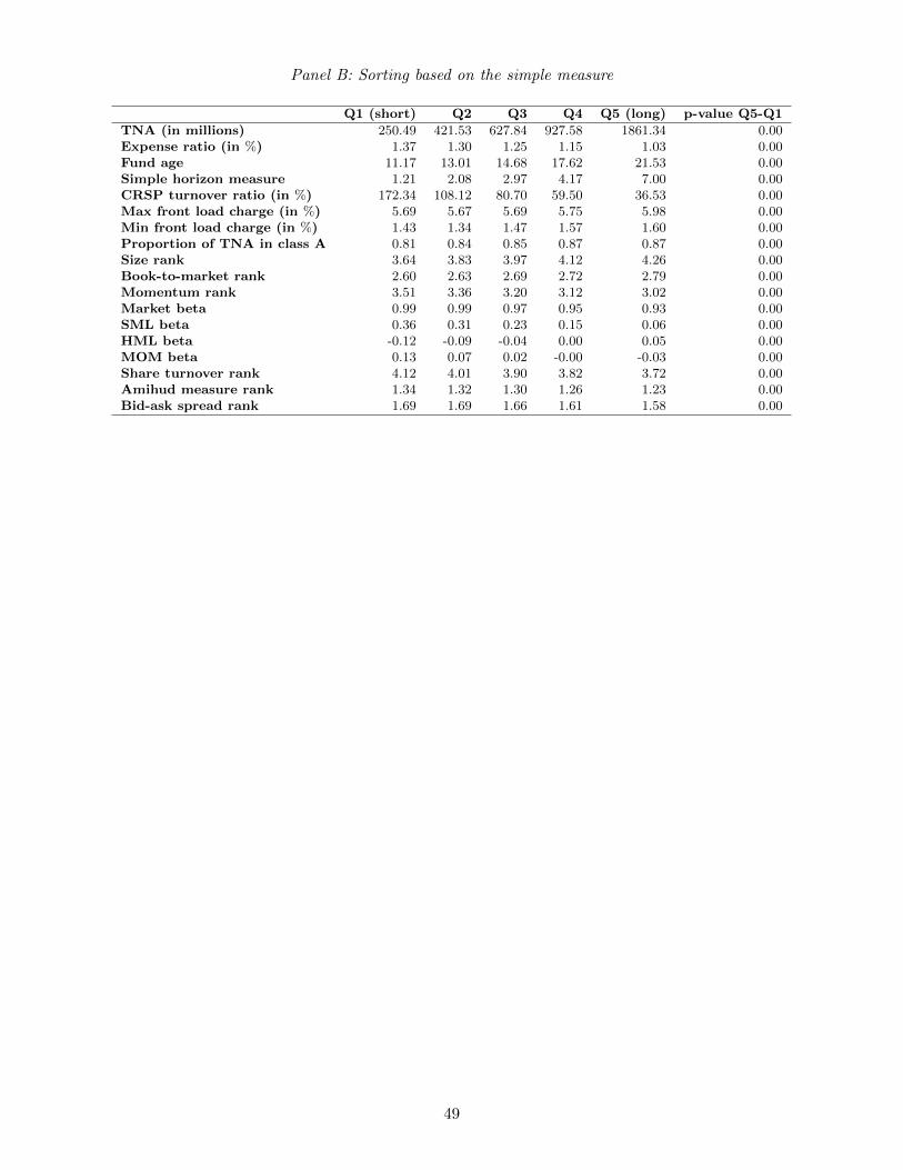
measures, then calculate the average fund and stock characteristics in each quintile. Panel B of Table 1
presents the results using the simple horizon measure.22 There are systematic differences between long
and short-term mutual funds in their characteristics and in their investment preferences. Notice that
total net assets and fund age increase with fund holding horizons and that expense ratio decreases with
fund holding horizons. Put differently, long-term funds are large and long-established funds with a rel-
21The share turnover is defined as the prior quarter average of the daily turnover ratio. The daily turnover ratio isdefined as the daily trading volume divided by the number of shares outstanding. We adjusted the volume of stocks tradedin the Nasdaq following Anderson and Dyl (2005).
22Results with the other horizon measures are qualitatively similar.
17
atively small expense ratio.23 Moreover, there is a wide dispersion in the fund investment horizons. For
example, the average simple measure in each fund quintile suggests that short-, medium-, and long-term
funds hold stocks for about one, three, and seven years, respectively. There are also clear patterns in
the characteristics of stock holdings of funds with different holding horizons. Long-term funds tend to
prefer larger companies, more value firms (high book-to-market), less past winners, and less popular but
at the same time more liquid stocks than short-term funds. These stock preferences are also reflected
in the factor exposures. Indeed, long-term funds exhibit lower market beta and exposure to the SML
factor than short-term funds. Furthermore, long-term funds have a positive (negative) exposure to the
HML (momentum) factor, whereas the sign of the exposure is reversed for short-term funds.
Since the 1990s, many funds offer multiple share classes representing ownership interests in the same
portfolio, but using different fee structures. The three share classes commonly offered by multiple-class
funds are denoted A, B and C.24 By offering different share classes mutual funds can try to cater to
different types of investors. Nanda et al. (2009) suggest that “investors with relatively long investment
horizons will prefer the A class with its up-front load and lower annual charges, while those with short
and uncertain horizons will prefer the B or C class.” An interesting question is whether long-term
mutual funds try to attract more long-term investors than short-term funds. This is important because
if this is not the case, then there could be some trade pressure to the manager due to short-term
investment decisions of mutual fund investors. Consistent with long-term funds catering to long-term
investors, Table 1 Panel B shows that long-term funds have more assets in share class A and charge
higher maximum and minimum front-end load fees than short-term funds.25
To better characterize how long a fund takes to accumulate or lower a position in a row, we calculate
the time span of consecutive purchases (sales) by a fund as the value-weighted average of time span of
23Despite the lower expense ratio, the revenue fees of long-term funds is not necessarily lower than short-term fundsgiven the difference in size.
24The A class is characterized by high front-end loads and low annual 12b-1 fees. The B and C classes typically have nofront-end loads but may charge a contingent deferred sales load upon exit and usually charge higher annual 12b-1 fees.
25Class A is identified in the sample as the share class that charges a front-end load. The maximum and minimum loadfees are computed among funds that charge a front-end load.
18
purchases (sales) of all stocks in the fund portfolio. The time span of a consecutive purchase must start
with the purchase of a stock and end with another purchase, with no sales in between. Similarly, the
time span of a consecutive sale must start with the sale of a stock and end with another sale, with no
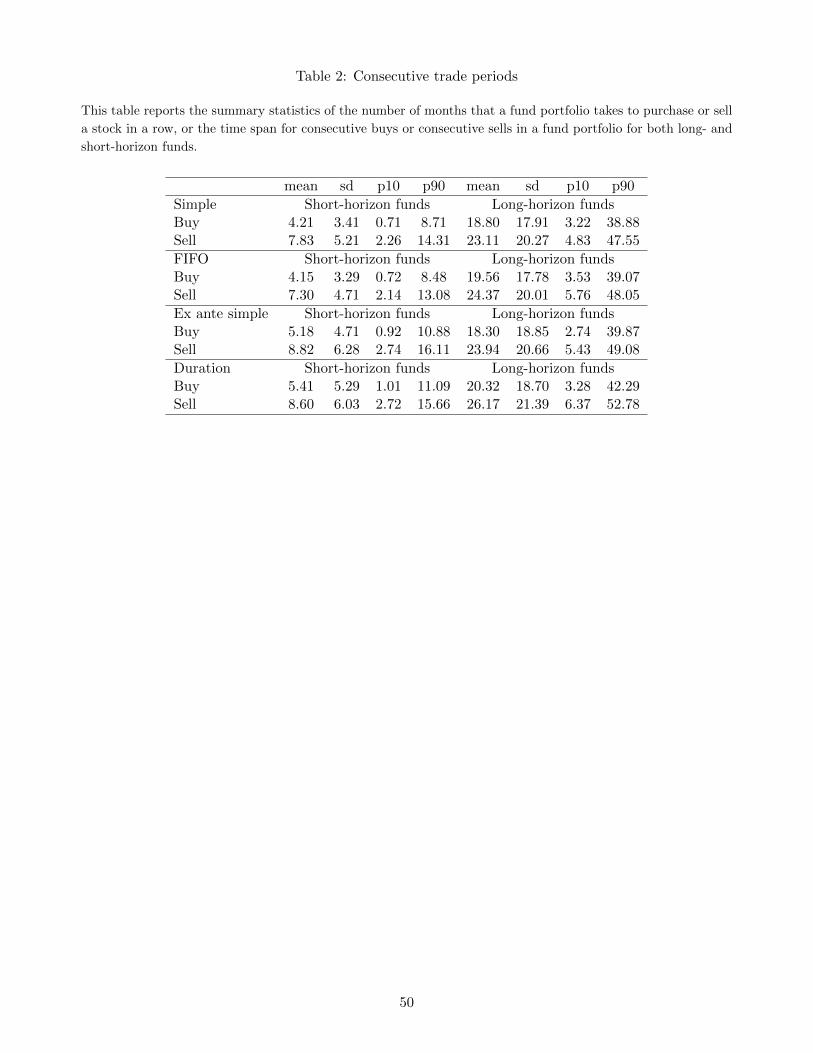
purchases in between. Table 2 reports the summary statistics of time span, in terms of the number of
months, that long-horizon and short-horizon funds use to purchase or sell a stock in a row.
Long-horizon funds take much longer time to either continuously increase or continuously decrease
their positions than short-horizon funds. Indeed, long-horizon funds take at least 18 (23) months on
average to accumulate (reduce) a position compared to four (eight) months for the short-horizon funds.
Interestingly and surprisingly, some long-horizon funds can take about three to four years to keep
increasing or decreasing a position. This finding suggests that long-horizon funds are able to take time
to strategically accumulate or curtail a position.
Table 3 reports the correlation matrix of our investment horizon measures, CRSP reported turnover,
and holdings-based turnover. While there is a high correlation among our measures of investment
horizons with values ranging from 0.77 to 0.89, the correlations between our horizon measures and
turnovers, especially CRSP reported turnover, are smaller in magnitude, around 0.5 in absolute value.
The correlations among long-horizon fund holdings that are constructed using different fund horizon
measures are quite high, roughly 0.7—0.9. The correlations among short-horizon fund holdings have a
similar magnitude. However, the correlation of LFH and SFH is quite low. This means that long- and
short-horizon funds are interested in different stock groups in general.
3.2 Persistence of fund horizon measures
If fund managers are skillful at exploiting private information that is profitable over different hori-
zons, we would expect that managers intentionally choose long-horizon investments or short-horizon
investments accordingly. An interesting question is whether horizon skills tend to persist. To check this
persistence, each month, we sort fund portfolios into quintiles according to one of our horizon measures,
19
the Simple, FIFO, Ex-Ante Simple, or Duration Measure. Q1 consists of funds with the lowest holding
periods and Q5 consists of funds with the highest holding periods. Figure 1 depicts the average fund
holding horizons of each quintile at the formation period and subsequent first to 20th quarter.
Fund investment horizons exhibit long-term stability. The ranking of the quintile portfolios in the
20th quarter after the formation period remains identical to that in the formation period. Take the
Simple Horizon Measure as an example. The average investment periods are 1.2, 2.2, 3.1, 4.3, and 6.9
years for the five quintiles at the formation period, while the average investment periods become 2.2,
2.7, 3.5, 4.3, and 6.6 years in the 20th quarter after the formation period. Moreover, this remarkably
persistent pattern is evident for both ex-post and ex-ante horizon measures. Thus, funds appear to
self-select into a particular type of holding horizon–long or short.
4 Empirical results on stock performance
In this section, we examine whether the consensus opinion of long-horizon funds contains information
about long-term stock performance, and whether the consensus opinion of short-horizon funds contains
information about short-term stock performance. The low and positive correlations between LFH
and SFH, as shown in Table 3, suggest that long- and short-horizon fund managers are generally
interested in different groups of stocks, although they may select some stocks in common. Moreover,
as mentioned earlier, both long- and short-horizon funds may select stocks for non-performance related
reasons. Therefore, we use relative holdings information of LFH minus SFH to classify stocks that
favored by one fund group vs. the other. This simple method can help to identify stock selection skills
due to differential information as opposed to other reasons for holding stocks. Similarly, we use the
relative trade information embedded in LFTrade minus SFTrade to single out stock groups that are
likely to reflect skills of long- relative to short-horizon fund managers. Then, we compare future stock
performance over different holding periods of stock portfolios that are preferred by long-horizon versus
20
short-horizon mutual funds.
4.1 Informativeness of fund holdings
We first examine whether fund holdings can provide valuable information about future stock perfor-
mance. Each month, stocks are grouped into quintiles according to the relative holdings of LFH minus
SFH. The top quintile (Q5) contains stocks that are held more by long- and less by short-horizon funds,
whereas the bottom quintile (Q1) consists of stocks that are held more by short- and less by long-horizon
funds. We then calculate buy-and-hold portfolio returns for each quintile portfolio over the next month
and up to the next five years after portfolio formation. Stocks in each quintile are weighted equally
at the formation month, then weights are updated following a buy-and-hold strategy. If a stock drops
out during a buy-and-hold period, we adjust the weights of the existing stocks. These buy-and-hold
portfolio returns are then averaged over time. Figure 2 shows the buy-and-hold portfolio performance
of the top and bottom quintiles over various holding periods, using either the Simple or ex-ante Simple
measure as the horizon measure. It also displays the return spread of the long-short position, which is
long the top quintile and short the bottom quintile, along with 10% confidence intervals.
The results indicate that stocks largely held by long-horizon funds exhibit much better long-term
performance than those largely held by short-horizon funds, whereas there is no evidence that stocks
largely held by short-horizon funds perform better in the short run. The first column of Figure 2 shows
that the buy-and-hold returns for stocks in the top quintile (Q5) are larger than those in the bottom
quintile (Q1) for all holding periods. Although those returns for both stock quintiles increase with the
holding period, the increase is much larger for the top quintile than for the bottom quintile. This leads
to an increasing positive spread of the long-short position. Consider the 5-year (20-quarter) performance
as an example. Using both measures, the top quintile exhibits an average buy-and-hold return of about
92%, whereas the bottom quintile exhibits an average buy-and-hold return of about 70%. The difference
is more than 22% for five years, or 4.4% per year, which is statistically and economically significant.
21
Even after adjusting for risk exposure using Carhart (1997) four-factor alphas or DGTW (1997)
adjusted returns, the long-term outperformance of stocks with large ownership by long-horizon funds is
still pronounced and there is no evidence of stock-picking abilities of short-horizon funds based on fund
holdings. Indeed, the last two columns of Figure 2 illustrate that both of the two risk-adjusted returns
for the top quintile increase with the holding horizon, whereas for the bottom quintile, the four-factor
alpha is negative and decreasing with the horizon, and DGTW-adjusted returns are close to zero at all
horizons. As a result, the abnormal returns for the long-short portfolio are significantly positive at all
horizons, and exhibit an increasing pattern with the holding horizon.26
Take the five-year horizon as an example. The four-factor alphas and DGTW adjusted returns for
the top quintile portfolio are about 4% and 14%, respectively, for both the Simple and ex-ante Simple
measures. For the bottom quintile portfolio, DGTW adjusted returns are roughly zero, and the four-
factor alpha are about −12% and −4% for the Simple and ex-ante Simple measures, respectively. As
a result, the abnormal returns on the long-short portfolio are at least about 8% and 13% in terms of
four-factor alphas and DGTW adjusted returns, respectively, over five years, or at least about 1.6% to
3.6% per year, both economically and statistically significant.
Overall, using both ex-ante and ex-post horizon measures, stocks with large ownership by long-
horizon funds have superior long-term performance, although the results using the ex-ante measure
are slightly weaker. Unreported results show that this finding is confirmed when we use the FIFO or
the Duration measure. Therefore, the informativeness of long-horizon fund holdings about superior
long-term stock performance is not driven by the use of future information in the construction of fund
investment horizon measures.27
The preceding results using fund holdings information along with the low correlation between LFH
26As a robustness check, we also use a five-factor model that includes the Carhart four factors plus Pastor and Stam-baugh’s (2003) liquidity factor. All results in this paper remain quite similar using the 5-factor alpha instead of the 4-factoralpha to measure abnormal returns.
27For instance, with ex-post measures of holding horizon, long-horizon investors may simply be those investors who werethe beneficiaries of more good luck, which motivated them to continue holding positions for a longer period.
22
and SFH imply that long- and short-horizon funds are generally interested in different groups of stocks.
One possibility is that stocks with superior long-term performance are different from stocks with good
short-term performance. Long-horizon fund managers target at and are able to select stocks with good
long-term returns. Another possibility is that a skilled long-term fund manager strategically avoids
picking a stock that is popular among short-horizon funds. Because short-term funds are likely to move
money in and out of a stock frequently, this behavior can generate a temporarily adverse price impact.
By not selecting such a stock, long-term funds avoid the adverse consequences of a temporarily adverse
price impact, such as experiencing fund outflows that follow underperformance in the short-run.
4.2 Informativeness of fund trades
Fund holdings and trades are likely to reflect managerial stock-picking talents differently for long- and
short-horizon funds. If fund managers are skillful in stock selection, fund holdings tend to incorporate
their current as well as historical superior information about the value of stocks, whereas fund trades
essentially reflect their current superior information. We therefore would expect that fund holdings
are more informative about long-horizon funds’ stock selection skills than trades. The rationale is that
if long-horizon funds apply techniques to select stocks with superior expected long-term performance,
they are likely to buy and hold those best picks for a long time. Those best picks appear in trades only
at the time of purchase (possibly a sequence of purchase), while they appear in fund holdings for a long
period. Moreover, long-horizon funds tend to hold but not frequently trade their best selected stocks.
On the other hand, they are likely to trade other stocks in their portfolio that are less attractive for
non-performance related reasons, such as to incorporate fund flows or to stay close to their benchmark.
In contrast, if short-horizon funds use techniques to select stocks with temporarily good returns, then
they have to trade quickly, otherwise, short-term profits can disappear. Therefore, fund trades can
be more useful than fund holdings to capture skills of short-term funds that are more likely to take
advantage of short-term information (see Chen et al., 2000). Accordingly, this section uses fund trades
23
to analyze stock selection skills.
Our first test investigates whether fund purchases reflect stock selection skills. We sort stocks
into quintiles based on long-horizon fund purchases relative to short-horizon fund purchases and then
study future performance of quintile portfolios. Specifically, stocks are assigned to five groups each
month based on positive LFTrade minus positive SFTrade. The top quintile includes stocks that are
purchased more by long-horizon funds than by short-horizon funds, and the bottom quintile consists
of stocks that are purchased more by short-horizon funds than by long-horizon funds. Since common
purchases from both long- and short-horizon funds can be driven by reasons others than selection skills,
our sorting based on the relative purchase can help to remove common non-skill related purchases, and
thus sharpens the identification of purchases related to differential selection skills.
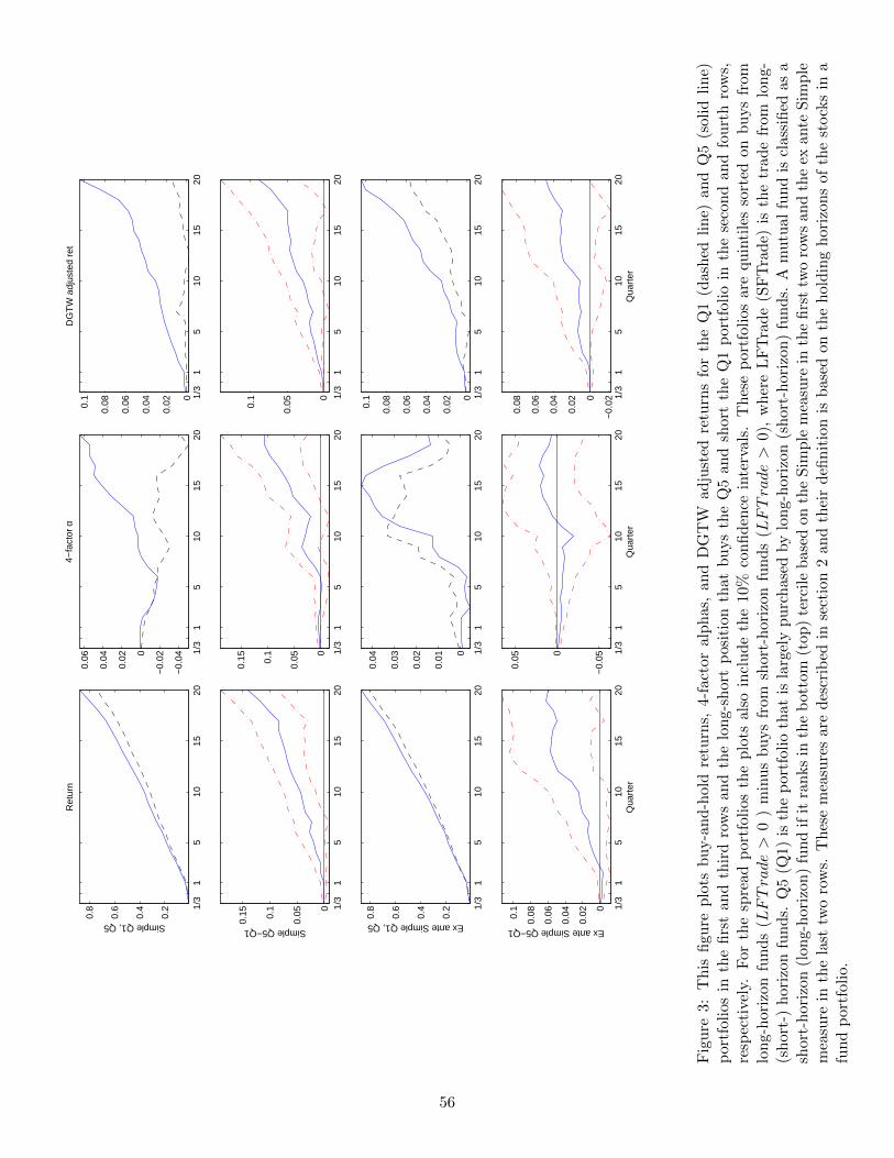
Figure 3 presents the stock portfolio performance for the top (Q5) and bottom (Q1) quintiles,
as well as for the long-short portfolio that buys the top quintile and sells the bottom quintile, over
next month and up to five years after the sorting month using the Simple and ex-ante Simple horizon
measures. A few points are noteworthy. First, different from the pattern based on fund holdings in
Figure 2, short-term performance of the bottom quintile can sometimes be better than that of the
top quintile. Second, we see some evidence that fund purchases can indicate skillful stock selection of
short-term funds. Stocks largely purchased by short-horizon funds can exhibit positive, although small,
abnormal returns. This is different from the result based on fund holdings in Section 4.1 where stocks
predominantly held by short-horizon funds have negative abnormal returns. Third, abnormal returns of
stocks that are largely purchased by long-term funds (Q5) are positive over the long term. Even so, they
are smaller in magnitude and less statistically significant compared with long-term abnormal returns
on stocks that are predominantly held by long-term funds, which are shown in Section 4.1. Finally,
the long-short portfolio that buys the top quintile and sells the bottom quintile has positive alphas and
positive DGTW adjusted returns at a long horizon. This result is also weaker than what obtained using
24
fund holding information. Overall, as expected, fund purchases reveal managerial skills of long-term
funds, but less effectively than fund holdings; fund purchases can weakly indicate managerial skills of
short-term funds.
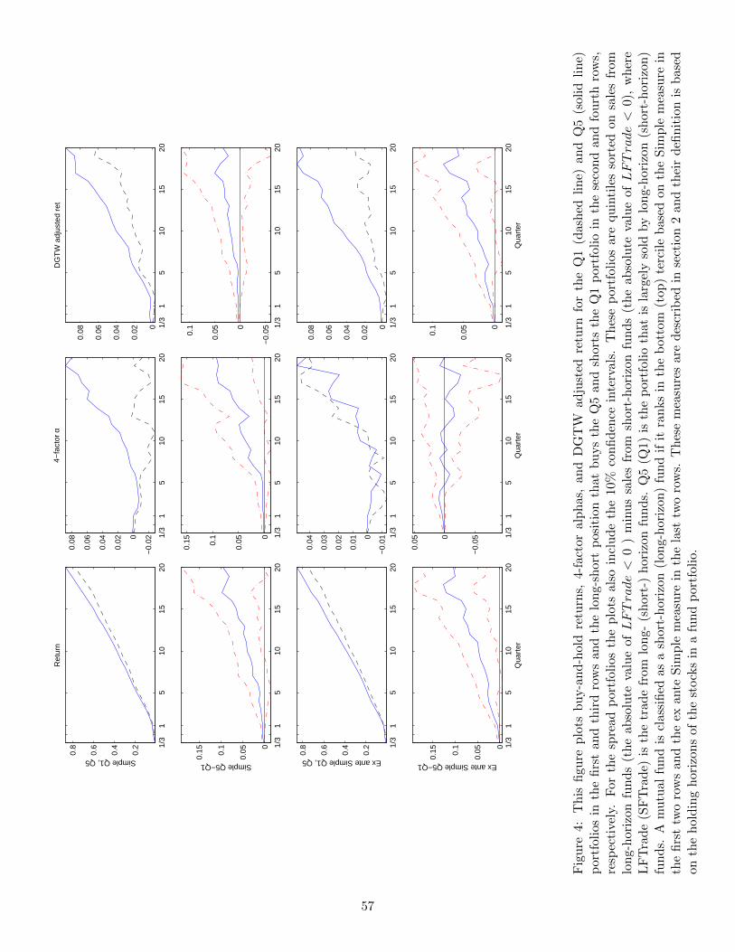
Similarly, we investigate the informativeness of fund sales. Stocks are sorted into quintiles based
on the relative sales by long-horizon funds versus sales by short-horizon funds, or the absolute value of
negative values of LFTrade minus the absolute value of negative values of SFTrade. The top quintile
(Q5) includes stocks that are sold largely by long-horizon funds relative to short-horizon funds, while
the bottom quintile (Q1) consists of stocks that are sold predominately by short-horizon funds. Figure
4 presents results using the Simple and ex-ante Simple horizon measures.
Notice that stocks in Q5 that are sold largely by long-horizon funds generally exhibit good abnormal
returns at a long horizon. One possible explanation is that long-horizon funds are able to pick stocks
with good long-run returns. Even though they sell some of their holdings due to outflows or to exploit
new investment opportunities, these stocks continue to perform well after they sell. Another possible
explanation is that long-horizon funds sell some stocks early because they want to realize some profits
and reduce the risk of holding the position. In addition, we notice that short-term fund sales indicate
short-term poor performance. Stocks largely sold by short-horizon funds tend to have negative abnormal
returns.
4.3 Long holding-period stocks versus short holding-period stocks
If long-horizon fund managers are skillful in selecting stocks with good long-run performance, we
would expect that stocks that are actually held by long-horizon funds for a long period perform better
than stocks that these same funds hold for a short period. Similarly, if short-horizon fund managers
are skillful at selecting stocks with good short-run performance, we would expect that stocks that are
actually held by short-horizon funds for a short period perform well in the short term. This section refines
the informativeness of fund holdings and fund trades about selection skills by distinguishing stocks that
25
are on average held for a long or short period in long-horizon or short-horizon fund portfolios.
We first define average holding horizons of stocks. Let hi,j,t denote the holding horizon of stock
i held in fund j at time t, then the average holding horizon of stock i owned by long-horizon funds,
long-horizon fund holding period, is defined as
hslongi,t =
M longi,t∑j=1
ηi,j,thi,j,t, (6)
where M longi,t is the number of long-horizon funds that hold stock i at time t, and ηi,j,t is the ratio of
number of shares of stock i held by fund j divided by the total number of shares of stock i held by all
long-horizon funds at time t. Similarly, we define the short-horizon fund holding period of stock i as
hsshorti,t =
Mshorti,t∑j=1
ηi,j,thi,j,t. (7)
If the long-horizon fund holding period of a stock is larger (smaller) than the median holding period
among all stocks that are owned by long-horizon funds, then we say this stock has a long (short) holding
period by long-horizon funds. Analogously, if the short-horizon fund holding period of a stock is larger
(smaller) than the median holding period among all stocks that belong to short-horizon funds, then we
say this stock has a long (short) holding period by short-horizon funds.
We consider four stock portfolios that are constructed as follows. First, we classify stocks into
quintiles each month based on LFH minus SFH, with Q5 consisting of stocks that are largely held
by long-horizon funds, and Q1 consisting of stocks that are largely held by short-horizon funds, as we
have done in section 4.1. Then we divide stocks in Q1 (Q5) into two groups depending on whether
the short-horizon (long-horizon) fund holding period of a stock is above the median holding period for
all stocks belonging to short-horizon (long-horizon) funds. Using the ex ante Simple measure, Figure 5
presents the performance, along with the 10% confidence intervals, for the four stock portfolios in the
next month, and up to the next five years after the portfolio formation month.
Clearly, stocks that have a long holding period by long-horizon funds have the best long-term future
26
performance among the four stock groups. For example, at a five-year horizon, this group of stocks
obtain the buy-and-hold return of 94%, the four-factor alpha of 7%, and the DGTW adjusted return of
14%, the highest values among four groups. All these gross and abnormal returns are all statistically
and economically significant. In contrast, there is mixed evidence of good long-term performance for
stocks that have a short holding period by long-horizon funds; and there is no evidence of short-term
good performance for stocks that have a short holding period by short-horizon funds. Overall, these
results suggest that the long-run outperformance of long-horizon funds stems from their long-term stock
positions.
Similarly, we combine fund purchase information and stock holding periods to form four stock
portfolios and examine the future performance of these four portfolios. In unreported results, we notice
that stocks that are largely purchased by long-horizon funds and are held for a long period have the
best long-term performance among the four stock groups. In addition, there is weak evidence of good
short-term performance of stocks that are largely purchased by short-horizon funds and are held for
either a short or a long period. These results further confirm that fund trades contain information
regarding the selection skills of both long-horizon and short-horizon funds.
4.4 Cash-flow information
In this section, we delve into a central issue regarding the economic source of managerial skills:
the fundamental cash-flow information reflected in funds’ stock selection. If fund managers take use of
information related to firm fundamentals in picking stocks, then we would expect that long-horizon fund
managers are skillful at exploiting long-term firm fundamentals, and that short-horizon fund managers
are good at using short-horizon fundamental information. Therefore, we would expect the pattern of
future cash-flow information for different stock portfolios to be analogous to the pattern of future stock
portfolio returns that have been discussed in previous sections.
To measure information shocks to firm fundamentals, we use four variables: cash-flow news (CFnews),
27
analyst forecast revisions (FRV ), earnings-announcement-window returns (EAR), and risk-adjusted
EAR.28 CFnews is the cash-flow component of unexpected quarterly returns and is obtained via a
Campbell-Shiller decomposition. The Appendix describes the details of the construction of this vari-
able. FRV is the consensus EPS forecast for the current fiscal year, minus the three-month lagged
consensus EPS forecast for the same fiscal year, divided by the stock price three months ago. EAR
is the buy-and-hold return during the [-1, +1] trading-day-window around an earnings announcement
date.29 If earnings are announced during a non-trading day, we treat the next immediate trading day
as the announcement date. Adjusted EAR is the EAR minus the buy-and-hold return of the NYSE,
AMEX, and Nasdaq market index during the same trading-day-window. To reduce the effect of out-
liers, all these information variables are cross-sectionally winsorized at the top and bottom 1%. These
four variables capture fundamental shocks from different perspectives: CFnews captures revisions of
expected future cash flows over an infinite horizon that are reflected in stock returns. FRV reflects
changes in earnings expectations for the current fiscal year, presumably due to new information arrival
during the quarter. EAR and adjusted EAR measure the magnitude of investors’ earnings surprises in
terms of stock returns and stock abnormal returns, respectively.
Figure 6 displays cumulative cash-flow information over the next 1 to 20 quarters following the
stock portfolio formation date. Specifically, we first sort stocks into quintiles according to relative fund
holdings or trades, as we did in the previous sections. Then we calculate the cross-sectional mean of
each information variable in the nth quarter after the formation quarter, where 1 ≤ n ≤ 20, and we
proceed to cumulate these quarterly means over one to 20 quarters. Finally, we compute an average
across all portfolio formation dates for each of these cumulated measures.
Let us first focus on the first two rows for the cash-flow results using fund holdings to sort stocks.
28Since EAR is available only at the quarterly frequency, we construct all variables of information shocks at the quarterlyfrequency for simplicity.
29We also use EAR as buy-and-hold return during the [-2, +2] trading-day-window around an earnings announcementdate. Both definitions of the EAR deliver very similar results in our tests to follow.
28
Notice that all four cumulative fundamental variables are positive, and increase with holding horizons
for stocks that are largely held by long-horizon funds (Q5). Untabulated results confirm that these
positive cumulative cash-flow results for Q5 are statistically significant. This result suggests that the
long-run outperformance of stocks predominantly held by long-horizon funds is associated with superior
long-term firm fundamentals. In contrast, cumulative cash-flow variables can be negative (CFnews),
positive (FRV ), or close to zero (EAR and adjusted EAR) for stocks that are largely held by short-
horizon funds (Q1). All of these four cash-flow variables for the long-short portfolio that buys Q5 and
sells Q1 are significantly positive at the horizons of six quarters and longer.
When relative fund purchase is used to group stocks, as shown in the third and fourth rows of Figure
6, stocks largely purchased by short-horizon funds (Q1) have stronger short-term cash flows than stocks
largely purchased by long-horizon funds (Q5). All four variables at a short horizon for the long-short
portfolio that buys Q5 and sells Q1 are negative, and two of them, CFnews and FRV , are statistically
significant. On the other hand, long-term firm fundamentals are stronger for stocks predominantly
purchased by long-horizon funds (Q5) relative to those largely purchased by short-horizon funds (Q1).
In the long run, all four fundamental variables for the long-short portfolio are positive. CFnews is
statistically significant at horizons of one year and longer. When relative fund sale is used to group
stocks, we see that, in the last two rows of Figure 6, cumulative cash flows at a long horizon are stronger
for stocks largely sold by long-horizon funds (Q5) than those largely sold by short-horizon funds (Q1).
This result again indicates that firm fundamentals remain attractive after stocks are sold by long-horizon
funds.
We also check future cash flows of stock portfolios in terms of the cash-flow component of buy-
and-hold portfolio returns instead of cumulative cash-flow variables. Specifically, using a buy-and-hold
portfolio approach, we replace returns with the cash-flow variables, keeping the same portfolio weights
as we calculate buy-and-hold portfolio returns. This calculation can be roughly regarded as the cash-
29
flow component of a buy-and-hold portfolio return. The message is very similar to what we get using
cumulative cash-flow variables.
In summary, the patterns of portfolio performance in terms of cash flows are quite analogous to
the pattern in terms of portfolio returns. These cash-flow results indicate that stock selection skills are
associated with superior ability in exploiting firm fundamentals. Long-horizon fund managers are able
to buy and hold stocks with strong long-term firm fundamentals, and that short-horizon fund managers
can buy stocks with temporarily good cash flows.
5 Empirical results on fund performance
In this section, we examine the relation between fund investment horizon and performance at the
mutual fund level, using both a sorted fund portfolio approach and Fama-MacBeth regressions that
control for fund characteristics.
5.1 Fund performance using a sorted portfolio approach
First, using a sorted fund portfolio approach, we group funds into quintiles each month based on the
different fund horizon measures that we have discussed in Section 2.1. For each quintile, we calculate
the buy-and-hold cumulative fund portfolio returns at a horizon of the next month, and up to the next
five years.30 Portfolio weights are equal at the formation month, then updated following a buy-and-hold
strategy. Finally, we average these buy-and-hold returns over time for each quintile and for each holding
horizon. To proxy fund returns, we use both CRSP reported fund net returns after expenses, and fund
total returns that are fund net returns plus 112 times the most-recent fund expense ratio. Fund net
returns are compensation that fund investors can actually obtain, whereas fund total returns can be
taken as the sum of compensation to both fund investors and fund managers, net of portfolio trading
30Most of the existing mutual fund literature focuses on short-term performance considering a window of no greater thanone year to measure future abnormal returns. One exception is Frazzini and Lamont (2008) who focus on future long-runstock performance.
30
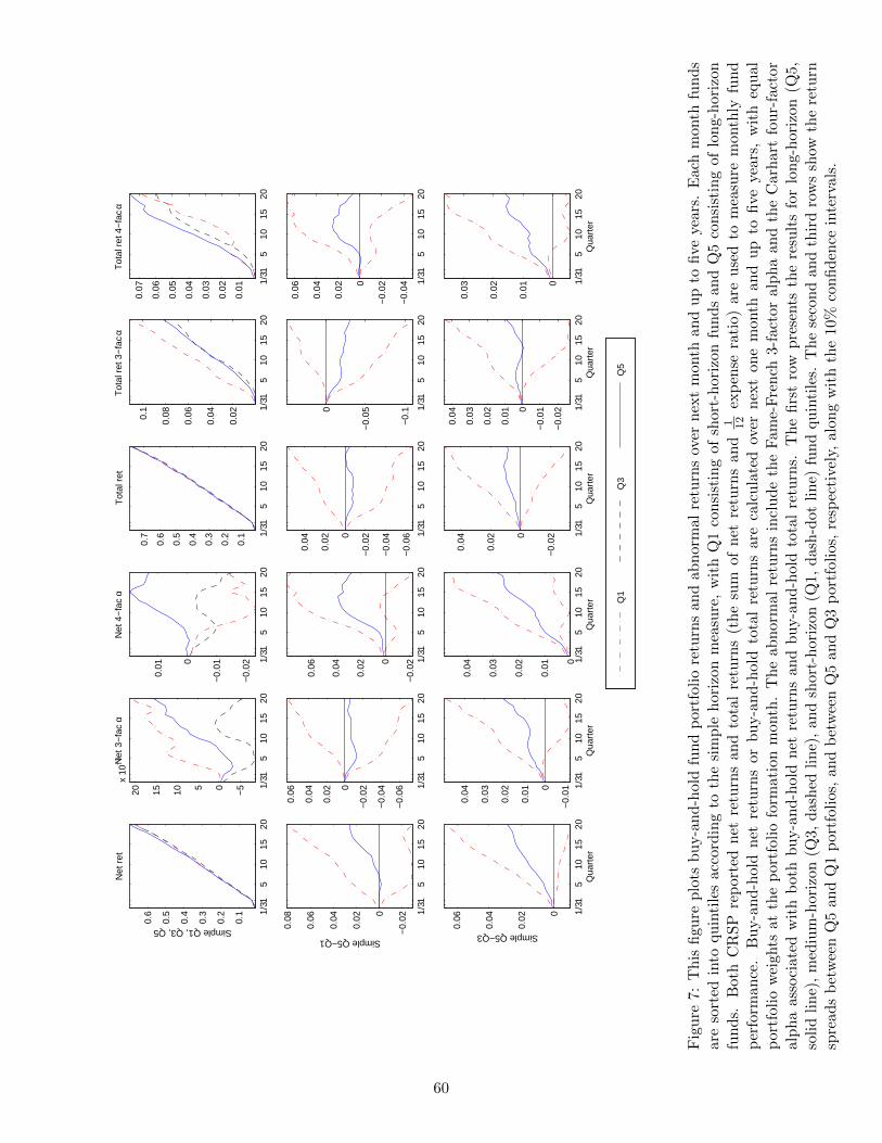
costs. Table 4 summarizes the portfolio performance in fund quintiles that are sorted on the Simple
horizon measure at a horizon of one month, one quarter, and one to five years, and Figure 7 displays the
result over horizons ranging from one month to five years for the first, third, and fifth fund quintiles.
Two points are noteworthy for the results using fund net returns in the first three columns of Table
4. First, there is a clear U-shaped fund performance in terms of both buy-and-hold net returns and
3-factor alphas with respect to fund holding horizons. In terms of buy-and-hold net returns, the best
performers are long-horizon funds in general, and short-horizon funds rank second. These orders are
reversed in terms of 3-factor alphas. Take the three-year horizon as an example. The buy-and-hold net
return is 37.8% for short-term funds in Q1, decreasing to 36% in Q2, and then increasing to the best
performance of 38.5% for long-horizon funds in Q5. The 3-factor alpha decreases from 1.5% in Q1 to
almost zero in Q3 and then increases to 0.8% in Q5. Interestingly, once we control for momentum with
the 4-factor model, the U-shaped pattern disappears at some holding horizons, for example, the three-
year horizon, and long-horizon funds become the best performers. Moreover, the 4-factor alphas for
short-horizon funds are much lower than the 3-factor alphas. Take the three-year horizon as an example
again. The 4-factor alphas are −2.3%, −0.3%, 1.4% for the short-, medium-, long-horizon funds in
Q1, Q3, Q5, respectively. These results suggest that short-horizon funds generate alphas largely from
momentum strategies. Once the momentum factor is controlled for, the performance of short-horizon
funds becomes poor. These results are also consistent with the summary statistics shown in Table 1,
that short-horizon funds prefer past winners.
Second, long-horizon funds outperform short- and medium-horizon funds in the long term, whereas
short-horizon funds perform no better than long-horizon funds in the short term, according to the 4-
factor alphas. Take the three-year holding horizon as an example. The long-short portfolio that buys
long-horizon funds in Q5 and sells short-horizon funds in Q1 earns roughly 3.6% in terms of the 4-factor
alpha, or 1.2% per year, which is statistically and economically significant. On the other hand, the
31
4-factor alpha for this long-short portfolio is also positive for a short period, such as one month or one
quarter, so short-horizon funds do not perform better than long-horizon funds in the short term.
Table 4 also reports fund performance in terms of total returns, which add back expense ratios to
net returns. Compared with the results based on net returns, a few differences exist. First, there is also
a U-shaped relation between buy-and-hold total returns and fund holding horizons, but short-horizon
funds tend to perform the best. Moreover, the long-short portfolio that buys the long-horizon funds
in Q5 and sells either short-horizon funds in Q1 or medium-horizon funds in Q3 earns lower alphas,
compared with the result using net returns. The reason is that expense ratios decrease with fund holding
horizons, as shown in Table 1, so short-horizon fund performance increases more than long-horizon fund
performance after expense ratios are added back to total fund returns. Furthermore, long-horizon funds
earn a significantly positive 4-factor alpha using total returns, where they earn insignificant and a
much small 4-factor alpha using net returns. This result means that long-horizon fund managers have
stock picking-skills, but fund managers and fund expenses consume almost all of the value of active
management. Finally, short-horizon funds earn an insignificantly positive 4-factor alpha in the short
run using total returns, whereas they earn a negative or even significantly negative 4-factor alpha using
net returns. This finding suggests that short-horizon funds, on average, do not have enough skill to cover
their fees and expenses, and, therefore, might make fund investors worse off, compared to a low-cost
index fund.
We also investigate the relation between fund investment horizons and fund performance using the
ex ante horizon measures. The results are similar to, but weaker than the results using the Simple
measure. One possible reason is that the ex-ante measures, by construction, assign a short holding
horizon when a stock position is newly initiated, even if this stock is held for a long period. This can
weaken the ability of the ex-ante measures to capture fund investment horizons.
Comparing these results in the fund-level analysis with the results in the stock-level analysis, we see
32
that the latter are more supportive than the former of the notion that long-horizon funds are capable
of picking stocks with good long-run performance and short-horizon funds are skillful in identifying
stocks with good short-run performance. The reason is that fund portfolios include stocks that are
held for a variety of non-performance reasons, such as benchmark tracking; whereas our constructed
stock portfolios reflect differential aggregate consensus opinions of long-horizon funds over short-horizon
funds, and this approach partially removes non-skill related common stock-picking and sharpens the
results. Therefore, the stock-level analysis is more effective in revealing manager selection skills.31
5.2 Fund performance using Fama-MacBeth regressions
Prior studies have documented that fund characteristics play an important role in determining fund
performance and portfolio choice. Therefore, in further tests, we control for fund characteristics in the
examination of the relation between fund performance and fund holding horizon. Specifically, in each
month we run cross-sectional regressions of abnormal buy-and-hold fund returns on one of our horizon
measures, controlling for a list of fund characteristics including fund age, log fund TNA, fund expense
ratio, growth fund dummy, past year fund flow, as well as flow volatility and fund return volatility over
the past year.32 We calculate means of the time series of coefficient estimates, following the Fama-
MacBeth (1973) approach. Since our dependent variables overlap on a monthly frequency, standard
errors are calculated using the Newey and West (1987) approach to account for autocorrelation and
heteroskedasticity. We use as dependent variable the 4-factor alphas obtained using either fund net
returns or fund total returns.
Figure 8 reports coefficient estimates over horizons ranging from one month to five years using the
ex ante Simple measure, with the first two rows containing results using fund net returns, and the last
two rows using fund total returns. We see that fund abnormal returns increase almost linearly with
31For example, when we use the inverse of CRSP turnover to classify funds into long- or short-horizon funds, as we willdiscuss in Section 6, we see evidence of stock selection abilities of long-horizon funds using our stock portfolio approach,but little evidence using the fund portfolio approach.
32Growth funds are classified following the approach of Hunter et al. (2014).
33
fund holding horizons over horizons of more than one year, and that this positive relation is statistically
significant over horizons of more than two and half years. Take the five-year coefficient as an example. A
one standard deviation increase in fund holding horizon increases fund abnormal performance by about
2.8% over a five-year horizon. The result is stronger if ex-post horizon measures are used. Interestingly,
fund age significantly and negatively affects fund performance. This is consistent with Pastor et al.
(2014), who find that performance deteriorates over a typical fund’s lifetime.33 Because fund age
increases with fund holding horizons, as shown in Panel B of Table 1, our fund sorting portfolio approach
cannot disentangle these two offsetting effects, leading to a weak relation between fund performance
and fund investment horizons. Moreover, fund expense ratios significantly decrease fund net returns.
Consistent with the literature, growth funds have superior short-run performance but little long-run
advantage.
6 Using the inverse of turnover as a fund horizon measure
To compare our results with the literature, we use the (inverse) turnover ratio as an alternative
measure of fund investment horizon. If we assume that funds with a high level of trading activity
measured by the turnover ratio generally hold stocks for a short period, whereas funds with a low level
of trading activity generally hold stocks for a long time, then the inverse of turnover can be a proxy for
fund holding horizon. Indeed, a turnover ratio computed from 13-F holdings data has been used in the
institutional investor literature to classify investors as short or long-term. The mutual fund literature
provides mixed evidence on the relation between turnover ratio and fund performance. Wermers (2000)
show that high-turnover mutual funds have better stock selection skills than low-turnover funds (a
similar result is provided by Yan and Zhang, 2007, for institutional investors). By contrast, Carhart
(1997) documents a negative association between turnover ratio and net fund performance.
33Pastor et al. (2014) find evidence of industry-level, instead of fund-level, decreasing returns to scale, which couldexplain the above pattern. Consistent with their finding, our tests indicate no evidence of a fund-level economy of scale,as indicated by the insignificant coefficient on size (log TNA).
34
Following the same sorted fund portfolio approach as we did in Section 5.1, we examine the relation
between fund performance and investment horizon that is measured by the inverse of CRSP turnover
instead of the Simple measure. Because CRSP turnover is widely used in the mutual fund literature,
our discussion here focuses on the results using the inverse of CRSP turnover. Figure 9 shows the
results, different from those in Figure 7. A few points are noteworthy. First, funds with high turnover
(Q1) outperform their low-turnover peers (Q5). When fund gross returns are used, the four-factor
alpha associated with funds with high turnover (Q1) is significantly positive. Moreover, it significantly
higher than the four-factor alpha for funds with low turnover (Q5) at horizons of one year or less. The
difference is about 1% a year. These results indicate that managers of funds with higher levels of trading
activities have skills to pick stocks with good short-term performance. When fund net returns are used,
the four-factor alpha is not statistically distinguishable from zero. The spread of the four-factor alpha
for Q5-Q1 is negative, but insignificant for a short period. Furthermore, we see only weak evidence that
funds with low turnover (Q5) outperform funds with high turnover (Q1) in the long term. These results
indicate that despite of manager skills for funds with higher turnover, the value of skillful stock-picking
is either retained by fund managers or consumed by fund expenses, and fund investors do not benefit.
We further run Fama-MacBeth regressions of fund abnormal returns on the inverse of CRSP turnover
along with other fund characteristics, as we discussed in Section 5.2. Unlike our fund horizon measures,
the inverse of CRSP turnover does not play a significant role in forecasting future fund performance.
Therefore, our horizon measures are essential to capture stock-picking skills of managers with long
investment horizon.
Why do our holdings-based horizon measures better reveal skills of long-horizon fund managers,
while CRSP turnover better captures stock-picking skills of short-term fund managers? The reason is
that, although turnover better capture trading activities, our measures more richly capture fund holding
horizons, especially long horizons. Turnover tends to miss out positions that have been held for a long
35
period. Put differently, turnover cannot adequately reflect the right tail distribution of holding periods
of stocks held in a fund portfolio.34 Although levels of trading activities and fund holding horizons
are negatively correlated, the correlations are far from perfect. Table 3 shows that the correlations
between the CRSP turnover ratio and our horizon measures is as low as −0.43. On the other hand,
CRSP reported turnover, not holding-based turnover, reflects intraquarter trading, while our measures
do not. Puckett and Yan (2011) show that intraquarter trading earns positive abnormal returns, so the
measures constructed using low-frequency fund holdings have a downward bias in capturing short-term
selection skills because of their inability to account for interim trades.
7 Conclusions
Using newly proposed direct measures of fund investment horizon, this paper examines the relation
between fund investment horizons and manager skills and further explores the economic sources of
stock selection skills for managers with different investment horizons. We use two approaches, one
at the stock-level and the other at the fund-level, to examine the relation. The stock-level approach
aggregates consensus opinions of the value of a stock from long- and short-horizon funds separately and
investigates stock performance over various holding horizons. The fund-level approach directly examines
the relation between fund performance and fund holding horizons.
In the stock-level analysis, we find that the stock-holdings, in aggregate, of long-horizon funds provide
valuable information about the long-term superior abnormal returns of a stock, whereas aggregate short-
horizon fund holdings provide little information about the short-term abnormal returns of a stock.
Interestingly, aggregate fund trades are informative about the stock selection skills of both long-horizon
funds and short-horizon funds, and aggregate long-horizon fund trades are less informative than holdings.
We also delve into the economic sources of stock selection skills of fund managers with different
34A recent paper by Chakrabarty et al. (2014) further discusses some of the issues associated with using turnover rateas a proxy for investment horizon.
36
investment horizons, that is, the fundamental cashflow information that is reflected in funds’ stock-
holdings or trades. We find that shocks mostly held by long-horizon funds are associated with superior
long-term firm fundamentals, whereas stocks largely purchased by short-horizon funds have better
short-term cashflow news relative to the stocks largely purchased by long-horizon funds. This finding
indicates that long-horizon fund managers are skillful in analyzing long-term firm fundamentals, and
achieve good long-run performance, and that short-horizon fund managers make use of short-term
cashflow information to make small profits.
In this fund-level analysis, we use both a ranked fund portfolio approach and Fama-MacBeth regres-
sions that control for fund characteristics. Using the ranked fund portfolio approach, we find superior
buy-and-hold (pre-expense) gross return performance of long-horizon funds, but this superior perfor-
mance is not present for buy-and-hold net returns. Thus, fund management captures long-horizon
fund skill-based returns, while fund investors benefit little, consistent with Berk and Green (2004) and
Grossman and Stiglitz (1980). Fama and MacBeth regressions indicate that investment horizon is a sig-
nificant predictor, with a positive coefficient, of future fund abnormal net returns even after controlling
for several fund characteristics.
In conclusion, this paper is the first that shows superior long-run performance of stocks largely held
or purchased by long-horizon funds. We also proposed the investment horizon as a useful novel proxy for
investment skill. The finding of the superior performance of long-term funds critically depends on the
use of more direct measures of fund investment horizons than what was previously used in the mutual
fund literature. There is empirical evidence that individual investors have long rebalancing horizons.
Ameriks and Zeldes (2004) find that, for a sample of defined contribution retirement plan participants,
47% (21%) made no changes (one change) to their allocation of contributions over a ten-year period.
Similar results are found for 401(k) plans by Mitchell et al. (2006). Our fund-level analysis suggests
that individual investors with long rebalancing horizons are better off selecting long-horizon funds rather
37
than short-horizon funds.
38
Appendix
A.1 Construction of cash-flow news (CFnews)
This measure accounts for changing expectations of the sum of discounted firms’ future cash flows
over all future periods. It is constructed using Institutional Brokers Estimate System (IBES) summary
unadjusted file. Monthly analyst earnings forecasts allow us to measure cashflow news at the monthly
frequency. Specifically, we keep consensus earnings forecasts for the current and subsequent fiscal
year (FE1t , FE2t ), along with its long-term growth forecast (LTGt ). The earnings forecasts are
denominated in dollars per share, and the t subscript denotes when a forecast is employed. The long-
term growth forecast represents an annualized percentage growth rate and pertains to the next three to
five years.
Similar to Frankel and Lee (1998), Pastor, Sinha, and Swaminathan (2008), Da and Warachka
(2009), Da, Liu, and Schaumburg (2012), and Balduzzi and Lan (2013), we use a three-stage model to
construct cash flow news by taking advantage of multiple earnings forecasts for different maturities. Let
Xt,t+j denote the time-t expectations of future earnings at t + j. In the first stage, expected earnings
are computed directly using analyst forecasts as follows:
Xt,t+1 = FE1t, (A.1)
Xt,t+2 = FE2t, (A.2)
Xt,t+3 = FE2t(1 + LTGt), (A.3)
Xt,t+4 = Xt,t+3(1 + LTGt), (A.4)
Xt,t+5 = Xt,t+4(1 + LTGt). (A.5)
In the second stage, expected earnings are assumed to converge to an economy wide steady-state
growth rate gt from year six to year 10. Specifically,
Xt,t+j+1 = Xt,t+j [1 + LTGt +j − 4
5(gt − LTGt)], for j = 5, . . . , 9. (A.6)
39
The steady-state growth rate gt is the cross-sectional average of LTGt.
Following Da and Warachka (2009), Da, Liu, and Schaumburg (2012), and Balduzzi and Lan (2013),
we assume the cash flow payout is equal to a fixed portion (Ψ) of the ending-period book value. Under
this assumption, the clean surplus accounting identity implies that the evolution of expected book value
is Bt,t+j+1 = (Bt,t+j +Xt,t+j+1)(1−Ψ). The parameter Ψ is set to 5% since this percentage is close to
the average payout rate for the firms in our sample.
In the third stage, expected earnings growth converges to gt , which implies expected accounting
returns converge to gt1−Ψ beyond year 10. The expected log accounting returns et,t+j is estimated at
time t as:
et,t+1+j ={ log(1 +
Xt,t+1+j
Bt,t+j) for 0 ≤ j ≤ 9
log(1 + gt1−Ψ) for j ≥ 10
(A.7)
The three-stage growth model implies expected future cash flows:
Et
∞∑j=0
ρjet+1+j =9∑
j=0
ρjet,t+1+j +ρ10
1− ρlog(1 +
gt1−Ψ
), (A.8)
where ρ results from the log-linear approximation (Campbell and Shiller, 1988) and equals 0.96 in our
sample. After ten years, the annualized discount factor ρ = 0.96 means that the remaining cash flows
exert little influence on the cashflow news. Vuolteenaho (2002) shows that the cash flow news are the
difference between cash flow expectations over consecutive months:
CFnewst+1 = Et+1
∞∑j=0
ρjet+1+j − Et
∞∑j=0
ρjet+1+j (A.9)
where CFnewst denotes cashflow news at time t.
40
A.2 Construction of holding-based turnover
Each quarter we calculate aggregate purchase and sales for each fund:
buyj,t =
Mj,t∑i=1
Ni,j,t>Ni,j,t−1
|Ni,j,tPi,t −Ni,j,t−1Pi,t−1 −Ni,j,t−1∆Pi,t|
sellj,t =
Mj,t∑i=1
Ni,j,t<Ni,j,t−1
|Ni,j,tPi,t −Ni,j,t−1Pi,t−1 −Ni,j,t−1∆Pi,t|,
where Pi,t are share prices for stock i at the end of quarter t. Fund j’s turnover, or churn rate, for
quarter t is then calculated as:
CRj,t =min(buyj,t, sellj,t)∑Mj,t
i=1Ni,j,tPi,t+Ni,j,t−1Pi,t−1
2
(A.10)
Then, we average this quarterly churn rate over the past year or, alternatively, past three years, to get
holding-based turnover.
41
References
[1] Alexander, G., G. Cici, and S. Gibson, 2007, Does motivation matter when assessing trade perfor-
mance? An analysis of mutual funds, Review of Financial Studies 20, 125-150.
Ameriks, John, and Stephen P. Zeldes, 2004, How do household portfolio shares vary with age?
Working paper, Columbia University.
Amihud, Y., 2002, Illiquidity and Stock Returns: Cross-Section and Time-Series Effects, Journal
of Financial Markets, 5, 31–56.
Amihud, Y., and R. Goyenko, 2013, Mutual fund’s R2 as predictor of performance, Review of
Financial Studies 26, 667-694.
Baker, M., L. Litov, J. Wachter, and J. Wurgler, 2010, Can mutual fund managers pick stocks?
Evidence from their trades prior to earning announcements, Journal of Financial and Quantitative
Analysis 45, 1111-1131.
Balduzzi, P., and C. Lan, 2013, Survey Forecasts and the Time-varying Second Moments of Stock
and Bond Returns, working paper.
Berk, J., and R. Green, 2004, Mutual fund flows and performance in rational markets, Journal of
Political Economy 112, 1269–1295.
Brown, K., V. Harlow, and L. Starks, 1996, Of tournaments and temptations: An analysis of
managerial incentives in the mutual fund industry, Journal of Finance 51, 85-110.
Bushee, B. 2001, Do institutional investors prefer near-term earnings over long-run value? Con-
temporary Accounting Research 18, 207-246.
Cai, F., and L. Zheng, 2004, Institutional Trading and Stock Returns, Finance Research Letters 1,
178-189.
Carhart, M., 1997, On persistence in mutual fund performance, Journal of Finance 52, 57-82.
42
Campbell, J., and R. Shiller, 1988, The dividend-price ratio and expectations of future dividends
and discount factors, Review of Financial Studies 1, 195-228.
Chakrabarty, B., P. Moulton, and C. Trzcinka, 2014, Short-term institutional trades, working
paper.
Chan, L., H-L. Chen, and J. Lakonishok, 2002, On mutual fund investment styles, Review of
Financial Studies 15, 1407-1437.
Chen, J., H. Hong, M. Huang, and J. Kubik, 2004, Does fund size erode performance? Liquidity,
organizational diseconomies and active money management, American Economic Review 94, 1276-
1302.
Chen, H., N. Jegadeesh, and R. Wermers, 2000, The value of active mutual fund management: An
examination of the stockholdings and trades of fund managers, Journal of Financial and Quanti-
tative Analysis 35, 343-368.
Chevalier, J. A., and G. Ellison, 1997, Risk taking by mutual funds as a response to incentives,
Journal of Political Economy 105, 1167-1200.
Chordia, T., and B. Swaminathan, 2000, Trading Volume and Cross-Autocorrelation is Stock
Returns, Journal of Finance, 55, 913-935.
Cohen, R., J. Coval, and L. Pastor, 2005, Judging fund managers by the company they keep,
Journal of Finance 60, 1057-96.
Cremers, M., and A. Pareek, 2011, Can overconfidence and biased self-attribution explain the mo-
mentum, reversal and share issuance anomalies? Evidence from short-term institutional investors,
working paper.
Cremers, M., and A. Petajisto, 2009, How active is your fund manager? A new measure that
predicts performance, Review of Financial Studies 22, 3329-3365.
43
Da, Z., and M. Warachka, 2009, Cash Flow Risk, Systematic Earnings Revisions, and the Cross-
Section of Stock Returns, Journal of Financial Economics 94, 448-468.
Da, Z., Q. Liu, and E. Schaumburg, 2012, Short-Term Return Reversal: the Long and the Short
of It, Working paper.
Daniel, K., M. Grinblatt, S. Titman, and R. Wermers, 1997, Measuring mutual fund performance
with characteristic-based benchmarks, Journal of Finance 52, 1035-1058.
Del Guercio, D., 1996, The distorting effect of the Prudent Man Laws on institutional equity
investments, Journal of Financial Economics 40, 31-62/
Falkenstein, 1996, Preferences for stock characteristics as revealed by mutual fund portfolio hold-
ings, Journal of Finance 51, 111-135.
Fama, E., and K. French, 1993, Common risk factors in the return on bonds and stocks, Journal
of Financial Economics 33, 3-56.
Fama, E., and J. MacBeth, 1973, Risk, return and equilibrium: Empirical tests, Journal of Political
Economy 81, 607-636.
Foster, G., C. Olsen, and T. Shevlin, 1984, Earnings releases, anomalies, and the behavior of
security returns, The Accounting Review 59, 574-603.
Frankel, R., and C. Lee, 1998, Accounting Valuation, Market Expectation, and Cross-Sectional
Stock Returns, Journal of Accounting and Economics 9, 195–228.
Frazzini, A. and O. Lamont, 2006, Dumb money: Mutual fund flows and the cross-section of stock
returns, Journal of Financial Economics, 88, 299-322.
Gaspar, J-M., M. Massa, and P. Matos, 2005, Shareholder investment horizons and the market for
corporate control, Journal of Financial Economics, 76, 135-165.
44
Gompers, P., and A. Metrick, 2001, Institutional Investors and Equity Prices, Quarterly Journal
of Economics 116, 229-259.
Grinblatt, M., and S. Titman, 1989, Mutual fund performance: An analysis of quarterly portfolio
holdings, Journal of Business 62, 393-416.
Grinblatt, M., and S. Titman, 1993, Performance measurement without benchmarks: An exami-
nation of mutual fund returns, Journal of Business 66, 47-68.
Grinblatt, M., S. Titman, and R. Wermers, 1995, Momentum investment strategies portfolio perfor-
mance and herding: A study of mutual fund behavior, American Economic Review 85, 1088-1105.
Grossman, S., and J. Stiglitz, 1980, On the impossibility of informationally efficient markets, Amer-
ican Economic Review 70, 393408.
Hong, H. and J. Stein, 2007, Disagreement and the Stock Market, Journal of Economic Perspectives
12, 109–128.
Huang, J., K. Wei, and H. Yan, 2007, Participation costs and the sensitivity of fund flows to past
performance, Journal of Finance 62, 1273-1311.
Hunter, D., E. Kandel, S. Kandel, and R. Wermers, 2013, Mutual fund performance evaluation
with active peer benchmarks, 112, 1-29.
Ibbotson, R. and T. Idzorek, 2014, Dimensions of popularity, Journal of Portfolio Management40,
68-74.
Ippolito, R. A., 1992, Consumer reaction to measures of poor quality: Evidence from the mutual
fund industry, Journal of Law and Economics 35, 45-70.
Jiang, G., T. Yao, and T. Yu, 2007, Do mutual funds time the market? Evidence from portfolio
holdings?, Journal of Financial Economics 86, 724-758.
45
Jiang, H., M. Verbeek, Y. Wang, 2014, Information content when mutual funds deviate from
benchmarks, Management Science 60, 238-253.
Kacperczyk, M., and A. Seru, 2007, Fund manager use of public information: New evidence on
managerial skills, Journal of Finance 62, 485-528.
Kacperczyk, M., C. Sialm, and L. Zheng, 2005, On the industry concentration of actively managed
equity mutual funds, Journal of Finance 60, 1983-2011.
Kacperczyk, M., C. Sialm, and L. Zheng, 2008, Unobserved actions of mutual funds, Review of
Financial Studies 21, 2379-2416.
Kacperczyk M., S. van Nieuwerburgh, and L. Veldkamp, 2014, Time-varying fund manager skill,
Journal of Finance 69, 1455-1484.
Kamara A., R. A. Korajczyk, X. Lou, and R. Sadka, 2014, Horizon Pricing, Working paper.
Lee, C., and B. Swaminathan, 2000, Price momentum and trading volume, Journal of Finance 55,
2017-2069.
Mitchell, Olivia S., Gary R. Mottola, Stephen P. Utkus, and Takeshi Yamaguchi, 2006, The inatten-
tive participant: Portfolio trading behavior in 401(k) Plans, Working paper #2006-5, Pension
Research Council.
Nanda, V., Z. Wang, and L. Zheng, 2009, The ABCs of mutual funds: On the introduction of
multiple share classes, Journal of Financial Intermediation 18, 329-361.
Newey, W., and K. West, 1987, A simple, positive semi-definite heteroskedasticity and autocorre-
Figure 1: This figure plots average fund holding periods of each fund portfolio quintile at the formationperiod, as well as first to 20th quarter into the future after the formation period. Each month fundportfolios are sorted into quintiles according to one of the fund investment horizon measures, the simple,FIFO, ex-ante simple, or duration measures, with Q1 consisting of funds with the lowest holding periodsand Q5 consisting of funds with the highest holding periods.
54
1/3
15
1015
20
0.2
0.4
0.6
0.8
Ret
urn
Simple Q1, Q5
1/3
15
1015
20
−0.
1
−0.
050
4−fa
ctor
α
1/3
15
1015
20
0
0.050.
1
DG
TW
adj
uste
d re
t
1/3
15
1015
200
0.1
0.2
0.3
Simple Q5−Q1
1/3
15
1015
200
0.050.
1
0.150.
2
1/3
15
1015
200
0.050.
1
0.150.
2
1/3
15
1015
20
0.2
0.4
0.6
0.8
Ex ante Simple Q1, Q5
1/3
15
1015
20
−0.
04
−0.
020
0.02
0.04
1/3
15
1015
20
0
0.050.
1
1/3
15
1015
200
0.1
0.2
0.3
Ex ante Simple Q5−Q1
Qua
rter
1/3
15
1015
200
0.050.
1
0.15
Qua
rter
1/3
15
1015
200
0.050.
1
0.150.
2
Qua
rter
Fig
ure
2:
Th
isfi
gu
rep
lots
bu
y-a
nd
-hol
dre
turn
s,4-
fact
oral
ph
as,
and
DG
TW
adju
sted
retu
rns
for
the
Q1
(das
hed
lin
e)an
dQ
5(s
olid
lin
e)p
ort
foli
os
inth
efi
rst
an
dth
ird
row
san
dth
elo
ng-
shor
tp
osit
ion
that
bu
ys
the
Q5
and
shor
tth
eQ
1p
ortf
olio
inth
ese
con
dan
dfo
urt
hro
ws,
resp
ecti
vely
.F
orth
esp
read
port
foli
os
the
plo
tsal
soin
clu
de
the
10%
con
fid
ence
inte
rval
s.T
hes
ep
ortf
olio
sar
equ
inti
les
sort
edac
cord
ing
toL
FH
min
us
SF
H,
wh
ere
LF
H(S
FH
)is
the
per
centa
geof
the
shar
esof
ast
ock
hel
dby
lon
g-(s
hor
t-)
hor
izon
fun
ds.
Q5
(Q1)
isth
ep
ortf
olio
wit
hla
rge
own
ersh
ipby
lon
g-h
ori
zon
(sh
ort-
hor
izon
)fu
nd
s.A
mu
tual
fun
dis
clas
sifi
edas
ash
ort-
hor
izon
(lon
g-h
oriz
on)
fun
dif
itra
nks
inth
eb
otto
m(t
op)
terc
ile
bas
edon
the
Sim
ple
mea
sure
inth
efi
rst
two
row
san
dth
eex
ante
Sim
ple
mea
sure
inth
ela
sttw
oro
ws.
Th
ese
hor
izon
mea
sure
sar
ed
escr
ibed
inse
ctio
n2
an
dth
eir
defi
nit
ion
isb
ased
onth
eh
old
ing
hor
izon
sof
the
stock
sin
afu
nd
’sp
ortf
olio
.
55
1/3
15
1015
20
0.2
0.4
0.6
0.8
Ret
urn
Simple Q1, Q5
1/3
15
1015
20
−0.
04
−0.
020
0.02
0.04
0.06
4−fa
ctor
α
1/3
15
1015
200
0.02
0.04
0.06
0.080.
1
DG
TW
adj
uste
d re
t
1/3
15
1015
200
0.050.
1
0.15
Simple Q5−Q1
1/3
15
1015
20
0
0.050.
1
0.15
1/3
15
1015
20
0
0.050.
1
1/3
15
1015
20
0.2
0.4
0.6
0.8
Ex ante Simple Q1, Q5
1/3
15
1015
20
0
0.01
0.02
0.03
0.04
1/3
15
1015
200
0.02
0.04
0.06
0.080.
1
1/3
15
1015
20
0
0.02
0.04
0.06
0.080.
1
Ex ante Simple Q5−Q1
Qua
rter
1/3
15
1015
20
−0.
050
0.05
Qua
rter
1/3
15
1015
20−
0.020
0.02
0.04
0.06
0.08
Qua
rter
Fig
ure
3:
Th
isfi
gu
rep
lots
bu
y-a
nd
-hol
dre
turn
s,4-
fact
oral
ph
as,
and
DG
TW
adju
sted
retu
rns
for
the
Q1
(das
hed
lin
e)an
dQ
5(s
olid
lin
e)p
ort
foli
os
inth
efi
rst
an
dth
ird
row
san
dth
elo
ng-
shor
tp
osit
ion
that
bu
ys
the
Q5
and
shor
tth
eQ
1p
ortf
olio
inth
ese
con
dan
dfo
urt
hro
ws,
resp
ecti
vely
.F
orth
esp
read
por
tfol
ios
the
plo
tsal
soin
clu
de
the
10%
con
fid
ence
inte
rval
s.T
hes
ep
ortf
olio
sar
equ
inti
les
sort
edon
bu
ys
from
lon
g-h
oriz
onfu
nd
s(LFTrade>
0)
min
us
bu
ys
from
shor
t-h
oriz
onfu
nd
s(LFTrade>
0),
wh
ere
LF
Tra
de
(SF
Tra
de)
isth
etr
ade
from
lon
g-(s
hor
t-)
hori
zon
fun
ds.
Q5
(Q1)
isth
ep
ort
foli
oth
atis
larg
ely
pu
rch
ased
by
lon
g-h
oriz
on(s
hor
t-h
oriz
on)
fun
ds.
Am
utu
alfu
nd
iscl
assi
fied
asa
shor
t-h
ori
zon
(lon
g-h
ori
zon
)fu
nd
ifit
ran
ks
inth
eb
otto
m(t
op)
terc
ile
bas
edon
the
Sim
ple
mea
sure
inth
efi
rst
two
row
san
dth
eex
ante
Sim
ple
mea
sure
inth
ela
sttw
oro
ws.
Th
ese
mea
sure
sar
ed
escr
ibed
inse
ctio
n2
and
thei
rd
efin
itio
nis
bas
edon
the
hol
din
gh
oriz
ons
ofth
est
ock
sin
afu
nd
por
tfol
io.
56
1/3
15
1015
20
0.2
0.4
0.6
0.8
Ret
urn
Simple Q1, Q5
1/3
15
1015
20
−0.
020
0.02
0.04
0.06
0.08
4−fa
ctor
α
1/3
15
1015
200
0.02
0.04
0.06
0.08
DG
TW
adj
uste
d re
t
1/3
15
1015
20
0
0.050.
1
0.15
Simple Q5−Q1
1/3
15
1015
20
0
0.050.
1
0.15
1/3
15
1015
20
−0.
050
0.050.
1
1/3
15
1015
20
0.2
0.4
0.6
0.8
Ex ante Simple Q1, Q5
1/3
15
1015
20−
0.010
0.01
0.02
0.03
0.04
1/3
15
1015
200
0.02
0.04
0.06
0.08
1/3
15
1015
200
0.050.
1
0.15
Ex ante Simple Q5−Q1
Qua
rter
1/3
15
1015
20
−0.
050
0.05
Qua
rter
1/3
15
1015
20
0
0.050.
1
Qua
rter
Fig
ure
4:T
his
figu
rep
lots
bu
y-a
nd
-hold
retu
rns,
4-fa
ctor
alp
has
,an
dD
GT
Wad
just
edre
turn
for
the
Q1
(das
hed
lin
e)an
dQ
5(s
olid
lin
e)p
ort
foli
os
inth
efi
rst
an
dth
ird
row
san
dth
elo
ng-
shor
tp
osit
ion
that
bu
ys
the
Q5
and
shor
tsth
eQ
1p
ortf
olio
inth
ese
con
dan
dfo
urt
hro
ws,
resp
ecti
vely
.F
orth
esp
read
port
foli
os
the
plo
tsal
soin
clu
de
the
10%
con
fid
ence
inte
rval
s.T
hes
ep
ortf
olio
sar
equ
inti
les
sort
edon
sale
sfr
omlo
ng-h
oriz
onfu
nd
s(t
he
abso
lute
valu
eofLFTrade<
0)
min
us
sale
sfr
omsh
ort-
hor
izon
fun
ds
(th
eab
solu
teva
lue
ofLFTrade<
0),
wh
ere
LF
Tra
de
(SF
Tra
de)
isth
etr
ad
efr
om
long-
(sh
ort-
)h
oriz
onfu
nd
s.Q
5(Q
1)is
the
por
tfol
ioth
atis
larg
ely
sold
by
lon
g-h
oriz
on(s
hor
t-h
oriz
on)
fun
ds.
Am
utu
alfu
nd
iscl
assi
fied
as
ash
ort-
hor
izon
(lon
g-h
oriz
on)
fund
ifit
ran
ks
inth
eb
otto
m(t
op)
terc
ile
bas
edon
the
Sim
ple
mea
sure
inth
efi
rst
two
row
san
dth
eex
ante
Sim
ple
mea
sure
inth
ela
sttw
oro
ws.
Th
ese
mea
sure
sar
ed
escr
ibed
inse
ctio
n2
and
thei
rd
efin
itio
nis
bas
edon
the
hol
din
gh
oriz
ons
ofth
est
ock
sin
afu
nd
por
tfol
io.
57
1/3
15
1015
200
0.2
0.4
0.6
0.8
Ret
urn
Q1, a short SF holding period1/
31
510
1520
−0.
2
−0.
15
−0.
1
−0.
050
4−fa
ctor
α
1/3
15
1015
20−
0.1
−0.
050
0.05
DG
TW
adj
uste
d re
t
1/3
15
1015
200
0.2
0.4
0.6
0.8
Q1, a long SF holding period
1/3
15
1015
20−
0.1
−0.
050
0.05
1/3
15
1015
20
0
0.02
0.04
0.06
1/3
15
1015
200
0.2
0.4
0.6
0.81
Q5, a short LF holding period
1/3
15
1015
20
−0.
1
−0.
050
0.05
1/3
15
1015
200
0.050.
1
0.150.
2
1/3
15
1015
200
0.2
0.4
0.6
0.81
Q5, a long LF holding period
Qua
rter
1/3
15
1015
20
0
0.050.
1
Qua
rter
1/3
15
1015
200
0.050.
1
0.150.
2
Qua
rter
Fig
ure
5:S
tock
sar
eso
rted
into
qu
inti
les
bas
edon
hol
din
gsfr
omlo
ng-
hor
izon
fun
ds
(LFH
)m
inu
sh
old
ings
from
shor
t-h
oriz
onfu
nd
s(SFH
).Q
5(Q
1)co
nsi
sts
of
stock
sth
atare
larg
ely
hel
dby
lon
g-h
oriz
on(s
hor
t-h
oriz
on)
fund
s.In
Q5
(Q1)
,st
ock
sar
efu
rth
erd
ivid
edin
totw
ogr
oup
s:st
ock
sar
eh
eld
for
alo
ng
per
iod
by
lon
g-h
ori
zon
(sh
ort-
hor
izon
)fu
nd
sif
stock
s’av
erag
eh
old
ing
per
iod
sar
eab
ove
the
med
ian
hol
din
gp
erio
d,
for
ash
ort
per
iod
oth
erw
ise.
Th
isfi
gu
replo
tsb
uy-a
nd
-hol
dre
turn
s,4-
fact
oral
ph
as,
and
DG
TW
adju
sted
retu
rns
for
fou
rst
ock
por
tfol
ios
con
sist
ing
ofth
etw
ogro
up
sof
stock
sin
Q1
an
dQ
5.
Th
ep
lots
also
incl
ude
the
10%
con
fid
ence
inte
rval
sin
das
hed
lin
es.
Th
eex
-ante
sim
ple
mea
sure
isu
sed
tocl
assi
fyfu
nd
sin
tolo
ng-
an
dsh
ort
-hor
izon
fun
ds
and
tod
efin
est
ock
s’av
erag
eh
old
ing
per
iod
acro
ssal
llo
ng-
and
shor
t-h
oriz
onfu
nd
s.
58
1 5 10 15 20−0.2
0
0.2Cashflow news
Hol
ding
s, Q
1 &
Q5
1 5 10 15 20
0.02
0.04
0.06
0.08
FRV
1 5 10 15 20
0.02
0.04
0.06
EAR
1 5 10 15 20
0
0.02
0.04
Adjusted EAR
1 5 10 15 200
0.2
0.4
Hol
ding
s, Q
5−Q
1
1 5 10 15 200
0.02
0.04
0.06
1 5 10 15 200
0.02
0.04
0.06
1 5 10 15 200
0.02
0.04
0.06
1 5 10 15 20
−0.05
0
0.05
0.1
Buy
, Q1
& Q
5
1 5 10 15 20
0.02
0.04
0.06
0.08
1 5 10 15 20
0.02
0.04
0.06
1 5 10 15 20
0.01
0.02
0.03
0.04
1 5 10 15 200
0.1
0.2
Buy
, Q5−
Q1
1 5 10 15 20
0
10
20
x 10−3
1 5 10 15 20
0
10
20x 10
−3
1 5 10 15 20
0
10
20x 10
−3
1 5 10 15 20
−0.1
0
0.1
Sel
l, Q
1 &
Q5
1 5 10 15 200
0.02
0.04
1 5 10 15 20
0.02
0.04
0.06
1 5 10 15 200
0.01
0.02
0.03
1 5 10 15 200
0.1
0.2
0.3
Sel
l, Q
5−Q
1
Quarter1 5 10 15 20
−0.01
0
0.01
0.02
0.03
Quarter1 5 10 15 20
0
10
20x 10
−3
Quarter1 5 10 15 20
0
10
20
x 10−3
Quarter
Figure 6: This figure plots cumulative future cash flow information, including cashflow news, analystforecast revision (FRV), earnings-announcement-window returns (EAR), and market adjusted EAR,over next 1-20 quarters after stock portfolio formation. Specifically, the average quarterly cashflowinformation is calculated first for each stock portfolio, and then quarterly cashflow information is ac-cumlated over next 1-20 quarters. The odd rows plot cumulative future cash flow information for stockportfolio quintiles Q1 and Q5. The even rows exhibit cumulative future cash flow information for Q5 inexcess of that for Q1, with the 10% confidence interval. The first two rows describe the case in whichstock portfolios are classified into quintiles according to holdings (LFH minus SFH), with Q5 (Q1)for stocks held largely by long-horizon (short-horizon) funds. The third and fourth rows describe thecase in which stock portfolios are classified into quintiles according to buys (LFTrade minus SFTrade,LFTrade > 0 & SFTrade > 0), with Q5 (Q1) for stocks purchased largely by long-horizon (short-horizon) funds. The last two rows describe stock portfolio quintiles that are classified according tosells ((−1)LFTrade plus SFTrade, LFTrade < 0 & SFTrade < 0), with Q5 (Q1) for stocks soldlargely by long-horizon (short-horizon) funds. The simple measure is used to classify funds into long-or short-horizon funds.
59
1/31
510
1520
0.1
0.2
0.3
0.4
0.5
0.6
Net
ret
Simple Q1, Q3, Q5
Q1
Q3
Q5
1/31
510
1520
−505101520
x 10
−3 Net
3−
fac
α
Q1
Q3
Q5
1/31
510
1520
−0.
02
−0.
010
0.01
Net
4−
fac
α
Q1
Q3
Q5
1/31
510
1520
0.1
0.2
0.3
0.4
0.5
0.6
0.7
Tot
al r
et
Q1
Q3
Q5
1/31
510
1520
0.02
0.04
0.06
0.080.
1
Tot
al r
et 3
−fa
c α
Q1
Q3
Q5
1/31
510
1520
0.01
0.02
0.03
0.04
0.05
0.06
0.07
Tot
al r
et 4
−fa
c α
Q1
Q3
Q5
1/31
510
1520
−0.
020
0.02
0.04
0.06
0.08
Simple Q5−Q1
1/31
510
1520
−0.
06
−0.
04
−0.
020
0.02
0.04
0.06
1/31
510
1520
−0.
020
0.02
0.04
0.06
1/31
510
1520
−0.
06
−0.
04
−0.
020
0.02
0.04
1/31
510
1520
−0.
1
−0.
050
1/31
510
1520
−0.
04
−0.
020
0.02
0.04
0.06
1/31
510
1520
0
0.02
0.04
0.06
Simple Q5−Q3
Qua
rter
1/31
510
1520
−0.
010
0.01
0.02
0.03
0.04
Qua
rter
1/31
510
1520
0
0.01
0.02
0.03
0.04
Qua
rter
1/31
510
1520
−0.
020
0.02
0.04
Qua
rter
1/31
510
1520
−0.
02
−0.
010
0.01
0.02
0.03
0.04
Qua
rter
1/31
510
1520
0
0.01
0.02
0.03
Qua
rter
Fig
ure
7:T
his
figu
rep
lots
buy-a
nd
-hold
fun
dp
ortf
olio
retu
rns
and
abn
orm
alre
turn
sov
ern
ext
mon
than
du
pto
five
yea
rs.
Eac
hm
onth
fun
ds
are
sort
edin
toqu
inti
les
acco
rdin
gto
the
sim
ple
hor
izon
mea
sure
,w
ith
Q1
con
sist
ing
ofsh
ort-
hor
izon
fun
ds
and
Q5
con
sist
ing
oflo
ng-
hor
izon
fun
ds.
Both
CR
SP
rep
orte
dn
etre
turn
san
dto
tal
retu
rns
(th
esu
mof
net
retu
rns
and
1 12
exp
ense
rati
o)ar
eu
sed
tom
easu
rem
onth
lyfu
nd
per
form
ance
.B
uy-a
nd
-hold
net
retu
rns
orb
uy-a
nd
-hol
dto
tal
retu
rns
are
calc
ula
ted
over
nex
ton
em
onth
and
up
tofi
veye
ars,
wit
heq
ual
port
foli
ow
eights
atth
ep
ort
foli
ofo
rmat
ion
mon
th.
Th
eab
nor
mal
retu
rns
incl
ud
eth
eF
ame-
Fre
nch
3-fa
ctor
alp
ha
and
the
Car
har
tfo
ur-
fact
oralp
ha
asso
ciate
dw
ith
both
bu
y-a
nd
-hol
dn
etre
turn
san
db
uy-a
nd
-hol
dto
tal
retu
rns.
Th
efi
rst
row
pre
sents
the
resu
lts
for
lon
g-h
oriz
on(Q
5,so
lid
lin
e),
med
ium
-hor
izon
(Q3,
dash
edli
ne)
,an
dsh
ort-
hor
izon
(Q1,
das
h-d
otlin
e)fu
nd
qu
inti
les.
Th
ese
cond
and
thir
dro
ws
show
the
retu
rnsp
read
sb
etw
een
Q5
and
Q1
port
foli
os,
an
db
etw
een
Q5
and
Q3
por
tfol
ios,
resp
ecti
vel
y,al
ong
wit
hth
e10
%co
nfi
den
cein
terv
als.
60
1/3 1 5 10 15 20
0
0.01
0.02
0.03
Net return
Ex
ante
sim
ple
mea
sure
1/3 1 5 10 15 20
−1.5
−1
−0.5
0x 10
−3 Net return
Fun
d ag
e
1/3 1 5 10 15 20
−0.01
−0.005
0
0.005
0.01
Net return
Log
TN
A
1/3 1 5 10 15 20−5
−4
−3
−2
−1
0Net return
Exp
ense
rat
io
1/3 1 5 10 15 20−0.02
−0.01
0
0.01
0.02
Gro
wth
fund
dum
my
1/3 1 5 10 15 20
−5
0
5
10
x 10−3
Fun
d flo
w
1/3 1 5 10 15 20
−0.1
0
0.1
0.2
Flo
w v
olat
ility
1/3 1 5 10 15 20
−1.5
−1
−0.5
0
0.5
Ret
urn
vola
tility
1/3 1 5 10 15 20
0
0.01
0.02
0.03
0.04
Gross return
Ex
ante
sim
ple
mea
sure
1/3 1 5 10 15 20−2
−1.5
−1
−0.5
0x 10
−3 Gross return
Fun
d ag
e
1/3 1 5 10 15 20−0.015
−0.01
−0.005
0
0.005
0.01
Gross return
Log
TN
A
1/3 1 5 10 15 20−2
−1
0
1
2
3Gross return
Exp
ense
rat
io
1/3 1 5 10 15 20
−0.02
−0.01
0
0.01
0.02
Gro
wth
fund
dum
my
Quarter1/3 1 5 10 15 20
−0.01
−0.005
0
0.005
0.01
Fun
d flo
w
Quarter1/3 1 5 10 15 20
−0.1
0
0.1
0.2
Flo
w v
olat
ility
Quarter1/3 1 5 10 15 20
−1.5
−1
−0.5
0
0.5
1
Ret
urn
vola
tility
Quarter
Figure 8: This figure shows the means, along with 10% confidence intervals, of time series of coefficientestimates in Fama-MacBeth regressions of abnormal buy-and-hold fund returns over one month and upto five years. The independent variables in the regression include the ex-ante simple horizon measureand fund characteristics including fund age, log fund TNA, fund expense ratio, growth fund dummy,past year fund flow, as well as flow volatility and fund return volatility over past year. Buy-and-holdfund returns are calculated using fund net returns excluding expenses and fees as fund monthly returnsin the first two rows or using fund gross returns including expenses and fees as fund monthly returnsin the last two rows. Abnormal buy-and-hold fund returns are risk adjusted buy-and-hold fund returnsusing the Carhart 4-factor model to capture risk exposure. Standard errors are calculated using theNewey-West approach to account for autocorrelation and heteroskedasticity.