33
mvsim Mar 06, 2022

mvsim
Mar 06, 2022

Contents
1 Features 1
2 Installing 32.1 Build from sources . . . . . . . . . . . . . . . . . . . . . . . . . . . . . . . . . . . . . . . . . . . . 32.2 ROS: Compiling & usage . . . . . . . . . . . . . . . . . . . . . . . . . . . . . . . . . . . . . . . . 4
3 First steps 53.1 1. Manual vehicle teleop . . . . . . . . . . . . . . . . . . . . . . . . . . . . . . . . . . . . . . . . . 5
4 Architecture 7
5 Simulated world definition 95.1 1. Global XML tags . . . . . . . . . . . . . . . . . . . . . . . . . . . . . . . . . . . . . . . . . . . 95.2 2. GUI options . . . . . . . . . . . . . . . . . . . . . . . . . . . . . . . . . . . . . . . . . . . . . . 95.3 3. “World elements” . . . . . . . . . . . . . . . . . . . . . . . . . . . . . . . . . . . . . . . . . . . 105.4 4. Vehicle class descriptions . . . . . . . . . . . . . . . . . . . . . . . . . . . . . . . . . . . . . . . 10
5.4.1 Vehicle dynamics . . . . . . . . . . . . . . . . . . . . . . . . . . . . . . . . . . . . . . . . 115.4.2 Common . . . . . . . . . . . . . . . . . . . . . . . . . . . . . . . . . . . . . . . . . . . . 115.4.3 Controllers . . . . . . . . . . . . . . . . . . . . . . . . . . . . . . . . . . . . . . . . . . . 115.4.4 Ackermann-drivetrain model . . . . . . . . . . . . . . . . . . . . . . . . . . . . . . . . . . 115.4.5 Friction . . . . . . . . . . . . . . . . . . . . . . . . . . . . . . . . . . . . . . . . . . . . . 125.4.6 Sensors . . . . . . . . . . . . . . . . . . . . . . . . . . . . . . . . . . . . . . . . . . . . . 12
5.5 5. Vehicle instances . . . . . . . . . . . . . . . . . . . . . . . . . . . . . . . . . . . . . . . . . . . 135.6 6. “Obstacle block” classes . . . . . . . . . . . . . . . . . . . . . . . . . . . . . . . . . . . . . . . 135.7 7. “Obstacle block” instances . . . . . . . . . . . . . . . . . . . . . . . . . . . . . . . . . . . . . . 135.8 8. Vehicles and blocks parameters . . . . . . . . . . . . . . . . . . . . . . . . . . . . . . . . . . . . 13
5.8.1 Related to topic publication . . . . . . . . . . . . . . . . . . . . . . . . . . . . . . . . . . . 135.8.2 Related to visual aspect . . . . . . . . . . . . . . . . . . . . . . . . . . . . . . . . . . . . . 14
6 Simulation execution 15
7 Physic models 177.1 1. Wheel dynamics . . . . . . . . . . . . . . . . . . . . . . . . . . . . . . . . . . . . . . . . . . . . 177.2 2. Friction models . . . . . . . . . . . . . . . . . . . . . . . . . . . . . . . . . . . . . . . . . . . . 17
7.2.1 Friction models base . . . . . . . . . . . . . . . . . . . . . . . . . . . . . . . . . . . . . . 177.2.2 Default friction . . . . . . . . . . . . . . . . . . . . . . . . . . . . . . . . . . . . . . . . . 187.2.3 Ward-Iagnemma friction . . . . . . . . . . . . . . . . . . . . . . . . . . . . . . . . . . . . 19
i

7.3 3. Vehicle models . . . . . . . . . . . . . . . . . . . . . . . . . . . . . . . . . . . . . . . . . . . . 197.3.1 Vehicle base class . . . . . . . . . . . . . . . . . . . . . . . . . . . . . . . . . . . . . . . . 197.3.2 Differential driven . . . . . . . . . . . . . . . . . . . . . . . . . . . . . . . . . . . . . . . 207.3.3 Ackermann driven . . . . . . . . . . . . . . . . . . . . . . . . . . . . . . . . . . . . . . . 207.3.4 Ackermann-driven with drivetrain . . . . . . . . . . . . . . . . . . . . . . . . . . . . . . . 20
7.4 4. Controllers . . . . . . . . . . . . . . . . . . . . . . . . . . . . . . . . . . . . . . . . . . . . . . . 227.4.1 Differential raw controller . . . . . . . . . . . . . . . . . . . . . . . . . . . . . . . . . . . 227.4.2 Differential Twist controller . . . . . . . . . . . . . . . . . . . . . . . . . . . . . . . . . . 227.4.3 Ackermann raw controller . . . . . . . . . . . . . . . . . . . . . . . . . . . . . . . . . . . 227.4.4 Ackermann twist controller . . . . . . . . . . . . . . . . . . . . . . . . . . . . . . . . . . . 227.4.5 Ackermann steering controller . . . . . . . . . . . . . . . . . . . . . . . . . . . . . . . . . 237.4.6 Ackermann-drivetrain controllers . . . . . . . . . . . . . . . . . . . . . . . . . . . . . . . . 23
8 Extensions 25
9 About 27
10 Indices and tables 29
ii
CHAPTER 1
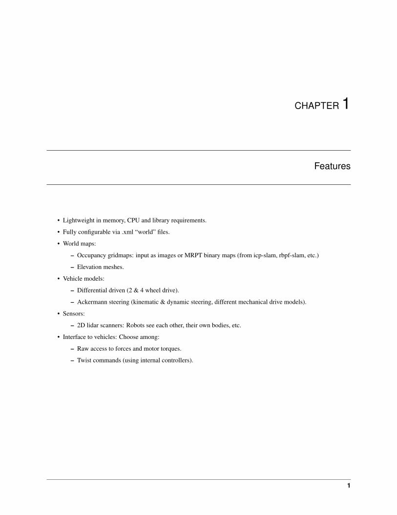
Features
• Lightweight in memory, CPU and library requirements.
• Fully configurable via .xml “world” files.
• World maps:
– Occupancy gridmaps: input as images or MRPT binary maps (from icp-slam, rbpf-slam, etc.)
– Elevation meshes.
• Vehicle models:
– Differential driven (2 & 4 wheel drive).
– Ackermann steering (kinematic & dynamic steering, different mechanical drive models).
• Sensors:
– 2D lidar scanners: Robots see each other, their own bodies, etc.
• Interface to vehicles: Choose among:
– Raw access to forces and motor torques.
– Twist commands (using internal controllers).
1

mvsim
2 Chapter 1. Features

CHAPTER 2
Installing
2.1 Build from sources
Dependencies:
• A decent C++17 compiler.
• CMake >= 3.1
• MRPT (>=2.0.0): In Windows, build from sources or install precompiled binaries.
• Box2D: Will use an embedded copy if no system version is found.
In Ubuntu, this will install all requirements:
sudo apt install \build-essential cmake g++ \libbox2d-dev \libmrpt-opengl-dev libmrpt-obs-dev libmrpt-maps-dev \libmrpt-gui-dev libmrpt-tfest-dev \protobuf-compiler \libzmq3-dev \pybind11-dev \libprotobuf-dev \libpython3-dev
Compile as usual:
mkdir buildcd buildcmake ..make#make test
3

mvsim
2.2 ROS: Compiling & usage
Either install as a precompiled package:
sudo apt install ros-$ROS_DISTRO-mvsim
Or build from sources, by cloning into a catkin workspace and build as usual.
Usage: See docs and tutorials in https://wiki.ros.org/mvsim
4 Chapter 2. Installing

CHAPTER 3
First steps
After installing or building from sources, you are ready to test the standalone simulator applications to get used toMVSIM.
3.1 1. Manual vehicle teleop
build/bin/mvsim-server mvsim_tutorial/mvsim_demo_2robots.xml
You should see the GUI of a demo world with two robots equipped with a 2D lidar, scanning a model defined bymeans of an occupancy grid map and a couple of boxes.
Use the keyboard to teleop the vehicle: w/s to increase/decrease the PI controller setpoint linear speed, and a/d toturn the Ackermann steering to the left/right. Use the spacebar as a brake.
Select the active robot by pressing the keys 1 or 2.
Note: The GUI of this program is likely to change soon.
5

mvsim
Fig. 1: Screenshot of the mvsim_demo_2robots example world.
6 Chapter 3. First steps
CHAPTER 4
Architecture
The project comprises:
• A C++ library: libmvsim
• A ROS1 node. It can be run standalone.
• mvsim-server: A standalone program to run the simulation and, optionally, displaying a GUI live view ofthe world, accept keyboard/mouse orders, etc. It also uses ZMQ+protobuf as a communication system for userprograms to interact with the simulation (for example, from a C++ or Python program).
7

mvsim
8 Chapter 4. Architecture

CHAPTER 5
Simulated world definition
Simulation happens inside a World object. This is the central class for usage from user code, running the simulation,loading XML models, managing GUI visualization, etc. The ROS node acts as a bridge between this class and theROS subsystem.
Simulated worlds are described via configuration files called “world” files, defined in the XML file format.
Many examples can be found in the mvsim_tutorial directory.
The next sections explain possible XML elements in a world file.
5.1 1. Global XML tags
World definition begins with tag <mvsim_world>. To define simulation timestep, use <simul_timestep> with floatvalue specified in seconds.
<mvsim_world version="1.0">...
<!-- General simulation options --><simul_timestep>0.005</simul_timestep> <!-- Simulation fixed-time interval
→˓for numerical integration [s] -->...</mvsim_world>
5.2 2. GUI options
GUI options are specified with tag gui. gui has several nested tags:
<mvsim_world version="1.0">...
<!-- GUI options -->
(continues on next page)
9

mvsim
(continued from previous page)
<gui><!-- Is camera orthographic or projective? --><ortho>false</ortho>
<!-- Show reaction forces on wheels with lines --><show_forces>true</show_forces><force_scale>0.01</force_scale> <!-- (Newtons to meters draw scale) --
→˓>
<!-- default camera distance in world units --><cam_distance>35</cam_distance>
<!-- camera vertical field of view in degrees --><fov_deg>35</fov_deg>
<!-- <follow_vehicle>r1</follow_vehicle> --></gui>
...</mvsim_world>
5.3 3. “World elements”
Scenario defines the “level” where the simulation takes place.
<element class=”occupancy_grid”> depicts MRPT occupancy map which can be specified with both image file(black and while) and MRPT grid maps. <file> specifies file path to image of the map.
<element class=”ground_grid”> is the metric grid for visual reference.
<element class=”elevation_map”> is an elevation map (!experimental). Mesh-based map is build of elevation mapin simple bitmap where whiter means higher and darker - lower.
This tag has several subtags:
• <elevation_image> - path the elevation bitmap itself
• <elevation_image_min_z> - minimum height in world units
• <elevation_image_max_z> - maximum height in world units
• <texture_image> - path texture image for elevation bitmap. Mus not be used with mesh_color simultaneously
• <mesh_color> - mesh color in HEX RGB format
• <resolution> - mesh XY scale
5.4 4. Vehicle class descriptions
Tag <vehicle:class> depictd description of vehicle class. The attribute name will be later referenced when describingvehicle exemplars.
Inside <vehicle:class> tag, there are tags <dynamics>, <friction> and exemplars of <sensor>.
10 Chapter 5. Simulated world definition

mvsim
5.4.1 Vehicle dynamics
At the moment, there are three types of vehicle dynamics implemented. Refer [vehicle_models] for more information.
<dynamics> with attribute class specifies class of dynamics used. Currently available classes:
• differential
• car_ackermann
• ackermann_drivetrain
Each class has specific inner tags structure for its own configuration.
5.4.2 Common
Every dynamics has wheels specified with tags <i_wheel> where i stand for wheel position index (r, l for differentialdrive and fr, fl, rl, rr for Ackermann-drive)
Wheel tags have following attributes:
• pos - two floats representing x an y coordinate of the wheel in local frame
• mass - float value for mass of the wheel
• width - float value representing wheel width [fig:wheel_forces]
• diameter - float value to represent wheel diameter [fig:wheel_forces]
Ackermann models also use <max_steer_ang_deg> to specify maximum steering angle.
<chassis> is also common for all dynamics, it has attributes:
• mass - mass of chassis
• zmin - distance from bottom of the robot to ground
• zmax - distance from top of the robot to ground
5.4.3 Controllers
There are controllers for every dynamics type [sec:controllers]. In XML their names are
• raw - control raw forces
• twist_pid - control with twist messages
• front_steer_pid - [Ackermann only] - control with PID for velocity and raw steering angles
Controllers with pid in their names use PID regulator which needs to be configured. There are tags <KP><KI><KD>for this purpose. Also they need the parameter <max_torque> to be set.
Twist controllers need to set initial <V> and <W> for linear and angular velocities respectively.
Steer controllers need to set initial <V> and <STEER_ANG> for linear velocity and steering angle respectively.
5.4.4 Ackermann-drivetrain model
needs a differential type and split to be configured. For this purpose there is a tag <drivetrain> with argument type.Supported types are defined in [sec:ackermann_drivetrain]. In XML their names are:
• open_front
5.4. 4. Vehicle class descriptions 11

mvsim
• open_rear
• open_4wd
• torsen_front
• torsen_rear
• torsen_4wd
<drivetrain> has inner tags describing its internal structure:
• <front_rear_split>
• <front_rear_bias>
• <front_left_right_split>
• <front_left_right_bias>
• <rear_left_right_split>
• <rear_left_right_bias>
which are pretty self-explanatory.
5.4.5 Friction
Friction models are described in [sec:friction_models] and defined outside of <dynamics>. The tag for friction is<friction> with attribute class.
Class names in XML are:
• wardiagnemma
• default
Default friction [sec:default_friction] uses subtags:
• <mu> - the friction coefficient
• <C_damping> - damping coefficient
In addition to default, Ward-Iagnemma friction includes subtags:
• A_roll
• R1
• R2
that are described in [sec:wi_friction].
5.4.6 Sensors
Sensors are defined with <sensor> tag. It has attributes type and name.
At the moment, only laser scanner sensor is implemented, its type is laser. Subtags are:
• <pose> - an MRPT CPose3D string value
• <fov_degrees> - FOV of the laser scanner
• <sensor_period> - period in seconds when sensor sends updates
• <nrays> - laser scanner rays per FOV
12 Chapter 5. Simulated world definition

mvsim
• <range_std_noise> - standard deviation of noise in distance measurements
• <angle_std_noise_deg> - standatd deviation of noise in angles of rays
• <bodies_visible> - boolean flag to see other robots or not
5.5 5. Vehicle instances
For each vehicle class, an arbitrary number of vehicle instances can be created in a given world.
Vehicle instances are defined with the <vehicle> tag that has attributes name and class. class must match one of theclasses defined earlier with <vehicle:class> tag.
Subtags are:
• <init_pose> - in global coordinates: 𝑥, 𝑦, 𝛾 (deg)
• <init_vel> - in local coordinates: 𝑣𝑥,𝑣𝑦 , 𝜔 (deg/s)
5.6 6. “Obstacle block” classes
Write me!
5.7 7. “Obstacle block” instances
Write me!
5.8 8. Vehicles and blocks parameters
Vehicles and obstacles blocks share common C++ mvsim::Simulable and mvsim::VisualObject interfacesthat provide the common parameters below.
Note: The following parameters can appear in either the {vehicle,block} class definitions or in a particular instantia-tion block, depending on whether you want parameters to be common to all instances or not, respectively.
5.8.1 Related to topic publication
Under the <publish> </publish> tag group:
• publish_pose_topic: If provided, the pose of this object will be published as a topic with message typemvsim_msgs::Pose.
• publish_pose_period: Period (in seconds) for the topic publication.
Example:
<publish><publish_pose_topic>/r1/pose</publish_pose_topic><publish_pose_period>50e-3</publish_pose_period>
</publish>
5.5. 5. Vehicle instances 13

mvsim
5.8.2 Related to visual aspect
Under the <visual> </visual> tag group:
• model_uri: Path to 3D model file. Can be any file format supported by ASSIMP, like .dae, .stl, etc. Ifempty, the default visual aspect will be used.
• model_scale: (Default=1.0) Scale to apply to the 3D model.
• model_offset_x, model_offset_y , model_offset_z: (Default=0) Offset translation [meters].
• model_yaw, model_pitch, model_roll: (Default=0) Optional model rotation [degrees].
• show_bounding_box: (Default=‘‘false‘‘) Initial visibility of the object bounding box.
Example:
<visual><model_uri>robot.obj</model_uri><model_scale>1.0</model_scale><model_offset_x>0.0</model_offset_x><model_offset_y>0.0</model_offset_y><model_offset_z>0.0</model_offset_z>
</visual>
14 Chapter 5. Simulated world definition

CHAPTER 6
Simulation execution
Simulation executes step-by-step with user-defined ∆𝑡 time between steps. Each step has several sub steps:
• Before time step - sets actions, updates models, etc.
• Actual time step - updates dynamics
• After time step - everything needed to be done with updated state
Each vehicle is equipped with parameters logger(s). This logger is not configurable and can be rewritten programmat-icaly.
Logger are implemented via CsvLogger class and make log files in CSV format which then can be opened via anyeditor or viewer.
Loggers control is introduced via robot controllers, each controller controls only loggers of its robot.
Best results in visualizing offers QtiPlot [fig:qtiplot_example1].
At the moment, following characteristics are logged:
• Pose (𝑥, 𝑦, 𝑧, 𝛼, 𝛽, 𝛾)
• Body velocity (�̇�, �̇�, �̇�)
• Wheel torque (𝜏 )
• Wheel weight (𝑚𝑤𝑝)
• Wheel velocity (𝑣𝑥, 𝑣𝑦)
Loggers support runtime clear and creating new session. The new session mode finalizes current log files and starts towrite to a new bunch of them.
• A limitation of box2d is that no element can be thinner than 0.05 units, or
the following assert will be raised while loading the world model:
15

mvsim
16 Chapter 6. Simulation execution

CHAPTER 7
Physic models
7.1 1. Wheel dynamics
We introduce wheels as a mass with cylindrical shape (Figure [fig:wheel_forces]). Each wheel has following proper-ties:
• location of the wheel as to the chassis ref point [m,rad] in local coordinates 𝐿𝑤 = {𝑥𝑤, 𝑦𝑤,Φ}
• diameter 𝑑𝑤 [m]
• width 𝑤𝑤 [m]
• mass 𝑚𝑤 [kg]
• inertia 𝐼𝑦𝑦
• spinning angular position 𝜑𝑤 [rad]
• spinning angular velocity 𝜔𝑤 [rad/s]
Thus, each wheel is represented as 𝑊 = {𝐿𝑤, 𝑑𝑤, 𝑤𝑤,𝑚𝑤, 𝐼𝑦𝑦, 𝜑𝑤, 𝜔𝑤}
Fig. 1: Wheel forces
7.2 2. Friction models
7.2.1 Friction models base
Friction model base introduces Friction input structure, that incorporates forces of wheel
• weight on this wheel from the car chassis, excluding the weight of the wheel itself 𝑤 [N]
• motor torque 𝜏 [Nm]
17

mvsim
• instantaneous velocity
𝜈 =
[︂𝜈𝑥𝜈𝑦
]︂in local coordinate frame
7.2.2 Default friction
At the moment, there is only one basic friction model available for vehicles. Default friction model evaluates . . .
Default friction evaluates forces in the wheel coordinate frame:
𝜈𝑤 =
[︂𝜈𝑤𝑥
𝜈𝑤𝑦
]︂= 𝑅(Φ𝑤) · 𝜈
To calculate maximal allowed friction for the wheel, we introduce partial mass:
𝑚𝑤𝑝 =𝑤𝑤
𝑔+ 𝑚𝑤
𝐹𝑓,𝑚𝑎𝑥 = 𝜇 ·𝑚𝑤𝑝 · 𝑔
Where 𝜇 is friction coefficient for wheel.
Calculating latitudinal friction (decoupled sub-problem):
𝐹𝑓,𝑙𝑎𝑡 = 𝑚𝑤𝑝 · 𝑎 = 𝑚𝑤𝑝 ·−𝜈𝑤𝑦
∆𝑡
𝐹𝑓,𝑙𝑎𝑡 = 𝑚𝑎𝑥(−𝐹𝑓,𝑚𝑎𝑥,𝑚𝑖𝑛(𝐹𝑓,𝑙𝑎𝑡, 𝐹𝑓,𝑚𝑎𝑥))
Calculating wheel desired angular velocity:
𝜔𝑐𝑜𝑛𝑠𝑡𝑟𝑎𝑖𝑛𝑡 =2𝜈𝑤𝑥
𝑑𝑤
𝐽𝑑𝑒𝑠𝑖𝑟𝑒𝑑 = 𝜔𝑐𝑜𝑛𝑠𝑡𝑟𝑎𝑖𝑛𝑡 − 𝜔𝑤
𝜔𝑑𝑒𝑠𝑖𝑟𝑒𝑑 =𝐽𝑑𝑒𝑠𝑖𝑟𝑒𝑑
∆𝑡
Calculating longitudinal friction:
𝐹𝑓,𝑙𝑜𝑛 =1
𝑅· (𝜏 − 𝐼𝑦𝑦 · 𝜔𝑑𝑒𝑠𝑖𝑟𝑒𝑑 − 𝐶𝑑𝑎𝑚𝑝 · 𝜔𝑤)
𝐹𝑓,𝑙𝑜𝑛 = 𝑚𝑎𝑥(−𝐹𝑓,𝑚𝑎𝑥,𝑚𝑖𝑛(𝐹𝑓,𝑙𝑜𝑛, 𝐹𝑓,𝑚𝑎𝑥))
Simply composing friction forces to vector:
𝐹𝑓 =
[︂𝐹𝑓,𝑙𝑎𝑡
𝐹𝑓,𝑙𝑜𝑛
]︂With new friction, we evaluate angular acceleration (code says angular velocity impulse, but the units are for acceler-ation) of the wheel:
𝛼 =𝜏 −𝑅 · 𝐹𝑓,𝑙𝑜𝑛 − 𝐶𝑑𝑎𝑚𝑝 · 𝜔𝑤
𝐼𝑦𝑦
Using given angular acceleration, we update wheel’s angular velocity:
𝜔𝑤 = 𝜔𝑤 + 𝛼 · ∆𝑡
18 Chapter 7. Physic models

mvsim
7.2.3 Ward-Iagnemma friction
This type of friction is an implementation of paper from Chris Ward and Karl Iagnemma :raw-latex:‘\cite{ward-iagnemma-friction}‘.
Rolling resistance is generally modeled as a combination of static- and velocity-dependant forces [17], [21]. Authorspropose function with form similar to Pacejka’s model :raw-latex:‘\cite{pacejka_tire_model}‘ as a continuouslydifferentiable formulation of the rolling resistance with the static force smoothed at zero velocity to avoid a singularity.The rolling resistance is
𝐹𝑟𝑟 = 𝑠𝑖𝑔𝑛(𝑉𝑓𝑤𝑑) ·𝑁 · (𝑅1 · (1𝑒𝐴𝑟𝑜𝑙𝑙|𝑉𝑓𝑤𝑑|) + 𝑅2 · |𝑉𝑓𝑤𝑑|)
Where 𝐴𝑟𝑜𝑙𝑙, 𝑅1, 𝑅2 are the model-dependent coefficients. The impact of these coefficients is shown at figure[fig:wi_rr] taken from original paper.
This force 𝐹𝑟𝑟 is then added to 𝐹𝑓,𝑙𝑜𝑛.
Default constants were chosen as in reference paper and showed good stability and robust results. In addition, theycan be altered via configuration file.
7.3 3. Vehicle models
Vehicle models are fully configurable with world XML files.
7.3.1 Vehicle base class
Vehicle base incorporates basic functions for every vehicle actor in the scene. It is also responsible for updating stateof vehicles.
It has implementation of interaction with world. Derived classes re-implement only work with torques/forces onwheels.
At the moment, no model takes into account the weight transfer, so weight on wheels is calculated in this base class.
Vehicle base class also provides ground-truth for velocity and position.
𝑝𝑤 =𝑝𝑐ℎ𝑎𝑠𝑠𝑖𝑠𝑁𝑤
• Before time step:
– Update wheels position using Box2D
– Invoke motor controllers (reimplemented in derived classes)
– Evaluate friction of wheels with passed friction model
– Apply force to vehicle body using Box2D
• Time step - update internal vehicle state variables 𝑞 and 𝑞
• After time step - updates wheels rotation
Center of mass is defined as center of Box2D shape, currently there is no +Z mobility.
7.3. 3. Vehicle models 19

mvsim
7.3.2 Differential driven
A differential wheeled robot is a mobile robot whose movement is based on two separately driven wheels placed oneither side of the robot body. It can thus change its direction by varying the relative rate of rotation of its wheels andhence does not require an additional steering motion.
Odometry-based velocity estimation is implemented via Euler formula (consider revising, it doesn’t include side slip):
𝜔𝑣𝑒ℎ =𝜔𝑟 ·𝑅𝑟 − 𝜔𝑙 ·𝑅𝑟
𝑦𝑟 − 𝑦𝑙
𝜈𝑥 = 𝜔𝑙 ·𝑅𝑙 + 𝜔 · 𝑦𝑙
𝜈𝑦 = 0
𝑊ℎ𝑒𝑟𝑒 : 𝑚𝑎𝑡ℎ : ‘𝜔𝑣𝑒ℎ‘𝑖𝑠𝑎𝑛𝑔𝑢𝑙𝑎𝑟𝑣𝑒𝑙𝑜𝑐𝑖𝑡𝑦𝑜𝑓𝑡ℎ𝑒𝑟𝑜𝑏𝑜𝑡,
𝑅𝑖 - radius of the wheel, 𝑦𝑖 is the y position of the wheel, 𝜔𝑖 is the angular velocity of the wheel. All calculations inthe robot’s local frame.
Nothing more interesting here.
7.3.3 Ackermann driven
Ackermann steering geometry is a geometric arrangement of linkages in the steering of a car or other vehicle designedto solve the problem of wheels on the inside and outside of a turn needing to trace out circles of different radii.
Ackermann wheels’ angles are computed as following:
𝛼𝑜𝑢𝑡𝑒𝑟 = 𝑎𝑡𝑎𝑛(𝑐𝑜𝑡(|𝛼| +𝑤
2𝑙)
𝛼𝑖𝑛𝑛𝑒𝑟 = 𝑎𝑡𝑎𝑛(𝑐𝑜𝑡(|𝛼| − 𝑤
2𝑙)
𝑤ℎ𝑒𝑟𝑒 : 𝑚𝑎𝑡ℎ : ‘𝛼‘𝑖𝑠𝑡ℎ𝑒𝑑𝑒𝑠𝑖𝑟𝑒𝑑𝑒𝑞𝑢𝑖𝑣𝑎𝑙𝑒𝑛𝑡𝑠𝑡𝑒𝑒𝑟𝑖𝑛𝑔𝑎𝑛𝑔𝑙𝑒,
𝑤 is wheels distance and 𝑙 is wheels base. Outer and inner wheel are defined by the turn direction.
Odometry-based velocity estimation is implemented via Euler formula (consider revising, it doesn’t include side slip):
𝜔𝑣𝑒ℎ =𝜔𝑟𝑟 ·𝑅𝑟𝑟 − 𝜔𝑟𝑙 ·𝑅𝑟𝑟
𝑦𝑟𝑟 − 𝑦𝑟𝑙
𝜈𝑥 = 𝜔𝑟𝑙 ·𝑅𝑟𝑙 + 𝜔 · 𝑦𝑟𝑙
𝜈𝑦 = 0
𝑊ℎ𝑒𝑟𝑒 : 𝑚𝑎𝑡ℎ : ‘𝜔𝑣𝑒ℎ‘𝑖𝑠𝑎𝑛𝑔𝑢𝑙𝑎𝑟𝑣𝑒𝑙𝑜𝑐𝑖𝑡𝑦𝑜𝑓𝑡ℎ𝑒𝑟𝑜𝑏𝑜𝑡,
𝑅𝑟𝑖 - radius of the rear wheel, 𝑦𝑟𝑖 is the y position of the rear wheel, 𝜔𝑟𝑖 is the angular velocity of the rear wheel. Allcalculations in the robot’s local frame.
7.3.4 Ackermann-driven with drivetrain
This type of dynamics has the same geometry as simple Ackermann-driven robots. However, its powertrain is com-pletely different.
Instead of one “motor” per wheel, this type of dynamics incorporates one “motor” linked to wheels by differentials.
There are two types of differentials:
20 Chapter 7. Physic models

mvsim
• Open differntial
• Torsen-like locking differential :raw-latex:‘\cite{torsen-whitepaper}‘
Each type of differential can be linked with following configurations:
• Front drive
• Rear drive
• 4WD
Split is customizable between all axes.
As engine plays controller, whose torque output is then fed into differentials.
For open differential act the following equations:
𝜏𝐹𝐿 = 𝜏𝑚𝑜𝑡𝑜𝑟 ·𝐾𝑠,𝑓 ·𝐾𝑠,𝑓𝑟𝑙
𝜏𝐹𝑅 = 𝜏𝑚𝑜𝑡𝑜𝑟 ·𝐾𝑠,𝑓 · (1 −𝐾𝑠,𝑓𝑟𝑙)
𝜏𝑅𝐿 = 𝜏𝑚𝑜𝑡𝑜𝑟 ·𝐾𝑠,𝑟 ·𝐾𝑠,𝑟𝑟𝑙
𝜏𝑅𝑅 = 𝜏𝑚𝑜𝑡𝑜𝑟 ·𝐾𝑠,𝑟 · (1 −𝐾𝑠,𝑓𝑟𝑙)
Where 𝐾𝑠,𝑓 ,𝐾𝑠,𝑓𝑟𝑙,𝐾𝑠,𝑟𝑟𝑙 are split coefficients between axes.
Different things happen for Torsen-like differentials. As this type is self-locking, its torque output per wheel dependson wheel’s velocity. Here is the function of selecting torque on the next time step based on previous time step velocity.First, introduce the bias ratio - the ratio indicating how much more torque the Torsen can send to the tire with moreavailable traction, than is used by the tire with less traction. This ratio represents the “locking effect” of the differential.By default, it is set to 𝑏 = 1.5
𝜔1, 𝜔2 and 𝑡1, 𝑡2 are the output axles angular velocities and torque splits respectively. 𝐾𝑠 is differential split when itis not locked.
𝜔𝑚𝑎𝑥 = 𝑚𝑎𝑥(|𝜔1|, |𝜔2|)
𝜔𝑚𝑖𝑛 = 𝑚𝑖𝑛(|𝜔1|, |𝜔2|)
𝛿𝑙𝑜𝑐𝑘 = 𝜔𝑚𝑎𝑥 − 𝑏 · 𝜔𝑚𝑖𝑛
𝛿𝑡 =
{︃𝛿𝑙𝑜𝑐𝑘 · 𝜔𝑚𝑎𝑥, if 𝛿𝑙𝑜𝑐𝑘 > 0
0, if 𝛿𝑙𝑜𝑐𝑘 ≤ 0
𝑓1 =
{︃𝐾𝑠 · (1 − 𝛿𝑡) if |𝜔1| − |𝜔2| > 0
𝐾𝑠 · (1 + 𝛿𝑡)
𝑓2 =
{︃(1 −𝐾𝑠) · (1 + 𝛿𝑡) if |𝜔1| − |𝜔2| > 0
(1 −𝐾𝑠) · (1 − 𝛿𝑡)
𝑡1 =𝑓1
𝑓1 + 𝑓2
𝑡2 =𝑓2
𝑓1 + 𝑓2
Torque delivery for 2WD is pretty straightforward. There is one input from “motor” and two outputs to wheels, sowheel torques are:
𝜏𝑖 = 𝜏𝑚𝑜𝑡𝑜𝑟 · 𝑡𝑖
7.3. 3. Vehicle models 21

mvsim
where 𝑡𝑖 is the output of Torsen differential for 𝑖-th wheel.
With 4WD, torque is first split with Torsen to front and rear parts, each of them is than split independently with anotherTorsen.
At the moment, there is no model of the engine and thus no feedback of tires torque to engine.
7.4 4. Controllers
Different vehicles have different controllers. At the moment, differential and Ackermann drives have their own con-trollers.
Controllers are divided into several types:
• Raw forces
• Twist
Ackermann has controller, which controls steering angle and speed.
Controllers’ input and output are described by dynamics’ classes that they use.
7.4.1 Differential raw controller
This type of controller has simple response to user’s input integrating wheel torque with each simulation frame.
7.4.2 Differential Twist controller
Differential twist controller uses PID regulator to control linear and angular speed of the robot.
Setpoints for 𝑣𝑟 and 𝑣𝑙 are calculated as following:
𝑣𝑙 = 𝜈 − 𝜔
2· 𝑤
𝑣𝑟 = 𝜈 +𝜔
2· 𝑤
where 𝜈 is desired linear velocity and 𝜔 is desired angular velocity.
Inverted formula are suitable to get actual velocities from odometry estimates.
Then, velocity of the wheels is controlled with PID regulator.
7.4.3 Ackermann raw controller
As a raw differential controller, raw Ackermann controller integrates user input and sets wheel torques and steeringwheel angle.
7.4.4 Ackermann twist controller
Ackermann twist controller uses PID regulator to control wheel torques responding to angular and linear velocitycommands. Turn radius and desired steering angle are calculated:
𝑅 =𝜈𝑠𝜔𝑠
22 Chapter 7. Physic models

mvsim
𝛼 = 𝑎𝑡𝑎𝑛(𝑤
𝑟)
Desired velocities for wheels are computed by rotating desired linear velocity to the steering angle. In the same way,actual velocities from “odometry” are computed.
Then, torque of separate wheels is controlled with PID regulators for each wheel.
7.4.5 Ackermann steering controller
Ackermann steering controller takes as input linear speed an steering angle.
Then, it executes Ackermann twist controller to control wheels’ torques.
7.4.6 Ackermann-drivetrain controllers
These controllers’ steering is identical to Ackermann contollers, however, their torque part is different.
These controllers’ output acts like ’engine’ for drivetrain. Instead of separate outputs to wheels, it has one torqueoutput to differentials that will split it to separate wheels.
7.4. 4. Controllers 23

mvsim
24 Chapter 7. Physic models

CHAPTER 8
Extensions
It is possible to extend the simulator with custom models for sensors, vehicles, and world elements.
Note: Write me!
25

mvsim
26 Chapter 8. Extensions

CHAPTER 9
About
Lightweight, realistic dynamical simulator for 2D (“2.5D”) vehicles and robots. It is tailored to analysis of vehicledynamics, wheel-ground contact forces and accurate simulation of typical robot sensors (e.g. laser scanners).
This project includes a C++ library mvsim, a standalone app, and a ROS1 node.
Licensed under the permissive 3-clause BSD License.
Documentation credits:
• Borys Tymchenko @spsancti
• Jose Luis Blanco Claraco @jlblancoc
Github repository: https://github.com/MRPT/mvsim
27

mvsim
28 Chapter 9. About

CHAPTER 10
Indices and tables
• genindex
• modindex
• search
29


