My data are incomplete and noisy: Information-reduction statistical methods for knowledge extraction...

INTRODUCTION GOAL INCOMPLETE DATA STOCHASTIC MODELLING SYNTHETIC LIKELIHOODS ABC SUMMARY

My data are incomplete and noisy!

Information-reduction statistical methods for knowledgeextraction can save your day: tools and opportunities for

modelling

Docent/Readership lectureLund, 7 June 2016

Umberto PicchiniCentre for Mathematical Sciences

Lund Universitywww.maths.lth.se/matstat/staff/umberto/

June 7, 2016

1 / 54

www.maths.lth.se/matstat/staff/umberto/


PREAMBLE: WHAT IS A DOCENT/READERSHIP

LECTURE?

It’s a lecture in a popular science context.

Target are research students within the entire Faculty of Scienceat Lund University.

It should cover my own subject area, but not my own researchoutput.

My notation and level of exposition will be subject to the above.

2 / 54


I will discuss a few methods for parameter inference (akacalibration, inverse problem) in presence of incomplete andnoisy data.

However I will start mentioning:

I what I mean with incomplete and noisy observations;

I why use stochastic modelling;

I issues with state-of-art inference methods for dynamicmodels.

I will focus on two methods based on information reductionthat use summary statistics of data: synthetic likelihoods andapproximate Bayesian computation.

These are powerful, general and flexible methods but also veryeasy to introduce to a general audience of researchers.

3 / 54


Goal is to show how state-of-art exact methods for parameterestimation can spectacularly fail in some scenarios, including:

I near chaotic systems;

I noisy (stochastic) dynamical systems;

I badly initialized optimization or Bayesian MCMCalgorithms.

But first, what do I mean with “incomplete data”?

4 / 54


INCOMPLETE OBSERVATIONS

There can be many situations where we only have partialinformation of the system of scenario of interest.

We oversimplify and call “incomplete” or “partially observed”those experiments where not all the variables of interest areobservable.

This could mean that at least one of the following holds:

1. some variables are completely unobserved (measurementsfor those variables are unavailable)

2. we have a system evolving continuously in time but weonly observe it a discrete time points;

3. the variables we observe are perturbed measurements ofthe actual variables of interest.

5 / 54


Consider a noise perturbed “signal”

Typically values of our measurements do not exclusivelyrepresent what we are really interested in measuring.

The unperturbed signal is unavailable because measurementsare corrupted with noise.

6 / 54


Therefore we have a system (think about a physical system)having

I an observable component Y

I an unobservable/latent signal X

I noise ε

And of course if we model time dynamics we could think of ndiscrete-time measurements

Yti = Xti + εti , i = 1, ...,n

Or more in general

Yti = f (Xti , εti)

for some arbitrary yet known function f (·).

7 / 54


AN EXAMPLE: CONCENTRATION OF A DRUG

Time course of a certain drug concentration in blood. This ismeasured at discrete times.

**

*

** *

** * *

0 20 40 60 80 100 120

020

4060

8010

0

time in minutes

C12

con

cent

ratio

n

8 / 54


We may postulate a deterministic model:

dCt

dt= −µCt

Ct = C0e−µt, µ > 0

With measurements Yti = Cti + εti , with εti ∼ N (0, σ2ε)

**

*

** *

** * *

0 20 40 60 80 100 120

020

4060

8010

0

time in minutes

C12

con

cent

ratio

n

There’s some discrepancy with thefit (residual error).

9 / 54


We may postulate a deterministic model:

dCt

dt= −µCt

Ct = C0e−µt, µ > 0

With measurements Yti = Cti + εti , with εti ∼ N (0, σ2ε)

**

*

** *

** * *

0 20 40 60 80 100 120

020

4060

8010

0

time in minutes

C12

con

cent

ratio

n

There’s some discrepancy with thefit (residual error).

9 / 54


In previous slides you might have noticed the introduction of aparameter µ > 0.

Even though an expert researcher might have a clue aboutsome reasonable value for µ, in reality this is at best nothingmore than a guess.

In fact, when we previously wrote that we can assume

Yti = f (Xti , εti) = f (Cti , εti)

most often what we have is

Yti = f (Xti , θ, εti) = f (Cti , µ, εti)

that is a dependence from an unknown (vector) parameter θ.

In our example θ ≡ µ.

10 / 54


My main interest:to study and develop principled methods that return anestimate of θ and its uncertainty analysis.

In particular, I am interested in modelling stochastic dynamics.

In the previous example Ct was evolving in a deterministicfashion, given a fixed starting value C0 and a fixed value for µ.

In next slide I show an alternative, stochastic approach.

11 / 54


Add systemic (white) noise:

dC(t)dt

= −µC(t) + “white noise”

And again Yti = Cti + εti , with εti ∼ N (0, σ2ε)

**

*

** *

** * *

0 20 40 60 80 100 120

020

4060

8010

0

time in minutes

C12

con

cent

ratio

n

Dynamics are stochastic.Residual error can’t be eliminated.It’s always “there”.

12 / 54


Add systemic (white) noise:

dC(t)dt

= −µC(t) + “white noise”

And again Yti = Cti + εti , with εti ∼ N (0, σ2ε)

**

*

** *

** * *

0 20 40 60 80 100 120

020

4060

8010

0

time in minutes

C12

con

cent

ratio

n

Dynamics are stochastic.Residual error can’t be eliminated.It’s always “there”.

12 / 54


The problem with stochastic models is that:

1. realizations from the model might not really resemble theobserved data...

2. this can happen even when simulate using a θ which isclose to its true value...

3. ...and even when we are simulating from the “true model”(simulation studies).

Although this is understandable, it is also upsetting when ourmethods are based on producing realizations meant to get closeto observations.

13 / 54


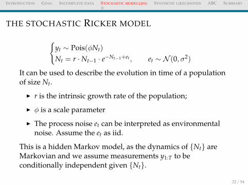
A NEARLY CHAOTIC MODELTwo realizations from the Ricker model (discussed later), withoutmeasurement noise.

Nt = r ·Nt−1 · e−Nt−1+et , et ∼ N (0, σ2)

Small changes in a parameter cause major departures from data.0

510

15n t

Time5 10 15 20 25 −2

60−2

20−1

80−1

40Lo

g−lik

elih

ood

log(r)2.5 3.0 3.5 4.0 4.5

Figure: One path generated with log r = 3.8 (black) and one generated withlog r = 3.799 (red) when σ = 0.

14 / 54


I Now, a modeller (say a statistician) does not necessarilyhave the expertise nor the time to study the qualitativebehaviour of solutions of a series of candidate models.

I most often the modeller wants to test a range of possiblemodels against available data.

I Simulations from postulated models should producetrajectories approximately resembling data.

I Parameter estimation should be performed to identify“best fitting” parameters.

15 / 54


Notice for many years even simple stochastic models have beenterribly difficult to calibrate against data.

It is usually impossible to write the likelihood function p(y1:T|θ)in closed form.

It is also impossible to write filtering densities for the statesp(x1:T|y1:T; θ).

Notation:

I I am going to use lower case letters both for randomvariables and for their realized values.

I I use a1:T to denote a sequence (a1, a2, ..., aT) where T is thetime horizon.

I I assume integer time indeces to ease notation.

16 / 54


SSM: STATE–SPACE MODELGraphically:

"!# "!# "!#

"!# "!# "!#

Yt−1 Yt Yt+1

Xt−1 Xt Xt+1- - - -

6 6 6

... ... (Markov chain)

(Observations)

(Yt|Xt = xt) ∼ p(yt|xt) (Observation density)(Xt+1|Xt = xt) ∼ p(xt+1|xt) (Transition density)

X0 ∼ π(x0) (Initial distribution)

Example: Yt a subject’s measured glycemia at time t. Xt theactual glycemia at t.

17 / 54


THE LIKELIHOOD FUNCTION 1/2

It turns out that, even for such a simple construct, it is difficultto write the likelihood function.

In a SSM data are not independent, they are only conditionallyindependent→ complication!:

p(y1:T|θ) = p(y1|θ)T∏

t=2

p(yt|y1:t−1, θ) =?

We don’t have a closed for expression for the product abovebecause we do not know how to calculate p(yt|y1:t−1, θ).

Let’s see why.

18 / 54


THE LIKELIHOOD FUNCTION 2/2In a SSM the observed process is assumed to depend on the latentMarkov process {Xt}: we can write

p(y1:T|θ) =

∫p(y1:T, x0:T|θ)dx0:T =

∫p(y1:T|x0:T, θ)︸︷︷︸use cond. indep.

× p(x0:T|θ)︸︷︷︸use Markovianity

dx0:T

=

∫ T∏

t=1

p(yt|xt, θ)×{

p(x0|θ)T∏

t=1

p(xt|xt−1, θ)

}dx0:T

Problems

I The expression above is a (T + 1)-dimensional integral /

I For most (nontrivial) models, transition densities p(xt|xt−1) areunknown /

19 / 54


However today we have quite a number of reliable Monte Carlosolutions to the integration problem.

I am not going to introduce state-of-art methods for SSM but theseare essentially based on particle filters (or sequential Monte Carlo)methods.

I particle marginal methods and particle MCMC (Andrieu andRoberts 2009; Andrieu et al. 2010) for Bayesian inference.

I iterated filtering (Ionides et al. 2011, 2015) for maximumlikelihood inference.

As shown in Andrieu and Roberts 2009:

1. obtain an approximation of the likelihood p(y1:T|θ) using particlefilters;

2. plug p(y1:T|θ) into a MCMC algorithm for Bayesian inference onθ.

3. then the MCMC returns samples exactly from π(θ|y1:T).

20 / 54


If you are interested in a quick review of particle methods forparameters inference (not state inference) check my slides onSlideShare http://goo.gl/4aZxL1

As I said in this presentation I focus on synthetic likelihoodsand approximate Bayesian computation.

I now consider a simple example where the celebrated particlemarginal methodology of Andrieu and Roberts1, which issupposed to return exact Bayesian inference, does not work.

1C. Andrieu and G. Roberts 2009, Annals of Statistics 37(2).21 / 54

http://goo.gl/4aZxL1


THE STOCHASTIC RICKER MODEL

{yt ∼ Pois(φNt)

Nt = r ·Nt−1 · e−Nt−1+et , et ∼ N (0, σ2)

It can be used to describe the evolution in time of a populationof size Nt.

I r is the intrinsic growth rate of the population;

I φ is a scale parameter

I The process noise et can be interpreted as environmentalnoise. Assume the et as iid.

This is a hidden Markov model, as the dynamics of {Nt} areMarkovian and we assume measurements y1:T to beconditionally independent given {Nt}.

22 / 54


Here is a realization of length T = 50 from the Ricker model.

050

150

250

y

05

1015

2025

N

−0.

40.

00.

20.

4

0 10 20 30 40 50

e

time

myobservedricker

Ground-truth parameters are log r = 3.8, φ = 10 and σ = 0.3 (andimposing N0 = 7 and e0 = 0). Same settings as in S. Wood 20102

2S. Wood 2010, Nature 466, pp. 1102–1104.23 / 54


SOFTWARE CODE

The simulation results in the next three slides can bereproduced using the code athttps://github.com/umbertopicchini/pomp-ricker

24 / 54

https://github.com/umbertopicchini/pomp-ricker


RUNNING pomp ricker− pmcmc.R FOR EXACT BAYESIAN INFERENCE

Suppose we are only interested in estimating the parameter r fromdata, while remaining quantities are fixed to their ground-truthvalues.

Particle MCMC works well here. So exact inference is possible.

Here is an MCMC chain of length 2000 with likelihood estimated viabootstrap filter (1000 particles used). We let r start at r = 12.2.

True value is r = 44.7, estimated posterior mean is 44.6 [38.5,51.7]

0 500 1000 1500 2000

2030

4050

Iterations25 / 54


So all good in the considered example.

We might reasonably imagine that if our model is “lessstochastic” (a smaller σ) it should be even easier to conductinference.

Recall that

Nt = r ·Nt−1 · e−Nt−1+et , et ∼ N (0, σ2)

Modellers don’t know a-priori the values of underlyingparameters.

Suppose we now use data generated with σ = 0.01 (instead ofσ = 0.3)

26 / 54


Here is what happens with the same conditions as before,except for using data generated with σ = 0.01.

−12

00−

1050

−90

0

logl

ik

−7

−6

−5

−4

−3

log.

prio

r

1214

1618

nfai

l

1315

17

r

0 500 1000 1500 2000

PMCMC iteration

PMCMC convergence diagnostics

The chain (lower panel) is stuck at the wrong mode! r ≈ 18hence log r = 2.9.

It gets stuck even if we use more particles. 27 / 54


As beautifully illustrated in Fasiolo et al.3, the very interesting reasonwhy the estimation fails for nearly deterministic dynamics is thefollowing:

2.0 2.5 3.0 3.5 4.0 4.5

−1

20

−1

10

−1

00

−9

0−

80

σ = 0.3

2.0 2.5 3.0 3.5 4.0 4.5

−1

40

−1

20

−1

00

−8

0

σ = 0.1

2.0 2.5 3.0 3.5 4.0 4.5

−1

40

−1

20

−1

00

−8

0

σ = 0.05

2.0 2.5 3.0 3.5 4.0 4.5

−1

80

−1

40

−1

00

σ = 0.01

Lo

g−

like

liho

od

log(r)

Figure: Black: the true likelihood for log r. Red: the particle filterapproximation. Figure from Fasiolo et al. 2016.

3M. Fasiolo, N. Pya and S. Wood 2016. Statistical Science 31(1),pp. 96-11828 / 54


However the filter being unable to approximate the likelihood is onlyconsequence of something more subtle: look at the exact loglikelihoodfor non-stochastic dynamics, i.e. here σ = 0.

2.5 3.0 3.5 4.0

−15

−10

−5

Ricker

log(r)

27

12

17

nt

−5 −4 −3 −2

−35

−25

−15

−5

0

Pennycuick

log(a)

0.5 1.0 1.5 2.0

−1

5−

10

−5

0

Varley

log(b)0.0 0.5 1.0 1.5 2.0 2.5 3.0 3.5

−15

−10

−5

Maynard−Smith

log(r)

Log−

likelih

ood (

10

3)

Figure: Black: the true loglikelihood when σ = 0. Grey: bifurcation diagram.Figure from Fasiolo et al. 2016.

Go here if you are unfamiliar with bifurcations.29 / 54

http://mathforum.org/mathimages/index.php/Logistic_Bifurcation


The instability of some models for a small quantity of noise (σ)produces major differences in simulated trajectories for smallperturbations in the parameters.

05

1015

n t

Time5 10 15 20 25 −2

60−2

20−1

80−1

40Lo

g−lik

elih

ood

log(r)2.5 3.0 3.5 4.0 4.5

Figure: One path generated with log r = 3.8 (black) and one generated withlog r = 3.799 (red) when σ = 0.

30 / 54


A CHANGE OF PARADIGM

from S. Wood, Nature 2010:

“Naive methods of statistical inference try to make the modelreproduce the exact course of the observed data in a way that the realsystem itself would not do if repeated.”

“What is important is to identify a set of statistics that is sensitive tothe scientifically important and repeatable features of the data, butinsensitive to replicate-specific details of phase.”

In other words, with complex, stochastic and/or chaotic modelwe should try to match features of the data, not the path of thedata themselves.

31 / 54


SYNTHETIC LIKELIHOODS

I y: observed data, from static or dynamic models

I s(y): (vector of) summary statistics of data, e.g. mean,autocorrelations, marginal quantiles etc.

I assumes(y) ∼ N (µθ,Σθ)

an assumption justifiable via second order Taylorexpansion (same as in Laplace approximations).

I µθ and Σθ unknown: estimate them via simulations.

32 / 54

INTRODUCTION GOAL INCOMPLETE DATA STOCHASTIC MODELLING SYNTHETIC LIKELIHOODS ABC SUMMARYnature09319-f2.2.jpg (JPEG Image, 946 × 867 pixels) - Scaled (84%) http://www.nature.com/nature/journal/v466/n7310/images/nature09319...

1 of 1 29/05/2016 16:03

Figure: Schematic representation of the synthetic likelihoods procedure.33 / 54


I For fixed θ we simulate Nr artificial datasets y∗1 , ..., y∗Nr

andcompute corresponding (possibly vector valued) summariess∗1 , ..., s

∗Nr

.

I compute

µθ =1

Nr

Nr∑

i=1

s∗i , Σθ =1

Nr − 1

Nr∑

i=1

(s∗i − µθ)(s∗i − µθ)′

I compute the statistics sobs for the observed data y.

I evaluate a multivariate Gaussian likelihood at sobs

liks(θ) := exp(ls(θ)) = N (sobs; µθ, Σθ) ∝1√|Σθ|

e−(sobs−µθ)Σ−1θ (sobs−µθ)/2

I This likelihood can be maximized for a varying θ or be pluggedwithin an MCMC algorithm for Bayesian inferenceπ(θ|sobs) ∝ liks(θ)π(θ).

34 / 54


For the Ricker model Wood (2010) uses 13 summaries,including:

I the sample mean of observations y;

I number of zeros in the dataset;

I autocovariances up to lag 5;

I estimates for β0 and β1 from fitting

E(y0.3t ) = β0y0.3

t−1 + β1y0.6t−1

I and a few more summaries...(not important to bementioned here, but you got the idea).

So we have sobs = (y,#zeros, autocovars, β0, β1, ...).

35 / 54


RUNNING pomp ricker− synlik.R

We consider the dataset generated with the settings whereparticle methods have failed (same starting values etc.), i.e.σ = 0.01.

Here follow synthetic likelihood estimates:

r σ φ

starting value 12.18 1 20true value 44.7 0.01 10

SL estimate 45.25 0.23 10.16

We maximised liks(θ) using Nelder–Mead with Nr = 5000simulations.Standard errors could be found via profile likelihood (notreported).

36 / 54


BAYESIAN SYNTHETIC LIKELIHOODSJust plug liks(θ) in a Metropolis-Hastings MCMC procedure tosample from π(θ|sobs) ∝ liks(θ)π(θ).

Figure is from Price et al. (2016). They consider the “nicelybehaved” data obtained with σ = 0.3.

Table 3: Sensitivity of BSL/uBSL to n for the Ricker example with regards to MCMCacceptance rate, normalised ESS for each parameter and standard deviation of the esti-mated log SL at θ = (3.8, 10, 0.3)>. A ‘-’ indicates that a result is not available for uBSLas the value of n is too small.n acc. rate (%) ESS log r ESS σe ESS φ sd

(log pA,n(y|θ = (3.8, 10, 0.3)>)

)

20 2.4/1.8 11/8 13/10 18/13 large30 8.2/7.7 23/22 27/25 38/31 4.140 12.5/12.6 29/28 34/32 44/42 2.550 15.9/15.7 30/31 35/35 45/45 1.980 21.8/21.4 29/29 34/32 47/47 1.2100 24.1/23.7 25/27 30/30 41/39 1.0250 29.6/29.5 13/14 15/17 20/23 0.6

3 3.5 4 4.50

1

2

n=30n=100n=250

(a) log r

8 10 120

0.2

0.4

0.6

0.8

n=30n=100n=250

(b) φ

-0.2 0 0.2 0.4 0.60

1

2

3

4

n=30n=100n=250

(c) σe

Figure 6: Posterior estimates for log r, σe and φ of the Ricker model when using BSL withvarious values of n.

3 3.5 4 4.50

1

2

n=30n=100n=250

(a) log r

8 10 120

0.2

0.4

0.6

0.8

n=30n=100n=250

(b) φ

-0.2 0 0.2 0.4 0.60

1

2

3

4

n=30n=100n=250

(c) σe

Figure 7: Posterior estimates for log r, σe and φ of the Ricker model when using uBSLwith various values of n.

18

Figure: Posteriors for several values of Nr. True parameter values are:log r = 3.8, φ = 10, σ = 0.3 37 / 54

http://eprints.qut.edu.au/92795/


APPROXIMATE BAYESIAN COMPUTATION (ABC)

Another methodology, also using information-reduction viasummaries, is Approximate Bayesian Computation (ABC).

ABC has received enormous interest. A list of review papers isprovided in the references section.

You can also check my own intro to ABC.

38 / 54

http://www.slideshare.net/UmbertoPicchini/intro-to-approximate-bayesian-computation-abc


LIKELIHOOD FREE REJECTION SAMPLING

Recall y is data.

We wish to sample from π(θ|y) ∝ p(y|θ)π(θ).

1. simulate from the prior θ∗ ∼ π(θ)

2. plug θ∗ in your model and simulate artificial data y∗ [thisis the same as writing y∗ ∼ p(y|θ∗)]

3. if y∗ = y store θ∗. Go to step 1 and repeat.

The above is a likelihood free algorithm: it does not requireknowledge of the expression of the likelihood p(y|θ).

Each accepted θ∗ is such that θ∗ ∼ π(θ|y) exactly.

39 / 54


ABC REJECTION (PRITCHARD ET AL.4)

Same as before, but comparing s(y) with s(y∗) for “appropriate”summaries s(·) and a small tolerance ε > 0.

1. simulate from the prior θ∗ ∼ π(θ)

2. simulate a y∗ ∼ p(y|θ∗), compute s(y∗)

3. if ‖ s(y∗)− s(y) ‖< ε store θ∗. Go to 1 and repeat.

Samples are from πε(θ|s(y)) with

πε(θ|s(y)) ∝∫

Yp(y∗|θ∗)π(θ∗)IAε,y(y∗)dy∗

Aε,y(y∗) = {y∗ ∈ Y; ‖ s(y∗)− s(y) ‖< ε}.

4Pritchard et al. 1999, Molecular Biology and Evolution, 16:1791-1798.40 / 54


EXAMPLE: g-AND-k DISTRIBUTIONS

I Mixtures of Gaussians are often used to describe complex,nonstandard distributions.

I a mixture of two-Gaussians requires specifying 5parameters.

I apparently, it is sometimes challenging to estimate suchparameters due to unidentifiability (Marin and Robert5).

I simulating (sampling) from mixtures is an optimizationproblem (can be computer intensive).

5Marin and Robert, Bayesian Core, Springer 2007.41 / 54


g-and-k distributions only require 4 parameters and it’s fast tosimulate from them.

g-and-k distributions have no closed-form likelihood, but we cansimulate their quantiles.

F−1(x; A,B, g, k) = A + B[

1 + 0.8 · 1− exp(−g · r(x))

1 + exp(−g · r(x))

](1 + r2(x))kr(x)

with r(x) ∼ N(0, 1) the xth quantile from a standard Gaussian.

data0 5 10 15 20 25 30

0

500

1000

1500

2000

2500

3000

3500

4000

4500

n = 10, 000 samples generated with A = 3, B = 1, g = 2, k = 0.5.42 / 54


I wrote an MCMC algorithm using ABC with summaries the20th, 40th, 60th, 80th empirical quantiles and the skewnessvalue

s(y) = (q20, q40, q60, q80, skew(y)).

Again, we simulate datasets y∗, compute s(y∗) and comparethem with s(y) at each MCMC iteration.

I let the threshold ε decrease progressively during thealgorithm.

43 / 54


Red lines are true parameter values.

A ×104

0 1 2 3 4 5 62.5

3

3.5

4

4.5

5

B ×104

0 0.5 1 1.5 2 2.5 3 3.5 4 4.5 50

1

2

3

4

5

6

g ×104

0 0.5 1 1.5 2 2.5 3 3.5 4 4.5 50

2

4

6

8

10

k ×104

0 0.5 1 1.5 2 2.5 3 3.5 4 4.5 50

0.5

1

1.5

2

It is evident that I reduced ε at iteration 10,000 and then atiteration 20,000.

44 / 54


SUMMARY

I We have discussed plug-and-play methods that only require theability to simulate from the model.

I How to choose summaries s(·) is a delicate and open problem.

I However there exist much literature available.

I Information-reduction methods are very general and in manycases are the only possible option for inference.

I ABC and SL can be used for a short pilot run, to obtain a betterstarting value for θ to be used in more accurate methods.

I For example Owen et al.6 use ABC to obtain a starting value forparticle MCMC.

6Owen et al. 2015. Likelihood free inference for Markov processes: acomparison. Statistical applications in genetics and molecular biology, 14(2),pp.189-209.

45 / 54


Our suggestion, when dealing with a new model or a newdataset, is not to settle on a single methodology, but insteadtry to perform a battery of algorithms.

This require method developers to share their software codes toease methods reproducibility.

This is still not common practice.

46 / 54


If you wish to review some of the presented concepts, slides for thispresentation are available on SlideShare athttp://goo.gl/gg0Cqq.

R code to reproduce the Ricker model results is athttps://github.com/umbertopicchini/pomp-ricker/

MATLAB code for ABC and g-and-k distributions is athttps://github.com/umbertopicchini/abc_g-and-k/

Feel free to write me or drop by7 for a chat.

Thank You

[email protected], office MH:321, Matematikcentrum47 / 54

http://goo.gl/gg0Cqq

https://github.com/umbertopicchini/pomp-ricker/

https://github.com/umbertopicchini/abc_g-and-k/


If you wish to review some of the presented concepts, slides for thispresentation are available on SlideShare athttp://goo.gl/gg0Cqq.

R code to reproduce the Ricker model results is athttps://github.com/umbertopicchini/pomp-ricker/

MATLAB code for ABC and g-and-k distributions is athttps://github.com/umbertopicchini/abc_g-and-k/

Feel free to write me or drop by7 for a chat.

Thank [email protected], office MH:321, Matematikcentrum

47 / 54

http://goo.gl/gg0Cqq

https://github.com/umbertopicchini/pomp-ricker/

https://github.com/umbertopicchini/abc_g-and-k/


REFERENCES ON SYNTHETIC LIKELIHOODS

1. Fasiolo, M., Pya, N. and Wood, S.N., 2016. A Comparison ofInferential Methods for Highly Nonlinear State Space Models inEcology and Epidemiology. Statistical Science, 31(1), pp.96-118.

2. Meeds, E. and Welling, M., 2014. GPS-ABC: Gaussian processsurrogate approximate Bayesian computation. arXiv:1401.2838.

3. Price, L.F., Drovandi, C.C., Lee, A. and Nott, D.J., 2016. Bayesiansynthetic likelihood. http://eprints.qut.edu.au/92795/

4. Wood, S.N., 2010. Statistical inference for noisy nonlinearecological dynamic systems. Nature, 466(7310), pp.1102-1104.

(4) is where SL got first introduced. Our talk is largely based on (1).(2) merges SL with ABC. (3) studies the performance of SL in a(pseudo-marginal) Bayesian setting.

48 / 54

http://eprints.qut.edu.au/92795/


SOFTWARE FOR SYNTHETIC LIKELIHOODS

I R package pomp: http://kingaa.github.io/pomp

I R package synlik:https://mfasiolo.github.io/synlik_release/

49 / 54

http://kingaa.github.io/pomp

https://mfasiolo.github.io/synlik_release/


ABC SOFTWARE

I EasyABC, R package. Research article.

I abc, R package. Research article

I abctools, R package. Research article. Focusses on tuning.

I Lists with more options here and here .

I examples with implemented model simulators (useful toincorporate in your programs).

50 / 54

https://cran.r-project.org/web/packages/EasyABC/index.html

http://onlinelibrary.wiley.com/doi/10.1111/2041-210X.12050/abstract

https://cran.r-project.org/web/packages/abc/index.html

http://onlinelibrary.wiley.com/doi/10.1111/j.2041-210X.2011.00179.x/abstract

https://cran.r-project.org/web/packages/abctools/index.html

https://journal.r-project.org/archive/2015-2/nunes-prangle.pdf

https://approximatebayesiancomputational.wordpress.com/software-2/

https://en.wikipedia.org/wiki/Approximate_Bayesian_computation#Software

https://github.com/dennisprangle/LFexamples


REVIEWS ON ABC

Fairly extensive but accessible reviews:

1. Sisson and Fan 2010

2. (with applications in ecology) Beaumont 2010

3. Marin et al. 2010

Simpler introductions:

1. Sunnaker et al. 2013

2. (with applications in ecology) Hartig et al. 2013

Review specific for dynamical models:

1. Jasra 2015

51 / 54

http://arxiv.org/abs/1001.2058

http://www.annualreviews.org/doi/abs/10.1146/annurev-ecolsys-102209-144621

http://link.springer.com/article/10.1007/s11222-011-9288-2

http://journals.plos.org/ploscompbiol/article?id=10.1371/journal.pcbi.1002803

http://onlinelibrary.wiley.com/doi/10.1111/j.1461-0248.2011.01640.x/abstract



NON-REVIEWS ON ABC, SPECIFIC FOR DYNAMICAL

MODELS

1. SMC for Parameter estimation and model comparison:Toni et al. 2009

2. Markov models: White et al. 2015

3. SMC: Sisson et al. 2007

4. SMC: Dean et al. 2014

5. SMC: Jasra et al. 2010

6. MCMC: Picchini 2013

52 / 54

http://rsif.royalsocietypublishing.org/content/6/31/187


http://www.pnas.org/content/104/6/1760.full

http://arxiv.org/pdf/1103.5399.pdf




MORE SPECIALISTIC ABC RESOURCES

I selection of summary statistics: Fearnhead and Prangle2012.

I review on summary statistics selection: Blum et al. 2013

I expectation-propagation ABC: Barthelme and Chopin 2012

I Gaussian Processes ABC: Meeds and Welling 2014

I ABC model choice: Pudlo et al 2015

53 / 54



http://arxiv.org/pdf/1202.3819.pdf



http://bioinformatics.oxfordjournals.org/content/early/2015/11/19/bioinformatics.btv684.abstract


BLOG POSTS AND SLIDES ON ABC

1. Christian P. Robert often blogs about ABC (and beyond:it’s a fantastic blog!)

2. an intro to ABC by Darren J. Wilkinson

3. Two posts by Rasmus Baath here and here

4. my own intro to ABC

5. Tons of slides at SlideShare.

54 / 54

https://xianblog.wordpress.com/

https://darrenjw.wordpress.com/2013/03/31/introduction-to-approximate-bayesian-computation-abc/

http://www.sumsar.net/blog/2014/10/tiny-data-and-the-socks-of-karl-broman/

http://www.sumsar.net/blog/2015/07/tiny-data-and-the-socks-of-karl-broman-the-movie/

http://www.slideshare.net/UmbertoPicchini/intro-to-approximate-bayesian-computation-abc

http://www.slideshare.net/search/slideshow?searchfrom=header&q=approximate+bayesian+computation&ud=any&ft=all&lang=**&sort=

APPENDIX

55 / 54

VERIFY SUMMARIES DISTRIBUTION

The crucial assumption used in synthetic likelihoods is that

s ∼ N (µθ,Σθ).

We could check that (appendix in Wood 2010 for details):

I (s∗ − µθ)′Σ−1θ (s∗ − µθ) ∼ χ2

d with d = dim(s).

That is for Nr simulated summaries, plot the orderedvalues of (s∗j − µθ)′Σ−1

θ (s∗j − µθ) versus the quantiles ofχ2

d, j = 1, ...,Nr.

For graphical purposes this can be done on log scale.

56 / 54

I we could separately check that each dimension of thesimulated summaries is approximately normal (basicallyproduce d separate qqplots).

I same as the above but for the observed summaries.

Next slide produces the three types of quantile plots for theRicker model when log(r) = 3.8, φ = 10, σ = 0.3.

Recall for the Ricker model we have d = 13 summaries.

57 / 54

1.0 1.5 2.0 2.5 3.0 3.5

12

34

56

log theoretical quantiles

log

obse

rved

qua

ntile

s

−3 −2 −1 0 1 2 3

−4

02

4

Marginal Q−Q Plot

N(0,1) quantiles

mar

gina

l qua

ntile

s

−1.5 −1.0 −0.5 0.0 0.5 1.0 1.5

−1.

50.

01.

0

Normal Q−Q Plot

Theoretical Quantiles

Sam

ple

Qua

ntile

s

Figure: Upper left: logχ2d quantiles. Upper right N(0, 1) quantiles

separately for the 13 summaries. Lower left: N(0, 1) quantiles for theobserved summaries.

58 / 54

JUSTIFICATION OF GAUSSIANITYAssuming Gaussianity for summaries s(·) can be justified froma standard Taylor expansion.

Say that fθ(s) is the true (unknown) joint density of s.

Expand fθ(s) around its mode µθ:

log fθ(s) ≈ log fθ(µθ) +12

(s− µθ)′(∂2 log fθ∂s∂s′

)(s− µθ)

hence

fθ(s) ≈ const× exp{−1

2(s− µθ)′

(− ∂2 log fθ

∂s∂s′

)(s− µθ)

}

s ∼ N(µθ,

{− ∂2 log fθ

∂s∂s′

}−1), approximately when s ≈ µθ

59 / 54

ASYMPTOTIC PROPERTIES FOR SYNTHETIC

LIKELIHOODS

As the number of simulated statistics Nr →∞I the maximizer θ of liks(θ) is a consistent estimator.

I θ is an unbiased estimator.

I θ might not be in general Gaussian. It will be Gaussian ifΣθ depends weakly on θ or when d = dim(s) is large.

60 / 54

Date post:	12-Apr-2017
Category:	Science
Upload:	umberto-picchini
View:	478 times
Download:	1 times