Universit ´ e Aix-Marseille II Facult ´ e des Sciences Centre de Physique Th ´ eorique - UMR 6207 Th ` ese de Doctorat pr´ esent´ ee par Natalia Tronko Hamiltonian Perturbation Methods for Magnetically Confined Fusion Plasmas Soutenue le 15 octobre 2010 devant le jury compos´ e de : M. Alain J. Brizard Saint Michael’s College M. Robert Dewar The Australian National University (Rapporteur) M. Christian Duval CPT Marseille M. Philippe Ghendrih CEA Cadarache M. Philip Morrison Texas University at Austin (Rapporteur) M. Marco Pettini CPT Marseille M. Michel Vittot CPT Marseille (Directeur de th` ese)
Transcript
Universite Aix-Marseille IIFaculte des Sciences
Centre de Physique Theorique - UMR 6207
These de Doctorat
presentee par
Natalia Tronko
Hamiltonian Perturbation Methods for MagneticallyConfined Fusion Plasmas
Soutenue le 15 octobre 2010 devant le jury compose de :
M. Alain J. Brizard Saint Michael’s CollegeM. Robert Dewar The Australian National University (Rapporteur)M. Christian Duval CPT MarseilleM. Philippe Ghendrih CEA CadaracheM. Philip Morrison Texas University at Austin (Rapporteur)M. Marco Pettini CPT MarseilleM. Michel Vittot CPT Marseille (Directeur de these)
Feedback effects are unavoidable in fusion plasmas: Maxwell’s equations, describingthe evolution of electromagnetic fields, involve the charge and current densities ofthe particles. In turn, particles trajectories are modified by the fields through theequations of motion. Then the cumulative effect of this feedback loop can lead toplasma deconfinement.
In this work we address the problem of improving plasma confinement by con-trolling turbulent transport and in particular we explore the opportunity of barrierformation. Self-consistent fluctuations of electromagnetic fields and particle densi-ties lie at the origin of plasma instabilities 1 and turbulent transport phenomena. Inorder to understand their underlying mechanisms we study non-collisional plasmadynamics by applying Hamiltonian tools.
From a general point of view, plasma dynamics can be studied at different levels:in particular, kinetic and fluid. Both of these admit a Hamiltonian formulation.In the first case for example, a canonical Hamiltonian structure appears while con-structing guiding-center model for particle motion in a six dimensional (p,q) phasespace. Such a model permits us to study particle dynamics in an external electro-magnetic field and does not take into account field-particle retroaction. The secondapproach, dual to the previous one2, studies the evolution of the particle distri-bution function in 6 dimensional phase space. Here a non-canonical Hamiltonianformulation is possible for retroactive Maxwell–Vlasov model. Finally Hamiltonianstructures are known for the group of fluid models of the evolution of a distributionfunction in 3 dimensional phase space. The use of the Hamiltonian approach impliesthat viscosity and other mechanisms of dissipations are not taken into account, forexample this is a case of Charney–Hasegawa–Mima, two fluid model.
1Instabilities characterize by out of equilibrium state with exponential growth of fluctuations2Here we imply Eulerian-Lagrangian particle-fluid description duality
1
CHAPTER 1. INTRODUCTION
1.1 Particle dynamics: guiding center approach
Fusion plasma represents a system withN ∼ 1023 particles, each of them governed bythe fundamental equation of dynamicsmdv/dt = e (E+ v ×B). Obviously trackingthe trajectory of each particle is totally out of reach. This is why a dynamicaldescription at a particular level is of interest for simplified models when neitherinteraction between particles nor between fields and particles is taken into account.Then the motion of a single particle (test-particle) in an external fields is considered.We will see that such a simplified model allows us to study some concrete physicaleffects. This is the case for example of the guiding-center model.
The strong magnetic field approach is relevant for fusion plasmas, this is why atthe first approximation one can neglect fluctuations of magnetic field and consideronly the electrostatic turbulence case. In this approach particle motion is multi-scale: it consists of a fast gyration around magnetic field lines and the slow driftmainly across the magnetic field lines. The guiding-center approach arises from theseparation of the fast dynamics component from its slow one. Such an approachprovides the idea of dynamical reduction.
Below we illustrate how the E × B drift model, that is often used by physi-cists, arises from the Hamiltonian description for single particle motion inside theelectromagnetic field, which is represented by the electromagnetic potentials (A, V ).
E×B model
In canonical variables the autonomous Hamiltonian of the particle in external elec-tromagnetic fields is given by:
H =(P− eA(q, τ))2
2m+ eV (q, τ) +W (1.1)
Then the canonical Poisson bracket has a following expression:
f, g = ∂f
∂P· ∂g∂q− ∂f
∂q· ∂g∂P
+∂f
∂W∂g
∂τ− ∂f
∂τ
∂g
∂W(1.2)
It was remarked that such a variables are not very practical in use. In fact, canonicalmomentum P is not a physical variable of the particle, because it contains couplingwith electromagnetic field. The following transformation permits us to pass fromcanonical variables to particle local variables (v,x).
x = q (1.3)
v =1
m(P− eA(q, t)) (1.4)
W = K, τ = t (1.5)
(1.6)
2
1.1. PARTICLE DYNAMICS: GUIDING CENTER APPROACH
Due to such a transformation, the field-particle coupling will be incorporated insidethe Poisson bracket, which is no longer canonical:
f, g =1
m
(∂f∂v· ∂g∂x− ∂f
∂x· ∂g∂v
)− eB
m2·(∂f∂v× ∂g
∂v
)+∂f
∂K∂g
∂t− ∂f
∂t
∂g
∂K(1.7)
In order to pass from (1.2) to (1.7) we have used chain rule:
f, gnew =∑ij
∂f
∂zi
zi, zj
old
∂g
∂zj(1.8)
where zi = (x,v,K, t) denotes new phase space variables. The expressions forzi, zjold are obtained by using the expression for the canonical Poisson bracket:
xi,vj = − 1
mδij (1.9)
vi,vj = − e
m2
(∂Ai
∂qj− ∂Aj
∂qi
)= − e
m2ϵijkBk (1.10)
K, t = 1 (1.11)
Here the magnetic field, that supposed to be constant and uniform is decomposedas follows: B ≡ Bb. The general case of non-uniform magnetic geometry will bediscussed in Chapter 4. In order to decouple the fast dynamics from the slow onewe produce the following decomposition for the particle position x. This induces
./Cercle.ps
Figure 1.1: Guiding center
the second change of variables:
X = x− m
eBb× v
u = v (1.12)
K = W , t = τ
3
CHAPTER 1. INTRODUCTION
Note that the ratio m/eB ≡ ϵ here plays the role of a small parameter becauseof considering strong magnetic field approach.
Then the Poisson bracket (1.7) transforms into:
f, g =1
mbb :
(∂f∂u
∂g
∂X− ∂f
∂X
∂g
∂u
)+
∂f
∂W∂g
∂t− ∂f
∂t
∂g
∂W− eB
m2b ·(∂f∂u× ∂g
∂u
)+
1
eBb ·( ∂f∂X× ∂g
∂X
)(1.13)
Where we have used tensor analysis notation ab : cd ≡ b · c d · a. The relations forthe elementary brackets between new phase space variables (1.12) are obtained byusing the noncanonical Poisson bracket (1.7):
Xi,Xj = − 1
eBϵijkbk (1.14)
Xi,uj = − 1
mbibj (1.15)
ui,uj = −eBm2
ϵijkbk (1.16)
W , t = 1 (1.17)
Here ρ ≡ meBb×v denotes the part of the particle position perpendicular to magnetic
field that explicitly depends of fast gyroangle and X denotes the remaining part ofthe particle position, which is also called the guiding-center. Let us now considerone simple case when magnetic field is constant uniform and parallel to z directionB = Bez. The expression for the Poisson bracket (1.13) becomes:
f, g = 1
eB
( ∂f∂X
∂g
∂Y− ∂f
∂Y
∂g
∂X
)− eB
m2
( ∂f∂ux
∂g
∂uy− ∂f
∂uy
∂g
∂ux
)− 1
m
( ∂f∂Z
∂g
∂uz− ∂f
∂uz
∂g
∂Z
)+
∂f
∂W∂g
∂t− ∂f
∂t
∂g
∂W(1.18)
Note that in this simple case with b = ez the final expression for the Poisson bracketis canonical. The canonically conjugate variables are (X,Y ), (ux, uy), (Z, uz) and(t,W). Then the equations of motion in the perpendicular to magnetic field planebecome:
X = H,X = − 1
B
∂V (X, Y, t)
∂Y(1.19)
Y = H,Y = 1
B
∂V (X, Y, t)
∂X(1.20)
Note that here only the first term of the Poisson bracket (1.18) is used in order toobtain dynamical equations.
4
1.1. PARTICLE DYNAMICS: GUIDING CENTER APPROACH
Such a dynamics can be rewritten by introducing E = −∇V as follows:(X
Y
)=
E×B
B2(1.21)
This is the E × B drift model that permits us in the electrostatic turbulence ap-proximation to consider one of the possible mechanisms for plasma deconfinement.The fact that such a model possesses Hamiltonian structure gives us the possibilityto implement Hamiltonian control tools in order to study barrier formation for re-duction of such a drift motion and therefore to improve plasma confinement. It willbe implemented in Chapter 2 while studying barrier formation.
Idea of dynamical reduction
On the other hand considering test particle motion in the electromagnetic field isof interest because of possibility to explicitly illustrate dynamical reduction relatedto elimination of the fast scale motion. At the first approximation, we neglect fastdynamics dependence inside the electric potential:
H =1
2mu2 + eV
(X+ ϵ b× u; t
)+W → H =
1
2mu2 + eV (X; t) +W (1.22)
By separating directions parallel and perpendicular to magnetic field, and by intro-ducing the coordinates:
µ = mu2x + u2
y
2B(1.23)
ζ = arctanuxuy
(1.24)
we can rewrite the perpendicular velocities part of the Poisson bracket as
−eBm2
( ∂f∂ux
∂g
∂uy− ∂f
∂uy
∂g
∂ux
)→ e
m
(∂f∂µ
∂g
∂ζ− ∂f
∂ζ
∂g
∂µ
)(1.25)
The variables µ and ζ are canonically conjugate: µ, ζ = em
(up to a constantfactor).
The reduced Hamiltonian is given by:
H =1
2µB +
1
2mu2z + eV (x, y, z; t) +W (1.26)
Finally we find that µ has a trivial dynamics µ = 0, i.e. µ is a constant of
motion, and ζ = H, ζ = eB
m≡ 1
ϵis the fast gyroangle.
A systematic derivation of the expression for constant of motion at each order ofsmall parameter ϵ, as well as geometrical aspects related to the dynamical reduction,will be discussed in Chapter 4.
5
CHAPTER 1. INTRODUCTION
1.2 Kinetic approach
Plasma kinetics studies plasma evolution on six dimensional phase space. It is wellknown that such an approach is very demanding numerically and needs reduction ofnumber of dynamical variables. One of the possible way to realize it, is to remove fastgyrophase dependence from dynamics. Such an approach is named “Gyrokinetics”.Particle numerical simulations based on the use of nonlinear gyrokinetic equationshave experienced an important expansion over the last several decades. It representsnow a powerful tool for studying various aspects of turbulence, instabilities and itsassociated anomalous transport.
1.3 Perturbation methods leading to the Gyroki-
netic Maxwell-Vlasov equations
There exists two principal groups of methods that permits us to get reduced dynam-ical equations implemented inside those codes. The first one, referred to also as thestandard method, consists in dealing with explicit gyroaveraging of the Vlasov equa-tion expressed in lowest order reduced (guiding-center) coordinates. This is followedby separation of equilibrium and perturbed parts of the guiding-center distributionfunction. One of the serious disadvantages of such a method is its failure to providea clear iterative algorithm.
Another group of methods do not deal with Vlasov equation directly, but startwith consideration of a single particle Lagrangian. They use Lie-transform tech-niques which provide near-identity coordinate transformations that decouple thegyration from the slower dynamics of interest. Such a method was formally in-troduced in [1] and applied for stationary electrostatic turbulence case. Later itsapplication was expanded on the problem of a single particle motion in an externalnon-uniform magnetic [2] and electromagnetic [3] fields as well as to study of me-chanics of magnetic field line flow [4]. Their first advantage with respect to the firstgroup of reduction methods is that such a transformation is reversible, so the infor-mation about the fast dynamics is not lost and can be recovered when it is needed.The second strong point of such approaches is existence of a well defined iterativeprocedure that permits us at each order to derive gyroangle-independent dynamics.The more general among those methods, is the action-variational Lie perturbationmethod. This method deals with the phase-space Lagrangian (Poincare-Cartan fun-
6
1.3. PERTURBATION METHODS LEADING TO THEGYROKINETIC MAXWELL-VLASOV EQUATIONS
damental one-form), which couples the symplectic structure and the Hamiltonian3:
Γ ≡ L dt = p · dq−Hdt (1.27)
where p and q represents canonical phase space variables. Then the Hamiltonianequations are obtained according to the variational principle when that the phasespace variables are varied independently of each other:
δΓ ≡ δp ·(dq− ∂H
∂pdt
)− δq ·
(dp+
∂H
∂qdt
)= 0 (1.28)
so that
∀δq, δp⇔ q =∂H
∂p, p = −∂H
∂q(1.29)
Note that the independent variation of the phase space variables here represents themain difference between the traditional variational principle, when the Lagrangian isdefined on configuration space (q, q), and the variational principle using the phase-space Lagrangian.
The first step here in obtaining gyrophase-independent dynamics is to pass fromthe canonical variables (p,q) into the local particle variables zα = (X, µ, ζ, uz),introduced into the previous section. The next step consists in performing a set oftransformations given by:
τϵza ≡ za = za + ϵGa
1 + ϵ2(Ga
2 +1
2Gb
1
∂Ga1
∂zb
)+ . . . (1.30)
where za denotes initial set of non-reduced coordinates and za reduced correspond-ingly the n-th order transformation is driven by phase-space vector field Ga
n∂/∂za.
Such a phase space change of variables induces phase-space Lagrangian transforma-tion as follows
This iterative procedure is started with Γ0 and Γ1 expressed by:
Γ =(eϵA+
(p ||b+ p⊥
))· dx− γ mdt ≡ ϵ−1Γ0 + Γ1 (1.38)
where we assume that c = 1 and mγ =√p2 +m2, here p is kinetic particle momen-
tum.
Here the goal is to define the vector fields Gia components that provides theexpression for reduced set of phase space coordinates according to the expression(1.30).
Further procedure of gyroangle dependence removing is explicitly detailed in [5].
Such a methods are referred as modern gyrokinetic methods. In the Chapter4, methods developed by Littlejohn [2, 3, 6] and generalized by Cary and Brizard[5] was implemented during variational derivation of Gyrokinetic Maxwell-Vlasovequations.
The general structure of the action-variational Lie perturbation method can besummarized in two principal stages. At the first stage dynamics of a single chargedparticle moving in a non-uniform time-independent magnetic field is considered.Then the fast dynamics (gyroangle dependence)is removed when applying near-identity phase space transformation (guiding-center) resulting from application ofLie derivatives. At the end of this procedure guiding-center model for reduceddynamics is obtained.
At the second stage the reduced system is perturbed by electromagnetic fluctu-ations. These perturbations reintroduces gyrophase dependence inside it one moretime. The goal of a new phase space transformation (gyrocenter) is to eliminatesecond time fast dynamical dependence.
8
1.4. CONTINUOUS SYSTEMS HAMILTONIAN FORMALISM
./Lie_transform_picture.eps
Figure 1.2: Lie transform
Ones dynamical reduction is accomplished for a single particle motion, the re-duced Vlasov equation can be derived by implementing the pull back transformation.The general idea of such a transformation is presented on the figure below.
Then the Maxwell equations are obtained as a result of calculation of zeroth(Poisson equation) and first (Ampere equation) velocity moments of reduced Vlasovdistribution function. It is important to note that that this reduction procedurepreserves energy.
In Chapter 3 we use implementation of the Lie transform perturbation methodfor the gyrocenter Hamiltonian. Then the reduced Vlasov-Maxwell equations are de-rived using a variational principle with constrained variations that will be explicitlyintroduced.
1.4 Continuous systems Hamiltonian formalism
Here we propose to consider the problem of Maxwell-Vlasov dynamical reductionfrom another point of view, by making use of its non-canonical Hamiltonian struc-ture.
Systems that possess Hamiltonian structure are of special interest in physics.Originally, systems endowed with a canonical Hamiltonian bracket were recognized.Later, after finding Hamiltonian structure for such systems as the Korteweg–de Vriesequation, the usefulness of non-canonical variables was realized. More precisely in[7] the idea to introduce Hamiltonian structure on space of functionals defined overthe dynamical variables, appears.
9
CHAPTER 1. INTRODUCTION
Functional derivative
Here we will employ the notion of the functional derivative. There are some subtitledifferences between its mathematical and physical definition. Traditionally func-tional derivative appears as a generalization of the directional derivative. At theplace to take derivative in the direction of a vector, it produces differentiation in thedirection of a function. It describes how the entire functional, F [f(x)] , changes as aresult of a small change in the test function φ(x). The mathematical definition givesa relationship independently of the choice of the test function φ and its variation itis defined as: ⟨δF [f ]
δf, φ⟩=
∫δF [f(x)]
δf(x′)φ(x′) dx′ ≡ d
dεF [f + εφ]
∣∣∣ε=0
(1.39)
The physical definition, that we will use in what follows, make choice of the specifictest function as Dirac δ- function. It means that we are varying the test functionφ(x) = δ(x − y) only about some neighborhood of y. Consequently, there is novariation of φ(x) outside of this neighborhood.
δF [f(x)]
δf(y)= lim
ε→0
F [f(x) + ϵ δ(x− y)]− F [f(x)]ε
(1.40)
During the calculations it is convenient to use the following expression:
F [f(x) + δ(x− y)]− F [f(x)] =∫δF
δfδ(x− y)dy (1.41)
Then we use (1.40) during the derivation of the Maxwell–Vlasov equations as theequations of motion for the Hamiltonian system defined by (1.56) and (1.57).
1.4.1 Korteweg–de Vries
Korteweg–de Vries equation is a mathematical model of waves on shallow watersurfaces.
ut = uux + uxxx (1.42)
This equation was at the center of interest for many reasons. First of all it representsan exactly solvable model, it means that the solutions of such a partial differentialequation can be exactly specified; it possesses solitons solutions; it can be solvedby means of inverse scattering transform. Here we will address our attention tothis model because of its Lagrangian (variational) and Hamiltonian structures. Thevariational formulation of the eq. (1.42) is given by introducing the Lagrangian :
L =
∫dx
[1
2u ϕt −
1
6u3 +
1
2u2x
](1.43)
10
1.4. CONTINUOUS SYSTEMS HAMILTONIAN FORMALISM
then by writing the corresponding Euler-Lagrange equations
∂L∂ϕ
=∂
∂t
( ∂L∂ϕt
)+
∂
∂x
(∂L∂u
)(1.44)
and introducing the functional:
F [u] =
∫ 2π
0
f(u, ux)dx =
∫ 2π
0
(1
6u3 − 1
2u2x
)dx (1.45)
we obtain the eq.(1.42) in the following form:
ut =∂
∂x
( δδuF [u]
)(1.46)
The Hamiltonian formulation for the Korteweg–de Vries equation follows fromintroduction of the Poisson bracket on the functionals of u:
G1, G2 =∫ 2π
0
dxδG1 [u]
δu
∂
∂x
[δG2 [u]
δu
](1.47)
with Hamiltonian H = F [u]. Finally, we can rewrite (1.42)in its Hamiltonian formut = −H, u.
Really by applying (1.47) and (1.45) with further integration by parts we obtain
ut =
∫ 2π
0
dxδF [u]
δu
∂
∂x
δu(x)
δu(x′)= −
∫ 2π
0
∂
∂x
δF [u]
δuδ(x − x′)dx, where we have used
thatδu(x)
δu(x′)= δ(x− x′).
We will see that the example of Korteweg–de Vries system was pioneering indiscovery of Hamiltonian Maxwell-Vlasov structure.
1.4.2 Maxwell-Vlasov
In the case of the Maxwell-Vlasov system, one of the principal difficulties was relatedto the necessity to describe field-particle interaction, which involves the couplingbetween fields variables and the canonical phase space variables P = mq+ eA(q).
The principal ideas that lie behind the discovery of Hamiltonian structure forMaxwell-Vlasov system can be formulated as follows:
• Use of the infinite dimensional phase space realized as space of the functionalsF (f,E,B) on the gauge-invariant (non-canonical) variables: Electromagneticfields E = E(q), B = B(q) and Vlasov distribution function f = f(p,q) withp-kinetic particle momentum
• Translation of the field-particle coupling from the phase space inside the Hamil-tonian bracket.
11
CHAPTER 1. INTRODUCTION
The corresponding non-canonical Hamiltonian structure obtained involving phys-ical intuition and symplectic geometry methods was presented in [8, 9].
Later the relativistic Hamiltonian formulation of Maxwell-Vlasov equations wasproposed by Bialynicki–Birula in [10]. It uses the Klimontovich (discrete) repre-sentation of particle distribution function: Such a representation expresses eachdistribution function as a sum of contributions from isolated particles. Here ξA(t)and πA(t) denotes the position and kinetic momentum of the A-th particle and Sαrepresents the set of particles of type α.
fα(p,q; t) =∑A∈Sα
δ (q− ξA(t)) δ (p− πA(t)) (1.48)
The general idea of this work is to obtain the Maxwell-Vlasov Hamiltonian struc-ture using elementary Poisson bracket relations for the set of non-canonical phasespace variables, composed of electromagnetic fields (E,B) and (π, ξ), kinetic particlemomentum and position correspondingly. Then we apply the general rule:
F,G =∑i,j
∂F
∂χiχi, χj ∂G
∂χj(1.49)
The Poisson bracket for electromagnetic field was proposed by Born and Infeld(1935)
Bi(q),Ej(q′) = ϵijk ∂kδ(q
′ − q) (1.50)
where ∂k designs k-th component of spatial gradient. The Poisson brackets that in-troduces coupling between fields and particles uses the expression (1.48) for particledistribution function:
This coupling elementary Poisson brackets are
ξiA, πjB = δABδij (1.51)
πiA, πjB = δABeAϵijkB
k(ξA) (1.52)
πiA, Ej(q) = eAδijδ(q− ξA) (1.53)
Further generalization to the continuous case of Vlasov distribution function is re-alized by replacing the partial derivatives by the functional ones and the sum by anintegral in (1.49).
Another important remark that we should make there is about the physicalconstraints that are imposed on the phase space in each of the methods leadingto the Maxwell-Vlasov Hamiltonian formulation. As we have mentioned above, insuch an approach the phase space is infinity dimensional, composed by particledistribution function that obey Vlasov equation f(p,q), and electromagnetic fieldsE(q) and B(q). Two physical constraints, expressed by two of Maxwell’s equations,are imposed on this phase space:
∇ ·B = 0 (1.54)
∇ · E = e
∫d 3p f(p,q) (1.55)
12
1.4. CONTINUOUS SYSTEMS HAMILTONIAN FORMALISM
Note that such a constraints are preserved by the time evolution of the system. Twoothers Maxwell’s equations play the role of dynamical ones. The observables formsthe vector space of “smooth” functionals over the functions f(p,q),E(q),B(q).Maxwell-Vlasov Poisson bracket preserves this vector space, so that the observablesform a Poisson algebra. In this approach the interaction between the plasma and theelectromagnetic field is introduced entirely through the following Poisson bracket:
F,G =∫ ∫
d 3q d 3p f
[∂
∂p
δF
δf· ∂∂q
δG
δf− ∂
∂q
δF
δf· ∂∂p
δG
δf
]+
∫d 3q
[∇× δF
δB· δGδE− δF
δE· ∇ × δG
δB
]+
∫ ∫d 3q d 3p
∂f
∂p·[δF
δf
δG
δE− δF
δE
δG
δf
]−e
∫ ∫d 3q d 3p f B ·
[∂
∂p
δF
δf× ∂
∂p
δG
δf
](1.56)
Here fluid approach is used: (p,q) do not undergo time evolution and play the roleof labels permitting to mark degrees of freedom. The first term in this expressionrepresents particle bracket, the second one-field bracket and the last two termsintroduces the retroaction between fields and particles.
The Hamiltonian is given by the kinetic energy of particles plus the energy ofthe electromagnetic fields4:
H [f,E,B] =
∫ ∫d 3q d 3p f mγ +
∫d 3q
|E|2 + |B|2
2(1.57)
where mγ =√p2 +m2 and |B|2 ≡ B ·B is the field norm.
Equations of motion
We start by obtaining the expression for the Liouville operator which is derivedfrom the Hamiltonian (1.57) and the Poisson bracket above (1.56). By taking intoaccount the expressions for functional derivatives:
δH
δf= mγ,
δH
δE= E,
δH
δB= B (1.58)
4Here we suppose that c = 1
13
CHAPTER 1. INTRODUCTION
and by integrating by parts, we have
H = −∫ ∫
d 3q d 3p(v · ∇f + e (E+ v ×B) · ∂f
∂p
) δδf
(1.59)
+
∫ ∫d 3q
(∇×B · δ
δE−∇× E · δ
δB
)(1.60)
+
∫ ∫d 3q d 3p mγ
∂f
∂p· δδE
(1.61)
Then the Maxwell-Vlasov equations are:
E = H,E = ∇×B−∫d 3p v f (1.62)
B = H,B = −∇× E (1.63)
f = H, f = −v ∂qf(p,q)− e (E+ v ×B) ∂pf(p,q) (1.64)
1.5 Hamiltonian perturbation theory
The general idea of our approach is to treat coupling between fields and particles as aperturbation of some uncoupled motion. Let us consider the system with simplifiedHamiltonian:
H0 [f,E,B] =
∫ ∫d 3q d 3p f mγ +
∫d 3q
|B|2
2(1.65)
The dynamics of this system possesses one remarkable property: the magnetic fielddoes not evaluate under the flow generated by the Hamiltonian H0.
By substituting the expression for the Hamiltonian H0 in the Maxwell-VlasovPoisson bracket we obtain:
B = H0,B = 0 (1.66)
E = H0,E = ∇×B− e∫d 3p v f(p,q) (1.67)
f = H0, f = −v ·∂f(p,q)
∂q− e (v ×B) · ∂f(p,q)
∂p(1.68)
where v ≡ p/mγ denotes the relativistic particle velocity.Another important property of such a system is that the electric field dynamics
is now uncoupled from the particle dynamics. Then now field and particles can beconsidered separately.
Using Euler-Lagrangian duality we can project particle dynamics on the 6 di-mensional phase space (p,q). The key property that we will use during realizationof such a projection is the fact that magnetic field B is constant under the simplifiedHamiltonian flow.
14
1.5. HAMILTONIAN PERTURBATION THEORY
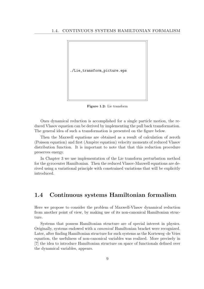
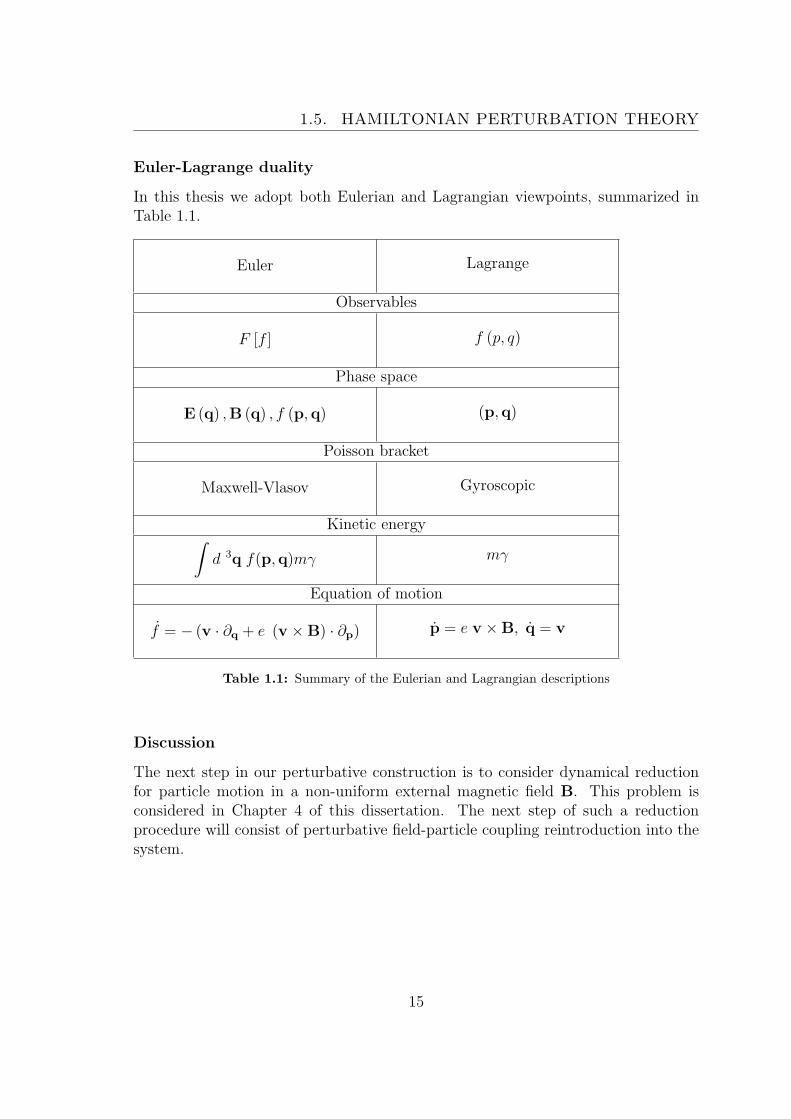
Euler-Lagrange duality
In this thesis we adopt both Eulerian and Lagrangian viewpoints, summarized inTable 1.1.
Euler Lagrange
Observables
F [f ] f (p, q)
Phase space
E (q) ,B (q) , f (p,q) (p,q)
Poisson bracket
Maxwell-Vlasov Gyroscopic
Kinetic energy∫d 3q f(p,q)mγ mγ
Equation of motion
f = − (v · ∂q + e (v ×B) · ∂p) p = e v ×B, q = v
Table 1.1: Summary of the Eulerian and Lagrangian descriptions
Discussion
The next step in our perturbative construction is to consider dynamical reductionfor particle motion in a non-uniform external magnetic field B. This problem isconsidered in Chapter 4 of this dissertation. The next step of such a reductionprocedure will consist of perturbative field-particle coupling reintroduction into thesystem.
15
CHAPTER 1. INTRODUCTION
Overview of the dissertation
The text of this dissertation is organized as follows.In Chapter 2 Hamiltonian control method is implemented in order to study
barrier formation in E × B drift model. Chapter 3 deals with investigation ofmomentum transport through derivation of the momentum conservation law forMaxwell-Vlasov equations.
Chapter 4 explores the fundamental geometrical problems related to the dynam-ical reduction of charged particle motion in an non-uniform magnetic field. Thiswork represents an important step in the construction of the alternative method fordynamical reduction of the Maxwell-Vlasov system.
16
Chapter 2
Barriers for the reduction oftransport due to the E ×B drift inmagnetized plasmas
Abstract.
We consider a 112degrees of freedom Hamiltonian dynamical sys-
tem, which models the chaotic dynamics of charged test-particles in aturbulent electric field, across the confining magnetic field in controlledthermonuclear fusion devices. The external electric field E = −∇V ismodeled by a phenomenological potential V and the magnetic field Bis considered uniform. It is shown that, by introducing a small addi-tive control term to the external electric field, it is possible to create atransport barrier for this dynamical system. The robustness of this con-trol method is also investigated. This theoretical study indicates thatalternative transport barriers can be triggered without requiring a con-trol action on the device scale as in present Internal Transport Barriers(ITB).
2.1 Introduction
It has long been recognized that the confinement properties of high performanceplasmas with magnetic confinement are governed by electromagnetic turbulence thatdevelops in microscales [11]. In that framework various scenarios are explored tolower the turbulent transport and therefore improve the overall performance of agiven device. The aim of such a research activity is two-fold.
First, an improvement with respect to the basic turbulent scenario, the so-calledL-mode (L for low) allows one to reduce the reactor size to achieve a given fusion
17
CHAPTER 2. BARRIERS FOR THE REDUCTION OF TRANSPORTDUE TO THE E ×B DRIFT IN MAGNETIZED PLASMAS
power and to improve the economical attractiveness of fusion energy production.This line of thought has been privileged for ITER that considers the H-mode (H forhigh) to achieve an energy amplification factor of 10 in its reference scenario [12].The H-mode scenario is based on a local reduction of the turbulent transport in anarrow regime in the vicinity of the outermoster confinement surface [13].
Second, in the so-called advanced tokamak scenarios, Internal Transport Barriersare considered [12]. These barriers are characterised by a local reduction of turbulenttransport with two important consequences, first an improvement of the core fusionperformance, second the generation of bootstrap current that provides a means togenerate the required plasma current in regime with strong gradients [14]. Theresearch on ITB then appears to be important in the quest of steady state operationof fusion reactors, an issue that also has important consequences for the operationof fusion reactors.
The H-mode appears as a spontaneous bifurcation of turbulent transport prop-erties in the edge plasma [13], the ITB scenarios are more difficult to generate in acontrolled fashion [15]. Indeed, they appear to be based on macroscopic modifica-tions of the confinement properties that are both difficult to drive and difficult tocontrol in order to optimise the performance.
In this paper, we propose an alternative approach to transport barriers based ona macroscopic control of the E × B turbulence. Our theoretical study is based ona localized hamiltonian control method that is well suited for E × B transport. Ina previous approach [16], a more global scheme was proposed with a reduction ofturbulent transport at each point of the phase space. In the present work, we derivean exact expression to govern a local control at a chosen position in phase space. Inprinciple, such an approach allows one to generate the required transport barriersin the regions of interest without enforcing large modification of the confinementproperties to achieve an ITB formation [15]. Although the application of such aprecise control scheme remains to be assessed, our approach shows that local controltransport barriers can be generated without requiring macroscopic changes of theplasma properties to trigger such barriers. The scope of the present work is thetheoretical demonstration of the control scheme and consequently the possibility ofgenerating transport barriers based on more specific control schemes than envisagedin present advanced scenarios.
In Section 2.2, we give the general description of our model and the physicalmotivations for our investigation. In Section 2.3, we explain the general methodof localized control for Hamiltonian systems and we estimate the size of the controlterm. Section 2.4 is devoted to the numerical investigations of the control term,and we discuss its robustness and its energy cost. The last section 2.5 is devoted toconclusions and discussion.
18
2.2. PHYSICAL MOTIVATIONS AND THE E ×B MODEL
2.2 Physical motivations and the E ×B model
2.2.1 Physical motivations
Fusion plasma are sophisticated systems that combine the intrinsic complexity ofneutral fluid turbulence and the self-consistent response of charged species, both elec-trons and ions, to magnetic fields. Regarding magnetic confinement in a tokamak, alarge external magnetic field and a first order induced magnetic field are organisedto generate the so-called magnetic equilibrium of nested toroidal magnetic surfaces[17]. On the latter, the plasma can be sustained close to a local thermodynamicalequilibrium. In order to analyse turbulent transport we consider plasma perturba-tions of this class of solutions with no evolution of the magnetic equilibrium, thusexcluding MHD instabilities. Such perturbations self-consistently generate electro-magnetic perturbations that feedback on the plasma evolution. Following presentexperimental evidence, we shall assume here that magnetic fluctuations have a neg-ligible impact on turbulent transport [18]. We will thus concentrate on electrostaticperturbations that correspond to the vanishing β limit, where β = p/(B2/2µ0)is the ratio of the plasma pressure p to the magnetic pressure. The appropriateframework for this turbulence is the Vlasov equation in the gyrokinetic approxi-mation associated with the Maxwell-Gauss equation that relates the electric fieldto the charge density. When considering the Ion Temperature Gradient instability[19] that appears to dominate the ion heat transport, one can further assume theelectron response to be adiabatic so that the plasma response is governed by thegyrokinetic Vlasov equation for the ion species.
Let us now consider the linear response of such a distribution function f , to a
given electrostatic perturbation, typically of the form Te ϕ e−iωt+ikr, (where f and
ϕ are Fourier amplitudes of distribution function and electric potential). To leadingorders one then finds that the plasma response exhibits a resonance:
f =
(ω + ω∗
ω − k|| v||− 1
)ϕfeq (2.1)
Here feq is the reference distribution function, locally Maxwellian with respect tov|| and ω
∗ is the diamagnetic frequency that contains the density and temperaturegradient that drive the ITG instability [19]. Te is the electronic temperature. Thissimplified plasma response to the electrostatic perturbation allows one to illustratethe turbulent control that is considered to trigger off transport barriers in presenttokamak experiments.
Let us examine the resonance ω − k|| v|| = 0 where k|| = (n −m/q)/R with Rbeing the major radius, q the safety factor that characterises the specific magneticequilibrium and m and n the wave numbers of the perturbation that yield the wavevectors of the perturbation in the two periodic directions of the tokamak equilibrium.When the turbulent frequency ω is small with respect to vth/(qR), (where vth =
19
CHAPTER 2. BARRIERS FOR THE REDUCTION OF TRANSPORTDUE TO THE E ×B DRIFT IN MAGNETIZED PLASMAS
√kBT/m is the thermal velocity), the resonance occurs for vanishing values of k||,
and as a consequence at given radial location due to the radial dependence of thesafety factor. The resonant effect is sketched on figure 2.1. In a quasilinear approach,
./Fig0.eps
Figure 2.1: Resonances for q = mn and q = m+1
n for two different widths, nar-row resonances empedding large scale turbulent transport and broad resonancesfavouring strong turbulent transport.
the response to the perturbations will lead to large scale turbulent transport whenthe width of the resonance δm is comparable to the distance between the resonances∆m,m+1 leading to an overlap criterion that is comparable to the well known Chirikovcriterion for chaotic transport σm = (δm + δm+1)/∆m,m+1 with σ > 1 leading toturbulent transport across the magnetic surfaces and σ < 1 localising the turbulenttransport to narrow radial regions in the vicinity of the resonant magnetic surfaces.
The present control schemes are two-fold. First, one can consider a large scaleradial electric field that governs a Doppler shift of the mode frequency ω. As suchthe Doppler shift ω − ωE has no effect. However a shear of the Doppler frequencyωE, ωE = ωE + δrω′
E will induce a shearing effect of the turbulent eddies and thuscontrol the radial extent of the mode δm, so that one can locally achieve σ < 1 inorder to drive a transport barrier.
Second, one can modify the magnetic equilibrium so that the distance betweenthe resonant surfaces is strongly increased in particular in a magnetic configura-tion with weak magnetic shear (dq/dr ≈ 0) so that ∆m,m+1 is strongly increased,∆m,m+1 ≫ δm, also leading to σ < 1.
Both control schemes for the generation of ITBs can be interpreted using thesituation sketched on figure 2.1. The initial situation with large scale radial transportacross the magnetic surfaces (so called L-mode) is indicated by the dashed lines andis governed by significant overlap between the resonances. The ITB control schemeaims at either reducing the width of the islands or increasing the distance betweenthe resonances yielding a situation sketeched by the plain line in figure 2.1 wherethe overlap is too small and a region with vanishing turbulent transport, the ITB,develops between the resonances.
Experimental strategies in advanced scenarios comprising Internal TransportBarriers are based on means to enforce these two control schemes. In both casesthey aim at modifying macroscopically the discharge conditions to fulfill locally the
20
2.2. PHYSICAL MOTIVATIONS AND THE E ×B MODEL
σ < 1 criterion. It thus appears interesting to devise a control scheme based on aless intrusive action that would allow one to modify the chaotic transport locallyby the choice of an appropriate electrostatic perturbation hence leading to a localtransport barrier.
2.2.2 The E ×B model
For fusion plasmas, the magnetic field B is slowly variable with respect to theinverse of the Larmor radius ρL i.e: ρL|∇ lnB| ≪ 1. This fact allows the separationof the motion of a charged test particle into a slow motion (parallel to the linesof the magnetic field) and a fast motion (Larmor rotation). This fast motion isnamed gyromotion, around some gyrocenter. In first approximation the averagingof the gyromotion over the gyroangle gives the approximate trajectory of the chargedparticle. This averaging is the guiding-center approximation.
In this approximation, the equations of motion of a charged test particle in thepresence of a strong uniform magnetic field B = Bz, (where z is the unit vector inthe z direction) and of an external time-dependent electric field E = −∇V1 are:
d
dT
X
Y
=cE×B
B2=
c
BE(X, Y, T )× z
=c
B
−∂Y V1(X,Y, T )∂XV1(X, Y, T )
(2.2)
where V1 is the electric potential. The spatial coordinates X and Y play the role ofcanonically-conjugate variables and the electric potential V1(X, Y, T ) is the Hamil-tonian for the problem. Now the problem is placed into a parallelepipedic box withdimensions L× ℓ× (2π/ω), where L and ℓ are some characteristic lengths and ω isa characteristic frequency of our problem, X is locally a radial coordinate and Y isa poloidal coordinate. A phenomenological model [20] is chosen for the potential:
V1(X,Y, T ) =N∑
n,m=1
V0 cosχn,m(n2 +m2)3/2
(2.3)
where V0 is some amplitude of the potential,
χn,m ≡2π
LnX +
2π
ℓmY + ϕn,m − ωT
ω is constant, for simplifying the numerical simulations and ϕn,m are some randomphases (uniformly distributed).
We introduce the dimensionless variables
(x, y, t) ≡ (2πX/L, 2πY/ℓ, ωT ) (2.4)
21
CHAPTER 2. BARRIERS FOR THE REDUCTION OF TRANSPORTDUE TO THE E ×B DRIFT IN MAGNETIZED PLASMAS
So the equations of motion (2.2) in these variables are:
d
dt
(xy
)=
(−∂yV (x, y, t)∂xV (x, y, t)
)(2.5)
where V = ε(V1/V0) is a dimensionless electric potential given by
V (x, y, t) = ε
N∑n,m=1
cos (nx+my + ϕn,m − t)(n2 +m2)3/2
(2.6)
Here
ε = 4π2(cV0/B)/(Lℓω) (2.7)
is the small dimensionless parameter of our problem. We perturb the model potential(2.6) in order to build a transport barrier. The system modeled by Eqs.(2.5) is a 11
2
degrees of freedom system with a chaotic dynamics [16, 20]. The poloidal sectionof our modeled tokamak is a Poincare section for this problem and the stroboscopicperiod will be chosen to be 2π, in term of the dimensionless variable t.
The particular choice (2.3) or (2.6) is not crucial and can be generalized. Gen-erally, ω can be chosen depending on n,m. This would make the numerical compu-tations more involved. In the following section, V is chosen completely arbitrary.
2.3 Localized control theory of hamiltonian sys-
tems
2.3.1 The control term
In this section we show how to construct a transport barrier for any electric po-tential V . The electric potential V (x, y, t) yields a non-autonomous Hamiltonian.We expand the two-dimensional phase space by including the canonically-conjugatevariables (w,τ),
H = H(x, τ ; y, w) = V (x, y, τ)− w (2.8)
The Hamiltonian of our system thus becomes autonomous. Here τ is a new variablewhose dynamics is trivial: τ = 1 i.e. τ = τ0 + t and w is the variable (momentum)canonically conjugate to τ . The Poisson bracket operator in the expanded phasespace for any U = U(x, τ ; y, w) is given by the expression:
U ≡ (∂xU)∂y − (∂yU)∂x + (∂τU)∂w − (∂wU)∂τ . (2.9)
Hence U is a linear (differential) operator acting on functions of (x, τ ; y, w). Wecall H0 = w the unperturbed Hamiltonian and V (x, y, τ) its perturbation. We now
22
2.3. LOCALIZED CONTROL THEORY OF HAMILTONIANSYSTEMS
implement a perturbation theory for H0. The operator of the Poisson bracket (4.6)for the Hamiltonian H is
H = (∂xV )∂y − (∂yV )∂x + ∂τ + (∂τV )∂w (2.10)
So the equations of motion in the expanded phase space are:
y = Hy = ∂xV (x, y, τ) (2.11)
x = Hx = − ∂yV (x, y, τ) (2.12)
w = Hw = ∂τV (x, y, τ) (2.13)
τ = Hτ = 1 (2.14)
We want to construct a small modification F of the potential V such that
H ≡ V (x, y, τ) + F (x, y, τ)− w ≡ V (x, y, τ)− w (2.15)
has a barrier at some chosen position x = x0. So the control term
F = V (x, y, τ)− V (x, y, τ) (2.16)
must be much smaller than the perturbation (e.g., quadratic in V ). One of thepossibilities is:
V ≡ V (x+ ∂yf(y, τ), y, τ) (2.17)
where
f(y, τ) ≡∫ τ
0
V (x0, y, t)dt
Indeed we have the following theorem:
Theorem 1 The Hamiltonian H has a trajectory x = x0 + ∂yf(y, τ) acting as abarrier in phase space.
ProofLet the Hamiltonian H ≡ exp(f)H be canonically related to H. (Indeed the
exponential of any Poisson bracket is a canonical transformation.) We show that Hhas a simple barrier at x = x0. We start with the computation of the bracket (4.6)for the function f . Since f = f(y, τ), the expression for this bracket contains onlytwo terms,
f ≡ −f ′∂x + f∂w (2.18)
wheref ′ ≡ ∂yf and f ≡ ∂τf (2.19)
which commute:[f ′∂x, f∂w] = 0 (2.20)
23
CHAPTER 2. BARRIERS FOR THE REDUCTION OF TRANSPORTDUE TO THE E ×B DRIFT IN MAGNETIZED PLASMAS
Now let us compute the coordinate transformation generated by exp(f):
exp(f) ≡ exp(−f ′∂x) exp(f∂w), (2.21)
where we used (2.20) to separate the two exponentials.Using the fact that exp(b∂x) is the translation operator of the variable x by the
quantity b: [exp(b∂x)W ](x) = W (x+ b), we obtain
H = efH ≡ efV (x, y, τ) − efw
= V (x− f ′, y, τ) −(w + f
)= V (x+ f ′ − f ′, y, τ)− V (x0, y, τ)− w= V (x, y, τ)− V (x0, y, τ)− w (2.22)
This Hamiltonian has a simple trajectory x = x0, w = w0, i.e. any initial datax = x0, y = y0, w = w0, τ = τ0 evolves under the flow of H into x = x0, y = yt, w =w0, τ = τ0 + t for some evolution yt that may be complicated, but not useful for ourproblem. Hamilton’s equations for x and w are now
x = Hx = ∂y [V (x0, y, τ)− V (x, y, τ)] (2.23)
w = Hw = ∂τ [V (x0, y, τ)− V (x, y, τ)] (2.24)
so that for x = x0, we find x = 0 = w. Then the union of all points (x, y, w, τ) atx = x0 w = w0:
B0 =∪y,τ,w0
x0yw0
τ
(2.25)
is a 3-dimensional surface T2 × R, (T ≡ R/2πZ) preserved by the flow of H in the4-dimensional phase space. If an initial condition starts on B0, its evolution underthe flow exp(tH) will remain on B0.
So we can say that B0 act as a barrier for the Hamiltonian H: the initial condi-tions starting inside B0 can’t evolve outside B0 and vice-versa.
To obtain the expression for a barrier B for H we deform the barrier for H viathe transformation exp(f). As
H = e−fH (2.26)
and exp(f) is a canonical transformation, we have
H = e−fH = e−fHef (2.27)
Now let us calculate the flow of H:
etH = et(e−fHef) = e−fetHef (2.28)
24
2.3. LOCALIZED CONTROL THEORY OF HAMILTONIANSYSTEMS
Indeed:
et(e−fHef) =
∞∑n=0
tn(e−fHef)n
n!(2.29)
For instance when n = 2:
t2(e−fHef)2 = t2e−fHefe−fHef
= t2e−fH2ef (2.30)
and so
etH =∞∑n=0
tne−fHnef
n!= e−fetHef (2.31)
As we have seen before:
ef
xywτ
=
x− f ′
y
w − fτ
and
etH
x0yw0
τ
=
x0ytw0
τ + t
(2.32)
Multiplying (2.28) on the right by e−f we obtain:
etHe−f = e−fetH
etHe−f
x0yw0
τ
= etH
x0 + f ′(y, τ)
y
w0 + f(y, τ)τ
(2.33)
and
e−fetH
x0yw0
τ
= e−f
x0ytw0
τ + t
=
x0 + f ′(yt, τ + t)
ytw0 + f(yt, τ + t)
τ + t
(2.34)
25
CHAPTER 2. BARRIERS FOR THE REDUCTION OF TRANSPORTDUE TO THE E ×B DRIFT IN MAGNETIZED PLASMAS
So the flow exp(tH) preserves the set
B =∪y,τ,w0
x0 + f ′(y, τ)
y
w0 + f(y, τ)τ
(2.35)
B is a 3 dimensional invariant surface, topologically equivalent to T2×R into the 4dimensional phase space. B separates the phase space into 2 parts, and is a barrierbetween its interior and its exterior. B is given by the deformation exp(f) of thesimple barrier B0.
The section of this barrier on the sub space (x, y, t) is topologically equivalentto a torus T2.
This method of control has been successfully applied to a real machine: a trav-eling wave tube to reduce its chaos [21].
2.3.2 Properties of the control term
In this Section, we estimate the size and the regularity of the control term (2.16).
Theorem 2 For the phenomenological potential (2.6) the control term (2.16) veri-fies:
∥F∥ 1N, 1N≤ ε2N2 e
3
4π(2.36)
if ε is small enough, i.e. if |ε| ≤√π
2Ne3/2where N is the number of modes in the sum
(2.6).
Proof The proof of this estimation is given in [22] and is based on rewriting
F = V (x+ f ′)− V (x) =
∫ 1
0
ds ∂xV (x+ sf ′, y, τ)f ′(y, τ)
= O(V 2) (2.37)
and then use Cauchy’s Theorem.
2.4 Numerical investigations for the control term
In this Section, we present the results of our numerical investigations for the controlterm F . The theoretical estimate presented in the previous section shows that itssize is quadratic in the perturbation. Figure 2.2 shows the contour plot of V (x, y, t)
26
2.4. NUMERICAL INVESTIGATIONS FOR THE CONTROL TERM
and V (x, y, t) (V = V +F ) at some fixed time t, for example t = π4. One can see that
the contours of both potentials are very similar. But the dynamics of the systemswith V and V are very different.
For all numerical simulations we choose the number of modes N = 25 in (2.6).In all plots the abscissa is x and the ordinate is y.
./Fig1.eps
Figure 2.2: Uncontrolled and controlled potential for ε = 0.6, t = π4 , x0 = 2.
2.4.1 Phase portrait for the exact control term
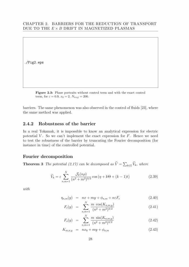
To explore the effectiveness of the barrier, we plot (in Fig. 2.3) the phase portraitsfor the original system (without control term) and for the system with the exactcontrol term F . We choose the same initial conditions. The time of integration isT = 2000, the number of trajectories: Ntraj = 200 (number of initial conditions, alltaken in the strip −1 − π ≤ x ≤ −π; 0 ≤ y ≤ 2π) and the parameter ε = 0.9. Wechoose the barrier at position x0 = 2. To get a Poincare section, we plot the poloidalsection when t ∈ 2πZ. Then we compare the number of trajectories passing throughthe barrier during this time of integration for each system. We eliminate the pointsafter the crossing. For the uncontrolled system 68% of the initial conditions crossthe barrier at x0 = 2 and for the controlled system only 1% of the trajectories escapefrom the zone of confinement. The theory announces the existence of an exact barrierfor the controlled system: these escaped trajectories (1%) are due to numerical errorsin the integration. One can observe that the barrier for the controlled system is astraight line. In fact this barrier moves, its expression depends on time:
x = x0 + f ′(y, t) (2.38)
But when t ∈ 2πZ its oscillation around x = x0 vanishes: f ′(y, 2kπ) =∫ 2kπ
0∂yV (x0, y, t)dt = 0. This is what we see on this phase portrait. In fact we
create 2 barriers at position x = x0, and x = x0− 2π (and also at x0+2nπ) becauseof the periodicity of the problem. We note that the mixing increases inside the two
27
CHAPTER 2. BARRIERS FOR THE REDUCTION OF TRANSPORTDUE TO THE E ×B DRIFT IN MAGNETIZED PLASMAS
./Fig2.eps
Figure 2.3: Phase portraits without control term and with the exact controlterm, for ε = 0.9, x0 = 2, Ntraj = 200.
barriers. The same phenomenon was also observed in the control of fluids [23], wherethe same method was applied.
2.4.2 Robustness of the barrier
In a real Tokamak, it is impossible to know an analytical expression for electricpotential V . So we can’t implement the exact expression for F . Hence we needto test the robustness of the barrier by truncating the Fourier decomposition (forinstance in time) of the controlled potential.
Fourier decomposition
Theorem 3 The potential (2.17) can be decomposed as V =∑
k∈Z Vk, where
Vk = εN∑
n,m=1
Jk(nρ)(n2 +m2)3/2
cos (η + kΘ+ (k − 1)t) (2.39)
with
ηn,m(y) = nx+my + ϕn,m + nεFc (2.40)
Fc(y) =N∑
n,m=1
m cos(Kn,m,y)
(n2 +m2)3/2(2.41)
Fs(y) =N∑
n,m=1
m sin(Kn,m,y)
(n2 +m2)3/2(2.42)
Km,n,y = nx0 +my + ϕn,m (2.43)
28
2.4. NUMERICAL INVESTIGATIONS FOR THE CONTROL TERM
and Jk is the Bessel’s function
Jk(nρ) =1
π
∫ π
0
cos (ku− nρ sinu) du (2.44)
Proof We rewrite explicitly the expression (2.17) for our phenomenological con-
trolled potential V (x, y, t):
V (x, y, t) =εN∑
n,m=1
cos(n(x+ f ′(y, t)) +my + ϕn,m − t
)(n2 +m2)3/2
(2.45)
with
f ′(y, t) = εN∑
n,m=1
m(cosKn,m,y − cos(Kn,m,y − t)
)(n2 +m2)3/2
(2.46)
With the definition (2.41) and (2.42) we have:
f ′(y, t) = ε(Fc(y) (1− cos t)− Fs(y) sin t) (2.47)
Let us introduceρ = ε(F 2
c + F 2s )
1/2 (2.48)
and Θ byρ sinΘ ≡ −εFc(y) ρ cosΘ ≡ −εFs(y) (2.49)
so that
V = εN∑
n,m=1
cos (η − t+ nρ sin(Θ + t))
(n2 +m2)3/2(2.50)
Using Bessel’s functions properties [24]
cos(ρ sinΘ) =∑k∈Z
Jk(ρ) cos kΘ (2.51)
sin(ρ sinΘ) =∑k∈Z
Jk(ρ) sin kΘ (2.52)
we get
cos (η − t+ nρ sin(Θ + t)) =∑k∈Z
Jk(nρ) cos (ξ) (2.53)
where ξ = η + kΘ + (k − 1)t, and we finally obtain (2.39). The theorem is proved.
During numerical simulations we truncate the controlled potential by keepingonly its first 3 temporal Fourier harmonics:
Vtr=εN∑
n,m=1
A0 + A1 cos t+B1 sin t+ A2 cos 2t+B2 sin 2t
(n2 +m2)3/2(2.54)
29
CHAPTER 2. BARRIERS FOR THE REDUCTION OF TRANSPORTDUE TO THE E ×B DRIFT IN MAGNETIZED PLASMAS
A0 = J0(nρ) cos(η +Θ)
A1 = J0(nρ) cos η + J2(nρ) cos(η + 2Θ)
B1 = J0(nρ) sin η − J2(nρ) sin(η + 2Θ)
A2 = J3(nρ) cos(η + 3Θ)− J1(nρ) cos(η −Θ)
B2 = −J3(nρ) sin(η + 3Θ)− J1(nρ) sin(η −Θ)
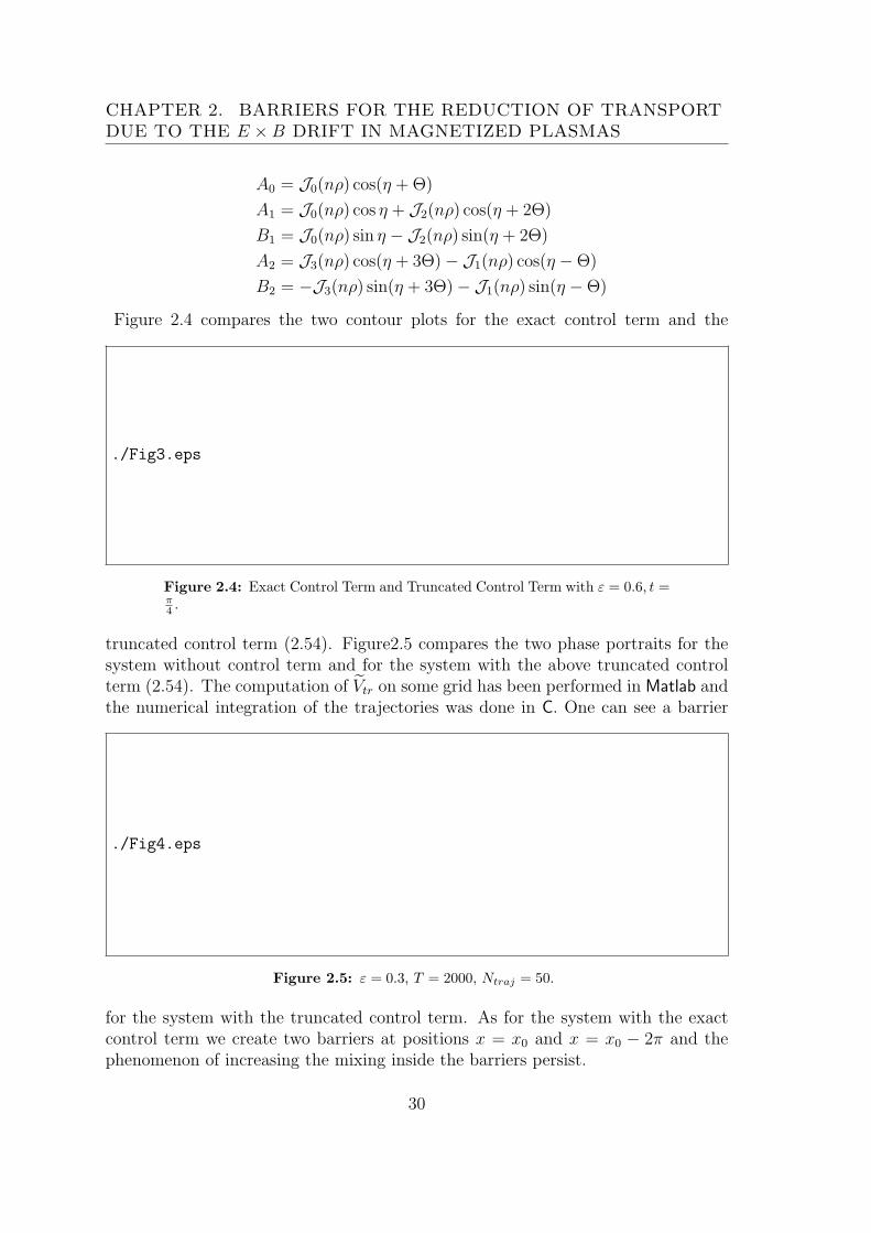
Figure 2.4 compares the two contour plots for the exact control term and the
./Fig3.eps
Figure 2.4: Exact Control Term and Truncated Control Term with ε = 0.6, t =π4 .
truncated control term (2.54). Figure2.5 compares the two phase portraits for thesystem without control term and for the system with the above truncated controlterm (2.54). The computation of Vtr on some grid has been performed in Matlab andthe numerical integration of the trajectories was done in C. One can see a barrier
./Fig4.eps
Figure 2.5: ε = 0.3, T = 2000, Ntraj = 50.
for the system with the truncated control term. As for the system with the exactcontrol term we create two barriers at positions x = x0 and x = x0 − 2π and thephenomenon of increasing the mixing inside the barriers persist.
30
2.4. NUMERICAL INVESTIGATIONS FOR THE CONTROL TERM
Table 2.1: Squared ratios of the amplitudes of the control term and the un-controlled electric potential ζex, ζtr; ratios of electric energy of the control termand the uncontrolled electric potential ηex, ηtr; for the system with exact andtruncated control term.
As we have seen before, the introduction of the control term into the system canreduce and even stop the diffusion of the particles through the barrier. Now weestimate the energy cost of the control term F and the truncated control termFtr ≡ Vtr − V .
Definition 1 The average of any functionW = W (x, y, τ) is defined by the formula:
< |W | >=∫ 2π
0
dx
∫ 2π
0
dy
∫ 2π
0
dt |W (x, y, t)| (2.55)
Now we calculate the ratio between the absolute value of the truncated control(electric potential) or the exact control and the uncontrolled electric potential:
ζex =< |F |2 > / < |V |2 >
and
ζtr =< |Ftr|2 > / < |V |2 >
We also compute the ratio between the energy of the control electric field and theenergy of the uncontrolled system in their exact and truncated version
ηex =< |∇F |2 > / < |∇V |2 >
and
ηtr =< |∇Ftr|2 > / < |∇V |2 >
for different values of ε. Results are shown in Table 2.1.
31
CHAPTER 2. BARRIERS FOR THE REDUCTION OF TRANSPORTDUE TO THE E ×B DRIFT IN MAGNETIZED PLASMAS
Table 2.2: Number of escaping particles without control term Nwithout, and forthe system with the exact control term Nexact and the truncated control termNtr.
Table 2.3: Difference ∆N of the number of particles passing through the barrierand difference of relative electric energy ∆η for the controlled and uncontrolledsystem.
One can see that the truncated control term needs a smaller energy than the exactcontrol term. In Table 2.2, we present the number of particles passing through thebarrier in function of ε, after the same integration time.
Let ∆N = Nwithout − Ntr be the difference between the number of particlespassing through the barrier for the system without control and with the truncatedcontrol and ∆η = ηex − ηtr the difference between the relative electric energy forthe system with the exact control term and the system with the truncated controlterm. In Table 2.3 we present ∆N and ∆η for differents values of ε.
For ε below 0.2 the non controlled system is rather regular, there is no particlesstream through the barrier, so we have no need to introduce the control electricfield. For ε between 0.3 and 0.9 the truncated control field is quite efficient, itallows to drop the chaotic transport through the barrier by a factor 8% to 24%with respect to the uncontrolled system and it requires less energy than the exactcontrol field. For ε greater than 1 the truncated control field is less efficient thanthe exact one, because the dynamics of the system is very chaotic. For examplewhen ε = 1.5, there are 72% of the particles crossing the barrier for the uncontrolledsystem and 54% for the system with the truncated control field. At the same timethe energetical cost of the truncated control field is above 70% of the exact one,which allows to stop the transport through the barrier. So for ε ≥ 1 we need to usethe exact control field rather than the truncated one.
32
2.5. DISCUSSION AND CONCLUSION
2.5 Discussion and Conclusion
In this article, we studied a possible improvement of the confinement properties ofa magnetized fusion plasma. A transport barrier conception method is proposedas an alternative to presently achieved barriers such as the H-mode and the ITBscenarios. One can note, that our method differs from an ITB construction. Indeed,in order to build-up a transport barrier, we do not require a hard modification ofthe system, such as a change in the q-profile. Rather, we propose a weak change ofthe system properties that allow a barrier to develop. However, our control schemerequires some knowledge and information relative to the turbulence at work, thesehaving weak or no impact on the ITB scenarios.
2.5.1 Main results
First of all we have proved that the local control theory gives the possibility toconstruct a transport barrier at any chosen position x = x0 for any electric potentialV (x, y, t). Indeed, the proof given in section 2.3 does not depend on the model for theelectric potential V . In Subsection 2.3.1, we give a rigorous estimate for the norm ofthe control term F , for some phenomenological model of the electric potential. Theintroduction of the exact control term into the system inhibits the particle transportthrough the barrier for any ε while the implementation of a truncated control termreduces the particle transport significantly for ε ∈ (0.3, 1.0).
2.5.2 Discussion, open questions
Comparison with the global control method
Let us now compare our approach with the global control method [16] which aimsat globally reducing the transport in every point of the phase space. Our approachaims at implementing a transport barrier. However, one also observes a globalmodification of the dynamics since the mixing properties seem to increase awayfrom the barriers.
Furthermore, in many cases, only the first few terms of the expansion of theglobal control term [16] can be computed explicitly. Here we have an explicit exactexpression for the local control term.
Effectiveness and properties of the control procedure
In subsection 2.2.2, we have introduced the dimensionless variables (2.4) and defineda dimensionless control parameter ε ≡ 4π2(cV0/B)/(Lℓω). In the simplifying casewhere l = L = 2π/k is the characteristic length of our problem, we have ε =ck2V0/(ωB). Let us consider a symmetric vortex, hence with characteristic scale1/k. Let us now consider the motion of a particle governed by such a vortex. The
33
CHAPTER 2. BARRIERS FOR THE REDUCTION OF TRANSPORTDUE TO THE E ×B DRIFT IN MAGNETIZED PLASMAS
order of magnitude of the drift velocity is therefore vE = kcV0/B and the associatedcharacteristic time τETT , τETT ≡ 1/(kvE), is the eddy turn over time. Let ω be thecharacteristic evolution frquency of the turbulent eddies, here of the electric field,then the Kubo number K is K = 1/ωτETT . This parameter is the dimensionlesscontrol parameter of this class of problems, and we remark that in our case K = ε.It is also important to remark that the parameter K also characterises the diffusionproperties of our system. Indeed, let δ be a step size of our particle in a randomwalk process and let τ be the associated characteristic time, the diffusion coefficientis then D = δ2/τ . Since one can relate the characteristic step and time by thevelocity, δ = vEτ , on also finds:
D =(vEτ)
2
τ=k2c2V 2
0
B2τ =
1
k2τ 2ETTτ =
K2
k2ω2τ (2.56)
We also introduce the reference diffusion coefficient D = k−2ω, so that:
D/D ≡ K2ωτ (2.57)
They are two asymptotic regimes for our system. The first one, is the regime ofweak turbulence, characterised by ωτETT ≫ 1 and therefore K ≪ 1. In this regime,the electric potential evolution is fast, the particle trajectories only follow the eddygeometry on distances much smaller than the eddy size. The steps δ are smalland the characteristic time τ of the random walk such that ωτ ≈ 1. The particlediffusion (2.57) is then such that:
D/D ≈ K2 for ωτETT ≫ 1 (2.58)
The second asymptotic regime is the regime of strong turbulence, with ωτETT ≪ 1and K ≫ 1. Particles then explore the eddies before decorrelation and the charac-teristic time of the random step is typically τ ≈ τETT and:
D/D ≈ K for ωτETT ≪ 1 (2.59)
The first regime corresponds to the weak turbulence limit with weak Kubo numberand particle diffusion and the second to strong turbulence and large Kubo numberand particle diffusion. The control method developed in this article does not dependon K ≡ ε. There is always a possibility to construct an exact transport barrier.However for the numerical simulations, we have remarked, that for small ε one canobserve a stable barrier without escaping particles, and for ε close or more than 1there is some leaking of particles across the barrier. The barrier is more difficultto enforce. Also when considering the truncated control term, one finds that thecontrol term is ineffective in the strong turbulence limit.
Let us now consider the implementation of our method to turbulent plasmaswhere the turbulent electric field is consistent with the particle transport. The the-oretical proof of an hamiltonian control concept is developped provided the system
34
2.5. DISCUSSION AND CONCLUSION
properties at work are completely known. For example the analytic expression forthe electric potential. This is impossible in a real system, since the measurementstake place on a finite spatio-temporal grid. This has motivated our investigation ofthe truncated control term by reducing the actually used information on the system.As pointed out previously, one finds that this approach is ineffective for strong tur-bulence. Another issue is the evolution of the turbulent electric field following theappearance of a transport barrier. This issue would deserve a specific analysis andvery likely updating the control term on a trasnport characteristic time scale. Analternative to such a process would be to use a retroactive Hamiltonian approach (aclassical field theory) [10] and to develop the control theory in that framework.
AcknowledgementsWe acknowledge very useful and encouraging discussions with A. Brizard, M.
Vlad and M. Pettini. This work supported by the European Communities underthe contract of Association between EURATOM and CEA was carried out within theframework of the European Fusion Development Agreement. The views and opinionsexpressed herein do not necessarily reflect those of the European Commission.
35
CHAPTER 2. BARRIERS FOR THE REDUCTION OF TRANSPORTDUE TO THE E ×B DRIFT IN MAGNETIZED PLASMAS
36
Chapter 3
Maxwell-Vlasov conservation law
3.1 Introduction and physical motivations
The Maxwell-Vlasov gyrokinetic approach represents a powerful tool for the inves-tigation of turbulent behavior of low-frequency strongly magnetized plasmas. It iswell known that one of the possible ways for investigating the properties of a physi-cal system is to derive its conservation laws. Noether’s theorem plays a fundamentalrole in theoretical physics by relating conservation laws and symmetries. For exam-ple, the energy conservation law is associated with symmetries under infinitesimaltime translation t→ t+ δt and momentum conservation law is associated with thesymmetries under infinitesimal spatial translations x→ x+ δx. Generally Noethermethod for fluids and plasmas can be presented for Euler-Lagrangian (E-L) andEuler-Poincare (E-P) variational principles which differ by their treatment of fieldsvariations. In fact, the essential difference between these variational principles is toconsider dynamical fields to be varied independently (E-L) or not. In what followswe deal with Euler-Poincare variational principle for Maxwell-Vlasov system. Weremark here that one of the serious advantages of Noether’s method for derivation ofgyrokinetic Maxwell-Vlasov system conservation laws is that this method permits usto obtain exactly conserved properties even for systems with asymptotically reduceddynamics.
The gyrokinetic energy conservation law was recently obtained in [25]. The goalof our study here is to derive an exact gyrokinetic Vlasov-Poisson momentum con-servation law. This investigation can have an important field of applications. Firstof all an exactly conserved quantity can be implemented as a numerical simulationsverification. In the other hand, interpreted like a momentum transport equation,momentum conservation law can also be used for investigation of intrinsic plasmarotation phenomena, which play an important role in fusion plasma stabilization.Further it can also be considered as a potential tool for plasma control by investi-gation of transport barrier creation.
In fact, transport barrier creation represents the results of one of the self-
37
CHAPTER 3. MAXWELL-VLASOV CONSERVATION LAW
consistent field-particle interaction. For example energy and momentum exchangebetween particles and fields in plasma. More precisely, energy exchange leads toplasma heating, and momentum exchange leads to current drive, so both phenom-ena can be considered as one of the sources for the transport barrier creation. Con-servation laws guarantee a proper exchange between particles and fields and thenpermits us to explore self-consistent mechanisms that govern plasma behavior.
3.2 Maxwell-Vlasov equations and variational
principles
Due to their large applicability Maxwell-Vlasov equations of ideal plasma dynamicshas a long history and was studied extensively. It was firstly used in their simplerform known as Poisson-Vlasov equations by Jeans [26]for investigation of structureformation on stellar and galactic scales and even before by Poincare [27] in his workon determination of stability conditions for stellar configurations. On the other handPoisson-Vlasov equation can be also applied in order to study self-consistent dynam-ics of electrostatic collisionless plasma whereas Maxwell-Vlasov equations permitsus to study self-consistent collisionless dynamics of plasma in electromagnetic fieldcase. In order to prepare the study of stability of plasma equilibrium, Low in 1956has presented his variational principle for Maxwell-Vlasov system. Low’s action isexpressed in mixture of Lagrangian particle variables and Eulerian fields variables.Since then a variety of variational formulations for Maxwell-Vlasov equations haveappeared. Particular attention was payed to the formulation of the particle partof the action. For example its mixed Eulerian-Lagrangian formulation was used inHamiltonian-Jacobi action presented in [28, 28–30] and [31]. A purely Eulerian for-mulation was proposed in [32, 33] through the introduction of two functions knownas Clebsch potentials introduced in [34, 35] and appropriate action principle withClebsch action. The leaf action variational principle introduced by Ye and Morrisonin [36] uses a single generating function as the dynamical variable for describingthe particle distribution and represents a link between Lagrangian and Eulerianrepresentations for actions. A more systematic derivation for a different Eulerianvariational principle was presented by Cendra et al in [37]. It is obtained by follow-ing the reduction procedure of Low variational principle, much as one does in thecorresponding derivation of non-canonical Poisson bracket in the Hamiltonian for-mulation for the Maxwell-Vlasov system. Similarly to ideal fluid Eulerian variationalprinciple, constrained variations on six dimensional phase space was introduced inthis work. Finally, a new Eulerian variational principle that uses constrained vari-ations on extended eight dimensional phase space was presented by A.J. Brizardin [38]. The transition from the six-dimensional phase space to the eight dimen-sional phase space permits us to express Vlasov distribution variation in terms ofcanonical Poisson bracket and a single scalar field δS which generate a virtual dis-
38
3.3. VARIATIONAL PRINCIPLE FOR PERTURBEDMAXWELL-VLASOV
placements on the extended phase space :Zα → Zα + δZα, α ∈ 1, . . . 8, whereδZα ≡ Zα, δS. In what follows we show how this variational principle can be ap-plied for derivation of conservation laws for perturbed Maxwell-Vlasov system andgyrokinetic Maxwell-Vlasov system in the case of electrostatic fluctuations.
3.3 Variational principle for perturbed Maxwell-
Vlasov
This section is dedicated to the derivation of momentum conservation law in the caseof the perturbed Maxwell-Vlasov system. In particular we consider that magneticfield is given by B = B0 + ϵB1 where B0 = ∇×A0 denotes the background time-independent equilibrium component, and B1 = ∇×A1 its fluctuation. At the sametime the electric field contains only a fluctuating part E1 = −∇Φ1 − c−1∂tA1.
In order to represent particle part of dynamics in extended eight dimensionalphase space, first of all we introduce an extended Hamiltonian H = H − w whereH is a Hamiltonian of a charged particle in an external perturbed electromagneticfield B1,E1:
H =1
2m(p− e
cA)2 + eϵ Φ1 (3.1)
where A ≡ A0 + ϵA1 Then we introduce extended Vlasov distribution function
F(Z) ≡ cδ(w −H)F (p,x) (3.2)
where F is the Vlasov distribution function on 6 dimensional phase space. Thisdefinition insures that the extended Hamiltonian H satisfies the physical constraintH = w. Here w is a variable that is canonically conjugate to t and the Poissonbracket is an extended canonical Poisson bracket:
F,Gext = ∇F ·∂G
∂p− ∂F
∂p· ∇G+
∂F
∂t· ∂G∂w− ∂F
∂w· ∂G∂t
(3.3)
Note that the dynamical variables in this approach are: electromagnetic fluctuatingfields B1, E1 and extended Vlasov distribution function F . Now we give an expres-sion for action functional corresponding to our system and then we use it order towrite corresponding Hamilton’s action principle δA ≡ 0:
A = −∫d8ZF(Z)H(Z; Φ1,A1)+
∫d4x
8π
(ϵ2|E1|2 − |B0 + ϵB1|2
)≡∫Ld4x (3.4)
Note that the extended phase space integration in the expression below is definedby d8Z ≡ c dtd3xd4p where d4p ≡ c−1d3pdw. In order to proceed with writing ofHamilton’s action principle
δA =
∫d4x δL = 0 (3.5)
we need first to obtain the Eulerian variation of Lagrangian density δL.
39
CHAPTER 3. MAXWELL-VLASOV CONSERVATION LAW
3.3.1 Eulerian variations
The Eulerian variation of the Lagrangian density given by expression (3.4) is ex-pressed as:
δL = −∫
(δFH + δHF) d4p+ ϵ
4π
(ϵ2 δE1 · E1 − ϵ δB1 ·B
)(3.6)
Here B0 is excluded as a variational field (since it is time independent). Eulerianelectromagnetic field variations are naturally related to the electromagnetic potentialvariations as follows
δE1 = −∇δΦ1 − c−1∂tδA1 (3.7)
δB1 = ∇× δA1 (3.8)
they satisfy the constraints given by two of Maxwell’s equations
∇× δE1 =1
c
∂δB1
∂t(3.9)
∇ · δB1 = 0 (3.10)
The Eulerian variation for the extended distribution function (3.2) is obtained byusing the fundamental relation between Eulerian (δF) and Lagrangian ∆F varia-tions:
δF ≡ ∆F − δZa ∂F∂Za
= −Za, Sext∂F∂Za
≡ S,Fext (3.11)
It preserves the Vlasov constraint∫Fd8Z = 0 under a virtual canonical transfor-
mation Za → Za + δZa in extended phase space (as a result of integration of anexact Poisson bracket over phase space). To obtain the expression (3.11) we usetwo facts. The first one is that the virtual canonical transformation is generatedby the extended scalar field S: δZa → Za + δZa. The second one is that the La-grangian variation of extended distribution function F is equal to zero. This is adirect consequence of the fact that the distribution function is constant along anytrajectory in the phase space (Liouville’s theorem). Finally the Eulerian variationof the extended Hamiltonian δH is given by:
δH = δΦ1δH
δΦ1
+ δA1 ·δH
δA1
(3.12)
Now our goal is to rewrite the expression for Lagrangian variation density (3.6) sothat the variation generators (S, δΦ1, δA1) appear explicitly
1. This will give us the
1You can find a detailed calculation that permits us the passage between the general expressionfor Maxwell-Vlasov Lagrangian density to the equations of motion and Noether’s terms in AppendixA
40
3.3. VARIATIONAL PRINCIPLE FOR PERTURBEDMAXWELL-VLASOV
possibility to derive the equations of motion and at the same time to obtain theNoether terms necessary for the derivation of conservation laws.
δL =
(∂Λ
∂t+∇ · Γ
)+ δΦ1
[ϵ2
4π∇ · E1 −
∫d4p
δH
δΦ1
F
](3.13)
+ δA1 ·[ϵ
4πc
(ϵ∂E1
∂t− c∇×B
)−∫d4p
δH
δA1
F
]−∫S F ,Hext d4p
where the Noether fields Λ and Γ are given by
Λ ≡∫d4p SF − ϵ2
4π cδA1 · E1 (3.14)
Γ ≡∫d4p S F x− ϵ2
4πδA1 ×B1 (3.15)
with x ≡ x, H representing the particle velocity. Note that here the Noetherspace-time divergence terms ∂Λ/∂t + ∇ · Γ do not contribute to the variationalprinciple.
Now we introduce this expression into Hamilton’s action principle (3.5). Hereeach term that is multiplied by the generators of the variations will give us corre-sponding equations of motion. All the other terms are expressed as divergence andexact time-derivative, and so do not influence the dynamics of the system. These arethe Noether terms, which contribute to the derivation of conservation laws. We re-mark that this expression is general and gives the possibility to obtain the equationsof motion and Noether terms for any system of Maxwell-Vlasov equations (reducedor not).
3.3.2 Perturbed Maxwell-Vlasov equations
In this section we deal with perturbed Maxwell-Vlasov system, so we use (3.1) inorder to obtain corresponding equations of motion. The functional derivatives δH
δΦ1
and δHδA1
are given by:
δH
δΦ1
= ϵe (3.16)
δH
δA1
= − ϵ
m
e
c
(p− e
c(A0 + ϵA1)
)≡ ϵ
e
cv (3.17)
So finally the perturbed Maxwell equations are given by the following expression:
ϵ∇ · E1 = 4πe
∫d4p F (3.18)
∇×B = ϵ1
c
∂E1
∂t+ 4πe
∫d4p F v
c(3.19)
41
CHAPTER 3. MAXWELL-VLASOV CONSERVATION LAW
Then the extended Vlasov equation is given by:
F ,Hext = 0 (3.20)
In order to obtain the Vlasov equation we perform the integration over the energycoordinate
∫dw of the extended Vlasov equation (see for details Appendix A.2.2).
∂F
∂t+ F,H = ∂F
∂t+∇F · ∂H
∂p−∇H · ∂F
∂p= 0 (3.21)
and then the perturbed Maxwell equations of motion become
ϵ∇ · E1 = 4πe
∫d3p F (3.22)
∇×B = ϵ1
c
∂E1
∂t+ 4πe
∫d3p F
v
c(3.23)
3.4 Momentum conservation law
In this section we use Noether method in order to derive exact momentum conserva-tion law for perturbed Maxwell-Vlasov system. The Noether’s theorem states thatfor each symmetry of the Lagrangian density L there corresponds a conservation law(and vice versa). When the Lagrangian is invariant under a time translation, a spacetranslation, or a spatial rotation, the conservation law involves energy, momentum,or angular momentum conservation respectively. The formal proof of this statementcan be found in [39].
After substituting the perturbed equations of motion (3.21,3.22,3.23) into theexpression for Eulerian variation of the Lagrangian density (3.14), we obtain Noetherequation:
δL =∂Λ
∂t+∇ · Γ (3.24)
Now the variations (S, δΦ1, δA1) are no longer consider arbitrary but are generatedby infinitesimal space-time translations correspondingly to the conservation law thatwe derive. Before we proceed with the derivation of the conservation laws, we notethat the Noether components (Λ,Γ) are defined up to the following transformations:
Λ ≡ Λ +∇ · η (3.25)
Γ ≡ Γ− ∂η
∂t+∇× σ (3.26)
where η and σ are arbitrary vector fields. These vector fields will be used in order toobtain conservation laws in gauge-independent form. Note that these transforma-tions are obtained naturally. In fact one can add and then sustain to the Noetherequation (3.24) the following quantity: ∇∂tη = ∂t∇η. Another vector field that wenote σ can be added to Γ component due to the fact that ∇ · (∇× σ) = 0 for anyvector field σ.
42
3.4. MOMENTUM CONSERVATION LAW
3.4.1 Constrained variations
Constrained variations for electromagnetic potentials
The variations of electromagnetic potentials generated by infinitesimal space-timetranslations can be expressed in terms of Lie-derivative £δx where δx represents aninfinitesimal translation in the four-dimensional phase space. In general theory theexpression for constrained variations of the Eulerian variational principle in termsof Lie-derivative appears when the equivalence between Lagrangian and Eulerianvariational principle is discussed. On the other hand, one can interpret this factonly by geometrical considerations, using the fact that the Lie -derivative can beviewed as a simple generalization of directional derivative. In this section we dealwith geometrical tools in order to obtain the expression for electromagnetic fieldconstrained variations.
We start with choice of the metric, here we deal with space-like or Minkowskitype of metric:
gµν = gµν =
−1 0 0 00 1 0 00 0 1 00 0 0 1
. (3.27)
We chose also the following definition of covariant and contravariant components:Aµ = (A0, Ai) and Aµ = gµνAν = (−A0, Ai). Infinitesimal space-time variationsare represented by the vector: δxµ = (−cδt, δxi) and covariant differentiation isgiven by: ∂µ = (−c−1∂t, ∂i) where ∂i ≡ ∂/∂xi. Then we can write an expression forone-form electromagnetic four potential.
A = Aµdxµ = −c A0 dt+A · dx (3.28)
Using the Cartan formula for Lie-derivative we have:
£δxA = iδx · dA+ d(iδx · A) (3.29)
where the inner product operator iδx acts as follows on one (A = Aµdxµ) and two
(∂µAνdxµ ∧ dxν) forms:
d(iδx · A) = dxν∂ν (Aµδxµ) = dxν∂ν
[−c A0 δt+ Aiδx
i]
(3.30)
iδx · dA = ∂µAν δxµ dxν − ∂µAν dxµ δxν ≡ δxµFµνdx
ν (3.31)
then£δxA = (δxµFµν + ∂ν(Aµδx
µ)) dxν ≡ −δAνdxν (3.32)
Then the variation of electromagnetic potential component:
δA0 = −δxiFi0 + c−1∂t(−A0cδt+ Ajδx
j)
(3.33)
δAi = cδtF0i − δxjFji − ∂i(−A0 c δt+ Ajδx
j)
(3.34)
43
CHAPTER 3. MAXWELL-VLASOV CONSERVATION LAW
By substituting the components of antisymmetric field tensor F0i = −∂iA0 −c−1∂tA and Fji = ∂jAi − ∂iAj we obtain:
δA0 = −δx · ∇A0 − δt ∂tA0 (3.35)
δA = −δx · ∇A− δt ∂tA (3.36)
We note here that Φ ≡ A0 and δΦ ≡ δA0, then
δΦ = −δxi ∂iΦ− δt ∂tΦ (3.37)
Another possibility to deal with covariant and contravariant vectors in this placeis to suppose that A0 = Φ and A0 = −Φ then the sign does not appear insidethe definition of covariant and contravariant components of vector potential Aµ =(A0, Ai) and A
µ = (A0, Ai). The infinitesimal space-time variations vector is δxµ =(δx0, δxi) with δx0 = cδt and ∂µ = (∂x0 , ∂xi) with ∂x0 = c−1∂t. Then A = Aµdx
µ =A0dx
0 +A · dx and using the Eq. (3.32) we obtain:
δA0 = −δxiFi0 − ∂0(A0δx
0 +A · dx)
(3.38)
δAi = −δx0F0i − δxjFji − ∂j(A0δx
0 +A · dx)
(3.39)
with F0i = ∂0Ai − ∂iA0 and Fij = ∂iAj − ∂jAi,
δA0 = −δxi∂iA0 − δt∂tA0 (3.40)
δAi = −δx · ∇A− δt∂tA (3.41)
Replacing now A0 ≡ −Φ we obtain (3.37)
Constrained variations for Lagrangian density
By analogy with constrained variations for electromagnetic potentials, using theCartan formula for Lie derivative, we can obtain the variation for Lagrangian density.In fact, let us consider four-form LΩ where Ω is the oriented space-time volumeelement, then
δL Ω ≡ −£δx (L Ω) (3.42)
Using the Cartan formula we obtain
£δx (L Ω) = d (iδx (L Ω)) + iδx (d (L Ω)) (3.43)
The second term in this expression is equal to zero because (d (d4x) ≡ 0), the firstterm can be rearranged as follows:
d (iδx (L Ω)) = (∂αL δxα) Ω (3.44)
here we use that:
iδx[dxα ∧ dxβ ∧ dxγ ∧ dxζ
]= δxα
(dxβ ∧ dxγ ∧ dxζ
)(3.45)
44
3.4. MOMENTUM CONSERVATION LAW
andd (L iδxΩ) = ∂αLδxα
(dxα ∧ dxβ ∧ dxγ ∧ dxζ
)≡ (∂αL δxα) Ω (3.46)
By substituting the formula (3.44) into the expression (3.42) we obtain:
δL = −∂µ (δxµ L) (3.47)
Due to the fact that in our approach we decompose the initial magnetic field intoits dynamical part B1 and its background part B0 we should take it into accountwhen defining the Eulerian variation of Lagrangian density. In order to do that, wecorrect the expression for variation δL by subtracting from ∂µL the derivative of theLagrangian density with respect to the space-time variables while all the dynamicalfields are held constant. Then only the background fields contribute. We indicatesuch a derivative by ∂′µL. So finally
δL = −δxi (∂iL − ∂′iL) + δt (∂tL − ∂′tL) (3.48)
3.4.2 Noether method
In order to obtain the momentum conservation law for the perturbed Maxwell-Vlasov system, we use the Noether equation (3.24) and consider infinitesimal spacetranslations x→ x+ δx generated by:
where the expression for canonical particle momentum p∗ will be discussed be-low. The expression for variations of electromagnetic fields δΦ1, δA1, δL are ob-tained from the general theory as the spatial component of the Lie derivativeδA = δAµdx
µ ≡ −£δxA and δL Ω = −£δx (L Ω). Here the notation ∇′L inthe expression for δL denotes the explicit spatial gradient of the Lagrangian den-sity L with dynamical fields E1,B1, F held constant. Since we consider the case ofspatially uniform background magnetic field B0, we have
∇′L ≡ ∇B0 ·∂L∂B0
= −∇B0 ·(B
4π+
∫F∂H
∂B0
d3p
)(3.50)
where the first term denotes the contribution from the Maxwell part LM ≡ (ϵ2|E1|2−|B|2)/8π of the Lagrangian density while the second term involves the magnetizationcontribution associated with the background magnetic field [40]. Then the secondterm is formally equal to zero while we still work in canonical variables. In fact,in our case the particle Hamiltonian (3.1) is expressed in terms of electromagneticpotential A = A0 + ϵA1, and not magnetic field B0 = ∇×A0.
45
CHAPTER 3. MAXWELL-VLASOV CONSERVATION LAW
Primitive momentum conservation law
By inserting the variations (3.49) into the Noether equation (3.24), we obtain theprimitive momentum conservation law
− (∇L−∇′L) = ∂
∂t
[∫F (p∗ · δx) d4p−
ϵ2
4π c(δx×B1 −∇δχ1) · E1
]+ ∇ ·
[∫F (p∗ · δx) xd4p−
ϵ2
4π
(δx · E1 +
1
c
∂δχ1
∂t
)E1
− ϵ
4π(δx×B1 −∇δχ1)×B
](3.51)
where we have introduced a gauge-dependent field δχ1 ≡ A1 · δx and rewrite thevariations (3.49) as displayed. Consequently to that this primitive form of the mo-mentum conservation law is not gauge invariant.
Gauge-independent momentum conservation law
In order to remove the gauge-dependent term in expression (3.51), we use the trans-formations (3.26), with η ≡ (ϵ2/4π c)(A1 · δx)E1 and σ ≡ (ϵ/4π)(A1 · δx) B (thedetails of this calculation are given in the Appendix). Finally the gauge-independentmomentum conservation law is
∂P
∂t+∇ ·Π = ∇B0 ·
∂L∂B0
(3.52)
According to the Noether theorem, the component of the gyrokinetic momentumin the direction of the background magnetic field B0 field spatial symmetry is con-served.
Here the momentum density, after integrating over energy variable∫dw, is
P =
∫F(p∗ − ϵ
e
cA1
)d3p+
ϵ2
4πcE1 ×B1 (3.53)
and the canonical momentum-stress tensor is
Π =
[ϵ2
8π
(|E1|2 + |B1|2
)− |B0|2
8π
]I− 1
4π
(ϵ2E1E1 + ϵB1B
)+
∫F[x p∗ − ϵ
e
c(v A1)
]d3p (3.54)
Note that we take into account the Vlasov condition FH ≡ 0 in extended phasespace when evaluating the derivative ∇L, so only the Maxwell part of Lagrangiandensity will give the contribution in Π.
46
3.4. MOMENTUM CONSERVATION LAW
3.4.3 Proof of Momentum conservation
In this section we give an explicit proof of the momentum conservation law (3.52).We will see that the momentum conservation yields the dynamics of the system. Westart by taking partial time derivative of the perturbed momentum density (3.53):
∂P
∂t=
∫ [∂F
∂t
(p∗ − ϵ
e
cA1
)+ F
∂
∂t
(p∗ − ϵ
e
cA1
)]d3p
+ϵ2
4π c
(∂E1
∂t×B1 + E1 ×
∂B1
∂t
)(3.55)
By substituting into the expression below the Maxwell-Vlasov equations (3.22 , 3.23)and the Vlasov equation in the phase-space divergence form:
∂F
∂t+∇ · (F x)− ∂
∂p· (F p) = 0 (3.56)
we have:
∂P
∂t= −∇ ·
[∫F x
(p∗ − ϵ
e
cA1
)d3p+
ϵ2
8π
(|E1|2 + |B1|2
)− 1
4π
(ϵ B1B+ ϵ2E1E1
)]− ϵ
4π∇B0 ·B1 +
∫F
[d
dt
(p∗ − ϵ
e
cA1
)− ϵ e
(E1 +
v
c×B1
)]d3p (3.57)
whered
dt
(p∗ − ϵ
e
cA1
)≡ ∂
∂t
(p∗ − ϵ
e
cA1
)+ (p∗ − ϵ
e
cA1
), H (3.58)
The detailed calculation that permits us the transition between the Eq.(3.55) to theEq. (3.57) is given in the appendix B. Now we add ∇·Π to the result of the explicittime differentiation of the perturbed momentum density ∂P/∂t, where Π is definedby the Eq. (3.54). So the momentum conservation law (3.52) becomes:
0 ≡ ∂P
∂t+∇ ·Π−∇B0 ·
∂L∂B0
(3.59)
=
∫F
[d
dt
(p∗ − ϵ
e
cA1
)− ϵ e
(E1 +
v
c×B1
)]d3p
Therefore, the last equation yields the perturbed canonical momentum equation:
d
dt
(p∗ − ϵ
e
cA1
)≡ ϵ e
(E1 +
v
c×B1
)(3.60)
The equation (3.60) can be used to define the perturbed canonical momentum p∗that intervenes when defining the generating function of spatial translations (3.49).We remark that we can replace the momentum conservation law for the perturbedMaxwell-Vlasov system (3.52) by the equation for perturbed canonical momentumin the particle phase space (3.60). This connection is analogous to the standard con-nection between the momentum conservation law and the equation for the particlecanonical momentum in the case of the non-perturbed Maxwell-Vlasov system.
47
CHAPTER 3. MAXWELL-VLASOV CONSERVATION LAW
3.4.4 Particle canonical momentum
In previous section we have obtained the equation for the perturbed canonical mo-mentum p∗. We now discuss its properties by comparing with the case of theunperturbed Maxwell-Vlasov system.
In general theory [38] for the full Maxwell-Vlasov system when magnetic fieldis not divided into its equilibrium (non-dynamical part) and perturbed (dynamical)part, the generating function S for the derivation of the momentum conservationlaw is given by the particle canonical momentum p ≡ mv + e
cA.
Let see now what changes for the perturbed Maxwell-Vlasov system, when theelectromagnetic fields E ≡ ϵE1 = −Φ1 − c−1∂tA1 and B ≡ B0 + ϵB1 = ∇ ×(A0 + ϵA1) are expressed in terms of background fields (0,B0) and perturbationfields (E1,B1). In this case the corresponding particle canonical momentum shouldbe expressed as p ≡ mv + e
cA0 + ϵ e
cA1 and the corresponding equation of motion
that can be directly derived from the Hamiltonian (3.1) is (see for details C):
d
dt
(p− e
cA0 − ϵ
e
cA1
)= e
(ϵ E1 +
v
c× (B0 + ϵ B1)
)(3.61)
Let now compare this equation to the equation (3.60) for the perturbed canonicalmomentum p∗. First we can remark that the magnetic part of the Lorentz forcein r.h.s of the equation (3.60) does not contain the contribution coming from theequilibrium magnetic field B0, there is only the contribution coming from the dy-namical electromagnetic fields B1 and E1. We remark that such an equation can bederived from the Hamiltonian (3.1) after performing on it the gauge transformationA→ A′ = A−∇χ where the gauge field is chosen such that ∇χ ≡ A0
H =1
2m
(p− ϵe
cA1
)2+ ϵ e Φ1 (3.62)
Then in order to be coherent, p∗ should be defined as follows
p∗ = mv + ϵe
cA1 (3.63)
It represents a mixed-canonical momentum (i.e., it is a kinetic momentum in theabsence of the magnetic field perturbation generated by the vector field A1). Wecan see that the generating function S for the perturbed Maxwell-Vlasov systemcontains only the dynamical part of the vector potential.
Now we use the expression for the mixed-canonical momentum p∗ (3.63) in orderto simplify the expressions for the momentum density (3.53) and the momentumcanonical tensor (3.54). Finally we obtain the expressions for the momentum density
48
3.5. GYROKINETIC VARIATIONAL PRINCIPLE
and the momentum stress tensor with symmetrized Vlasov part:
P =
∫F v d3p+
ϵ2
4πcE1 ×B1 (3.64)
Π =
[ϵ2
8π
(|E1|2 + |B1|2
)− |B0|2
8π
]I− 1
4π
(ϵ2E1E1 + ϵB1B
)+
∫F mvv d3p (3.65)
3.4.5 Momentum conservation law in background separatedform
In this section we show how the momentum conservation law can be used in orderto study the momentum exchange between the background field and plasma. Fordoing this we rewrite the momentum conservation law in its background separatedform. We define
P ≡ P =
∫F
v
cd3p (3.66)
Π = Π+|B0|2
8πI+
ϵ
4πB1 ·B0 =
ϵ2
8π
[(|E1|2 + |B1|2
)]I− 1
4π
(ϵ2E1E1 + ϵB1B1
)+
∫F mvv d3p (3.67)
Then the momentum conservation law (3.52) became:
∂P
∂t+∇ ·Π =
1
4πJ0 ×B1 (3.68)
where we make appear the background component of current J0 ≡ (∇×B0), weuse that ∇· (B1 B0)−∇B0 ·B1 = (∇×B0)×B1. Let us now consider the equation(3.68), its l.h.s. contains purely plasma contributions into the momentum densityP and the momentum stress tensor Π, the r.h.s. contains the coupling betweenthe background magnetic field B0, represented by background current J0, and theplasma magnetic field B1. So we can say that momentum conservation law describesexchange between the background fields and plasma.
3.5 Gyrokinetic variational principle
In sections 3.3 and 3.4 we have considered derivation of momentum conservation lawfor perturbed Maxwell-Vlasov system. In this section we will deal with derivation
49
CHAPTER 3. MAXWELL-VLASOV CONSERVATION LAW
of momentum conservation law in the case of reduced (by using the Lie-transformmethod [41]) Maxwell-Vlasov system. Note that differently from the perturbedMaxwell-Vlasov system case, here we consider only the electrostatic fluctuations withdynamical electric field E1 = −∇Φ1 and the non-dynamical background magneticfield B0 = ∇×A0. The case of the electromagnetic fluctuations represents a partof the future work.
Previously, several works dealt with variational formulation of reduced Maxwell-Vlasov system. For example Sugama in [42] has presented Lagrangian variationalprinciple, in which an action functional for gyrocenter particles was derived fromthe Low Lagrangian formalism. Here we still use the Eulerian variational principleproposed by A.J. Brizard in [38] and then adapted by him in [43] for the case of thereduced Maxwell-Vlasov system.
Here we generally follow the same schema for momentum conservation law deriva-tion that in the case of the perturbed Maxwell-Vlasov system.
Gyrokinetic action functional for electrostatic perturbation
In order to prepare the introduction of gyrokinetic electrostatic Maxwell-Vlasovaction functional, we first present extended reduced (gyrocenter) Hamiltonian Hgy
and Vlasov distribution function Fgy. Accordingly to the Lie-transform phase spacemethod for gyrokinetic dynamical reduction [44], the gyrocenter Hamiltonian isgiven by
Hgy
(X, p ||, µ, t,Φ1
)= Hgc
(X, p ||, µ
)+ ⟨ϵ e Φ1 gc⟩ −
ϵ2
2e ⟨£gyΦ1 gc⟩ (3.69)
where ⟨. . . ⟩ denotes the gyroangle-averaging operation, the unperturbed gyrocenterHamiltonian is defined as the guiding-center Hamiltonian Hgc ≡ µB0 + p2||/2m, theeffective first-order guiding-center potential in electrostatic turbulence case is
Φ1gc ≡= T−1gc Φ1 (3.70)
where T−1gc denotes push-forward gyrocenter operator. The second order pondero-
motive potential in Eq. (3.69) is expressed in terms of the gyrocenter Lie-derivative£gy [25], which is defined for a general function G in electrostatic turbulence caseas
£gyG ≡e
ΩΨ1gc, Ggc (3.71)
where . , .gc represents the guiding-center Poisson bracket [45] and Ψ1gc is definedfrom the following equation:
∂θΨ1 ≡ Φ1gc = e (Φ1gc − ⟨Φ1gc⟩) (3.72)
Ω = eB0/mc denotes the Larmor frequency. We remark that while the gyroangle-averaged potential ⟨ϕ1gc⟩ contributes to the linear (first order) perturbed gyrocenter
50
3.5. GYROKINETIC VARIATIONAL PRINCIPLE
Hamiltonian dynamics, the gyroangle-dependent potential Φ1gc contributes to the(second-order) gyrocenter ponderomotive Hamiltonian in Eq.(3.69). The extendedgyrocenter Hamiltonian
Hgy
(X, p ||, µ, t, w; Φ1
)≡ Hgy
(X, p ||, µ, t; Φ1
)− w (3.73)
is expressed in terms of the time-dependent gyrocenter Hamiltonian given by Eq.(3.69) and the gyrocenter energy coordinate w. The extended Vlasov distributionfunction
Fgy(Z) ≡ F (X, p ||, µ, t) c δ(w −Hgy) (3.74)
ensures that the gyrocenter Hamiltonian dynamics satisfies the physical constraintHgy ≡ 0. Now we have all the elements to give the expression for the electro-static gyrokinetic action functional Agy and to the corresponding Hamilton’s actionprinciple δAgy = 0.
Agy = −∫d8Z Fgy (Z) Hgy (Z; Φ1) +
∫d4x
8π
(|E1|2 − |B0|2
)≡∫Lgy d4x (3.75)
Note that now the integration is realized over the extended reduced phase spaced8Z ≡ dt d3X d4p, where d4p ≡ c−1dw d3p and d3p = 2π m B∗
|| dp || dµ. Here2π m B∗
|| represents the Jacobian of the guiding-center transformation.
3.5.1 Eulerian variations
The general expression for Eulerian variation of Lagrangian density in the case ofgyrokinetic Maxwell-Vlasov system Lgy is given by:
δLgy =ϵ
4π
[(δE1 · E1)−
∫δFgy Hgy + ϵ
(δΦ1
δHgy
δΦ1
)Fgy]
(3.76)
where B0 is a non-dynamical field and the constrained Eulerian variation for electricfield δE1 = −∇Φ1 preserves the constraint c∇ × δE1 = 0. The Eulerian variationfor the extended gyrocenter Vlasov distribution is
δFgy ≡ Sgy,Fgyϵ (3.77)
where ., .ϵ denotes the extended guiding-center Poisson bracket. Similarly to pre-vious case this Eulerian variation preserves the Vlasov constraint
∫δFgyd8Z = 0
under a virtual canonical transformation Z → Z + δZ in extended phase space.Now the virtual canonical transformation is generated by the extended scalar fieldSgy: δZα ≡ Zα, Sgyϵ
51
CHAPTER 3. MAXWELL-VLASOV CONSERVATION LAW
Gyrocenter Hamiltonian functional derivative
In this subsection we give some details about evaluation of functional derivativeδHgy/δΦ(x). Before starting this calculation we have to make some remarks.
Due to the gyrokinetic dynamical reduction one have to pay attention to thefact that the electromagnetic fields Φ1 = Φ1(x),A0 = A0(x) and the particle (gy-rocenters) X are now evaluated at different spatial positions. The fields are stillevaluated at the full particle position x while the positions of the gyrocenters areX ≡ x − ρ0 where the difference between them is ρ0 which denotes the Larmorradius. To give the link between the electric field evaluated in the position x andthe gyrocenter electric field evaluated into the reduced (gyrocenter) position, weintroduce the guiding-center delta function δ3gc ≡ δ3 (X+ ρ0 − x). It indicates thatthe gyrocenter contribution at a fixed point x only comes from gyrocenters locatedon the ring X = x− ρ0. Then
Φ1gc =
∫d3x δ3gc Φ1(x) (3.78)
The variation of the gyrocenter Hamiltonian (3.69) is given by:
δHgy = ϵ e⟨δΦ1gc⟩ −ϵ2 e2
2Ω⟨δΨ1gc, Φ1gcgc + Ψ1gc, δΦ1gcgc⟩ (3.79)
Accordingly to the Eq.(3.78), functional derivative of the first order gyrocenterHamiltonian is
⟨δΦ1gc⟩δΦ1(x)
= δ3gc (3.80)
In order to evaluate functional derivative of the second order correction to the gy-rocenter Hamiltonian, we integrate it by parts with Φ1gc = ∂θΨ1gc
⟨δΨ1gc, Φ1gcgc⟩ = ⟨δΨ1gc,∂Ψ1gc
∂θgc⟩ = −⟨
∂δΨ1gc
∂θ, Ψ1gcgc⟩
= −⟨δΦ1gc, Ψ1gcgc⟩ = ⟨Ψ1gc, δΦ1gcgc⟩ (3.81)
ThenδHgy
δΦ1(x)= ϵ e⟨δ3gc⟩ −
ϵ2 e2
Ω⟨Ψ1gc, δ
3gcgc⟩ ≡ ⟨T−1
gc δ3gc⟩ (3.82)
Here we make appear the push-forward gyrocenter operator T−1gc ≡ 1− ϵ£gy (up to
the first order).Following the schema presented for perturbed Maxwell-Vlasov system we rewrite
the expression (3.76) for Eulerian variations of Lgy so that the variations generators(Sgy, δΦ1) appears explicitly:
δLgy =
(∂Λ
∂t+∇ · Γ
)−∫
SgyFgy,Hgyϵ d4p
+ δΦ1
[ϵ2
4π∇ · E1 − ϵ e
∫Fgy⟨T−1
gc δ3gc⟩d4p d3X
](3.83)
52
3.6. GYROKINETIC MOMENTUM CONSERVATION LAW
here we have used Eq.(3.82) and Eq.(3.77). The Noether fields Λ and Γ that doesnot contribute to the variational principle
Λ ≡∫
SgyFgyd4p (3.84)
Γ ≡∫
Sgy Fgy X d4p− ϵ2
4πδΦ1 E1 (3.85)
with X ≡ X, Hgygc representing the gyroangle-independent gyrocenter velocity.
3.5.2 Gyrokinetic Maxwell-Vlasov equations
After substituting the variation (3.83) into the variational principle∫δLgyd4x =
0 for arbitrary variation generators (Sgy, δΦ1), we obtain the gyrokinetic Vlasovequation
Fgy,Hgyϵ = 0 (3.86)
and the gyrokinetic Poisson equation:
ϵ ∇ · E1 = 4π e
∫Fgy⟨T−1
gc δ3gc⟩d 4p d 3X (3.87)
Performing the integration over the energy coordinate (∫dw) on the extended gy-
rokinetic Vlasov equation (3.86) we obtain the gyrokinetic Vlasov equation (see fordetails Appendix A.2.2).
∂F
∂t+ F,Hgygc ≡
∂F
∂t+ X · ∇F + p ||
∂F
∂p ||= 0 (3.88)
and the gyrokinetic Poisson equation
ϵ ∇ · E1 = 4π e
∫F ⟨T−1
gc δ3gc⟩d 3p d 3X (3.89)
3.6 Gyrokinetic momentum conservation law
Following the procedure for deriving the momentum conservation law that was es-tablished for the perturbed Maxwell-Vlasov system case, we now substitute thegyrokinetic Vlasov-Poisson equations (3.88) and (3.89) into the variational equation(3.83), we obtain the corresponding Noether equation
δLgy =∂Λ
∂t+∇ · Γ (3.90)
where Λ and Γ are defined up to the transformation (3.26).
53
CHAPTER 3. MAXWELL-VLASOV CONSERVATION LAW
3.6.1 Noether Method
Comparing to the expressions (3.49) for the variations generated by infinitesimalspace translations x→ x+ δx in the case of the full perturbed Maxwell-Vlasov sys-tem, the variations (Sgy,Φ1) for the gyrokinetic electrostatic Vlasov-Maxwell systemare now given by:
Sgy = pgy · δx (3.91)
δΦ1 = −δx · ∇Φ1 ≡ δx · E1 (3.92)
δLgy = −δx · (∇Lgy −∇′Lgy) (3.93)
where Sgy is the gyrocenter generating scalar field for the virtual spatial translationδx contains gyrocenter canonical momentum pgy its expression will be discussedbelow. The expressions for electric field variation and Lagrangian density variationare obtained following the same procedure that was presented in Section 3.4.1. Notethat comparing to the Eq. (3.50) for the derivative of the Lagrangian density withrespect to the background magnetic field B0 we should replace L by Lgy and H byHgy:
∇′Lgy ≡ ∇B0 ·∂Lgy∂B0
= −∇B0 ·(B0
4π+
∫F∂Hgy
∂B0
d 3p
)(3.94)
We note also that in the absence of the perturbed magnetic field B1 the momentumconservation law that we derive is directly gauge independent:
−δx · (∇Lgy −∇′Lgy) =∂
∂t
[∫Fgy (⟨pgy⟩ · δx) d4p
](3.95)
+ ∇ ·[∫Fgy (⟨pgy⟩ · δx) Xgy d
4p− ϵ2
4πδx · E1E1
]Note that while deriving this momentum conservation law we have used only thegyroaveraged part of the generating function Sgy = ⟨pgy⟩. In fact it is necessaryin order to be coherent with dynamics generated by the gyrocenter gyroangle-independent Hamiltonian (3.69). For example the gyrokinetic Poisson equation(3.89) is driven only by the gyroaveraged part of the gyrokinetic charge densityρgk ≡
∫F ⟨T−1
gy δ3gc⟩d 3p. In what concerns the gyrokinetic Vlasov equation (3.88),
it is obtained by assuming supplementary that ∂θF = 0 (see appendix A.2.2).Then we rewrite the expression (3.94) as
∂Pgy
∂t+∇ ·Πgy = ∇B0 ·
∂Lgy∂B0
≡ ∂′Lgy (3.96)
Then by performing the integration over the energy coordinate∫dw, the gyrokinetic
momentum density is
Pgy =
∫F ⟨pgy⟩ d3p (3.97)
54
3.6. GYROKINETIC MOMENTUM CONSERVATION LAW
and the gyrokinetic momentum stress tensor is
Πgy =1
8π
(ϵ2|E1|2 − |B0|2
)I− ϵ2
4πE1E1 +
∫F Xgy ⟨pgy⟩ d3p (3.98)
where Xgy ≡ X, Hgygc
3.6.2 Proof of Gyrokinetic Momentum conservation
As in previous case we give an explicit proof of the gyrokinetic momentum con-servation law (3.96). We begin with the partial time derivative of the gyrokineticmomentum density (3.97):
∂Pgy
∂t=
∫ [∂F
∂t⟨pgy⟩+ F
∂⟨pgy⟩∂t
]d 3p (3.99)
By substituting corresponding gyrokinetic Vlasov equation in its phase-space diver-gence form (see for details appendix A.2.2)
F,Hgygc =1
B∗||∇ ·(B∗
|| X F)+
1
B∗||
∂
∂p ||
(B∗
|| p || F)
(3.100)
after integration by parts we obtain
∂Pgy
∂t=
∫Fdgy ⟨pgy⟩
dtd 3p−∇ ·
[∫F Xgy ⟨pgy⟩
]d 3p (3.101)
wheredgy ⟨pgy⟩
dt≡ ∂⟨pgy⟩
∂t+ ⟨pgy⟩, Hgygc (3.102)
Due to the fact that we have taken only the gyroaveraged part of the generatingfunction Sgy in order to derive the gyrokinetic momentum conservation law and only⟨pgy⟩ intervene into our calculations, we have:
B∗||⟨pgy⟩, Hgygc = ∇ ·
(B∗
|| ⟨pgy⟩ Xgy
)+
∂
∂p ||
(B∗
|| ⟨pgy⟩ ˙p ||)
(3.103)
Now we use the gyrokinetic Poisson equation (3.89) and the electrostatic constraint∇ × E1 = 0 in order to perform the electrostatic Maxwell part of the gyrokineticmomentum stress divergence ∇ ·Πgy
ϵ2
4π∇ ·(1
2|E1|2 − E1E1
)=
ϵ2
4π(E1 × (∇× E1)−∇ · E1 E1)
= ϵ e
∫F ⟨T−1
gy δ3gc E1⟩d 3p d 3x ≡ ϵ e
∫F ⟨T−1
gy E1gc⟩ d 3p (3.104)
55
CHAPTER 3. MAXWELL-VLASOV CONSERVATION LAW
Using the expression below we add and we subtract ϵ2
4π∇ ·
(12|E1|2 − E1E1
), and
∇B0 · ∂Lgy
∂B0given by the Eq. (3.94)to the r.h.s. of the Eq.(3.101) we obtain
0 ≡ ∂Pgy
∂t+∇ ·Πgy = ∇B0 ·
∂Lgy∂B0
=
∫F
[dgy ⟨pgy⟩
dt− ϵ e⟨T−1
gy E1gc⟩+∇B0 ·∂Hgy
∂B0
]d 3p (3.105)
which yields the electrostatic gyrocenter canonical momentum equation:
dgy ⟨pgy⟩dt
≡ ϵ e⟨T−1gy E1gc⟩ − ∇B0 ·
∂Hgy
∂B0
(3.106)
3.6.3 Gyrokinetic particle canonical momentum
In the section 3.4.4 we have discussed the expression of the perturbed particlecanonical momentum that generate the momentum conservation law for perturbedMaxwell-Vlasov system. We have seen that the momentum conservation law was
generated by a mixed-canonical momentum : p∗ ≡ mv +e
cA1, which simply be-
comes in the electrostatic perturbation case the particle kinetic momentum.Let us now analyze the equation (3.106) for electrostatic canonical momentum.
We can deduce by analogy with the non-reduced case, which pgy now representskinetic gyrocenter canonical momentum pgy = mXgy.
Due to the fact thatHgy given by Eq. (3.69) does not depend on the gyroangle co-ordinate and supposing that in the first approximation, the Jacobian of the guiding-center transform does not depend on the gyroanlge (J = 2πmB∗
|| ≡ 2πmB∗||(Xgy) =
2πmB∗(Xgy) · b0(X)), according to the gyrocenter equations of motion given in theAppendix (A.2.2), we have Xgy ≡ ⟨Xgy⟩. Then the expressions for Pgy and Πgy
become
Pgy =
∫F m Xgy d
3p
Πgy =1
8π
(ϵ2|E1|2 − |B0|2
)I− ϵ2
4πE1E1 +
∫F pgy Xgy d
3p
(3.107)
3.7 Applications of the gyrokinetic momentum
conservation law
In this section we explore the possible ways for applications of the gyrokineticmomentum conservation law (3.60). In particular here we consider the paralleland toroidal gyrokinetic momentum transport equation, derived in the axisymmet-ric magnetic geometry from this general gyrokinetic momentum conservation law.
56
3.7. APPLICATIONS OF THE GYROKINETIC MOMENTUMCONSERVATION LAW
These two equations are often considered as the same assuming that the backgroundmagnetic field is mainly in the toroidal direction. This is true only for a simpletokamak geometry, when the background magnetic field is considered as a toroidalmagnetic field, but is invalid for spherical tokamak geometries, for example. So theconsideration of this both equations can be useful.
3.7.1 Gyrokinetic momentum conservation law in back-ground separated form
In order to study the momentum exchange between plasma and the backgroundmagnetic field, let us first rewrite the momentum conservation law (3.60) in itsbackground separated form:
∂Pgy
∂t+∇ · Πgy = −∇B0
∫d3p
∂Hgy
∂B0
(3.108)
where
Pgy ≡ Pgy =
∫F m Xgy d
3p (3.109)
Πgy ≡1
8π
(ϵ2|E1|2 I− 2 E1E1
)+
∫F m Xgy Xgy d
3p (3.110)
Let us now consider the terms in the r.h.s. of the equation (3.108) that representthe exchange between plasma and background field. At the lowest order in ϵ, weobtain the guiding-center magnetization ∂Hgy/∂B0 = µb0.
For higher-order terms in ∂Hgy/∂B0, in the first approximation, we take the limitwhere the background magnetic field is uniform. Details of the calculations for thehigher - order gyrocenter contributions can be found in the appendix D. For examplethe first order correction ϵ ∂⟨ϕ1gc⟩/∂B0 involves the divergence of the perpendicular
perturbed electric field∂
∂B0
⟨ϕ1gc⟩ =µ
2mΩ2b0 (∇ · E1⊥) where ∇ ·E1 ⊥ ≡ I⊥ : ∇E1.
3.7.2 Parallel momentum conservation law
Let us now project the equation (3.108) on the direction of the background magneticfield b0
∂P ||
∂t+ b0 ·
(∇ · Πgy
)=
−(∫
µ F
(1 + ϵ
1
2mΩ2∇ · E1 ⊥
)d3p
)b0 · ∇B0
(3.111)
57
CHAPTER 3. MAXWELL-VLASOV CONSERVATION LAW
where P || ≡ P · b0, and we have used that: with B0 ≡ B0b0 and ∇B0 = ∇B0b0 +
B0 ∇b0, we have b0 ·∇B0 · b0 = b0 ·∇B0+B0b0 ·∇b0 · b0︸ ︷︷ ︸=0
because of ∇(b0 · b0) = 0.
Here the terms in the r.h.s. of this equation represents the polarization due to thebackground magnetic field. At the lowest order we obtain the guiding-center mirror-force density and at the first order in electrostatic perturbation we have proportionalto the perpendicular part of the gyrokinetic charge density ρ⊥ ≡ ∇ · E1⊥ term.
3.7.3 Toroidal gyrokinetic momentum conservation law
According to Noether’s theorem, the component of the gyrokinetic momentum in thedirection of a spatial symmetry of the unperturbed magnetic field is conserved. Inaxisymmetric tokamak geometry, for example, where the background magnetic field
is independent of the toroidal angle ϕ (i.e.∂x
∂ϕ· ∇B0 =
∂B0
∂ϕ= 0 and then
∂′Lgy∂ϕ
= 0
), the l.h.s. of the equation (3.96) vanish and the toroidal gyrokinetic momentum
density Pϕ ≡ Pgy ·∂x
∂ϕsatisfies the toroidal gyrokinetic transport equation 2:
The problem of the identification of intrinsic rotation mechanism represents one ofthe relevant problems for magnetically confined plasmas. In fact, plasma rotationplays an important role in turbulence stabilization and transport reduction, there-fore in improvement of tokamak performance both in stability and confinement. Inpresent-day machines, rotation is usually driven by external sources, such as neutralbeam injection. The problem is that such a rotation mechanism generators can be-come unavailable in a future fusion devices as ITER for example, due to their largesize and high plasmas densities. In the same time one possible issue seems to be indi-cated by the system itself. It was observed in various fusion devices, such as AlcatorC-Mod [46], DIII-D [47] and NSTX (National Spherical Torus Experiment)[48] thatthe plasma rotation has a spontaneous (intrinsic) component. As a consequence ofthese observations, numerous theoretical works on the establishing physical mecha-nisms of the non-diffusive momentum transport have been stimulated.
In fact, the turbulent momentum stress tensor Π (called flux term in the gen-eral theory for transport equation), plays the role of the key physics quantity for
2Note here that there is no ambiguity related to the contraction∂x
∂ϕ·(∇ · Πgy
)because the
gyrokinetic momentum stress tensor Πgy is the second rank tensor and then ∇ · Πgy is a vector,
so there is no difference between the left and right contraction with the basis vector∂x
∂ϕ
58
3.7. APPLICATIONS OF THE GYROKINETIC MOMENTUMCONSERVATION LAW
the identification of the plasma rotation mechanism. In general theory it can bedecomposed as follows [49]:
Πϕ ≡ Π · ∂x∂ϕ
= −χϕ∂Xϕ
∂r+ V Xϕ +ΠR (3.113)
where χϕ is the turbulent diffusivity, V is the convective (pinch) velocity and ΠR
represents residual stress tensor. The two last terms both represents a non-diffusivecontributions. The turbulent diffusivity is studied now since 20 years [? ] whilepinch and residual stress tensor mechanism were actively studied only in the last 3years [49, 52, 53]. Special attention was payed to the residual stress investigation[49–51]. In fact the diffusive and convective mechanisms have an analogue in particletransport, while the residual stress tensor has not. As a consequence, the residualstress can be viewed as a candidate for treating the field-particle exchange [49].
The non-diffusive mechanisms listed in the r.h.s. of the equation (3.113) cancertainly be detailed and completed. Let see for example the pinch mechanism.Initially the origin of the pinch term was shown to be connected with E×B shearmechanism in [52] and [53]. On the other hand in [54] a novel complementary to theE×B shear, pinch mechanism was identified originated from the symmetry breakingdue to the magnetic field curvature. This is why it can be interesting to go into thedepth of new non-diffusive momentum transport mechanisms identification.
Let us now analyze the momentum stress tensor (momentum flux) derived fromthe gyrokinetic variational principle. After a simple projection (on the right) to theparallel or toroidal direction we can identify the pinch term, proportional to theparallel or toroidal velocity, and the residual stress tensor that is simply representedby the Maxwell tensor E1,aE1 || where a represents the 3 spatial coordinates.
Πgy · b0 ≡ Π ||
=ϵ2
8π
(|E1|2b0 − 2 E1E1 ||
)+
∫d3p F Xgy︸ ︷︷ ︸
=V
Xgy || (3.114)
Comparing with the toroidal momentum conservation equation with vanishing r.h.s.due to the background magnetic field symmetry, the parallel momentum transportequation possesses some source terms which originate from background gyrokineticmagnetic field magnetization. Such a terms show the connection between plasmaand the background field and should also be considered as a momentum transportmechanisms. Investigation of such terms represents an opportunity for future work.
3.7.5 Toroidal momentum evolution equation
Let us now consider the toroidal momentum evolution equation. We suppose thatthe poloidal component of the background magnetic field can be neglected with
59
CHAPTER 3. MAXWELL-VLASOV CONSERVATION LAW
respect to the toroidal component of the background magnetic field Bϕ ≫ Bθ, itpermits us in the first approximation to identify the parallel and the generalizedunit toroidal direction with b0 = ∇ϕ.3 By consequence we can use the toroidalgyrokinetic momentum transport equation (3.112) rather then parallel gyrokineticmomentum transport equation (3.111).
The details about toroidal projection of gyrokinetic momentum stress tensor inarbitrary axisymmetric geometry are presented in the appendix E. 4 Then thetoroidal gyrokinetic momentum conservation law in cylindrical geometry is givenby:
∂P||
∂t+
∫d3p
R |X|2∂F∂ϕ− F Xz ∂X||
∂z− F XR∂X||
∂R︸ ︷︷ ︸anormal diffusion
+
m
∫d3p
F X||
(∂Xz
∂z+∂XR
∂R+
1
RXR
)︸ ︷︷ ︸
pinch velocity
= (3.115)
ϵ2
4π
[ (E||∂Ez
∂z− Ez ∂E||
∂z
)+
(E||∂ER
∂R− ER∂E||
∂R
)+
1
RE||E
R
]Here we have defined∫
d3p F(R Xϕ
)=
∫d3p F X|| ≡ P|| (3.116)
Let us now analyze the equation (3.116) by comparing it to the equation (3.113)(appearing as Eq.2 in [49]). We remark that in our case we can similarly identify 3principal groups of mechanisms responsible for intrinsic plasma rotation.
The first one contains terms proportional to the parallel velocity (the pinchvelocity). The second one contains terms proportional to the gradient of the parallelvelocity, such a terms are referred to the abnormal diffusion mechanisms5. Thelast group is classified as a group containing the Maxwell tensor components, calledresidual stress terms.
3Here ∇ϕ = 1R∇ϕ and then the covariant parallel component of any vector C is related to its
toroidal components as C|| = 1/R Cϕ4We use the expression (E.63) in the case of the cylindrical geometry, where we identify coor-
dinates of general axisymmetric geometry (ψ, θ, ϕ) to coordinates (R, z, ϕ). Here the metric tensorcoordinates are gRR = 1, gϕϕ = R2, gzz = 1 the Jacobian J = R and ∂J
∂z = 0, ∂J∂R = 1
5Here the term abnormal means that the diffusion processus is driven by turbulence (for exam-ple, random walk of a particle driven by fluctuations of electromagnetic fields) and not by collisionsleading to the dissipation. This type of diffusion is possible in the Hamiltonian framework.
60
3.8. SUMMARY
Now we compare the momentum transport equation (3.116) to the momentumtransport equation derived from the first moment for the gyrokinetic Vlasov equa-tion given in [50]. In both cases the r.h.s. of these equations contains the gyrokinetic
Maxwell stress tensor∂E1aE1b
∂yathat can be treated as a part of the residual stress ten-
sor. However the origins of this term are different for each method mentioned here.Following the method presented in this chapter that uses the gyrokinetic Maxwell-Vlasov variational principle, the gyrokinetic Maxwell stress tensor originates directlyfrom the expression for the gyrokinetic Maxwell-Vlasov action functional (3.4). Inwhat concerns the second method used in [50], the same term appears as a result ofthe violation of the gyrocenter quasi neutrality at the second order of the electro-static perturbation.
The gyrokinetic variational principle provides an exact momentum conservationequation at the third order, the momentum conservation equation given in [50]contains the highest order corrections to the residual stress tensor.
3.8 Summary
In this chapter the derivation of an exact gyrokinetic momentum conservation lawusing the gyrokinetic variational principle, presented in [38], is done in the cases ofthe full perturbed Maxwell-Vlasov and the electrostatic gyrokinetic Maxwell-Vlasovsystem. This chapter is organized so that the derivation of the momentum conser-vation law for the full perturbed Maxwell-Vlasov system prepare the derivation ofthe momentum conservation law in the case of the gyrokinetically reduced Maxwell-Vlasov system. In the first case only the effects resulting from the backgroundmagnetic field separation are considered. For example, the adaptation of the Eule-rian variations for the Lagrangian density is discussed in the section 3.4.1. Then inSection 3.4.4 its influence on the particle canonical momentum p and therefore onthe generating function S = p · δx is compared to the full Maxwell-Vlasov systemcase.
Further in 3.5 electrostatic gyrokinetic Maxwell-Vlasov system with backgroundseparated magnetic field is considered. The corresponding expression for the particlecanonical momentum is discussed in 3.6.3.
Finally, one of the possible applications of the gyrokinetic momentum conser-vation law, the investigation of momentum transport phenomena, is considered inSection 3.7, and the toroidal momentum conservation and parallel momentum trans-port equations are derived. In the latter case the terms related to the exchangebetween plasma and background magnetic field are presented in (3.111). The iden-tification of the intrinsic plasma rotation mechanisms resulting from the momentumconservation equation is done in the cylindrical geometry case (3.116).
In previous works [51, 55], the derivation of the gyrokinetic momentum transportequation was realized by using moments of the gyrokinetic Vlasov equation, which
61
CHAPTER 3. MAXWELL-VLASOV CONSERVATION LAW
suffer from the standard gyrokinetic closure problem. In the same time the pre-sented method for the gyrokinetic momentum conservation law derivation providean exact statement which depends on the nonlinear gyrokinetic physics included inthe gyrokinetic action functional.
Exploring the momentum conservation law derivation and its further physicalinterpretation in the electromagnetically perturbed gyrokinetic Maxwell-Vlasov sys-tem represents one of the perspectives of the future research.
62
Chapter 4
Intrinsic guiding center theory
In this chapter we address the problem of the dynamical reduction for the motionof a charged particle in a non-uniform slowly varying external magnetic field. Thegeneral purpose of our work is to face up to the problems related to some geometricalobstructions that were encountered previously.
The main idea for the dynamical reduction arises from consideration of the el-ementary problem of charged particle motion in a uniform magnetic field, for ex-ample B = B0z. In this case (when the component of initial velocity parallel tothe magnetic field line is different from zero), the particle follows a helical orbit(otherwise the motion of the particle is confined to a circle in the plane perpen-dicular to the magnetic field line). Such a motion is multiscale: it consists of theslow uniform drift along the magnetic field line and the fast uniform rotation (gy-ration) around the magnetic field line. The frequency of this fast uniform rotation(gyrofrequency) expressed as Ω = eB/mc is called also the Larmor frequency. Theradius of the gyration motion (gyroradius) ρ = b× v⊥/Ω explicitly depends on thefast variable (gyroangle) ζ. The component of velocity parallel to the magnetic fieldv|| = v · b is constant. At the same time the kinetic energy and the modulus ofvelocity v = (v · v)1/2 = (v2|| + v2⊥)
1/2 are conserved. This yields the invariance of
the following quantity µ = m v2⊥/2B. In other words we can say that µ denotes adynamical invariant of this system.
The guiding-center theories developed since Northrop [56] provide modificationsto this elementary dynamics in order to expand its properties (separation of scalesof motion and existence of dynamical invariants) in the case of slowly varying strongmagnetic field. Here the slow variance of the magnetic field is defined with respect tothe particle motion: we assume that its length scale LB is large compared to scalesof the particle motion: the modulus of the gyroradius ρ = v⊥/Ω and the distancev||/Ω traveled by the particle in one gyroperiod parallel to the magnetic field line.However, in the case of the non-uniform magnetic field for example, one should payattention to the fact that the gyrofrequency, Ω, is no longer a constant but becomesdependent on the spatial coordinate r. Then some estimate of Larmor frequency,
63
CHAPTER 4. INTRINSIC GUIDING CENTER THEORY
for example Ω = suprΩ(r), has to be made when defining the length scales.The main idea of this approach is based on the physical intuition: in the case
of slowly varying magnetic field the particle dynamics should approximately be thesame as that in the case of the constant magnetic field.
Let us first consider the kinetic energy of the particle. It will still be conservedbecause the modulus of the particle velocity is still conserved, but the ratio betweenparallel and perpendicular velocity components can now vary. This leads to the factthat µ is no more a constant but a slowly varying quantity (an adiabatic invariant).
It was showed by Alfven (1940) and recently remind in [5] that the magneticmoment
µ =e
m
∫ π
−π
dζ
2π
[mv + e A(X+ ρ)
]· ∂ρ∂ζ
=mv2⊥2B
. (4.1)
is an adiabatic invariant associated with the fast gyromotion of a charged particle(with mass m and the charge e) moving in a slowly varying magnetic field. Here theparticle position r is decomposed into its slowly varying component X, called theguiding center, and its rapidly varying component, represented by the gyroradius ρ.
The general purpose of finding some adiabatic invariant is the possibility to makean appropriate change of variables that permits us to consider such a slowly varyingquantity as one of the variables of the phase space. Then the variable associated toits fast variable will be treated as an ignorable one. Such a procedure permits us tosimplify the dynamical description of the initial system.
Finding an adiabatic invariant can be used as a starting point for providing someprocedure that yields the series for its high order corrections.
In the first part of this chapter the problem of such a series construction isconsidered on local particle phase space.
The common point of the guiding center theories developed previously is theintroduction of the slowly varying guiding-center position defined by removing thegyroradius vector from the particle position X = r − ρ. Such a transformationleads to the de-correlation between the positions in which electromagnetic fields(full position (x)) and virtual particles (guiding-centers) (reduced position(X)) areevaluated. In the previous chapter, we have considered the gyrokinetic Maxwell-Vlasov equations, derived using reduced phase space coordinates obtained from theLie-transform perturbation method. We observed that such a decorrelation wasexpressed through the appearance of the δ3 ≡ δ(x− ρ) function within the reducedequations. One of the principal differences of our method is to not make use of sucha reduced position but directly deal with the particle position.
Another important point that will be discussed here concerns the gyrophasedefinition. This question has been the subject of reflection for a number of plasmaphysicists since the development of guiding-center theories, from the early workof Hagan and Frieman [57], through that of Littlejohn [58] to the recent work ofSugiyama [59].
In the case of the constant and uniform magnetic field no ambiguity related to
64
the gyrophase appears. It can be defined in the plane perpendicular to the magneticfield line as an angle between some constant perpendicular direction, (that can beconventionally taken as x, for example) and the gyroradius vector ρ. The situationbecome more complex in the case of the nonuniform magnetic field. Here it is nolonger possible to choose a constant reference direction in the perpendicular planeto represent the gyrophase origin.
The usual procedure proposes to measure this fast angle with respect to somefixed basis in the plane perpendicular to magnetic field, that we will note as (b1, b2).Due to the spatial dependence of the magnetic directional vector, (b1, b2) must alsobe dependent on the spatial coordinate. Then at each space point a different basiswill be defined. That is not all. Another difficulty lies inside the fact that thevectors b1, b2 are not defined uniquely. The requirement of forming an orthogonalbasis with the magnetic field directional vector b leaves open the opportunity forrotation in the perpendicular plane about b by some arbitrary angle, the gyrogaugeangle. The core of the problematic here lies in a fundamental geometrical effect:anholonomy of a basis field in curved spaces.
The natural question which arises at this point is whether or not a “privileged”choice exists for (b1, b2). A suggestion that is often made is to make use of the
normal and binormal vectors to the field line, i.e. b1 =b · ∇b|b · ∇b|
, b2 = b× b1. This
choice has some advantages and disadvantages. On the one hand, the vectors b1, b2
are tied to the physical vector b. On the other hand such a basis is undefined in thecase of straight field lines and becomes discontinuous at field line twisting points. Inthe first part of this chapter we make use of this natural basis when deriving generalexpressions for dynamical equations in local coordinates.
At the same time, when implementing these general dynamical equations in theparticular case of axisymmetric magnetic field geometry, we will operate with a morepractical choice for calculations by taking in place of the curvature vector b1, themagnetic flux coordinate ∇ψ.
In the second part of this chapter an approach that does not involve use of somefixed basis in order to measure the gyrophase angle is presented. Moreover, no gy-rophase is used in order to represent rotation in the plane perpendicular to magneticfield. The description of rotations is made on a more abstract level involving intrin-sic so(3) Lie structure. A detailed construction for intrinsic gyroaveraging operatoris also presented.
In what follows we will refer our results to the guiding-center theory resultingfrom the Lie-transform perturbation method [2, 3, 5, 45]
65
CHAPTER 4. INTRINSIC GUIDING CENTER THEORY
4.1 Noncanonical Hamiltonian structure
It is well known that dynamics of a charged particle (of mass m and charge e)in an external non-uniform magnetic field B = Bb, (where B is the magnitudeof the magnetic field and b is its direction) has a Hamiltonian structure. Sucha Hamiltonian structure admits different formulations. The traditional one usesthe gauge-dependent electromagnetic potential formalism B = ∇×A; in this casethe corresponding Hamiltonian structure is canonical. The phase space consists ofthe canonically conjugate coordinates: the canonical particle position q and thecanonical particle momentum following from the minimal coupling principle P =mq+ eA.1
Another possibility is to use a field formalism that has the advantage to begauge independent. Here the corresponding Hamiltonian structure is non-canonicalbecause now it contains the coupling between fields and particles. The correspond-ing phase space consists of non-canonically conjugated variables: a local particleposition r and the particle kinetic momentum p = mr. Such phase space variablesrepresent physical coordinates of the particle and so are better adapted to highlightthe underlying physical properties of the system, as for example dynamical scaleseparation, necessary to realize dynamical reduction. For this purpose, the non-canonical Hamiltonian formulation was used for the first time by R. Littlejohn in[2].
Note that both Hamiltonian representations are related by the mapping:
r = q (4.2)
p = P− eA (4.3)
(4.4)
In what follows, we consider the free relativistic particle Hamiltonian:
H =(m2 + |p|2
) 12 ≡ mγ (4.5)
and the corresponding non-canonical Poisson bracket given by:
f, g = ∂f
∂p· ∂g∂r− ∂f
∂r· ∂g∂p− eB · ∂f
∂p× ∂g
∂p(4.6)
Then the suitable equations of motion in the non-canonical variables (r,p) are:
r = H, r = p
mγ(4.7)
p = H,p = e
mγ(p×B) (4.8)
where we have used that |p|2 = p · p and ∂pH = p/mγ.
1In this chapter we assume that c = 1
66
4.2. DYNAMICAL REDUCTION
4.2 Dynamical reduction
As mentioned above, in order to proceed with dynamical reduction, one shouldexplore the underlying properties of the dynamical system. The first obvious sim-plification that one can bring into the dynamical description of our system is toremark that the modulus of the particle kinetic momentum p ≡ √p · p is a trivialconstant of motion. In fact, it immediately arises from the expression (4.5) for par-ticle relativistic Hamiltonian, a trivial function of p. 2 Due to this fact, we makeanother change of variable:
r
p
→
r
p =p
p
p = (p · p)1/2
, (4.9)
With the following decomposition of the particle kinetic momentum p ≡ p p, wherep denotes the unit momentum vector tangent to the particle orbit. Note that here wedo not introduce the guiding center of the particle but work directly with its position.This is one of the principle differences with the earlier work of R. Littlejohn [2].
4.2.1 Rescaled Hamiltonian dynamics
Let us now consider the dynamics generated by the Hamiltonian that is equal to thenorm of the particle kinetic momentum p. By using the Poisson bracket defined in(4.6), and the definition of unit vector p ≡ p/p we obtain:
r = p, r = p
p = p,p = p× eB. (4.10)
Note that such a rescaling of the Hamiltonian,
mγ ≡√p2 +m2 → p (4.11)
is equivalent to the change of the time scale
t → τ ≡ p
mγt, (4.12)
This dynamics in the new phase space (r, p, p) is given by:
r = p , r = p
˙p = p , p = 1
p( p × e B) (4.13)
p = 0.
2Moreover this constant of motion is unstable with respect to the perturbation of the system byan electric field. Our goal here is to obtain a constant of motion that can resist such a perturbation.
67
CHAPTER 4. INTRINSIC GUIDING CENTER THEORY
Here we have used 3
∂p
∂p=
1
p(I− pp) ,
∂p
∂p= p. (4.14)
The next step in the investigation of this system will depend on the way that wedeal with the vector p.
The essential point is the choice of the basis for its decomposition and the mannerto proceed with the dynamical reduction. In the two following subsections we shortlydiscuss the difficulties associated with these aspects.
4.2.2 Gyrogauge transformation
One of the possible ways to deal with unit momentum vector p (tangent to theparticle trajectory) is to decompose it in the basis associated to magnetic field lineby introducing two scalar dynamical variables φ-pitch angle and ζ-gyroangle locally.Such a procedure consists of two steps.
At the first stage we introduce a fixed frame, composed of the tangent to themagnetic field line vector b = B/B and two vectors (b1, b2) in a perpendicularplane. The pitch angle φ measures the projection of the unit momentum parallel tothe magnetic field and is defined as cosφ = p · b. In order to define the gyrophaseζ we have to introduce two rotating vectors:
ρ(x, ζ) = b1(x) cos ζ − b2(x) sin ζ (4.15)
⊥⊥⊥(x, ζ) = −b1(x) sin ζ − b2(x) cos ζ (4.16)
The problem is that the fixed frame vectors (b1, b2) are not unique. This frame isdefined up to rotations through the angle ξ:
b′1 = b1 cos ξ − b2 sin ξ (4.17)
b′2 = −b1 sin ξ − b2 cos ξ (4.18)
Such a transformation does not affect the spatial variable x′ = x. In order to keepthe rotating frame vectors invariant, the translation of the gyrophase ζ on someangle ξ = ξ(x) should be taken into account:
ζ → ζ ′ ≡ ζ + ξ (4.19)
Finally the result of two transformations (4.18) and (4.19), named the gyrogaugetransformations do not change the rotating vectors. After simple substitution and
some trigonometry we obtain ρ′(x′, ζ ′) = ρ(x, ζ), ⊥⊥⊥′(x′, ζ ′) = ⊥⊥⊥(x, ζ).
3In writing these expressions, we make use the fundamental identities of vector calculus:
a · (b× c) = c · (b× c), then ˙p = p, p = −∂p∂p·(e B× ∂p
∂p
)= p× B
68
4.2. DYNAMICAL REDUCTION
./changement_coord.ps
Figure 4.1: Gyrogauge transformation.
However, in the same time, dynamics of the system is not invariant with respectto the transformations (4.18) and (4.19). It was shown by Littlejohn [3] that inorder to guarantee the gyrogauge invariance of the theory, the rotation of the fixedframe must be included inside the dynamical equations. This is why the gyrogaugevector R = ∇b1 · b2, which designs such a rotation, should be encountered duringthe derivation of the equations of motion.
The Lie-transform method presented by R. Littlejohn (1981) [3] and developedby A.J. Brizard in [5, 45, 60] offers an iterative procedure that guarantees the inde-pendence of the reduced parallel dynamics on the gyrogauge function ξ = ξ(x) atany order. In the same time the reduced gyrophase variable will still to be depen-dent on the vector R. In what follows we will see that the same situation producesfor obtained by our method exact and gyroaveraged dynamical equations of motion.
The problem of the gyrogauge independence for guiding center theories indicatedand resolved by Littlejohn was recently re-evoked in the work of L. Sugiyama [59]and provoked an active discussion inside the gyrokinetics community [61, 62].
It was repeated [59] that the crux point of the guiding center theories is hid-den inside the definition of the gyrophase. Moreover it was emphasized that theanholonomy of the fixed basis vectors that occurs in the general 3 dimensional mag-netic field configuration, due to its non-zero torsion, can lead to breaking down ofthe gyrogauge vector R and failure of perturbative series expansion at the second
69
CHAPTER 4. INTRINSIC GUIDING CENTER THEORY
order. To assure globally consistent definition of the vector R a serious restrictionon the magnetic configuration to be torsion free was indicated. However Krommes[61] indicated that in any case the guiding center theories does not explore the globalproperties of the magnetic geometry because of the failure of the adiabatic invariantbefore the moment when the particle starts to be affected by global magnetic fieldproperties.
4.2.3 Constant of motion and Hamiltonian normal form
The phase space variables, canonical or non-canonical are never completely inde-pendent. In fact, they are always related by the Hamiltonian stationarity conditionH = H(r,p) = 0. In our case this condition is expressed as p = 0.
Let us now consider the dynamics generated by the rescaled Hamiltonian p (4.10).Then after the change of variables (4.9), the rescaled Hamiltonian p represents one ofthe independent phase space variables (r, p, p) and the equations of motion become(4.13). If we now suppose that our system possesses a constant of motion A, itcan then be viewed as A = A(r, p, p), or by inverting the functional dependencies,the rescaled Hamiltonian p can be viewed as a function of the constant of motionp = p(r, p,A). This idea leads inside two approaches that we implement in thischapter in order to deal with the dynamical reduction of our Hamiltonian system(4.5),(4.6).
The first one, composed of two principal steps, starts with construction of aconstant of motion. It consists to use the corresponding stationarity condition0 ≡ A = A, H that yields a partial differential equation for A. Due to theseparation of dynamical scales suitable for our system, there will be an opportu-nity to find one of its physical solutions in a small parameter series decomposition
A(r, p, p) =n∑i=0
Ai(r, p, p) εi where Ai satisfy the stationarity condition at the i-th
order.At the first step, dynamics of the system will be reduced on the hyperplane
defined by the functional phase-space dependence of the constant of motion A =A(r, p, p). Then at each order of its series decomposition, the constant of motioncan be used to control the precision of the dynamical reduction by considering itstime variation. This opportunity will be exploited in the section 4.4 while exploringtrapped particle trajectories.
The next step consists in inverting the functional dependence between the newconstant of motionA and the initial phase space variables (r, p, p) in order to includeit in the set of the new phase space variables (r, p,A). Finally, by rewriting thesystem dynamics (Hamiltonian and the Poisson bracket) as the functions of A , weobtain the system for which one of their equations of motion is A = 0. The procedureof expressing the Hamiltonian as a function of the constant of motion A leads toconstruction of its Hamiltonian normal form. Due to the fact that the constant of
70
4.3. LOCAL DYNAMICAL REDUCTION
motion A in our case, can be decomposed in small parameter series, we can built
the corresponding Hamiltonian series in the form: H(r, p,A) =n∑i=0
Hi(r, p) Ai εi.
In fact, to know the reduced dynamics of a Hamiltonian system we need to knowthe Hamiltonian normal form series decomposition.
This is why the second approach deals directly with the Hamiltonian normal formseries, without passing through the first stage of the construction of the constant ofmotion. From the beginning we work on the phase space (r, p,A) and we considerthe rescaled Hamiltonian as a function on this phase space p = p(r, p,A) thatsatisfies the stationarity condition p = 0. In fact this condition has to be satisfiedindependently of the choice of the phase space variables. Moreover it gives thepartial differential equation for p that leads to its series decomposition in the newphase space variables.
In the following we consider the problem of dynamical reduction by applyingthese two approaches. In the first part of this chapter, we pass through the constantof motion construction in order to derive reduced dynamics in the local coordinates.Such a coordinates will be dependent on the choice of the fixed basis (b1, b2) asso-ciated to the magnetic field line. Our goal here is to present and to illustrate, in aparticular case of axisymmetric magnetic geometry, the local dynamical reductionwithout introducing the guiding-center position.
In the second part, we proceed the intrinsic (independent of the fixed basis(b1, b2)) dynamical reduction. Here we will pass by the direct way of the Hamilto-nian normal form construction.
4.3 Local dynamical reduction
4.3.1 Fixed and dynamical basis
Here we start with introduction of the right-handed set of the fixed vectors(b0, b1, b2) where b0 ≡ B/B is the unit tangent to the magnetic field line vec-tor at some space point r, b1 ≡ k−1b0 ·∇b0 denotes the unit vector in the directionof the magnetic curvature (with k ≡ |b0 · ∇b0|), and b2 ≡ b0 × b1. Then we in-troduce the momentum-space coordinates (p, φ, ζ), where p is the norm of particlemomentum defined in (4.2), the pitch angle φ and the gyroangle ζ are given by:
φ = arccosp · b0√p · p
, ζ = arctanp · b1
p · b2
(4.20)
It permits us to decompose the unit momentum vector p tangent to the particleorbit as follows:
p =p
p= cosφ b0 − sinφ
(sin ζ b1 + cos ζ b2
)(4.21)
71
CHAPTER 4. INTRINSIC GUIDING CENTER THEORY
and its associated orthogonal vectors
p1 =∂p
∂φ= − sinφ b0 − cosφ
(sin ζ b1 + cos ζ b2
)(4.22)
p2 = − 1
sinφ
∂p
∂ζ= cos ζ b1 − sin ζ b2 (4.23)
According to expressions above the dynamical set of the vectors (p, p1, p2) can beobtained from the fixed set (b, b1, b2) by rotation through the angles φ and ζ. Thisrelation can be expressed with multiplication by matrix:
U =
cosφ − sinφ sin ζ − sinφ cos ζ− sinφ − cosφ sin ζ − cosφ cos ζ0 cos ζ − sin ζ
(4.24)
Some remarks about dependence and independence of the phase spacevariables
We have to emphasize here that the new phase - space variables (x, p, φ, ζ), where xdenotes the new particle position, have to be considered as independent from eachother. An ambiguity can appear due to the fact that the coordinate transformation(p→ (φ, ζ)) does not affect the particle position. However the main differencebetween new and old phase space coordinates is their spatial dependence. To avoidthis inconvenience, in what follows we will distinguish two particle positions: r forthe old variables and x for the new variables.
Note that for the fixed basis vectors the spatial dependence is considered to bethe same in old and new variables:
bα = bα(r) ≡ bα(x) (4.25)
where α ∈ 0, 1, 2. This can lead to two different situations: the variables thatwere initially defined as independent become spatially dependent after passing fromr to x and vice versa.
For example, the initial phase space variables (p, r) are considered to be inde-pendent of each other, then the particle kinetic momentum p is independent of theparticle position r. After change of variables kinetic particle momentum p = p pis now decomposed accordingly to the eq.(4.21) and became dependent on the newspace variable x through the spatial dependence of the vectors (b0(x), b1(x), b2(x)).
On the other hand, the pitch angle variable φ and the gyrophase variable ζare independent on the new phase space, accordingly to the eq.(4.21) they becomespatially dependent when returning to the phase space (p, r) through basis vectors(b0(r), b1(r), b2(r))
We will need to carefully use this information when obtaining equations of motionin the new variables.
72
4.3. LOCAL DYNAMICAL REDUCTION
4.3.2 Local Poisson bracket
In order to proceed with the derivation of the equations of motion on the new 5-dimensional phase space, (x, p, φ, ζ) we need to find the corresponding expressionfor the Poisson bracket (4.6).
There are two possibilities to proceed. The first one is to make the change ofvariables inside the 2-form that corresponds to the non-canonical bracket (4.6)
σ = dx ∧ dp− e B dx⊗ Bdx (4.26)
where B ≡ ϵijkbj. There are two stages: the first one consists to make the change ofvariables for 1-forms dx, dp. The second one consists to inverse the correspondingsymplectic matrix. Such a procedure is similar to one used inside the Lie-transformperturbation method [5]. Here we will exploit another possibility by making thechange of variables directly inside the Poisson bracket. To realize it we use thechain rule:
f, gnew =∑i,j
∂f
∂zizi, zjold
∂g
∂zj(4.27)
where zi = (x, p, φ, ζ) represent the new phase space variables and ...old is thePoisson bracket expressed in initial variables (r,p).
Note that this formula appears naturally when applying the chain rule:
∂
∂r=∂x
∂r
∂
∂x+∂ϕ
∂r
∂
∂ϕ+∂ζ
∂r
∂
∂ζ+∂p
∂r
∂
∂p(4.28)
and∂
∂p=∂x
∂p
∂
∂x+∂ϕ
∂p
∂
∂ϕ+∂ζ
∂p
∂
∂ζ+∂p
∂p
∂
∂p(4.29)
Then the expression for the canonical part of the Poisson bracket in new variablesappears when developing the expression:
∂
∂p· ∂∂r− ∂
∂r· ∂∂p
=
ϕ,x ·(∂
∂ϕ
∂
∂x− ∂
∂x
∂
∂ϕ
)+ ζ,x ·
(∂
∂ζ
∂
∂x− ∂
∂x
∂
∂ϕ
)+ p,x ·
(∂
∂p
∂
∂x− ∂
∂x
∂
∂p
)+
p, ϕ(∂
∂p
∂
∂ϕ− ∂
∂p
∂
∂ϕ
)+ p, ζ
(∂
∂p
∂
∂ζ− ∂
∂ζ
∂
∂p
)+ ζ, ϕ
(∂
∂ζ
∂
∂ϕ− ∂
∂ϕ
∂
∂ζ
)(4.30)
Generalized Frenet-Serret equations
During the derivation of the Poisson bracket we will need to deal with spatial deriva-tives of the fixed basis vectors (b0, b1, b2). Such a derivatives can be expressed inthe following compact bi-vector form 4
4In what follows we use the Greek indices to indicate the different basis vectors (b0, b1, b2) andthe Latin indices in order to indicate its coordinates
73
CHAPTER 4. INTRINSIC GUIDING CENTER THEORY
∇ bα =M · Bα (4.31)
Note that this relation does not change when passing from the old space variabler to the new space variable x because the assumption (4.25) on the invariance ofthe spatial dependence of the basis vectors.
and Bα = ϵijk bα j denotes the bi-vector which components are given by the operator
“the vector product with the basis vector bα”.In order to prove (4.31) we have to use the fact that ∇bα · bβ = −∇bβ · bα and
∇bα · bα = 0.The expression for basis vector derivatives can be also interpreted as generalized
Frenet-Serret equations.
Curvature-torsion
The generalized Frenet-Serret equation (4.31) yields an expression for the curvature-torsion of the fixed basis vectors:
∇× bα = bα · (M − I :M) (4.33)
where I = b0b0 + b1b1 + b2b2 denotes the identity tensor in the fixed basis. Thenthe curvature-torsion coefficients are expressed as:
∇× b0 = − (M11 +M22) b0 +M01 b1 +M02 b2 (4.34)
∇× b1 = M10 b0 − (M00 +M22) b1 +M12 b2 (4.35)
∇× b2 = M20 b0 +M21b1 − (M00 +M11) b2 (4.36)
where Mij = bi ·M · bj the coefficients of the bi-vector M in the fixed basis.Note that some of the curvature-torsion coefficients may be equal to zero accord-
ingly to the choice of the vectors b1 and b2. For example, in our case the coefficientM01 = −b0 · ∇b0 · b2 = k b1 · b2 = 0
Then we obtain:
∇× b0 = τ b0 + k b2 (4.37)
with the torsion coefficient τ ≡ b0·∇×b0 = −M11−M22 = −b1·∇b2·b0−b2·∇b0·b1
and the curvature coefficient, that we have defined before as the norm of the vectorb1: |b0 · ∇b0| = b0 · ∇b0 · b1 = b2 · ∇ × b0 =M02.
5Note that the bi-vector M explicitly depends on the gyrogauge vector R ≡ ∇b1 · b2
74
4.3. LOCAL DYNAMICAL REDUCTION
Phase space variables derivatives
To follow the calculation of the Poisson bracket in the new variables we have firstfind the coefficients of the Jacobian matrix that corresponds to our change ofvariables
J =∂ (x, p, φ, ζ)
∂ (r,p):
∂x
∂r= 1
∂x
∂p= 0
∂p
∂r= 0
∂p
∂p= p0
∂φ
∂r= −M · p2
∂φ
∂p=
p1
p
∂ζ
∂r= −M · p1
sinφ
∂ζ
∂p= − p2
p sinφ
(4.38)
where we have used the generalized Frenet-Serret equations.Then by using (4.38) and (4.36) we can obtain the old brackets (4.6) between
the new phase space variables: zi, zjold:
p,x = p0, φ,x = p1
p, ζ,x = − p2
p sinφ
p, φ = −p0 ·M · p2 = −p2 · ∇ × p0 (4.39)
p, ζ = − 1
sinφ
(p0 ·M +
eB
p
)· p1 = −
1
sinφ
(p1 · ∇ × p0 +
eB
p· p1
)ζ, φ =
1
p sinϕ
(p1 ·M · p1 + p2 ·M · p2 −
eB
p· p0
)=
1
p sinϕ
(−p0 · ∇ × p0 −
eB
p· p0
)Here we should consider that the coefficients of the bi-vector M in the dynamicalbasis pi ·M · pj are the functions of the new phase space variables, then the momen-tum variables (p, φ, ζ) are considered to be independent of the spatial variable x.Accordingly to the definitions (4.23) and the expression for the curvature-torsion forthe fixed basis vectors (4.33) the curvature-torsion for the dynamical basis vectorsis6
∇× pα = pα · (M − I :M) (4.40)
6Note that the coefficients of the bi-vector M in the dynamical basis (p0, p1, p2) and in the
fixed basis (b0, b1, b2) are related by rotation transformation M = UTMU
75
CHAPTER 4. INTRINSIC GUIDING CENTER THEORY
where the unit tensor is now represented in dynamical basis I = p0p0+ p1p1+ p2p2
Then for the coefficients pi ·M · pj we have:
p0 ·M · p1 = p1 · ∇ × p0
p0 ·M · p2 = p2 · ∇ × p0
p1 ·M · p1 + p2 ·M · p2 = −p0 · ∇ × p0
(4.41)
Then the Poisson bracket in new variables is given by
f, g = p0
(∂f
∂p· ∂g∂x− ∂f
∂x· ∂g∂p
)+
p1
p
(∂f
∂φ· ∂g∂x− ∂f
∂x· ∂g∂φ
)+(
− p2
p sinφ
) (∂f
∂ζ· ∂g∂x− ∂f
∂x· ∂g∂ζ
)+ (4.42)
1
sinφ
(−p1 · ∇ × p0 −
e
pB · p1
) (∂f
∂p· ∂g∂ζ− ∂f
∂ζ· ∂g∂p
)+(
−p2 · ∇ × p0
) (∂f
∂p· ∂g∂φ− ∂f
∂φ· ∂g∂p
)+
1
p sinφ
(−p0 · ∇ × p0 −
e
pB · p0
) (∂f
∂ζ· ∂g∂φ− ∂f
∂ζ· ∂g∂φ
)By implementing the momentum gradient, defined by using the chain rule and theexpressions for phase space variables derivatives (4.38):
∂
∂p=∂p
∂p
∂
∂p+∂φ
∂p
∂
∂φ− ∂ζ
∂p
∂
∂ζ= p0
∂
∂p+
p1
p
∂
∂φ− p2
p sinφ
∂
∂ζ(4.43)
We realize that the 3 first terms in the expression (4.42) represent the canonicalpart of the local Poisson bracket in the new variables, while the 3 last terms givethe non-canonical part:
e B∗ ·
(∂f
∂p× ∂g
∂p
)= e B ·
(∂f
∂p× ∂g
∂p
)+ p ∇× p0 ·
(∂f
∂p× ∂g
∂p
)(4.44)
whereB∗ = B+ (p/e)∇× p0 (4.45)
In fact, with
p∇× p0 ·
(∂f
∂p× ∂g
∂p
)=
p1 · ∇ × p0
sinφ
(∂f
∂p· ∂g∂ζ− ∂f
∂ζ· ∂g∂p
)+
p2 · ∇ × p0
(∂f
∂p· ∂g∂φ− ∂f
∂φ· ∂g∂p
)+
p0 · ∇ × p0
p sinφ
(∂f
∂ζ· ∂g∂φ− ∂f
∂ζ· ∂g∂φ
)(4.46)
76
4.3. LOCAL DYNAMICAL REDUCTION
and
eB · ∂f∂p× ∂g
∂p=
e
p sinφ
(B · p1
)(∂f∂p· ∂g∂ζ− ∂f
∂ζ· ∂g∂p
)+
e
p2 sinφ
(B · p0
)(∂f∂ζ· ∂g∂φ− ∂f
∂ζ· ∂g∂φ
)(4.47)
we obtain the expression for the noncanonical part of the Poisson bracket expressedin the new variables (4.44).
Finally, in the new phase space variables (x; p, φ, ζ) the local Poisson bracket(4.6) has the following expression:
f, g = ∂f
∂p· ∂g∂x− ∂f
∂p· ∂g∂x− eB∗ · ∂f
∂p× ∂g
∂p(4.48)
where the modified magnetic field is given by (4.45) and the momentum gradient isdefined in (4.43).
4.3.3 Local equations of motion
Using the expression (4.48) for Poisson bracket in the new local phase space variables,and the physical Hamiltonian H (4.5) we obtain the corresponding equations ofmotion.
x = H,x = p
mγp0 (4.49)
p = H, p = 0 (4.50)
φ = H,φ = − p
mγp2 · (∇× p0) = −
p
mγ
((p0 · ∇p0) · p1
)(4.51)
ζ = H, ζ = e B0
mγ− p
mγ sinφ
(p1 · (∇× p0)
)=
e B0
mγ+
p
mγ sinφ
((p0 · ∇p0) · p2
)(4.52)
where we have used that p2 = p0 × p1 and ∇p0 · p0 = 0.First of all we realize that the introduction of the new phase space variables
(x, p, φ, ζ) is well suitable for the dynamical description of the considered systembecause it reveals its underlying separation of scales of motion. We emphasize thathere x denotes an exact particle position and not the guiding-center position, aswas used previously in [2] and [44]. Then we can conclude that the introduction ofthe guiding center (reduced particle position) is not obligatory for show the scalesof motion separation.
To represent the system in a more suitable way for numerical simulations, werewrite the system (4.52) in the dimensionless variables by making appear the smallparameter:
ε ≡ ρL/LB ≪ 1 (4.53)
77
CHAPTER 4. INTRINSIC GUIDING CENTER THEORY
that represents the ratio between the particle Larmor radius (named also “gyrora-dius”) ρL ≡ p/eB0 and the nonuniformity length scale of the magnetic field LB
7.For fusion plasma this ratio satisfies the condition (4.53) 8. Then the dimensionlessequations of motion are 9:
x = ε p0
p = 0 (4.54)
φ = −ε p2 · (∇× p0) = −ε ((p0 · ∇p0) · p1)
ζ = 1− ε
sinφp1 · (∇× p0) = 1 +
ε
sinφ((p0 · ∇p0) · p2)
where the spatial coordinate is now dimensionless x → x/LB. Now we can easilyremark that the gyrophase angle ζ is the fast variable of our system and the othersvariables of the local particle phases space correspond to its slow dynamics.
The second remark that we have to make here is about the gyrogauge dependenceof these non-reduced equations of motion projected on the natural magnetic fieldbasis.
Such a dependence is essentially geometrical in origin. It was shown in [3] whenapplying the Lie-transform perturbation method, that it is possible to remove the gy-rogauge vector R dependence from the averaged guiding-center variables (X, p||, µ).The exception is the gyroangle ζ that still depends on gyrogauge because its modi-fication would bring back rapid oscillation into the reduced system.
This procedure is explicitly shown in [45]. There, the method of bringing theparallel dynamics gyrogauge invariant is based on the fact that the curl of thegyrogauge vector ∇×R is invariant:
∇×R′ = ∇× (R+∇ψ) = ∇×R (4.55)
By consequence the curl of the modified gyrogauge vector R∗ = R + τ/2b, withτ = b · ∇ × b, is also gyrogauge invariant, because of the correction τ/2b is inde-pendent of the derivatives of the fixed basis. Such an invariant quantity appearsin the corresponding reduced equations of motion for parallel dynamics through itsdependence on the modified magnetic field B∗ that contains the correction ∇×R∗
at the second order of perturbative expansion. Then its guarantee the gyrogauge
7For example in numerical simulations we take the nonuniformity length scale LB = 1m thatis comparable with the small tokamak radius in the case of the tokamak Tore Supra
8Note that here, oppositely to the Lie-transform perturbation analysis, presented in [45] we dealwith macroscopic limit, when the macroscopic length LB is finite and the Larmor radius ρL ≪ LB
is small. The microscopic limit consists to interpret the inequality (4.53) inversely, by consideringthat the Larmor radius ρL is finite and the macroscopic length is large length LB ≫ ρL is large.In the microscopic limit ϵ ∼ e while in the macroscopic limit ϵ ∼ 1/LB
9Note that here it is more convenient to use the physical Hamiltonian H rather then the rescaledHamiltonian p to derive the equations of motion because it permits us to highlight physical smallparameter ε
78
4.3. LOCAL DYNAMICAL REDUCTION
invariance of the parallel reduced dynamics. As was announced in [3] the only vari-able that still has gyrogauge dependent dynamics is the gyroangle, which containsthe vector R∗ explicitly.
If now we reintroduce the vectors ρ = b1 cos ζ − b2 sin ζ and ⊥⊥⊥ = −b1 sin ζ −b2 cos ζ inside (4.55), we find:
Then the gyrogauge vector R = ∇⊥⊥⊥ · ρ = ∇b1 · b2 appears inside the equationof motion for gyrophase:
φ = −ε p0 ·(∇⊥⊥⊥ · b0
)(4.57)
ζ = 1 +ε
sinφ
(p0 · ∇b0 · ρ cosφ+ p0 ·R sinφ
)(4.58)
It means that the rotation of the fixed vector basis b1, b2 is involved insidethe non-reduced dynamical equations. Similarly to the Lie-transform method, herethe parallel averaged and even non-reduced dynamics (x, φ, p) still be gyrogaugeinvariant. The gyrophase dynamics still naturally be dependent on the gyrogaugebecause of the gyrophase itself is not gyrogauge invariant(4.19).
This result, one more time emphasizes, that the gyrogauge dependence is not aconsequence of the dynamical reduction but of the choice of local basis on which thedynamics is projected.
4.3.4 Iterative construction of the constant of motion
Now we have all the elements to start the iterative procedure for construction of theconstant of motion for our system.
First of all, the constant of motion, which we denote A here, has to satisfy thecondition A ≡ A, H = 0, which can be made explicit as:
(∂ζ A) ζ = − (∂x A) x− (∂φ A) φ (4.59)
The separation of scales of motion permits us to obtain an iterative procedure forsolution of this equation with following series decomposition:
A0 =∞∑n=0
⟨An⟩(x, p, φ) εn +∞∑n=0
An(x, p, φ, ζ) εn+1 (4.60)
here ⟨A⟩ denotes the gyroaveraged part of the function, and correspondingly Adenotes its gyroangle-dependent part. To start the iterative procedure, we suppose
79
CHAPTER 4. INTRINSIC GUIDING CENTER THEORY
that at the lowest order the constant of motion is independent of the fast gyrophasevariable ζ. Here are the three first steps of the iterative procedure:
where we have used the dimensionless equations of motion (4.55).
Operators of gyroaveraging, gyrofluctuation
As follows from the system (4.64), at each step of the iterative procedure that leadsto the construction of the constant of motion A we have to invert the operator ∂ζ .In order to construct the corresponding inverse operator, that we will call G, we firstintroduce the complementary operators of the gyroaveraging R and gyrofluctuationN :
R =1
2π
∫ π
−πdζ, N = I−R (4.65)
Applying these operators, each observable f = f(x, p, φ, ζ) can be decomposed into
f = R f + N f ≡ ⟨f⟩ + f , such a decomposition is similar to the Fourier seriesdecomposition, where the zero-harmonic is given by application of the operator R tothe observable f0 = R f . In the following we indicate the action of the gyroaverageoperator R with ⟨...⟩.
Then the left-inverse operator G can be defined as follows: G ∂ζ = N andG R = 0. In fact the operator G acts as an indefinite integral operator over thevariable ζ on the observables that depend on ζ and vanish the observables that donot depend on gyroangle ζ. Then the operator G has a kernel composed by thegyroaveraged part of the observables. It can be represented as:
G = χ(n)
∫ ζ
dζ with χ(n) =
0, n = 01, n = 0
(4.66)
where n designs harmonics in ζ. For example
G(1) = 0, and G(cosnζ) = sinnζ
n(4.67)
We apply the operators R and G at each step of the iterative procedure. At eachstage the application of the operator R permits us to obtain the gyroaveraged partof the coefficient ⟨Ai−1⟩ and the application of the operator G leads to the expression
for the fluctuating part of the next order coefficient Ai.
80
4.3. LOCAL DYNAMICAL REDUCTION
For example at the first order of the intrinsic procedure we have:
R : 0 = −∂x A0⟨ p0⟩+ ∂φ A0
⟨(p0 · ∇p0) · p1
⟩(4.68)
G : A1 ≡ N A2 = −∂x A0 G (p0) + ∂φ A0 G ((p0 · ∇p0) · p2) (4.69)
The first equation yields the differential equation for gyroaveraged part of the zeroth-order coefficient ⟨A1⟩. Then the second equation gives the fluctuating part of the
first-order coefficient A1.
By applying the operator of the gyroaverage to the second order equation (4.64),we will find the first order partial differential equation for the gyroaveraged part ofthe coefficient A1 :⟨
∂x⟨A1⟩ p0
⟩+⟨∂φ⟨A1⟩
((p0 · ∇p0) · p1
)⟩= (4.70)⟨
∂xA1 p0
⟩+⟨∂φ A1 ((p0 · ∇p0) · p1)
⟩−⟨∂ζA1
(1
sinφ(p0 · ∇p0) · p2
)⟩Note that this equation will occur at all the following stages of the iterative proce-dure, such that at the stage number i+1 it will permit us to obtain the gyroaveragedpart of the coefficient Ai. The same procedure will be implemented in the followingsection when constructing the Hamiltonian normal form in intrinsic basis.
Zeroth order constant of motion A0
Here we deal with the solution of the first order partial differential equation (4.68)that leads to the first order of the constant of motion A0. After explicit evaluationof the gyroaverage ⟨p0⟩ = b0 cosφ and ⟨p2 · (∇ × p0)⟩ = 1/2 sinφ (∇ · b0) thisequation becomes:
1
2tanφ ∂φ A0 = −
b0 · ∇A0
b0 · ∇B(4.71)
here we have also used the condition ∇ · b0 = −b0 · ∇B resulting from the elec-tromagnetic constraint : ∇ · B = 0. Then we apply the method of separation ofvariables, by supposing that A0(x, φ) = g(x) h(φ) we have
1
2h
dh
dφtanφ = − B
b0 · ∇B· b0 · ∇g
g= C (4.72)
where C is a constant. By integrating each equation separately we obtain
h(φ) =
(sinφ
sinφ0
)2C
, g(x) = B(x)−C (4.73)
81
CHAPTER 4. INTRINSIC GUIDING CENTER THEORY
Then following the physical intuition that led to the expression for the adiabaticinvariant µ0 (4.1), we set the constant C = 1. Then by choosing the constant ofintegration equal to the modulus of the kinetic momentum p, we have:
A0 =p2 sin2 φ
B= 2m µ0 (4.74)
Here we do not proceed with the evaluation of the higher order corrections forthe constant of motion A. The explicit calculation up to the second order is realizedin Section 4.5 when applying the intrinsic formalism for Hamiltonian normal formconstruction. In what follows we explore some possible applications of the localparticle dynamics.
4.4 Investigation of trapped particles trajecto-
ries.
In this section we present one of the possible applications for the derivation ofparticle dynamics in local phase-space variables (x, p, φ, ζ). In particular we dealwith investigation of trapped particles trajectories in the axisymmetric magneticfield geometry. Such an investigation is of interest for understanding fast ions (v ≥vth) confinement.
In previous studies [63, 64] the constant-of-motion (COM) 3 dimensional phasespace was used. The invariance of its variables: the kinetic energy E = mv2/2,zeroth-order magnetic moment µ0 = mv⊥/2B and toroidal canonical momentumPϕ = (e/c)ψ − mRv||Bϕ/B was supposed. It was also mentioned that such anapproximation is suitable only for low β ≤ 10% 10, while for high β a correctdescription can be obtained using guiding-center equations integration.
Here the exact dynamical equations will be integrated. In the same time thevariation of the adiabatic invariant µ0 will be presented for different values of thesmall parameter ε = p/eB. It will give a possibility to make an estimation of errorthat can be produced when using the adiabatic invariant as one of the phase spacevariables.
10The quantity β is the normalized plasma pressure defined as follows
β ≡ p
B2/µ0,
where µ0 = 4π ∗ 10−7Hm−1 denotes the permittivity of free space. The β represents a ratio of theplasma pressure to magnetic pressure. It is a measure of the efficiency with which the magneticfield confines the plasma. The high β is of interest for an economic power balance in the reactor,but difficult to achieve because of plasmas instabilities. A combination of engineering and nuclearphysics constraints has shown that a fusion plasma must achieve a temperature T ∼ 15 keV, apressure p ∼ 7 atm, a plasma β ∼ 8% and an energy confinement time τE ∼ 1 s.
82
4.4. INVESTIGATION OF TRAPPED PARTICLES TRAJECTORIES.
This work is organized as follows. The subsection 4.4.1 is devoted to derivationof the exact dynamical equations in the general axisymmetric magnetic field geom-etry. In particular, the equations of motion for bi-cylindrical coordinate case willbe explicitly obtained in H.1. its numerical integration will be realized by using thepackage Mathematica. Then in the subsection 4.4.2 particle trajectories analysis willbe exposed.
4.4.1 Dynamics in axisymmetric magnetic field
Magnetic surfaces
To describe a magnetic field configuration it is convenient to use coordinates definedby the field itself. The definition of a magnetic configuration corresponding toplasma confinement device is closely related to existence of the magnetic surfaces.
“A two dimensional surface defined by a function f(x) = const is said to bemagnetic surface if at any point the magnetic field lies within the surface, i.e. B ·∇f = 0′′
R.B. White “The Theory of Toroidally Confined Plasmas”For example in the magnetohydrodynamical approach (MHD) fusion plasma can
be considered as magnetized fluid characterized by its kinetic pressure p and currentdensity j. Then the plasma equilibrium is defined by the condition j×B = ∇p itsimplies that the magnetic surfaces are the isobars B · ∇p = 0.
A magnetic field, possessing an axial symmetry, suitable for a tokamak, repre-sents one of the 3 possible types of plasma equilibria for which the magnetic surfacesare globally known. Intuitively the existence of closed magnetic surfaces should beone of the conditions for a good plasma confinement. It is well known that inthis case their topology consists of nested tubes (tori) of flux. Then it is naturalto associate to them a system of general curvilinear coordinates (ψ, θ, ϕ). Wherethe condition ψ=const defines one of the magnetic surfaces, θ=const correspondsto the general poloidal angle and ϕ=const introduce generalized toroidal direction.Consequently, it is more natural to use the contravariant representation for basisvectors(∇ϕ,∇θ,∇ϕ) that are defined as a normal vectors to the corresponding sur-faces.
General axisymmetric coordinates
Coordinate definition Here we deal with a general axisymmetric coordinatesconstruction. We start by considering the cylindrical coordinates (R, ϕ, Z), wherethe radial coordinate R measure the distance from the general axis to the center ofa tokamak, the angle θ represents toroidal angle and the coordinate Z permits us tocomplete the definition of the position in a poloidal machine section. In the secondstep we pass from the coordinates (R,Z) that define the position in the poloidal
83
CHAPTER 4. INTRINSIC GUIDING CENTER THEORY
./tore.ps
Figure 4.2: General axisymmetric geometry
plane of a tokamak to the coordinates associated with magnetic surfaces (ψ, θ). Wesuppose that there exist the functions R = R(ψ, θ), Z = Z(ψ, θ) that are invertibleψ = ψ(R,Z), θ = θ(R,Z). Note that the toroidal direction ∇ϕ is not affected bythis change of variables.
The total transformation can be expressed in Cartesian coordinates as
x = R(ψ, θ) sinϕ x+R(ψ, θ) cosϕ y + Z(ψ, θ) z (4.75)
In order to be sure that such a transformation is well defined, we need to supposethat the Jacobian of the direct transformation J cannot be infinite, or that theJacobian J −1 of the inverse transformation can not be equal to zero. Because ourtransformation consist of two stages, we can write
1
J= det
∂(ψ, θ, ϕ)
∂(x, y, z)= det
∂(ψ, θ, ϕ)
∂(R, θ, Z)det
∂(R, θ, Z)
∂(x, y, z)≡ 1
Ja1
Jc(4.76)
It is well known that the Jacobian of the transformation from cylindrical to Cartesiancoordinates J −1
c is different from zero, then to be sure that the total transformationfrom general to Cartesian coordinates is well defined, it is sufficient to consider theJacobian of the second part of the transformation:
1
Ja= det
∂(ψ, θ, ϕ)
∂(R,Z, ϕ)= det
∂Rψ ∂Zψ 0∂Rθ ∂Zθ 00 0 1
= |∇ψ ×∇θ| = |∇ψ||∇θ| (4.77)
84
4.4. INVESTIGATION OF TRAPPED PARTICLES TRAJECTORIES.
Then we need to suppose that the product of the vector norms |∇ψ||∇θ| > 0.The second supposition on transformation (R,Z, ϕ)→ (ψ, θ, ϕ) is that we make
here is the metric tensor is diagonal, with:
|∇ψ| =√gψψ =
1√gψψ
=1√
(∂ψR)2 + (∂ψZ)2(4.78)
|∇θ| =√gθθ =
1√gθθ
=1√
(∂θR)2 + (∂θZ)2(4.79)
|∇ϕ| =√gϕϕ =
1√gϕϕ
=1
R(4.80)
Note that accordingly to the (4.76) the Jacobian of the total transformation is equal
to the product of the basis vectors norms1
J=
1
R|∇ψ||∇θ|.
Due to the assumption of basis vector orthogonality ∇ψ · ∇θ = 0, the variableχ, that permits us to define the transition between the basis vectors in a form of arotation, can be defined as follows11:
∂ψZ
∂θZ= − ∂θR
∂ψR≡ tanχ (4.81)
Then the relation between the basis vectors (∇R,∇Z) and (∇ψ,∇θ) can be writtenas follows:
∇R = cosχ∇ψ − sinχ∇θ
∇Z = sinχ∇ψ + cosχ∇θ(4.82)
and conversely
∇ψ = sinχ∇Z + cosχ∇R
∇θ = cosχ∇Z − sinχ∇R(4.83)
where ∇ψ ≡ ∇ψ|∇ψ|
and ∇θ ≡ ∇θ|∇θ|
define the unit vectors in generalized radial and
poloidal directions.To obtain the relations (4.82), first we have to express the basis vectors (∇R,∇Z)
in new coordinate:
∇R =
(∂ψR∂θR
),∇Z =
(∂ψZ∂θZ
)(4.84)
11Note that in the case of bi-cylindrical coordinates when the magnetic surfaces are defined asthe set of concentric circles R = R0 + ψ cos θ, Z = ψ sin θ, the variable χ coincide with generalizedpoloidal coordinate θ
85
CHAPTER 4. INTRINSIC GUIDING CENTER THEORY
Then by using the normalized vectors ∇ψ, ∇θ defined in (4.80) we have:
∇R = ∂ψR ∇ψ + ∂θR ∇θ =∂ψR√gψψ∇ψ +
∂θR√gθθ∇θ
∇Z = ∂ψZ ∇ψ + ∂θZ ∇θ =∂ψZ√gψψ∇ψ +
∂θZ√gθθ∇θ
then with (4.81) and due to the trigonometry identities cos2 χ = 1/(1 + tanχ2) andsin2 χ = tan2 χ/(1 + tanχ2) we can define:
cosχ =∂θZ√gθθ
=∂ψR√gψψ
(4.85)
sinχ = − ∂θR√gθθ
=∂ψZ√gψψ
(4.86)
Then finally we obtain the relation (4.82) between the basis vectors.Note here that the expressions for derivatives ∂ψχ and ∂θχ that will be useful
for curvature tensor definition, follow from (4.85),(4.86) by using the symmetry ofthe second derivatives ∂ψ∂θR and ∂ψ∂θZ.
∂ψχ = −∂θ√gψψ√gθθ
, ∂θχ =∂ψ√gθθ√
gψψ(4.87)
Curvature tensor In order to derive the equations of motion for axisymmetricmagnetic field configuration with basis yi = (ψ, θ, ϕ), we need to know its curvaturetensor ∇∇yi.
We start with calculation of the curvature tensor for cylindrical coordinates.
Cylindrical coordinates The transformation from Cartesian coordinates tocylindrical is given by
x(R, θ, Z) = R sinϕ x+R cosϕ y + Z z (4.88)
Then the metric tensor is diagonal gaa = 1/gaa, with
gaa =
1 0 00 R2 00 0 1
(4.89)
We express the contravariant vectors (∇R,∇ϕ,∇Z) as the functions of cylindricalcoordinates:
∇R =
sinϕcosϕ0
,∇ϕ =1
R
− cosϕsinϕ0
,∇Z =
001
(4.90)
86
4.4. INVESTIGATION OF TRAPPED PARTICLES TRAJECTORIES.
The gradient in cylindrical coordinates is given by:
∇ = ∇R ∂
∂R+∇ϕ ∂
∂ϕ+∇Z ∂
∂Z(4.91)
with∂
∂yi= gii∇yi · ∇ ≡
√gii ∇yi · ∇.
Then the curvature tensor for cylindrical coordinates is:
∇∇R = R∇ϕ∇ϕ ≡ 1
R∇ϕ∇ϕ (4.92)
∇∇ϕ = −∇ϕ∇R = − 1
R∇ϕ∇R (4.93)
∇∇Z = 0 (4.94)
General axisymmetric coordinates The gradient in axisymmetric coordi-nates is given by:
∇ = ∇ψ ∂
∂ψ+∇θ ∂
∂θ+∇ϕ ∂
∂ϕ(4.95)
By applying operator ∇ to the equation (4.82) that gives the relation between ax-isymmetric basis vectors and cylindrical basis vectors , then by using the expressions(4.87) for derivatives of the variable χ, we obtain the curvature tensor for ∇ψ, ∇θ12:
∇∇ψ = −∂θ√gψψ√gθθ∇ψ∇θ +
∂ψ√gθθ√
gψψ∇θ∇θ +
∂ψ√gϕϕ
√gψψ
∇ϕ∇ϕ (4.96)
∇∇θ =∂θ√gψψ√gθθ∇ψ∇ψ −
∂ψ√gθθ√
gψψ∇θ∇ψ +
∂θ√gϕϕ√gθθ∇ϕ∇ϕ (4.97)
Finally for normalized toroidal vector ∇ϕ, the corresponding curvature tensor isobtained by transforming the equation (4.93) for its curvature tensor ∇∇ϕ in cylin-drical coordinates to axisymmetric coordinates using the relation (4.93).
∇∇ϕ = −∂θ√gϕϕ√gθθ∇ϕ∇θ −
∂ψ√gϕϕ
√gψψ
∇ϕ∇ψ (4.98)
The expression for curvature tensor can be rewritten in more suitable form as:
∇∇ψ = ∇ψ ∂
∂ψ∇ψ +∇θ ∂
∂θ∇ψ +∇ϕ ∂
∂ϕ∇ψ (4.99)
12To be coherent in notations here we write√gϕϕ rather then R2
87
CHAPTER 4. INTRINSIC GUIDING CENTER THEORY
where the coefficients for basis (∇ψ,∇θ,∇ϕ) decomposition are
∂
∂ψ∇ψ = −
∂θ√gψψ√gθθ∇θ, ∂
∂θ∇ψ =
∂ψ√gθθ√
gψψ∇θ, ∂
∂ϕ∇ψ =
∂ψ√gϕϕ
√gψψ
∇ϕ (4.100)
Similarly, for ∇θ and ∇ϕ we find:
∇∇θ = ∇ψ ∂
∂ψ∇θ +∇θ ∂
∂θ∇θ +∇ϕ ∂
∂ϕ∇ϕ (4.101)
∂
∂θ∇θ =
∂θ√gψψ√gθθ∇ψ, ∂
∂θ∇θ = −
∂ψ√gθθ√
gψψ∇ψ, ∂
∂ϕ∇θ =
∂θ√gϕϕ√gθθ∇ϕ (4.102)
∇∇ϕ = ∇ψ ∂
∂ψ∇ϕ+∇θ ∂
∂θ∇ϕ+∇ϕ ∂
∂ϕ∇ϕ (4.103)
∂
∂ψ∇ϕ =
∂
∂θ∇ϕ = 0,
∂
∂ϕ∇ϕ = −
∂θ√gϕϕ√gθθ∇θ −
∂ψ√gϕϕ
√gψψ
∇ψ (4.104)
Bi-cylindrical coordinates Let us now consider the situation when the mag-netic surfaces are given by the set of concentric circles. Here transition from cylin-drical to the magnetic coordinates is given by:
R = R0 + ψ cos θ, Z = ψ sin θ (4.105)
It generate the orthogonal set of vectors ∇ψ,∇θ and the corresponding diagonalcovariant metric tensor is given by:
gψψ = 1, gθθ = ψ, gϕϕ = R0 + ψ cos θ (4.106)
So the coefficient of the curvature tensor are given by:
∂
∂ψ∇ψ = 0,
∂
∂θ∇ψ = ∇θ, ∂
∂ϕ∇ψ = cos θ∇ϕ (4.107)
∂
∂ψ∇θ = 0,
∂
∂θ∇θ = −∇ψ, ∂
∂ϕ∇θ = − sin θ∇ϕ (4.108)
∂
∂ψ∇ϕ =
∂
∂θ∇ϕ = 0,
∂
∂ϕ∇ϕ = − cos θ∇ψ + sin θ∇θ (4.109)
88
4.4. INVESTIGATION OF TRAPPED PARTICLES TRAJECTORIES.
Magnetic field
Now we consider a configuration with axisymmetric magnetic field geometry. Westart with definition of the direction of magnetic field with unit vector:
b = cos η(ψ, θ)∇ϕ+ sin η(ψ, θ)∇θ (4.110)
where the function η(ψ, θ) defines the angle between its toroidal and poloidal com-ponents:
cotan η(ψ, θ) =∇ϕ · b∇θ · b
(4.111)
In the particular case, when η = η(ψ), the expression (4.111) defines the functionoften called the “q-profile” or “safety factor profile”. The plasma “q” denotes thenumber of times a magnetic field line turns around a torus in the toroidal directionfor each time it comes around its short (poloidal) direction. In a typical tokamak qranges from near unity in the center of plasma to 2 − 8 at the edge. This functionis named the safety factor because larger values are associated with higher ratios oftoroidal field to poloidal field generated by plasma current. Consequently the riskof current-driven plasma instabilities is less for higher values of q.
Here we consider some characteristic for a tokamak “q-profile”, quadratic withrespect to the magnetic(radial) coordinate ψ:
q(ψ) = q0 +s02ψ2 (4.112)
For example in Semi-Lagrangian Gyrokinetic code GYSELA, s0 = 0.854 and q0 =2.184
Note that the direction b and the norm B of magnetic field B cannot be chosentotally independently of each other because they are related through the magneticconstraint:
∇ ·B = 0 (4.113)
So if we start the definition of magnetic field by introducing its direction b, weshould pay attention to the condition (4.113) when choosing its norm. In the case ofgeneral axisymmetric geometry, when the norm of magnetic field is supposed to beindependent of toroidal coordinate ϕ, it can be found from the differential equation:
∂
∂θ
(B(ψ, θ)
√gψψ(ψ, θ)
√gϕϕ(ψ, θ) sin η(ψ, θ)
)= 0 (4.114)
Then one of its possible solutions, obtained from the separation of variables method,is:
B(ψ, θ) =F (ψ)√
gψψ(ψ, θ)√gϕϕ(ψ, θ) sin η(ψ, θ)
(4.115)
where F (ψ) represents an arbitrary function of radial coordinate ψ, that for sim-plicity we will take equal to unity. Moreover, in what follows, we consider the case,
89
CHAPTER 4. INTRINSIC GUIDING CENTER THEORY
in which the ratio function η depends only on the radial coordinate ψ and thencoincide with the q-profile: cotan η(ψ) ≡ q(ψ). Finally, the magnetic field in thebi-cylindrical coordinates case (
√gϕϕ = R(ψ, θ) = R0 + ψ cos θ,
√gψψ = 1) is given
by
B =B0
R(ψ, θ) sin η(ψ)
(cos η(ψ)∇ϕ+ sin η(ψ)∇θ
)≡ B b (4.116)
where B0 is value of magnetic field, measured in Teslas.
Equations of motion
In order to study trapped particles trajectories in axisymmetric magnetic configu-rations (bi-cylindrical coordinates), we decompose equations of motion in the cor-responding basis (∇ψ,∇θ,∇ϕ). Then we integrate this equations by using Math-ematica package. The calculation leading to equations of motion in bi-cylindricalgeometry is presented in the Appendix H.
4.4.2 Trajectories
Within the standard approach the particles inside a tokamak are divided into twogroups
• passing particles whose trajectories follow the magnetic field lines
• trapped particles bouncing between two local magnetic mirrors ( defined bymaxima of magnetic field intensity)
The shape of the latter ones is such that when projected on a poloidal cross section,resembles a banana with width δb ∼ ϵbq(ψ)ρL where ϵb = ψ/R is the local aspect ratioof the toroidal magnetic surface with radius ψ and the major radius R = R0+ψ cosϕ,ρL = v⊥/Ω is the ion Larmor radius. Note that such an approximation fails nearthe magnetic axis when passing into the potato regime [64].
The fast trapped ions appears in tokamaks as a results of auxiliary plasma heat-ing, such as neutral beam injection and radio frequency heating, and production ofalpha particles.
In the neoclassical transport theory, which studies the transport due to theCoulomb collisions and takes into account the effects of toroidal geometry, the trans-port that arises from the small population of the trapped particles dominates thetransport resulting from the majority of passing (i.e. untrapped) particles.
Moreover, it was remarked in [63] (1984) and then in [64] (2001) that additionallyto the the standard approximation, that divides the particle into the passing andtrapped, there exist some special orbits that give rise to new interesting effects,among them orbits for which the times of precessional and bounce motion became
90
4.4. INVESTIGATION OF TRAPPED PARTICLES TRAJECTORIES.
comparable. As was mentioned in both of these works, it can have an importantconsequences on the plasma stability.
Our further investigation here consists of several parts. The goal here is toexplore the possible trapping process characteristics: the conditions, region, orbittopology modification during the trapping/untrapping process, curvature magneticfield effects.
First of all we compare the behavior of the particle for different values of thesmall dimensionless parameter ε that presents the ratio between the modulus of thekinetic particle momentum and the magnitude of magnetic field B.
On the figure 4.3 is presented an overview of the trapped/untrapped particlesaccording to the position of the magnetic surface in the poloidal section of our virtualmachine. The value of the small parameter in the left figure is larger then its valuein the right figure: ε = 3.5 ∗ 10−2 and ε = 2.1 ∗ 10−2 correspondingly. The left
figure illustrate the case of weak particle trapping with ε = 3.5 ∗ 10−2 and the rightone of the strong particle trapping with ε = 2.1 ∗ 10−2. The interpretation of sucha particle behavior is straightforwardly related to the interpretation of variation ofthe small parameter ε.
The small parameter ε can increase in two situations: when the intensity of mag-netic field grows and when the particle slows down. In both cases the trapping isstrong: the particles are more tied up to the field lines. If now the velocity of theparticle grows or the intensity of the magnetic field decrease, then the particle pos-sesses more freedom to derive between the magnetic surfaces or to become passing.This is the case of weaker trapping.
Another observation that could be made here is about the distribution oftrapped/untrapped particles as a function of the radii of the magnetic surface. For
91
CHAPTER 4. INTRINSIC GUIDING CENTER THEORY
instance we can just remark that the passing particles occurs in the center ratherthen in the edge of machine. Such a behavior is exploited and confirmed within thefollowing study.
The particle is trapped when its pitch angle passes through the value π/2. Thiscorresponds to the moment when the parallel component of the particle velocityvanishes.
The next question that we address here is about the ratio of thetrapped/untrapped trajectories as the function of initial values of the pitch angleφ0 in different regions of the poloidal section.
From the left to the right: we pass from the center to the edge of the machinewith different values for initial pitch angle φ0 ∈ [0, π]. Here we use the red colorto mark the passing trajectories and we color in blue the trapped trajectories. Inorder to follow the evaluation of the number of trapped/untrapped trajectories indifferent regions of the poloidal section. On the figure 4.4 we color in cyan the firsttrajectory that is trapped on the middle magnetic surface ψ = 0.5 (for ψ ∈ [0, 1]).We remark that the cyan trajectory belongs to the passing region in the center of
Figure 4.4: Pitch angle for different regions of tokamak: center ψ0 = 0.2,middleψ0 = 0.5, edge ψ0 = 0.9
machine and the same trajectory lies within and no longer limits the trapped regionin the edge. Then there are more trapped particles in the edge than in the center ofthe machine. Dynamics of the pitch angle ϕ can be used as a criterium of a particlebehavior. In these plots, captured particles (pitch angle passes through π/2) are inred, passing ϕ ∈ (π/2, π] and co-passing particles ϕ ∈ [0, π/2) are in blue.
These two studies confirm that, there are less captured particles at the centerthat near the edge of machine because of the diameter of magnetic surfaces: smalleris the diameter, more difficult it is for the particle to bounce between its two points,more natural become to turn around following the passing trajectory.
On the figures 4.5,4.6 below we focuss on the trajectories topology changing whentrapping and untrapping process and give an overview of barely trapped particles orlimiting orbits. Such a transition process can be observed while changing differentparameters of the system:
• The position of the magnetic surface for given initial values of the pitch angle
92
4.4. INVESTIGATION OF TRAPPED PARTICLES TRAJECTORIES.
./trapping.eps
Figure 4.5: Barely trapped particles: trapping.
./untrapping.eps
Figure 4.6: Barely trapped particles: untrapping.
93
CHAPTER 4. INTRINSIC GUIDING CENTER THEORY
ϕ0 = π/6, poloidal angle θ0 = π/3, small parameter ε = 3.5∗10−2 and magneticparameters q0 = 1 and s0 = 4. Here the trapping process is obtained whenvarying ψ ∈ [0.34, 0.4].
• Magnetic field configuration characteristics; q-profile parameters: q0 and s0,here in order to observe the trapping process we have modulate the shearparameter s0 in interval [4, 6] for q0 = 2. We can remark that for smallervalues of s0 the trapping of the particle was deeper. Note that here a largevalue of the parameter is considered ε = 10.2 ∗ 10−2 in order to span thetransition zone in a relatively short integration time. Here we can also remarkthat the trajectories are shifted with respect to the field lines. This effectis due to the drift velocity, that in our case possesses only the contributionsrelated to the magnetic curvature. In the limit β ≪ 1 it can be approximated
by the expression vD =mv2|| + µ0B
B3B×∇B.
• Another possibility to span the transition region is to change the values forinitial condition of the pitch angle φ0(as in the previous study) or the initialpoloidal angle θ0 (that will be considered in the next step).
We observe that there are 4 main different shapes of trajectory that can occurthrough the trapping process. It can be classified as follows: tied to the magneticsurface passing trajectory, possessing a cumulative (stagnation) point near the axe,cusp orbit; possessing inner and outer loops: pinch orbit and finally banana orbit.The untrapping process passes through the same stages in the opposite way. Themore particular among the mentioned orbits, is the cusp orbit. As was noticed in[64] the cusp orbits are characterized by algebraical divergency of the bounce time.It appears when the inner loop of the pinch orbit degenerates into a pinch point. Inthe other words, when the trapped particle became almost untrapped. The samesituation was observed in our case while integrating the exact particle equationsof motion. The integration time considerably increases when passing between theshape 2 and the shape 3.
Another interesting observation that can be made here concerns an asymmetrythat occurs in trapping processes for the particles with positive and negative initialparallel velocity (pitch angle φ0) condition13. In the case of the trajectories thatpasses around magnetic surfaces the terms of co-passing (v|| < 0) and counter-passing (v|| > 0) are employed for it designation.
Accordingly to the sign of φ0 particle trajectory will be positioned with respectto the magnetic surface. The inner manner when φ0 < 0 and in outer manner whenφ0 > 0. On the two figure below the co-passing (co-trapped) particle is coloredin blue and the counter-passing (counter-trapped) in green. Here we consider thedifferent particle trajectories as a function of initial poloidal angle θ0: On 4.7 the
13Assuming the all others initial conditions coincides
94
4.4. INVESTIGATION OF TRAPPED PARTICLES TRAJECTORIES.
./PassCopassNoTitle.eps
Figure 4.7: Asymmetry in trapping process for passing and co-passing particles:as a function of initial poloidal angle θ0.
figures in the left column represent inner and outer trajectories with initial poloidalangle θ0 ∈ [0, π − δ] and the figure in the right column represents inner and outertrajectories with θ0 ∈ [π + δ, 2π − θ0]. We remark that in the first case the outertrajectories (green curve) are naturally less trapped then the co-passing ones (bluecurve). The situation is inverse for initial poloidal angles θ0 = 2π−θ0. The exchangehappens in the region of θ ∈ (π− δ, π + δ). This region is zoomed on the figure 4.8.One can remark that there exists initial condition for which the passing particle stillbe trapped and the co-passing is untrapped (θ0 = 0.9π), then the both trajectoriesbecome untrapped and separated by the magnetic surface (θ0 = 0.97π). In theposition θ0 = π the mixing of inner and outer trajectories takes place. Finally forthe initial condition θ0 = 1.1π the exchange in accomplished: now the inner particlebecomes less trapped then the outer. Such an asymmetry can be explained as oneof the effects of the magnetic field curvature.
Moreover we remark that a similar transition for inner and outer trajectoriesoccurs when changing magnetic configuration parameters. On the figures 4.9 and4.10 an example with larger Larmor radius is considered in order to observe in detailsthe evaluation of orbit topology (here the inner trajectory is colored in cyan andand the outer trajectory in blue):
95
CHAPTER 4. INTRINSIC GUIDING CENTER THEORY
./PassCopassTransNoTitle.eps
Figure 4.8: Asymmetry in trapping process for passing and co-passing particles:transition region.
The transition of the inner trajectory from trapped to passing occurs in theinterval of shear parameter s0 ∈ [2.8, 2.95]; while the same transition for the outertrajectory takes place for s0 ∈ [6, 6.2].
The last study that was realized here concerns the fluctuation of the adiabaticinvariant for different values of the small parameter ε. The results of such an inves-tigation are summarized in the following table.
Table 4.1: Variation of the adiabatic invariant µ0 as a function of smallgyrokinetic parameter ε = ρL
LBin our simulations with q0 = 1 and s0 = 4
96
4.4. INVESTIGATION OF TRAPPED PARTICLES TRAJECTORIES.
./LargeLarmorInPassBlue.eps
Figure 4.9: Asymmetry in trapping process for passing and co-passing particles.Large Larmor radius case I.
ε δµ0/µ0
1/64 6.04%1/128 2.98%1/256 1.48%1/1024 0.36%
Table 4.2: Variation of the adiabatic invariant µ0 as a function of smallgyrokinetic parameter ε = ρL
LBin GYSELA with q0 = 0.854, s0 = 2.184
Here we compute the variation of adiabatic invariant for two groups of valuesof small parameter ε. The first group, including the 3 first values, was used in ournumerical simulations. The second group of parameters represents the values of εthat are usually taken in gyrokinetic numerical simulations produced by GYSELA.We are close to the first of them with ε = 2.1 ∗ 10−2, but we can not deeply explorethe particle behavior for smallest ones because the integration time becomes toolong in the vicinity of the barely trapped trajectories. We remark that in the case
97
CHAPTER 4. INTRINSIC GUIDING CENTER THEORY
./LargeLarmorOutPassBlue.eps
Figure 4.10: Asymmetry in trapping process for passing and co-passing particles.Large Larmor radius case II.
of large value of ε = 10.29 ∗ 10−2, that we have chose for zoom the effects of particletrajectory transitions, the variation of µ0 is quite important δµ0 = 59.4%. Thereforesuch a calculation could be imprecise in the case of the COM phase space.
On the other hand, in the case of values of ε used in the GYSELA code, thefluctuation of the adiabatic invariant µ0 lies between 0.36% and 6.04%.
In further work it will be interesting to proceed with exploration of particletrajectories in a more realistic magnetic geometry. Moreover, understanding thetopology of particle trajectories is not only the subject of interest for laboratoryfusion plasmas, but also in the case of astrophysical plasmas. This can open newopportunities for consideration of different magnetic configurations.
98
4.5. INTRINSIC DYNAMICAL REDUCTION
4.5 Intrinsic dynamical reduction
In the previous section the problem of local dynamical reduction for charged particlemotion in an external non-uniform magnetic field was considered. In this section amore abstract approach, which does not involve the use of the fixed basis vectorsand therefore the problems related to the gyrogauge dependence of the dynamics, ispresented. Previously, in the local coordinate case an iterative procedure for the con-stant of motion A was obtained. Now we will directly proceed with a Hamiltoniannormal form construction. As was explained in 4.2.3, from the beginning we con-sider the constant of motion A as an independent variable of the new phase space,therefore we pass from (p, p, r) to (A, p,x). As in the local dynamical reductioncase, here r = x.
Note that it suffices to obtain the expression for the rescaled Hamiltonian p inthe new phase space variables (x, p,A). Consequently, it is more convenient to dealhere with the rescaled Hamiltonian dynamics (4.13).
At this stage an explicit expression for A = A(r, p, p) is not known. By chang-ing the functional dependence p = p(p, p, r) → p = p(A, p,x) directly inside theequations of motion (4.13), we will obtain an implicit expression for dynamics in thenew phase space:
r = p
˙p =p× e B(r)
p (r, p, p)
p = 0
→
x = p
˙p =p× e B(x)
p (x, p,A )
A = 0
(4.117)
4.5.1 Hamiltonian normal form
As was mentioned above, in order to obtain a partial differential equation that leadsto the expression of the rescaled Hamiltonian p as a function of the new phase spacevariables, we should use the stationarity condition14 p = 0 for p = p (x, p,A):
p = x · ∂xp+ ˙p · ∂p p+ A ∂Ap = 0 (4.118)
Then by substituting into (4.118) the equations of motion in the new variables(4.117), the general equation for Hamiltonian normal form becomes:
p
eBp · ∂xp = −
[(p× b) · ∂p
]p (4.119)
14Tensor calculus: in what follows we deal with vectors (covariant objects) and we use thecanonical Euclidian basis in order to express coordinates, for example the gradient ∇ ≡ ∂x isviewed as a vector with following coordinates: ∇i ≡ ∂xi . Note that use of such a canonicalbasis allows our description still to be intrinsic. In fact ei · ∇ej = 0 because the vectors ei areindependent of particle position x. Here · denotes the tensor contraction (scalar product in thecase of the vectors).
99
CHAPTER 4. INTRINSIC GUIDING CENTER THEORY
The goal of our further work is to solve this differential equation.
4.5.2 Intrinsic basis
To start the solution of the equation (4.119) we need to introduce some basis inorder to make a decomposition of the vector p. As it has mentioned above, one ofthis work is to not use the fixed basis associated to the magnetic field line.
As in the case of local dynamical reduction, we start by projecting onto the tothe parallel to magnetic field direction b ≡ B/B of the unit momentum vector p byintroduction of the pitch angle φ:
p · b = cosφ (4.120)
This relation couples spatial dependence and momentum dependence, so that φ =φ(x, p).
Then in order to project p into the plane perpendicular to the magnetic fielddirection, we proceed with the direct construction of the dynamical basis obtainedby using only physical vectors b and p as follows:
ρ =b× p
|b× p|=
b× p√1− (b · p)2
(4.121)
⊥⊥⊥ = −b× b× p
|b× p|= −b× b× p√
1− (b · p)2(4.122)
where we have used the corollary of the (4.120):
|b× p| =√
1− (b · p)2 (4.123)
The essential difference of this method from the previous one is that here we donot introduce an explicit definition of the gyrophase angle ζ. It is hidden inside therotating vectors ⊥⊥⊥ and ρ. In fact an explicit definition of the gyrophase angle ζinevitably involves the introduction of the fixed basis vectors b1 and b2 (4.21).
The orientation of the intrinsic dynamical basis is organized so that:
b× ⊥⊥⊥ = ρ, b× ρ = −⊥⊥⊥ (4.124)
Finally, the unit momentum vector p can be represented as follows:
p = b cosφ+ ⊥⊥⊥ sinφ (4.125)
To elucidate functional dependence, let us consider the whole phase space (x, p,A)change of variables that arises from the decomposition of unit momentum vector p
100
4.5. INTRINSIC DYNAMICAL REDUCTION
into the rotating frame (4.125):
xpA
−→
x′
ϕ
⊥⊥⊥A′
(4.126)
with x = x′ and A = A′.As in the local approach we assume that the spatial dependence of the unit
magnetic field vector b is invariant under this transformation: b(x) = b(x′).The table below resumes the functional dependencies of variables before and
Table 4.3: Comparison of the functional phase space variables dependencebefore and after introducing the intrinsic rotating frame
Jacobian: space part
The Jacobian matrix of the corresponding transformation was involved when deriv-ing the Poisson bracket in local coordinates. Here only the spatial derivatives willbe involved in further calculations, so we need to find ∂xφ and ∂x⊥⊥⊥.
Proof 2 with p = b cosφ+ ⊥⊥⊥ sinφ, ∇p = 0 and ∇φ = −∇b · ⊥⊥⊥ we have:
∇⊥⊥⊥ = (∇b · ⊥⊥⊥) (Φ ⊥⊥⊥ − b)− Φ ∇b (4.130)
Now we project this expression at the right on the basis vectors (b, ⊥⊥⊥, ρ), we usethe following properties: ∇e · e = 0 because ∇(e · e) = 0 for any unit vector e and∇ei · ek = −∇ek · ei, for two different basis vectors, this property is the consequenceof the fact that the basis vectors are perpendicular.
So we have (4.128). In order to obtain (4.129), we will proceed similarly. Wecontract the bi-vector ∇ρ with unit dyadic matrix and we use ∇ρ · b = −∇b · ρ and∇⊥⊥⊥ · ρ = −∇ρ · ⊥⊥⊥ = Φ ∇b · ρ, so
∇ρ = −(∇b · ρ) b+ Φ (∇b · ρ) ⊥⊥⊥ (4.131)
The expression (4.129) is also obtained.
4.5.3 Intrinsic gyroaveraging
The next step in the procedure of solution of the general normal form equation(4.119), is to make use of a separation into natural scales of motion which permitsus to treat the fast dynamics separately from the slow one. For this purpose in anearlier section, when constructing an iterative procedure for the constant of motion
102
4.5. INTRINSIC DYNAMICAL REDUCTION
series, the operation of gyroaveraging R =1
2π
∫ π
−πdζ has been introduced. 15 Here
we will proceed with introduction of a suitable gyroaveraging operator in an intrinsicbasis.
Fixed-basis-independent rotations
Until now we have used the most natural way to represent rotation of some vectorp ∈ R3 around some other vector noncollinear with it, b ∈ R3. We passed throughthe definition of two angles: φ = arccos (p · b) that represent rotation in the planethat contains the vector b and ζ = arctan(b1 ·p/b2 ·p) denoting the angle of rotationin the plane perpendicular to b. The definition of the first one involves only theinitial rotating momentum vector p and directional magnetic field unit vector b. Atthe same time, the second angle definition needs the introduction of some basis inthe plane perpendicular to the directional vector b. In a general magnetic geometrycase such a basis cannot be defined uniquely and leads to the problem of gyrogaugedependence.
To avoid the use of these arbitrarily chosen vectors, we should now consider thedefinition of rotation at a more abstract level. In the two following subsections werecall the definition of the operation of rotation around some direction in b ∈ R3 onsome angle α, defined only by the choice of this direction.
Rotations in R3 It is well known that rotations generators form the Lie algebraso(3). Its representation on R3 can be given by skew-symmetric matrices. In thiscase the corresponding Lie bracket is the matrix commutator.
The basis of rotation generators can be presented in matrix form with:
Ax =
0 0 00 0 −10 1 0
Ay =
0 0 10 0 0−1 0 0
Az =
0 −1 01 0 00 1 0
(4.132)
The commutation relations of the basis elements possesses the following property:
[Ax, Ay] = Az [Az, Ax] = Ay [Ay, Az] = Ax (4.133)
By using this basis, a generator of rotation about some unit vector u ∈ R3 can becomposed as follows:
U = ux Ax + uy Ay + uz Az =
0 −uz uyuz 0 −ux−uy ux 0
(4.134)
15One of the L. Sugiyama remarks in [59] is about the problems related to the existence of aglobally consistent definition for the standard gyroaveraging operator (4.65). She states that in thecase of a non-trivial 3-dimensional magnetic geometry, due to the presence of non-closed magneticsurfaces, the application of the (4.65) can lead to the integration over a cumulative angle.
103
CHAPTER 4. INTRINSIC GUIDING CENTER THEORY
At the same time this expression can also be rewritten using the Levi-Civita tensor
Uik = ϵijk uj (4.135)
If now we equate the expressions (4.134) with (4.135) , we will build an isomor-phism between the skew-symmetric matrix representation of so(3) and R3. Twothings will happen:
• Any skew-symmetric matrix will be conveniently identified with a vector
U =
0 −uz uyuz 0 −ux−uy ux 0
= ϵijkuj ←→ u =
uxuyuz
(4.136)
• The skew-symmetric matrix commutator will be identified with vector prod-uct16
[U ,V ] = U V − V U = ϵijk(u× v) ←→ u× v (4.137)
As a consequence R3 will be endowed with a Lie structure represented by crossproduct.
In the same time we remark that an operator U can be construe also as anoperator of “cross product with the unit vector u” acting on R3.
U v = u× v (4.138)
such a notation will be often used.
Operator B Let us now consider the action of the operator B = ϵijkbj, on the
rotating basis vectors ⊥⊥⊥ and ρ.Its action is cyclic:
Then the operator B2 acts as projector on the perpendicular to the magneticfield line direction : −I⊥ = I− bb
B2⊥⊥⊥ = −⊥⊥⊥ (4.141)
B2ρ = −ρ (4.142)
The operator B3 acts as an operator −B:
B3⊥⊥⊥ = −ρ (4.143)
B3ρ = ⊥⊥⊥ (4.144)
This property give us the possibility to introduce the operator of rotation on angle αaround the direction b (in other words to pass from algebra to the group) as follows:
eαB = 1− (cosα− 1) B2 + (sinα) B (4.145)
To proof the formula (4.145) we need just to decompose the operator eαB intothe Taylor series and then to use the property 4.142, 4.144 in order to sum the series.
eαB =∞∑n=0
α2n
(2n)!B2n +
∞∑n=0
α2n+1
(2n+ 1)!B2n+1 (4.146)
Now we generalize the proprieties 4.142, 4.144:
B2n+1 = (−1)n B (4.147)
B2n = (−1)n+1 B2 (4.148)
So
eαB = 1 +∞∑n=1
(−1)n+1 α2n
(2n)!︸ ︷︷ ︸=1−cosα
B2 +∞∑n=0
(−1)n α2n+1
(2n+ 1)!︸ ︷︷ ︸=sinα
B (4.149)
Operator D
To deal with separation of scales of motion, we need to define an operator thatacts on the observables (functions on phase space) by rotating its arguments in aperpendicular plane to the magnetic direction b.
Operator D. Definition on the intrinsic basis vectors Let us consider ascalar differential operator
(p× b) · ∂p ≡ D (4.150)
such an operator appears in the r.h.s. of the general Hamiltonian normal formequation (4.119). Moreover the procedure of solution of this equation comes down
105
CHAPTER 4. INTRINSIC GUIDING CENTER THEORY
to inversion of the operator D. This is why it is important to learn the proprietiesof this operator.
Let us start with definition of the operator D through its action on the basisvectors (b, ρ, ⊥⊥⊥).
Then it turns out that the action of the operator D on the basis vectors is cyclicand similar to the action of the operator −B = −ϵijkbj “cross product with vector
b”:
D2⊥⊥⊥ = −Dρ = −⊥⊥⊥ (4.157)
D2ρ = D⊥⊥⊥ = −ρ (4.158)
106
4.5. INTRINSIC DYNAMICAL REDUCTION
D3⊥⊥⊥ = −D⊥⊥⊥ = ρ (4.159)
D3ρ = −Dρ = −⊥⊥⊥ (4.160)
Another interesting property of the operator D is summarized in the followingproposition.
Proposition 4
D = (p× b) · ∂p = (ρ× b) · ∂ρ = (⊥⊥⊥ × b) · ∂⊥⊥⊥ (4.161)
Proof 4 Because∂
∂pl=∂ρi∂pl
∂
∂⊥⊥⊥i+∂φ
∂pl
∂
∂φ(4.162)
By using the formula (4.154)
∂ρk∂ pl
=ϵilk bisinφ
+ Φbl ρksinφ
(4.163)
then we have
D = (p× b) · ∂p = −ρl ϵljk bj∂
∂ρk(4.164)
= −ϵjlk bjρl ∂ρk= (ρ× b) · ∂ρ ≡ ⊥⊥⊥ · ∂ρ
By analogy we can proof that:
D = (⊥⊥⊥ × b) · ∂⊥⊥⊥ ≡ ρ · ∂⊥⊥⊥ (4.165)
Then we can say that the action of the operator D on the observables involves onlythe derivatives over the vectors (⊥⊥⊥, ρ) perpendicular to the magnetic field.
Operator D. Intuitive definition To give an intuition for the origin of theoperator D, let us return for a while to the local momentum coordinates (φ, ζ)given by eq.(4.21) involving some fixed basis vectors (b1, b2). How is expressed theoperator D in this case ?
The transition between the intrinsic phase space variables and the local phasespace variables can be expressed as follows:
xpA
→
xφζ
A
(4.166)
with x = x and A = A. Now the unit momentum vector is presented as
p = b cosϕ+ ⊥⊥⊥ sinϕ (4.167)
107
CHAPTER 4. INTRINSIC GUIDING CENTER THEORY
and the expressions for rotating vectors (⊥⊥⊥, ρ) are taken the same that in (4.16):
⊥⊥⊥ = −b1 sin ζ − b2 cos ζ and ρ = b1 cos ζ − b2 sin ζ.This local rotating basis has the same organization: b× ⊥⊥⊥ = ρ, b× ρ = −⊥⊥⊥
that the intrinsic basis defined in (4.122). To obtain the expression for the operatorD in local coordinates, we should first proceed with the one for the differentialoperator ∂/∂p, by applying the chain rule:
∂
∂p=∂ϕ
∂p
∂
∂ϕ+∂ζ
∂p
∂
∂ζ+∂A∂p
∂
∂A+∂x
∂p
∂
∂x(4.168)
Accordingly to the basis definition the local momentum coordinates are expressedas:
ϕ = arctanp · ⊥⊥⊥p · b
, ζ = arctanb1 · pb2 · p
(4.169)
Then its derivatives over the unit momentum variable are:
∂φ
∂p= ⊥⊥⊥ cosφ− b sinφ,
∂ζ
∂p= − ρ
sinφ(4.170)
Due to the fact that the change of variables (4.166) maps A = A , x = x andbecause of the independence of the variables A,x from p, the last two terms in theexpression (4.168) become equal to zero.
Using this information we have:
∂
∂p= (⊥⊥⊥ cosφ− b sinφ)
∂
∂φ− ρ
sinφ
∂
∂ζ(4.171)
Then with p× b = −ρ sinφ, the operator D can be expressed as follows:
(p× b) · ∂p = (−ρ sinφ) ·[(⊥⊥⊥ cosφ− b sinφ)
∂
∂φ− ρ
sinφ
∂
∂ζ
]=
∂
∂ζ(4.172)
Finally, we have find that the scalar differential operator D in local momentumcoordinates is equal to the derivative over the gyroangle ζ.
Note that the expression of the operator D = ∂/∂ζ does not depend on choiceof the fixed basis (b0b1, b2), but in the same time we emphasize that the definitionof the angle ζ will be dependent on this choice. By analogy with operator eαD one
can introduce an operator eα∂∂ζ that acts similarly.
Operator exp (α D). Action on the observables By analogy with the operatorof rotation eα B defined in (4.145), we now introduce the operator eα D.
As was shown in 4.5.3, the operator D is equivalent to the operator −B. Due tothat we obtain the action of eα D on (⊥⊥⊥, ρ, b):
108
4.5. INTRINSIC DYNAMICAL REDUCTION
eα D ρ =(1− (cosα− 1) D2 − sinα D
)ρ = cosα ρ− sinα ⊥⊥⊥ ≡ e−α B ρ (4.173)
eα D ⊥⊥⊥ =(1− (cosα− 1) D2 − sinα D
)⊥⊥⊥ = cosα⊥⊥⊥+ sinα ρ ≡ e−α B⊥⊥⊥ (4.174)
Similarly to eαB, the operator eαD does not affect parallel to the magnetic field vectorb:
eα D b =(1− (cosα− 1) D2 − sinα D
)b = eα Bb ≡ b (4.175)
Due to the relation (4.161) between the operators D and B
D = p · B · ∂∂p
= ρ · B · ∂∂ρ
= ⊥⊥⊥ · B · ∂∂⊥⊥⊥
(4.176)
the operator D can be treated as a generator of dilatations.Then the action of exp(α D) on an observable f(x, p,A) can be expressed as:
exp
(p · B · ∂
∂p
)f(x, p,A) = f(x, e−α Bp,A) (4.177)
It means that when applied to an observable f(x, p,A), the operator eαD affects
only the arguments dependent on p or ⊥⊥⊥, ρ. Its action comes down to rotation ofthese vectors through the angle −α around the direction b.
The proof of this property can be realized by decomposing the observable inseries as follows.
f(⊥⊥⊥) = f (0) +∞∑n=0
⊥⊥⊥⊗n
n! ∂⊗n
⊥⊥⊥f |⊥⊥⊥=0 (4.178)
eαDf(⊥⊥⊥) = f( 0 ) +∞∑n=1
eαD(⊥i1 . . . ⊥in
)n!
[∂⊥i1
. . . ∂⊥inf]|⊥⊥⊥=0 (4.179)
= f( 0 ) +∞∑n=1
eαD⊥i1 . . . eαD⊥inn!
[∂⊥i1
. . . ∂⊥inf]|⊥⊥⊥=0 (4.180)
= f( 0 ) +∞∑n=1
e−αB⊥i1 . . . e−αB⊥inn!
[∂⊥i1
. . . ∂⊥inf]|⊥⊥⊥=0 ≡ f
(e−αB⊥⊥⊥
)(4.181)
In order to pass from formula 4.179 to 4.180 we have to proof that:
eαD(⊥⊥⊥⊗n
) = (eαD⊥⊥⊥)⊗n (4.182)
To do this, we have to iterate Leibnitz rule for scalar differentiation D. Each tensorcan be considered as a collection of scalars. We will prove the property 4.182 for twoscalars—to expand this proof for tensors it is sufficient to apply it to each component
109
CHAPTER 4. INTRINSIC GUIDING CENTER THEORY
of this tensor. Let f and g be two tensors, so fi and gk are they coordinates withrespect to the canonical basis in RN
eαD (f ⊗ g) = eαDf ⊗ eαDg (4.183)
in coordinateseαD (fi gk) = eαDfi gk (4.184)
with series expansion
∞∑n=0
1
n!(αD)nfi gk =
∞∑n=0
n∑m=0
1
m!(αD)m fi
1
(n−m)!(αD)n−m gk (4.185)
now it is sufficient to prove by induction that
(αD)n(fi gk) =n∑
m=0
Cnm (αD)mfi (αD)n−mgk (4.186)
for n→ n+ 1
Cn+1m (αD)mfi (αD)n−m+1gk = (n+ 1)! (αD)
(1
m!(αD)mfi
1
(n−m)!(αD)n−mgk
)(4.187)
this property can be obtained immediately by direct differentiation and then usingthe property for binomials Cn+1
m = Cnm−1 + Cn
m.The main idea for formula (4.178) can be found below.
110
4.5. INTRINSIC DYNAMICAL REDUCTION
Series decomposition for an analytic function in a fully symmetrictensor space
Let EN be an N -dimensional vector space with e its basis vectors. To start let usconsider a second order direct product of this space with itself EN⊗EN ≡ (EN)2. Thebasis in such a space can be composed by direct product of basis vectors ei⊗ej. Thenthe direct product of any vector v ∈ EN with itself lies inside the fully symmetricsubspace of (EN)2 with basis vectors ei ∨ ej ≡ ei ⊗ ej + ej ⊗ ei
v ⊗ v =∑ 1
1 + δijvi vj ei ∨ ej (4.188)
Iterating the r-th power of v which lies within the symmetric subspace of (EN)rwith basis
ei1 ∨ · · · ∨ eir =∑
all elements ∈Pr
σ ei1 ei2 . . . eir (4.189)
Here the sum is taken over all the elements in the group Pr and σ is its groupoperation of permutation. In the full symmetric basis definition all the permutations(ordered or not) are taken with the sign +. The components of (v)⊗r with respectto the bases are of the form (v1)
j1 . . . (vN)jN , with j1 + . . . jN = r.
v⊗r =∑
all elements ∈Pr
( ∑j1+j2...jN=r
(v1)j1 . . . (vN)
jN
)ei1 ∨ ei2 ∨ · · · ∨ eir (4.190)
The polynomials (v1)j1 . . . (vN)
jN form a basis for the set of all analytic functions de-fined on EN . An analytic function can be represented by its power series expansion.Let f(v) ≡ f(v1, . . . , vN) be a real valued, analytic scalar function (an observable)on
f(v) = f( 0 ) + vi [∂vif ] |v=0 + vi vj[∂vi∂vjf
]|v=0 + . . . (4.191)
+ vi vj vk . . .
[∂vi∂vj∂vk . . . f
]n!
|v=0
In vector terms this formula can be rewritten as:
f(v) = f (0) +∞∑n=1
v⊗n
n! ∇⊗nf |v=0 (4.192)
where ∇ = ∂v and the operation represents the operation of n - tensor contraction.
111
CHAPTER 4. INTRINSIC GUIDING CENTER THEORY
Operator R of intrinsic gyroaveraging. The introduction of the operatorexp(αD) permits us to define the operation of intrinsic gyroaveraging.
In fact to make the gyroaverage means to sum on all possible rotations aroundthe magnetic field direction b. This action can be expressed by the operator:
R ≡ 1
2π
∫ π
−πdα exp(αD) (4.193)
We can take this integral formally, considering D as the integration parameter:
R =sinh πDπD
(4.194)
Note that this expression is not zero
sinhπDπD
=πD + (1/3!)(πD)3 +O(D5)
πD(4.195)
From here, it is easy to see that RD = DR = 0, because
sinh πD = 0 (4.196)
In fact the last formula can be interpreted geometrically as a subtraction of rotationsof argument of observable on the angle ζ and then on the angle −ζ.
sinh πD f(x, ⊥⊥⊥, φ,A) =[eπD − e−πD
]f(x, ⊥⊥⊥, φ,A)
= f(x, e−πB⊥⊥⊥, φ,A)− f(x, eπB⊥⊥⊥, φ,A) (4.197)
moreover accordingly to the formula (4.145) e−πD⊥⊥⊥ = eπD⊥⊥⊥ = −⊥⊥⊥, so we have(4.196). On the other hand, the properties (4.195), (4.196) permit us to prove thatthe operator R is a projector. It is sufficient to show that R2 = R, but
R(1−R) = sinh πD(πD − sinh πD
π2D2
)= 0 (4.198)
Now we can also introduce a complementary to R projector N = 1−R.Finally, the application of the operator R to any observable f(x, p,A) gives its
gyroaveraged part ⟨f(x, φ, ⊥⊥⊥,A)⟩ and application of the operator N to the same
observable, gives its fluctuating partf(x, φ, ⊥⊥⊥,A). By considering this operators asa complementary projectors on the set of the averaged and fluctuating part of theobservables correspondingly, for any observable we can make a decomposition:
Pseudo-inverse operator G As we can see in previous paragraph, the operatorD has a non-zero kernel DR = 0, composed by all the observables that do notdepend on ⊥⊥⊥ and ρ. So it can not be inverted on the set of all the observablesdefined on the phase space (x, ⊥⊥⊥(x), φ(x),A). However its left inverse G can bedefined as follows: GD = N ≡ 1−R.
Now using the spectral expression for the operator N we have formally:
GD = N , ⇒ G =πD − sinhπD
πD2(4.200)
This formal expression for the operator G can be also rewritten into the integralform.
Theorem 4
G =1
2π
∫ π
−πdα (α− πsignα) exp(αD) (4.201)
We can then define its action on the basis vectors
G⊥⊥⊥ = ρ (4.202)
Gρ = −⊥⊥⊥ (4.203)
Note that the action of the intrinsic operator G on rotating basis vectors is similarto the action of the operator G (4.66)in the non-intrinsic case. In fact with ⊥⊥⊥ =−b1 sin ζ − b2 cos ζ and ρ = b1 cos ζ − b2 sin ζ.∫ ζ
dζ ⊥⊥⊥ = ρ and
∫ ζ
dζ ρ = −⊥⊥⊥ (4.204)
4.6 Intrinsic Hamiltonian normal form equation
Let us now return to consideration of the general Hamiltonian normal form equa-tion (4.119). Now we will make use of the intrinsic tools introduced above for itsresolution.
First we rewrite the r.h.s. of this equation by introducing the scalar differentialoperator17 D = (p× b) · ∂p:
p
eBp · ∇p︸ ︷︷ ︸
slow variables derivative
= − Dp︸︷︷︸fast variable derivative
(4.205)
That after the introduction of the intrinsic basis in coordinates (x′, φ, ⊥⊥⊥,A′) became:
p
eB
(b(x′) sinφ+ ⊥⊥⊥ cosφ
)·(∂x′ + ∂xφ ∂ϕ + ∂x⊥⊥⊥ · ∂⊥⊥⊥
)p = −(⊥⊥⊥ × b)∂⊥⊥⊥p (4.206)
17In what follows we define the differential operator ∇ as: ∇ ≡ ∂x = ∂x′ + ∂xφ ∂ϕ + ∂x⊥⊥⊥ · ∂⊥⊥⊥
113
CHAPTER 4. INTRINSIC GUIDING CENTER THEORY
that can be also interpreted by using the variables (x, φ(x, )⊥⊥⊥(x)) as:p
eB
(b(x) sinφ(x) + ⊥⊥⊥(x) cosφ(x)
)· ∂xp = −(p× b(x)) · ∂pp (4.207)
The operator D involves the derivatives only on the perpendicular to magneticfield directions (⊥⊥⊥, ρ). As we can see in 4.5.3 D is a fixed-basis-independent repre-sentation of the differentiation over the gyroangle. In intrinsic basis it becomes:
D = (ρ× b) · ∂ρ = (⊥⊥⊥ × b) · ∂⊥⊥⊥ L9999K ∂
∂ζ(4.208)
Moreover we remark that the l.h.s. of the equation (4.205) contains small pa-rameter ε = p/eB. The separation of dynamical scales appears naturally.
4.6.1 Solution
Similarly to the general equation for the constant of motion in the non-intrinsic case(4.59), an iterative procedure for the resolution of (4.205) can be implemented byusing the intrinsic operators R defined in (4.193) and G defined in (4.201).
Iterative procedure Application of the operator R to the r.h.s. and the l.h.s. of(4.205) gives us the equation for the averaged part of rescaled Hamiltonian p :
R( p
eBp · ∇p
)= 0 (4.209)
Note that this equation can be interpreted as a solvability condition of the generalequation (4.205).
Application of the operator G to the r.h.s. and the l.h.s. gives us the equationfor the fluctuating of p :
Np = G( p
eBp · ∇p
)(4.210)
The first step leads to the expression for the gyroaveraged part of p at the ordern. The second step consists to obtain the fluctuating part of p at the order n + 1.As in the local case we suppose that the rescaled Hamiltonian p is independent ofthe gyroangle ζ at the zeroth order of ϵ.
At any following order we suppose that
p = ⟨p⟩(x′, φ) + p(x′, φ, ⊥⊥⊥)←→ p = ⟨p⟩(x, φ(x)) + p(x, φ(x), ⊥⊥⊥(x)) (4.211)
Then the corresponding iterative procedure can be organized as follows:
ε0 : Dp0 = 0 (4.212)
ε1 : −Dp1 =p0eB
p · ∇p0 (4.213)
ε2 : −Dp2 =p1eB
p · ∇p0 +⟨p1⟩eB
p · ∇p0 (4.214)
+p0eB
p · ∇p1 +p0eB
p · ∇⟨p1⟩ (4.215)
114
4.6. INTRINSIC HAMILTONIAN NORMAL FORM EQUATION
In what follows all the spatial derivatives will be taken over the variable x, then therotating frame vectors and the pitch angle will be supposed dependent on x.
First order solution
In previous section the zeroth order constant of motion A0 ≡ ⟨A0⟩ was obtained byapplying the separation of variables method to first order partial differential equation(4.59). In order to make the connection with the familiar expression for magneticmomentum µ0 = (p2 sinφ2)/2B ≡ 2mA0, we start our series decomposition for the
Hamiltonian p into the new variables (x, φ(x), ⊥⊥⊥(x),A) with18
p0 = p0(x, ϕ(x), ⊥⊥⊥(x)) =√AB(x)
sinφ(x)e−ϱ(x)/2 (4.216)
where ϱ = ϱ(x) is some function of the space coordinate. It will be needed in orderto obtain the second order terms. Its nature will be discussed below.
Note that the implementation of such an ansatz into the iterative procedure(4.215) for rescaled Hamiltonian p leads to its series expansion in powers of thevariable A1/2. In what follows we deal with construction of its two first orders, i.e.we find the terms in A1/2 and A.
By introducing p0 into the general equation (4.205) for Hamiltonian normal form,at the first order, we have
p0eB
p · ∇p0 = −Dp1 (4.217)
By expanding ∇p0
∇p0 =√AB
sinφe−ϱ/2
(∇B2B− ∇ϱ
2+ Φ∇b · ⊥
)(4.218)
and then by substituting it into (4.217) we have:
p0eB
p · ∇p0 =Ae−ϱ
e sin2 φ(b cosφ+ ⊥⊥⊥ sinφ) ·
(∇B2B− ∇ϱ
2+ Φ∇b · ⊥⊥⊥
)(4.219)
This equation give us the possibility to obtain the fluctuating part, that we call p1 forthe first order in A Hamiltonian. The averaged part of the first order Hamiltonian⟨p1⟩ can be obtained when considering the second order equation. This calculationis considered in the following section.
Here we deal with the solution of the first order equation. Due to the fact thatRD = 0, the gyroaverage of the r.h.s. of the equation (4.205) is always equal to
18Here we have inverted the functional dependence of zeroth order constant of motion and thezeroth order Hamiltonian:
A0 =(p sinφ)2
B←→ p0 =
√AB
sinφ
115
CHAPTER 4. INTRINSIC GUIDING CENTER THEORY
zero. This implies the necessity to verify that the gyroaverage of the l.h.s. of thesame equation is also equal to zero. The gyroaverage of the both parts of the (4.219)leads to the condition for the function ϱ:
b · ∇ϱ = 0 (4.220)
In fact, with R (⊥⊥⊥ ⊥⊥⊥) = 1/2 (⊥⊥⊥ ⊥⊥⊥+ ρ ρ ) and ∇b · b = 0, we obtain:
R( p0eB
p · ∇p0)= (4.221)
Ae−ϱ
e sinφ
(Φb · ∇B2B
− Φb · ∇ϱ
2+
1
2Φ (bb+ ⊥⊥⊥⊥⊥⊥+ ρρ) : ∇b
)
After using the electromagnetic constraint ∇ · B = ∇ · (Bb) = 0, that can be
rewritten as ∇ · b = − b · ∇BB
, we obtain the condition (4.220).
The next step is to apply the operator G to the both parts of the equation (4.219),in order to obtain the fluctuation of the Hamiltonian p1 at the first order.
p1 = G( p0eB
p · ∇p0)= (4.222)
Ae−ϱ
e sinφ
(−Φ2 ρ b : ∇b− 1
2ρ · (∇B
B−∇ϱ)− 1
4Φ (ρ⊥⊥⊥+ ⊥⊥⊥ρ) : ∇b
)Here we have used that Gρ = −⊥⊥⊥, G⊥⊥⊥ = ρ, G⊥⊥⊥⊥⊥⊥ = 1/4 (ρ⊥⊥⊥+ ⊥⊥⊥ρ).
At this stage the fluctuating part of the first order solution p1 have been obtained.Now we proceed with the second order differential equation in order to find thegyroaveraged part to the first order Hamiltonian ⟨p1⟩.
Obtaining ⟨p1⟩. Solution of the second order averaged equation
The procedure of the intrinsic gyroaveraging applied to the eq. (4.215) leads to thepartial differential equation 19 20:
cosφ b · ∂x′⟨p1⟩ −1
2sinφ
(∇ · b
)∂φ⟨p1⟩ =
A e−ϱ
e
[Φ2
2
[b ·(∇× (b · ∇b)
)−(b×∇ϱ
)· (b · ∇b)
](4.223)
+1
4
[(b×∇) · b
] [∇ · b
]]19Here we continue to distinguish two spatial positions x and x′, before and after the projection
on the intrinsic basis. We remind that ∇ ≡ ∂x = ∂x′ + ∂xφ∂φ + ∂x⊥⊥⊥ · ∂⊥⊥⊥20Such an equation is consistent with the first order differential equation for the constant of
motion A (4.70)
116
4.6. INTRINSIC HAMILTONIAN NORMAL FORM EQUATION
The details about its obtaining can be found in the Appendix G.1.Now we are looking for the solution in the following form21:
⟨p1⟩ =A e−ϱ
e sinφΦ ϖ(x) (4.224)
In this case
cosφ b · ∂x⟨p1⟩ =A e−ϱ
eΦ2 b · ∂xϖ(x) (4.225)
sinφ ∂φ⟨p1⟩ = −A e−ϱ
eϖ(x)
(2Φ2 + 1
)(4.226)
This ansatz permits us to separate the terms of the equation according to the powerof Φ. Each group of terms give us an independent equation. Two groups of termsappears.
The first one is the group of the terms multiplied by Φ0, its cancelation leads tothe expression for ϖ(x)
ϖ(x) =1
2
[(b×∇) · b
](4.227)
The following group of a terms, multiplied by Φ2 will give us the second conditionfor the function ϱ
1
2
(b× (b · ∇b)
)·∇ϱ = b ·∂xϖ(x)+(∇· b) ϖ(x)− 1
2b ·(∇× (b · ∇b)
)(4.228)(
b× (b · ∇b))· ∇ϱ = ∇ ·
([(b×∇) · b
]b)− b ·
(∇× (b · ∇b)
)(4.229)
Finally:
⟨p1⟩ =A e−ϱ
2 e sinφΦ[(b×∇) · b
](4.230)
4.6.2 Final result for second order solution
The first and the second order (in powers of square root of the constant of motion√A) decomposition of the Hamiltonian normal form are given by:
p (x, ⊥⊥⊥(x), φ(x),A) =√A B
sinφe−ϱ/2
+Ae−ϱ
e sinφ
(−Φ2 ρ b : ∇b− 1
2ρ · (∇B
B−∇ϱ)
)+A e−ϱ
2 e sinφΦ
[(b×∇) · b− 1
2(ρ⊥⊥⊥+ ⊥⊥⊥ρ) : ∇b
]+O
(A3/2
)(4.231)
21Note that this is one of possible solutions. Probably another solution can be more suitable.This opportunity need to be exploited.
117
CHAPTER 4. INTRINSIC GUIDING CENTER THEORY
where the function ϱ = ϱ(x) must satisfy two following conditions:
b · ∇ϱ(x) = 0 (4.232)
k b2 · ∇ϱ(x) = ∇ ·
(((b×∇) · b
)b
)− b ·
(∇× (b · ∇b)
)≡ σ (4.233)
where b2 ≡ b× (b·∇b)k
and k ≡ |b · ∇b| denotes the curvature of magnetic field.In fact this is two conditions on the the directional derivatives of the function ϱ
in two perpendicular directions.From the first order equation, we know that in parallel to magnetic field direction,
its derivative is equal to zero. From the second order equation, we obtain that itsderivative in the directions perpendicular to the magnetic field b × (b · ∇b) mustbe equal to some quantity σ
Such a quantity can be expressed using only the second order derivatives of themagnetic field direction b. These two conditions may be interpreted as solvabilityconditions. We can suppose here, that we have an ordering in magnetic field linederivatives, so that, the second condition must be taken into account when solvingthe general equation at the next order.
4.6.3 Discussion
First of all we remark that the conditions on the function ϱ obtained just above aresimilar to the condition imposed by Littlejohn [3] on the gyrogauge function ξ:
b · ∇ξ = 1
2b · ∇ × b+ b ·R (4.234)
Such a condition allows to remove geometrical terms from the guiding-center Hamil-tonian H = µ B + 1/2 p2||.
The crucial difference here is that no fixed basis vectors b1 and b2 was used whenarriving at the conditions (4.232),(4.233). Therefore no derivatives of the fixed basisvectors are involved in the expression for the function σ and then the gyrogaugevector R does not appear explicitly.
Here we discuss several issues for the function ξ = ξ(x).The first one is to deal with solution of the system of directional differential
equations (4.232),(4.233) in order to find the corresponding solution for ξ. Furtherdiscussion of solvability of such a system of differential equations will be needed.For example it will be necessary to verify some Newcomb - like condition22 on the
22The Newcomb condition states that the differential equation b · ∇ξ = σ possesses a single
valued solution if the following condition is accomplish:
∮dl
Bσ = 0 where the integral is taken
around the closed magnetic field line
118
4.6. INTRINSIC HAMILTONIAN NORMAL FORM EQUATION
function σ. Note that it was shown by Hagan and Frieman that in the case of theLittlejohn equation on the gyrogauge function ξ the Newcomb condition is violated.However no inconsistency within the general method occurs because of the angle-likenature of the gyrophase function ζ.
Another opportunity is to impose a standard gyrokinetic ordering on the mag-netic field derivatives LB ∇b ∼ ε, where LB represents a characteristic length scalefor magnetic field variation. Then the function σ containing second order magneticfield derivatives, can be omitted at the first order and will need to be considered atthe second order.
The other way to treat the function ξ is to put it equal to zero. In this case thefirst condition will be automatically satisfied, and no inconsistency in solution of thezeroth order differential equation will appear, because p0 =
√AB/ sinφ satisfies the
first order differential equation (4.217).Then the second condition should be treated as a geometrical restriction for
magnetic field:
∇ ·
(((b×∇) · b
)b
)= b ·
(∇× (b · ∇b)
)(4.235)
Such a condition is satisfied in slab geometry by the vanishing of both sides ofthis equation. In a the general magnetic geometry case such a condition adds asupplementary constraint on the magnetic field and the solubility of the iterativeprocedure (4.215).
This way to proceed with conditions (4.232) is similar to those proposed by L.Sugiyama in [59] when discussing the solvability of the Littlejohn condition (4.234)on the gyrogauge function. As was shown by Hagan and Frieman, this equation doesnot possess any single valued solution because of violation of Newcomb’s condition.
Due to this fact, in order to find another manner to obtain a single - valuedsolution of the eq.(4.234), Sugiyama claim that each of the terms τ = b · ∇ × bτg = b ·R in the r.h.s. of the eq. (4.234) is equal to zero. This implies the seriousrestriction on the magnetic field that it be torsion free.
On the other hand, it was remarked by Brizard in [65] that there is no incon-sistency in the fact that the solution of the eq. (4.234) cannot be single valued.Because the function ξ is angle-like in nature and therefore multi-valued. Finally asLittlejohn said in his work on phase anholonomy in the classical adiabatic motion[58], “there will inevitably occur terms depending on the perpendicular unit vectorswhich cannot be transformed away, and that it is best to live with these terms and tounderstand their gauge dependence”. Perturbative Lie-transform theory introducedin [3], developed in [5] and explicit in [45] possesses a perturbation expansion, basedon gyrogauge invariant Lie generators, that leads to gyrogauge invariant equationsfor parallel dynamics and to the gyrophase dynamical equation that explicitly de-pends naturally on the gyrogauge vector R. The geometrical origin of R insures
119
CHAPTER 4. INTRINSIC GUIDING CENTER THEORY
the validity of this approach. The difference of our method with respect to theLie-transform approach is such that no explicit dependence on the fixed unit vec-tors (b1, b1) during the dynamical reduction procedure appears. The constraintsimposed on the function ξ are defined only by the magnetic field itself. On theother hand, further discussion of the solvability conditions (4.232),(4.233) as well asan alternative manner to deal with second order partial differential equation (4.223)will be necessary in the following in order to make sure the solvability of the intrinsiciterative procedure at any order.
4.7 Summary
New abstract methods for the guiding-center dynamical reduction have been intro-duced in this work. The rigorous derivation does not rely on the definition of thebasis vectors in the perpendicular plane and thus is free from the gyrogauge and“Sugiyama” problems. The derivation presented in this work may result in the for-mulation of a gyrokinetic theory that is accurate and includes consistently all termsassociated with the non-uniformity of the magnetic field.
120
Chapter 5
Conclusions and discussion
In this thesis a theoretical investigation into improvement of fusion plasma con-finement by plasma control, with possible barrier formation, was undertaken fromdifferent points of view.
In Chapter 2 Hamiltonian control tools were applied for considering transportreduction for the E × B drift model suited for test particles. Then, in Chapter 3an investigation of intrinsic plasma rotation mechanisms was pursued through thederivation of the momentum conservation law for the gyrokinetic Maxwell-Vlasovmodel. Here the dynamical reduction for the Maxwell-Vlasov equations was realizedby using Lie-transform perturbation methods and a suitable constrained variationalprinciple. There are some important remarks to make about these two studies.
First of all, in both cases electrostatic turbulence (coupling particle motion withelectric field) was considered. Such an approach is well suited to magnetically con-fined plasmas and is widely used by physicists. However it would be interesting inthe future to explore the problem of barrier formation and to reveal intrinsic rotationmechanisms in the case of electromagnetic turbulence. This could provide an oppor-tunity to go into depth in the understanding of effects related to the self-consistencyof field-particle interaction.
Concerning the implementation of the Hamiltonian control tools for the E ×Bmodel, an important step was the implementation of methods of abstract Hamilto-nian theory for the concrete physical problem. The analytical expression for electricpotential used here is well suited to the theoretical investigation presented in [66]. Insuch a situation, the corresponding control term possesses also an analytical expres-sion. In order to obtain a transport barrier that completely stops particle diffusionat a chosen position, the control term must be implemented at each point of thepoloidal section of a machine. In a real situation, the electric field can be measuredat a finite number of points and the implementation of the control term is limitedby engineering features like for example restriction on the number and position ofthe actuators that control the electric field. The first step in exploration of the ro-bustness of such a control term by truncation of Fourier series was explored in this
121
CHAPTER 5. CONCLUSIONS AND DISCUSSION
dissertation. We saw that for a rather chaotic system,by inducing only the two firstFourier harmonics the turbulent transport throughout the barrier could be halved.On the other hand, one of the powerful points of this method is its low additionalcost of energy.
Moreover, the experimental realization of this control in a Traveling Wave Tube(PIIM laboratory, Marseille, [21]), opens the possibility to practically achieve thecontrol of a wide range of systems. In such a device, the interaction between elec-trons and electrostatic waves was considered. An interesting final issue for appli-cation of this method could be its implementation in a fusion device taking intoaccount all experimental constraints. Presently there is a work in progress by theNon-Linear Dynamics team (Marseille) concerning its implementation for the lineardevice Vineta, Greifswald; the corresponding results will be published in [67].
Concerning the derivation of gyrokinetic momentum conservation law through aconstrained variational principle for the full and electrostatic gyrokinetic Maxwell-Vlasov system, the strong point of this method is providing an exact statementthat depends on the nonlinear gyrokinetic physics. General mechanisms of intrinsicplasma rotation were identified for the electrostatic turbulence case. Currently anarticle in collaboration with A. J. Brizard is in preparation. Its goal is to derive themomentum conservation law in the case of the gyrokinetic electromagnetic Maxwell-Vlasov system and to identify new intrinsic rotation mechanisms that lie behind it.
At the same time, these investigations were accompanied by construction of analternative dynamical reduction method for the Maxwell-Vlasov system by applyingHamiltonian perturbation tools. As was previously remarked, for the Maxwell-Vlasov system the electric field plays the role of the mechanism that couples fieldsand particles. Then, as in the case of the Lie-transform perturbation method, thefirst stage in the strategy consists of dynamical reduction for a particle moving inan external non-uniform magnetic field in a six-dimensional phase space. As shownin Chapter 4, those problem reveals fundamental questions related to the geometryof the magnetic field configuration. For example, concerning the definition of gy-roangle, necessary for separating the scales of motion, the gyrogauge dependence ofdynamics is induced.
In order to encompass these problems, an intrinsic formalism for constructionof constants of motion, in the case of an uncoupled system is built in Chapter 4 ofthis dissertation. Such a procedure does not involve the definition of the gyroangleand thereby avoids the problems related to the gyrogauge dependence. Here somequestions related to the iterative construction strategy for the resolution of the finalsystem of partial differential equations will need to be discussed.
The next step of such a reduction procedure consists of reintroduction of a per-turbative field-particle coupling into the system.
Then at each order, by introducing a small modification into the system, theconstant of motion should be reconstituted. One of the possible issues is to use thegeneral Hamiltonian control method for this purpose. Finally, the perturbative field-
122
particle coupling series for the constant of motion of the full Maxwell-Vlasov systemshould be constructed. This part of the work is still presently being undertaken.
123
CHAPTER 5. CONCLUSIONS AND DISCUSSION
124
Appendix A
Eulerian variations forMaxwell-Vlasov action
This Appendix deals with a detailed decomposition of the general expression for theEulerian variation of the Maxwell-Vlasov Lagrangian density (3.6) in its Noether’spart and its dynamical part (3.14).
δA =
∫d4x δL ≡
∫d4x δLM︸ ︷︷ ︸≡δAM
+
∫d4x δLV l︸ ︷︷ ︸≡δAV l
(A.1)
A.1 Eulerian variation for Maxwell part of action
In this Section we consider the perturbed Maxwell-Vlasov equations and the contri-bution to the Noether terms of Maxwell’s part of action. The Eulerian variation ofMaxwell’s part of Lagrangian density is given by:
δLM ≡1
4π
(ϵ2 δE1 · E1 − ϵ δB1 ·B
)(A.2)
We use thatE1 = −∇Φ1 − c−1∂tA1 (A.3)
and δE1 = −∇δΦ1 − c−1∂tδA1 in order to rearrange the electrostatic part of thevariation:
δE1 · E1 = ∇δΦ1 · ∇Φ1 +1
c∇δΦ1 · ∂tA1 +
1
c∂tδA1 · ∇Φ1 +
1
c2∂tδA1 · ∂tA1 (A.4)
Then we apply the Leibnitz rule on each term in this expression in order to sep-arate it in the full derivative and the terms multiplied by the variations (δΦ1, δA1).For example, for the first term we have:
δ∇Φ1 · ∇Φ1 = ∇ · (δΦ1∇Φ1)− δΦ1∇2Φ1 (A.5)
125
APPENDIX A. EULERIAN VARIATIONS FOR MAXWELL-VLASOVACTION
Similarly proceeding with the rest three terms, and using the relationA.3, we canrewrite the electrostatic part of the variation as:
δE1 · E1 = −∇ · (δΦ1 E1)−1
c
∂
∂t(δA1 · E1) (A.6)
+ δΦ1 (∇ · E1) + δA11
c
(∂E1
∂t
)(A.7)
The next step consists in rearranging similarly the magnetic part of the variation.We need to use the following tensor relation:
By combining the rearranged expressions for the variations od electric and magneticfield (A.3) and (A.9), we can group Noether’s terms and dynamic terms (multipliedby the variations (δΦ1, δA1):
δLM =1
4π
[−∇ ·
(ϵ2δΦ1 E1 + ϵ δA1 ×B
)− 1
c
∂
∂t
(ϵ2δA1 · E1
)]+
1
4π
[ϵ2δΦ1 (∇ · E1) + δA1 ·
(ϵ21
c∂t E1 − ϵ (∇×B)
)](A.10)
The two first terms represents contribution to the Noether’s terms from Maxwell’spart of Lagrangian density. The two last terms will be considered during derivationof the Maxwell-Vlasov perturbed equations. The latter calculation is discussed inthe general part of this text, see Section (3.3.2).
A.2 Eulerian variation for Vlasov part of action
This section deals with detailed decomposition of the term δAV l ≡−∫d8Z H S,Fext in its dynamical part and its Noether’s part.1 By using the
Leibnitz rule for the extended canonical Poisson bracket, we can write:∫d8Z H S,Fext =
∫d8Z SH,Fext +
∫d8Z S F ,Hext
≡ −∫d4x δLV lN −
∫d4x δLV ldyn (A.11)
The first term here is an exact bracket, so we will group it to others Noether’scomponents. The second term will give us Vlasov equation (see Appendix A.2.2 fordetails). In two following sections we give details about each of these terms.
1Note that the following decomposition can also be applied to the case of reduced gyrocenterdynamics. One should replace the extended Poisson bracket by the reduced gyrocenter bracket.
126
A.2. EULERIAN VARIATION FOR VLASOV PART OF ACTION
A.2.1 Noether’s term for Vlasov part
Our work in this subsection is related to the rearrangement of the first term intothe expression A.11. First, we rewrite the Poisson bracket as follows:
SH,Fext = −F , SHext = −∂F∂Za
Jab∂(SH)∂Zb
= − ∂
∂Za
(F ∂
∂Zb(SH)
)Jab
+ F ∂2(SH)∂Za∂Zb
Jab︸ ︷︷ ︸=0
(A.12)
the latter term here is equal to zero because of symmetry of second derivative andantisymmetry of the extended Poisson matrix Jab, further we multiply and we divideour expression by the Jacobian J , and we apply one more time the Leibnitz rule:
1
J∂
∂Za
(F ∂
∂Zb(SH)
)J Jab = − 1
J∂
∂Za(J Jab
)︸ ︷︷ ︸
=0
+1
J∂
∂Za(J FZa, SHext)
(A.13)where we use the Liouville identity for Poisson bracket and that
Jab∂(SH)∂Zb
≡ Za, SHext.Finally we obtain that:
SH,Fext = −1
J∂
∂Za(J FZa, SH) (A.14)
The integral over all extended phase space of an exact Poisson bracket is equal tozero. It suffice to prove it in the canonical coordinates, by integrating by parts. Totranslate this proof in the case of the reduced phase space we have to use the fact thethere is a diffeomorphism between the canonical coordinates and the guiding-center(gyrocenter) coordinates.
In order to obtain the contribution of the integral∫d8Z SH,Fext to the
Noether part of the Lagrangian density variation, we should first integrate overmomentum part of the phase space and then evaluate all non-vanishing terms∫
d8Z SH,Fext (A.15)
= −∫d 4x
∫d 3p c−1 dw
1
J∂
∂Za(J FZa, SH) = 0
here we use that d8Z ≡ d4x d4p ≡ d4xd3p c−1 dw Further we remark that:
Za, SHext = S Za,Hext +H Za, Sext (A.16)
127
APPENDIX A. EULERIAN VARIATIONS FOR MAXWELL-VLASOVACTION
and we apply the physical constraint H ≡ 0 in order to vanish the second term, soonly the first term will contribute:
0 =
∫d3p dw
∂
∂Za( J F S Za,Hext)
=
∫d3p dw
(∂
∂w(J F Sw,H) + ∂
∂pi(J F Spi,H)
)︸ ︷︷ ︸
≡0
+
∫d3p dw
(∂
∂xi(J F Sxi,H) +
∂
∂t(J F Sct,H)
)=
∂
∂xi
(∫d3p dw (J F Sxi,H)
)+
∂
∂t
( ∫d3p dw (J F Sct,H)
)(A.17)
With ct,Hext = c and x,Hext = x 2 we have the following expression forNoether’s part of Vlasov Lagrangian density :
δLV lN = − ∂
∂t
∫d 4p F S −∇ ·
∫d 4p F x S (A.18)
A.2.2 Vlasov equation on a 6 dimensional phase space
Here we present details about obtaining the Vlasov equation on a 6 dimen-sional phase space from the relation of commutation on extended phase space be-tween the extended Vlasov distribution function and the extended Hamiltonian:∫dw F ,Hext = 0. First we explicitly rewrite this expression into the canonical
variables 3:
F ,Hext = ∇F ·∂H∂p− ∂F∂p· ∇H −
(∂F∂t
∂H∂w− ∂F∂w
∂H∂t
)(A.19)
2This expression in the case of gyrocenter reduced dynamics is replaced by X,Hgyϵ = Xgy
where X,Hgyϵ is an extended guiding center bracket, X is the guiding-center position and Xgy
is the gyrocenter position3This proof will be also convenient in the case of the reduced gyrocenter dynamics due to the
diffeomorphism between the canonical variables and the gyrocenter variables [44]
128
A.2. EULERIAN VARIATION FOR VLASOV PART OF ACTION
We rearrange each term by using the Leibnitz rule ∇ · (AB) = (∇ ·A)B+A · ∇B:
∇F · ∂H∂p
= ∇ ·(F ∂H
∂p
)−F ∇ ·
(∂H∂p
)(A.20)
∂F∂p· ∇H =
∂
∂p· (F ∇H)−F ∂
∂p· (∇H) (A.21)
∂F∂t
∂H∂w
=∂
∂t
(F ∂H∂w
)−F
(∂2H∂t∂w
)(A.22)
∂F∂w
∂H∂t
=∂
∂w
(F ∂H
∂t
)−F
(∂2H∂w∂t
)(A.23)
Then we obtain the following expression for the extended Poisson bracket:
F ,Hext = ∇ ·(F ∂H
∂p
)− ∂
∂p· (F ∇H)− ∂
∂t
(F ∂H∂w
)+
∂
∂w
(F ∂H
∂t
)(A.24)
Now we should integrate this expression over variable w by substituting the expres-sion for the extended Vlasov distribution function F = δ(w−H) F and the extendedHamiltonian H = H − w :∫
dw F ,Hext =∫dw δ(w −H)
[∂F
∂t+∇ ·
(F∂H
∂p
)− ∂
∂p· (F ∇H)
](A.25)
Note that here we exchange the derivative and the integral over independent vari-ables (x,p) and we use that: ∂wH = −1. The key moment of this proof is vanishingof the integral: ∫
dwF δ(w −H) (H − w) = 0 (A.26)
in fact∫dw δ(w−H) = 1 if and only if H = w, and then automatically the integral
is equal to zero.
By rearranging terms into the expression A.25 according to the Leibnitz rule:
∇ ·(F∂H
∂p
)= ∇F · ∂H
∂p+ F ∇ · ∂H
∂p(A.27)
∂
∂p· (F ∇H) =
∂F
∂p· ∇H + F
∂
∂p· ∇H (A.28)
and according to the Hamilton principle, we obtain:
0 =∂F
∂t+∇F · ∂H
∂p− ∂F
∂p· ∇H ≡ ∂F
∂t+ F,H (A.29)
129
APPENDIX A. EULERIAN VARIATIONS FOR MAXWELL-VLASOVACTION
Gyrokinetic Vlasov equation on a 6 dimensional phase space
In the case of electrostatic gyrokinetic Maxwell-Vlasov model considered in the sec-tion 3.5 , the Poisson bracket in the expression (A.29) is the guiding-center Poissonbracket defined on the reduced guiding-center phase space za = (X, p ||, θ, µ):
F,Ggc = ϵ−1gc
Ω
B
(∂F
∂θ
∂G
∂µ− ∂F
∂µ
∂G
∂θ
)(A.30)
+B∗
B∗||·(∇∗F
∂G
∂p ||− ∂F
∂p ||∇∗G
)− ϵgc
c b
e B∗||(∇∗F ×∇∗G)
where ∇∗ = ∇+R ∂/∂θ, R∗ = ∇⊥⊥⊥ · ρ+ 1/2 (b · ∇ × b) b and
B∗ = B+ ϵ Bp ||
mΩ∇× b+ . . . (A.31)
from which B || = B∗ · b.To obtain the gyrokinetic Vlasov equation we use the phase-space divergence
form of the guiding-center Poisson bracket:
F,Hgygc =1
B∗||
∂
∂za(B∗
||F za, Hgygc)
(A.32)
where Hgy is the electrostatic gyrocenter gyrophase-independent Hamiltonian
Hgy = µB0 +p2||2m
+ ϵ e⟨Φ1gc⟩ −ϵ2
2e ⟨Ψ1gc,Φ1gcgc⟩ (A.33)
with ∂θΨ1gc = Φ1gc. Using the gyrocenter equations of motion 4
X =B∗
B∗||
∂Hgy
∂p ||+
c b
eB∗||×∇Hgy (A.34)
˙p || = −B∗
B∗||· ∇Hgy (A.35)
θ =Ω
B
∂Hgy
∂µ+
B∗
B∗||·(R∗ ∂Hgy
∂p ||
)(A.36)
µ = − Ω
B∗||
∂Hgy
∂θ= 0 (A.37)
4Note that by supposing that all the fields here B∗||, b0 and R∗ are evaluated into the gyro-
center position, the corresponding gyrocenter dynamic is completely independent of the gyroanglecoordinate. We have for example X = ⟨X⟩
130
A.2. EULERIAN VARIATION FOR VLASOV PART OF ACTION
with ∂θF ≡ 0 we obtain that
F,Hgygc =1
B∗||∇ ·(B∗
|| X F)+
1
B∗||
∂
∂p ||
(B∗
|| p || F)
(A.38)
Then taking into the account the Liouville identity
1
B∗||
∂
∂za(B∗
|| za)= 0 (A.39)
we can rewrite the gyrokinetic Vlasov equation as
∂F
∂t= −X · ∇F − p ||
∂F
∂p ||(A.40)
Note that in the case of time-independent background magnetic field B0 phase-spacediverge form of the Vlasov equation is
∂(B∗||F )
∂t+∇ ·
(B∗
|| X F)+
∂
∂p ||
(B∗
|| p || F)= 0 (A.41)
131
APPENDIX A. EULERIAN VARIATIONS FOR MAXWELL-VLASOVACTION
132
Appendix B
Proof of Momentum conservation
In this Appendix we give an explicit proof of momentum conservation. More pre-cisely we show how to simplify the eq.(3.55) by using the equations of motion for theperturbed Maxwell-Vlasov system. We start with the first term in the r.h.s. of theexpression (3.55). We substitute the Vlasov equation in its phase-space divergenceform (3.56) and then we apply the Leibnitz rule.
∫∂F
∂t
(p∗ − ϵ
e
cA1
)d3p = −
∫∂
∂p·(F p
(p∗ − ϵ
e
cA1
))d3p
− ∇ ·∫ (
F x(p∗ − ϵ
e
cA1
))d3p (B.1)
+
∫F x · ∇
(p∗ − ϵ
e
cA1
)d3p+
∫F p · ∂
∂p
(p∗ − ϵ
e
cA1
)d3p
The first term in the r.h.s. of this equation is equal to zero as an integral overmomentum part of the phase space (d3p) of momentum divergence ∂p. The twolatter terms can be rewritten as∫
F x · ∇(p∗ − ϵ
e
cA1
)d3p+
∫F p · ∂
∂p
(p∗ − ϵ
e
cA1
)d3p (B.2)
= −∫
F (p∗ − ϵ
e
cA1
), Hd3p (B.3)
We now continue the simplification of the equation (3.55) by considering Maxwellterms ∂tE1 × B1 and E1 × ∂tB1. The first term transforms according to the per-turbed Ampere equation (3.23) and the tensor identity above combined with theelectromagnetic constraint ∇ ·B = 0
(∇×C)×D = ∇ · (D C)− (∇ ·D)C− (∇C) ·D (B.4)
133
APPENDIX B. PROOF OF MOMENTUM CONSERVATION
ϵ2
4πc
∂E1
∂t×B1 =
ϵ2
4π(∇×B)×B1 − ϵ e
∫F(vc×B1
)d3p
= − ϵ
4π∇B0 ·B1 −
ϵ2
8π∇ (B1 ·B1) +
ϵ
4π∇ · (B1 ·B)
− ϵ e
∫F(vc×B1
)d3p (B.5)
The second term transforms according to the perturbed Poisson equation (3.22) andthe second electromagnetic constraint ∂tB1 = −c (∇× E1).
ϵ2
4π cE1 ×
∂B1
∂t= − ϵ
2
4πE1 × (∇× E1)
= − ϵ2
8π∇ (E1 · E1) +
ϵ2
4π∇ · (E1 E1)− ϵ e
∫F E1 d
3p (B.6)
here we have also applied the tensor identity (B.4). Finally we can rewrite theMaxwell part of the eq.(3.55) as
ϵ2
4π c
(∂E1
∂t×B1 + E1 ×
∂B1
∂t
)= − ϵ
4π∇B0 ·B1 −
ϵ2
8π∇(|E1|2 + |B1|2
)+
ϵ
4π∇ · (B1B+ ϵE1E1)
− ϵ e
∫F((v
c×B1
)+ E1
)d3p (B.7)
By combining equations (B.7,B.5 and B.6) we obtain the equation 3.57.In order to obtain the eq.(3.60) we use
∇B0 ·∂LM∂B0
=1
4π(∇B0 ·B) =
1
8π∇ (B0 ·B0) +
ϵ
8π∇B0 ·B1 (B.8)
where LM denotes the Maxwell part of Lagrangian density. Then we remark that
∇ ·ΠM −∇B0 ·∂LM∂B0
=
− ϵ
4π∇B0 ·B1 −
ϵ2
8π∇(|E1|2 + |B1|2
)+
ϵ
4π∇ · (B1B+ ϵE1E1) (B.9)
whereΠM denotes the Maxwell part of the canonical momentum stress tensor (3.54).By substituting the fundamental relation v ≡ x = H,x into the Vlasov part
of the canonical momentum stress tensor (3.54), we can associate with ∇·ΠV l with∇ ·∫ (
F x(p∗ − ϵ ecA1
))d3p from eq. (B.2), then we obtain
∂P
∂t= −∇ ·Π+∇B0 ·
∂LM∂B0
+∇B0 ·∂LV l∂B0
(B.10)
+
∫F
[− d
dt
(p∗ − ϵ
e
cA1
)+ ϵ e
(E1 +
v
c×B1
)−∇B0 ·
∂LV l∂B0
]d3p
134
here we add and we subtract∂LV l∂B0
= −∫d3p F
∂H
∂B0
in order to complete the
expression above up to the eq.(3.60).
135
APPENDIX B. PROOF OF MOMENTUM CONSERVATION
136
Appendix C
Particle canonical equation ofmotion
In this Appendix we show how to derive the fundamental dynamical equation forparticle moving into external electromagnetic fields. The Hamiltonian in canonicalvariables (p,x)
H =1
2m
(p− e
cA)+ e Φ (C.1)
then the Hamiltonian equations (with using the canonical Poisson bracket) are
x =∂H
∂p=
1
m
(p− e
cA)≡ v (C.2)
p = −∂H∂x
=e
c∇A · v − e∇Φ (C.3)
Then we substitute the eq.(C.2) in the l.h.s. of the eq.(C.3) and we use thatd
dt≡
∂
∂t+ v · ∇
mdv
dt=e
c∇A · v − e
cv · ∇A︸ ︷︷ ︸
=e
cv ×B
+e
(−∇Φ− 1
c
∂
∂A1
)︸ ︷︷ ︸
= E
(C.4)
here we have used that
(∇D) ·C− (C · ∇)D = C× (∇×D) (C.5)
and B = ∇ × A, E = −∇Φ − c−1∂tA. Then we obtain the equation of motiondriven by the Lorenz force
mdv
dt= e
(vc×B+ E
)(C.6)
137
APPENDIX C. PARTICLE CANONICAL EQUATION OF MOTION
138
Appendix D
Gyrocenter magnetization
In this Appendix, we derive the first-order gyrocenter contribution to the partialderivative:
∂Hgy
∂B0
=∂Hgc
∂B0
+ ϵ e∂⟨ϕ1gc⟩∂B0
+ . . . (D.1)
of the gyrocenter Hamiltonian (3.69).
D.1 Functional dependence on B0
Before starting the calculation of∂Hgy
∂B0
, we need to emphasize some important
details. First of all, here we take into account the fact that the magnetic momentumµ is an independent of B0 phase space variable and the Larmor frequency Ω isexpressed as Ω = eB0
mc.
So in further calculations:
ρ0 ≡√
2µ B0
mΩ2ρ (D.2)
then
ρ0 =
√2µB0
m
m2c2
e2B20
ρ =c
e
√2µm
B0
ρ (D.3)
B0 ≡ (B0 ·B0)1/2 ⇒ ∂B0
∂B0
=B0
B0
≡ b0 (D.4)
∂ρ
∂B0
= −1
2
c
e
√2µm
B0
B5/20
= −ce
õm
2B0
b0
B0
(D.5)
We remark also that∂b0
∂B0
=1
B0
− b0b0
B0
≡ 1⊥
B0
(D.6)
139
APPENDIX D. GYROCENTER MAGNETIZATION
D.2 Hgc
Hgc = µ B0 +p2||2m
(D.7)
here B0 = (B0 ·B0)1/2 is the norm of the background magnetic field. so
∂Hgc
∂B0
= µB0
B0
≡ µb0 (D.8)
D.3 ϵ ⟨ϕ1gc⟩In order to realize this calculation, we make a series expansion on the guiding centerLarmor radius ρ0 for scalar electric potential ϕ1gc:
Gyrokinetic momentum conservation law in axisymmetric geometry In this Ap-pendix we give a detailed projection of the gyrokinetic momentum conservationlaw (3.96) in axisymmetric geometry. Following [68] we start with introducing somegeneralities about the curvilinear coordinates.
E.1 Curvilinear coordinates
It is well known that the convenient choice of coordinates plays an important role inclassical physics. Let us discuss here the procedure of introduction of the curvilinearcoordinates.
In general case any three quantities, which in follows will be denoted as(y1, y2, y3), can be used as coordinates if they are well-behaved (diffeomorphism)functions of the Cartesian coordinates and vice versa. The functions that give thedirect transformation (from curvilinear to Cartesian) are:
x = x(y1, y2, y3) (E.1)
y = y(y1, y2, y3) (E.2)
z = y(y1, y2, y3) (E.3)
The inverse transformation (from curvilinear to Cartesian) can be obtained by solv-ing the above system of equations for the arguments (y1, y2, y3):
y1 = y1(x, y, z) (E.4)
y2 = y2(x, y, z) (E.5)
y3 = y3(x, y, z) (E.6)
A given point x ∈ R3 may be described by specifying either the set (x, y, z) or(y1, y2, y3). Each of the equations yi = yi(x, y, z), that define the inverse trans-
141
APPENDIX E. GYROKINETIC MOMENTUM CONSERVATIONAPPLICATION
formation (E.6), describes a surface in the new coordinates and the intersection ofthree such surfaces locates the point in the three-dimensional space. The surfacesyi = const are called the coordinate surfaces; the space curves formed by their inter-section in pairs are called the coordinate lines. The coordinate axes are determinedby the tangents to the coordinate lines at the intersection of three surfaces. They arenot in general fixed directions in space, as is true for simple Cartesian coordinates.The quantities (y1, y2, y3) are the curvilinear coordinates of a point x.
Then the Jacobian of the direct transformation:
J = det∂ (x, y, z)
∂ (y1, y2, y3)= det
∂x
∂y1,∂x
∂y2,∂x
∂y3
∂y
∂y1,∂y
∂y2,∂y
∂y3
∂z
∂y1,∂z
∂y2,∂z
∂y3
(E.7)
cannot be infinite. Note that the expression for the Jacobian J can be rewritten as(here we use the decomposition of the Jacobian matrix by the first column)
J ≡ ∂x
∂y1·(∂x
∂y2× ∂x
∂y3
)(E.8)
that represents an elementary volume.The Jacobian of the inverse transformation:
J −1 = det∂ (y1, y2, y3)
∂ (x, y, z)= det
∂y1
∂x,∂y1
∂y,∂y1
∂z
∂y2
∂x,∂y2
∂y,∂y2
∂z
∂y3
∂x,∂z
∂y,∂y3
∂z
(E.9)
cannot be correspondingly equal to zero. Similarly to direct transform case, thisrelation can be rewritten as (here we use the decomposition of the Jacobian matrixby the first line)
J −1 ≡ ∇y1 ·(∇y2 ×∇y3
)(E.10)
where ∇yi ≡ (∂xyi, ∂yy
i, ∂zyi)
E.1.1 Covariant and contravariant representation
Basis vectors are usually associated with a coordinate system by two methods:
142
E.1. CURVILINEAR COORDINATES
• they can be built along the coordinate axes (collinear to axes), tangent vectors∂x/∂ya
• they can be built to be perpendicular (normal) to the coordinate surfaces givenby gradient of three coordinates ∇yi
In the first case we deal with the covariant basis vector representation and in thesecond case with the contravariant basis vector representation: They are related bythe orthogonality relation
∇ya · ∂x∂yb
= δab (E.11)
The corresponding relation for the Jacobian is
J =∂x
∂y1·(∂x
∂y2× ∂x
∂y3
)≡(∇y1 ·
(∇y2 ×∇y3
))−1(E.12)
Cylindrical coordinates
Direct coordinate transformation:
x(R, θ, Z) = R sinϕ x+R cosϕ y + Z z (E.13)
with Cartesian unit vectors: (x, y, z). Note that here we do not make a difference
between covariant and contravariant Cartesian vectors, for example:∂x
∂x= ∇x ≡ x,
because the corresponding metric tensor is equal to the identity tensor in the bothcases.
The covariant (tangent) vectors in the new coordinates (r, ϕ, Z)
∂x
∂R=
sinϕcosϕ0
,∂x
∂ϕ= R
cosϕ− sinϕ
0
,∂x
∂Z=
001
(E.14)
The contravariant vectors in new coordinates
∇R =
sinϕcosϕ0
,∇ϕ =1
R
− cosϕsinϕ0
,∇Z =
001
(E.15)
The covariant vectors in old (Cartesian) coordinates
∂x
∂R=
1√x2 + y2
xy0
,∂x
∂ϕ=
y−x0
,∂x
∂Z=
001
(E.16)
143
APPENDIX E. GYROKINETIC MOMENTUM CONSERVATIONAPPLICATION
and the contravariant vectors
∇R =1√
x2 + y2
xy0
,∇ϕ =1
x2 + y2
y−x0
,∇Z =
001
(E.17)
Here R =√x2 + y2 and tanϕ =
x
y≡ ∂xR
∂yR
E.1.2 Metric tensor
The metric tensor in the covariant and the contravariant representations is given by
gab =∂x
∂ya· ∂x∂yb
(E.18)
gab = ∇ya · ∇yb (E.19)
In what follows we will consider axisymmetric coordinates system (ϕ, θ, ψ) whereϕ = y1 denotes the toroidal coordinate and θ and ψ corresponds to two remainingorthogonal directions, which we will represent for instance as ya, where a ∈ 2, 3.
When the basis vectors are orthogonal, the metric tensor is diagonal
gab =
gϕϕ 0 00 gθθ 00 0 gψψ
(E.20)
gab =
gϕϕ 0 00 gθθ 00 0 gψψ
(E.21)
where the coefficients are given by
gϕϕ =∂x
∂ϕ· ∂x∂ϕ
=
∣∣∣∣∂x∂ϕ∣∣∣∣2 = R2 (E.22)
gθθ =∂x
∂θ· ∂x∂θ
=
∣∣∣∣∂x∂θ∣∣∣∣2 (E.23)
gψψ =∂x
∂ψ· ∂x∂ψ
=
∣∣∣∣∂x∂ψ∣∣∣∣2 (E.24)
gϕϕ = ∇ϕ · ∇ϕ = |∇ϕ|2 = 1/
∣∣∣∣∂x∂ϕ∣∣∣∣2 = 1
R2(E.25)
gθθ = ∇θ · ∇θ = |∇θ|2 = 1/
∣∣∣∣∂x∂θ∣∣∣∣2 (E.26)
gψψ = ∇ψ · ∇ψ = |∇ψ|2 = 1/
∣∣∣∣∂x∂ψ∣∣∣∣2 (E.27)
144
E.1. CURVILINEAR COORDINATES
The Jacobian
det(gab) = gϕϕ gθθ gψψ = J 2 (E.28)
det(gab) = gϕϕ gθθ gψψ = J −2 (E.29)
Coefficients transformation
The correspondence between the coefficients of the tensor C in the covariant andthe contravariant representations
C = Ca∇ya + Cϕ∇ϕ = Ca ∂x
∂ya+ Cϕ∂x
∂ϕ(E.30)
is given by the metric tensor Ca = gabCb, Ca = gabCb
E.1.3 Dyadic identity tensor and gradient
The covariant basis vectors∂x
∂ϕ,∂x
∂θ,∂x
∂ψ(E.31)
with their norm ∣∣∣∣∂x∂ϕ∣∣∣∣ = √gϕϕ = R ,
∣∣∣∣∂x∂θ∣∣∣∣ = √gθθ , ∣∣∣∣∂x∂ψ
∣∣∣∣ = √gψψ , (E.32)
So the dyadic tensor has a form
I =1
R2
∂x
∂ϕ
∂x
∂ϕ+
1
gθθ
∂x
∂θ
∂x
∂θ+
1
gψψ
∂x
∂ψ
∂x
∂ψ(E.33)
Note also that
∇ =∂
∂x(E.34)
so∂x
∂ϕ· ∇ =
∂
∂ϕ(E.35)
Finally into the covariant basis
∇ = I · ∇ =1
R2
∂x
∂ϕ
(∂
∂ϕ
)+
1
gθθ
∂x
∂θ
(∂
∂θ
)+
1
gψψ
∂x
∂ψ
(∂
∂ψ
)(E.36)
For the contravariant basis decomposition:
|∇ϕ| = 1√gϕϕ
=1
R, |∇θ| = 1
√gθθ
, |∇ψ| = 1√gψψ
, (E.37)
145
APPENDIX E. GYROKINETIC MOMENTUM CONSERVATIONAPPLICATION
So the dyadic tensor
I =1
gϕϕ∇ϕ∇ϕ+ 1
gθθ∇θ∇θ+ 1
gψψ∇ψ∇ψ = R2∇ϕ∇ϕ+gθθ∇θ∇θ+gψψ∇ψ∇ψ (E.38)
∇ϕ · ∇ =1
R2
∂
∂ϕ, ∇θ · ∇ =
1
gθθ
∂
∂θ, ∇ψ · ∇ =
1
gψψ
∂
∂ψ, (E.39)
And finally
∇ = ∇ϕ ∂
∂ϕ+∇θ ∂
∂θ+∇ψ ∂
∂ψ(E.40)
E.2 Momentum conservation law projection
In this Section we consider toroidal gyrokinetic momentum conservation equation(3.112).
The gyrokinetic momentum stress tensor in the electrostatic perturbation case(E.38) has a dyadic form. Here we evaluate
∂x
∂ϕ· ∇ · Πgy = (E.41)
ϵ2
8π
∂x
∂ϕ· ∇ ·
(|E1|2 I
)− ϵ2
4π
∂x
∂ϕ· ∇ · (E1E1)
+
∫m∂x
∂ϕ· ∇ ·
(F Xgy Xgy
)d3p (E.42)
In what follows we use the next formula for projection of the divergence of thedyadic tensor CC on the toroidal direction ∂x/∂ϕ
∂x
∂ϕ·∇·(CC) = Cϕ
(1
J∂
∂ya(JCa) +
∂Cϕ
∂ϕ
)−Ca
(∂Cϕ∂ya− ∂Ca
∂ϕ
)+1
2
∂
∂ϕ
(CaC
a + CϕCϕ)
(E.43)
E.2.1∂x
∂ϕ· ∇ · |E1|2I
First we need to identify the covariant and the contravariant coordinates for thetensor |E1|2I.
Following the equation (E.36) for covariant representation of the dyadic identity
146
E.2. MOMENTUM CONSERVATION LAW PROJECTION
tensor, we identify its coordinates in the covariant basis :
|E1|2 I =(|E1|
1
R
∂x
∂ϕ|E1|
1
R
∂x
∂ϕ+ |E1|
1√gθθ
∂x
∂θ|E1|
1√gθθ
∂x
∂θ+ |E1|
1√gψψ
∂x
∂ψ|E1|
1√gψψ
∂x
∂ψ
)⇒ C = |E1|
1
R
∂x
∂ϕ+ |E1|
1√gθθ
∂x
∂θ+ |E1|
1√gψψ
∂x
∂ψ(E.44)
⇒ Cϕ = |E1|1
R, Ca = |E1|
1√gaa
(E.45)
At the same time using the eq.(E.38)for contravariant representation of the dyadicidentity tensor, we identify its coordinates in the contravariant basis :
|E1|2 I =(|E1| R ∇ϕ|E1| R ∇ϕ+ |E1|
√gθθ
∂x
∂θ|E1|√gθθ
∂x
∂θ+ |E1|
√gψψ
∂x
∂ψ|E1|√gψψ
∂x
∂ψ
)⇒ C = |E1|R∇ϕ+ |E1|
√gθθ∇θ + |E1|
√gψψ∇ψ (E.46)
⇒ Cϕ = |E1|R, Ca = |E1|√gaa (E.47)
Now we can apply the formula (E.43) in order to obtain∂x
∂ϕ· ∇ · |E1|2I.
Cϕ
(1
J∂
∂ya(JCa) +
∂Cϕ
∂ϕ
)=
(|E|R)(
1
J∂
∂θ
(J |E| 1
√gθθ
))+ (|E|R)
(1
J∂
∂ψ
(J |E| 1
√gψψ
))+ |E|R 1
R
∂
∂ϕ|E|
= |E| 1√gθθgψψ
(∂
∂θ
(R√gψψ|E|
)+
∂
∂ψ(R√gθθ|E|)
)+
1
2
∂
∂ϕ|E|2 (E.48)
−Ca
(∂Cϕ∂ya− ∂Ca
∂ϕ
)=
−|E| 1√gθθ
(∂(|E|R)∂θ
−∂(|E|√gθθ)
∂ϕ
)− |E| 1
√gψψ
(∂(|E|R)∂ψ
−∂(|E|√gψψ)
∂ϕ
)= −|E| 1
√gθθ
∂(|E|R)∂θ
− |E| 1√gψψ
∂(|E|R)∂ψ
+∂|E|2
∂ϕ(E.49)
1
2
∂
∂ϕ
(CaC
a + CϕCϕ)=
1
2
∂
∂ϕ|E|2 (E.50)
So finally we obtain:
∂x
∂ϕ· ∇ · |E1|2I = (E.51)
=1
2
|E1|2R√gθθgψψ
(∂
∂θ
√gψψ +
∂
∂ψ
√gθθ
)+
∂
∂ϕ|E1|2
147
APPENDIX E. GYROKINETIC MOMENTUM CONSERVATIONAPPLICATION
E.2.2∂x
∂ϕ· ∇ · E1E1
Here we deal with the second term in the expression (E.42). By applying the formula(E.43) we obtain:
Cϕ
(1
J∂
∂ya(JCa) +
∂Cϕ
∂ϕ
)= Eϕ
(1
J∂
∂θ
(JEθ
))+ Eϕ
(1
J∂
∂ψ
(JEψ
))+ Eϕ
∂Eϕ
∂ϕ=
Eϕ∂Eθ
∂θ+ Eϕ
∂Eψ
∂ψ+
1
J
(Eθ ∂J
∂θ+ Eψ ∂J
∂ψ
)+ Eϕ
∂Eϕ
∂ϕ(E.52)
−Ca
(∂Cϕ∂ya− ∂Ca
∂ϕ
)= −Eθ ∂Eϕ
∂θ+ Eθ ∂Eθ
∂ϕ− Eψ ∂Eϕ
∂ψ+ Eψ ∂Eψ
∂ϕ(E.53)
1
2
∂
∂ϕ
(CaC
a + CϕCϕ)=
1
2
∂
∂ϕ|E1|2 (E.54)
Note that
Eϕ∂Eϕ
∂ϕ= Eϕ∂Eϕ
∂ϕ=∂(EϕE
ϕ)
∂ϕ(E.55)
because
Eϕ = R2Eϕ , Eϕ =1
R2Eϕ ⇒ EϕE
ϕ = EϕEϕ (E.56)
and∂J∂ϕ
= 0 (E.57)
Then finally the blue terms gives the derivative of the norm of E
Eϕ∂Eϕ
∂ϕ+ Eθ
∂Eθ
∂ϕ+ Eψ
∂Eψ
∂ϕ=
1
2
∂|E|2
∂ϕ(E.58)
Lastly, for the second term we have:
∂x
∂ϕ· ∇ · E1E1 = (E.59)(
Eϕ∂Eθ
∂θ− Eθ ∂Eϕ
∂θ
)+
(Eϕ
∂Eψ
∂ψ− Eψ ∂Eϕ
∂ψ
)+
1
JEϕ
(Eθ ∂J
∂θ+ Eψ ∂J
∂ψ
)+
∂
∂ϕ|E1|2
148
E.2. MOMENTUM CONSERVATION LAW PROJECTION
E.2.3 Vlasov term
Here we will need to use the following tensor relation:
∂x
∂ϕ· ∇ · (f CC) = f
∂x
∂ϕ· ∇ · (CC) + Cϕ (C · ∇f) (E.60)
where f is some scalar function.then we apply this formula on order to project the Vlasov part of eq. (E.42).Using the eq.(E.43) we obtain:
m
∫d3p F XX = m
∫d3p F
[(Xϕ
∂Xθ
∂θ− Xθ ∂Xϕ
∂θ
)(E.61)
+
(Xϕ
∂Xψ
∂ψ− Xψ ∂Xϕ
∂ψ
)+
1
JXϕ
(Xθ ∂J
∂θ+ Xψ ∂J
∂ψ
)+
∂
∂ϕ|X|2
](E.62)
+m
∫d3p Xϕ
(X · ∇F
)here X ≡ Xgy
E.2.4 Final result: general axisymmetric geometry
By combining the equations (E.51),(E.59),(E.63) we have:
∂x
∂ϕ· ∇ · Πgy = (E.63)
ϵ2
8π
|E1|2√gϕϕ
√gθθgψψ
(∂
∂θ
√gψψ +
∂
∂ψ
√gθθ
)− ϵ2
4π
∂
∂ϕ|E1|2 + (E.64)
− ϵ2
4π
[(Eϕ
∂Eθ
∂θ− Eθ ∂Eϕ
∂θ
)+
(Eϕ
∂Eψ
∂ψ− Eψ ∂Eϕ
∂ψ
)+
1
JEϕ
(Eθ ∂J
∂θ+ Eψ ∂J
∂ψ
)]+m
∫d3p F
[(Xϕ
∂Xθ
∂θ− Xθ ∂Xϕ
∂θ
)(E.65)
+
(Xϕ
∂Xψ
∂ψ− Xψ ∂Xϕ
∂ψ
)+
1
JXϕ
(Xθ ∂J
∂θ+ Xψ ∂J
∂ψ
)+
∂
∂ϕ|X|2
](E.66)
+m
∫d3p Xϕ
(X · ∇F
)E.2.5 Final result:cylindrical geometry
In the case of cylindrical geometry gRR = gRR = gZZ = gZZ = 1 and gϕϕ = R2, thenJ ≡ R
149
APPENDIX E. GYROKINETIC MOMENTUM CONSERVATIONAPPLICATION
In this case the result of the projection on the toroidal direction for momentumconservation law has the following form:
∂x
∂ϕ· ∇ · Πgy = (E.67)
− ϵ2
4π
[∂
∂ϕ|E1|2 +
(Eϕ
∂EZ
∂Z− EZ ∂Eϕ
∂Z
)+
(Eϕ
∂ER
∂R− ER∂Eϕ
∂R
)+
1
REϕE
R
]+m
∫d3p F Xϕ
[∂XZ
∂Z+
1
RXR +
∂XZ
∂Z+ X · ∇F
]−m
∫d3p F
[XZ ∂X
ϕ
∂Z+
∂
∂ϕ|X|2
]
150
Appendix F
Local Poisson bracket
F.1 Calculation of the brackets zi, zjoldHere is presented the calculation which leads to the expression (4.39)
ζ,x =∂ζ
∂p· ∂x∂r
= − p2
p sinφ
φ,x =∂φ
∂p· ∂x∂r
=p1
p
p, ζ =∂p
∂p· ∂ζ∂r− ∂p
∂r· ∂ζ∂p− eB ∂p
∂p× ∂ζ
∂p= − p0 ·M · p1
sinφ+ eB ·
(p0 ×
p2
p sinφ
)=
− p1 ·M · p0
sinφ− eB · ( p1
p sinφ) = − p1 ·M · p0
sinφ− eB b0 · p1
p sinφ= − p1 ·M · p0
sinφ+eB
p
p, φ =∂p
∂p· ∂φ∂r− ∂p
∂r· ∂φ∂p− eB ∂p
∂p× ∂φ
∂p= −p0 ·M · p2 − eB
(p0 × p1
p
)=
−p0 ·M · p2 − eBb0 · p2
p= −p0 ·M · p2
ζ, φ =∂ζ
∂p· ∂φ∂r− ∂ζ
∂r· ∂φ∂p− eB ·
(∂ζ
∂p× ∂φ
∂p
)=
p1 ·M · p1
p sinφ+
p2 ·M · p2
p sinφ+ eB(
p2
p sinφ× p1
p) =
1
p sinφ
(p1 ·M · p1 + p2 ·M · p2 −
eB cosφ
p
)
151
APPENDIX F. LOCAL POISSON BRACKET
152
Appendix G
Series decomposition forHamiltonian normal form.
G.1 Second order
Here we proceed with detailed calculation which leads to the second order partialdifferential equation for the Hamiltonian normal form. This equation provides theaveraged part of the first order correction ⟨p1⟩ and the fluctuating part of the secondorder correction p2
Dp2 = − p0eB
(b cosφ+ ⊥⊥⊥ sinφ
)· ∇ (⟨p1⟩+ p1)
− (⟨p1⟩+ p1)
eB
(b cosφ+ ⊥⊥⊥ sinφ
)· ∇p0 (G.1)
We start with deriving ∇p1
∇p1 =Ae−ϱ
e sinφ
(−∇Φ2ρ b : ∇b− Φ2(∇b) · (∇b) · ρ− Φ2b · ∇∇b · ρ− Φ2 bi (∂i bk) (∂j ρk)
− 1
2∇ρ ·
(∇BB−∇ϱ
)− 1
2ρi ∂j
∂iB
B+
1
2ρ · ∇∇ϱ− 1
4∇Φ(ρ⊥⊥⊥+ ⊥⊥⊥ρ) : ∇b (G.2)
− 1
4Φ(∇ρ · ∇b · ⊥⊥⊥+∇⊥⊥⊥ · ∇b · ρ)
− 1
4Φ(⊥⊥⊥ · ∇∇b · ρ+ ρ · ∇∇b · ⊥⊥⊥)− 1
4Φ(⊥⊥⊥i ∂i bk ∂j ρk + ρi ∂i bk ∂j ⊥⊥⊥k)
+ (−∇ϱ+ Φ∇b · ⊥⊥⊥)(−Φ2ρ b : ∇b− 1
2ρ · (∇B
B−∇ϱ)− 1
4Φ(ρ⊥⊥⊥+ ⊥⊥⊥ρ) : ∇b)
)(G.3)
Obtaining ⟨p1⟩.Second order averaged equation
In this subsection we show how to get the gyroaveraged part of the first ordercorrection of our Hamiltonian, which we express as ⟨p1⟩. First we apply the operator
153
APPENDIX G. HAMILTONIAN NORMAL FORM SERIES
R to both parts of the equation (G.1). Here ⟨p1⟩ = ⟨p1⟩(x, φ(x)), but ∇⟨p1⟩ =∇⟨p1⟩(x, φ(x), ⊥⊥⊥(x)). Due to the fact that b = b(x), we can identify operators ∇and ∂x.
p0eB
cosφ R(b · ∇ ⟨p1⟩
)1+p0eB
sinφ R(⊥⊥⊥ · ∇ ⟨p1⟩
)2+p0eB
cosφ R(b · ∇ p1
)3
+p0eB
sinφ R(⊥⊥⊥ · ∇ p1
)4+⟨p1⟩eB
cosφ R(b · ∇ p0
)5+⟨p1⟩eB
sinφ R(⊥⊥⊥ · ∇ p0
)6
+ cosφ R(p1eB
b · ∇ p0
)7
+ sinφ R(p1eB⊥⊥⊥ · ∇ p0
)8
= 0 (G.4)
Theorem 5 The second order gyroaveraged equation is given by
cosφ b · ∂x⟨p1⟩ −1
2sinφ
(∇ · b
)∂φ⟨p1⟩ (G.5)
= A e−ϱ[Φ2
2
[b ·(∇× (b · ∇b)
)−(b×∇ϱ
)· (b · ∇b)
]+
1
4
[(b×∇) · b
] [∇ · b
]]Proof 5
In what follows we treat each term of this equation. First of all we remind theexpression for the spatial derivative ∇ ≡ ∂x in new coordinates (x′, ϕ, ⊥⊥⊥)
∇ ≡ ∂x′ + ∂xφ ∂φ + ∂x⊥⊥⊥ · ∂⊥⊥⊥ (G.6)
= ∂x′ − ⊥⊥⊥ · ∂xb ∂φ −[(∇ b · ⊥⊥⊥) b+ Φ(∇ b · ρ) ρ
]∂⊥⊥⊥
term 1
p0eB
cosφ R(b · ∇ ⟨p1⟩
)=
p0eB
cosφ(b · ∂x⟨p1⟩
)(G.7)
term 2 Here we need to use:
R(⊥⊥⊥ ⊥⊥⊥) = 1
2
(⊥⊥⊥ ⊥⊥⊥+ ρ ρ
)(G.8)
(⊥⊥⊥ ⊥⊥⊥+ ρ ρ+ b b) : ∇b = 1 : ∇b = ∇ · b (G.9)
Note that due to the Leibnitz rule, b ·∇b · b = 0, so we can add this term anywherewe need.
p0eB
sinφ R(⊥⊥⊥ · ∇ ⟨p1⟩
)=
p0eB
sinφ R(⊥⊥⊥ · ∂x ⟨p1⟩ − ⊥⊥⊥ · ∇b · ⊥⊥⊥ ∂φ ⟨p1⟩
)= −1
2
p0eB
sinφ(∇ · b
)(G.10)
154
G.1. SECOND ORDER
term 3 The evaluation of this term contains several steps. The first one consiststo prove the following theorem.
Theorem 6 R(b · ∇p1)=0
Proof 6 We know that the average of the monomials containing odd numberof vectors ρ, ⊥⊥⊥ is equal to zero. So we will only evaluate the terms containingmonomials with even number of these vectors.
First of all we present a short list of the key proprieties necessary for this proof.
R(ρ b ⊥⊥⊥ b
):: ∇b∇b = R
(⊥⊥⊥ b ρ b
):: ∇b∇b = 0 (G.11)
In fact
R(ρ b ⊥⊥⊥ b
):: ∇b∇b =
1
2
(ρ b ⊥⊥⊥ b− ⊥⊥⊥ b ρ b
):: ∇b∇b
=1
2
([⊥⊥⊥ b : ∇b
] [ρ b : ∇b
]−[ρ b : ∇b
] [⊥⊥⊥ b : ∇b
])= 0 (G.12)
R (ρ ⊥⊥⊥) = −R (⊥⊥⊥ ρ) (G.13)
The derivative of the norm of an unit vector is equal to zero, Leibnitz rule give ussome useful information in this case.
∂k (bi bi) = 2 (∂k bi)bi = 0 ⇒ (∇b) · b = 0 (G.14)
Here we note Φ ≡ cot φ, so by applying the chain rule, we have ∇Φ = −(1 +Φ2)∇φ = (1 + Φ2) ∇b · ⊥⊥⊥. In what follows we group the terms according to thekey property which we use for it canceling. The first key property concerns the 3following terms:
R(b · (∇ Φ2) ρ b : ∇b
)= 2 Φ (1 + Φ2) R
(ρ b ⊥⊥⊥ b
):: ∇b ∇b = 0(G.15)
similarly
R(Φ2 bj bi (∂i bk) (∂j ρk)
)= Φ3 R
(bi (∂i bk) bj ( ∂j bn ) ρn ⊥⊥⊥k
)= Φ3 R
(⊥⊥⊥ b ρ b : ∇b∇b
)= 0 (G.16)
and
−Φ
4R(b · (∇ρ) · (∇b) · ⊥⊥⊥+ b · (∇⊥⊥⊥) · (∇b) · ρ
)= −Φ
8R((⊥⊥⊥ b ρ b + ρ b ⊥⊥⊥ b)::∇b∇b
)= 0 (G.17)
155
APPENDIX G. HAMILTONIAN NORMAL FORM SERIES
The second key property is useful for the 3 following terms. First it permit us tocancel two of this terms together.
−1
2R(b · ∇ρ · (∇B
B−∇ϱ)
)= −Φ
2bj(∂j bn) R
(ρn ⊥⊥⊥k
)(∂kBB− ∂k ϱ
)= −Φ
4
(ρn ⊥⊥⊥k − ⊥⊥⊥n ρk
)(∂kBB− ∂kϱ
)bj ∂j bn =
= −Φ
4
((b · ∇ b)× b
)·(∇BB−∇ϱ
)(G.18)
−Φ
2R((⊥⊥⊥ b : ∇b) ρ ·
((∇BB−∇ϱ
))= −Φ
2bj (∂j bn) R
(⊥⊥⊥n ρk
) (∂kBB− ∂kϱ
)=
Φ
4
((b · ∇ b)× b
)·(∇BB−∇ϱ
)(G.19)
In fact, the sum of (G.18) and (G.19) is equal to zero. Finally for the third termwe have:
−Φ
4R(bi ⊥⊥⊥j(∂i ∂j bk) ρk + bi ρj(∂i ∂j bk) ⊥⊥⊥k
)= −Φ
8R(ρk ⊥⊥⊥j + ⊥⊥⊥k ρj
)bi ∂i bk (G.20)
= −Φ
8
(ρj ⊥⊥⊥k − ⊥⊥⊥j ρk + ⊥⊥⊥k ρj − ρk ⊥⊥⊥j
)bi ∂i bk = 0
The latter property is applied to the following term:
Using the proprieties below (G.24, G.25) permits to evaluate the gyroaverage ofthe following terms:
−R(Φ2⊥⊥⊥j (∂j bi) (∂i bk) ρk
)= −Φ2R(ρk⊥⊥⊥j) (∂j bi) (∂i bk) =
− Φ2
2(ρk⊥⊥⊥j − ⊥⊥⊥kρj) (∂j bi) (∂i bk) = −Φ2
2(ϵljk bl ∂j bi) (∂i bk)
−R(Φ2bi⊥⊥⊥j (∂j∂i bk) ρk
)= −Φ2R(ρk ⊥⊥⊥j)(∂j∂i bk) bi = −
Φ2
2(ρk⊥⊥⊥j − ⊥⊥⊥kρj)(∂j∂ibk) bi
= −Φ2
2ϵljk bl (bi ∂i) ∂j bk (G.26)
−1
2R(⊥⊥⊥ · ∇ρ
)·(∇BB−∇ϱ
)=
1
2R(⊥⊥⊥j (∂j bl) ρl bk
) (∂kBB− ∂kϱ
)=
1
4(ρl ⊥⊥⊥j − ⊥⊥⊥l ρj) (∂j bl) bk
(∂kB
B− ∂kϱ
)=
1
4(ϵij l bi ∂j bl) bk
(∂kB
B− ∂kϱ
)≡ 1
4(b×∇) · b b ·
(∇BB−∇ϱ
)(G.27)
157
APPENDIX G. HAMILTONIAN NORMAL FORM SERIES
Φ2 R(⊥⊥⊥ · ∇ϱ ρ b : ∇b
)= Φ2 R
((⊥⊥⊥j ∂jϱ
)bi ∂i bk ρk
)= Φ2 R
(ρk⊥⊥⊥j
)∂jϱ bi ∂i bk
=Φ2
2
(ρk⊥⊥⊥j − ⊥⊥⊥kρj
)∂jϱ bi ∂i bk
=Φ2
2
((b×∇) ϱ
)·(b · ∇b
)(G.28)
1
2R(⊥⊥⊥ · ∇ϱ ρ · ∇B
B
)=
1
4
(ρk ⊥⊥⊥j − ⊥⊥⊥k ρj
)∂jϱ
∂kB
B
=1
4
((b×∇)ϱ
)· ∇BB
(G.29)
∂j ρk = −(∂j bl) ρl bk + Φ (∂j bl) ρl ⊥⊥⊥k (G.30)
Using the Leibnitz rule, (G.14) we have
R(−Φ2 bi (∂i bk) ⊥⊥⊥j (∂j ρk)
)= −Φ2 R
(⊥⊥⊥j ∂j ρk
)bi ∂i bk
= Φ2R(⊥⊥⊥j (∂jbl) ρl bk
)bi ∂i bk (G.31)
= Φ2 R(ρl ⊥⊥⊥j
)(∂j bl) bi (∂i bk) bk︸ ︷︷ ︸
=0
= 0
Because of the symmetry of the second derivative ∂k∂iB = ∂i∂kB , ∂kB∂iB =∂iB∂kB and ∂k∂iϱ = ∂i∂kϱ
−1
2R(⊥⊥⊥kρi
) (∂k
∂iB
B− ∂i ∂kϱ
)(G.32)
= −1
4
(⊥⊥⊥k ρi − ρk ⊥⊥⊥i
) (∂k∂iB
B− ∂k∂iϱ
)= 0 (G.33)
The gyroaverage of the four latter terms containing the odd number of vectorsρ, ⊥⊥⊥ is equal to zero. To obtain this result, we need to use the following property,which can be easily obtained by computing the gyroaverage:
R(ρ ⊥⊥⊥ ⊥⊥⊥ ⊥⊥⊥+ ⊥⊥⊥ ρ ⊥⊥⊥ ⊥⊥⊥
)= −R
(ρ ⊥⊥⊥ ρ ρ− ρ ⊥⊥⊥ ⊥⊥⊥⊥⊥⊥
)(G.34)
= R(ρ ρ ρ ⊥⊥⊥ − ⊥⊥⊥ ⊥⊥⊥ ρ ⊥⊥⊥
)
R(ρ ⊥⊥⊥ ⊥⊥⊥ ⊥⊥⊥+ ⊥⊥⊥ ρ ⊥⊥⊥ ⊥⊥⊥
)=
1
4
(ρ ρ ρ ⊥⊥⊥ − ρ ⊥⊥⊥ ρ ρ
)+
1
4
(ρ ρ ⊥⊥⊥ ρ− ⊥⊥⊥ ρ ρ ρ
)+
1
4
(⊥⊥⊥ ρ ⊥⊥⊥ ⊥⊥⊥ − ⊥⊥⊥ ⊥⊥⊥ ⊥⊥⊥ ρ
)+
1
4
(ρ ⊥⊥⊥ ⊥⊥⊥ ⊥⊥⊥ − ⊥⊥⊥ ⊥⊥⊥ ρ ⊥⊥⊥
)(G.35)
158
G.1. SECOND ORDER
Then we remark that for tensor ∇b∇b the two following contractions give thesame result:
a a c a :: ∇b∇b = c a a a :
: ∇b∇b (G.36)
because one can always exchange the place of two scalars:
a a c a :: ∇b∇b =
[aj ∂jbk ck
] [ai ∂ibn an
]=[
ai ∂ibn an
] [bj ∂jbk ck
]= c a a a :
: ∇b∇b (G.37)
replacing a and b by ρ and ⊥⊥⊥ correspondingly, we will see that all the terms inthe expression (G.35) will be canceled.
−1
4(1 + Φ2) R
(⊥⊥⊥ ⊥⊥⊥ : ∇b (ρ ⊥⊥⊥+ ⊥⊥⊥ ρ) : ∇b
)=
−1
4(1 + Φ2) R
(⊥⊥⊥ ⊥⊥⊥ ρ ⊥⊥⊥+ ⊥⊥⊥ ⊥⊥⊥ ⊥⊥⊥ ρ
):: ∇b ∇b = 0 (G.38)
Using the following expressions for derivatives of basis vectors which we haveobtained in the previous chapter:
The remaining terms in R(⊥⊥⊥ ·∇p1) have a gyroaverage equal to zero because of
containing the odd number of the vectors ⊥⊥⊥, ρ
term 5 and term 6 This terms cancels due to the choice b · ϱ = 0 which we havemade in the previous order of the perturbative expansion.
Theorem 8 Contribution of the term 7 cancels the contribution of term 8.
Proof 8
We start with consideration of the term 7.
term 7 The result of its gyroaveraging is given by:
cosφ R(p1eB
b · ∇ p0
)(G.44)
=Φ2
4
A 32 B− 1
2
sinφe−
32ϱ
(b×
(∇BB−∇ϱ
))·(b · ∇b
)To obtain this result we start with the following expansion:
(p1eB
b · ∇ p0
)=A 3
2 B− 12
sin2 φe−
32ϱ ×(
−Φ2 ρ b : ∇b− 1
2ρ ·(∇ B
B−∇ϱ
)− 1
4Φ(ρ ⊥⊥⊥+ ⊥⊥⊥ ρ
): ∇b∇b
)×(
b · ∇B2B
− b · ∇ϱ2
+ Φ ⊥⊥⊥ b : ∇b
)(G.45)
160
G.1. SECOND ORDER
We remark that the terms which will make contribution to the result of gyroaver-aging are:
R(p1eB
b · ∇ p0
)=A 3
2 B− 12
sin2 φe−
32ϱ × (G.46)
R
(−Φ3 ρ b ⊥⊥⊥ b :
: ∇b∇b︸ ︷︷ ︸bp 0 a
− Φ
2ρ ·(∇B2B− ∇ϱ
2
) (⊥⊥⊥ b : ∇b
)︸ ︷︷ ︸
bp 0 b
−Φ
8
[(ρ ⊥⊥⊥+ ⊥⊥⊥ ρ
): ∇b
] [b ·(∇B2B− ∇ϱ
2
)]︸ ︷︷ ︸
bp 0 c
)
Now we proceed with consideration of each term in the latter expression:
•
R(bp 0 a) = 0 (G.47)
due to the property (G.11,G.12) that we have used during the calculation ofthe gyroaverage of the term 3
•
R(bp 0 b) = Φ
4
(b×
(∇BB−∇ϱ
))·(b · ∇b
)(G.48)
• Finally, with (G.23) it is evident that R(⊥⊥⊥ρ + ρ ⊥⊥⊥) = 0, and we obtain thatthe average of the latter term is equal to zero:
R(bp 0 c) = 0 (G.49)
So finally, we obtain the result (G.45). Now we proceed with gyroaveraging of the term 8
term 8
sinφ R(p1eB
b · ∇ p0
)=
−Φ2
4
A 32 B− 1
2
sinφe−
32ϱ
(b×
(∇BB−∇ϱ
))·(b · ∇b
)(G.50)
161
APPENDIX G. HAMILTONIAN NORMAL FORM SERIES
(p1eB⊥⊥⊥ · ∇ p0
)=A 3
2 B− 12
sin2 φe−
32ϱ ×(
−Φ2 ρ b : ∇b− 1
2ρ ·(∇ B
B−∇ϱ
)− 1
4Φ(ρ ⊥⊥⊥+ ⊥⊥⊥ ρ
): ∇b∇b
)×(
⊥⊥⊥ · ∇B2B
− ⊥⊥⊥ · ∇ϱ
2+ Φ ⊥⊥⊥ ⊥⊥⊥ : ∇b
)
Here the terms that will contribute to the gyroaverage are
R(p1eB⊥⊥⊥ · ∇ p0
)=A 3
2 B− 12
sin2 φe−
32ϱ × (G.51)
R
−Φ2[ρ b : ∇b
] [⊥⊥⊥ ·(∇B2B− ∇ϱ
2
)]︸ ︷︷ ︸
⊥⊥⊥ p 0 a
− 1
2
[ρ ·(∇B2B− ∇ϱ
2
)] [⊥⊥⊥ · ∇B
B
]︸ ︷︷ ︸
⊥⊥⊥ p 0 b
+1
2
[ρ ·(∇B2B− ∇ϱ
2
)] [⊥⊥⊥ · ∇ϱ
]︸ ︷︷ ︸
⊥⊥⊥ p 0 c
−Φ3(ρ ⊥⊥⊥ ⊥⊥⊥ ⊥⊥⊥+ ⊥⊥⊥ ρ ⊥⊥⊥ ⊥⊥⊥
):: ∇b∇b︸ ︷︷ ︸
⊥⊥⊥ p 0 d
R(⊥⊥⊥ p 0 a) =Φ2
4
((∇BB−∇ϱ
)× b
)·(b · ∇b
)(G.52)
The contribution of the terms ⊥⊥⊥ p 0 b and ⊥⊥⊥ p 0 c is canceled:
R(⊥⊥⊥ p 0 b) =1
8B
(∇ϱ× b
)· ∇BB
(G.53)
R(⊥⊥⊥ p 0 c) = − 1
8B
(∇ϱ× b
)· ∇BB
(G.54)
Using the property (G.35,G.36,G.37) we obtain that the gyroaverage of the latter
term ⊥⊥⊥ p 0 d is equal to zero
R(⊥⊥⊥ p 0 d) = 0 (G.55)
And we have the result (G.50). We remark that the contributions of the terms 7and 8 into the gyroaveraged equation G.4 are canceled.
Finally we obtain the equation G.6.
162
Appendix H
Equations of motion inaxisymmetric magnetic geometry
In this Appendix we resume the main steps for obtaining the local particle equationsof motion in a general axisymmetric magnetic geometry. In this case the magneticsurfaces represent a set of a nested curves, which possesses an analytical expres-sion (diffeomorphism) in cylindrical coordinates. Then we consider an example ofa bi-cylindrical geometry, when the magnetic surfaces represent a set of a nestedconcentric circles. We integrate the equations of motion in this particular case withMathematica package in order to study trapped particle trajectories presented in4.4.1.
H.1 General axisymmetric geometry
The transformation from the Cartesian coordinates to the general axisymmet-ric coordinates is given by eq. (4.75). To simplify the following expressions,here we rename the norms of the basis vectors as |∇ψ|−1 =
√gψψ ≡ Ωψ(ψ, θ) and
|∇θ|−1 =√gθθ ≡ Ωθ(ψ, θ), |∇ϕ|−1 =
√gϕϕ = R(ψ, θ).1.
We start with a definition of the fixed basis associated to the vector of magneticfield direction b given by (4.110). Note that there is some freedom while choosingthe basis vectors b1 and b2 in a perpendicular to magnetic field line plane. Thisleads to the gyro-gauge dependence of dynamics (the gyro-gauge vector is defined asR = ∇b1 ·b2). One of the possible issues to make dynamics gyro-gauge independentis presented in 4.5.
For example in the case of a general magnetic geometry discussed in the section4.3, the curvature vector b·∇b is chosen as one of the basis vectors b1 while derivingthe corresponding equations of motion. In an axisymmetric geometry, while thevector b has only the toroidal and poloidal components, a more simple choice is
1The same notations are used in the Mathematica code
163
APPENDIX H. EQUATIONS OF MOTION
possible. One can simply take the vector b1 equal to the third (radial) basis vector
∇ψ.
b = sin η∇θ + cos η∇ϕ, b1 = −∇ψ, b2 = b× b0 = cos η∇θ − sin η∇ϕ (H.1)
where we have assumed that the coordinate vectors are organized as follows: ∇θ ×∇ψ = ∇ϕ.
Note that we consider that the function η = η(ψ) is only the function of theradial coordinate, so that cotan η(ψ) ≡ q(ψ), the particular choice of the q-profilewill be made just before the integration of the equations of motion.
Now we decompose the unit kinetic momentum vector in the basis (∇ϕ,∇θ,∇ψ)as:
p = A0∇ϕ+B0∇θ + C0∇ψ (H.2)
with the coefficients:
A0 = cos η cosφ+ sin η sinφ cos ζ (H.3)
B0 = sin η cosφ− cos η sinφ cos ζ (H.4)
C0 = sinφ sin ζ (H.5)
Then we can obtain the three first equations of motion for the spatial coordinates:
x = ε p in axisymmetric geometry. Here we introduce the small parameter ε ≡ p
eB0
,
which represents the ratio between the modulus of the particle kinetic momentum pand the characteristic magnitude of the magnetic field B0 (4.116). Note that such aratio has a length dimension. In order to obtain dimensionless small parameter, wecan introduce a characteristic length scale, which can be given by the small tokamak
radius a, which is equal to 1 m for Tore Supra, for example. Then we have x→ x
a,
ε→ 1
a
p
eB0
. Note that with assumption c = 1 which we have made in the beginning,
this operation will lead to dimensionless equations of motion.
ϕ = ε∇ϕR· x = ε
A0
R(H.6)
θ = ε∇θΩθ
· x = εB0
Ωθ
(H.7)
ψ = ε∇ψΩψ
· x = εC0
Ωψ
(H.8)
Two other momentum basis vectors (p1, p2) can be defined as follows:
p1 = A1∇ϕ+B1∇θ + C1∇ψ (H.9)
p2 = − 1
sinφ
[A2∇ϕ+B2∇θ + C2∇ψ
](H.10)
164
H.1. GENERAL AXISYMMETRIC GEOMETRY
with
A1 =∂A0
∂φ= − cos η sinφ+ sin η cosφ cos ζ (H.11)
B1 =∂B0
∂φ= − cos η cosφ cos ζ + sin η sinφ (H.12)
C1 =∂C0
∂φ= cosφ sin ζ (H.13)
and
A2 =∂A0
∂θ= − sin η sinφ sin ζ (H.14)
B2 =∂B0
∂θ= − cos η sinφ sin ζ (H.15)
C2 =∂C0
∂θ= sinφ cos ζ (H.16)
The fundamental object which we need to calculate in order to obtain the equa-tions of motion for momentum part of the phase space (φ, ζ), is the vector of mo-mentum curvature p · ∇p. First we decompose the scalar differential operator p · ∇in the axisymmetric basis with
∇ =1
R∇ϕ ∂
∂ϕ+
1
Ωθ
∇θ ∂∂θ
+1
Ωψ
∇ψ ∂
∂ψ(H.17)
then
p · ∇ =A0
R
∂
∂ϕ+B0
Ωθ
∂
∂θ+C0
Ωψ
∂
∂ψ(H.18)
By applying this differential operator to the expression (H.2) for decomposition of
the unit momentum vector p in the basis (∇ϕ, ∇θ, ∇ψ), and then by using theexpressions for derivatives of the basis vectors in a general axisymmetric magneticcase obtained in 4.4.1 we have:
p · ∇p = ∇ϕ[A0
R
(B0
Ωθ
∂R
∂θ+C0
Ωψ
∂R
∂ψ
)+B0
Ωθ
(∂A0
∂θ
)+C0
Ωψ
(∂A0
∂ψ
)]+∇θ
[− A2
0
R Ωθ
∂R
∂θ+B0
Ωθ
(∂B0
∂θ+C0
Ωψ
∂Ωθ
∂ψ
)+C0
Ωψ
(∂B0
∂ψ− C0
Ωθ
∂Ωψ
∂θ
)]+∇ψ
[− A2
0
R Ωψ
∂R
∂ψ+B0
Ωθ
(∂C0
∂θ− B0
Ωψ
∂Ωθ
∂ψ
)+C0
Ωψ
(∂C0
∂ψ+B0
Ωθ
∂Ωψ
∂θ
)]≡ ∇ϕ Pϕ + ∇θ Pθ + ∇ψ Pψ
(H.19)
Now by using the above expression for the momentum curvature and the equations(H.9),(H.10) for the axisymmetric decomposition of the momentum basis vectors
165
APPENDIX H. EQUATIONS OF MOTION
(p1, p2) , we obtain the equations of motion for pitch angle and gyrophase in ageneral axisymmetric geometry:
φ = ε((p · ∇p) · p1
)= ε (Pϕ A1 + Pθ B1 + Pψ C1) (H.20)
ζ =1
R sin η+ ε
1
sinφ
((p · ∇p) · p2
)=
=1
R sin η− ε 1
sin2 φ(Pϕ A2 + Pθ B2 + Pψ C2) (H.21)
The next step is to chose a particular example of axisymmetric coordinates bydefining the functions R(ψ, θ),Ωψ(ψ, θ),Ωθ(ψ, θ).
H.2 Bi-cylindrical coordinates
In what follows we deal with a bi-cylindrical system of coordinates, for which
R = R0 + ψ cos θ, Z = ψ sin θ (H.22)
the corresponding norms of the basis vectors
Ωψ =√∂ψR2 + ∂ψZ2 = 1 (H.23)
Ωθ =√∂θR2 + ∂θZ2 = ψ (H.24)
Note that the equations of motion for space coordinates of the phase space are notaffected by the calculation of the momentum curvature vector. It can be directlyobtained from (H.8) by substituting the expression above for the norms of the basisvectors. We remark here that in the bi-cylindrical geometry case the dynamics istotally independent of toroidal angle ϕ, so only the equation for radial and poloidalcoordinates will be necessary.
In order to obtain the equations of motion for momentum part of the phase spacewe substitute the expressions for (R,Ωψ,Ωθ) in (H.19). First, we obtain momentumcurvature vector in our particular case: 2
p0 · ∇p0 = ∇ϕ[A0
1
R(C0 cos θ −B0 sin θ) + C0
∂A0
∂ψ+B0
1
ψ
∂A0
∂θ
]+∇θ
[A2
0
1
Rsin θ +B0
1
ψ
(∂B0
∂θ+ C0
)+ C0
∂B0
∂ψ
]+∇ψ
[−A2
0
1
Rsin θ +B0
1
ψ
(∂C0
∂θ−B0
)+ C0
∂C0
∂ψ
]≡ Pϕ∇ϕ+ Pθ∇θ + Pψ∇ψ
(H.25)
2This calculation is realized analytically and then is verified by realizing the substitution of thebi-cylindrical geometry coefficients with Mathematica
166
H.2. BI-CYLINDRICAL COORDINATES
Then similarly to the general axisymmetric geometry, we obtain the correspondingequations of motion for the pitch angle variable φ and the gyrophase variable ζ.
In what follows we use the q-profile defined as 3:
cotan η(ψ) = q0 + s0 ψ2 (H.26)
Then by substituting the next expression into the equations of motion by usingMathematicapackage
sin η =1√
1 + (q0 + s0 ψ2)2, cos η =
q0 + s0 ψ2√
1 + (q0 + s0 ψ2)2(H.27)
we obtain:
θ =cosφ− (q0 + s0 ψ
2) cos ζ sinφ
ψ√1 + (q0 + s0 ψ2)2
(H.28)
ψ = sin ζ sin θ (H.29)
φ =(ψ(1 + (q0 + s0 ψ
2)2)(R0 + ψ cosϕ)
)−1
×[sinφ
(R0 (q0 + s0ψ
2) cos ζ sin ζ + s0 ψ2 (R0 + ψ cos θ) sin(2ζ)
−ψ√1 + (q0 + s0 ψ2)2 cos2 ζ sin θ
)(H.30)
− cosφ((R0 + ψ (1 + (q0 + s0 ψ
2)2) cos θ)sin ζ
ψ (q0 + s0 ψ2)√
1 + (q0 + s0 ψ2)2 cos ζ sin θ)]
In order to increase the integration time in numerical simulations, we implementlowest order equation of motion for gyrophase:
ζ =
√1 + (q0 + s0 ψ2)2
R0 + ψ cos θ(H.31)
The full dynamical equation for gyrophase coordinate, which includes the momen-tum curvature contribution is also obtained.
In what follows we integrate with Mathematica the equations(H.28),(H.28),(H.30),(H.30), (H.31) in order to study trapped particle trajec-tories.
3Note that in numerical simulations we use the values of the parameters s0 = 1 and q0 = 4.
167
APPENDIX H. EQUATIONS OF MOTION
168
Bibliography
[1] R. L. Dewar. Renormalised canonical perturbation theory for stochastic prop-agators. J. Phys. A: Math. Gen., 9:2043–2057, 1976.
[2] R.G. Littlejohn. Guiding center hamiltonian - new approach. Journal of Math-ematical Physics, 20(12):2445–2458, 1979.
[3] R.G. Littlejohn. Hamiltonian-formulation of guiding center motion. Physics ofFluids, 24(9):1730–1749, 1981.
[4] J. R. Cary and R. G. Littlejohn. Noncanonical Hamiltonian mechanics and itsapplication to magnetic field line flow. Ann. Phys., 151:1–34, 1983.
[5] J.R. Cary and A.J. Brizard. Hamiltonian theory of guiding-center motion.Review of Modern Physics, 8, 2009.
[6] R.G. Littlejohn. Variational-principles of guiding center motion. Journal ofPlasma Physics, 29(FEB):111–125, 1983.
[7] Clifford S.Gardner. Korteweg-de Vries Equation and Generalizations. IV. TheKorteweg-de Vries Equation as a Hamiltonian System . Journal of MathematicalPhysics, 12(8), 1971.
[8] P.J. Morrison. The Maxwell-Vlasov equations as a continuous Hamiltoniansystem . Physical Letters, 12(5), 1980.
[9] J.E. Marsden and A. Weinstein. The Hamiltonian structure of the Maxwell-Vlasov equations . Physica D, 4, 1982.
[11] F. Wagner and U. Stroth. Transport in toroidal devices - the experimentalistsview. Plasma Physics and Controlled Fusion Fusion, 35(10):1321–1371, 1993.
[12] M. Shimada, D. J. Campbell, V. Mukhovatov, M. Fujiwara, N. Kirneva,K. Lackner, M. Nagami, V. D. Pustovitov, N. Uckan, J. Wesley, N. Asakura,
169
BIBLIOGRAPHY
A. E. Costley, A. J. H. Donne, E. J. Doyle, A. Fasoli, C. Gormezano, Y. Gribov,O. Gruber, T. C. Hender, W. Houlberg, S. Ide, Y. Kamada, A. Leonard, B. Lip-schultz, A. Loarte, K. Miyamoto, V. Mukhovatov, T. H. Osborne, A. Polevoi,and A. C. C. Sipps. Progress in the ITER Physics Basis - Chapter 1: Overviewand summary.
[13] F. Wagner, G. Becker, K. Behringer, D. Campbell, A. Eberhagen, W. Engel-hardt, G. Fussmann, O. Gehre, J. Gernhardt, G. Vongierke, G. Haas, M. Huang,F. Karger, M. Keilharcker, O. Kluber, M. Kornherr, G. Lackner, K .and Lisi-tano, G.G. Lister, H.M. Mayer, D. Meisel, E.R. Muller, H. Murmann, H. Nieder-meyer, W. Poschenrieder, H. Rapp, H. Rohr, F. Schneider, G. Siller, E. Speth,A. Stabler, K.H. Steuer, G. Venus, O. Vollmer, and Z. Yu.
[14] C. Gormezano, A. C. C. Sips, T. C. Luce, S. Ide, A. Becoulet, X. Litaudon,A. Isayama, J. Hobirk, M. R. Wade, T. Oikawa, R. Prater, A. Zvonkov,B. Lloyd, T. Suzuki, E. Barbato, P. Bonoli, C. K. Phillips, V. Vdovin, E. Joffrin,T. Casper, J. Ferron, D. Mazon, D. Moreau, R. Bundy, C. Kessel, A. Fukuyama,N. Hayashi, F. Imbeaux, M. Murakami, A. R. Polevoi, and H. E. St John. Chap-ter 6: Steady state operation. Nuclear Fusion, 47, 2007.
[15] E. J. Doyle, W. A. Houlberg, Y. Kamada, V. Mukhovatov, T. H. Osborne,A. Polevoi, G. Bateman, J. W. Connor, J. G. Cordey, T. Fujita, X. Garbet,T. S. Hahm, L. D. Horton, A. E. Hubbard, F. Imbeaux, F. Jenko, J. E. Kinsey,Y. Kishimoto, J. Li, T. C. Luce, Y. Martin, M. Ossipenko, V. Parail, A. Peeters,T. L. Rhodes, J. E. Rice, C. M. Roach, V. Rozhansky, F. Ryter, G. Saibene,R. Sartori, A. C. C. Sips, J. A. Snipes, M. Sugihara, E. J. Synakowski, H. Tak-enaga, T. Takizuka, K. Thomsen, M. R. Wade, H. R. Wilson, ITPA TransportPhys Topical Grp, ITPA Confinement Database Modellin, and ITPA PedestalEdge Topical Grp. Chapter 2: Plasma confinement and transport. NuclearFusion, 47(6, Sp. Iss. SI):S18–S127, 2007.
[16] G Ciraolo, F Briolle, C Chandre, E Floriani, R Lima, M Vittot, M Pettini,C Figarella, and P Ghendrih. Control of Hamiltonian chaos as a possible toolto control anomalous transport in fusion plasmas. Physical Review E, 69(5,Part 2), 2004.
[17] J.Wesson. Tokamaks. Oxford University Press, 2004.
[18] G. Fiksel, R.D. Bengston, S.C. Prager, and A.J. Wootton. The perpendicularelectron-energy flux driven by magnetic fluctuations in the edge of the texasexperimental tokamak. Physics of Plasmas, 2(12):4586–4588, 1995.
[19] X. Garbet, Y. Sarazin, V. Grandgirard, G. Dif-Pradalier, G. Darmet, Ph. Ghen-drih, P. Angelino, P. Bertrand, N. Besse, E. Gravier, P. Morel, E. Sonnen-druecker, N. Crouseilles, J.-M. Dischler, G. Latu, E. Violard, M. Brunetti,
170
BIBLIOGRAPHY
S. Brunner, X. Lapillonne, T.-M. Tran, L. Villard, and M. Boulet. Beyondscale separation in gyrokinetic turbulence. Nuclear Fusion, 47(9):1206–1212,2007.
[20] M. Pettini, A. Vulpiani, M. Misguich, J.H.and Deleener, and R. Orban, J.anb Balescu. Chaotic diffusion across a magnetic field in a model of electrostaticturbulent plasma. Physical Review A, 38(1):344–363, 1988.
[21] C. Chandre, G. Ciraolo, F. Doveil, R. Lima, A. Macor, and M. Vittot. Chan-neling chaos by building barriers. Physical Review Letters, 94(7):074101, Feb2005.
[22] N. Tronko and M. Vittot. Localized Hamiltonian control and its application tothe reduction of chaotic transport of test particles in a Tokamak’s plasma. InTheory of Fusion Plasmas, Joint Varenna-Lausanne International Workshop,2008.
[23] T. Benzekri, Chandre C., X. Leoncini, R. Lima, and M. Vittot. Chaotic advec-tion and targeted mixing. PRL, 96(124503), 2006.
[24] M. Abramowitz and I.A. Stegun. Handbook of Mathematical Functions. Dover,New York, 1965.
[25] A.J. Brizard. Exact energy conservation laws for full and truncated nonlineargyrokinetic equations. Physics of Plasmas, 17(4), 2010.
[26] J.H. Jeans. The stability of a spherical nebula. Phil. Trans. Roy. Soc., 199,1902.
[27] H. Poncare. Sur la stabilite de lequilibre des figures piriformes affectees par unemasse fluide en rotation. Philosophical Transactions A, 198, 1901.
[28] D. Pfirsch.
[29] D. Pfirsch and P.J. Morrison. Local conservation laws for the Maxwell-Vlasovand collisionless kinetic guiding-center theories. Physical Review A, 32(1714),1985.
[30] D. Pfirsch and P.J. Morrison. The energy-momentum tensor for the lin-earized Maxwell-Vlasov and kinetic guid ing-center theories. Physics of Fluids,3(2):271–283, 1991.
[31] P.J. Morrison and D. Pfirsch. Free-energy expressions for Vlasov equilibria.Physical Review A, 40(7):3898–3910, 1989.
[32] P.J. Morrison and D. Pfirsch. Mathematical methods in hydrodynamics andintegrability in dynamical systems. AIP Conf. Proc., 88, 1982.
171
BIBLIOGRAPHY
[33] P.J. Morrison and R.D. Hazeltine. Hamiltonian-formulation of reduced magne-tohydrodynamics. Physics of Fluids, 27(4):886–897, 1984.
[34] P.J. Morrison. Hamiltonian Field Description of the One-Dimensional Poisson-Vlasov Equation. Princeton Plasma Physics Laboratory Report, PPPL-1788,1981.
[35] P.J. Morrison. Poisson Brackets for Fluids and Plasmas. Mathematical Methodsin Hydrodynamics and Integrability in Dynamical Systems, 88, 1982.
[36] H. Ye and P.J. Morrison. Action principles for the Vlasov equation. Physics ofFluids, 4(4):771–777, 1992.
[37] H Cendra, DD Holm, MJW Hoyle, and JE Marsden. The Maxwell-Vlasovequations in Euler-Poincare form. Journal of Mathematical Physics, 39(6):3138–3157, 1998.
[38] A.J Brizard. New Variational Principle for the Vlasov-Maxwell Equations.Physical Review Letters, 84(25):5768–5771, 2000.
[39] V.I. Arnold. Mathematical methods of classical mechanics. Springer, 1989.
[40] A.J.Brizard. Variational principles for reduced plasma physics. 169(012003),2009.
[41] A.J. Brizard. Exact energy conservation laws for full and truncated nonlineargyrokinetic equations. Physics of Plasmas, 17(042303), 2010.
[42] H. Sugama. Gyrokinetic field theory. Physics of Plasmas, 7(2):1–24, 2000.
[43] A.J.Brizard. Variational principle for nonlinear gyrokinetic Vlasov-MaxwellEquations. Physics of Plasmas, 7(21):4816–4822, 2000.
[44] A.J. Brizard and T.S Hahm. Foundations of nonlinear gyrokinetic theory. Re-view of Modern Physics, 79(2):421–468, 2007.
[46] J.E. Rice, E.S. Marmar, F. Bombarda, and L. Qu. X-ray observations of centraltoroidal rotation in ohmic Alcator C-Mod plasmas. Nuclear Fusion, 37(3):421–426, 1997.
[47] J.L.Luxon. A design retrospective of the DIII-D tokamak. Nuclear Fusion,42(5):614–633, 2002.
172
BIBLIOGRAPHY
[48] M Ono, SM Kaye, YKM Peng, G Barnes, W Blanchard, MD Carter,J Chrzanowski, L Dudek, R Ewig, D Gates, RE Hatcher, T Jarboe, SC Jardin,D Johnson, R Kaita, M Kalish, CE Kessel, HW Kugel, R Maingi, R Majeski,J Manickam, B McCormack, J Menard, D Mueller, BA Nelson, BE Nelson,C Neumeyer, G Oliaro, F Paoletti, R Parsells, E Perry, N Pomphrey, S Ramakr-ishnan, R Raman, G Rewoldt, J Robinson, AL Roquemore, P Ryan, S Sabbagh,D Swain, EJ Synakowski, M Viola, M Williams, JR Wilson, and NSTX Team.Exploration of spherical torus physics in the nstx device. Nuclear Fusion, 40(3Y,Sp. Iss. 3):557–561, 2000.
[49] P.H. Diamond and O.D. Gurkan. Physics of non-diffusive turbulent transport ofmomentum and the origins of spontaneous rotation in tokamaks. Nucl. Fusion,49(045002), 2009.
[50] C. J. McDevitt, P. H. Diamond, O. D. Gurcan, and T. S. Hahm. Toroidalrotation driven by the polarization drift. Physical Review Letters, 103(20),2009.
[51] C. J. McDevitt, P. H. Diamond, O. D. Gurcan, and T. S. Hahm. A novelmechanism for exciting intrinsic toroidal rotation. Physics of Plasmas, 16(5),2009.
[52] T.S.Hahm et al. O.D.Gurkan, P.H.Diamond. Intrinsic rotation and electric fieldshear. Phys.Plasmas, 14(042306), 2007.
[53] A. G. Peeters, C. Angioni, and D. Strintzi. Toroidal momentum pinch velocitydue to the coriolis drift effect on small scale instabilities in a toroidal plasma.Physical Review Letters, 98(26), 2007.
[54] O.D.Gurkan et al. T.S.Hahm, P.H.Diamond. Nonlinear gyrokinetic theory oftoroidal pinch. Phys.Plasmas, 14(072302), 2007.
[55] R. E. Waltz, G. M. Staebler, J. Candy, and F. L. Hinton. Gyrokinetic theoryand simulation of angular momentum pinch. Physics of Plasmas, 14(12), 2007.
[56] T.G. Northrop. Adiabatic motion of charged particles.
[57] W.K. Hagan and E.A. Frieman. Dynamics of energetic ion orbits in magneti-cally confined plasmas. Physics of Fluids, 28(2641), 1985.
[58] R.G. Littlejohn. Phase anholonomy in the classical adiabatic motion of charged-particles. Physical Review A, 38(12):6034–6045, DEC 15 1988.
[59] L. Sugiyama. Guiding center plasma models in three dimensions. Physics ofPlasmas, 15(092112), 2008.
[61] J.A. Krommes. Comment on ”Guiding center plasma models in three dimen-sions” of L.Sugiyama. Physics of Plasmas, 16(084701), 2009.
[62] L. Sugiyama. Response to ”Comment on ”Guiding center plasma models inthree dimensions” of L.Sugiyama”. Physics of Plasmas, 16(084702), 2009.
[63] J.A. Rome and Y-K.M. Peng. The topology of tokamak orbits. Nuclear fusion,19(9):1193–1205, 1979.
[64] L.G. Eriksson and F. Porcelli. Dynamics of energetic ion orbits in magneticallyconfined plasmas. Plasma Physics and Controlled Fusion, 43, 2001.
[65] A.J. Brizard. Nonlinear gyrokinetic Maxwell-Vlasov equations using magneticco-ordinates. Journal of Plasma Physics, 41(3):541–559, 1989.
[66] N. Tronko, M. Vittot, C. Chandre, P. Ghendrih, and G. Giraolo. Barriers forthe reduction of transport due to the E × B drift in magnetized plasmas . J.Phys.A, Math. Theor., 42(085501), 2009.
[67] I. Izacard, N. Tronko, C. Chandre, M. Giraolo, G.and Vittot, and P. Ghendrih.Transport barrier for the radial diffusion due to the E × B drift motion ofguiding-centers . Preprint, 2009.
[68] A.H. Boozer. Physics of magnetically confined plasmas. Review of ModernPhysics, 76(4):1071–1141, 2004.