NBER WORKING PAPER SERIES PREDICTABLE STOCK RETURNS: REALITY OR STATISTICAL ILLUSION? Charles R. Nelson Myung J. Kim Working Paper No. 3297 NATIONAL BUREAU OF ECONOMIC RESEARCH 1050 Massachusetts Avenue Cambridge, MA 02138 March 1990 We are grateful to John Campbell for providing us with the data set assembled by him and Robert Shiller. Helpful comments from Andrew Lo, Pierre Perron, Richard Startz and participants in seminars at the Federal Reserve Board, Princeton University, and the University of Washington are acknowledged with thanks, but responsibility for errors is entirely that of the authors. This paper is part of NBER's research program in Financial Markets and Monetary Economics. Any opinions expressed are those of the authors and not those of the National Bureau of Economic Research.
Transcript
NBER WORKING PAPER SERIES
PREDICTABLE STOCK RETURNS: REALITY OR STATISTICAL ILLUSION?
Charles R. Nelson
Myung J. Kim
Working Paper No. 3297
NATIONAL BUREAU OF ECONOMIC RESEARCH1050 Massachusetts Avenue
Cambridge, MA 02138March 1990
We are grateful to John Campbell for providing us with the data set assembledby him and Robert Shiller. Helpful comments from Andrew Lo, Pierre Perron,Richard Startz and participants in seminars at the Federal Reserve Board,Princeton University, and the University of Washington are acknowledged withthanks, but responsibility for errors is entirely that of the authors. Thispaper is part of NBER's research program in Financial Markets and MonetaryEconomics. Any opinions expressed are those of the authors and not those ofthe National Bureau of Economic Research.
NBER Working Paper #3297March 1990
PREDICTABLE STOCK RETURNS: REALITY OR STATISTICAL ILLUSION?
ABSTRACT
Recent research suggests that stock returns are predictable fromfundamentals such as dividend yield, and that the degree of predictabilityrises with the length of the horizon over which return is measured. This paperinvestigates the magnitude of two sources of small ssmple bias in thesereaults.
First, it is a standard result in econometrics that regression on thelagged value of the dependent variable is biased in finite samples. Since afundamental such as the price/dividend ratio is a statistical proxy for lagged
price, predictive regressions are potentially subject to a corresponding smallsample bias. This may create the illusion that one can buy low and sell highin the sample even if the relationship is useless for forecasting. Second,multiperiod returns are positively autocorrelated by construction, raising thepossibility of spurious regression. Standard errors which are computed fromthe asymptotic formula may not be large enough in small samples.
A set of Monte Carlo experiments are presented in which data are generatedby a version of the present value model in which the discount rate is constantso returns are not in fact predictable. We show that a number of thecharacteristica of the historical results can be replicated simply by thecombined effects of the two small sample biases.
Charles R. NelsonDept. of Economics, DR-3D
University of WashingtonSeattle, WA 98195
Myung Jig KimDept. of Economics, Finance, &Legal StudiesCollege of Commerce & Bus. Admin.University of AlabamaTuscaloosa, AL 35487-0224
Introduction
The proposition that stock returns are not predictable was until veryrecently regarded as one of the most (some would say the only) firmlyestablished empirical results in economics. In his classic 1965 paper"The Behavior of Stock-Market Prices" Eugene Fama concluded that it had'presented strong and voluminous evidence in favor of the random walkhypothesis." Subsequent research over the next two decades onlyreinforced the evidence that neither past returns nor publicly availableinformation were of any value in prediction. This large literature waswidely interpreted as providing strong evidence that the capital marketsare efficient in the sense of incorporating all available information incurrent prices. The extent to which the non-predictability result has beenoverturned in just the last few years in reflected in the openingstatement in a recent paper by Fama and French (1988): "There is muchevidence that stock returns are predictable." They cite estimates made bythemselves and others that 25 to 40% of the variance in returns overperiods of three to five years is predictable from past returns.
Two sources of predictability have been identified in the recentliterature: past returns themselves and "fundamentals" such as dividendyield and price-earnings ratios. Poterba and Summers (1988) and Famaand French (1988b) report negative autocorrelation in returns over longhorizons. Apparently, moves in prices tend to be reversed over severalyears, a tendency referred to as mean reversion. Lo and MacKinlay (1988)have reported evidence of positive autocorrelation at lags measured inweeks, suggesting persistence in returns over shorter periods. In anearlier paper (see Kim, Nelson and Startz (1989)) we have questioned thestrength of the evidence for mean reversion over long horizons bydemonstrating its dependence on pre-1947 data and by showing thatrandomization methods suggest that estimated standard errors may havebeen too small
The hypothesis that fundamentals should be useful in predictingstock returns follows from the seminal paper of Shiller (1981) whichconcluded that stock prices move too much to be justified by subsequentmovement in dividends, If stock prices contain transient componentsunrelated to fundamentals but are anchored to fundamentals over the longterm, then the fundamentals should contain information that is useful inpredicting the future direction of prices. Indeed, Keim and Stambaugh(1986), Campbell and Shiller (1988), Fama and French (1988) and Cutler,Poterba, and Summers (1989) report that lagged ratios of dividends or
earnings to price may explain more than 25% of the variation in stockreturns measured over intervals of several years.
A finding that stock returns are to some extent predictable wouldnot of itself contradict the efficient markets hypothesis since expectedreturns may well vary over time in a predictable way. Whether theobserved degree of predictability constitutes evidence against efficientmarkets is, however, a subject of continuing debate in the literature.Cecchetti, Lam and Mark (1990) show that mean reversion can be aproperty of equilibrium returns in an economy where investors are riskaverse.
The purpose of this paper is to consider the extent to whichinferences about the predictability of stock returns might be influencedby small sample biases. One source of concern that we have comes fromthe use of multi-period overlapping stock returns data which introducespositive Serial correlation by construction. For example, if annual one-year returns are serially random then overlapping annual observations onten-year returns will have a MA(9) structure with first orderautocorrelation equal to 0.9 by construction. Granger and Newbold (1974)cautioned against interpreting a high R2 as evidence in itself of arelationship when the data are positively autocorrelated. Hansen andHodrick (1980) and subsequent authors have recognized the need to correctregression standard errors in the case of overlapping observations. Weare interested in investigating the adequacy of the correction in relevantsample sizes.
Another potential small sample problem is closely related to thebias which occurs in regressions involving a lagged dependent variable. Tomotivate the possibility of such a bias, consider the regression of the logof price, denoted p, on its lagged value,
= a+ b
If price is a random walk with drift then the true coefficient of is
one. It is a standard result in econometrics that least squares is biased inregression on a lagged dependent variable for finite samples, and in thiscase we know the sample slope coefficient b to be biased towards zero;see Fuller (1976) and Evans and Savin (1984). Subtracting lagged pricefrom both sides of the equation we have
2
tt-i a+b' tiwhere b' = (b-i). In the case that price is a random walk, the true slope iszero but the expected value of the OLS coefficient b' is negative. Evansand Savin show that the bias is a decreasing function of the true value ofthe intercept "a" and of the sample size n. Thus, it will appear that thechange in price is predictable from the price level.
The effect of the small sample bias is, therefore, to create thestatistical illusion that it is possible to buy low and sell high when infact future price changes are unpredictable in real time. To illustratethis we make use of the approximation due to Kendall (1954) whichimplies an expected value for b' of -(4/n) where n is the number ofnonoverlapping observations. While this approximation was derived forstationary processes, it works well in the sample and parameter rangerelevant in this paper. Combining the bias in b' with the standard formulafor the intercept in OLS one obtains the following expression for thepredicted price change:
- Pt-i) — (P - Pi) - (4/n) (Pt-i - p).
The regression says that the predicted price change is the average of pastchanges minus a fraction of the amount that the most recently observedprice exceeds the average level of past prices. In other words, during thesample period it would have paid to buy when the price was below theaverage level in the sample and sell when it was above. The catch ofcourse is that this rule for trading uses information that was onlyavailable after the sample period was over. The expected future pricechange given information available today is still just the drift parameterof the random walk.
Regressions of return on the log of the dividend-price ratio differfrom this regression by the addition of the dividend return to thedependent variable and by the subtraction of the dividend from theexplanatory variable, namely
- nt-i + rdt = a + b" (Pti - dti)
where rd is the dividend return. In effect, the explanatory variable is nowonly one component of the log of price, the other component being the logof the dividend. Intuition would suggest that the size of the bias in b"would depend on the degree to which the price/dividend ratio is a proxy
3
for price. If the dividend series is smooth then variation in (p - d) will bedominated by variation in p and the two will be strongly correlated over afinite sample. This correlation is apparent in the annual Standard andPoor's Index data from Campbell and Shiller (1988) plotted in Figure 1 forthe period 1871-1986.
I. Lagged Price as a Predictor of Stock Returns
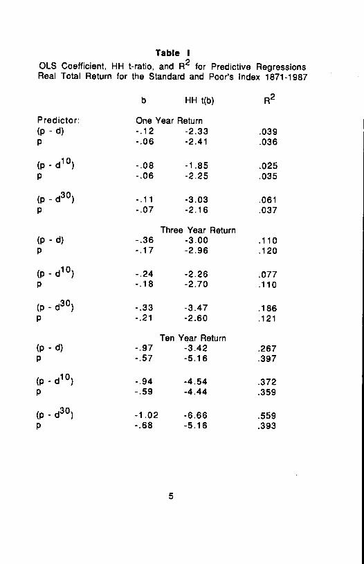
If lagged dependent variable bias is an important factor in theapparent predictive power of ratios involving price, then price by itselfshould also predict stock returns. The coefficients for the log of priceand for the log of the price/dividend ratio should both be negative,reflecting the negative bias in regression on a lagged dependent variable.In Table 1 are reported the regression coefficients, t-ratios, and R2 for aset of regressions based on those reported by Campbell and Shiller (1988)using their annual data set for the Standard and Poor's Index 1871-1987.The dependent variable is total return on the Index adjusted for inflationusing the PPI. Explanatory variables are logs of the ratio of price tolagged dividends, versions of these using 10 and 30 year moving averagesof dividends (denoted by superscripts), and the price alone. Note thatprice is measured at the beginning of year t and dividends are paid duringyear t. Return is measured alternatively over one year and overlappingthree and ten year intervals. For each combination of return andprice/dividend ratio there is a sample-matched regression on price.Following Hansen and Hodrick (1980), standard errors for t-ratios takeinto account the serial correlation induced by overlapping observations;see Appendix 1. The resulting ratio of coefficient to asymptotic standarderror is denoted HH t(b).
4
Table IOLS Coefficient, HH t-ratio, and R2 for Predictive RegressionsReal Total Return for the Standard and Poor's Index 1871-1987
b HH t(b)
Predictor: One Year Return(p - d) -.12 -2.33 .039p -.06 -2.41 .036
(p - d10) -.08 -1.85 .025p -.06 -2.25 .035
(p - d30) -.11 -3.03 .061p -.07 -2.16 .037
Three Year Return(p - d) -.36 -3.00 .110p -.17 -2.96 .120
(p - d10) -.24 -2.26 .077p -.18 -2.70 .110
(p - d30) -.33 -3.47 .186p -.21 -2.60 .121
Ten Year Return(p - d) -.97 -3.42 .267p -.57 -5.16 .397
(p - d10) -.94 -4.54 .372p -.59 -4.44 .359
(p - d30) -1.02 -6.66 .559p -.68 -5.16 .393
5
As predicted by lagged dependent variable bias, all the slopecoefficients are negative. Further, price by itself has about as much ormore explanatory power and statistical significance as do the ratios ofprice to the lagged dividends and to the 10 year moving average ofdividends. The coefficient on the price/dividend ratio is larger that onprice in every case, reflecting in part the smaller sample variance of theratio. While these features of the historical regressions are consistent indirection with the bias explanation of predictability, they are alsoconsistent with the hypothesis that price itself is a source of informationon future returns. We know of no economic motivation, however, for sucha hypothesis. Further, it would imply that expected return isnonstationary with a positive drift through time since that is true of theprice level.
Note that the longer the horizon over which return is measured, thegreater is the fraction of variation that is predicted and the stronger isthe statistical significance. The increase in R2 with return horizon hasbeen emphasized in this literature as a strong and important feature ofthe empirical evidence. However, the positive serial correlation inducedby overlapping observations would in itself tend to increase R2. Grangerand Newbold (1974) showed that the expected value of rises with thedegree of autocorrelation regardless of any relation between thevariables, creating a spurious correlation. They conclude (op cit p. 114):"Thus, a high value of R2 should not, on the grounds of traditional tests, beregarded as evidence of a significant relationship between autocorrelatedseries." The t-ratios are therefore of greater relevance in judgingwhether predictability increases with return horizon. However, sinceprice by itself shares this property with the ratios, the horizon effectmay also reflect the fact that the bias is a decreasing function of (non-overlapping) sample size which is reduced by the calculation of returnsover longer horizons. The relation of significance to horizon may alsoinvolve the small sample properties of the HH standard errors used in thecase of overlapping returns.
When the 30 year moving average of dividends used in calculatingthe price/dividend ratio it results in greater the explanatory power andstatistical significance than price alone. One consequence of a longermoving average is shortened sample size and therefore larger bias, butprice by itself in the sample-matched regressions shows no
6
correspondingly large effect. Similarly, increased small sample bias inthe HH standard errors would also have shown up in regressions on pricealone. Whether the 30 year results are too large to be attributed tosampling error depends on the unknown small sample distribution.
The next section of the paper describes a Monte Carlo experimentdesigned to investigate the extent to which the main features of thehistorical results can arise in hypothetical data where price does in factadjust fully to fundamentals and returns are not predictable.
II. Monte Carlo Estimates of Small Sample Bias
The strategy behind a Monte Carlo experiment is to generateartificial data under the null hypothesis and tabulate the empiricaldistribution of sample statistics. We take as our null hypothesis thepresent value model of stock prices which says that the price is thediscounted present value of expected dividends or net cash flow. This is,however, an incomplete specification since we need to say howinformation about the future is generated and how the term structure ofdiscount rates moves over time. The actual predictability of returns willdepend on these details of the complete specification and, as we shall see,the small sample bias in predictive regressions will also. For this reasonthere cannot be a unique bias, rather we can only report the bias foundunder particular specifications which at least account for someobservable features of the data.
To complete the null hypothesis we assume that expected future realdividends are discounted at rate r which is constant through time. Underthis specification, expected real return is of course constant through timeand equal to r. The actual predictability of real returns is zero, so anythat we find in predictive regressions is spurious. To investigate theeffect of dividend smoothing on the bias we assume a version of theLintner (1956) model with values of the smoothing parameter taken over arange suggested by the historical data. We anticipate that a smootherdividend series will produce stronger spurious predictability as theprice/dividend ratio becomes a better proxy for price.
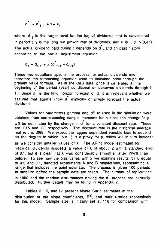
The target level of dividends toward which actual dividends adjusthas the character of a long horizon forecast. From the result of Beveridgeand Nelson (1981) it will therefore be a random walk with drift. Thegenerating process is then
7
dt=dti +y+ Ut
where dt is the target level for the log of dividends that is established
in period t, y is the long run growth rate of dividends, and u is i.i.d. N(0,2).The actual dividend paid during t depends on d and on past history
according to the partial adjustment equation
dt = dti + A (dti - dti).
These two equations specify the process for actual dividends andtherefore the forecasting equation used to calculate price through thepresent value formula. As in the C&S data, price is generated at thebeginning of the period (year) conditional on observed dividends through t-1. Since d is the long horizon forecast of d, it is irrelevant whether weassume that agents know d explicitly or simply forecast the actualdividend.
Values for parameters gamma and 2 to used in the simulation wereobtained from corresponding sample 0mt5 for p since the change in pwill be dominated by the change in d for a constant discount rate. Theseare .015 and .03 respectively. The discount rate is the historical averagereal return, .066. We expect the lagged dependent variable bias to dependon the degree to which (p-d1) is a proxy for p, which will in turn increaseas we consider smaller values of A. The AR(1) model estimated forhistorical dividends suggests a value of A of about .2 with a standard errorof 0.1, but it is clear that A was considerably smoother after WWII thanbefore. To see how the bias varies with A we examine results for A equalto 0.5 and 0.1, denoted experiments A and B respectively, representing arange that includes the point estimate. The process is given 100 periodsto stabilize before the sample data are taken. The number of replicationsis 1000 and the random disturbances driving the d process are normallydistributed. Further details may be found in Appendix 2.
Tables II, Ill, and IV present Monte Carlo estimates of thedistribution of the slope coefficients, R2, and their t-ratios respectivelyfor this model. Sample size is initially set at 116 for comparison with
8
the historical Standard and Poor's results from C&S which are tabulatedfor comparison. The dependent variable is total return over, successively,one, three and ten periods. The predictive variables are the log of theratio of price to dividends and to ten and thirty year moving averages ofdividends as well as the log of price by itself. In addition, a random walkvariable called z which is unrelated to anything else is also a used as apredictive variable to check the distributions of t-ratios computed usingthe HH correction in the case of multiperiod returns and to calibrate thedistribution of R2 (the coefficient of z having expectation zero).
9
Table II A
Empirical Distribution of the Slope CoefficientSpeed of Adjustment of Dividends: . = 0.5
Sample Size is 116
Monte Carlo: FractilesPredictor Historical Mean .025 .975
One Year Return(p-d) -.12 -.03 -.38 .26p -.06 -.04 -.12 .01
(p - d10) -.08 -.03 -.16 .07
(p - d30) - .11 - .04 - .1 7 .03
Three Year Return(p-d) -.36 -.09 -.81 .66p -.17 -.10 -.35 .02
(p - d10) -.24 -.07 -.39 .18
(p - d30) - .33 - .11 - .43 .09
Ten Year Return(p - d) -.97 -.28 -1 .58 1.44p -.57 -.31 -.88 .10
(p - d10) -.94 -.18 -.83 .56
(p - d30) -1.02 -.31 -1.06 .26
10
Table II B
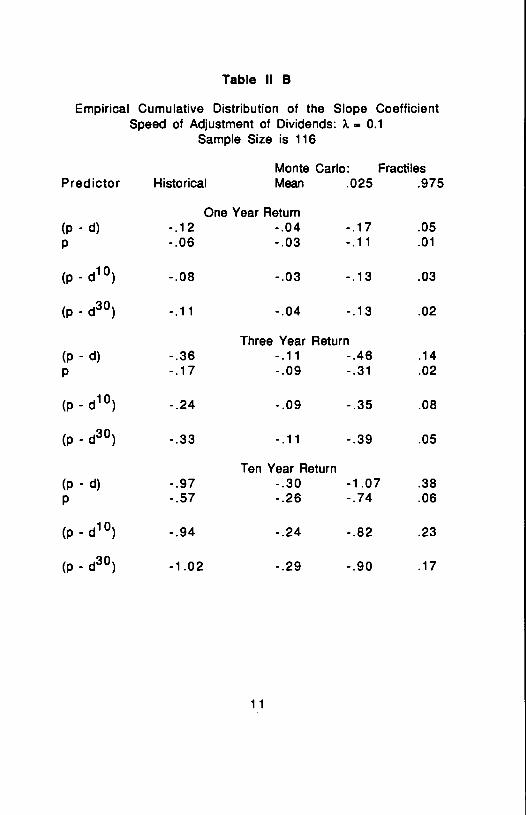
Empirical Cumulative Distribution of the Slope CoefficientSpeed of Adjustment of Dividends: . 0.1
Sample Size is 116
Monte Carlo: FractilesPredictor Historical Mean .025 .975
One Year Return(p - d) -.12 -.04 -.17 .05p -.06 -.03 -.11 .01
(p - d10) -.08 -.03 -.13 .03
(p - d30) -.11 -.04 -.13 .02
Three Year Return(p-d) -.36 -.11 -.46 .14p -.17 -.09 -.31 .02
(p - d10) -.24 -.09 -.35 .08
(p - d30) -.33 - .11 -.39 .05
Ten Year Return(p - d) -.97 -.30 -1.07 .38p -.57 -.26 -.74 .06
(p - d10) -.94 -.24 -.82 .23
(p - d30) -1.02 -.29 -.90 .17
11
Slope coefficients
The slope coefficients are negatively biased in all of theseregressions. When price level is the explanatory variable, Kendall'sapproximation, (-4/n) where sample size n is taken to be the number ofnon-overlapping observations, provides a good rule of thumb for themagnitude of the bias. For one year returns we have -0.035, for three yearreturns -0.104, and for ten year returns -0.348. Thus, reduction ineffective sample size explains why the multiperiod return regressions aremore biased than those for one period returns.
The bias in the regression on (p - d) is larger when ? is 0.1 thanwhen X is 0.5. The more smoothing there is of dividends the more (p - d)reflects variation in price and is therefore a better proxy for price. Thefractiles also show that the sampling distribution of the ratio coefficientbecomes more like that of the price coefficient with smaller values of ?..The influence of ?. on bias is smaller when the moving average of dividendsis used to calculate the ratio, presumably since dividends are smoothedanyway by the moving average. Recall that the coefficients for the ratioswere larger in magnitude than those for price in the historicalregressions. This is also the case on average in the artificial data when Xis 0.1.
Calculation of the price/dividend ratio using a moving average ofdividends evidently has offsetting effects. As we go from no smoothing tothe ten year moving average the bias decreases in magnitude. Theaveraging of dividends has a smoothing effect, tending to make the ratio abetter proxy for price, and a noise-introducing effect since variation inthe moving average involves lagged dividend innovations which areirrelevant to current price. When we go to the thirty year moving averagefrom ten years, the bias increases in magnitude. Observations are lost incalculating the moving average and the smaller sample size tends toincrease the bias.
To what degree do the sampling distributions of the Monte Carloexperiments account for the historical results? The negative signs of thecoefficients, the increase in magnitude with the horizon over which returnis measured, the coefficient for the ratio being larger than the coefficientof price alone, and the U-shaped pattern with respect to the length of themoving average of dividends are common to both. The historical
12
coefficients, however, are larger in magnitude than the Monte Carlomeans. One is outside the 95% range for A equal to 0.5 and two are outsidefor equal to 0.1; all these cases are for ten year returns with dividendaveraging. Of course, these are not statistically independent.
13
Table Ill A
Empirical Cumulative Distribution of R2Speed of Adjustment of Dividends: = 0.5
Sample Size is 116
Monte Carlo: FractilePredictor Historical Mean .95
One Year Return(p - d) .039 .009 .034p .036 .023 .065
(p - d0) .025 .011 .042
(p - d30) .061 .018 .067
z na .009 .033
Three Year Return(p - d) .110 .016 .059p .120 .066 .186
(p - d°) .077 .029 .109
(p - d30) .186 .050 .179
z na .025 .094
Ten Year Return(p - d) .267 .028 .103p .397 .197 .481
(p - d10) .372 .066 .233
(p - d30) .559 .139 .445
z na .077 .274
14
Table Ill B
Empirical Cumulative Distribution of R2Speed of Adjustment of Dividends: . — 0.1
Sample Size is 116
Monte Carlo: FractilePredictor Historical Mean .95
One Year Return(p - d) .039 .011 .042p .036 .024 .068
(p - d10) .025 .013 .047
(p - d30) .061 .021 .067
z na .008 .032
Three Year Return(p - d) .110 .031 .111p .120 .070 .184
(p - d10) .077 .038 .133
(p - d30) .186 .059 .186
z na .023 .088
Ten Year Return(p - d) .267 .082 .279p .397 .204 .490
(p - d10) .372 .101 .341
(p - d30) .559 .165 .479
z na .075 .278
15
A2
Monte Carlo estimates of the mean of for the ratios increasewith return horizon. This reflects the spurious regression phenomenonidentified by Granger and Newbold (1974) arising from the inducedpositive autocorrelation of multiperiod returns, which is confirmed bysimilar results for z (the unrelated random walk variable).
The mean also increases with the length of the moving averagefor dividends. This second effect partially reflects decreased sample sizesince sample-matched regressions on price alone (not displayed) show asimilar but less dramatic increase. It is also partially due to the ratiobecoming a better proxy for price as the length of the moving averageincreases.
Note that price by itself has more explanatory power than do theratios. The smaller value of ? makes actual dividends smoother, so again
the ratio is a better proxy for price resulting in higher mean R2.
The pattern of historical values is similar but not entirelyconsistent with the Monte Carlo sampling distribution. Historical R2 doesrise with horizon over which the return is calculated. Taking a ten yearmoving average of dividends does not increase R2 in the one and three yearregressions, but it does when we go to a thirty year moving average. Priceby itself has a larger R2 for the three and ten year returns regressions.Finally, the historical R2 for the ratios are compared to the .95 fractile ofthe sampling distribution since it is only large values of the statistic thatcontradict the null hypothesis. Note that the value of ?. has a large impact
on the .95 fractile. Historical exceed the .95 fractile for all of the tenyear, two of the three year, and one of the one year return regression whenwe assume ? is .5. When the dividend process is more smooth with ?. equalto 0.1, all but two of the ten year return results are within the range.
16
Table IV A
Empirical Cumulative Distribution of the HH t-ratioSpeed of Adjustment of Dividends: . = 0.5
Sample Size is 116
Monte Carlo: FractilesPredictor Historical Mean .025 .975
One Year Return(p - d) -2.33 -.17 -2.22 1 .85p -2.41 -1.41 -3.39 .57
(p - d10) -1.85 -.39 -2.61 1.63
(p - d30) -3.03 -.79 -2.90 1.26
z na .02 -2.03 1.99
Three Year Return(p - d) -3.00 -0.35 -2.93 1.84p -2.96 -1.76 -4.37 .58
(p - &0) -2.26 -.52 -3.09 1.87
(p - d30) -3.47 -1.05 -3.86 1.36
z na 0.01 -2.59 2.49
Ten Year Return(p - d) -3.42 -.81 -4.57 1.81p -5.16 -2.45 -6.89 1.03
(p - d'0) -4.54 -.95 -5.18 1.98
(p - d30) -6.66 -1.71 -6.83 1.68
z na .03 -3.39 3.49
17
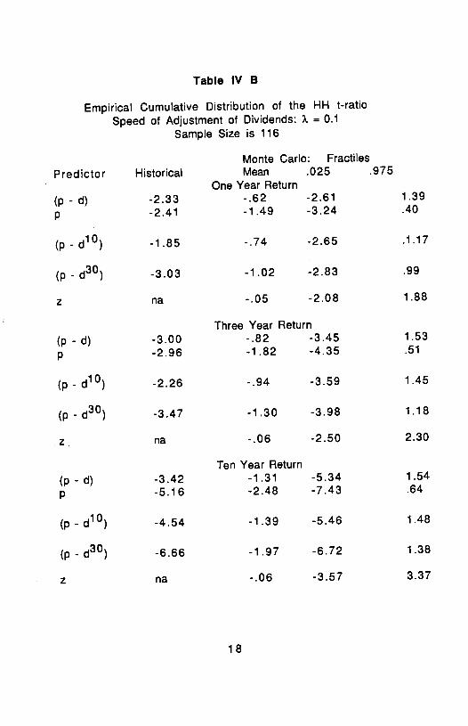
Table IV B
Empirical Cumulative Distribution of the HH t-ratioSpeed of Adjustment of Dividends: ?. = 0.1
Sample Size is 116
Monte Carlo: FractilesPredictor Historical Mean .025 .975
One Year Return
(p - d) -2.33 -.62 -2.61 1.39
p -2.41 -1 .49 -3.24 .40
(p - d10) -1.85 -.74 -2.65 .1.17
(p - d30) -3.03 -1 .02 -2.83 .99
z na -.05 -2.08 1.88
Three Year Return(p - d) -3.00 -.82 -3.45 1.53
p -2.96 -1.82 -4.35 .51
(p - d10) -2.26 -.94 -3.59 1.45
(p - d30) -3.47 -1.30 -3.98 1.18
z na -.06 -2.50 2.30
Ten Year Return
(p - d) -3.42 -1.31 -5.34 1.54
p -5.16 -2.48 -7.43 .64
(p - d10) -4.54 -1.39 -5.46 1.48
(p - d30) -6.66 -1.97 -6.72 1.38
z na -.06 -3.57 3.37
18
The t-ratio
There are two issues to be investigated with regard to the samplingdistribution of the t-ratio, which is the ratio of the OLS slope coefficientto the HH standard error. One is the negative shift in the distribution dueto the negative bias in the coefficient. The other is the appropriatenessof the HH correction for autocorrelation induced by overlappingmuftiperiod returns. To isolate the latter effect we included z, theunrelated random walk series, as another predictor of returns.
The distribution of the t-ratio for the case of autoregression whenthe data are a driftless gaussian random walk has been investigated byDickey (1976), Fuller (1976) and Dickey and Fuller (1979), and it iscentered around roughly -1 .5 for any sample size larger than 25. This isessentially what we see in Table IV for the regression of one year returnon lagged price and estimated fractiles also compare closely with Table8.5.2 of Fuller (1976). The rate of drift of the price series is not largeenough to have an important effect on the distribution along the linessuggested by Evans and Savin (1984). We expect that the effect of aslower rate of adjustment of dividends will be to make the distribution ofthe t-ratio for the price/dividend ratio more like that for price by itself.This is what we see in Table IV as a slower speed of adjustment or alonger moving average is considered.
A multiperiod horizon for the return introduces positiveautocorrelation in the residuals which the HH correction is designed totake into account. If we did not use the correction then standardeconometric theory leads us to expect too large a dispersion for the t-ratio, but if the correction is successful the range between the .025 and.975 fractiles should be roughly 4. What we see in Table IV is that thisrange increases to about 5 for three year returns and to about 7 or 8 forten year returns. Since the z variable shows the same pattern thespreading is clearly due to the HH adjustment to the standard error notbeing large enough to correct for autocorrelation. Of course, the HHstandard errors would be correct asymptotically so this can be viewed asanother small sample bias.
While the historical t-ratios are larger in magnitude than thesampling means, they are generally within the .025-.975 range. With X at0.5 there are three exceptions, and with ). at 0.1 the single exception isfor the regression of the one year return on the ratio which uses the 30
19
year moving average of dividends. The difference between taking thehistorical t-ratios at face value and taking them as drawings from thesampling distributions of this experiment is the difference between asignificance level around .05 and one that is infinitesimal. Equivalently,it is the difference between a test statistic that is about two standarddeviations from the mean and one that is 3 to 6.
Ill. Larger Sample Size and Monthly Data
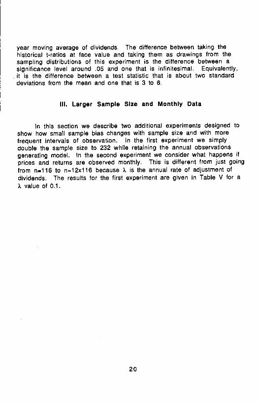
In this section we describe two additional experiments designed toshow how small sample bias changes with sample size and with morefrequent intervals of observation. In the first experiment we simplydouble the sample size to 232 while retaining the annual observationsgenerating model. In the second experiment we consider what happens ifprices and returns are observed monthly. This is different from just goingfrom n=116 to n=12x116 because ? is the annual rate of adjustment ofdividends. The results for the first experiment are given in Table V for a? value of 0.1.
20
Table V
Empirical Means of the Slope, R2, and HH t-ratioSpeed of Adjustment of Dividends: = 0.1
One Period Return(p - d) - .04 - .02 .011 .005 -.62 -.46p -.03 -.01 .024 .009 -1.49 -1.15
(p - d10) -.03 -.01 .013 .005 -.74 -.52
(p - d30) -.04 -.01 .021 .007 -1.02 -.68
z .008 .004 -.05 ..05
Three Period Return(p - d) -.11 -.05 .031 .014 -.82 -.57p -.09 -.03 .070 .026 -1.82 -1.35
(p - d10) -.09 -.04 .038 .016 -.94 -.63
(p - d30) -.11 - .04 .059 .020 -1.30 -.82
z .023 ..013 -.06 ..06
Ten Period Return(p - d) - .30 -.16 .082 .037 -1.31 -.79p -.26 -.09 .204 .085 -2.48 -1.61
(p - d10) -.24 -.12 .101 .044 -1.39 -.81
(p - d30) -.29 -.12 .165 .060 -1.97 -1.03
z .075 ..044 -.06 ..06
21
The work of Dickey, Fuller and Evans and Savin give some guidanceabout what we should expect to see when the number of annualobservations is doubled. For regression on the lagged level of a driftlessrandom walk we know that the bias is proportional to 1/n, and the resultsof Evans and Savin (1984) suggest that the bias will decrease faster inthe presence of a nonzero expected change. The bias for the coefficient oflagged price is indeed about a third as large when n is doubled, and thereis a similar decrease for the price/dividend ratio. The t-ratio isessentially independent of sample size in the driftiess random walk case,and this implies that R2 will decline in proportion to 1/n. We see in TableV that the decline in mean R2 is somewhat faster than this, relecting adecline in mean t-ratios with the doubling of n. These results suggestthat the erroneous inference of predictability becomes less of a problemas sample size grows.
Recall that the sampling variance of the t-ratio was also too largefor three and ten year returns because the HH correction for overlappingobservations was not large enough. Fractiles of the t-ratio which are notshown confirm that the sampling distribution is also becoming lessdisperse with sample size, although it is still too large. For n=116 thedistances between the .025 and .975 fractiles were approximately 4, 5,and 7 for one, three and ten year returns respectively when theindependent variable was (p-d). For n232 these distances becomeapproximately 4, 4.8, and 5.5. A similar pattern was also found when thepredictive variable was the unrelated random walk z. Thus thecontribution of overlapping observations to the inference of predictabilityyields only slowing to increasing sample size.
In the second experiment we consider the whether monthlyobservations instead of annual mitigate small sample bias. The datagenerating mechanism has the same form as that for annual data exceptthat the target dividend process is monthly with drift and variance onetwelfth as large. Actual dividends adjust toward the target at onetwelfth the annual rate (?.) and price is calculated from the discountedpresent value of expected future divdiends each month. We have12x1161392 monthly observations on total return, the log of price, andthe price/dividend ratio. Results for one period return regressions arereported in Table VI.
22
Table VI
Empirical Distribution of the Slope, R2, and HH t-ratioAnnual Speed of Adjustment of Dividends: = 0.1
Sample Sizes are 116 Years and 1392 (12x116) Months
Note that the distribution of the t-ratio is essentially the same inmonthly data as it is in annual data. Observing the process at monthlyintervals instead of annual does not alter the apparent statisticalevidence for predictability. This is consistent with the insensitivity ofthe distribution of the t-ratio to sample size reported by Dickey (1976) inautoregressions with unit roots. While the monthly observations multiplythe number of independent observations by 12, that is irrelevant. Therelevant difference is that we are observing the same nonstationaryprocess 12 times more frequently, running what amounts to anautoregression as explained in the introduction, and that does notsubstantially alter our inferences about the process. The values of R2 areproportionally smaller for monthly data in accordance with the algebraicrelation between t and R2. Of course the slope coefficient is about onetwelfth as large for monthly data since the corresponding predicted returnis at a montly rate.
Fama and French (1988) reported t-ratios in the range of 1 .15 to2.76 for regressions of the monthly returns from the CRSP tapes 1926-86on the the raw dividend yield. We intend to run a further experiment thatis more directly comparable to their regression, however based on theabove experiment we would not expect that the reported t-ratios are asstrongly significant as they had appeared.
IV. Summary and Conclusions
A number of recent studies have reported that stock returns can bepredicted to a statistically significant degree by fundamentals and thatpredictability increases as one considers returns over multiperiodhorizons. In this paper we have looked at whether these findings could tosome degree be attributed to small sample biases. Regression on a laggeddependent variable is subject to small sample bias and this suggests thatregression of stock returns on the price/dividend ratio or similar valuemeasures involving price may be subject to a related bias. Further,multiperiod returns are by construction positively autocorrelated,suggesting the possibility of spurious regression as another source ofapparent predictability. To investigate the size and economic significanceof these biases we have run a Monte Carlo experiment in which prices andreturns are generated by a version of the present value model in which
24
expected returns are constant. While the generating model replicatessome features of the distribution of historical annual real returns since1871, it is not the only specification of the present value model nor theonly one with constant expected returns. A different specification of thenull hypothesis would presumably imply somewhat different biases.
Under the specification we have chosen, a number of the features ofthe historical regression results arise as the consequence of small samplebiases: reliably negative coefficients on the price/dividend ratio whichseems to suggest one can buy low and sell high, an increase in A2 asreturns are calculated over longer horizons, and the apparent increase instatistical significance as longer horizons and more dividend averagingare used. Judging the statistical significance of regressions withmultiperiod returns requires an appropriate upward adjustment ofstandard errors due to the induced autocorrelation. We find that thecorrection based on asymptotic theory is not large enough in smallsamples, resulting in spuriously large t-ratios.
Generating monthly data of equivalent length in years, we find thatstatistical inferences are essentially the same as in annual data.Although it would seem that one would have twelve times the number ofindependent observations, the relevant analogy is to taking observationson a nonstationary series twelve times as frequently. The latter does notchange greatly inferences about the process.
The magnitude of the historical results reported for annual returnsby Campbell and Shiller (1988) and monthly returns by Fama and French(1988) is such that they cannot be dismissed entirely as the result ofsmall sample bias under our generating model. Their statisticalsignificance, however, would seem to be substantially weaker than iftaken at face value.
25
REFERENCES
Beveridge, Stephen and Charles R. Nelson, 1981, A new approach to thedecomposition of economic time series into permanent andtransitory components with particular attention to measurement ofthe "business cycle," Journal of Monetary Economics 7, 151-174.
Campbell, John Y., and Robert J. Shiller, 1988, Stock prices, earnings, andexpected dividends, The Journal of Finance 43, 661-676.
Cecchetti, Stephen G., P0k-sang Lam, and Nelson C. Mark, 1990, Meanreversion in equilibrium asset prices, American Economic Review80, ??.
Cutler, David M., James M. Poterba, and Lawrence H. Summers, 1989,Speculative Dynamics, paper presented at London School ofEconomics conference on econometrics of financial markets, June1989.
Dickey, David A. and Wayne A. Fuller, 1979, Distribution of the estimatorsfor autoregressive time series with a unit root, Journal of theAmerican Statistical Association 74, 427-431.
Dickey, David A., 1976, Estimation and hypothesis testing in nonstationarytime series, Ph.d. dissertation, Iowa State University.
Evans, G. B. A. and N. E. Savin, 1984, Testing for Unit Roots: 2,Econometrica 52, 1241-1269.
Fama, Eugene F. and Kenneth A. French, 1988, Dividend yields and expectedstock returns, Journal of Financial Economics 22, 3-25.
Fuller, Wayne A., 1976, Introduction to Statistical Time Series (JohnWiley, New York).
Granger, C. W. J. and P. Newbold, 1974, Spurious regressions ineconometrics, Journal of Econometrics 2, 111-120.
Hansen, Lars Peter, and Robert J. Hodrick, 1980, Forward Exchange ratesas optimal predictors of future exchange rates: an econometricanalysis, Journal of Political Economy 88, 829-853.
26
Kendall, M. G., 1954, Note on bias in the estimation of autocorrelation,Biometrika 41, 403-404.
Keim, Donald and Robert Stambaugh, 1986, Predicting Returns in the Stockand Bond Markets, Journal of Financial Economics 17, 357-390.
Kim, Myung-Jig, Charles A. Nelson and Richard Startz, 1989, Meanreversion in stock prices: a reappraisal of the empirical evidence,NBER Working Paper No. 2795.
Lintner, John, 1956, Distribution of income of corporations amongdividends, retained earnings and taxes, American Economic Review46, 97-113.
Newey, Whitney K., and Kenneth D. West, 1987, A simple, positive semi-definite, heteroskadasticity and autocorrelatio n consistentcovariance matrix, Econometrica 55, 703-708.
Phillips, P. C. B., 1987, Time series regression with a unit root,Econometrica 55, 277-301.
Poterba, James M. and Lawrence H. Summers, 1988, Mean reversion instock prices, Journal of Financial Economics 22, 27-59.
Shiller, Robert J., 1981, Do stock prices move too much to be justified bysubsequent changes in dividends, American Economic Review 75,421 -436.
White, Halbert, 1980, A heteroskedasticity-consistent covariance matrixestimator and a direct test for heteroskedasticity, Econometrica 48,8 17-838.
27
Appendix 1: The Correction for the Standard Errors in the Multiyear Returns
Regression
Our procedure of calculating the standard errors is in the spirit of White's [19801 consistent
estimators for the covariance matrix of estimators. That is, the asymptotic covariance matrix of
$K in the regression of K-multiyear returns (rt,,+K) on the predictor X can be estimated from
=
where X = (x1, ,zr)', Ur = (u1, ,UT)' and i,'s are the least square residuals. As is shown in
H&H, the T by T matrix UTU. will include not only the T-elements main diagonal, but also K-I off-
diagonal terms (pararell to the main diagonal) reflecting the (K-1)th order serial correlations induced
by overlapping data, and zeros elsewhere. The difference between the original H&H correction and
ours lies in that H&H imposed equality along the diagonals. in fact the standard errors estimated
from both methods are very close. C&S reported SE's of .0570, .1443 and .2997 from the regression
of 1, 3 and 10-year returns on the dividend-price ratio, while the White version estimates .0529,
.1183 and .2843, respectively.
When there are large negative sample serial covariances the variances can take on negative
values. To ensure the positive definiteness of the variances the nonzero off-diagonal terms may
be modified by multiplying those by the arithematically declining weights proposed by Newey and
West [1987] and Phillips 11987]. Thus the modification may be written as
T K—i TX.UTU.XT = ugxzu + 2. (1 —
+ fl+Iand the t-statistics based on the modified standard error are calculated in the Monte Carlo simu-
lation and are reported as HHt(b) in the paper.
1
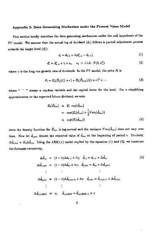
Appendix 2: Data Generating Mechanism under the Present Value Model
This section briefly describes the data generating mechanism under the null hypothesis of the
PV model. We assume that the actual log of dividend (di) follows a partial adjustment process
towards the target level (di):
d = d_1 + \(d..1 — d_1) (1)
= d_1 + + U, Uj — :.i.d. N(O, ) (2)
where y is the long run growth rate of dividends. In the PV model, the price P is
P = E(D)/(l + r) + E(D1+1)/(1 + r)2 +.. (3)
where " " means a random variable and the capital letter for the level. For a simplifying
approximation to the expected future dividend, we note
E(D+1) = E, exp{J,+,}
= exp{E(J÷,) + Var(J+)}
exp{Et(+1)} (4)
since the density function for A÷. is log-nonnal and the variance Var(d1+1) does not vary over
time. Now let d÷ denote the expected value of at the beginning of period t. Similarly,
= Using the ARI(1,1) model implied by the equation (1) and (2), we construct