1 Atomistic Molecular Dynamics Simulations of Carbon Dioxide Diffusivity in n-Hexane, n-Decane, n-Hexadecane, Cyclohexane and Squalane Othonas A. Moultos 1 , Ioannis N. Tsimpanogiannis 1,2 , Athanassios Z. Panagiotopoulos 3 , J. P. Martin Trusler 4 and Ioannis G. Economou 1,* 1 Chemical Engineering Program, Texas A&M University at Qatar, P.O. Box 23874, Doha, Qatar 2 Environmental Research Laboratory, National Centre for Scientific Research “Demokritos”, 15310 Aghia Paraskevi Attikis, Greece 3 Department of Chemical and Biological Engineering, Princeton University, Princeton, NJ 08544, USA 4 Department of Chemical Engineering, Imperial College London, South Kensington Campus, London, SW7 AZ, United Kingdom * Corresponding author at: [email protected]For publication in the Journal of Physical Chemistry B November 2016
Transcript
1
Atomistic Molecular Dynamics Simulations of Carbon Dioxide Diffusivity in n-Hexane, n-Decane, n-Hexadecane, Cyclohexane
and Squalane
Othonas A. Moultos1, Ioannis N. Tsimpanogiannis1,2, Athanassios Z. Panagiotopoulos3, J. P. Martin Trusler4 and Ioannis G. Economou1,*
1Chemical Engineering Program, Texas A&M University at Qatar, P.O. Box 23874, Doha, Qatar
2Environmental Research Laboratory, National Centre for Scientific Research
For publication in the Journal of Physical Chemistry B
November 2016
2
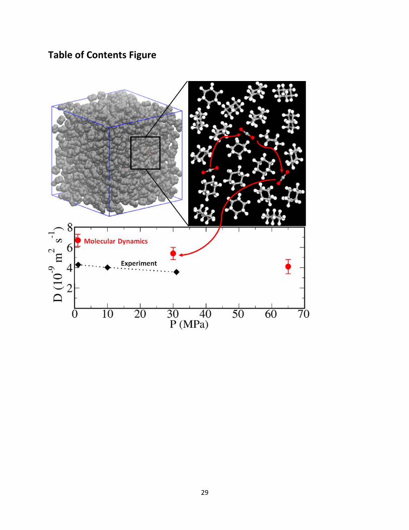
Abstract Atomistic molecular dynamics simulations were carried out to obtain the diffusion coefficients of CO2 in n-hexane, n-decane, n-hexadecane, cyclohexane and squalane at temperatures up to 423.15 K and pressures up to 65 MPa. Three popular models were used for the representation of hydrocarbons: the united atom TraPPE (TraPPE-UA), the all-atom OPLS, and an optimized version of OPLS, namely L-OPLS. All models qualitatively reproduce the pressure dependence of diffusion coefficient of CO2 in hydrocarbons measured recently, and L-OPLS was found to be the most accurate. Specifically for n-alkanes, L-OPLS also reproduced the measured viscosities and densities much more accurately than the original OPLS and TraPPE-UA models, indicating that the optimization of the torsional potential is crucial for the accurate description of transport properties of long chain molecules. The three force fields predict different microscopic properties such as mean square radius of gyration for the n-alkane molecules and pair correlation functions for the CO2 – n-alkane interactions. CO2 diffusion coefficients in all hydrocarbons studied are shown to deviate significantly from the Stokes-Einstein behavior.
1. Introduction The diffusion coefficient of CO2 in hydrocarbons is a fundamental transport property that
is encountered in a number of industrial applications. The following two characteristic examples are of particular interest to the current study: (i) During tertiary oil recovery, CO2 is injected in the oil reservoir in order to reduce the viscosity and increase the mobility of the in-situ oil as part of the enhanced oil recovery process,1 (ii) In order to mitigate global climate change associated with the uncontrolled release of CO2 in the atmosphere, the capture and sequestration of CO2 has been under extensive study as a possible solution.2 One of the most promising technologies for this is injection of CO2 in depleted oil reservoirs. In both examples, accurate models for the prediction of diffusion coefficients of CO2 in various hydrocarbons that make up the oil in the subsurface reservoirs are essential in order to design the appropriate processes, but only limited experimental measurements can be found in the open literature,3-16 with the majority of them focusing on conditions in the neighborhood of 298 K and 0.1 MPa. Design of oil recovery and carbon sequestration processes requires knowledge of the diffusion coefficients at higher pressure and temperature conditions.
Theoretical approaches for estimating diffusion coefficients have been proposed in the form of semi-empirical correlations. Models based either on the kinetic theory of Chapman and Enskog17-20 or the hydrodynamic theory of Stokes and Einstein,19-21 are popular for such calculations. However, they are not easily generalizable to many fluids and require a rich database of experimental measurements to establish their parameters. An alternative to theoretical models are atomistic molecular dynamics (MD) simulations, which have been used extensively for the calculation of transport coefficients and thermodynamic properties.22
3
The successful implementation of MD simulations depends on the accurate description of the intra- and intermolecular interactions. A large number of molecular models describing those interactions have been proposed — these are also known as “force fields”. Two popular non-polarizable CO2 force fields are the “elementary physical model” (EPM2) by Harris and Yung,23 which gives reasonable agreement with experimental data for a variety of properties, and the “transferable potential for phase equilibria” (TraPPE) by Potoff and Siepmann,24 which accurately reproduces pure CO2 phase behavior and yields satisfactory results for mixtures with n-alkanes.24 More details about these and other CO2 models are discussed in the studies by Jiang et al.25 and Moultos et al.26-28
Two of the most widely used force fields for hydrocarbons are the “optimized potentials for liquid simulations” (OPLS) model developed by Jorgensen and co-workers29-32 and the TraPPE model by Siepmann and co-workers.33-34 Particularly, OPLS-AA29-30 is an explicit hydrogen model, with most of parameters adopted from the united-atom OPLS31-32 and AMBER force fields,35 which yields very good agreement with experimental data on thermodynamic properties for many organic molecules including alkanes, alkenes, alcohols and many other. On the other hand, TraPPE-UA is a united atom model which describes accurately the vapor-liquid coexistence curves and the critical properties of linear alkanes. Although, there is an explicit hydrogen version of the TraPPE model (TraPPE-EH),34 it is not commonly considered for the calculation of transport properties, as it was designed for improved phase equilibria calculations. Very recently Siu et al.36 reported a new force field for long alkanes, the L-OPLS (“L” stands for “Long”). This model is an optimized form of OPLS-AA that provides better results for liquid properties of long hydrocarbons. Siu et al. re-optimized (a) the torsional parameters by fitting to gas-phase ab initio energy profiles, (b) the energy parameter of the Lennard-Jones (LJ) potential for methylene hydrogen atoms, and (c) the partial charges.36 Discussion on other molecular models for alkanes can be found in Paul et al.37 and Ungerer et al.38
In the current study, we performed an extensive series of MD simulations for the determination of diffusion coefficient of CO2 in five hydrocarbons: n-hexane, n-decane, n-hexadecane, cyclohexane and squalane, at infinite dilution conditions, at 298.15, 323.15 and 423.15 K and at 1, 30 and 65 MPa. This can be considered the first step towards calculating the diffusion coefficient of CO2 in real mixtures of hydrocarbons. This study is motivated by the recent availability of experimental measurements by Cadogan et al.15 and Cadogan16 covering a broad range of temperatures and pressures. The main objective of the work is the assessment of the accuracy of the force fields discussed above to predict the diffusion coefficients of CO2 in the hydrocarbons. There is a limited number of prior MD studies for such systems.39-41 In addition, liquid densities and shear viscosities of the hydrocarbons are calculated from MD simulations and are compared with available experimental data, in order to rationalize the observed trends in the prediction of diffusion coefficients of CO2, which strongly depend on the transport properties of the medium. In parallel, the mean square radius of gyration of the three n-alkanes at 323.15 K and the pair correlation function for CO2 – n–alkane are calculated for the three force fields, so that a microscopic understanding is developed in order to justify the differences in the physical
4
property values. Finally, the MD results are utilized to examine the validity of the Stokes-Einstein theory.
2. Models and methods 2.1 Intermolecular potentials. In this study, the TraPPE24 force field was used for the representation of CO2 molecules. Our early calculations using the EPM223 model for CO2 resulted in very similar values, indicating that the two force fields predict similar transport properties of CO2 in mixtures with hydrocarbons. TraPPE is a rigid linear three-site model in which the electrostatic contributions are implemented by negative partial charges fixed on the oxygen atoms and a positive one on the carbon atom.
For modelling the linear alkanes (n-hexane, n-decane and n-hexadecane) three different molecular models were employed; the united-atom TraPPE (TraPPE-UA),33 the all-atom OPLS (OPLS-AA)29-30 and the L-OPLS.36 For cyclohexane and squalane, only TraPPE and OPLS-AA were used since no L-OPLS parameters are currently available for cyclic or branched alkanes. In TraPPE-UA model, CH4, CH3 and CH2 groups are modelled as different pseudo atoms with no charges. For the case of OPLS-AA and L-OPLS models, partial positive charges are assigned to the hydrogen sites and negative to the carbon ones.
2.1.1 Bonded interactions. In general, bond stretching and bond angle bending interactions are calculated from the expressions:
𝑈𝑈𝑏𝑏𝑏𝑏𝑏𝑏𝑏𝑏(𝐫𝐫) =𝑘𝑘𝑟𝑟2
(𝐫𝐫 − 𝐫𝐫0)2 (1)
𝑈𝑈𝑎𝑎𝑏𝑏𝑎𝑎𝑎𝑎𝑎𝑎(𝜃𝜃) =𝑘𝑘𝜃𝜃2
(𝜃𝜃 − 𝜃𝜃0)2 (2)
where 𝑘𝑘𝑟𝑟 and 𝑘𝑘𝜃𝜃 are the force constants,42 while 𝑟𝑟0 and 𝜃𝜃0 are the equilibrium bond length and bond angle, respectively. For the case of TraPPE-UA, all pseudo-atoms along the alkane chain are connected with bonds of fixed length,24 while in L-OPLS force field only bonds involving hydrogens are of fixed length. For the case of OPLS-AA all bonds are flexible. Preliminary calculations using a variation of TraPPE-UA model,41 with flexible bonds resulted in almost identical diffusion coefficient values with the ones obtained from the original TraPPE-UA33 and thus they are not reported in this study. Torsional energy in the n-alkane chains is described by the Ryckaert – Bellemans (RB) potential for all the models examined:43-44
𝑈𝑈𝑡𝑡𝑏𝑏𝑟𝑟𝑡𝑡𝑡𝑡𝑏𝑏𝑏𝑏(𝜙𝜙) = �𝑐𝑐𝑏𝑏[𝑐𝑐𝑐𝑐𝑐𝑐 (𝜓𝜓)]𝑏𝑏5
𝑏𝑏=0
(3)
where 𝜙𝜙 is the dihedral angle, 𝜓𝜓 = 𝜙𝜙 − 180ο and 𝑐𝑐𝑏𝑏 is constant.
5
2.1.2 Non-bonded interactions. The non-bonded intra- and intermolecular interactions are represented by the summation of the 12 – 6 LJ repulsion-dispersion and the Coulombic interactions:
𝑈𝑈𝑏𝑏𝑏𝑏�𝑟𝑟𝑡𝑡𝑖𝑖� = 4𝜀𝜀𝑡𝑡𝑖𝑖 ��𝜎𝜎𝑡𝑡𝑖𝑖𝑟𝑟𝑡𝑡𝑖𝑖�12
− �𝜎𝜎𝑡𝑡𝑖𝑖𝑟𝑟𝑡𝑡𝑖𝑖�6
� +𝑞𝑞𝑡𝑡𝑞𝑞𝑖𝑖
4𝜋𝜋𝜀𝜀0𝑟𝑟𝑡𝑡𝑖𝑖 (4)
where 𝜀𝜀𝑡𝑡𝑖𝑖, 𝜎𝜎𝑡𝑡𝑖𝑖, and 𝑟𝑟𝑡𝑡𝑖𝑖 are the LJ energy parameter, the LJ size parameter, and the distance between atoms i and j, respectively, and 𝜀𝜀0 is the vacuum permittivity. In the TraPPE model, the intramolecular 1 – 4 interactions are excluded,33 while in the OPLS-AA and L-OPLS 1 – 4 interactions are scaled by a factor of 0.5, both for the LJ and Coulombic interactions.42 Interactions between unlike atoms in the TraPPE force field are computed using the Lorenz–Berthelot (LB) combining rules:22
𝜀𝜀𝑡𝑡𝑖𝑖 = �𝜀𝜀𝑡𝑡𝜀𝜀𝑖𝑖�12 (5)
𝜎𝜎𝑡𝑡𝑖𝑖 =12�𝜎𝜎𝑡𝑡 + 𝜎𝜎𝑖𝑖� (6)
while for OPLS-AA and L-OPLS 𝜀𝜀𝑡𝑡𝑖𝑖 is calculated from eq. (5) and 𝜎𝜎𝑡𝑡𝑖𝑖 from: 4
𝜎𝜎𝑡𝑡𝑖𝑖 = �𝜎𝜎𝑡𝑡𝜎𝜎𝑖𝑖�12 (7)
Preliminary simulations with TraPPE were performed using the geometric combining rule for 𝜎𝜎𝑡𝑡𝑖𝑖 instead of the arithmetic one (Eq. 6), but no appreciable differences were detected for 𝐷𝐷𝐶𝐶𝐶𝐶2 in various n-alkanes. On the other hand, phase equilibrium calculations have been shown to be more sensitive on the combining rules used.45-48 The values of all the bonded and non-bonded parameters of the force fields used in the present study are listed in Table S1 and S2 of the Supporting Information, for the hydrocarbons and CO2, respectively.
2.2 Computational details. All MD simulations were carried out with the open-source package GROMACS49-50 (Version 4.6.5), in cubic boxes with periodic boundary conditions imposed in all directions. The general simulation scheme was the following: Initially the alkane and CO2 molecules were placed randomly in the box and were allowed to equilibrate in the isothermal-isobaric (NPT) ensemble for 1 – 4 ns. During this period, the density of the system and the radii of gyration of hydrocarbons converged to mean values. Subsequently, all properties of interest were calculated from 50 – 100 ns NPT production runs. In all MD simulations the long-range electrostatic interactions were treated by the particle mesh Ewald (PME)51-52 method and mean-field tail corrections were applied for the energy and pressure.22
For the TraPPE-UA simulations, the time step was set to 2 fs, while the temperature and pressure were maintained constant using the Nosé-Hoover53-54 thermostat and Parrinello-
6
Rahman55 barostat respectively, with coupling constants equal to 1 ps. The cut-off distance was set to 14 Å, both for the LJ and real space components of the PME. For the OPLS-AA and L-OPLS simulations, the velocity rescaling56 method was used for thermostating, while the system pressure was coupled isotropically by the Parrinello-Rahman55 barostat with time constants equal to 2 and 4 ps respectively. The van der Waals interactions were treated using a switch function57 between 11 – 13 Å. For the simulations involving the OPLS-AA model, the time step used was 1 fs, while for L-OPLS the time step was 2 fs, as in the original L-OPLS paper.36
2.3 Diffusion coefficient and viscosity calculations. The diffusion coefficients of CO2 in hydrocarbons, 𝐷𝐷𝐶𝐶𝐶𝐶2, were calculated using the Einstein’s relation, according to which the diffusion coefficient is the slope of the mean square displacement: 22, 58
𝐷𝐷𝐶𝐶𝐶𝐶2 = lim𝑡𝑡→∞
⟨[𝐫𝐫𝑡𝑡(0) − 𝐫𝐫𝑡𝑡(t)]2⟩6𝑡𝑡
(8)
where 𝐫𝐫𝑡𝑡(𝑡𝑡) is the coordinate vector for the solute molecule i center of mass at time t, and the angle brackets indicate an ensemble average over all solute molecules and time origins. In order to achieve low statistical uncertainties each state point was calculated by averaging the results of 20 independent simulations, each one starting from a different initial configuration. For the calculation of shear viscosity, the Green-Kubo relation was used:22, 59
𝜂𝜂(𝑡𝑡) =𝑉𝑉𝑘𝑘𝐵𝐵𝑇𝑇
� ⟨𝑃𝑃𝛼𝛼𝛼𝛼(𝑡𝑡0)𝑃𝑃𝛼𝛼𝛼𝛼(𝑡𝑡0 + 𝑡𝑡)⟩ 𝑑𝑑𝑡𝑡∞
0 (9)
where V is the volume of the simulation box and the angle brackets indicate an ensemble average over all time origins. Pαβ denotes the off-diagonal elements of the pressure tensor:
𝑃𝑃𝛼𝛼𝛼𝛼 =1𝑉𝑉�
𝑃𝑃𝑡𝑡𝛼𝛼𝑃𝑃𝑡𝑡𝛼𝛼𝑚𝑚𝑡𝑡𝑡𝑡
+ ��𝑟𝑟𝑡𝑡𝑖𝑖𝑎𝑎𝑓𝑓𝑡𝑡𝑖𝑖𝛼𝛼𝑡𝑡>𝑖𝑖𝑡𝑡
(10)
where 𝑚𝑚𝑡𝑡 is the molecular mass, 𝑟𝑟𝑡𝑡𝑖𝑖𝑎𝑎 is the 𝛼𝛼-component of the position vector 𝒓𝒓𝑡𝑡 − 𝒓𝒓𝑖𝑖 and 𝑓𝑓𝑡𝑡𝑖𝑖𝛼𝛼 is the 𝛽𝛽-component of force on atom i due to atom j. In order to reduce the statistical uncertainty, we averaged the autocorrelation functions over all independent off-diagonal tensor elements 𝑃𝑃𝑥𝑥𝑥𝑥, 𝑃𝑃𝑥𝑥𝑥𝑥, 𝑃𝑃𝑥𝑥𝑥𝑥; because of rotational invariance we also added the equivalent �𝑃𝑃𝑥𝑥𝑥𝑥 – 𝑃𝑃𝑥𝑥𝑥𝑥�/2 and �𝑃𝑃𝑥𝑥𝑥𝑥 – 𝑃𝑃𝑥𝑥𝑥𝑥�/2 terms.54 The pressure components were sampled every 5 fs. Viscosity at each temperature and pressure was calculated by averaging 5 independent simulations. This number of independent simulations was proven sufficient to obtain relatively low statistical uncertainties (1% - 9%), while in the same time keeping the output files’ size within manageable levels (1 - 5 gigabytes). In this work, for all viscosity simulations, 300 molecules were used.
The number of CO2 solutes in simulations with TraPPE-UA n-hexane, n-decane, n-hexadecane and cyclohexane was set equal to 5, while the number of solvent molecules was
7
1,000. For simulations of TraPPE squalane, and OPLS-AA and L-OPLS alkanes the number of CO2 molecules in the system was 3, while the solvent molecules were 300. These system sizes result in a mole fraction for CO2 in the range of 0.005 – 0.01. The reason that more than one CO2 molecules were used was to enhance the statistical accuracy of the calculated diffusivities. The conditions studied still correspond to near infinite-dilution conditions, as solute-solute interactions are negligible. In order to ensure that the effects of solute-solute interactions are negligible, simulations of systems with 1, 3 and 5 CO2 molecules dissolved in 1,000 n-hexane, n-decane or n-hexadecane molecules, using the TraPPE-UA force field were performed. The results are shown in Figure S1a in the Supporting Information. The values of 𝐷𝐷𝐶𝐶𝐶𝐶2for the three systems almost coincide within their respective uncertainties, indicating that there is no effect of concentration in this range on the diffusion coefficient calculations. Additionally, the statistical uncertainty of 𝐷𝐷𝐶𝐶𝐶𝐶2 calculated from the system with the 5 molecules is significantly smaller.
According to the literature,28,60,76 self-diffusion coefficients of pure components vary linearly with inverse system size. In Figure S1b the diffusion coefficient of CO2 is plotted as a function of 𝑁𝑁−1/3 , where 𝑁𝑁 is the number of solvent molecules of linear n-alkanes. System sizes with 125, 250, 500, 1000 and 2000 solvent molecules were examined for n-hexane, n-decane and n-hexadecane with the TraPPE force field. Given the statistical uncertainties in the diffusivity values (5 % – 18 %), system size dependences cannot be easily detected. These results are in line with our previous studies of the H2O – CO2 mixture.27-28
3. Results and discussion
3.1 Diffusion coefficient of CO2 in linear alkanes. In an earlier study we showed that the TraPPE CO2 force field predicts the self-diffusion coefficient of pure CO2 very accurately, exhibiting absolute deviations from the experimental data lower than 2.4 %.28 At the same time, it yields satisfactory results for the diffusivity calculations of the binary H2O – CO2 mixture, when combined with appropriate H2O force fields, for a wide range of temperatures and pressures.27-
28
In a recent study, Cadogan et al.15 reported experimental measurements for infinitely diluted CO2 in various alkanes (n-hexane, n-heptane, n-octane, n-decane, n-dodecane, n-hexadecane and squalane) obtained by the Taylor Dispersion method.61 In the present work, we focus on simulations of the diffusion coefficients of infinitely diluted TraPPE CO2 in most of these alkanes, namely: n-hexane, n-decane, n-hexadecane, cyclohexane and squalane. The intermediate-length linear alkanes are expected to follow similar trends as the systems studied here.
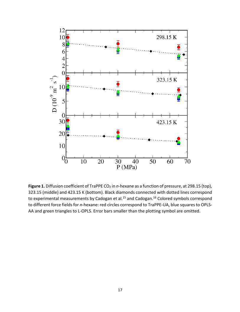
The MD results for CO2 diffusion coefficient, 𝐷𝐷𝐶𝐶𝐶𝐶2, in n-hexane at 298.15, 323.15 and 423.15 K are listed in Table 1 and plotted in Figure 1 as a function of pressure. Over the range of temperatures and pressures examined, simulations with the TraPPE-UA model yield the least
8
accurate results, with deviations from the experimental data in the range 19% – 65%, and with an average absolute deviation (AAD) for all temperature and pressures approximately equal to 28%. The results are drastically improved with the OPLS-AA force field. For the same conditions, the diffusion coefficients of CO2 in n-hexane deviate from experimental data by 1% – 28%, with an AAD equal to 13%. L-OPLS model appears to be the most accurate one, with deviations from experimental data being less than 9% for all conditions studied, except for 423.15 K and 1 MPa. One should notice that at the particular state point of 423.15 K and 1 MPa, which corresponds to the lowest density considered, all models examined showed the least accurate behavior. Earlier studies for pure n-alkanes by Mondello et al.62-64 have shown overestimation of self-diffusion coefficients by UA force fields.
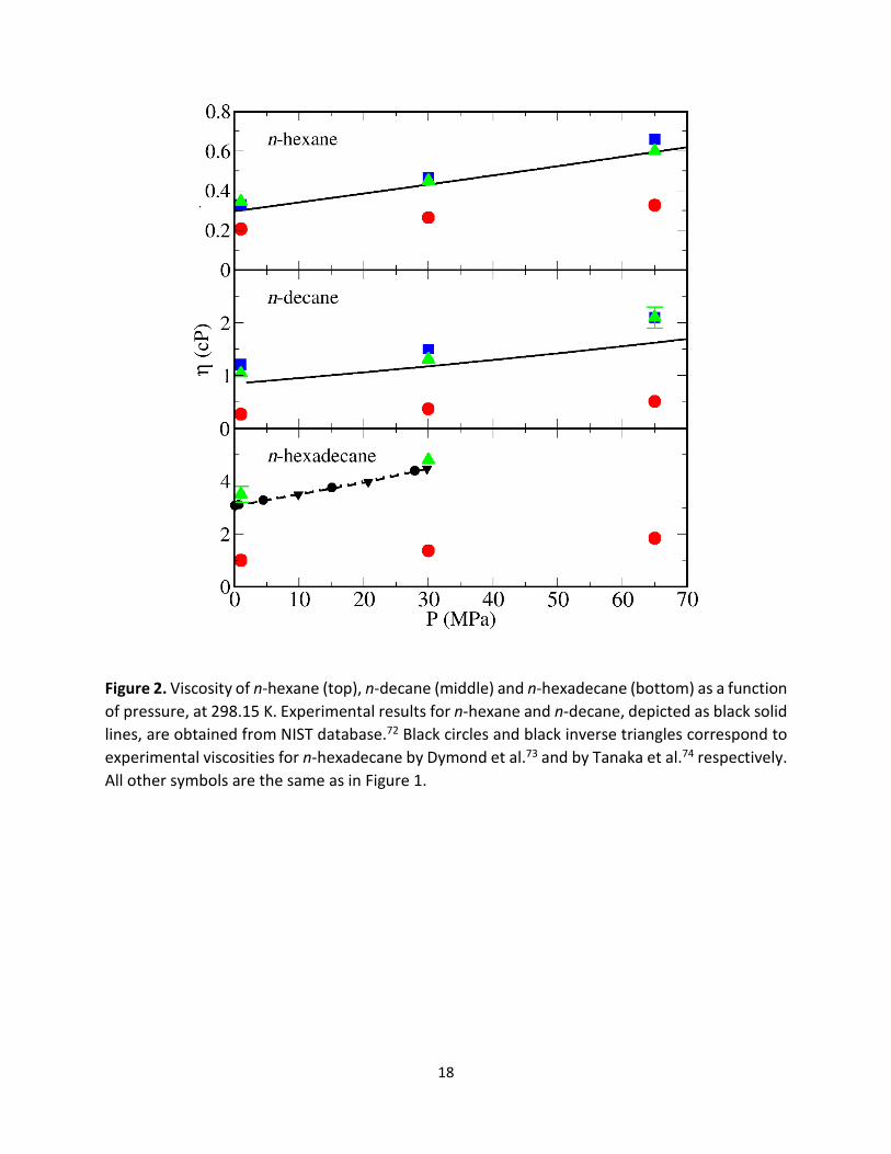
In an effort to obtain a better understanding of the accuracy of various force fields, we proceeded in performing density and viscosity calculations for the various systems and temperatures and pressures. These calculations are listed in Table 1. All force fields provide very accurate density predictions for the lower two temperatures (i.e., 298.15 and 323.15 K) with AADs lower or equal to 0.5%, while at 423.15 K the deviation is approximately 4%. While all force fields result in accurate density calculations, important deviations are observed for the viscosity values. In Figure 2 (top), MD calculations for the viscosity of n-hexane at 298.15 K are plotted as a function of pressure. OPLS-AA and L-OPLS models show very similar behavior, with L-OPLS being the most accurate (AAD of approx. 7.5%), while TraPPE-UA deviations from the experimental results are in the range of 16% – 38%. This deviation in viscosity can partially explain the poor performance of TraPPE-UA model for the prediction of diffusion coefficient of CO2 in n-hexane, and at the same time the small differences in OPLS-AA and L-OPLS. Similar behavior in viscosity can be seen also for the remaining of the n-alkanes examined (Figures 2 (middle) and 2 (bottom)) and temperatures considered (Table 1).
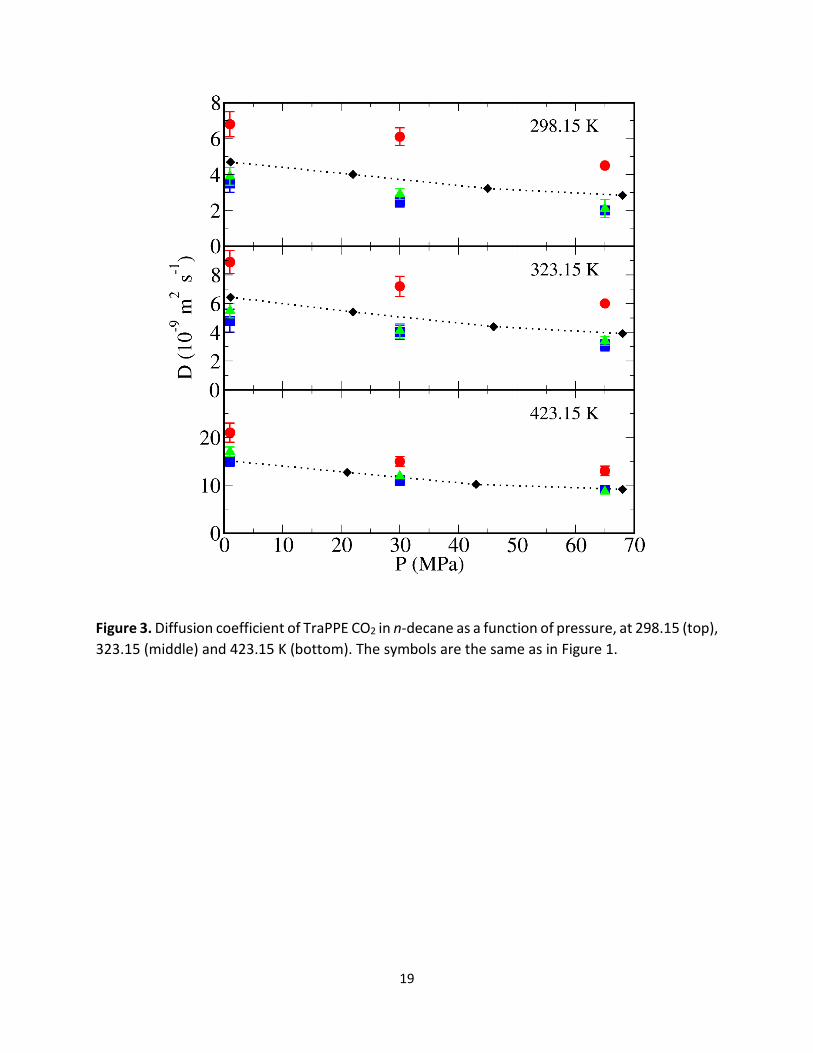
In Figure 3, the diffusion coefficient of CO2 in n-decane is plotted versus pressure at 298.15, 323.15 and 423.15 K. Although, the qualitative behavior of the different force fields is the same as in n-hexane systems, all of the models exhibit worse performance. In particular, TraPPE-UA overpredicts 𝐷𝐷𝐶𝐶𝐶𝐶2 by 28% – 64%, with an overall AAD approximately equal to 45%. The OPLS-AA and L-OPLS results are significantly more accurate than the TraPPE-UA, with AADs equal to 18% and 15%, respectively. It should be noted that for the highest simulated temperature of 423.15 K, the all-atom models give drastically improved 𝐷𝐷𝐶𝐶𝐶𝐶2, with OPLS-AA being the most accurate, deviating from experimental measurements by 0.5% – 6%. The density and viscosity calculations follow the same trends observed for the case of n-hexane. All models predict the density very accurately (i.e., approx. 1% deviation from the experimental values), while for the viscosity L-OPLS is the most accurate, and TraPPE is by far the least accurate. These results are in line with the work by Siu et al.36 who developed the L-OPLS force field.
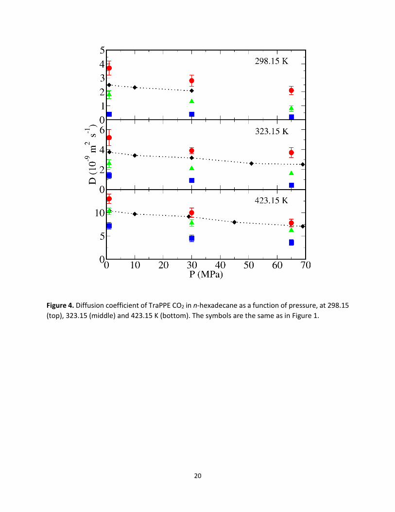
The MD results for 𝐷𝐷𝐶𝐶𝐶𝐶2 in n-hexadecane are summarized in Table 1 and depicted in Figure 4. For all temperatures and pressures studied, L-OPLS model exhibits the highest accuracy, as was for the cases of n-hexane and n-decane, discussed above. Additionally, the TraPPE-UA shows an
9
improved behavior in comparison with the n-decane, especially for 𝐷𝐷𝐶𝐶𝐶𝐶2 at 423.15 K. On the other hand, the OPLS-AA force field shows a significant underestimation of the diffusion coefficients at all temperatures and pressures examined, with the AAD ranging from 44% to 82%. Such a dramatic decrease in the quality of the OPLS-AA results can be primarily attributed to the poor density predictions by this model. In fact, Siu and co-workers36 developed the L-OPLS model motivated by similar observations for n-pentadecane. In their work they illustrated that OPLS-AA n-pentadecane predicts an overestimated melting temperature, 𝑇𝑇𝑚𝑚, resulting in unrealistic phase transitions. Siu et al.36 took into consideration the melting temperature of n-pentadecane into the optimization scheme and performed simulations in order to obtain more accurate gel-to-liquid transition temperatures for the optimized model. In order to achieve that, they modified the hydrogen charges and optimized the torsional potentials using ab initio gas phase calculations. Additionally, Siu et al. 36 achieved a significant improvement in predictions of gauche and trans fractions by modifying the interaction parameters of the methylene hydrogen atoms. As can be seen in Table 1, the liquid viscosities obtained by the L-OPLS force field are fairly accurate (AAD from experimental data of approx. 10%). In agreement with prior calculations by Siu et al. 36 for the case of n-pentadecane, our viscosity calculations for n-hexadecane with the OPLS-AA model at 298.15 K resulted in very high values (more than two orders of magnitude higher) indicating that the system is in a “gel-type” phase, and thus no calculations are reported for n-hexadecane using this force field. Siu et al.36 have shown that the original OPLS-AA torsional parameters predict this kind of phase transition for long alkanes even at temperatures well above the experimental 𝑇𝑇𝑚𝑚. In order to accurately predict the gel-to-liquid transition temperature for OPLS-AA n-hexadecane, a series of simulations at various temperatures is needed.
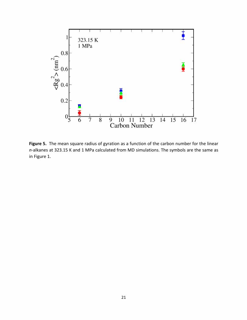
In an effort to explain further the differences between the various force fields, microscopic properties of the various systems were calculated. In Figure 5 the mean square radius of gyration, ⟨𝑅𝑅𝑎𝑎2⟩, of the n-alkanes is plotted against the carbon number for the three force fields studied at 323.15 K and 1 MPa. For all cases, TraPPE-UA predicts the lowest ⟨𝑅𝑅𝑎𝑎2⟩ followed by L-OPLS, while OPLS-AA shows the highest ⟨𝑅𝑅𝑎𝑎2⟩. In the case of n-hexadecane the difference becomes even more profound with OPLS-AA predicting an ⟨𝑅𝑅𝑎𝑎2⟩ almost 2 times higher than the rest of the models. Given that OPLS-AA and L-OPLS models have relatively similar values for the LJ parameters, this difference in ⟨𝑅𝑅𝑎𝑎2⟩ can be attributed to the optimized torsional potentials of L-OPLS. This fact can partially explain why the specific solvent force field predicts the lowest viscosity and, consequently, the lowest 𝐷𝐷𝐶𝐶𝐶𝐶2.
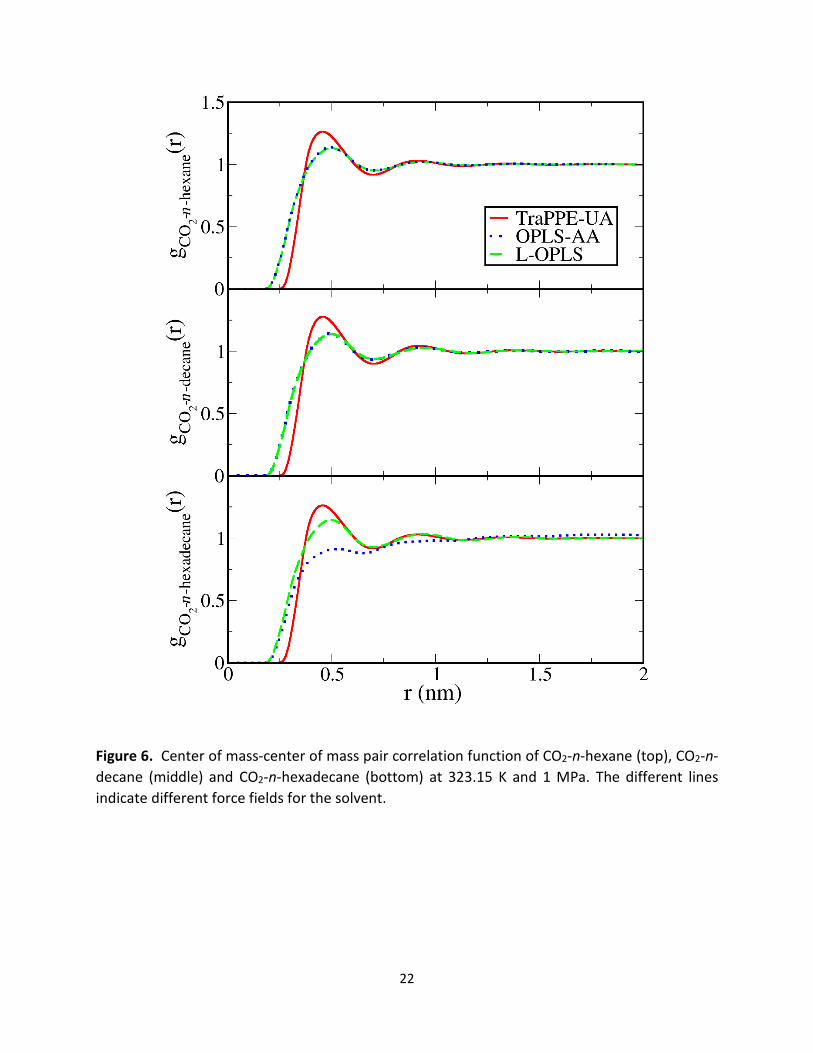
The center of mass pair correlation function, g(r), for CO2 – n-alkane interactions was calculated for CO2 – n-hexane, CO2 – n-decane and CO2 – n-hexadecane at 323.15 K and 1 MPa in order to further understand the microscopic differences between the three force fields. Results are shown in Figure 6. Clearly, TraPPE predicts a much stronger CO2 – n-alkane interactions while the two variations of OPLS differentiate only at the longest n-alkane examined.
10
The combination of different chain sizes and solute – solvent interactions predicted by the three models result in different macroscopic property predictions (viscosity and diffusion coefficient).
3.2 Diffusion coefficients of CO2 in cyclohexane and squalane. MD simulations were performed for the calculation of diffusion coefficients of CO2 in a cyclic and a branched hydrocarbon, namely cyclohexane and squalane, and the results are compared to the experimental measurements by Cadogan et al.15 and Cadogan.16 The force fields used for the representation of the hydrocarbons were TraPPE-UA and OPLS-AA. No simulations were performed using L-OPLS since there are no parameters currently available in this force field for cyclic or branched molecules. All MD results are listed in Table 2.
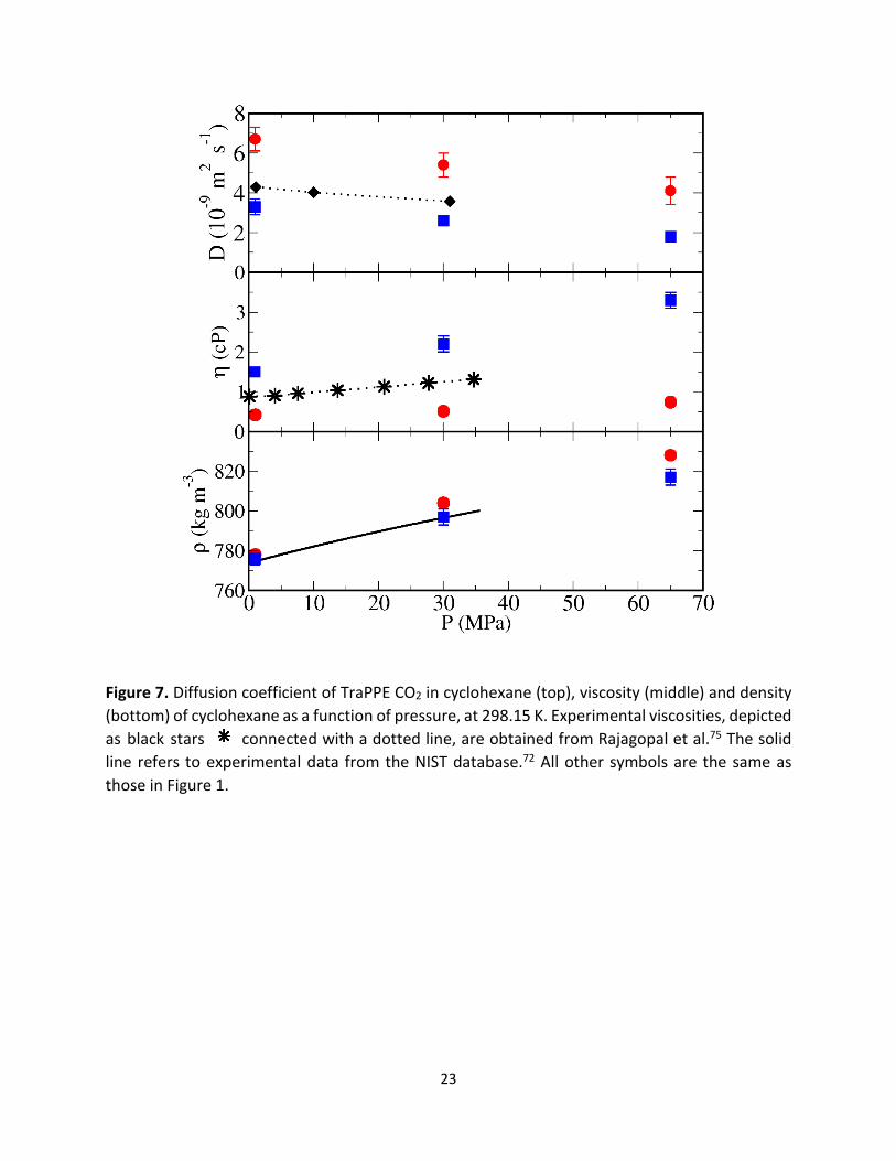
In Figure 7, the diffusion coefficient of CO2 in cyclohexane (top) is plotted as a function of pressure at 298.15 K. The simulations with TraPPE-UA result in overestimating 𝐷𝐷𝐶𝐶𝐶𝐶2 by approximately 54%, while the use of OPLS-AA model, although giving improved predictions, results in underestimating diffusivities by 25%, at the specific temperature and pressures up to 30 MPa. In Figure 7 (middle), the viscosity of cyclohexane is plotted for the two models. Consistently to the simulations for linear alkanes, TraPPE-UA underestimates viscosity by almost a factor of 2, while OPLS-AA overshoots viscosity by approximately 68%. However, both force fields predict liquid densities very accurately (AAD of approx. 1%) as can be seen in Figure 7 (bottom). The failure of both models in predicting accurately the viscosity of cyclohexane can partly explain the inaccurate results for diffusion coefficients.
Similar conclusions can be drawn for calculations at 323.15 and 423.15 K, shown in Table 2. As temperature increases, 𝐷𝐷𝐶𝐶𝐶𝐶2 predictions improve for both force fields. At 423.15 K, TraPPE-UA overestimates diffusivity by approximately 20%, while OPLS-AA underestimates it by 13%, compared to the experiments by Cadogan.16 This improvement, again, can be attributed to the improved viscosity predictions by both models. TraPPE-UA deviates from experimental viscosity data65 by 22% and OPLS-AA by 4%.
Simulations for squalane revealed a similar behavior for the various molecular models, as discussed up to this point. TraPPE-UA performs poorly for the prediction of 𝐷𝐷𝐶𝐶𝐶𝐶2, having an average deviation from experiments, over all conditions, approximately equal to 76%. The respective AAD for OPLS-AA is 41%. Both models give improved results at the highest temperature, 423.15 K, with TraPPE overestimating diffusivity of CO2 in squalane by 30% and OPLS-AA by 22%. No viscosities were obtained for squalane, due to the very computational–demanding simulations, however similar behavior with the rest of the hydrocarbons studied is expected. Both models, predict density very accurately (AAD of approx. 1%).
Overall, there is a strong dependence of 𝐷𝐷𝐶𝐶𝐶𝐶2 on the solvent’s molecular size because the motion of CO2 molecules is hindered by molecules with higher carbon number, as expected. Our MD simulations were long enough so that CO2 molecules travel several times longer than the average size of a solvent molecule. For example, at 323.15 K and 1 MPa the ⟨𝑅𝑅𝑎𝑎2⟩1/2 of n-hexane
11
using TraPPE-UA is equal to 0.21 nm while the total average displacement of the CO2 molecules after 10 ns is approximately 7 nm. Furthermore, ⟨𝑅𝑅𝑎𝑎2⟩1/2 for squalane using TraPPE is equal to 0.83 nm while the displacement of CO2 after 10 ns is 4.1 nm. Similar results are obtained for all the systems and temperature/pressure conditions examined.
3.3 Stokes-Einstein analysis. The translational motion of a solute in a fluid solution at infinite dilution can be described by the Einstein equation:19-20
𝐷𝐷 =𝑘𝑘𝐵𝐵𝑇𝑇𝜁𝜁
(11)
where D is the diffusion coefficient, kB is the Boltzmann’s constant, T is the absolute temperature and 𝜁𝜁 is the friction coefficient. At the hydrodynamic limit of a sphere of radius, 𝑟𝑟, diffusing in a fluid having a shear viscosity, 𝜂𝜂, one can recover the Stokes-Einstein (SE) relation
𝐷𝐷 =𝑘𝑘𝐵𝐵𝑇𝑇𝐶𝐶𝜋𝜋𝜂𝜂𝑟𝑟
(12)
where the constant C is determined by the boundary conditions and is equal to 4 or 6 for the case of “slip” or “stick” boundary conditions respectively. Equation 12 was originally developed for cases when the size of the diffusing solute is much larger than the size of the solvent. Nevertheless, it has been also found that the SE relation provides good results for cases that the diffusing object is a molecule of the same liquid (i.e., self-diffusion). Such an example is the case of the experimental measurements reported by Xu et al.66 who confirmed the validity of the SE relation for the self-diffusion coefficients of water at temperatures higher than approximately 290 K. On the other hand, experimental studies have reported deviations for cases when the size of the solute is smaller or comparable to the size of the solvent. Some typical examples include the study of Pollack and Enyeart67 who reported experimental measurements of 133Xe in n-alkanes. Similarly, Kowert and Dang68 performed experiments of O2 in n-alkanes.
One approach to account for the deviation from SE relation is to consider the solute radius, r, as a variable to be fitted to experimental measurements.69-70 In other words, r is treated as an “effective hydrodynamic radius”. Such an approach was also considered in the recent experimental study of Cadogan et al.15
An alternative approach is to use the fractional Stokes-Einstein (FSE) relation,71 usually expressed as:
𝐷𝐷𝑇𝑇∝ �
1𝜂𝜂�𝑡𝑡
(13)
Or:
𝐷𝐷 ∝ �𝑇𝑇𝜂𝜂�𝑡𝑡
(14)
12
where the exponents t and s have values different from 1 for the case of FSE, and equal to 1 for the case of SE.
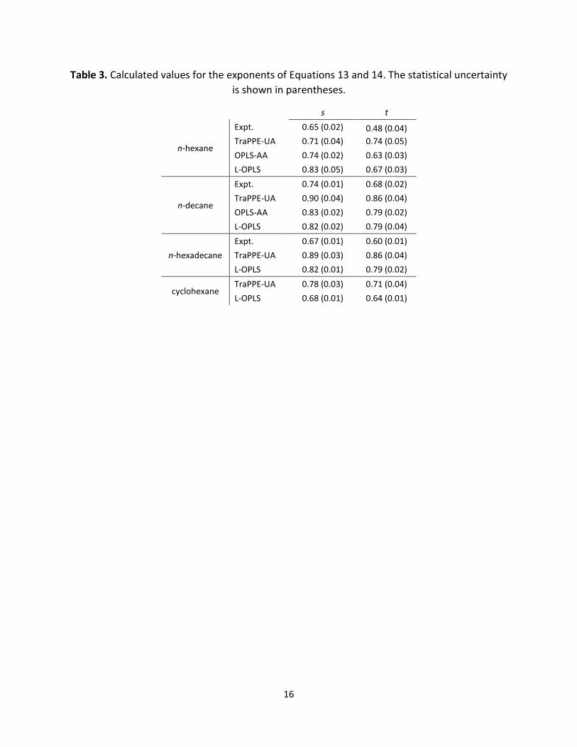
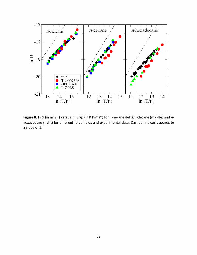
In the current study, we focus on the second approach. The exponents corresponding to different models used in the MD simulations are calculated from the slope of double logarithmic plots. A characteristic example is shown in Figure 8 where the logarithm of 𝐷𝐷𝐶𝐶𝐶𝐶2 is plotted as a function of ln(𝑇𝑇 𝜂𝜂⁄ ), for the linear alkanes examined. In addition, lines with a slope equal to s=1 (corresponding to SE) are also shown. Deviations from the SE limit are clearly observed in all cases. In Table 3 the calculated exponents for all the hydrocarbons examined are listed, except for squalane for which no viscosity simulations were performed. The deviation from Stokes-Einstein behavior, observed for the MD data, is in line with the experimental results by Cadogan et al., also shown in Figure 8 and Table 3.
4. Conclusions Atomistic MD simulations of the diffusion coefficients of infinitely diluted CO2 in n-hexane, n-decane, n-hexadecane, cyclohexane and squalane were performed at 298.15, 323.15 and 423.15 K for pressures up to 65 MPa. A comprehensive evaluation of three widely used molecular models for hydrocarbons, namely the TraPPE-UA, OPLS-AA and L-OPLS, were performed by comparing simulation results with the recently reported experimental measurements by Cadogan et al.
Overall the TraPPE-UA model, although computationally efficient due to the united atom representation and the absence of electrostatic contributions, was found to be on the average the least accurate for all hydrocarbons examined (with the exception of n-hexadecane), while L-OPLS, an optimized form of OPLS-AA model, yielded the best results for the case of n-alkanes. More specifically, L-OPLS, having optimized torsional potentials and charges, was able to reproduce liquid density and viscosity more accurately compared to the original OPLS-AA, which showed an early gel-to-liquid transition and thus was unable to be used for the present study for the case of n-hexadecane. In addition, simulation results succeeded in qualitatively reproducing the pressure dependence of 𝐷𝐷𝐶𝐶𝐶𝐶2, shown in the experiments. Microscopic properties such as the mean square radius of gyration for the n-alkanes and the pair correlation function between CO2 and n-alkane molecules were shown to be different from the different force fields and result in different macroscopic property predictions.
The diffusion coefficients of CO2 in all alkanes examined, and with all force fields employed, were shown to deviate significantly from the Stokes-Einstein behavior. These results are in agreement with the experimental measurements, which exhibited also fractional Stokes-Einstein behavior. Finally, the diffusion coefficient values correlate reasonably well (linear behavior) with the molar volume of the hydrocarbon for each system examined. Details for these calculations are provided in the Supporting Information.
13
Supporting information The supporting information file contains tables with the following information: parameters for OPLS-AA, L-OPLS and TraPPE-UA force fields for hydrocarbons, and TraPPE-UA force field for CO2, composition and box size lengths for the various simulations performed. It also contains figures with diffusion coefficients of CO2 in hydrocarbons, percentage average absolute deviations between experimental data and molecular simulations for the diffusion coefficient of CO2 in hydrocarbons, viscosity and density of various hydrocarbons and of DT0.5 of CO2 in n-alkanes vs. the molar volume of the corresponding n-alkane.
Acknowledgments This publication was made possible by NPRP [grant number 6-1157-2-471] form the Qatar
National Research Fund (a member of Qatar Foundation). The statements made herein are solely the responsibility of the authors. We are grateful to the High Performance Computing Center of Texas A&M University at Qatar for generous resource allocation. Additionally, we would like to thank Professor A. Böckman and his group for useful discussions on the implementation of the L-OPLS force field.
14
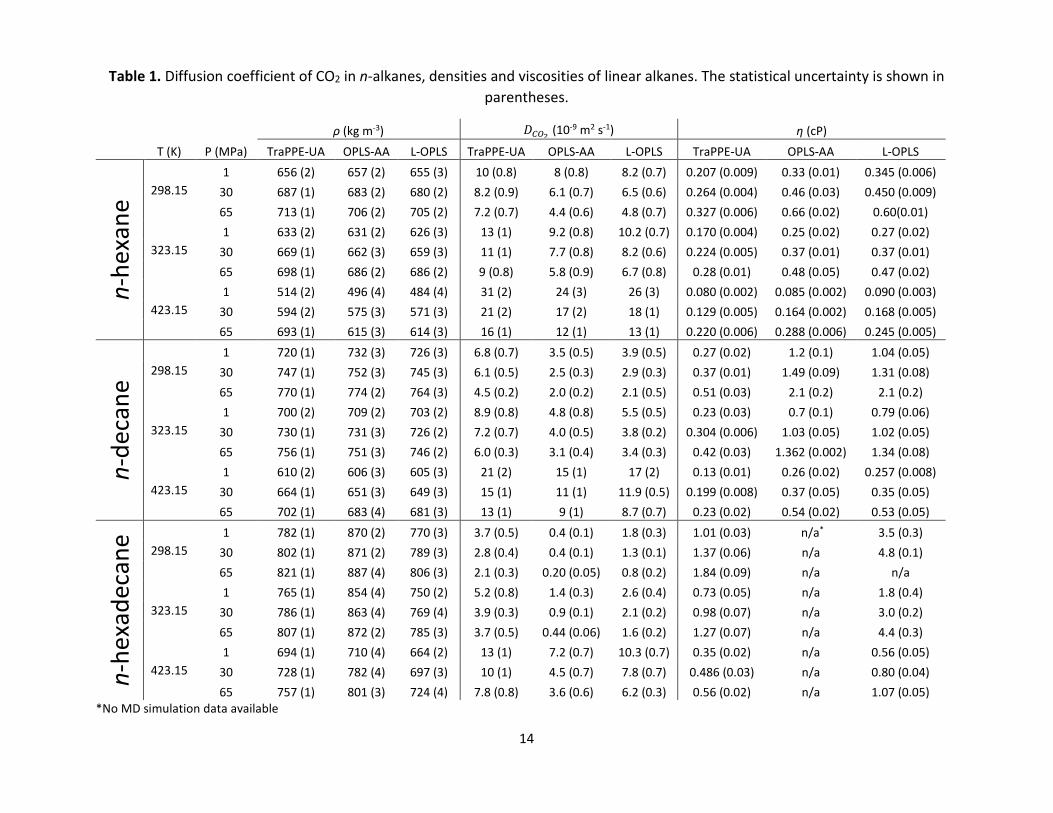
Table 1. Diffusion coefficient of CO2 in n-alkanes, densities and viscosities of linear alkanes. The statistical uncertainty is shown in parentheses.
ρ (kg m-3) 𝐷𝐷𝐶𝐶𝐶𝐶2 (10-9 m2 s-1) η (cP)
T (K) P (MPa) TraPPE-UA OPLS-AA L-OPLS TraPPE-UA OPLS-AA L-OPLS TraPPE-UA OPLS-AA L-OPLS
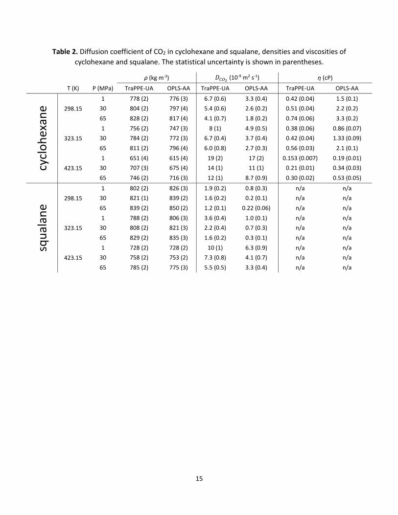
Table 2. Diffusion coefficient of CO2 in cyclohexane and squalane, densities and viscosities of cyclohexane and squalane. The statistical uncertainty is shown in parentheses.
ρ (kg m-3) 𝐷𝐷𝐶𝐶𝐶𝐶2 (10-9 m2 s-1) η (cP)
T (K) P (MPa) TraPPE-UA OPLS-AA TraPPE-UA OPLS-AA TraPPE-UA OPLS-AA
Figure 1. Diffusion coefficient of TraPPE CO2 in n-hexane as a function of pressure, at 298.15 (top), 323.15 (middle) and 423.15 K (bottom). Black diamonds connected with dotted lines correspond to experimental measurements by Cadogan et al.15 and Cadogan.16 Colored symbols correspond to different force fields for n-hexane: red circles correspond to TraPPE-UA, blue squares to OPLS-AA and green triangles to L-OPLS. Error bars smaller than the plotting symbol are omitted.
18
Figure 2. Viscosity of n-hexane (top), n-decane (middle) and n-hexadecane (bottom) as a function of pressure, at 298.15 K. Experimental results for n-hexane and n-decane, depicted as black solid lines, are obtained from NIST database.72 Black circles and black inverse triangles correspond to experimental viscosities for n-hexadecane by Dymond et al.73 and by Tanaka et al.74 respectively. All other symbols are the same as in Figure 1.
19
Figure 3. Diffusion coefficient of TraPPE CO2 in n-decane as a function of pressure, at 298.15 (top), 323.15 (middle) and 423.15 K (bottom). The symbols are the same as in Figure 1.
20
Figure 4. Diffusion coefficient of TraPPE CO2 in n-hexadecane as a function of pressure, at 298.15 (top), 323.15 (middle) and 423.15 K (bottom). The symbols are the same as in Figure 1.
21
Figure 5. The mean square radius of gyration as a function of the carbon number for the linear n-alkanes at 323.15 K and 1 MPa calculated from MD simulations. The symbols are the same as in Figure 1.
22
Figure 6. Center of mass-center of mass pair correlation function of CO2-n-hexane (top), CO2-n-decane (middle) and CO2-n-hexadecane (bottom) at 323.15 K and 1 MPa. The different lines indicate different force fields for the solvent.
23
Figure 7. Diffusion coefficient of TraPPE CO2 in cyclohexane (top), viscosity (middle) and density (bottom) of cyclohexane as a function of pressure, at 298.15 K. Experimental viscosities, depicted as black stars connected with a dotted line, are obtained from Rajagopal et al.75 The solid line refers to experimental data from the NIST database.72 All other symbols are the same as those in Figure 1.
24
Figure 8. ln D (in m2 s-1) versus ln (T/η) (in K Pa-1 s-1) for n-hexane (left), n-decane (middle) and n-hexadecane (right) for different force fields and experimental data. Dashed line corresponds to a slope of 1.
25
References
1. Lake, L. W., Enhanced Oil Recovery; Prentice Hall: Old Tappan, NJ, 1989. 2. Metz, B.; Davidson, O.; de Coninck, H.; Loos, M.; Meyer, L., Carbon Dioxide Capture and Storage: Special Report of the Intergovernmental Panel on Climate Change; Cambridge University Press: Cambridge, 2005. 3. Hayduk, W.; Cheng, S. C. Review of relation between diffusivity and solvent viscosity in dilute liquid solutions. Chem. Eng. Sci. 1971, 26, 635–646. 4. Takeuchi, H.; Fujine, M.; Sato, T.; Onda, K. Simultaneous determination of diffusion coefficient and solubility of gas in liquid by a diaphragm cell. J. Chem. Eng. Jpn. 1975, 8, 252–253. 5. Matthews, M. A.; Rodden, J. B.; Akgerman, A. A. High-temperature diffusion of hydrogen, carbon monoxide, and carbon dioxide in liquid n-heptane, n-dodecane, and n-hexadecane. J. Chem. Eng. Data 1987, 32, 319–322. 6. Grogan, A. T.; Pinczewski, W. V. The role of molecular diffusion processes in tertiary CO2 flooding. J. Petrol. Technol. 1987, 39, 591–602. 7. Grogan, A.; Pinczewski, W. V.; Ruskauff, G.; Orr, F. M. Diffusion of CO2 at reservoir conditions: models and measurements. SPE Reserv. Eng. 1988, 3, 93–102. 8. Luthjens, L. H.; de Leng, H. C.; Warman, J. M.; Hummel, A. Diffusion coefficients of gaseous scavengers in organic liquids used in radiation chemistry. International Journal of Radiation Applications and Instrumentation. Part C. Radiation Physics and Chemistry 1990, 36, 779–784. 9. Guzmán, J.; Garrido, L. Determination of carbon dioxide transport coefficients in liquids and polymers by NMR spectroscopy. J. Phys. Chem. B 2012, 116, 6050–6058. 10. Teng, Y. L., Y.; Song, Y.; Jiang, L.; Zhao, Y.; Zhou, X.; Zheng, H.; Chen, J. A study on CO2 diffusion coefficient in n-decane saturated porous media by MRI. Energy Procedia 2014, 61, 603–606. 11. Hao, M.; Song, Y. C.; Su, B.; Zhao, Y. C. Diffusion of CO2 in n-hexadecane determined from NMR relaxometry measurements. Phys. Lett. A 2015, 379, 1197–1201. 12. Nikkhou, F.; Keshavarz, P.; Ayatollahi, S.; Zolghadr, A. Interfacial resistance in CO2-normal alkane and N2-normal alkane systems: An experimental and modeling investigation. Korean J. Chem. Eng. 2015, 32, 222–229. 13. Nikkhou, F.; Keshavarz, P.; Ayatollahi, S.; Jahromi, I. R.; Zolghadr, A. Evaluation of interfacial mass transfer coefficient as a function of temperature and pressure in carbon dioxide/normal alkane systems. Heat Mass Transfer. 2014, 51, 477–485. 14. Liu, Y.; Teng, Y.; Lu, G.; Jiang, L.; Zhao, J.; Zhang, Y.; Song, Y. Experimental study on CO2 diffusion in bulk n-decane and n-decane saturated porous media using micro-CT. Fluid Phase Equilib. 2016, 417, 212–219. 15. Cadogan, S. P.; Mistry, B.; Wong, Y.; Maitland, G. C.; Trusler, J. P. M. Diffusion coefficients of carbon dioxide in eight hydrocarbon liquids at temperatures between (298.15 and 423.15) K at pressures up to 69 MPa. J. Chem. Eng. Data. 2016, 61, 3922-3932. 16. Cadogan, S. P. Diffusion of CO2 in Fluids Relevant to Carbon Capture, Utilisation and Storage, Ph.D. Thesis, Imperial College, London, 2015. 17. Bird, R. B.; Klingenberg, D. J. Multicomponent diffusion-A brief review. Adv. Water Res. 2013, 62, 238–242. 18. Brokaw, R. S. Predicting transport properties of dilute gases. Ind. Eng. Chem. Process. Des. Dev. 1969, 8, 240–253. 19. Cussler, E. L., Diffusion: Mass Transfer in Fluid Systems, 3rd ed.; Cambridge University Press: Cambridge, 2009. 20. Tyrrell, H. J. V.; Harris, K. R., Diffusion in Liquids. A Theoretical and Experimental Study.; Butterworths: London, 1984.
26
21. Tyrrell, Z. L.; Shen, Y. Q.; Radosz, M. Fabrication of micellar nanoparticles for drug delivery through the self-assembly of block copolymers. Prog. Polym. Sci. 2010, 35, 1128–1143. 22. Allen, M. P.; Tildesley, D. J., Computer Simulation of Liquids: Oxford University Press, 1987. 23. Harris, J. G.; Yung, K. H. Carbon dioxide's liquid-vapor coexistence curve and critical properties as predicted by a simple molecular model. J. Phys. Chem. 1995, 99, 12021–12025. 24. Potoff, J. J.; Siepmann, J. I. Vapor-liquid equilibria of mixtures containing alkanes, carbon dioxide, and nitrogen. AIChE J. 2001, 47, 1676–1682. 25. Jiang, H.; Moultos, O. A.; Economou, I. G.; Panagiotopoulos, A. Z. Gaussian-charge polarizable and nonpolarizable models for CO2. J. Phys. Chem. B 2016, 120, 984–994. 26. Moultos, O. A.; Tsimpanogiannis, I. N.; Panagiotopoulos, A. Z.; Economou, I. G. Self-diffusion coefficients of the binary (H2O + CO2) mixture at high temperatures and pressures. J. Chem. Thermodyn. 2016, 93, 424–429. 27. Moultos, O. A.; Tsimpanogiannis, I. N.; Panagiotopoulos, A. Z.; Economou, I. G. Atomistic molecular dynamics simulations of CO2 diffusivity in H2O for a wide range of temperatures and pressures. J. Phys. Chem. B 2014, 118, 5532–5541. 28. Moultos, O. A.; Orozco, G. A.; Tsimpanogiannis, I. N.; Panagiotopoulos, A. Z.; Economou, I. G. Atomistic molecular dynamics simulations of H2O diffusivity in liquid and supercritical CO2. Mol. Phys. 2015, 113, 2805–2814. 29. Jorgensen, W. L.; Maxwell, D. S.; Tirado-Rives, J. Development and testing of the OPLS all-atom force field on conformational energetics and properties of organic liquids. J. Am. Chem. Soc. 1996, 118, 11225–11236. 30. Price, M. L. P.; Ostrovsky, D.; Jorgensen, W. L. Gas-phase and liquid-state properties of esters, nitriles, and nitro compounds with the OPLS-AA force field. J. Comput. Chem. 2001, 22, 1340–1352. 31. Jorgensen, W. L.; Madura, J. D.; Swenson, C. J. Optimized intermolecular potential functions for liquid hydrocarbons. J. Am. Chem. Soc. 1984, 106, 6638–6646. 32. Jorgensen, W. L.; Tirado-Rives, J. The OPLS potential functions for proteins. Energy minimizations for crystals of cyclic peptides and crambin. J. Am. Chem. Soc. 1988, 110, 1657–1666. 33. Martin, M. G.; Siepmann, J. I. Transferable potentials for phase equilibria. 1. United-atom description of n-alkanes. J. Phys. Chem. B 1998, 102, 2569–2577. 34. Chen, B.; Siepmann, J. I. Transferable potentials for phase equilibria. 3. Explicit-hydrogen description of normal alkanes. J. Phys. Chem. B 1999, 103, 5370–5379. 35. Weiner, S. J.; Kollman, P. A.; Nguyen, D. T.; Case, D. A. An all atom force field for simulations of proteins and nucleic acids. J. Comput. Chem. 1986, 7, 230–252. 36. Siu, S. W. I.; Pluhackova, K.; Böckmann, R. A. Optimization of the OPLS-AA force field for long hydrocarbons. J. Chem. Theory Comput. 2012, 8, 1459–1470. 37. Paul, W.; Yoon, D. Y.; Smith, G. D. An optimized united atom model for simulations of polymethylene melts. J. Chem. Phys. 1995, 103, 1702–1709. 38. Ungerer, P.; Beauvais, C.; Delhommelle, J.; Boutin, A.; Rousseau, B.; Fuchs, A. H. Optimization of the anisotropic united atoms intermolecular potential for n-alkanes. J. Chem. Phys. 2000, 112, 5499–5510. 39. Li, H. P.; Maroncelli, M. Solvation and solvatochromism in CO2-expanded liquids. 1. Simulations of the solvent systems CO2 + cyclohexane, acetonitrile, and methanol. J. Phys. Chem. B 2006, 110, 21189–21197. 40. Zabala, D.; Nieto-Draghi, C.; de Hemptinne, J. C.; López de Ramos, A. L. Diffusion coefficient in CO2/n-alkane binary liquid mixture by molecular simulation. J. Phys. Chem. B 2008, 112, 16610–16618. 41. Makrodimitri, Z. A.; Unruh, D. J. M.; Economou, I. G. Molecular simulation of diffusion of hydrogen, carbon monoxide, and water in heavy n-alkanes. J. Phys. Chem. B 2011, 115, 1429–1439.
27
42. Van der Ploeg, P.; Berendsen, H. J. C. Molecular dynamics simulation of a bilayer membrane. J. Chem. Phys. 1982, 76, 3271–3276. 43. Ryckaert, J. P.; Bellemans, A. Molecular dynamics of liquid alkanes. Faraday Discuss. Chem. Soc. 1978, 66, 95–106. 44. Ryckaert, J. P.; Ciccotti, G.; Berendsen, H. J. C. Numerical integration of the Cartesian equations of motion of a system with constraints: molecular dynamics of n-alkanes. J. Comput. Phys. 1977, 23, 327–341. 45. Potoff, J. J.; Errington, J. R.; Panagiotopoulos, A. Z. Molecular simulation of phase equilibria for mixtures of polar and non-polar components. Mol. Phys. 1999, 97, 1073–1083. 46. Nezbeda, I.; Moučka, F.; Smith, W. R. Recent progress in molecular simulation of aqueous electrolytes: force fields, chemical potentials and solubility. Mol. Phys. 2016, 114, 1665–1690. 47. Desgranges, C.; Delhommelle, J. Evaluation of the grand-canonical partition function using expanded Wang-Landau simulations. III. Impact of combining rules on mixtures properties. J. Chem. Phys. 2014, 140, 104109. 48. Soetens, J.-C.; Bopp, P. A. Water-Methanol Mixtures: Simulations of Mixing Properties over the Entire Range of Mole Fractions. J. Phys. Chem. B 2015, 119, 8593–8599. 49. Berendsen, H. J. C.; van der Spoel, D.; van Drunen, R. GROMACS: A message-passing parallel molecular dynamics implementation. Comput. Phys. Commun. 1995, 91, 43–56. 50. Lindahl, E.; Hess, B.; van der Spoel, D. GROMACS 3.0: A package for molecular simulation and trajectory analysis. J. Mol. Model. 2001, 7, 306–317. 51. Darden, T.; York, D.; Pedersen, L. Particle mesh Ewald: An N·log(N) method for Ewald sums in large systems. J. Chem. Phys. 1993, 98, 10089–10092. 52. Essmann, U.; Perera, L.; Berkowitz, M. L.; Darden, T.; Lee, H.; Pedersen, L. G. A smooth particle mesh Ewald method. J. Chem. Phys. 1995, 103, 8577–8593. 53. Nosé, S. A molecular dynamics method for simulations in the canonical ensemble. Mol. Phys. 1984, 52, 255–268. 54. Hoover, W. G. Canonical dynamics: Equilibrium phase-space distributions. Phys. Rev. A 1985, 31, 1695–1697. 55. Parrinello, M.; Rahman, A. Polymorphic transitions in single crystals: A new molecular dynamics method. J. Appl. Phys. 1981, 52, 7182–7190. 56. Bussi, G.; Donadio, D.; Parrinello, M. Canonical sampling through velocity rescaling. J. Chem. Phys. 2007, 126, 014101. 57. van der Spoel, D.; van Maaren, P. J. The origin of layer structure artifacts in simulations of liquid water. J. Chem. Theory Comput. 2006, 2, 1–11. 58. Einstein, A. Über die von der molekularkinetischen Theorie der Wärme geforderte Bewegung von in ruhenden Flüssigkeiten suspendierten Teilchen. Ann. Phys. 1905, 17, 549–560. 59. Sadus, R. J., Molecular Simulation of Fluids: Theory, Algorithms and Object-Orientation, Elsevier, Amsterdam, 1999. 60. Yeh, I. C.; Hummer, G. System-size dependence of diffusion coefficients and viscosities from molecular dynamics simulations with periodic boundary conditions. J. Phys. Chem. B 2004, 108, 15873–15879. 61. Cadogan, S. P.; Maitland, G. C.; Trusler, J. P. M. Diffusion coefficients of CO2 and N2 in water at temperatures between 298.15 K and 423.15 K at pressures up to 45 MPa. J. Chem. Eng. Data 2014, 59, 519–525. 62. Mondello, M.; Grest, G. S. Viscosity calculations of n-alkanes by equilibrium molecular dynamics. J. Chem. Phys. 1997, 106, 9327–9336. 63. Mondello, M.; Grest, G. S.; Webb, E. B.; Peczak, P. Dynamics of n-alkanes: Comparison to Rouse model. J. Chem. Phys. 1998, 109, 798–805.
28
64. Mondello, M.; Grest, G. S. Molecular dynamics of linear and branched alkanes. J. Chem. Phys. 1995, 103, 7156–7165. 65. Liu, Z.; Trusler, J. P. M.; Bi, Q. Viscosities of liquid cyclohexane and decane at temperatures between (303 and 598) K and pressures up to 4 MPa measured in a dual-capillary viscometer. J. Chem. Eng. Data 2015, 60, 2363–2370. 66. Xu, L.; Mallamace, F.; Yan, Z.; Starr, F.W.; Buldyrev, S.V.; Stanley, E. H. Appearance of a fractional Stokes-Einstein relation in water and a structural interpretation of its onset. Nature Physics 2009, 5, 565–569. 67. Pollack, G. L.; Enyeart, J. J. Atomic test of the Stokes-Einstein law. II. Diffusion of Xe through liquid hydrocarbons. Phys. Rev. A 1985, 31, 980–984. 68. Kowert, B. A.; Dang, N. C., Diffusion of dioxygen in n-alkanes. J. Phys. Chem. A 1999, 103, 779–781. 69. Zwanzig, R.; Harrison, A. K. Modifications of the Stokes-Einstein formula. J. Chem. Phys. 1985, 83, 5861–5862. 70. Kowert, B.; Sobush, K.; Fuqua, C.; Mapes, C.; Jones, J.; Zahm, J. Size-dependent diffusion in the n-alkanes. J. Phys. Chem. A 2003, 107, 4790–4795. 71. Harris, K. R. The fractional Stokes-Einstein equation: Application to Lennard-Jones, molecular, and ionic liquids. J. Chem. Phys. 2009, 131, 054503. 72. Lemmon, E. W.; McLinden, M. O.; Friend, D. G.; Linstrom, P. J.; Mallard, W. G., NIST Chemistry Webbook, 2014. 73. Dymond, J. H.; Young, K. J.; Isdale, J. D. Transport properties of nonelectrolyte liquid mixtures-II. Viscosity coefficients for the n-hexane + n-hexadecane system at temperatures from 25 to 100 oC at pressures up to the freezing pressure or 500 MPa. Int. J. Thermophys. 1980, 1, 345–373. 74. Tanaka, Y.; Hosokawa, H.; Kubota, H.; Makita, T. Viscosity and density of binary mixtures of cyclohexane with n-octane, n-dodecane, and n-hexadecane under high pressures. Int. J. Thermophys. 1991, 12, 245–264. 75. Rajagopal, K.; Andrade, L. L. P. R.; Paredes, M. L. L. High-pressure viscosity measurements for the binary system cyclohexane + n-hexadecane in the temperature range of (318.15 to 413.15) K. J. Chem. Eng. Data 2009, 54, 2967–2970. 76. Moultos, O. A.; Zhang, Y.; Tsimpanogiannis, I. N.; Economou, I. G.; Maginn, E. M. System-size corrections for self-diffusion coefficients calculated from molecular dynamics simulations: The case of CO2, n-alkanes, and poly(ethylene glycol) dimethyl ethers. J. Chem. Phys. 2016, 145, 074109.


![312-01 pres-e LIPOGARD [Schreibgeschützt] presentation.pdf · LIPOGARD activity The well balanced mixture of Q10 and Vitamin E offers in a squalane based formula unique activities:](https://static.documents.pub/doc/80x56/5a72dc8b7f8b9aa2538e1a8c/312-01-pres-e-lipogard-schreibgeschuetzt-presentationpdf-lipogard-activity.jpg)