N O T A C N Information Retrieval on Noisy Text

I

CO

MM

UN

CA

TI

ON

ID

IA

P

Rue du Simplon 4

IDIAP Research Institute1920 Martigny − Switzerland

www.idiap.ch

Tel: +41 27 721 77 11 Email: [email protected]. Box 592Fax: +41 27 721 77 12

Information Retrieval onNoisy Text

David Grangier 1,2 Alessandro Vinciarelli 1

Herve Bourlard 1

IDIAP–Com 03-08

- 32 -

1 IDIAP, Martigny, Switzerland2 Eurecom, Sophia-Antipolis, France

Contents

1 Introduction 3

2 State of the Art 52.1 Introduction . . . . . . . . . . . . . . . . . . . . . . . . . . . . . . . . . . . . . . . . . . 52.2 Structure of an SDR System . . . . . . . . . . . . . . . . . . . . . . . . . . . . . . . . . 5

2.2.1 Speech Recognition . . . . . . . . . . . . . . . . . . . . . . . . . . . . . . . . . . 62.2.2 Segmentation . . . . . . . . . . . . . . . . . . . . . . . . . . . . . . . . . . . . . 72.2.3 Preprocessing and Normalization . . . . . . . . . . . . . . . . . . . . . . . . . . 72.2.4 Indexing . . . . . . . . . . . . . . . . . . . . . . . . . . . . . . . . . . . . . . . . 8

2.2.4.1 The Binary Model . . . . . . . . . . . . . . . . . . . . . . . . . . . . . 92.2.4.2 The Vector Space Model . . . . . . . . . . . . . . . . . . . . . . . . . 92.2.4.3 The Probabilistic Model . . . . . . . . . . . . . . . . . . . . . . . . . . 10

2.2.5 Retrieval . . . . . . . . . . . . . . . . . . . . . . . . . . . . . . . . . . . . . . . 102.2.5.1 Preprocessing, Normalization and Indexing . . . . . . . . . . . . . . . 112.2.5.2 Query Expansion . . . . . . . . . . . . . . . . . . . . . . . . . . . . . 112.2.5.3 Matching Measures and Ranking . . . . . . . . . . . . . . . . . . . . . 142.2.5.4 Recombination . . . . . . . . . . . . . . . . . . . . . . . . . . . . . . . 15

2.3 Evaluation . . . . . . . . . . . . . . . . . . . . . . . . . . . . . . . . . . . . . . . . . . . 152.3.1 Precision and Recall . . . . . . . . . . . . . . . . . . . . . . . . . . . . . . . . . 152.3.2 Precision versus Recall Curve . . . . . . . . . . . . . . . . . . . . . . . . . . . . 162.3.3 Averaging over Queries . . . . . . . . . . . . . . . . . . . . . . . . . . . . . . . 17

2.4 Conclusion . . . . . . . . . . . . . . . . . . . . . . . . . . . . . . . . . . . . . . . . . . 17

3 Experiments and Results 193.1 Introduction . . . . . . . . . . . . . . . . . . . . . . . . . . . . . . . . . . . . . . . . . . 193.2 Experimental Setup . . . . . . . . . . . . . . . . . . . . . . . . . . . . . . . . . . . . . 19

3.2.1 TDT2 Database . . . . . . . . . . . . . . . . . . . . . . . . . . . . . . . . . . . 203.2.2 TREC SDR Queries . . . . . . . . . . . . . . . . . . . . . . . . . . . . . . . . . 20

3.3 Experiments and Results . . . . . . . . . . . . . . . . . . . . . . . . . . . . . . . . . . . 203.3.1 Clean Text . . . . . . . . . . . . . . . . . . . . . . . . . . . . . . . . . . . . . . 22

3.3.1.1 Normalization Effect . . . . . . . . . . . . . . . . . . . . . . . . . . . . 223.3.1.2 Matching Measure Effectiveness . . . . . . . . . . . . . . . . . . . . . 233.3.1.3 Query Expansion Effectiveness . . . . . . . . . . . . . . . . . . . . . . 23

3.3.2 Noisy Text . . . . . . . . . . . . . . . . . . . . . . . . . . . . . . . . . . . . . . 273.3.2.1 Normalization Effect . . . . . . . . . . . . . . . . . . . . . . . . . . . . 273.3.2.2 Matching Measure Effectiveness . . . . . . . . . . . . . . . . . . . . . 273.3.2.3 Query Expansion Performance . . . . . . . . . . . . . . . . . . . . . . 27

3.4 Conclusion . . . . . . . . . . . . . . . . . . . . . . . . . . . . . . . . . . . . . . . . . . 31

4 Conclusions and Future Work 33

1

2 IDIAP–Com 03-08

Chapter 1

Introduction

Audio databases are collected in several application domains (broadcast news, video conferences, etc),and, as their size increases, the problem of their management becomes more and more important [14,40]. It is not possible to take full advantage from a data collection without effective indexing andretrieval techniques. Part of the audio databases consists of speech recordings and Spoken DocumentRetrieval (SDR) aims at accessing the information these recordings contain. An SDR system findssegments of the speech recordings that are relevant to an information need expressed through a query.

SDR is a recent research area relying on two well established domains: Automatic Speech Recog-nition (ASR) [15] and Information Retrieval (IR) [3]. ASR systems transcribe speech into digitaltexts, while IR systems retrieve documents relevant to a query from a text collection. The maindevelopment in SDR took place in the last decade. Major contributions were given in the frameworkof the SDR track at the TREC conferences between 1997 and 2000 [11]. In this framework, the ASRand IR communities were brought together, allowing them to share their systems and expertise. Theresulting SDR systems have been compared using the same data and experimental setup.

Some fundamental questions have found an answer during TREC evaluations: the use of tran-scriptions of speech at word rather than at phoneme level has been shown more effective [22, 23].It has also been established that the presence of a significant word error rate (typically, more than25% of the words are not correctly transcribed) still allows satisfying performance with an IR system[13, 16, 25]. These results have defined the state-of-the-art approach to the SDR problem, which willbe used in this work.

The aim of this thesis is to measure the effect of the noise (i.e. the recognition errors) on theretrieval performance. To perform such a task, a state-of-the-art SDR system has been implemented.At each step of the retrieval process, the performances obtained over both noisy and clean data arecompared using some standard IR measures (precision, recall, etc).

The rest of this thesis is organized as follows, chapter 2 presents the state-of-the-art in SDR, chapter3 shows experiments and results and chapter 4 draws some conclusions and delineates possible futureworks.

3

4 IDIAP–Com 03-08

Chapter 2

State of the Art

2.1 Introduction

This chapter presents the state-of-the-art in SDR. The aim of SDR is to find automatically segmentsof a speech database that are relevant to an information need expressed through a query. The evidentadvantage of automatic processing is the possibility of dealing with huge audio databases, whosecomplete manual examination is unfeasable in a reasonable amount of time.

The main development in SDR took place in the last decade [11] and some systems are yet runningin real world applications [26]. The process of most state-of-the-art SDR systems can be split intothree main steps: transcription, segmentation and retrieval. At transcription step, the speech data istranscribed into digital text. At segmentation step, the ASR transcriptions are split into documents,which are the basic information units of retrieval. At retrieval step, the set of documents and thequery are taken as input and a ranking is given as output [3]. In this ranking, the documents that arerelevant to the query should appear before non-relevant ones.

The evaluation of an SDR system, as any other IR system, is done by measuring how close theranking is to the ideal answer (all relevant documents appear before non-relevant ones). To performsuch a task, there are different measures (precision, recall, break-even point, etc). Depending on thetask, some of them can be more appropriate than others [27].

The rest of this chapter is organized as follows, section 2.2 presents the structure of an SDR system,section 2.3 outlines the evaluation of such a system and section 2.4 draws some conclusions.

2.2 Structure of an SDR System

The structure of an SDR system is composed of five modules (see figure 2.1): recognition, segmenta-tion, normalization, indexing and retrieval. Recognition transcribes the speech signal into a streamof phonemes or a stream of words. Segmentation splits the stream into segments, called documents.Ideally, each document should be homogeneous in content, i.e. according to any query, the content ofa document should either be completely relevant or completely non-relevant. In other words, any frag-ment of a document should have the same relevant judgment as the whole document. Normalizationremoves any variability that is not helpful for retrieval. Indexing gives each document a representationsuitable for the retrieval process. Retrieval takes as input the query and the documents and ranks thedocuments according to their Retrieval Status Value (RSV). The RSV is a measure of relevance suchthat relevant documents should precede non-relevant ones in the ranking.

The modules before the retrieval compose the so-called offline part of the system. The reason isthat they are performed only once for a given database. The retrieval module is often referred to asthe on-line part of the system because it is performed each time a query is submitted.

Transcribing the speech data into a stream of phonemes rather than into a stream of words at the

5

6 IDIAP–Com 03-08

Indexing

Document Representation

Dictionary

Transcription

Normalization

Normalized Documents

Segmentation

Recognizer

Documents

Retrieval

Ranking of Documents

Query

Speech Database

Figure 2.1: Structure of an SDR system

recognition step changes significantly the retrieval process. The use of a phoneme transcription hasbeen shown less effective [11, 22], this paper will hence focus on the word-based approach.

2.2.1 Speech Recognition

Automatic Speech Recognition is the problem of transcribing a speech signal into a digital text.The signal is converted into a sequence O = (o1, o2, . . . , om) of observation vectors (see [15] for thecommomnly applied techniques) and the recognition task can be thought of as finding a word sequenceW maximizing the a-posteriori probability:

W = arg maxW

p(W |O) (2.1)

where W = (w, w, . . . , wn) is a sequence of words belonging to a fixed vocabulary V . By applyingBayes theorem, Equation (2.1) can be rewritten as follows:

W = arg maxW

p(O|W )p(W )p(O)

(2.2)

and since O is constant during recognition:

W = arg maxW

p(O|W )p(W ). (2.3)

IDIAP–Com 03-08 7

The right side of Equation (2.3) shows the role of the different sources of information in the recognitionproblem. The term p(O|W ) is the probability of the observation sequence O being generated by amodel of sentence W . This probability is estimated with HMMs.If W is composed of n words and the size of the dictionary is |V |, then the number of possible wordsequences is |V |n. Even for small values of |V | and n, this amounts to a huge number, making thetask of the recognizer difficult. Moreover, n is not known in advance and such amount must be thussummed over all possible values. The term p(W ) provides an a-priori probability of the word sequenceW being written and it is often estimated using a Statistical Language Model [20]. A good SLM cansignificantly constrain the search space so that all the sentences that are unlikely to be written (froma linguistic point of view) have a low probability.

The performance of a recognizer depends on the data. Systems transcribing single speaker ut-terances recorded without noise can achieve recognition rates close to 100%. In more realistic cases(multiple speakers, background noise, etc.), the performance is severely degraded. In this work, weuse broadcast news where there are several speakers recorded in a clean environment and readingrather than speaking spontaneously. The recognition rate of our transcriptions is ∼70% [5].

2.2.2 Segmentation

After the recognition, the database is available as a continuous stream of words. Retrieval systemsare useful when they allow the access to specific parts of the data that are not easy to find by manualinspection. For this reason, it is necessary to segment the stream into smaller units, called documents.

The document is the basic unit of the retrieval process, i.e. the system does not consider fragmentsof the database smaller than a document. The first boundaries available to perform segmentation arethose provided by the recording sessions. They are sufficient in some applications (e.g. an answeringmachine messages retrieval) but, in other cases, further segmentation is needed (e.g. broadcast newsretrieval, as a one-hour program contains a large variety of different stories).

In this case, there are three possibilities: the segmentation can be performed using only the speechsignal, only the transcription or both. Segmentation based on the speech signal allows to find bound-aries such as speaker turns [17], speech/non-speech changes [2], or dialog annotation based boundaries(monologue/dialog segmentation, consensus/disagreement detection, etc) [21]. These features can pro-vide information about changes in content along the stream: a segment between two speaker changesis more likely to be homogeneous in content than a succession of several speaker interventions, a nonspeech period is likely to precede a new topic, etc.. Segmentation based on the transcription gives thepossibility to use techniques such as topic detection, which detects topic transitions through changesin the words used [4]. However, segmentation is generally performed with a temporal sliding window[16, 26]. This technique is simple but leads to good results. In this case, the documents are segmentsof a fixed duration, extracted periodically from the speech signal.

Once the segmentation step is completed, the original stream of words is converted into a set of doc-uments. The system cannot retrieve units smaller than the documents. In other words, segmentationdefines the level of granularity of the retrieval system.

2.2.3 Preprocessing and Normalization

The data variability, which is not useful to model the document content is removed through prepro-cessing and normalization. Preprocessing removes punctuation and other non alphabetical characters(e.g. digits, the ‘@’ character), transforming each document into a stream of words [8]. Normalizationremoves any variability in the stream of words which is not helping the retrieval process. In the caseof Spoken Document Retrieval, the text is the output of a recognizer and contains no punctuation,therefore, the preprocessing step is not required.

Normalization is composed of stopping [8] and stemming [9]. Stopping is the elimination of wordssupposed to be useless to represent document content. There are usually functional words (e.g.articles, conjunctions, pronouns) and other words of common use (e.g. to say, to be, good). The list of

8 IDIAP–Com 03-08

words to be removed is called stoplist and its elements stopwords. A stoplist can be generic or domainspecific. In the last case, stopwords are words widely used in a specific context (e.g. music in the caseof a musician biographies database). The effect of stopping (see figure 2.2) is a significant reductionof the total number of words in the database (usually by 30-50%).

Stemming is the substitution of each inflected form of a word with a common representation: thestem. The stem is the part of the word that remains unchanged after removing affixes and suffixes.For example, connected, connection and connects will be replaced by connect. Stemming supposesthat the use of an inflected form depends on the sentence construction and that only the stem ismeaningful for representing the document content. The most applied stemming algorithm has beendeveloped by Porter [24]. It is a good trade-off between simplicity and effectiveness [9]. The effect ofstemming is a reduction of the lexicon1 size (generally by more than 30%).

the economical problem introduced by the new administrators

economical problem introduced new administrators

economi problem introduc new administr

Stopping

Stemming

Figure 2.2: An example of normalization

After stopping and stemming, the documents are streams of terms. There is a fundamental differ-ence between terms and words. Terms are used to index the documents and they correspond to theinitial words only when stopping and stemming are not applied. However, this happens very rarelyas stopping and stemming have been shown to improve the retrieval performance [40].

2.2.4 Indexing

At the indexing step, the documents are available as streams of terms. Such a representation is notsuitable for the retrieval process and must be changed. This task is performed during the indexing.Since the early times of IR development, the indexing approaches based on the physical properties ofthe documents have been shown to be the most effective [18, 19]. By physical property, it is meant anyproperty that can be measured (e.g. frequency of term in the documents, number of words betweentwo terms in the text, etc). Approaches trying to extract semantic information in the same way ahuman can do were not able to achieve satisfying results [3].

Indexing uses a finite set of terms, the dictionary. The dictionary is usually the list of all differentterms contained in the database, but it can also be predefined. The dictionary can include compoundwords, such as Los Angeles, Computer Science or rule-of-thumb, if they are bringing more informationthan their individual parts [38]. On the other hand, their collection requires a heavy manual effort (areliable automatic approach to extract compound words is not available). Moreover, the compoundwords are often database dependent, so that their extraction must be repeated for each database.Compound words are not often included in the dictionary because the improvement they introduce isnot always worth the effort they require [3]. Usually, indexing does not take into account the order ofthe terms in the document. This is called bag of terms approximation.

There are essentially three indexing approaches, corresponding to three models: the binary model [39],the vector space model (VSM) [35] and the probabilistic model [6]. The binary model is based on

1The lexicon is the set of all unique terms in the database

IDIAP–Com 03-08 9

boolean algebra and has been the first retrieval model proposed. The other models are more recentand lead to better performance. State-of-the-art systems are mostly based on the VSM, which offersseveral advantages with respect to the probabilistic model. The retrieval section (2.2.5) hence focuson the VSM. The three models with their advantages and disadvantages are described in the followingsubsections.

2.2.4.1 The Binary Model

The binary model is based on set theory and Boolean algebra. It considers only presence or absenceof terms in the document. A document is represented with a list of binary variables corresponding toeach dictionary term. Each variable is set to 1 if the associated term is present in the document andto 0 otherwise:

di = (b1,i, . . . , bT,i) (2.4)

where T is the dictionary size and bk,i is the binary weight of term k in document i:

bk,i ={

0 if term k is present in document i1 if term k is not present in document i

(2.5)

In this model, a query is a boolean function (e.g. (termi and not(termj)) or termk) and the systemretrieves all documents satisfying the condition expressed by the function. The main advantage is thatthis model is easy to understand. On the other hand, the user is expected to know boolean algebraand it can be difficult to express complex information needs trough logic functions.

2.2.4.2 The Vector Space Model

In the VSM, each document is represented by a vector, each component being associated with a term.The component is typically a function of the frequency of the term in the documents. This leads tothe following representation, for a given document i:

di = (w1,i, . . . , wT,i) (2.6)

in which, ∀k, wk,i = f(τk, i) where τk is the vector (tfk,1, . . . , tfk,N ), tfk,i is the number of occurrencesof term k in document i and N is the number of documents in the database. The most commonweighting function f is called tf · idf [1, 33] and is defined as follows:

wk,i = tfk,i.idfk (2.7)

in which,

idfk = log

(N

Nk

)(2.8)

where Nk is the number of documents in the database containing term k.The term frequency gives more weight to terms occurring more frequently in the document, based

on the hypothesis that a term occurring several times is more representative of the document content.However, the tf factor alone is not sufficient. For example, a high frequency term occurring in mostdocuments of the collection is not helpful to distinguish relevant documents from others. The inversedocument frequency idf gives more weight to terms occurring in few documents, rare words beingconsidered more discriminant [7]. The tf · idf weighting can be used for both queries and vectors.

In the VSM, the queries can be expressed in natural-language. The retrieval is performed bymeasuring the matching between the vector representing the query and the vectors representing thedocuments. The matching measure can generally be interpreted as a scalar product:

RSV (q,di) =T∑

k=1

qk.wk,i (2.9)

10 IDIAP–Com 03-08

where q = (q1, . . . , qT ) is the query vector.Contrary to the binary model, the RSV is not binary: the matching measure is continuous, giving

better values to documents better matching the query. Using a continuous RSV allows the userto be aware of two aspects of the output: how reliable the system judgment is and how well theconsidered document is answering the information need. Moreover, the query can be expressed innatural-language, which makes the query formulation task more intuitive. However, the vector spacemodel does not allow to exclude a word or to require a word to be present in the retrieved documents,whereas it is possible within the binary model.

2.2.4.3 The Probabilistic Model

Probabilistic IR models use the probability p(R|qkdj) of a document dj being relevant to a query qk

as a score to rank the documents [6, 10, 37]. The probability is hard to estimate and the problem canbe tackled only by means of simplifying assumptions. The basic hypothesis, underlying most of theprobabilistic models, is that the term distribution in relevant documents is different from the termdistribution in non-relevant ones. This is known as cluster hypothesis [27] and, when it holds, providesa criterion to discriminate between relevant and non-relevant documents.Documents and queries are typically represented as sets of binary indexes. The probability p(R|qkdj)is not estimated directly, but through the Bayes Theorem:

p(R|qkdj) =p(R|qk)p(d|Rqk)

p(dj |qk). (2.10)

This formula provides an estimation of the a posteriori probability of relevance given the informationcontained in document description dj .

The term p(dj |qk) is typically determined as the joint probability distribution of the n terms withinthe collection. The other terms are obtained through counts performed over a set of training queries:the distribution of the number of relevant documents per query is used to estimate p(R|qk), while theterm distribution in documents relevant to the training queries is used to estimate p(d|Rqk). This isthe fundamental limit of the model since it is very difficult to build a set of training queries actuallyrepresentative of all possible queries. The obtained estimations are easily fitted to the training setand the model has poor performance over queries non represented in the training set. For this reason,the vector model is, at the present time, more successfully applied.

2.2.5 Retrieval

The retrieval step is the last module in the system. It takes as input the indexed documents, resultingfrom all previous steps, and the query. It gives as output a ranking, in which the documents shouldbe ordered according to their relevance to the query. The retrieval step is referred to as the onlinepart of the system as it is performed for each submitted query. All preceding operations compose theoffline part of the system: they are performed once, as far as the database does not change.

Retrieval consists of several steps (see figure 2.3). The query is first represented in the same wayas the documents through preprocessing, normalization and indexing. The query can then be mod-ified, through query expansion, to make the retrieval process more effective [34]. A document/querymatching measure is then used to rank the documents [30, 31]. The ranking of the documents canthen be processed to merge contiguous segments which have similar ranking. This last operation,called recombination, is performed only when the database has been segmented automatically.

The following subsections show in more detail the above steps. Query representation is shown insection 2.2.5.1, query expansion is described in section 2.2.5.2, matching measures are introduced insection 2.2.5.3 and recombination is presented in section 2.2.5.4.

IDIAP–Com 03-08 11

IndexingDictionary

Query Expansion

Recombination

Query

Preprocessing

Normalization

Merged Documents Ranking

Expanded Query Vector

Document Vectors

Query Vector

Documents Ranking

Matching Measure

Figure 2.3: Structure of the Retrieval Process

2.2.5.1 Preprocessing, Normalization and Indexing

Preprocessing, normalization and indexing are performed as shown in section 2.2.3. The query textis processed as a document text. The same dictionary must be used to index both documents andqueries, so that the document and query vectors belong to the same space.

2.2.5.2 Query Expansion

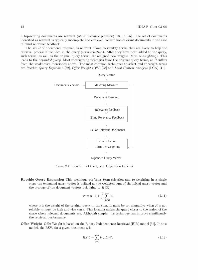
The queries formulated by the users are, on average, shorter than documents. This leads to more noisyterm distribution. The presence (absence) of a term does not necessarily mean that it is more (less)representative of the information need than others and this can result in significant over-estimation(under-estimation) of its weight in the query representation. This might cause a mismatch betweenthe term distribution in the relevant documents and in the query. Query expansion attempts to solvethis problem. It considers the query provided by the user as a tentative and changes it to make theretrieval operation more effective.

Statistics about terms occurring in relevant documents are required to expand the query. Toestimate such statistics, a set of relevant document is extracted with a preliminary retrieval processusing the initial query (as shown on figure 2.4). There are two ways to identify relevant documentsfrom the resulting ranking: either the user manually inspects the top-scoring documents and indentifysome of them as relevant (relevance feedback) [34], or the system automatically assumes that the


n top-scoring documents are relevant (blind relevance feedback) [13, 16, 25]. The set of documentsidentified as relevant is typically incomplete and can even contain non-relevant documents in the caseof blind relevance feedback.

The set R of documents retained as relevant allows to identify terms that are likely to help theretrieval process if included in the query (term selection). After they have been added to the query,such terms, as well as the original query terms, are assigned new weights (term re-weighting). Thisleads to the expanded query. Most re-weighting strategies favor the original query terms, as R suffersfrom the weaknesses mentioned above. The most common techniques to select and re-weight termsare Rocchio Query Expansion [32], Offer Weight (OW) [28] and Local Context Analysis (LCA) [41].

Documents Vectors

orRelevance feedback

Blind Relevance Feedback

Term Selection

Term Re−weighting

Query Vector

Expanded Query Vector

Matching Measure

Document Ranking

Set of Relevant Documents

Figure 2.4: Structure of the Query Expansion Process

Rocchio Query Expansion This technique performs term selection and re-weighting in a singlestep: the expanded query vector is defined as the weighted sum of the initial query vector andthe average of the document vectors belonging to R [32].

q′ = α · q +1R

∑

d∈R

d (2.11)

where α is the weight of the original query in the sum. It must be set manually: when R is notreliable, α must be high and vice versa. This formula makes the query closer to the region of thespace where relevant documents are. Although simple, this technique can improve significantlythe retrieval performance.

Offer Weight Offer Weight is based on the Binary Independence Retrieval (BIR) model [37]. In thismodel, the RSV, for a given document i, is:

RSVi =T∑

k=1

bi,k.OWk (2.12)


where, bi,k is 1 if term k is in document i and 0 otherwise and OWk is the Offer Weight ofterm k:

OWk = log

(P (k ∈ d|d ∈ R)P (k ∈ d|d ∈ R)

P (k /∈ d|d ∈ R)P (k /∈ d|d ∈ R)

)

where, P (k ∈ d|d ∈ R) (respectively P (k /∈ d|d ∈ R)) is the probability that term k is present(respectively not present) in a document, given that this document is relevant and P (k ∈ d|d ∈R) (respectively P (k /∈ d|d ∈ R)) is the probability that term k is present (respectively notpresent) in a document, given that this document is not relevant.The offer weight of a term k measures how helpful the presence of term k is to discriminaterelevant from non-relevant documents. The parameters of the OW are estimated as follows:

P (k ∈ d|d ∈ R) =rk

rand P (k ∈ d|d ∈ R) =

nk

n

where,r is the number of relevant documentsrk “ relevant documents containing term kn “ documents in the whole databasenk “ documents containing term k in the whole database

This leads to the following complementaries:

P (k /∈ d|d ∈ R) = 1− rk

rand P (k /∈ d|d ∈ R) = 1− nk

n

The OW hence corresponds to the following expression:

OWk = logrk(n− nk − r + rk)

(r − rk)(n− nk)

The offer weight is the criterion for term selection. Terms with higher OW are more likely tobe present in relevant documents than in non-relevant ones, they are hence added to the query.Re-weighting is also based on OW : the term-weights are multiplied by an increasing functionof their OW [28].

Local Context Analysis LCA has been introduced by Xu and Croft [41]. This technique selectsand re-weights terms based on their co-occurrences with the initial query terms. Renals et al.[26] proposed LCA in the following form:

LCA(e) = idfe

∑

t∈Q

idft

∑

i∈R

tft,i.tfe,i

where e is a potential expansion term, Q is the set of initial query terms and R is the set ofdocuments identified as relevant.Terms co-occuring with more query terms than others have an higher LCA value. Hence, co-occurence with all query terms is taken into account, which is more effective than consideringterm-by-term co-occurrence with single query terms separately. Term selection and term re-weighting then favor terms with higher LCA.

Rocchio Query Expansion was the first technique presented in the literature, followed by OW andLCA. These two are more flexible, as different strategies can be adopted to select and re-weight terms.Based on its probabilistic framework and its performance, OW is generally preferred.


2.2.5.3 Matching Measures and Ranking

In the Vector Space Model, the documents are ranked according to a matching measure. A matchingmeasure is a function that should associate good scores to couples of vectors representing documentswith similar content. As mentioned above, the only information extracted from documents is basedon their physical properties (e.g. term distribution) [18]. For this reason, all matching measurespresented in the literature take into account only the similarity of such properties. This is reasonableas two documents about the same topic are likely to use the same terms. However, it is also animportant limit because the same topic can be expressed with different terms.

In the ranking process, the matching measure between each document vector and the query isfirst computed. The documents are then ranked according to their matching with the query. Hence,documents better matching the query are considered more relevant.

Many matching measures can be interpreted as a scalar product:

RSVd =T∑

k=1

qk · dk (2.13)

where q = (q1, . . . , qT ) and d = (d1, . . . , dT ) are the query and document vector respectively.As mentioned in section 2.2.4, terms which best describe the document (or query) content should beassigned higher weights. Such terms would thus have an high influence on the scalar product. Thisallows the matching measure to be linked to content similarity. The most common weighting strategyis tf · idf (see equation 2.7).

Since queries are typically short, they lead to noisy tf estimates. To remove part of such noise,the queries can be binarized, i.e. only term presence or absence is taken into account. This often leadto better results [33]. The RSV formula is then:

RSVd =T∑

k=1

bq,k · tfd,k · idfk (2.14)

where tfd,k is the term frequency of term k in document d, idfk is the inverse document frequency ofterm k and bq,k is the binary weight of term k in the query.Since bq,k is 1 if term k is present in query and 0 otherwise, this formula can be rewritten:

RSVd =∑

k∈Q

tfd,k · idfk (2.15)

where Q is the set of query terms.In [29], two weaknesses of this formula are highlighted: first, the document length is not taken intoaccount and long documents are favored [36]. This is correct only if the longer a document is, moreit is relevant. But a document can also be long simply due to repetition. To deal with this problem,the formula can be modified as follows:

RSVd =∑

k∈Q

tfd,k · idfk

(1− b) + b ·NDL(d)(2.16)

where NDL(d) is the normalized document length of document d (length of document d dividedby the average length of a document) and b is an hyper-parameter (b ∈ [0, 1]). When b = 0, thedocument length is not considered. On the contrary, using b = 1 is equivalent to replacing the numberof occurrences of a term (tf) with the fraction of the length that the term represents in the document( tf

DL ).The second problem is that tf · idf weighting has a linear dependency on term frequency tf . A

term occurring twice in the document is not necessarily twice as much important as a term occuring


once. Better results can be obtained by smoothing the tf factor in case of multiple occurrences:

RSVd =∑

k∈Q

(K + 1).tfd,k.idfk

K + tfd,k(2.17)

where K is a hyper-parameter (K ∈ [0, +∞]).The combination of those two modifications leads to the so-called OKAPI formula [31]:

RSVd =∑

k∈Q

(K + 1) · tfd,k · idfk

K · ((1− b) + b ·NDL(d)) + tfd,k(2.18)

This formula is widely applied in state-of-the-art systems.

2.2.5.4 Recombination

Automatic segmentation of the database (see section 2.2.2) can lead to many short documents, whoseboundaries are not necessarily consistent with their content. For this reason, a relevant fraction ofthe text can be split across several documents. Such a fragmented part would be more valuable tothe user if presented as a single unit.

Recombination deals with such a problem: it takes as input the ranking of the documents, assegmented by the segmentation module, and gives as output a ranking of merged documents. Theprocess is performed in two steps. First, it should be decided which documents to merge. This decisionis based on the proximity in time and in the ranking. Inter-document similarity and difference betweenRSV can also be used. Second, the new documents resulting from merging should be assigned a RSVand ranked. The RSV can either be a function of the RSV of the original segments [16, 26] or can becomputed as the matching between the new document and the query. As well as providing a bettersegmentation to the user, recombination can also improve the retrieval process (e.g. a small segmentappearing near many relevant segments is likely to be relevant, even if its matching with the query islow).

2.3 Evaluation

Given a query, an IR system should ideally output a ranking in which all relevant documents appearbefore non-relevant ones. The performance of a system is measured by evaluating how close it is to thisideal condition. To perform such a task, there are different measures: each of them evaluates differentaspects of the system. Depending on the task the system is supposed to perform, some measures canbe more appropriate than others [3, chap. 3][27, chap.7]. However, the choice of a measure ratherthan another can be argued and performance evaluation is still an open problem [12].

The following subsections are organized as follows. Section 2.3.1 introduces Precision and Recall,the two fundamental measures in IR, Section 2.3.2 defines the Precision versus Recall curve andpresents different measures that can be extracted from it, Section 2.3.3 shows how measures definedfor a single query can be averaged to evaluate the system performance over a set of queries.

2.3.1 Precision and Recall

Precision P and Recall R are the two fundamental measures when dealing with the evaluation of anIR system, many other measures can be derived from them [3]. P and R are defined as follows:

P =|Hq ∩ Sq||Sq| (2.19)

R =|Hq ∩ Sq||Hq| (2.20)


where q is a given query, Sq is the set of documents identified as relevant by the system and Hq is theset of actually relevant documents (i.e documents judged as relevant by human assessors). P is thefraction of retrieved documents that are actually relevant and can be interpreted as the probabilitythat a retrieved document is actually relevant. R is the fraction of actually relevant documents thathave been identified as such by the system and can be interpreted as the probability of retrieving arelevant document.

Precision and Recall measure different aspects of the system, none of them gives an exhaustivedescription of the performance. To know recall (precision) does not give any information about preci-sion (recall). Different systems can have very different P (respectively R) at the same R (respectivelyP ) level. Both measures are hence necessary to evaluate a system, as a good system should achieveboth high precision and high recall.

In the context of a system relying on the vector space model, the output is not a set Sq ofdocuments identified as relevant by the system but a ranking. In this case, P and R are computed ateach position n in the ranking, considering that the n best ranked documents form the set Sq(n) ofretrieved documents:

P (n) =|Hq ∩ Sq(n)||Sq(n)| (2.21)

R(n) =|Hq ∩ Sq(n)|

|Hq| (2.22)

Along the ranking, the variations of P (n) and R(n) are not independent. When n increases, morerelevant documents are selected and R(n) increases. On the other hand, when n is higher, theprobability of including non-relevant documents in Sq(n) tends to be higher also, leading to a lowervalue of P (n).

2.3.2 Precision versus Recall Curve

As mentioned above, R(n) and P (n) are roughly inversely proportional. A good system should beable to achieve good precision levels, even at high recall levels. To evaluate this, the precision versusrecall curve is plotted.

Instead of plotting directly the P (n), R(n) couples for all n values, P is often first interpolated asa function of R.

P (r) = maxn:R(n)≥r

(P (n)) (2.23)

where r is an arbitrary recall level and P(r) is the interpolated precision value at such recall level. Theinterpolation allows to obtain P at any R level. Typically, precision is interpolated at 11 standardrecall values (r = 0, 10, 20, . . . , 100%).

Comparing plots is not as convenient as to compare single values. Different single value summariesare hence defined. Each of them gives a partial but meaningful information about the curve. Themost common measure is called average precision and is defined as follows:

avgP =1|Hq|

∑

n∈rel

P (n) (2.24)

where rel is the set of positions in the ranking corresponding to relevant documents.Another measure is the break-even point (BEP). Recall and precision are computed at position

|Hq| in the ranking, where |Hq| is the number of documents in the set Hq. At this position, P (n) andR(n) are equal and their value is called BEP. BEP can be seen as the intersection of the precisionversus recall curve and the axis bisector (R = P ).

A last measure is precision at position n, this measure is simply P (n) at a fixed n. This correspondsto the precision when the set Sq of selected documents is composed of the n top-ranked documents.This measure is important if, for example, the system displays to the user only the first n documentsof the ranking.


These three measures are not the only ones and many others can be defined [3, 27]. Each measurefocuses on different aspects of the performance. Some aspects can be more important than others,depending on the task the system is supposed to perform.

2.3.3 Averaging over Queries

All above presented measures have been defined to evaluate the system performance for a single query.But system evaluation involves a query set Q, which should be representative of all the queries thatcan be submitted to the system. The results obtained for each query must thus be averaged to evaluatethe system performance. There are two main techniques to perform such a task: micro-averaging andmacro-averaging.

In micro-evaluation, every individual document has the same influence on the measures obtained.Precision and recall are expressed as follows:

Pmicro =

∑q∈Q |Hq ∩ Sq|∑

q∈Q |Sq| (2.25)

Rmicro =

∑q∈Q |Hq ∩ Sq|∑

q∈Q |Hq| (2.26)

Then, Pmicro and Rmicro can be used to obtain precision versus recall curve as well as the single valuemeasures described before (section 2.3.2).

In macro-evaluation, every individual query has the same influence on the measures obtained. Thisis achieved by averaging over queries. Interpolated precision at a given recall level, average precisionand BEP are expressed as follows:

P (r) =1|Q|

∑

q∈Q

Pq(r) (2.27)

AvgPmacro =1|Q|

∑

q∈Q

AvgPq (2.28)

BEPmacro =1|Q|

∑

q∈Q

BEPq (2.29)

where Pq(r), AvgPq and BEPq are respectively interpolated precision at recall r, average precisionand break-even point computed for the individual query q.

Macro-evaluation is generally preferred in IR literature, whereas micro-evaluation is used in doc-ument categorization. In SDR, the macro-averages of BEP and AvgP are used in most works.However, these measures have been introduced in the context of text retrieval where the number ofdocuments in the database is constant. On the contrary in SDR, the number of documents variesdue to segmentation and recombination, this can influence the measure and this aspect has not beenextensively studied yet. Evaluation in IR, and even more in SDR, is not as well defined as in otherdomains and it remains an open problem.

2.4 Conclusion

In this chapter, the state-of-the-art in SDR has been presented. The structure of an SDR system hasbeen shown and the measures used for performance evaluation have been introduced.

The state-of-the-art approach to the SDR problem involves three main steps: recognition, segmen-tation and retrieval. At recognition step, a large vocabulary ASR system transcribes the speech datainto digital text. Transcribing into a stream of words rather than a stream of phonemes has beenshown more effective for the retrieval task. At segmentation step, the transcriptions are split intodocuments, which are the basic information units of retrieval. Segmentation typically uses a sliding


window to perform this task. At retrieval step, the documents that are relevant to a given query areretrieved. Retrieval is done using an IR system based on the VSM.

This approach to the SDR problem has shown to lead to good results with broadcast news data.However, the use of other kinds of data, such as corporate meetings, phone dialogs or academiclectures, might pose new problems: e.g. the recording conditions can lead the recognizer to introducemuch more noise, the lack of structure can make the segmentation process more difficult, etc..

The evaluation of SDR relies on standard IR measures. However, there is a significant differencebetween SDR systems and standard IR systems that can affect the evaluation process: an SDR systemsplits the database into documents during segmentation (and eventually modifies this split duringrecombination), while a standard IR system typically works with a manually segmented databaseand never modifies the provided segmentation. The variation in the number of documents affects allIR measures: the results obtained over two different segmentations of the same database are hencedifficult to compare. Having an IR measure independent from the segmentation would be of greatinterest.

Chapter 3

Experiments and Results

3.1 Introduction

The use of Information Retrieval (IR) systems over Automatic Speech Recognition (ASR) transcrip-tions has been proven effective to retrieve spoken data [11]. In this approach, the IR system considersthe spoken documents transcribed by the ASR system as a common digital text. However, a cor-pus of ASR transcriptions is very different from a corpus of clean texts on which IR systems usuallywork. The output of an ASR system is affected by recognition errors: some original words have beenreplaced by others (substitution errors), new words have been inserted (insertion errors) and someoriginal words have been lost (deletion errors). These errors are frequent (often, more than 25% ofthe words are recognized incorrectly) and an ASR transcription can hence be referred to as a noisytext. The effect of this noise on the retrieval process can be investigated by comparing the retrievalperformance over a noisy and a clean version of the same data.

In our work, this comparison is done using a broadcast news database (TDT2) [5] with a set ofretrieval queries (TREC SDR queries). The clean corpus is composed of manually produced transcrip-tions and the noisy corpus is composed of ASR transcriptions. Some standard IR measures (Precision,recall, break-even point, etc) have been used to evaluate the results of an SDR system on both corpora.

The following sections are organized as follows: section 3.2 presents the experimental setup and thedata used, section 3.3 shows the performances obtained with both clean and noisy data and comparethem and final section 3.4 draws some conclusions.

3.2 Experimental Setup

The SDR task is to find segments of a speech database that are relevant to an information needexpressed through a query. In our case, we consider a fully automatic approach, i.e. the user providesonly the query as opposed to interactive approaches (e.g. relevance feedback, see section 2.2.5.2).

In this context, an SDR system has two inputs: a database of speech recordings and a set ofqueries. We used Topic Detection and Tracking 2 (TDT2) [5] database and the queries collected forTREC SDR evaluation (i.e. benchmark queries used at the Spoken Document Retrieval session of theText Retrieval Conference in 1999 and 2000) [11].

The TDT2 database is composed of 600 hours of broadcast news, which is sufficiently large tohave a non-trivial retrieval task (i.e. for a given query, the relevant documents should represent onlya small percentage, less than 2% for TREC queries, of the whole collection). Moreover, in TDT2,both reference transcriptions and ASR transcriptions are available, which allows one to investigate theeffect of recognition errors on the retrieval performance. The query set contain 100 elements. Thesequeries were used at the TREC-9 conference with a predefined split into training and test set. Weused the same split to compare our results with those obtained over the same data.

19


The following subsections are organized as follows, section 3.2.1 presents TDT2 and section 3.2.2outlines the queries used.

3.2.1 TDT2 Database

The TDT2 database [5] is composed of 600 hours of broadcast news in American English. TDT2 hasbeen designed to include six months (from January 4 to June 30, 1998) of material drawn on a dailybasis from four sources (two TV channels, CNN and ABC, and two radio stations, PRI and VOA).Each day an audio segment of fixed length has been recorded from each source. The length variesbetween 30 and 60 minutes depending on the source.

For each audio segment, two different transcriptions are available: the first one has been manuallyproduced (closed-caption) and the other one is obtained with an Automatic Speech Recognition (ASR)system1. The closed-caption is considered as clean text, even if it is affected by a Word Error Rate(WER) of ∼10%. The ASR output has a ∼30% WER and plays the role of a noisy text.

Moreover, each of the recordings has been manually segmented into news stories that are usedas documents (i.e segment of speech containing homogeneous content, as defined in section 2.2.2).The manual segmentation allows one to perform the retrieval task without taking into account theautomatic segmentation problem.

There are approximately 21,500 documents in the manual segmentation provided with the database.Their length distribution (see figure 3.1) shows the distinction between two classes of documents: theshort ones (around 50 words) and the long ones (around 160 words). This is important when consid-ering the retrieval process because most matching measures are influenced by length variability (seesection 2.2.5.3).

3.2.2 TREC SDR Queries

In order to evaluate an IR system, it is necessary to have a set of queries with related relevancejudgments. During the TREC SDR evaluation, two sets of 50 queries have been collected for TDT2:a training set (also called TREC-8) and a test set (also called TREC-9). The use of such sets allowsone to compare the results obtained by other groups following the same protocol.

The distribution of the number of relevant documents per query (see figure 3.2) shows that thereare never more than 1.1% of the documents that are relevant to a given query. The task is hencedifficult because the probability of retrieving randomly a relevant document is less than 1.1%.

In general, queries are shorter than documents and this applies to TREC queries: the averagequery-length is 6.3 words while the average document-length is 178.7 words. This is important becausematching measures and query expansion techniques consider this characteristic (see sections 2.2.5.3and 2.2.5.2).

3.3 Experiments and Results

The presence of noise in the data is likely to affect the effectiveness of IR systems. In this work,we compare the performance of a system when dealing with clean and noisy data. The differenceof effectiveness is measured through precision, recall and other derived measures. The system weused is based on the Vector Space Model (VSM) and its structure is similar to the one described insection 2.2. Recognition and segmentation modules are simulated by the use of transcriptions andsegmentation provided with TDT2 while the other modules (normalization, indexing and retrieval)have been implemented.

The following sections are organized as follows, section 3.3.1 presents the results obtained withclean transcriptions and section 3.3.2 shows the results obtained with the noisy transcriptions andcompares them with the preceeding ones.

1A state-of-the-art ASR system of Dragon Systems trained on Hub4 database


Document Length Distribution

100 200 300 4000

50

100

150

200

250

300

350

Document length

Num

ber

of d

ocum

ents

Figure 3.1: Document Length Distribution. There are two classes of documents: the short ones(around 50 words) and the long ones (around 160 words).

Number of Relevant Documents per Query

0 50 100 150 200 250 3000

5

10

15

Number of relevant documents for a query

Num

ber

of q

uerie

s

Figure 3.2: Relevant Documents per Query Distribution. There are never more than 1.1% of thedocuments that are relevant to a given query.


3.3.1 Clean Text

The clean documents used in these experiments are closed-captions segmented with TDT2 manualsegmentation (as explained in section 3.2.1). We perform different measurements at different steps(normalization, matching measure and query expansion) of the process. This allows us to have areference to evaluate the effect of the noise on different modules of the system.

In a system based on the VSM, the documents are represented by vectors. Each componentof a vector is a function of the frequency of an index term in the documents (see section 2.2.4).Normalization performs the extraction of the index terms (see section 2.2.3). It is hence important tomeasure the number of index terms and their frequencies after normalization as they influence all thefollowing retrieval process.

The document/query matching measure corresponds to the RSV, the criterion to rank the doc-uments in order of relevance. The document with the highest (lowest) matching with the query areidentified as relevant (non-relevant) (see section 2.2.5.3). Using a matching measure rather than an-other can affect significantly the system performance. We used the OKAPI formula (equation 2.18),which is widely applied in the literature. OKAPI is an evolution of the tf · idf matching measure andwe evaluate the improvement of the performance it is supposed to give.

Query expansion is a step that aims at modifying the query to make it more effective. However,there is not a single technique to perform query expansion and the performances of each techniquedepends on the task. For this reason, we compared the performance obtained with different techniques.

The following sections are organized as follows, section 3.3.1.1 presents the effect of normalization,section 3.3.1.2 describes the effectiveness of the OKAPI formula compared to the standard tf · idfmatching measure and section 3.3.1.3 shows the results obtained with different query expansion tech-niques.

3.3.1.1 Normalization Effect

As explained in section 2.2.3, normalization removes any variability which is not helping the retrievalprocess. To perform this task, the stream of words (i.e. the ASR output or the closed caption text) ofeach document is stopped and stemmed. Stopping is performed using a generic stoplist of 389 words.Once these words have been removed, the remaining words are replaced with their stems using Porteralgorithm [24]. The documents are then available in their normalized form, i.e a stream of indexterms.

Compared to the document collection before normalization, the total number of words in thedatabase has been reduced by 51% after stopping (see table 3.1), while stemming results in a lexiconwith 34% less terms (see table 3.2).

Before Stopping After Stopping ReductionNumber of words 3,862,325 words 1,880,460 words 51%

Table 3.1: Corpus Reduction by Stopping

Before Stemming After Stemming ReductionNumber of terms 57,141 words 37,961 words 34%

Table 3.2: Lexicon Reduction by Stemming

The distribution of document frequencies df (i.e the number of documents in which a term appear)is also measured, as it is used in most matching measures to give more or less weight to a term. Infact, the terms with lower document frequency are given more weight in document representation,rare terms being considered as more discriminant. As shown on figure 3.3, rare terms represent an


important part of the lexicon: for example, 50% of the terms in the lexicon are present in 3 documentsor less. However, this distribution should be examined cautiously as it is affected by errors that occurduring manual transcription. These typing errors typically result in a term that differ from the exactone by one letter, which leads to many terms that occur once in the database (e.g. in one documentpresident has been transcribed into prdsident).

3.3.1.2 Matching Measure Effectiveness

The document/query matching measure is used to compute the RSV of a document. The RSV shouldideally be higher for relevant documents than for non-relevant ones. Different matching measures tryto achieve that goal with different effectiveness. We compared two of them: a simple tf · idf approach(equation 2.15) and the OKAPI formula (equation 2.18).

The OKAPI formula should lead to better results as it is an improvement of the tf · idf formulawhich takes document length into account and smoothes the tf factor. The results (table 3.3 andfigure 3.4) show that this is clearly verified: the system using the OKAPI matching measure performssignificantly better than the one using the simple tf · idf approach (Both AvgP and BEP are ∼75%higher). The OKAPI matching measure will hence be used for all the following experiments.

Baseline OKAPIAvgP 19.1% 35.6%BEP 20.6% 35.4%

Table 3.3: AvgP and BEP using baseline and OKAPI matching measure

3.3.1.3 Query Expansion Effectiveness

Query expansion (QE) is an optional step that attempts to make the query more effective. To performsuch a task, a set R of documents identified as relevant is first extracted from a preliminary ranking,then this set is used to identify terms that can be added to the original query. As we use blindrelevance feedback, R corresponds to the documents at the |R| first positions in the ranking. Threemain techniques are available to select the expansion terms and obtain the new query: Rocchio QE,LCA and OW (see section 2.2.5.2). Each of them has been tested.

The results (see table 3.4 and figure 3.5) show that all QE techniques increase the performancesignificantly compared to the system without QE. However, no technique is significantly better thanthe others: Rocchio QE, LCA and OW lead to similar performance.

no QE Rocchio LCA OWAvgP 35.6% 42.1% 42.6% 41.1%BEP 35.4% 41.3% 40.5% 39.0%

Table 3.4: AvgP and BEP for different Self QE techniques on clean text

In blind relevance feedback, the size of the set R used to identify expansion terms is typicallysmall because the only documents that can be reliably identified as relevant are those appearing atthe very top positions of the ranking. This can be a problem: when R is too small, this can result inthe selection of terms that are fitted to the documents present in the set.

Parallel QE attempts to solve this problem. In this case, the preliminary ranking is obtained usinganother corpus (the parallel corpus, which is independent from the self corpus, i.e. the corpus onwhich the system works). If the parallel corpus contains more relevant documents, the system is likelyto output a ranking in which the same precision level is achieved at lower positions in the ranking.This allows the extraction of a bigger set R.


Document Frequency Distribution

20 40 60 80 1000

2000

4000

6000

8000

Document frequency

Num

ber

of te

rms

Figure 3.3: Document Frequency Distribution for clean text (Truncated at df=100). Rare termsrepresent an important part of the lexicon: 50% of the terms in the lexicon are present in 3 documentsor less.

Precision vs Recall

0 20 40 60 80 1000

10

20

30

40

50

60

70

80

Recall (%)

Pre

cisi

on (

%)

OKAPIBaseline

Figure 3.4: Precision vs Recall using baseline and OKAPI matching measure on clean text. The systemusing the OKAPI matching measure performs significantly better than the one using the simple tf ·idfapproach.


Precision vs Recall

0 20 40 60 80 1000

10

20

30

40

50

60

70

80

Recall (%)

Pre

cisi

on (

%)

no QERocchioLCAOW

Figure 3.5: Precision vs Recall for different Self QE techniques on clean text. All QE techniques havesimilar performances and they lead to significantly better results than the system without QE

In our case, we use a parallel corpus of newswire (TDT2 newswire) covering the same period as ourspoken database (TDT2). As the same kind of topics are present in the two corpora, we suppose thedensity of relevant documents to be the same (∼1% depending on the query). As the parallel corpusis bigger than TDT2 (∼14 million words compared to ∼4 million words), it should hence contain morerelevant content.

Parallel QE (table 3.5 and figure 3.6) has a lower performance than self QE (table 3.4 and figure3.5). The assumption that TDT2 newswire contains more relevant content might then be wrong.Another possibility can be that the system does not identify relevant documents in the parallel corpusas well as it does in the self corpus. This is certainly the case as the OKAPI formula parameterscannot be tuned for the parallel corpus (no relevant judgment are available for this corpus). However,Parallel QE is still improving the performance compared to a system without QE.


Table 3.5: AvgP and BEP for different Parallel QE techniques on clean text

This means that the parallel-expanded query (i.e. the query expanded with the parallel corpus) ismore effective than the original one. Hence, self QE performance should be improved if parallel QE isperformed before, i.e. if the input of self QE is the parallel-expanded query rather than the originalquery. The results obtained (table 3.6) show that parallel QE followed by self QE is performing betterthan self QE alone.


Precision vs Recall

0 20 40 60 80 1000

10

20

30

40

50

60

70

80

Recall (%)

Pre

cisi

on (

%)

no QERocchioLCAOW

Figure 3.6: Precision vs Recall for different Parallel QE techniques on clean text. Parralell QE improvethe performance compared to a system without QE.

no QE self QE parallel + self QEAvgP 35.6% 42.6% 45.2%BEP 35.4% 40.5% 42.9%

Table 3.6: AvgP and BEP when using parallel QE before self QE on clean text (LCA is used for bothParallel and Self QE)


3.3.2 Noisy Text

The noisy text corresponds to ASR transcriptions (∼30% WER) as provided with TDT2. They havebeen segmented into documents using the database manual segmentation (see section 3.2.1). Thesame experiments have been done using the noisy documents to compare with the results obtained onclean text.

The following sections are organized as follows, section 3.3.2.1 presents the effect of normalization,section 3.3.2.2 describes the effectiveness of the OKAPI formula compared to the standard tf · idfmatching measure and section 3.3.2.3 shows the results obtained with different query expansion tech-niques.

3.3.2.1 Normalization Effect

Normalization is performed the same way as with clean text. Its effect is the same: stopping reducesthe total number of words by 50% (table 3.7), while stemming results in a lexicon with 38% less terms(table 3.8). However, the total number of words is not the same due to insertion and substitutionerrors introduced by the recognizer. The lexicon size is also modified due to the limited vocabury ofthe recognizer. The noisy documents can only contain words that are present in the ASR vocabulary(∼38,000 different words), in consequence, index terms can only be stems of these words.

Before Stopping After Stopping ReductionNumber of words 3,841,053 words 1,859,893 words 50%

Table 3.7: Corpus Reduction by Stopping

Before Stemming After Stemming ReductionNumber of terms 37,696 words 23,099 words 38%

Table 3.8: Lexicon Reduction by Stemming

The document frequency distribution (figure 3.7) obtained with noisy documents is similar to theone obtained with the clean ones except in the case of df = 1. The fact that the number of termsoccuring in one document is much bigger in the case of clean text is certainly due to errors in thehuman transcriptions rather than out of vocabulary problem in the ASR system. As mentioned insection 3.3.1.1, the errors present in the closed-caption transcription are typically typing errors whichresult in words appearing once in the database.

3.3.2.2 Matching Measure Effectiveness

The performances of the retrieval process when using a simple tf · idf matching measure and theOKAPI formula have been compared. OKAPI formula takes the document length into account andsmoothes the tf factor. As for clean documents, the length varies across documents (see section 3.2.1)and the tf factor is also overestimated in case of repetitions. OKAPI formula should also improve thesystem performance compared to the simple tf · idf formula in the case of noisy documents.

Results (table 3.9 and figure 3.8) show this improvement. Moreover, the effect of noise on theretrieval process can be measured: using the OKAPI formula average precision is 12% lower for noisydocuments than for clean ones (31.2% vs 35.6%), while BEP is 7% less (33.1% vs 35.4%).

3.3.2.3 Query Expansion Performance

Query expansion has shown to be effective in the case of clean text. For noisy text, the same experi-ments are presented, i.e. self QE and parallel QE have been tested alone and parallel QE followed by


Document Frequency Distribution

20 40 60 80 1000

1000

2000

3000

4000

Document frequency

Num

ber

of te

rms

Figure 3.7: Document Frequency Distribution for noisy text(Truncated at df=100). Most terms occuronly in few documents.

Precision vs Recall

0 20 40 60 80 1000

10

20

30

40

50

60

70

80

Recall (%)

Pre

cisi

on (

%)

OKAPIBaseline

Figure 3.8: Precision vs Recall using baseline and OKAPI matching measure on noisy text. As forclean text, the performance is significantly better when using the OKAPI formula.


Baseline OKAPIAvgP 17.8% 31.2%BEP 20.4% 33.1%

Table 3.9: AvgP and BEP using baseline and OKAPI matching measure

self QE is also evaluated.In the case of self QE, the set R of documents identified as relevant is extracted from the spoken

database. This means that this set R is also affected by recognition errors. However, the selection ofexpansion terms from the set should be robust to the noise as the set R contains different documentsthat should not contain the same errors. The results obtained (table 3.10 and figure 3.9)


Table 3.10: AvgP and BEP for different Self QE techniques on noisy text

The parallel expanded query is more effective than the self expanded query if a better preliminaryranking is obtained with the parallel corpus. As for clean text, this better ranking is not obtained andparallel QE does not lead to performance as good as self QE (table 3.11 and figure 3.10). However,parallel QE improves the process when compared with the system without QE.


Table 3.11: AvgP and BEP for different parallel QE techniques on noisy text

As the parallel expanded query performs better than the original one, this query is used to makethe preliminary ranking of self QE. The measures show that the improvement obtained with thisapproach is not significant contrary to the results on clean documents.

no QE self QE parallel + self QEAvgP 31.2% 40.2% 41.2%BEP 33.1% 39.5% 40.1%

Table 3.12: AvgP and BEP when using parallel QE before self QE on clean text (LCA is used forboth Parallel and Self QE)

As for clean documents, the performance improvement obtained with QE is important (AvgP is32% higher, 41.2% vs 31.2%, and BEP is 20% higher, 40.1% vs 33.1%, when parallel QE followed byself QE is compared to the results without query expansion).

The effect of noise on the final system, including OKAPI formula, QE expansion on parallel corpusfollowed by query expansion on the self corpus is still significant (see table 3.13). However, the qualityof clean transcritpion (10% WER) and noisy transcription (30% WER) are very different and even anoisy transcritpion affected by recognition errors allows one to achieve satisfying results.


Precision vs Recall

0 20 40 60 80 1000

10

20

30

40

50

60

70

80

Recall (%)

Pre

cisi

on (

%)

no QERocchioLCAOW

Figure 3.9: Precision vs Recall for different Self QE techniques on noisy text. QE improve significantlythe performance. All QE techniques lead to similar results.

Precision vs Recall

0 20 40 60 80 1000

10

20

30

40

50

60

70

80

Recall (%)

Pre

cisi

on (

%)

no QERocchioLCAOW

Figure 3.10: Precision vs Recall for different parallel QE techniques on noisy text. The parallelexpanded query perform, on average, better than the original one.


Clean Noisy Relative DifferenceAvgP 45.2% 41.2% 9%BEP 42.9% 40.1% 7%

Table 3.13: Comparison of noisy and clean results when using parallel QE and self QE

3.4 Conclusion

The use of an IR system over noisy texts has been experimented in this work. An SDR system basedon the VSM has been used to compare the performance obtained over clean and noisy transcriptionsof a speech database. The database used is TDT2 (600 hours broadcast news), the clean version of thecorpus is composed of manual transcriptions (closed-captions), while the noisy version is the outputof an ASR system. The effect of noise has been measured at the main steps of the retrieval process(normalization, matching measure and query expansion).

Normalization has a similar effect on clean and noisy data (The reduction of the total number ofwords by stopping is ∼50% and the reduction of the lexicon size by stemming is ∼35%). The onlyobserved difference is that the limited vocabulary of the ASR system leads to a smaller lexicon.

At the retrieval step, the performances obtained with the OKAPI matching measure are lowerwith noisy data (31.2% vs 35.6% in average precision), but the OKAPI formula is leading to betterresults than tf · idf over both clean and noisy texts (∼75% improvement in average precision in bothcases). The different query expansion techniques have led to significant improvement with both cleanand noisy data. Parallel QE has been shown less useful with the noisy documents.

The best performance achieved on noisy data is obtained when using OKAPI formula and bothself and parallel QE (41.2% average precision). The results obtained in this work are comparablewith those published at the TREC-9 conference (where average precision values vary from 43.2% and46.2% over the same noisy data [13, 16, 25]). The better results obtained by the other groups areprobably due to the corpus used for query expansion which is significantly bigger than ours for all ofthem

As mentioned in section 3.2.1, 3 words out of 10 are mis-recognized in the noisy corpus (i.e 30%WER) while less than 1 word out of 10 is mis-transcribed in the clean corpus. Compare to thissignificant difference of quality in the transcription, the difference of performance is quite limited(average precision is 9% lower for noisy data when using OKAPI formula and both self and parallelQE). Some recognition errors might have only a limited impact, while others should be more important.This point should be investigated in the future.


Chapter 4

Conclusions and Future Work

The topic of this thesis is Spoken Document Retrieval (SDR). State-of-the-art SDR systems use ASRto transcribe speech data into digital text and then perform retrieval on it. The ASR process is notperfect and introduces a significant amount of noise (i.e. words that are incorrectly recognized). AnSDR system has been implemented to investigate the effect of this noise on the main step of theretrieval process.

It has been shown at normalization step that stopping has the same effect on clean and noisy data(corpus reduction is ∼50% in both cases). This means that recognition errors occur as frequently onstop-words as on content words. Also, the effect of stemming is similar (lexicon reduction is ∼35%in both cases) which means that the vocabulary of the clean text and the vocabulary of the noisytranscription have a similar distribution of inflected forms per stem. The only significant differenceobserved is in the dictionary size: the lexicon is smaller in the noisy text due to the limited vocabularyof the ASR system and to the presence of errors in the closed-caption transcription resulting in manyspurious words appearing once in the database.

The matching measure we used is the OKAPI formula. It has been shown that with both clean andnoisy data the OKAPI formula performs significantly better than the wide-spread tf · idf . Comparedto tf ·idf , OKAPI takes into account the document length and reduces the influence of term repetition.This relies on the hypotheses that longer documents are not richer in content and that a repetition isnot as important as the first occurrence of a term. These hypotheses are verified in both cases.

The last step of the retrieval process we investigated is Query Expansion (QE). Two kinds ofexpanded query have been considered: self-expanded and parallel-expanded. Compared to the ap-proach without QE, both techniques lead to a significant improvement over clean and noisy text. Theselection of good expansion terms is possible even from noisy documents, as shown in the case of selfQE over noisy data. This happens, in our opinion, because the redundancy across the documentsused for QE improves the robustness with respect to recognition errors. The parallel-expanded queryhas been shown less effective for noisy data than for clean one. The parallel QE results are howeverdata-dependent and other results might have been obtained with a different parallel database.

In all the experiments, clean data leads to better results. However, the transcription errors intro-duced by the ASR system degrade only slightly the retrieval effectiveness (e.g. ∼7% degradation forbreak-even point), even if the clean and noisy corpora are very different (10% vs 30% WER). Thenoise seems to have a limited impact on the performance. At the error rate of our data, an IR systemdeveloped for clean text is effective over noisy data.

Several interesting issues remain open and can be subject of future work. The information con-tained in speech is not limited to a text transcription. Dialog dynamics, speaker turns, etc areneglected by the approach based on the simple transcription. Introducing such information could helpthe retrieval process. Furthermore, most research has been done on broadcast news, which is only aspecific kind of data. Broadcast news data have good recording conditions, a topic-based structure,read speech without hesitation, emotion, etc. These characteristics help both the recognition and

33


the retrieval steps. Using other types of data such as academic lectures, phone dialogs or corporatemeetings can pose interesting problems.

Bibliography

[1] Akiko Aizawa. An Information-Theoretic Perspective of Tf-Idf Measures. Information Processingand Management, Vol.39, No.1, 45–65, 2003.

[2] J. Ajmera, I. McCowan, and H. Bourlard. Robust HMM-based Speech/Music Segmentation.Proceedings of ICASSP, 2002.

[3] Ricardo A. Baeza-Yates and Berthier A. Ribeiro-Neto. Modern Information Retrieval. ACMPress / Addison-Wesley, 1999.

[4] D. Beeferman, A. Berger, and J. Lafferty. Statistical Models for Text Segmentation. MachineLearning Journal Special Issue on Natural Language, 1999.

[5] C. Cieri, D. Graff, M. Liberman, N. Martey, and S. Strassel. The TDT-2 Text and Speech Corpus.Proceedings of DARPA Broadcast News Workshop, 1999.

[6] F. Crestani, M. Lalmas, C.J. Van Rijsbergen, and Campbell I. Is This Document Rele-vant?. . . Probably: A Survey of Probabilistic Models in Information Retrieval. ACM ComputingSurveys, 30(4), 1998.

[7] S. Dumais. Enhancing Performance in Latent Semantic Indexing Retrieval. Behavior ResearchMethods, Instruments and Computers, 1991.

[8] C. Fox. Lexical Analyis and Stoplist. In Information Retrieval: Data Structures and Algorithms.Prentice Hall, 1992.

[9] W.B. Frakes. Stemming Algorithms. In Information Retrieval: Data Structures and Algorithms.Prentice Hall, 1992.

[10] N. Fuhr. Probabilistic Models in Information Retrieval. The Computer Journal, 35 (3): 243-255,1992.

[11] J. S. Garofolo, C. G. Auzanne, and E. Voorhees. The TREC Spoken Document Retrieval Track:A Success Story. Proceedings of Content-Based Multimedia Information Access Conference, 2000.

[12] J. S. Garofolo, E. M. Voorhees, C. G. Auzanne, and V. M. Stanford. Spoken Document Retrieval:1998 Evaluation and Investigation of New Metrics. Proceedings of the ESCA ETRW workshop,1998.

[13] J. L. Gauvain and G. Adda Y. de Kercardio L. Lamel, C. Barras. The LIMSI SDR system forTREC-9. Proceeding of TREC-9, 2000.

[14] D. Hand, H. Mannila, and P. Smyth. Data Mining. MIT Press, 2001.

[15] F. Jelinek. Statistical Aspects of Speech Recognition. MIT Press, 1997.

[16] S.E. Johnson, P. Jourlin, K. Sprck Jones, and P.C. Woodland. Spoken Document Retrieval forTREC-9 at Cambridge University. Proceeding of TREC-9, 2000.

35


[17] Guillaume Lathoud, Iain A. McCowan, and Darren C. Moore. Segmenting Multiple ConcurrentSpeakers Using Microphone Arrays. Proceedings of Eurospeech 2003, 2003.

[18] H.P. Luhn. The Automatic Creation of Litterature Abstracts. IBM Journal of Research andDeveloppement, 2(2):159–165.

[19] H.P. Luhn. The Automatic Derivation of Information Retrieval Encodements from Machine-Readable Texts. Information Retrieval and Machine Translation, 3(2):1021–1028, 1961.

[20] C.D. Manning and H. Schutze. Foundations of Statistical Natural Language Processing. MITPress, 1999.

[21] I. McCowan, S. Bengio, D. Gatica-Perez, G. Lathoud, F. Monay, D. Moore, P. Wellner, andH. Bourlard. Modeling Human Interaction in Meetings. Proceedings of International Conferenceon Acoustics, Speech and Signal Processing, 2003.

[22] C. Ng, R. Wilkinson, and J. Zobel. Experiments in Spoken Document Retrieval using PhonemeN-grams. Speech Comunication, 32:61–77, 2000.

[23] K. Ng. Towards Robust Methods for Spoken Document Retrieval. Proceedings of ICSLP 1998,1998.

[24] M. F. Porter. An Algorithm for Suffix Stripping. Program, 14(3):130–137, 1980.

[25] S. Renals and D. Abberley. The THISL SDR system at TREC-9. Proceedings of TREC-9, 2001.

[26] S. Renals, D. Abberley, D. Kirby, and T. Robinson. Indexing and Retrieval of Broacast News.Speech Communication, 32:5–20, 2000.

[27] C. J. Van Rijsbergen. Information Retrieval, 2nd edition. Butterworths, 1979.

[28] S. Robertson. On Term Selection for Query Expansion. Journal of Documentation, 46:359–364,1990.

[29] S. Robertson and K. Sparck Jones. Simple Proven Approaches to Text Retrieval. Tech. Rep.TR356, Cambridge University Computer Laboratory, 1997.

[30] S. Robertson, S. Walker, and M. Beaulieu. Experimentation as a way of life: Okapi at TREC.Information Processing and Management, 2000.

[31] S. Robertson, S. Walker, M. Hancock-Beaulieu, A. Gull, and M. Lau. Okapi at TREC 3. Pro-ceedings of Text REtrieval Conference, 1992.

[32] J.J. Rocchio. Relevance Feedback in Information Retrieval. In The SMART Retrieval System:Experiments in Automatic Document Pocessing, pages 313–323. Prentice Hall.

[33] G. Salton and C. Buckley. Term Weighting Approaches in Automatic Text Retrieval. InformationProcessing and Management, 24(5):513, 1988.

[34] G. Salton and C. Buckley. Improving Retrieval Performance by Relevance Feedback. Journal ofthe American Society of Information Science, 41:288–297, 1990.

[35] G. Salton, A. Wong, and C.S. Yang. A Vector Space Model for Automatic Indexing. Communi-cations of the ACM, 18, 1975.

[36] A. Singhal, G. Salton, M. Mitra, and C. Buckley. Document Length Normalization. InformationProcessing and Management, 32(5):619–633, 1996.


[37] K. Sparck-Jones, S. Walker, and S. Robertson. A Probabilistic Model of Information Retrieval:Development and Status. Cambridge University Technical Report TR-446, 1998.

[38] P. Srinivasan. Thesaurus construction. In Information Retrieval: Data Structures and Algorithms.Prentice Hall, 1992.

[39] S. Wartik. Boolean Operations. In Information Retrieval: Data Structures and Algorithms.Prentice Hall, 1992.

[40] Ian H. Witten, Alistair Moffat, and Timothy C. Bell. Managing Gigabytes: Compressing andIndexing Documents and Images. Morgan Kaufmann Publishers, 1999.

[41] J. Xu and W. B. Croft. Querying expansion using local and global document analysis. Proceedingsof the 19th International Conference on Research and Development in Information Retrieval,1996.


Acknowledgments

The authors wish to thank the Swiss National Science Foundation for supporting this work throughthe National Center of Competence in Research (NCCR) on Interactive Multimodal InformationManagement (IM2).

39

Date post:	11-Feb-2022
Category:	Documents
Upload:	others
View:	1 times
Download:	0 times