AUT Journal of Modeling and Simulation AUT J. Model. Simul., 49(1)(2017)13-22 DOI: 10.22060/miscj.2016.838 An Application of Genetic Network Programming for Pricing of Basket Default Swaps (BDS) A. Esfahanipour * and R. Jahanbin Department of Industrial Engineering & Management Systems, Amirkabir University of Technology, Tehran, Iran ABSTRACT: The credit derivative market has experienced a remarkable growth over the past decade. As such, there is a growing interest in tools for pricing of the most prominent credit derivative, the credit default swap (CDS). In this paper, we propose a heuristic algorithm for pricing of basket default swaps (BDS). For this purpose, genetic network programming (GNP), which is one of the most recent evolutionary methods with graph structure as a subgroup of machine learning methods, is applied to assess basket default swap spreads. Here GNP is an alternative way to model the default correlation structure among different reference entities in a basket default swap. In order to improve the efficiency of the proposed algorithm, GNP with the vigorous connection (GNP-VC) is developed and used for the first time in this paper. To implement our model, we consider a basket consisting of 25 entities of the CDX. NA.IG.5Y index. We compare the heuristic results with the Monte Carlo ones and discuss the efficiency of the proposed algorithm.The impact of vigorous connection on the performance of GNP is also reported. Review History: Received: 1 February 2016 Revised: 10 April 2016 Accepted: 12 November 2016 Available Online: 18 November 2016 Keywords: credit default swap (CDS) basket default swaps (BDS) default correlation genetic network programming(GNP) genetic network programing with vigorous connection (GNP-VC) 13 1- Introduction Credit derivatives have become increasingly important financial instruments during the last decade. Their market has grown significantly since their inception in the mid-1990s. Credit derivatives are flexible and efficient instruments which allow users to isolate credit risk from other quantitative and qualitative factors associated with owning an exposure. Hence, they can be used to transfer and hedge credit risk in an efficient and flexible manner, customized to a client’s requirements. Credit risk includes not just default or insolvency risk but also changes in credit spreads and thereby market values, changes in credit ratings and generic changes in credit quality. Credit derivatives are swaps, forward and option contracts, particularly credit default swaps (CDS); which can be used to hedge against all these types of credit risks, see Bomfim [3]. Credit default swaps (CDS) have been proven to be one of the most successful financial innovations of the 1990s. It is an instrument that provides insurance against the default of a particular company (or sovereign entity) on its debt. The company is known as the reference entity, and the default is known as a credit event. The buyer of protection pays periodic payments to the seller of protection at a predetermined fixed rate per year. The payments continue until the maturity of the contract or until the occurrence of a credit event, whichever is earlier. If a default event occurs, the buyer of protection has the right to deliver to the seller of protection a bond issued by the reference entity in exchange for its face value. Figure 1 shows a simple example of CDS. A common question when considering the use of credit derivatives, as an investment or a risk management tool, is how they should be priced. In general, the pricing of a credit default swap will depend on the credit quality of the reference entity and the length of the swap contract. When it comes to pricing of basket default swaps, modeling of the dependence structure of credit risks is a crucial problem. This problem arises from the effect of one entity default on other correlated entities. Therefore, the default correlations must be considered in the process of pricing which increases the complexity of the problem. There are different methods in the modeling of default correlation in the literature which could be categorized into three approaches: copula, conditional independence, and contagion. Most of these models use simplifying assumptions which decrease the comprehensiveness of the approach, see Takada, Sumita [36] and SchröTer, Heider [34]. As a case in point, copula assumes a specific distribution function for default times of individual assets, or the Markov process in contagion models considers a particular distribution function for states which could not be dominated for all assets, see Choe, Jang [4] and Wu [38]. In this paper, we propose a machine learning algorithm for the basket default swaps pricing which uses financial parameters as inputs and does not apply statistical simplifying assumptions, such as specific distribution function for default times. Machine learning algorithms are data-driven approaches to problem solving which can learn from and make predictions on data. Such algorithms operate by building a model from example inputs in order to make data-driven predictions or decisions rather than following strictly static program instructions. In the case of credit portfolio modeling, machine learning helps to find and learn default correlation structure through the learning phase. For this purpose, we use a recent graph structured heuristic method, named genetic network programming (GNP). In order to improve the efficiency of the proposed algorithm, GNP with a vigorous connection Corresponding author, E-mail: [email protected]
Transcript
AUT Journal of Modeling and Simulation
AUT J. Model. Simul., 49(1)(2017)13-22DOI: 10.22060/miscj.2016.838
An Application of Genetic Network Programming for Pricing of Basket Default Swaps (BDS)
A. Esfahanipour* and R. Jahanbin
Department of Industrial Engineering & Management Systems, Amirkabir University of Technology, Tehran, Iran
ABSTRACT: The credit derivative market has experienced a remarkable growth over the past decade. As such, there is a growing interest in tools for pricing of the most prominent credit derivative, the credit default swap (CDS). In this paper, we propose a heuristic algorithm for pricing of basket default swaps (BDS). For this purpose, genetic network programming (GNP), which is one of the most recent evolutionary methods with graph structure as a subgroup of machine learning methods, is applied to assess basket default swap spreads. Here GNP is an alternative way to model the default correlation structure among different reference entities in a basket default swap. In order to improve the efficiency of the proposed algorithm, GNP with the vigorous connection (GNP-VC) is developed and used for the first time in this paper. To implement our model, we consider a basket consisting of 25 entities of the CDX.NA.IG.5Y index. We compare the heuristic results with the Monte Carlo ones and discuss the efficiency of the proposed algorithm.The impact of vigorous connection on the performance of GNP is also reported.
Review History:
Received: 1 February 2016Revised: 10 April 2016Accepted: 12 November 2016Available Online: 18 November 2016
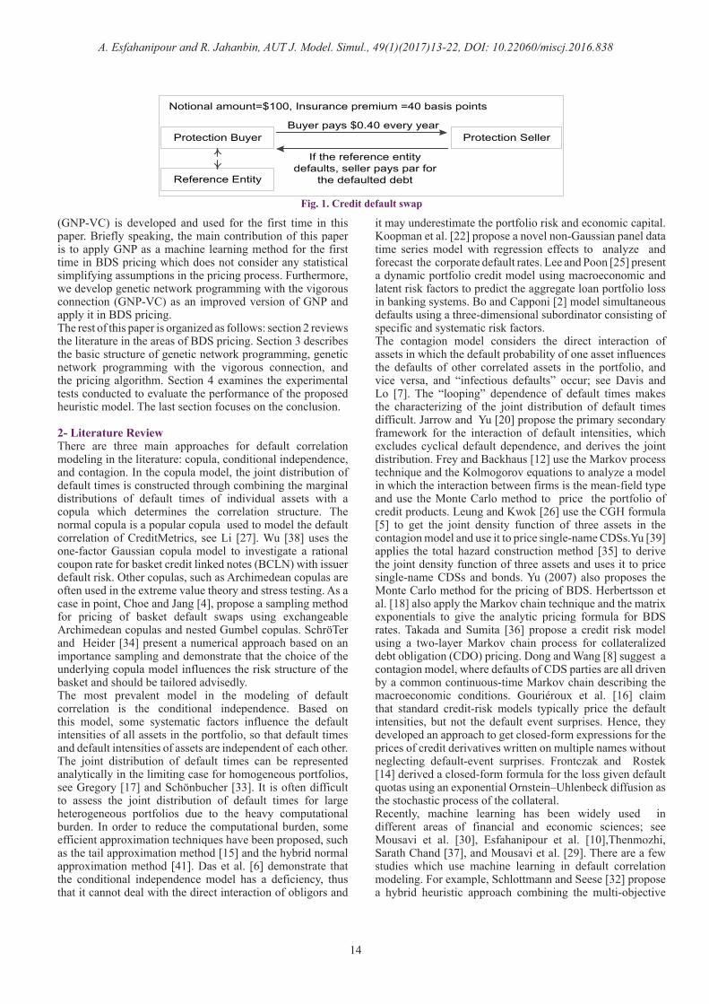
1- IntroductionCredit derivatives have become increasingly important financial instruments during the last decade. Their market has grown significantly since their inception in the mid-1990s. Credit derivatives are flexible and efficient instruments which allow users to isolate credit risk from other quantitative and qualitative factors associated with owning an exposure. Hence, they can be used to transfer and hedge credit risk in an efficient and flexible manner, customized to a client’s requirements. Credit risk includes not just default or insolvency risk but also changes in credit spreads and thereby market values, changes in credit ratings and generic changes in credit quality. Credit derivatives are swaps, forward and option contracts, particularly credit default swaps (CDS); which can be used to hedge against all these types of credit risks, see Bomfim [3]. Credit default swaps (CDS) have been proven to be one of the most successful financial innovations of the 1990s. It is an instrument that provides insurance against the default of a particular company (or sovereign entity) on its debt. The company is known as the reference entity, and the default is known as a credit event. The buyer of protection pays periodic payments to the seller of protection at a predetermined fixed rate per year. The payments continue until the maturity of the contract or until the occurrence of a credit event, whichever is earlier. If a default event occurs, the buyer of protection has the right to deliver to the seller of protection a bond issued by the reference entity in exchange for its face value. Figure 1 shows a simple example of CDS.A common question when considering the use of credit derivatives, as an investment or a risk management tool, is
how they should be priced. In general, the pricing of a credit default swap will depend on the credit quality of the reference entity and the length of the swap contract. When it comes to pricing of basket default swaps, modeling of the dependence structure of credit risks is a crucial problem. This problem arises from the effect of one entity default on other correlated entities. Therefore, the default correlations must be considered in the process of pricing which increases the complexity of the problem. There are different methods in the modeling of default correlation in the literature which could be categorized into three approaches: copula, conditional independence, and contagion. Most of these models use simplifying assumptions which decrease the comprehensiveness of the approach, see Takada, Sumita [36] and SchröTer, Heider [34]. As a case in point, copula assumes a specific distribution function for default times of individual assets, or the Markov process in contagion models considers a particular distribution function for states which could not be dominated for all assets, see Choe, Jang [4] and Wu [38].In this paper, we propose a machine learning algorithm for the basket default swaps pricing which uses financial parameters as inputs and does not apply statistical simplifying assumptions, such as specific distribution function for default times. Machine learning algorithms are data-driven approaches to problem solving which can learn from and make predictions on data. Such algorithms operate by building a model from example inputs in order to make data-driven predictions or decisions rather than following strictly static program instructions. In the case of credit portfolio modeling, machine learning helps to find and learn default correlation structure through the learning phase. For this purpose, we use a recent graph structured heuristic method, named genetic network programming (GNP). In order to improve the efficiency of the proposed algorithm, GNP with a vigorous connection
A. Esfahanipour and R. Jahanbin, AUT J. Model. Simul., 49(1)(2017)13-22, DOI: 10.22060/miscj.2016.838
14
(GNP-VC) is developed and used for the first time in this paper. Briefly speaking, the main contribution of this paper is to apply GNP as a machine learning method for the first time in BDS pricing which does not consider any statistical simplifying assumptions in the pricing process. Furthermore, we develop genetic network programming with the vigorous connection (GNP-VC) as an improved version of GNP and apply it in BDS pricing.The rest of this paper is organized as follows: section 2 reviews the literature in the areas of BDS pricing. Section 3 describes the basic structure of genetic network programming, genetic network programming with the vigorous connection, and the pricing algorithm. Section 4 examines the experimental tests conducted to evaluate the performance of the proposed heuristic model. The last section focuses on the conclusion.
2- Literature ReviewThere are three main approaches for default correlation modeling in the literature: copula, conditional independence, and contagion. In the copula model, the joint distribution of default times is constructed through combining the marginal distributions of default times of individual assets with a copula which determines the correlation structure. The normal copula is a popular copula used to model the default correlation of CreditMetrics, see Li [27]. Wu [38] uses the one-factor Gaussian copula model to investigate a rational coupon rate for basket credit linked notes (BCLN) with issuer default risk. Other copulas, such as Archimedean copulas are often used in the extreme value theory and stress testing. As a case in point, Choe and Jang [4], propose a sampling method for pricing of basket default swaps using exchangeable Archimedean copulas and nested Gumbel copulas. SchröTer and Heider [34] present a numerical approach based on an importance sampling and demonstrate that the choice of the underlying copula model influences the risk structure of the basket and should be tailored advisedly.The most prevalent model in the modeling of default correlation is the conditional independence. Based on this model, some systematic factors influence the default intensities of all assets in the portfolio, so that default times and default intensities of assets are independent of each other. The joint distribution of default times can be represented analytically in the limiting case for homogeneous portfolios, see Gregory [17] and Schönbucher [33]. It is often difficult to assess the joint distribution of default times for large heterogeneous portfolios due to the heavy computational burden. In order to reduce the computational burden, some efficient approximation techniques have been proposed, such as the tail approximation method [15] and the hybrid normal approximation method [41]. Das et al. [6] demonstrate that the conditional independence model has a deficiency, thus that it cannot deal with the direct interaction of obligors and
it may underestimate the portfolio risk and economic capital. Koopman et al. [22] propose a novel non-Gaussian panel data time series model with regression effects to analyze and forecast the corporate default rates. Lee and Poon [25] present a dynamic portfolio credit model using macroeconomic and latent risk factors to predict the aggregate loan portfolio loss in banking systems. Bo and Capponi [2] model simultaneous defaults using a three-dimensional subordinator consisting of specific and systematic risk factors.The contagion model considers the direct interaction of assets in which the default probability of one asset influences the defaults of other correlated assets in the portfolio, and vice versa, and “infectious defaults” occur; see Davis and Lo [7]. The “looping” dependence of default times makes the characterizing of the joint distribution of default times difficult. Jarrow and Yu [20] propose the primary secondary framework for the interaction of default intensities, which excludes cyclical default dependence, and derives the joint distribution. Frey and Backhaus [12] use the Markov process technique and the Kolmogorov equations to analyze a model in which the interaction between firms is the mean-field type and use the Monte Carlo method to price the portfolio of credit products. Leung and Kwok [26] use the CGH formula [5] to get the joint density function of three assets in the contagion model and use it to price single-name CDSs.Yu [39] applies the total hazard construction method [35] to derive the joint density function of three assets and uses it to price single-name CDSs and bonds. Yu (2007) also proposes the Monte Carlo method for the pricing of BDS. Herbertsson et al. [18] also apply the Markov chain technique and the matrix exponentials to give the analytic pricing formula for BDS rates. Takada and Sumita [36] propose a credit risk model using a two-layer Markov chain process for collateralized debt obligation (CDO) pricing. Dong and Wang [8] suggest a contagion model, where defaults of CDS parties are all driven by a common continuous-time Markov chain describing the macroeconomic conditions. Gouriéroux et al. [16] claim that standard credit-risk models typically price the default intensities, but not the default event surprises. Hence, they developed an approach to get closed-form expressions for the prices of credit derivatives written on multiple names without neglecting default-event surprises. Frontczak and Rostek [14] derived a closed-form formula for the loss given default quotas using an exponential Ornstein–Uhlenbeck diffusion as the stochastic process of the collateral.Recently, machine learning has been widely used in different areas of financial and economic sciences; see Mousavi et al. [30], Esfahanipour et al. [10],Thenmozhi, Sarath Chand [37], and Mousavi et al. [29]. There are a few studies which use machine learning in default correlation modeling. For example, Schlottmann and Seese [32] propose a hybrid heuristic approach combining the multi-objective
Fig. 1. Credit default swap
A. Esfahanipour and R. Jahanbin, AUT J. Model. Simul., 49(1)(2017)13-22, DOI: 10.22060/miscj.2016.838
15
evolutionary algorithm and problem-specific local search methods to analyze the risk-return of credit portfolios. Zangeneh and Bentley [40] suggest a heuristic algorithm using Cartesian genetic programming as a discovery tool for finding the relationship between credit default swap spreads and debts and studying the arbitrage channel. Lee [24] proposes a method based on genetic algorithms to solve the optimal default point of the KMV model. Oreski et al. [31] propose a hybrid feature selection technique using the genetic algorithm and neural network for finding an optimum feature subset of bank clients’ credit data. Lu et al. [28] use Particle Swarm Optimization to solve the credit portfolio management problem. Table 1 summarizes previous works which model default correlation as a crucial issue in the pricing of BDS.As mentioned before, most of these models use simplifying assumptions which decrease the comprehensiveness of the approach. For example, copula assumes a specific distribution function for default times of individual assets which could not be dominated by all cases. Therefore, in this paper, we propose a heuristic algorithm using a recent graph structured heuristic method, named genetic network programming which does not use simplifying assumptions in the pricing of basket default swaps (BDS).
3- The proposed model for pricing of basket default swaps (BDS)This section starts by explaining the applied approach for developing our proposed model. Recently, Machine Learning (ML) has been widely adopted in financial and economic modeling. ML is a data-driven approach to problem solving, in which the hidden patterns and trends present within the data are first detected and then leveraged to help better decision making. A key feature of ML is that it relaxes the constraints of real problems through the learning phase. Indeed, the constraints which increase the complexity of problems are relaxed by learning the patterns and trends of data. In other words, ML is a field of study that gives computers the ability to learn without being explicitly programmed. In the case of credit portfolio modeling, ML helps to find and learn
the default correlation structure through the learning phase using historical prices of CDSs. There are different types of ML algorithms which have specific applications. Genetic Network Programming is one of the ML algorithms which has significant characteristics due to its graph structure.In order to describe our proposed model, we need to initially explain the basic structure of genetic network programming. Then, genetic network programming with vigorous connections developed and introduced for the first time in this paper would be described. Finally, our proposed basket default swaps (BDS) pricing model would be explained.
3- 1- Genetic Network ProgrammingIn this section, Genetic Network Programming (GNP) is explained. Basically, GNP is an extension of Genetic Programming (GP) in terms of gene structures. GP is an evolutionary algorithm-based methodology inspired by biological evolution to find computer programs that perform a user defined task. Indeed, it is an attempt to deal with one of the central questions in computer science: How can computers learn to solve problems without being explicitly programmed? GP is an extension of the conventional genetic algorithm (GA) in which each individual in the population is a computer program. These programs are expressed as parse trees in GP, rather than as lines of code in GA [23]. There are many applications of GP in finance; as an example, we can refer toMousavi et al. [30] in stock trading and portfolio optimization. The most important problem for GP is the so-called bloat of the tree which means increasing depth of the trees. This problem causes an exponential enlargement of the search space, the occupation of large amounts of memory, and an increase in calculation time. In order to deal with this problem, GNP was introduced by Hirasawa et al. [19].The graph structure of GNP has some intrinsic features, such as implicit memory function and compact structures which contribute to creating effective action rules. In comparison to GP, GNP has a fixed number of nodes structure which results in finding the optimal result without bloating. In addition, GNP has built-in memory functions, which keeps
Li [27] Normal Copula Hypothetical Credit Portfolio
Wu [38] Gaussian Copula Hypothetical BCLN
Das et al. [6] Time Rescaling Model for Poisson Defaults S&P500
Lee, Poon [25] Dynamic Multi-Factor
State Space ModelU.S. commercial banking system
Frey, Backhaus [13]
Markov Process & Kolmogorov Equations
CDO-tranche of DJ iTraxx Europe
Dong, Wang [8] Continuous-time Markov Process
Hypothetical Credit Portfolio
Zangeneh, Bentley [40]
Cartesian Genetic Programming Centrica Plc company
This Study Genetic Network
Programming CDX.NA.IG.5Y
Table 1. Comparison of this study with the related studies in terms of modeling default correlation
A. Esfahanipour and R. Jahanbin, AUT J. Model. Simul., 49(1)(2017)13-22, DOI: 10.22060/miscj.2016.838
16
the agent’s actions as a chain of events. It is noteworthy that unlike the genetic algorithm, GP and GNP do not work with the solution space but optimize a procedure which leads to an optimum solution. Indeed, the output of GP and GNP is a set of operators which obtains an optimum solution.
A. Basic Structure of GNPThe basic structure of GNP is shown in Fig. 2. As shown in this figure, an individual of GNP has a directed graph structure, including three kinds of nodes: “Initial node”, “Judgment nodes” and “Processing nodes”. In Fig. 2, the initial node, the processing nodes and the judgment nodes are represented by square, circle and hexagon, respectively. The initial node is executed only when GNP starts which is an origin for node transitions and has no functionality. Judgment nodes have if-then type branch decision functions, which return judgment results for assigned inputs and specify the next node. The processing node takes the action of decreasing and increasing the spread of the basket. Each judgment node has several judgment results, which corresponds to the number of its outgoing branches. Each processing node has only one outgoing branch. Judgment nodes and processing nodes have their “Function label” in a library predetermined by the system designer.
B. Chromosome RepresentationAs shown in Figure 2, GNP can be illustrated by its individual and chromosome. The individual has a directed graph structure which is a candidate solution as credit spread of BDS. The chromosome provides a set of properties for a GNP individual which is a set of nodes and connections. Individuals as candidate BDS spreads are initially generated randomly and are then evolved through GNP generations. In Figure 2, NIDi shows the gene of node i in which all variables are integers. The Node Gene part describes the characteristics of each node and the Connection Gene part shows the connected nodes to each node. NTi indicates the node type. For initial, judgment, and processing node, NTi is equal to 0, 1, and 2, respectively. IDi describes the function label which is (1, 2, …, J) for judgment nodes and is (1, 2, ..., P) for processing nodes. Cik denotes the number of connected nodes to node i. di indicates the elapsed time for processing and judgment at node i and dij indicates the elapsed time for moving from node i to node j. When the accumulated elapsed time exceeds the “Threshold elapsed time” which is a predetermined parameter, GNP stops.
C. Genetic Operators of GNPSelection, mutation, and crossover are applied as genetic
Fig. 2. The basic Structure of GNP
operators in GNP which are described next.1) Selection. Selection is an operation to select an individual based on the degree of fitness which serves as parents of the next generation. The fitness shows the quality of the individual which adapts itself to the environment. 2) Mutation. Mutation operation executes on only one individual and new offspring are generated as follows:
• An individual is selected using the selection method.• Some branches or nodes are selected randomly for mutation with a predetermined related probability.• The selected nodes or branches are changed randomly and a new offspring is generated.
An example of a mutation in GNP is shown in Figure 3.As displayed in this figure, connected nodes to nodes 2 and 7 are replaced by node 3 to node 5 and node 4 to node 8, respectively.
3) Crossover. Crossover operation is executed between two individuals called parents and two offspring are generated as follows:
• Two individuals are selected as parents using the selection method.• Corresponding nodes with the same node number are selected as crossover nodes with a predetermined appropriate probability.• Two parents exchange the selected corresponding nodes, including their branches and then the two new offspring are generated.
Figure 4 shows an example of crossover in GNP. As displayed in this figure, the connection gene of nodes 4 and 9 in parents 1 and 2 are replaced with each other.
3- 2- Genetic Network Programming withVigorous ConnectionsIn this section, Genetic Network Programming with Vigorous Connections (GNP-VC) is described. GNP-VC is an extension of basic GNP developed for the first time in this paper. Based on this structure, the connections terminated to process nodes have different strengths, which influence the
Fig. 3.Mutation of nodes and connections
A. Esfahanipour and R. Jahanbin, AUT J. Model. Simul., 49(1)(2017)13-22, DOI: 10.22060/miscj.2016.838
17
intensity of the processing operation. Hence, the flexibility of the network is improved and the optimal result is obtained with fewer numbers of the used nodes in a shorter time than the basic structure of GNP. As a case in point for different results of judgment nodes, we do not need different process nodes. Furthermore, we refer to fewer process nodes which decrease the elapsed time of the network. Also, the operators of mutation and crossover execute on connections which improve the efficiency of the algorithm. Figure 5shows a basic structure of GNP-VC. As shown in this figure, the connection terminated to nodes 3 and 9 have different strengths which influence the intensity of processes 3 and 9. This strength depends on the result of the previous judgment nodes, i.e., nodes 4 and 6 in this example.
3- 3- Pricing of Basket Default Swaps (BDS) Using GNP-VCIn order to simplify the description of the proposed algorithm, we explain it through 6 steps as shown in Figure 6. First, we need to determine the number of individuals (n), a number of
generations (N), the probability of mutation and probability of crossover (Pm and Pc), and elapsed time in each node and connection. We also use historical prices and 7quantitative features of CDSs as the inputs of our algorithm. Quantitative features are introduced in the computational result section.Step1. Generating initial population randomlyThe initial population is an assortment of individuals who are a candidate solution for BDS spread and include a set of initial, judgment, and processing nodes and their connections. In the first step, these nodes and the connections between them are generated randomly.Step2. Choosing each reference entity randomly and putting it in the networkIn this step, reference entities are chosen randomly and are put in the network to train the individuals. The well-trained individuals can compute the spread of BDS appropriately.Step3. Determining basket spread change interval for each entityIn order to increase the efficiency of the algorithm, we consider a spread change interval which limits the solution space. Therefore, the algorithm converges into optimal results faster. To determine the basket spread change interval, we use Fabozzi et al. [11], and Abid and Naifar [1] studies in which the effective factors on CDS pricing are investigated. Therefore, we assess the spread change interval as below in which λi is the center of the interval and δi is the deviation from λi:
Where RL is the rate of factor L, ΔFiL is the change of factor L for the ith entity, sis the price of the basket in the time of
Fig. 4. Crossover of nodes and connections
1 2
6
97
4 5
8
3
0
Fig. 5. Genetic Network Programming with Vigorous Connections
(1)
L iLL
iL iL
i L
i ij L mLj m i L
R F(s s )
R F
B R F≠
∆′λ = −
∆
δ = ρ ∆
∑∑∑
∑ ∑∑
A. Esfahanipour and R. Jahanbin, AUT J. Model. Simul., 49(1)(2017)13-22, DOI: 10.22060/miscj.2016.838
18
learning, s’ is the price of the basket one period earlier, ρij is the correlation between the ith and jth entity, and B is an algorithm parameter. It is obvious that decreasing the amount of B increases the accuracy of the model and increases the elapsed time to optimal results.In order to assess the entities default correlation (ρij), we initially construct the probability of default time series for each entity and then calculate the correlation between the obtained time series. Therefore, we adopt the simplified framework of Duffie [9].To rule out arbitrage opportunities, the present value of CDS premium payments (left-hand side of eq. 2) has to equal the present value of protection payments (right-hand side of eq. 2):
Where rt stands for the risk-free interest rate, RR is the recovery rate, s denotes the CDS spread, qt denotes the risk-neutral default intensity and dsis the risk-neutral survival probability until time t. Therefore, the default rate
can be calculated as below:
Where .
Step 4. Pricing of basket default swap (BDS) using GNP-VCBy starting the network, the selective factors are used as judgment nodes and their results are sent to the next nodes as a pulse. If the next node is a process node, the pulse has a strength which influences the intensity of its operation. In the proposed algorithm, the operation of the process nodes is a change in the spread of the basket. If the amount of spread change stands on the interval determined in step 3, the network stops and then the algorithm goes to step 2.If a default occurs, the pulse terminated to the process node has the strength of (1-recovery rate) and then the network stops.The elapsed times in judgment nodes, process nodes, and connections are assessed for each network. Time elapsed in each judgment node, process node, and the connection are considered as 2, 5, and 1 unit, respectively.Step 5. Generating a new generation using genetic operatorsStep 6. If the number of generation grows to the predetermined amount, the algorithm stops; otherwise, the algorithm goes to step 2.
4- Computational resultsIn this section, we present computational results for the proposed basket default swaps (BDS) pricing model.
4- 1- Data sets and computational considerations In order to confirm the effectiveness of the proposed model, we carried out simulations using historical prices of 25 entities of the CDX.NA.IG.5Y index which contains the North American and Emerging Market companies and are administered by CDS Index Company and marketed by Markit Group Limited. The simulation period is divided into
two periods: one is used for training and the other for testing.• Training period: January 2003 – December 2004.• Testing period: January 2005 — December 2005.
As mentioned before, we use Fabozzi et al. [11] and Abid and Naifar [1] studies to determine the effective factors on CDS spread and applied them as the judgment functions in our GNP model. These factors are credit rating, leverage, risk-free rate, and time to maturity. To complete our effective factors, we add stock returns, quick (or acid-test) ratio, and time interest earned from the considered judgment factors. Quick ratio and time interest earned are the two financial ratios which are highly related to corporate defaults. The stock return also demonstrates the attitude of investors to reference entity which influences the CDS spread. All of the computational results presented below are coded in MATLAB and run on a computer with 2.26 GHz core (TM) 2 Dou processor and 4GB RAM. In order to achieve better results, we tuned up the algorithm parameters using the Taguchi method. Taguchi is a technique for designing and performing experiments to investigate processes where the output depends on many factors without having to tediously and uneconomically run the process using all possible combinations of values of those parameters [21]. As a case in point, for the proposed algorithm, the number of experiments is 8 instead of 37 which is all a possible combination of parameters with 3 levels. Tuned- up parameters are depicted in Table 2.Other computational considerations are as follows:
(1) Heuristics runs with the same set of parameters which were replicated 50 times and the best solution was taken.(2) The number of entities in each basket is 25. (3) The initial connections between nodes are determined randomly at the first generation.
4- 2- Algorithm ResultsIn order to test the performance of the proposed algorithm, we consider a basket consisting of 25 entities and assess basket default swap prices using the GNP-VC and Monte Carlo method. Monte Carlo simulation is widely used to measure the credit risk in portfolios of loans, corporate bonds, and other instruments subject to possible default. As in other application areas, it has the advantage of being very general and the disadvantage of being rather slow. This motivates research on methods to accelerate simulation through variance reduction, see Zheng [41],Frey and Backhaus [13], and Zheng and Jiang [42].For this purpose, we divide the simulation period into two parts: The first one, in-sample period, is used to train the algorithm and the second one, out-of-sample, is used to test the performance of the proposed algorithm. Table 3 displays the difference between spreads of basket calculated by the Monte Carlo method and GNP-VC as tracking error. As shown in Table 3, the proposed heuristic method tracks the Monte Carlo method by reasonable errors. Furthermore, the heuristic method spends about 30 seconds to compute swap rates, whereas the Monte Carlo method takes more than 7 minutes to complete 50,000 simulation runs and indicates that the proposed heuristics has an appropriate
t tT Tr t r t
t t0 0s e dt (1 RR) e q dt− −Γ = −∫ ∫ (2)
(3)
T
t s0
1 qΓ = − ∫
asqa(1 RR) bs
=− +
T T( rt ) ( rt )
0 0a e dt and b te dt− −= =∫ ∫
A. Esfahanipour and R. Jahanbin, AUT J. Model. Simul., 49(1)(2017)13-22, DOI: 10.22060/miscj.2016.838
19
accuracy and solves the problem in a reasonable time.Figure 7 displays tracking errors for a different amount of default (K) in the BDS. As shown in this figure, by increasing the amount of K, the difference between the two approaches decreases. This is reasonable because by increasing the amount of default (K), the complexity of the pricing problem decreases and algorithms can assess the prices more precisely.
4- 3- Impact of vigorous connections on GNP Recalling the previous discussion in section 3.2, the genetic network programming with the vigorous connection is developed for the first time in this paper. Based on this algorithm, the connections terminated to the process nodes have different strengths which influence the intensity of the process operation and improve the efficiency of the algorithm. In this section, we examine the impact of vigorous connection on the efficiency of the genetic network programming model. Figure 8 displays the rate of convergence to optimal results for both GNP and GNP-VC. As shown in this figure, the rate of convergence to the optimal result for GNP-VC is greater than the basic GNP which depicts that vigorous connections improve the efficiency of the proposed algorithm.
Step 1. Generating Initial Population
Step 2. Determining Spread Interval of Portfolio
For Each Entity
Step 3. Choosing Randomly Entities And Send Them To Network
Step 4. Learning the Network Until Achieving to
Predetermined Interval
Calculating Elapsed Time of Network
Step 5. Applying Genetic Operators
All Entities Considered
?
Step 6. Number of
Generations Finished?
Yes
Yes
No
No
Finishing Training Phase And Starting Testing Phase
Fig. 6. The proposed basket default swaps (BDS) pricing algorithm using GNP-VC
Parameter Symbol Tuned up amount
Number of individuals N 400Number of judgment nodes Nj 25Number of process nodes NP 10Probability of mutation Pm 0.03Probability of crossover Pc 0.1Parameter of algorithm B 0.4
Table 2. Tuned up parameters for our proposed algorithm
Fig. 7. Tracking Error
Fig. 8. Rate of convergence for GNP and GNP-VC
A. Esfahanipour and R. Jahanbin, AUT J. Model. Simul., 49(1)(2017)13-22, DOI: 10.22060/miscj.2016.838
20
5- ConclusionIn this paper, we proposed a heuristic algorithm for pricing of basket default swaps (BDS).We use a recent graph structured heuristic method, named genetic network programming (GNP). GNP, as an extension of Genetic Algorithms and Genetic Programming, is an evolutionary optimization technique, which uses directed graph structures as genes instead of strings and trees. This feature contributes to creating quite compact programs and implicitly memorizing the past action sequences as a learning method. In order to improve the efficiency of GNP, the genetic network programming with the vigorous connection (GNP-VC) is developed and used for the first time in this paper.In order to confirm the effectiveness of the proposed model, we carried out simulations using historical prices of 25 entities of the CDX.NA.IG.5Y index and compared the results with that of Monte Carlo method. Computational results showed that the proposed algorithm is an efficient method in BDS pricing. A remarkable feature of the algorithm is that there is no simplifying assumption in the process of pricing. However, most similar studies used some simplifying assumptions which decrease the comprehensiveness of the algorithm. As a case in point, copula assumes a specific distribution function for default times of individual assets and the Markov process in contagion models considers a particular distribution function for states. Furthermore, the obtained results illustrate that the vigorous connection, which is developed for the first time in this paper, improves the efficiency of GNP and increases the rate of convergence of the algorithm.
Reference[1] Abid F., Naifar N., “The determinants of credit default
swap rates: An explanatory study”, International Journal of Theoretical and Applied Finance, 9 (01):23-42, 2006.
[2] Bo L., Capponi A., “Counterparty risk for CDS: Default clustering effects”, Journal of Banking & Finance, 52:29-42, 2015.
[3] Bomfim A. N. (2015) Understanding credit derivatives and related instruments. Academic Press,
[4] Choe G. H., Jang H. J., “Efficient algorithms for basket default swap pricing with multivariate Archimedean copulas”, Insurance: Mathematics and Economics, 48 (2):205-213, 2011.
[5] Collin‐Dufresne P., Goldstein R., Hugonnier J., “A
general formula for valuing defaultable securities”, Econometrica, 72 (5):1377-1407, 2004.
[6] Das S. R., Duffie D., Kapadia N., Saita L., “Common failings: How corporate defaults are correlated”, The Journal of Finance, 62 (1):93-117, 2007.
[7] Davis M., Lo V., “Modelling default correlation in bond portfolios”, Mastering risk, 2:141-151, 2001.
[8] Dong Y., Wang G., “Bilateral counterparty risk valuation for credit default swap in a contagion model using Markov chain”, Economic Modelling, 40 (0):91-100, 2014.
[9] Duffie D., “Credit swap valuation”, Financial Analysts Journal:73-87, 1999.
[10] Esfahanipour A., Goodarzi M., Jahanbin R., “Analysis and forecasting of IPO underpricing”, Neural Computing and Applications:27(3): 651-658, 2016.
[11] Fabozzi F. J., Cheng X., Chen R.-R., “Exploring the components of credit risk in credit default swaps”, Finance Research Letters, 4 (1):10-18, 2007.
[12] Frey R., Backhaus J., “Portfolio credit risk models with interacting default intensities: a Markovian approach”, Preprint, University of Leipzig, 2004.
[13] Frey R., Backhaus J., “Pricing and hedging of portfolio credit derivatives with interacting default intensities”, International Journal of Theoretical and Applied Finance, 11 (06):611-634, 2008.
[14] Frontczak R., Rostek S., “Modeling loss given default with stochastic collateral”, Economic Modelling, 44:162-170, 2015.
[15] Glasserman P., “Tail approximations for portfolio credit risk”, The Journal of Derivatives, 12 (2):24-42, 2004.
[16] Gouriéroux C., Monfort A., Renne J.-P., “Pricing default events: Surprise, exogeneity and contagion”, Journal of Econometrics, 182 (2):397-411, 2014.
[17] Gregory J. (2003) Credit derivatives: The definitive guide. Risk books,
[18] Herbertsson A., Jang J., Schmidt T., “Pricing basket default swaps in a tractable shot noise model”, Statistics & Probability Letters, 81 (8):1196-1207, 2011.
[19] Hirasawa K., Okubo M., Katagiri H., Hu J., Murata J. Comparison between genetic network programming (GNP) and genetic programming (GP). In: Evolutionary
K-th default in the BDS
Tracking error (basis point) Average elapsed time by Monte Carlo
Average elapsed time by GNP-VCIn-sample Out-of-sample
1 127 146
7’12” 30”
2 54 893 33 584 21 435 16 3710 7 2615 2 1420 0 4
Table 3. Difference between BDS spreads calculated by Monte Carlo and GNP-VC as tracking error
A. Esfahanipour and R. Jahanbin, AUT J. Model. Simul., 49(1)(2017)13-22, DOI: 10.22060/miscj.2016.838
21
Computation, 2001. Proceedings of the 2001 Congress on, 2001. IEEE, pp 1276-1282
[20] Jarrow R. A., Yu F., “Counterparty risk and the pricing of defaultable securities”, the Journal of Finance, 56 (5):1765-1799, 2001.
[21] Kackar R. N., “Off-line quality control, parameter design, and the Taguchi method”, Journal of Quality Technology, 17:176-188, 1985.
[22] Koopman S. J., Lucas A., Schwaab B., “Modeling frailty-correlated defaults using many macroeconomic covariates”, Journal of Econometrics, 162 (2):312-325, 2011.
[23] Koza J. R., “Genetic programming. On the programming of computers by means of natural selection”, Complex adaptive systems, Cambridge, MA: The MIT (Massachusetts Institute of Technology) Press, 1992, 1, 1992.
[24] Lee W.-C., “Redefinition of the KMV model’s optimal default point based on genetic algorithms–Evidence from Taiwan”, Expert Systems with Applications, 38 (8):10107-10113, 2011.
[25] Lee Y., Poon S.-H., “Forecasting and decomposition of portfolio credit risk using macroeconomic and frailty factors”, Journal of Economic Dynamics and Control, 41 (0):69-92, 2014.
[26] Leung S. Y., Kwok Y. K., “Credit default swap valuation with counterparty risk”, The Kyoto Economic Review, 75 (1):25-45, 2005.
[27] Li D., “On default correlation: a copula function approach”, Journal of Fixed Income, 9 (4):43-54, 2000.
[28] Lu F.-Q., Huang M., Ching W.-K., Siu T. K., “Credit portfolio management using two-level particle swarm optimization”, Information Sciences, 237:162-175, 2013.
[29] Mousavi S., Esfahanipour A., Zarandi M. H. F., “MGP-INTACTSKY: Multitree Genetic Programming-based learning of INTerpretable and ACcurate TSK sYstems for Dynamic Portfolio Trading”, Applied Soft Computing, 2015.
[30] Mousavi S., Esfahanipour A., Zarandi M. H. F., “A novel approach to dynamic portfolio trading system using multitree genetic programming”, Knowledge-Based Systems, 66:68-81, 2014.
[31] Oreski S., Oreski D., Oreski G., “Hybrid system with genetic algorithm and artificial neural networks and its application to retail credit risk assessment”, Expert systems with applications, 39 (16):12605-12617, 2012.
[32] Schlottmann F., Seese D., “A hybrid heuristic approach to discrete multi-objective optimization of credit portfolios”, Computational statistics & data analysis, 47 (2):373-399, 2004.
[33] Schönbucher P. J. (2003) Credit derivatives pricing models: models, pricing and implementation. John Wiley & Sons,
[34] SchröTer A., Heider P., “Numerical methods to quantify the model risk of basket default swaps”, Journal of Computational and Applied Mathematics, 251:117-132, 2013.
[35] Shaked M., George Shanthikumar J., “The multivariate hazard construction”, Stochastic Processes and Their Applications, 24 (2):241-258, 1987.
[36] Takada H., Sumita U., “Credit risk model with contagious default dependencies affected by macro-economic condition”, European journal of operational research, 214 (2):365-379, 2011.
[37] Thenmozhi M., Sarath Chand G., “Forecasting stock returns based on information transmission across global markets using support vector machines”, Neural Computing and Applications:1-20, 2015.
[38] Wu P.-C., “Applying a factor copula to value basket credit linked notes with issuer default risk”, Finance Research Letters, 7 (3):178-183, 2010.
[40] Zangeneh L., Bentley P. J., “Analyzing the credit default swap market using Cartesian genetic programming”, Parallel Problem Solving from Nature, 6238:434-444, 2010.