Modernizing the Teaching of Advanced Geometric Optics Allen Nussbaum Electrical Engineering Department University of Minnesota Minneapolis MN 55455 USA ABSTRACT Advanced geometric optics has been traditionally presented to students as subjects of great mathematical complexity. In addition, there is confusion and misunderstanding about the nature of aberrations. We show here how to improve understanding and make the material more enjoyable through the use of the following pedagogic devices: (1) A matrix approach to paraxial optics. (2) A numerical treatment of non-paraxial optics and aberrations. 1. PARAXIAL MATRIX OPTICS In many books' , the elementary lens equations are derived by starting with an object in front of a lens, locating the image produced at the first surface, and using this image as an object for the second surface. The algebra involved in this procedure is confusing, as are the typical sign conventions. We give a much simpler derivation of all of paraxial optics using matrices. Figure 1 shows a ray of light leaving point P on an object, striking the first surface of a lens at P1 and refracted there. Snell's law for small angles, with sinO approximated by 0, is n101 = n'10'1, which is the paraxial ("close to the axis") form. Using O = a + 4, O' + 4, where 4 can be specified paraxially as x1/r1 in place of the tangent, converts Snell's law to Fjgure 1 Combining this with the trivial relation x1 = x'1 gives (1) O-8194-0732-1/92/$4.OO SPIE Vol. 1603 Education in Optics (1991) /389 = nl — fl'l n'1a'1 x + x 1 0 C Z
Transcript
Modernizing the Teaching of Advanced Geometric Optics
Allen NussbaumElectrical Engineering Department
University of MinnesotaMinneapolis MN 55455 USA
ABSTRACT
Advanced geometric optics has been traditionally presented to students as subjects of greatmathematical complexity. In addition, there is confusion and misunderstanding about the natureof aberrations. We show here how to improve understanding and make the material moreenjoyable through the use of the following pedagogic devices:
(1) A matrix approach to paraxial optics.(2) A numerical treatment of non-paraxial optics and aberrations.
1. PARAXIAL MATRIX OPTICS
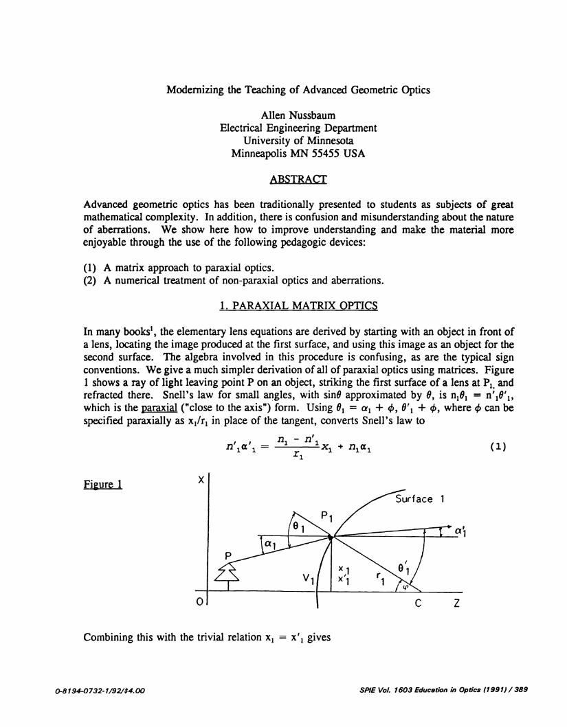
In many books' , the elementary lens equations are derived by starting with an object in front ofa lens, locating the image produced at the first surface, and using this image as an object for thesecond surface. The algebra involved in this procedure is confusing, as are the typical signconventions. We give a much simpler derivation of all of paraxial optics using matrices. Figure1 shows a ray of light leaving point P on an object, striking the first surface of a lens at P1 andrefracted there. Snell's law for small angles, with sinO approximated by 0, is n101 = n'10'1,which is the paraxial ("close to the axis") form. Using O = a + 4, O' + 4, where 4 can bespecified paraxially as x1/r1 in place of the tangent, converts Snell's law to
Fjgure 1
Combining this with the trivial relation x1 = x'1 gives
(1)
O-8194-0732-1/92/$4.OO SPIE Vol. 1603 Education in Optics (1991) /389
= nl — fl'ln'1a'1 x +
x
1
0 C Z
where the translation matrix T21 is
(n'1a'1 (1 —k1'('n1a1x' )(o
(1 —k1R1=I
/ 1 O\(n'1a'1'\x2 ) = t'1/n'1 'A x'i )
(1 0T21 =
1
The equation which combines a refraction, a translation, and a second refraction is then
390 / SPIE VoL 1603 Education in Optics (1991)
(6)
(2)
where the constant k1 is the refracting power of surface 1 and is defined as k1 = (n'1 - n1)/r1.The square matrix is the refraction matrix R1 for surface 1 , written as
(3)
For the ray traveling from surface 1 to surface 2 (Figure 2), the distance from the axis becomes(again paraxially)
x2 = + t'1cc'1 (4)
Another approximation is to regard t'1 as being equal to the distance between the lens verticesV1 and V2. Combining this with another trivial identity a = a2 gives the matrix equation
Figure 2 x
P2
0 V2
.1
z
(5)
( n'c''i (ncct '2 2) R2 '2j R1
(4 Cl1
This process can obviously be extended to any number of refracting (or reflecting) surfaces.The product S21 of the three square matrices is the system matrix and is also written as
( b -a\R2 T21 R1 = -d c)
(8)
where the Gaussian constants a, b, c, and d can be obtained by combining the above equationsto obtain
kkt'1 2 I I gnl nl
and
kt' kt'b=1— 21, c=1— (10)nl nl
For an object at t and an image at t' , we can connect the initial and final rays with the equation
(n'2&2\ _ ( 1 o(b —a( 1 0'fna\ (11)" xl I
—(t'/n'2 1)—d c)(,t/fl1 i)' X I
where the three 2 x 2 matrices on the right-hand side combine as an object-image matrix S
b--- -anlg - (12)p 4-,-d+ c--4.
This matrix implies that the value of the magnification m = x'/x will depend on a1, which leadsto an imperfect image. This means the lower left-hand element in the matrix must vanish, so that
= d - ct/n1 (13)fl'2 b - at/n1
and, in addition, m = c - at'/n'2. The positions of the unit planes H and H', the locations forwhich object and image are identical, are found be letting m = 1. Then
= 1H n'2(c — 1)/a (14)
SPIE Vol. 1603 Education in Optics (1991)1 391
with a similar expression for l. The focal point F' is located by letting x' = 0, so that l' =n'2c/a, and similarly for l. The focal lengths f and f' are defined as the distances between therespective focal and unit points. It then follows that 1/a = f' = 4. Let a ray leave a point onthe axis at an angle a and emerge at an angle a'2. Since x = 0 at the starting point, then n'2a'2= n1aI/m, where a'2/a1 is the angular magnification j, so that = 1/rn in air. The respectivelocations of the object and image for unit angular magnification are the nodal points N and N'.The six points F, F', H, H', N, N' comprise the cardinal points. The equal angle conditionshows that the nodal point locations are
(n'2/n1) - b(15)
nl a
and
= C - (n1/n'2)(16)
n2 a
The sign conventions used (and summarized by O'Neill3) are mostly the familiar Cartesian rules;to these are added the stipulations that a surface opening to the right(left) has a positive(negative)curvature and that a reversal of direction due to a reflection reverses the index.
The power of paraxial matrix optics is indicated by combining the definition of a, or 1/f' , in (9)with the definitions of k1 and k2 to obtain
which is the lensmakers' equation. This derivation is far more direct than usually found, andcan easily be extended to an arbitrary combination of components. As another example of theease of use of matrices, an object is 15 units to the left of a converging thin lens of focal length10 units. For such a lens, with t'1 negligable, (9) and (10) show that a = 1/f' , b = c = 1 , d= 0. A concave mirror, with radius of 16 units, is 20 units to the right of the lens. TheGaussian constants are then obtained by matrix multiplication. The cardinal points follow fromthe equations above, and are located to scale in Figure 3. We find the image by ray tracing.
Figure 3 II—.. 1+-• -+sf 4' Vy
392 / SPIE VoL 1603 Education in Optics (1991)
A ray from P is extended backwards to the unit plane H must then proceed to the right (thepositive direction) and parallel to the axis. The converse of this is a ray extended backwardsand parallel until it reaches H'; it then passes through F' and the two rays intersect at P'. Acheck is provided by a third ray from P to N; it emerges at N' and goes to P' while remainingparallel to its original direction. The values of t and t' shown are confirmed by the matrixcalculations. This situation can be readily extended to an arbitrary number of thick lenses.
Yet another example, and a truly remarkable one, is the Schwarzschild reflecting microscopeobjective, which has of two concentric mirrors of radii r1 = -(V'5 + 1) and r2 = -(V'5 + 1)(Figure 4). An object on the axis at a distance w = 1 from the common center will send aparallel beam up the tube. This may be confirmed by multiplying the two translation and tworefraction (actually, reflection) matrices involved and then using the fact that if the intitialposition and the final angle are zero, the upper left-hand corner of this product matrix mustvanish. Although this is a paraxial calculation, it is found that when the exact ray tracing isdone by the method given below, the angle of acceptance can be of the order of 25° (Figure 5).
Figure 4
When the paraxial approximation is no longer valid, then the concepts of Part 1 lose theirmeaning, and we can no longer use terms such as cardinal points, focal length, andmagnification. Instead, we must go to exact ray tracing. Figure 6 shows an object point P anda ray traveling to the first surface of a lens. A meridional ray leaves the object point P andstrikes surface 1 at the point P1. The translation is taken as a vector T1, direction cosines L, Mand N with respect to the x, y and z axes (note that OZ is taken as the symmetry axis). Thedirection cosines L and N are defined in terms of the components of T1 as
SPIE Vol. 1603 Education in Optics (1991) 1 393
Figure 5
2. MERIDIONAL NON-PARAXTAL OPTICS
L = T1X/T1, N= T1Z/T1 (18)
The location of the object point P and the intersection point P1 are also designated as vectors,and the three vectors shown in the figure are related by
R1=R+T1 (19)
Taking the dot or scalar product of each side with itself, we obtain
R = R2 + T + 2T1(zN + xL)
The equation of a circle in the coordinate system we are using may be written as
+ x = 2z1(r1 + v1)— v - 2v1r1 = R
Combining this with equation (20) and eliminating z1 gives
Using the curvature c1 = 1/r1, this quadratic equation becomes
T F1 —
-E + /E2 - c1F
where
E=3c1/2=c1[(z-v1)N+xL]-N (24)
Figure 6 x
CIz
nH
(20)
(21)
(22)
(23)
and
F= Cc1 = c1[(z-v1)2 + x2] — 2(z-v1) (25)
(Full details of the derivation have been given previously.) It is customary to shift the origin
394 / SPIE Vol. 1603 Education in Optics (1991)
after each translation, so that
and the other equation is
z + T1N —V1 (26)
x1 = x + T1L (27)
Since the angles or the direction cosines remain unchangedequations can be put into matrix form as
( n1N'1( 1
z1+v1)—
T1/n1 i) )
(n1L ( 1 n1L
x1)T1/n1 1)
during a translation, these two
(28)
and
(29)
The 2x2 matrix in these equations is the non-paraxial or exact translation matrix. The form ofthe exact refraction matrices can be obtained from Figure 7, which shows the incoming ray atsurface 1. This ray is taken to be a vector n1 with magnitude equal to the index of refraction onthe left. Then the refracted ray is designated as n1' in a similar way.
Figure 7
x
fl.1
0 z
Define a quantity K1, the refracting power or skew power, in terms of these two rays by therelation
= c1(n1 — fl'1)
where s1 is a unit normal vector at the surface. The scalar product of both sides of this equationwith this vector gives
(30)
SPIE Vol. 1603 Education in Optics (19911/395
K1 = c1(n cos0 - n1 cos01) (31)
We can express the scalar product of the incoming ray and the normal in two ways; these are
and
______ x1= + = n1N1 + n1L1—
= cos (1800 - 01) = -n1 cog
(32)
(33)
Combining these equations and using the direction cosines for the unit normal as indicated bythe figure, we obtain
cos 0 = N1(1 - c1z1) - L1x1c1 (34)
where z1 is measured from V1, as mentioned just above. Having foundcan find the angle after refraction with Snell's law, obtaining
K1 - Cl[flWi(flh/fl1i)2(1 - cos2 01) - n1cos 0]
Write (30) as the two scalar equations in matrix form
396 / SPIE VoL 1603 Education in Optics (1991)
the incident angle, we
(35)
nN-K1/c1 _ (1 -Ki'(fl1N1z;' (o iAZi
nL (1 -iç(n1L1x ¼0 lAxi
and
These equations show thatgeneralizations of the
Figure 8
(36)
(37)
the non-paraxial translation and refraction matrices arereduce for small
The procedure just developed has been applied to parallel meridional rays going through adouble convex lens with radii of 50 units, thickness of 15 units, and an index of 1.5. Thegraphics capability of the language QuickBASIC 4.5 is demonstrated by Figure 8, which showsthe pointdefect called spherical aberration, with the associated caustic surface and circle of leastconfusion. This figure emphasizes that spherical aberration isihe failure of meridional rays toobey the paraxial approximation, a definition unlike like what most optics books use'. Thisprogram has been extended5 to show how spherical aberration can be reduced by altering theradii while holding the thickness, index and focal length constant, a process called bending theLciis. It clearly demonstrates the advantage of numerical modeling, since the experiment cannotbe done on an optical bench.
3. NON-MERIDIONAL NON-PARAXIAL OPTICS
By adding a term yM to (24) and a term y2 to (25), as well as -M1L1c1 to (34), the abovemeridional procedure can be applied to non-meridional or skew rays. These changes imply theexistence of three translation and three refraction matrices, one pair for each of the corrdinates.A straightforward way of observing the aberration associated with skew rays is to consider acylinder of rays concentric to the axis and striking the first surface of a lens; it will form a sharpimage on axis somewhere to the left of the paraxial focus. Now incline this cyliner at an angleso that the rays strike the original circle on the surface, which means that the cyclinder will havean elliptical cross-section. The top and bottom rays, which are meridional, will define an imageplane. All the other rays, which are skew, will produce two approximately circular images, notquite coincident. This effect can be demonstrated using the ray tracing procedure just developedand is shown in Figure 9. One circle in each pair is produced by incident rays covering either
Figure 9 Figure 10
the left-hand or the right-hand half of the circle on the first surface of the lens. The combinationof the two image patterns produces cardiod patterns, as shown in Figure 10, which representscoma as it should occur for an uncorrected system. Hence, we define coma--in parallel with ourdefinition of spherical aberration--as the failure of skew rays to obey the paraxial approximation.This definition contradicts the customary one' and the patterns of Figure 10 are not found in thestandard texts. However, this effect is known to professional photographers6. Let us now
SPIE Vol. 1603 Education in Optics (1991)1397
assume that an optical system has been corrected both for spherical aberration and for coma.There is no guarantee that these separate corrections will bring the meridional rays and the skewrays from an off-axis point to a common focus. We thus see the source of astigmatism, whichis the failure of the two corrections to agree. This explains the classical illustration of thisaberration, found in all textbooks'. A meridional fan of rays leaving an off-axis object pointforms a sharp image. A second fan, at right angles to the first one, then represents one whichis completely non-meridional (except for a single, central ray) and it also forms a sharp, butseparate, image. The blur between these two points would be eliminated if they could be madeidentical.
4. SECOND-ORDER ASPHERIC SURFACES
Aspheric surfaces have been regarded as beyond the scope of undergraduate optics courses, andthey are treated by Smith1 with complicated iterative procedures. Restricting ourselves tosecond-order surfaces (paraboloids, ellipsoids, and hyperboloids), the above procedure can beextended easily once more by replacing the equation of the sphere--the three-dimensional formof (21)-with the conic section equation in the form
C(x2+y2—Sz2) -z=O (38)
where C is the vertex curvature and S is a shape factor which is negative for ellipsoids (S = -1specifies a sphere), zero for paraboloids, and positive for hyperboloids. As a typical example,consider the design of an arc furnace composed of two parabolic mirrors of radius 100 units.The contaminating arc is at one focus and the sample to be heated is at the second focus, whichcan be placed at an arbitrary distance. The program which does the ray tracing is given belowas an appendix and Figure 11 shows the resulting graphics. All the other examples given in thispaper were handled with this program, or simplified versions for meridional or non-meridionalspherical surfaces.
Figure 11
/\IN\LN\t--/1'\tz>-
L—L—YL2"4'i#y///y//1.:—j\J\\\N1
\\cN;1\\\///
Other examples which students find interesting (and for which listings are available from theauthors) are a keyboard-interactive lens-bending program (Figure 12), the formation of a virtualimage by a double concave lens (Figure 13), and the Hubble Space Telescope (Figure 14); thisinstrument uses two hyperbolic mirrors, and its parameters were taken from a popular article.
1. W. J. Smith, Modem Optical Engineering, 2nded, McGraw-Hill mc, (1990)2. A. Nussbaum and R. J. Phillips, Contemporary Optics, PrenticeHall, (1976)3. E. L. O'Neill, Introduction to Statistical Optics, Addison-Wesley, (1963)4. A. Nussbaum, Advanced Geometrical Optics on a Programmable Pocket Calculator,Amer
J Phys 42, 351 (1979)5. A. Nussbaum, urse Notes for Optical System Design (Unpublished)6. B. Sherman, ptographs of Optical Aberratian, Modem Photography 3, 1 18 (1968)
ELO=-.810 X = 0: Y = 0: Z — 0Zl — Z: Xl = X: Ti = 0EL — ELO: EM = 0: EN — SQR(1 - EL * EL - EM * EN)FOR J — 1 TO 3zv = z - T(J)D — 1 — (S(J) + 1) *EN * ENE — C(J) * (X * EL + Y * EN - S(J) * ZV • EN) - ENF — C(J) * (X * X + Y * Y — S(J) • ZV * ZV) — 2 • ZVSD — F I (SQR(E * E - D * F • C(J)) - E)x — x + SD * ELY = Y + SD * EMz — z + SD * EN — T(J)Ti = Ti + T(J)Z2 = Z 9- Ti: X2 = X
LINE (Zi, X1)—(Z2, X2), 9zi — Z2: Xi X2OP — 1 + S(J) * C(J) * ZSQ = SQR((X * X + Y * fl • C(J) * C(J) + OP * OP)COSTHETA — (EN * OP - C(J) * (EL * X + EM • Y)) / SQBC — N(J) * N(J) * (1 - COSTHETA * COSTHETA) I NP(J) I NP(J)KOVERC NP(J) * SQR(1 - BC) - N(J) * COSTHETAK — C(J) * KOVERCEL — (N(J) * EL - K * X / SQ) / NP(J)EM — (N(J) * EM - K * Y / SQ) / NP(J)EN (N(J) * EN + KOVERC * p / SQ) / NP(J)NEXT JELO ELO + .1IF ELO < .7 THEN 10
I Show mirrors
Ti — 0FOR Q = 1 TO 3Ti Ti + T(Q)X8 — 0: Z8 — TiFOR H — 1 TO 30X — X8 + 3: Z — X * X * C(Q) / (1 + SQR(C(Q) * C(Q) * S(Q) * X * X + 1))X9 X: Z9 — Z + TiLINE (Z8, X8)—(Z9, X9)X8 — X9: ZR — Z9NEXT HX8 — 0: Z8 — TiFOR H — 1 TO 30X — X8 — 3: Z = X * X * C(Q) / (1 + SQR(C(Q) * C(Q) * S(Q) * X * X + 1))X9 — X: Z9 — Z + TiLINE (18, X8)—(Z9, X9)X8 X9: Z8 — Z9NEXT HNEXT Q