N89 = 2094 8 EULER/NAVIER-STOKES CALCULATIONS OF TRANSONIC FLOW PAST FIXED- AND ROTARY-WING AIRCRAFT CONFIGURATIONSt J. E. Deese and R. K. Agarwal McDonnell Douglas Research Laboratories St. Louis, MO INTRODUCTION Computational fluid dynamics has an increasingly important role in the design and analysis of aircraft as computer hardware becomes faster and algorithms become more efficient. Progress is being made in two directions: more complex and realis- tic configurations are being treated and algorithms based on higher approximations to the complete Navier-Stokes equations are being developed. The obvious goal is the solution of complete aircraft flowfields with the full Navier-Stokes equations. The literature indicates that linear panel methods can model detailed, realistic aircraft geometries in flow regimes where this approximation is valid. Solutions for nonlinear potential equations for flowfields about nearly complete aircraft con- figurations have also been available for some time. Recently, Euler methods have progressed to the point of computing flowfield solutions for complete aircraft. As algorithms incorporating higher approximations to the Navier-Stokes equations are developed, computer resource requirements increase rapidly. Generation of suit- able grids becomes more difficult and the number of grid points required to resolve flow features of interest increases. Coupling greater grid density with the greater execution time per point needed to solve more complex equations creates requirements for large memory and long run-time. As a result, early work with the Euler and Navier-Stokes equations dealt with one- and two-dimensional flows or three- dimensional flow about simple geometries. Recently, the development of large vector computers has enabled researchers to attempt more complex geometries with Euler and Navier-Stokes algorithms. This paper describes the results of calculations for transonic flow about a typical transport and fighter wing-body configuration using thin-layer Navier-Stokes equations, and about helicopter rotor blades using both Euler/Navier-Stokes equa- tions. The two codes employed in the calculations have been developed at McDonnell Douglas Research Laboratories and are designated as MDTSL30 (thin-layer Navier- Stokes fixed wing-body code) and MDROTH (Euler/Navier-Stokesrotary-wing code). Both codes have been fully vectorized for optimum performance on a Cray supercom- puter. The codes have also been microtasked on a four-processor Cray X-MP/48 for reducing the wall-clock time by judicious use of various Cray software techniques. ?This research was conducted under the McDonnell Douglas Independent Research and Development program. PRECEDING PAGE BLANK NOT FlLlyEb 52 1 https://ntrs.nasa.gov/search.jsp?R=19890011577 2018-05-17T17:15:48+00:00Z
Transcript
N89 = 2094 8
EULER/NAVIER-STOKES CALCULATIONS OF TRANSONIC FLOW PAST FIXED- AND ROTARY-WING AIRCRAFT CONFIGURATIONSt
J. E. Deese and R. K. Agarwal McDonnell Douglas Research Laboratories
St. Louis, MO
INTRODUCTION
Computational fluid dynamics has an increasingly important role in the design and analysis of aircraft as computer hardware becomes faster and algorithms become more efficient. Progress is being made in two directions: more complex and realis- tic configurations are being treated and algorithms based on higher approximations to the complete Navier-Stokes equations are being developed. The obvious goal is the solution of complete aircraft flowfields with the full Navier-Stokes equations.
The literature indicates that linear panel methods can model detailed, realistic aircraft geometries in flow regimes where this approximation is valid. Solutions for nonlinear potential equations for flowfields about nearly complete aircraft con- figurations have also been available for some time. Recently, Euler methods have progressed to the point of computing flowfield solutions for complete aircraft.
As algorithms incorporating higher approximations to the Navier-Stokes equations are developed, computer resource requirements increase rapidly. Generation of suit- able grids becomes more difficult and the number of grid points required to resolve flow features of interest increases. Coupling greater grid density with the greater execution time per point needed to solve more complex equations creates requirements for large memory and long run-time. As a result, early work with the Euler and Navier-Stokes equations dealt with one- and two-dimensional flows or three- dimensional flow about simple geometries. Recently, the development of large vector computers has enabled researchers to attempt more complex geometries with Euler and Navier-Stokes algorithms.
This paper describes the results of calculations for transonic flow about a typical transport and fighter wing-body configuration using thin-layer Navier-Stokes equations, and about helicopter rotor blades using both Euler/Navier-Stokes equa- tions. The two codes employed in the calculations have been developed at McDonnell Douglas Research Laboratories and are designated as MDTSL30 (thin-layer Navier- Stokes fixed wing-body code) and MDROTH (Euler/Navier-Stokes rotary-wing code). Both codes have been fully vectorized for optimum performance on a Cray supercom- puter. The codes have also been microtasked on a four-processor Cray X-MP/48 for reducing the wall-clock time by judicious use of various Cray software techniques.
?This research was conducted under the McDonnell Douglas Independent Research and Development program.
The calculations presented in this paper have been performed on a Cray X-MP/48 Cray X-MP/14, Cray 2, or Convex C-2. Some of the results are presented in color- graphics form produced at a Silicon Graphics IRIS 2400T work station.
COMPUTATION OF WING/BODY FLOWFIELDS
Transonic flowfields about wing/body configurations are calculated by use of both the Euler and the Navier-Stokes equations. A code designated MDTSL30 has been developed at McDonnell Douglas Research Laboratories to compute flowfields by solv- ing the Euler, thin-layer, or slender-layer approximations to the Navier-Stokes equations.
The thin-layer approximation retains viscous terms in one direction. For high- Reynolds-number turbulent flow, the dominant viscous effects are the result of dif- fusion normal to a body surface. The thin-layer approximation is then suitable for geometries where the body can be mapped onto a single plane in the computational space, retaining viscous terms normal to this plane. A typical example is an
I isolated wing or fuselage.
The slender-layer approximation retains viscous terms in two directions, neg- lecting only streamwise terms. This approximation is useful for calculating viscous flows in regions where two aerodynamic surfaces interact, such as the wing-body
surfaces can be modeled with the slender-layer approximation. I junction or the wing-tip region. Viscous effects on both the fuselage and wing
The MDTSL30 code computes the turbulent flowfield by solving the three- I dimensional, Reynolds-averaged, thin-layer, or slender-layer approximation to the
Navier-Stokes equations on body-conforming, curvilinear grids. These equations are solved by employing Jameson's finite-volume explicit Runge-Kutta time-stepping scheme. viscosity model.
Turbulent effects are modeled by employing the Baldwin-Lomax algebraic eddy
The details of the methodology and the test calculations performed to verify the code are described by Deese and Agarwa1,l Agarwal, Deese, and Underwood,2 and Agarwal and D e e ~ e . ~ tools as described by Booth and Misegades.4
Microtasking was achieved by employing various Cray software
, Calculations have been performed for three different configurations: (1) the ONERA-M6 wing, (2) a typical transport wing-body configuration, and (3) a typical fighter wing-body configuration.
ONERA-M6 Wing: b = O . 84, a=3.Oo , Rec=ll . 7x10⁶ This standard test case was run on a mesh that had 192 cells wrapped around the
wing, 32 cells normal to the wing surface and 36 cells in the spanwise direction. There were 136 cells on the wing surface in the wrap-around direction and 24 on the
at the center of wing surface in the spanwise direction. the first cell was approximately four with about ten cells in the boundary-layer. The grid was constructed by stacking 2-D sectional grids along the wing-span. 2-D sectional grids were generated using the MDRL algebraic grid generation code.
m P
The value of y+ =
The
I 522
Figure 1 compares pressure distributions on the wing at five span stations as predicted using the Euler and thin-layer models. is good in the leading edge and trailing edge region. Shock smearing is greater than desirable, but can be attributed to the size of the cells in the mid-chord region. Cell width is typically 2-3% of the chord in this area with shocks being smeared over three or four cells. More grid points in the wraparound direction or a better distribution with less clustering in the leading- and trailing-edge regions would produce sharper shocks.
Agreement with experimental data5
C P
-1.25 -1 .00 -0.75 -0.50 -0.25
0 0.25 0.50 0.75 1 1.00 ' 1
-1.25 -1 .00 -0.75 -0.50
c -0.25 0
0.25
P
C P
0.50 1 0.75 I i 1.00 I 1
-1.25 -1 .00 -0.75
-0.50 -0.25
0 0.25
0.75 OSO I 1.00 ' 1
0 0.1 0.2 0.3 0.4 0.5 0.6 0.7 0.8 0.9 1.0
x/C
Experimentaldata Elder _----_-_-_-_-
- Thin-layer
t
0 0.1 0.2 0.3 0.4 0.5 0.6 0.7 0.8 0.9 1.0
X/C
Figure 1. Pressure distributions on an ONERA-M6 wing at various spanwise stations; Moo = 0.84, (Y = 3.0°, Re,= 11.7 X lo6, 192 x 32 x 36 mesh.
523
The thin-layer model produces a more accurate prediction of the wing pressure distribution than the Euler model. is too far downstream when the Euler model is used. The thin-layer model, which includes the effects of the boundary layer, capturesdshock location and strength more accurately.
Shock strength is too large and shock position
This case was also run on a smaller 140x48~32 grid on a four processor X-MP/48 to demonstrate the microtasking capability. megaword capacity of the machine. runtime using the microtasked version of the code was one hour on each of the four available processors for a total CPU time of four hours. approximately four orders of magnitude in 2500 iterations at a Courant-Friedrichs- Levy (CFL) number of 0.9. The actual speedup in wall-clock time of 3.73 achieved by microtasking is very close to the theoretical maximum of 3.77 as determined by Amdahl's Law.
The grid was limited by the eight Table I gives a summary of the results. Total
The residuals dropped
Table I. Performance evaluation of transonic viscous wing code MDTSL 30 on Cray X-MP/48.
4 0 Actual speedup achieved after microtasking = 3.73
0 Processing rate on 4-processorr: 6.3 x10⁴ wall clock secondsfmesh
0 Total CPU b e of microtasked aide is 5% less than original code
0 Number of iterations N = 2500
0 Root-mean-square residual at N = 1 is 0.106 xld
0 Root-mean-square residual at N = 2500 is 0.4830
point/ikXatiion
0 Reductionfcycle = 0.997
Total Cpu time = 14400.00 s
Transport Wing-Body: &=O. 76, a=2', Rec=6.4x10⁶
The grid lines on the surface of a typical transport wing-body configuration are
There
The value of y+ at the center of the first cell along the wing surface ranges
shown in Figure 2. configuration was generated with the 3-D grid-generation code of Chen et a1.6 are 96 cells on the wing in the chordwise direction and 34 in the spanwise direc- tion. from 1.5 to 3 while the value of y+ at the center of the first cell along the fuse- lage surface varies from 1.0 to 2.5.
A 160(chordwise)x34(wing-nonnal)x42(spanwise) mesh for this
524
m r J R L PAGE V’HbTOGRAPH
Figure 2. Typical transport configuration with surface grid lines.
Figure 3 shows the pressure distribution at five spanwise locations on the wing computed with the Euler and thin-layer Navier-Stokes codes and their comparison with experimental data. cluded in the calculations. As in the case of the ONERA-M6, the effect of including the thin-layer terms is to weaken shocks on the wing upper surface, move them for- ward, and improve the comparison with experimental data.
Thin-layer terms over the wing and the fuselage have been in-
A comparison of the slender-layer pressure distributions with thin-layer cal-
The major effect of culations and experimental data are shown in Figure 4. difference between the pressure distributions over the wing. including slender-layer terms should be near the wing-fuselage junction. mental data was available for comparison in this region.
As expected there is little
No experi-
Figure 5 shows pressure contours on the upper surface of the transport wing-body as displayed on an IRIS color graphics workstation. The location of the shock on the upper surface can be clearly identified.
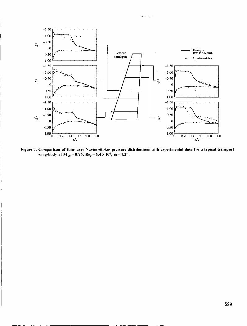
Thin-layer calculations were performed for the transport wing-body at an angle- of-attack of 4.2’. fuselage to reduce run time, so a 160x34~32 cell grid was used with clustering only near the wing surface. The value of y+ at the center of the first cell ranges from 1.5 to 3.0.
Navier-Stokes terms were included over the wing but not the
At this angle of attack, a significant region of separated flow appeared on the upper surface of the wing. wing surface. The separated flow region runs from about 30% of the local chord to the trailing edge starting at about 40% of the span and continuing to near the 80% span station.
Figure 6 shows the streamwise velocity just above the
Computed pressure distributions are compared with experimental data for five spanwise locations in Fig. 7. Near the fuselage and near the wing-tip the predic- tions compare well with experimental data. In the separated flow region the code
525
0.50 I/
- 4.50 CP
0.50 1.00 L
CP
-1.50 r. I
-1.00
4.50
0
0.50
1.00 - 0 0.2 0.4 0.6 0.8 1.0
X/C
Percent sefisp/4 - Thin-layer - Euler - Expenmental data
0.50 1 .00 L 4.50
- CP
0.50
Figure 3. Comparison of Euler and thin-layer Navier-Stokes pressure distributions with experimental data for a typical transport wing-body at M, = 0.76, Re, = 6.4 x 10⁶, (Y = 2.0°, 160 x 34 x 42 mesh.
1.00' ' ' ' ' ' ' ' ' . ' -1.50 r-----l
n Percent semispan
- Slender-layer ...______ nin- layer
ExperimentalData
-1.50
-1.00 4.50 mr/!/ ..
0
0.50
CP
1.00' ' ' ' ' ' ' ' ' ' ' 0 0.2 0.4 0.6 0.8 1.0
X/C
0.50 y 1.00' ' ' . ' ' ' ' ' ' '
- CP
xlc
Figure 4. Comparison of slender-layer and thin-layer Navier-Stokes pressure distributions with experimental data for a typical transport wing-body at M, = 0.76, Re, =6.4 X 10⁶, (Y = 2.0'. 160 x 34 x 42 mesh.
526
Figure 5. Pressure distribution, PIP,, on the upper surface of a typical transport wing-body, M, =0.76, Re, = 6.4 x lo6, a = 2.0".
predicts the shock to be too far downstream and stronger than was found experimen- tally. This result is consistent with experience using the Baldwin-Lomax turbulence models for transonic airfoil calculations under separated flow conditions.
A color contour map of the wing-body upper surface pressure is shown in Fig. 8. Again the shock location is clearly defined.
The grid lines on the surface of a typical fighter wing-body configuration are shown in Fig. 9. et a1.6 The grid has 144 cells in the chordwise direction, 34 cells normal to the wing, and 32 cells in the spanwise direction. wing have been included for this configuration so there is no grid clustering near the fuselage to accommodate viscous effects. in the chordwise direction and 24 in the spanwise direction. center of first cell along the wing surface ranges from 1.0 to 3.0.
The mesh was generated using the 3-D grid-generation code of Chen
Only the thin-layer terms near the
There are 96 cells on the wing surface The value of y+ at the
Figure 10 shows the pressure distribution at five spanwise locations on the wing computed with the Euler and thin-layer Navier-Stokes codes and their comparison with experimental data. Again the viscous effects tend to weaken the wing upper surface
527
ORIGINAL PAGE COI
Figure 6. Velocity contours, u / G , on the upper surface of a typical transport wing-body at M, = 0.76, Re, = 6.4 x 10⁶, and CY = 4.2'.
shocks and move them forward, although the effect is less pronounced for this configuration than for the transport wing-body discussed earlier.
Pressure contours on the upper surface of the fighter wing-body are displayed in Fig. 11.
COMPUTATION OF HELICOPTER ROTOR FLOWFIELDS IN HOVER AND FORWARD FLIGHT
An EulerlNavier-Stokes code, designated MDROTH, has been developed at McDonnell Douglas Research Laboratories for calculating the transonic flowfield of a multibladed helicopter rotor in hover and forward flight.
The code solves the three-dimensional Euler or Navier-Stokes equations in a rotating coordinate system on body-conforming curvilinear grids around the blades. The equations are recast in absolute-flow variables so that the absolute flow in the far field is uniform, but the relative flow is non-uniform. for the absolute-f low variables by employing Jameson's f inite-volume explicit Runge- Kutta time-stepping scheme. Rotor wake effects are modeled in the form of a correc- tion applied to the geometric angle-of-attack along the blades.
7. Comparison of thin-layer Navier-Stokes pressure distributions with experimental data for a typical transport wing-body at M, = 0.76, Re, = 6.4 x lo6, a= 4.2".
529
I
ORIGINAL PAGE COLOR PHOTOGRAPI
Figure 8. Pressure contours, PIP,, on the upper surface of a typical transport at M, =0.76, Re, = 6.4 x 10⁶, and a = 4.2'.
Figure 9. Typical fighter configuration with surface grid lines.
OSO 1 .oo L -1.50 I
OSO 1.00 u -1.501 . . . . . . . ' . I
CP
-1.00
-0.50
0
0 Experimentaldata Euler _______._._._
- Thin-layer
. CP
OSO 1 .oo I 0 0.2 0.4 0.6 0.8 1.0
X/C
0.50
1 .oo
0 w OSO 1 .oo 1
I
I
0.50 1 4 1 .oo u
0 - CP
OSO 1 .oo i 0 0.2 0.4 0.6 0.8 1.0
Figure 10. Comparison of Euler and thin-layer Navier-Stokes pressure distributions with experimental data for a typical fighter aircraft wing-body at M, = 0.90, Re, = 5.4 X lo6, a= 4.8", 144 x 34 x 32 mesh.
OAIQ(NAl PAGE Is OF POOR QUALW
53 1
ORIGINAL PAGE
Figure 11. Pressure contours, PIP,, on the upper surface of a typical fighter configuration; M, = 0.9, Re, = 5.4 x 10⁶, a = 4.8".
obtained by computing the local induced downwash with a free-wake analysis program. The details of the methodology are described by Agarwal and D e e ~ e . ~ - ~
A set of test calculations was performed by Agarwal and D e e ~ e ~ - ~ to verify the code for a model rotor in hover and forward flight at various collective pitch angles. The model rotor has two, untwisted, untapered blades of aspect ratio equal to six and a NACA 0012 airfoil section. formed by Caradonna and TunglO at NASA Ames Research Center for a range of blade tip Mach numbers, Mt, and collective pitch angles, 8,.
Experiments on this rotor have been per-
Like MDTSL30, the MDROTH code has been fully vectorized for optimum performance on a single-processor Cray X-MP and microtasked on a four-processor Cray X-MP/48 to reduce the wall-clock time by judicious use of Cray software techniques (Booth and Misegades4). The actual speedup in wall-clock time achieved by microtasking (3.73) is very close to the theoretical speedup possible (3.77), as was the case for MDTSL30.
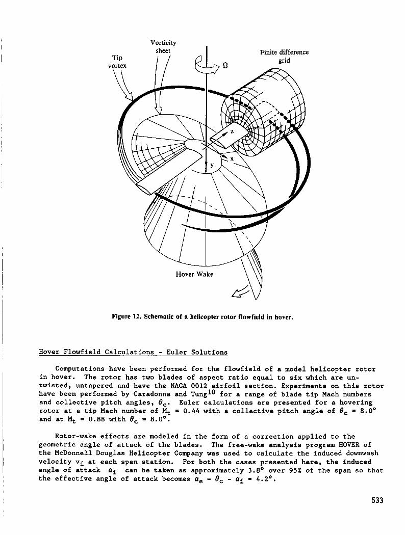
Figure 12 shows the main features of the flowfield of a two-bladed rotor in hover, with the imbedded finite-difference grid and the coordinate system. The flowfield is characterized by transonic shocks, complex vortical wakes, and blade- vortex interactions.
532
Vorticity I
Figure 12. Schematic of a helicopter rotor flowfield in hover.
Hover Flowfield Calculations - Euler Solutions Computations have been performed for the flowfield of a model helicopter rotor
in hover. twisted, untapered and have the NACA 0012 airfoil section. Experiments on this rotor have been performed by Caradonna and TunglO for a range of blade tip Mach numbers and collective pitch angles, 8,. Euler calculations are presented for a hovering rotor at a tip Mach number of Mt = 0 . 4 4 with a collective pitch angle of Bc = 8.0' and at Mt = 0.88 with Bc = 8.0'.
The rotor has two blades of aspect ratio equal to six which are un-
Rotor-wake effects are modeled in the form of a correction applied to the geometric angle of attack of the blades. the McDonnell Douglas Helicopter Company was used to calculate the induced downwash velocity vi at each span station. angle of attack ai the effective angle of attack becomes a, = Bc - ai = 4.2'.
The free-wake analysis program HOVER of
For both the cases presented here, the induced can be taken as approximately 3.8' over 95% of the span so that
533
These computations were performed on a 98(chordwise)x33(blade-normal) x2l(spanwise) mesh. A typical computation requires two million words of main memory, and 2.1*10-5 seconds of CPU time per mesh point for each iteration. converged solution required approximately six minutes of CPU time on a single processor of Cray X-MP/48 using the fully vectorized version of MDROTH.
A
Comparisons of computed pressure distributions with experimental data (Caradonna and TunglO) are shown in Fig. 13 for a hovering rotor at a tip Mach number of Mt = 0.44 and collective pitch angle 8, = 8', and in Fig. 14 for Mt = 0.88 and col- lective pitch angle 8, = 8'. Both cases indicate good agreement; further improve- ment can be achieved by refining the wake model.
Hover Flowfield Calculations - Navier-Stokes Solutions Navier-Stokes calculations for the model helicopter rotor in hover have been
performed at Mt = 0.44, BC = 8.0' and Mt = 0.61 and 8, = 8.0'. grid clustering near the blade surface was used to resolve the viscous layer. The effective angle of attack is 4.2' for both cases.
A 97x33~33 mesh with
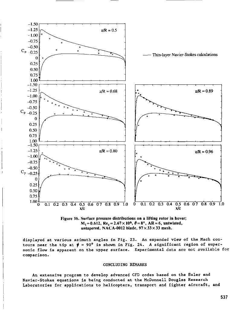
Figure 15 shows pressure distributions for the Mt = 0.44 case, while Mt = 0.61 results are presented in Fig. 16. Including the viscous effects had little effect on the surface pressure for those two cases. comparison.
No other data are available for
Forward Flight Flowfield Calculations - Euler Solutions Forward flight calculations have been performed for the model NACA 0012 rotor,
the OLS rotor, the MDHC 500E rotor, and the AH-64 Apache rotor. All forward flight computations have been performed on a 97x33~33 mesh. A typical calculation for the full rotor cycle from f=O' to f=36Oo requires 12 to 16 hours of CPU time on a Cray X-MP/14; approximately 80 iterations are required for one degree movement in the azimuth direction. The code is run in time-accurate mode starting with $=O and freestream conditions.
Figures 17 and 18 show a comparison of the computed pressure distributions on the model helicopter rotor in forward flight with experimental datalo for a location near the blade tip, and
(a) tip Mach number Mt = 0.7, advance ratio p = 0 . 3 , and collective rotor pitch angle ec=oo ,
I (d) tip Mach number Mt=0.8, advance ratio p=0.2, and collective rotor pitch angle OC=Oo, respectively.
In both cases, the computed results show good agreement with the experimental data.
Computations were performed for the OLS rotor blade at Mt = 0.63, p = 0.30 and a collective pitch angle 8, = 0. CAMRAD were used to determine the effective angles-of-attack along the OLS rotor blade at various azimuth angles. Pressure distributions computed with the Euler code are compared with inflight data at the 95X span station as shown in Fig. 19.
Results from the NASA Ames Research Center code
I I The calculations show good agreement with the experimental data.
I 534
- 1.5 I I I I I 1 - 1 . 5 I I I I I 1
- 3
- 1.5 I 1 I I
b z/R = 0.96
- 1 . 5 I I I I I I
- 1.0
- 0.5
CP 0
0.5
1.0 2 - 1.5 I I I 1 1 1
- 1.0
- 0.5
0 CP
0.5
I
Experimental data
untwisted, untapeied, NACA 0012 blade, 97 x 33 x 21 mesh. 0 0 Experimental data
0 0.2 0.4 0.6 0.8 1 .o x/c
Figure 13. Surface pressure distributions on a lifting rotor in hover: M, = 0.4, 8,= go, AR = 6, untwisted, untapered, NACA 0012 blade, 97 x 33 x 21 mesh.
0 0.2 0.4 0.6 0.8 1 .o x/c
Figure 14. Surface pressure distributions on a lifting rotor in hover; M, = 0.88 , 8, =go, AR = 6.0,
535
-1.5 I I I I 1 I I I I z/R = 0.50
0.5 - -
1 .o I I I I I I I I -1.5 I I I I I I I -
z/R = 0.68
-1.0
-0.5 C
0.5
1 .o I I I I I I -1.5 I I I I I I I 1
z/R = 0.80
P C
i n I I I I I A ...
0 0.2 0.4 0.6 0.8 1 .o x/C
-
U
Thin-layer Navier-Stokes calculations (with uniform wake correction along the blade, a&= 4.2')
Experimental data
I I I I - I I I I I I I 1 -
z/R = 0.96 .
X/C
Figure 15. Surface pressure distribution on a lifting rotor in hover: M, = 0.44, Re,= 2 x lo6, 8, = 8 O , AR = 6.0, untwisted, untapered, NACA-0012 blade, 97 x 33 x 33 mesh.
Figure 20 shows the pressure distribution, using the Euler code, computed on the 500-E rotor blade for a location near the blade tip. The calculation was performed for Mt = 0.58, p = 0.312, and Bc = 0' using effective angles-of-attack given by CAMRAD. Mach number contours on the blade upper surface at various rotor angles are shown in Fig. 21. No experimental data are available for this case.
The final forward flight results to be presented are for a helicopter rotor. Calculations were performed at a tip Mach number, Mt = 0.65 and p = 0.33. angles-of-attack were determined using 0. span station are shown in Fig. 22.
Effective Pressure distributions at the 95%
Mach contours on the blade upper surface are
536
-1.50 I
CP
-1.25 -1 .OO -0.75 4 . 5 0 4 .25
0 0.25 0.50 0.75 kI- 1 1.00 1
-1.50 I -1.25 -1 .00 -0.75 -0.50
'P -0.25 0
0.25 0.50 0.751 , , , , , , , , , 1 1 .oo
-1 S O -1.25 z/R = 0.80
-l*oo -0.75
0.50 0.75 i 1.00 L-
0 0.1 0.2 0.3 0.4 0.5 0.6 07 0.8 0.9 1.0 X/C
- Thin-layer Navier-Stokes calculations
1 z/R = 0.96
0 0.1 0.2 0.3 0.4 0.5 0.6 07 0.8 0.9 1.0 x/C
Figure 16. Surface pressure distributions on a lifting rotor in hover; M, = 0.612, Re, = 2.67 x lo6, 8 = 8 O , AR = 6, untwisted, untapered, NACA-0012 blade, 97 x 33 x 33 mesh.
displayed a t var ious azimuth angles i n Fig. 23. t ou r s near t h e t i p a t $ = 90' is shown i n Fig. 24. sonic flow is apparent on t h e upper sur face . comp ar is on.
An expanded view of t h e Mach con- A s i g n i f i c a n t region of super-
Experimental da ta are not ava i l ab le f o r
CONCLUDING REMARKS
An extens ive program t o develop advanced CFD codes based on t h e Euler and Navier-Stokes equat ions is being conducted at t h e McDonnell Douglas Research Laborator ies f o r app l i ca t ions t o he l i cop te r s , t r anspor t and f i g h t e r a i r c r a f t , and
53 7
-
y= 30"
Eula calculations 0 Experiment
-1.0
cP 1. O y= l5w pp x/C x/C
Figure 17. Pressure distribution on a model rotor-blade of NACA 0012 airfoil section and AR = 6 in forward flight; tip Mach number M, = 0.7, advance ratio p = 0.3, collective pitch 8, = 0, 96 x 32 x 32 mesh.
-1.0 I I 1 - Euler calculations 0 Experiment
Y = 30"
cP 0
Y'60" -l'k"u Y = 120" k?-.i 1 .o --
Y = W O CP 0
Y = 150"
0 0.5 -.05 0 0.5 4 C
1 .o -.05
XIC
Figure 18. Pressure distribution on a model rotor-blade of NACA 0012 airfoil section and aspect ratio 6 in forward flight; tip Mach number M, = 0.8, advance ratio p = 0.2, 96 x 32 x 32 mesh.
538
1 .00 -1.50
- - - -
0 Inflight data - Euler calculation - Full potential calculation -
-2.0 ""'F,,,,, 1 .00 I
-1.5
-1.0
cp 4 . 5
0
0.5
L O f I ' I I I I ' I I ' 0 0.1 0.2 0.3 0.4 0.5 0.6 0.7 0.8 0.9 1.0
xlc
0.501 -1.00
4.50
0
0.50
cP
0 0.1 0.2 0.3 0.4 0.5 0.6 0.7 0.8 0.9 1.0 X/C
Figure 19. Pressure distribution on the upper surface of the OLS rotor-blade in forward flight at 95% span location; tip Mach number M, = 0.63, advance ratio p = 0.30, collective pitch 6, = 0, 96 x 32 x 32 mesh.
539
P C
0.50 0.75
P C
.
.
-1.25 -1 .OO -0.75 -0.50 -0.25
0 0.25 0.50 0.75 1.00 ' 1
-1.25 -1 .00 -0.75 -0.50 -0.25
0 0.25 0.50 0.75
'. ..
Figure 20. Computed pressure distributions on the upper and lower surface of the MDHC 500E rotor-blade in forward flight at 95% span location; M, = 0.58, p = 0.312,96 x 32 x 32 cell mesh.
missiles and hypersonic vehicles. Representative calculations about a transport wing-body, a fighter wing-body, and a helicopter rotor clearly demonstrate that the state-of-the-art in CFD has progressed to the point that turbulent-flow calculations about complete fixed- and rotary-wing aircraft configurations may be achieved in the near future.
I Efficient use of large computers, including multiple-processor facilities, is receiving special attention.
540
ORIGINAL PAGE GouzFa: PHOTOGRAPH
Figure 21. Mach number contours on the upper surface of the 500E rotor-blade; M, = 0.58, p = 0.312.
ACKNOWLEDGMENTS
The authors would like to thank M. Uram of the McDonnell Douglas Aerospace Information Services Company for programming assistance and K. P. Misegades of Cray Research for microtasking the code for the Cray X-MP/48. like to thank D. Pritchard and D. S. JanakiRam of McDonnell Douglas Helicopter Company and N. L. Sankar of Georgia Institute of Technology for many useful discus- sions and assistance in various aspects of the rotor flowfield calculations. Some calculations were performed on the Cray Research X-MP/48, others were performed on the Numerical Aerodynamic Simulator. The authors gratefully acknowledge this assistance.
The authors would also
's .
-1.25 -1 .oo -0.75 -0.50
c -0.25 0
0.25
0.50 0.75 1 .oo
P
'4' = 30'
P C
-1.25 I -1 .oo -0.75 -0.50 -0.25
0 0.25 0.50
1 .oo
\y = 60"
P C
-1.25 -1 .oo -0.75 -0.50 -0.25
0 0.25 0.50 0.75
'f' = 90'
I
1.00 ' 1
0 0.1 0.2 0.3 0.4 0.5 0.6 0.7 0.8 0.9 1.0 X/C
1 Y = 150'
1 1
0 0.1 0.2 0.3 0.4 0.5 0.6 0.7 0.8 0.9 1.0 xic
Figure 22. Computed pressure distributions- on the upper and lower surface of a helicopter rotor-blade in forward flight at 95% span location; M, = 0.65, p = 0.33, 96 x 32 x 32 cell mesh.
542
ORIGINAL PAGE PHOTOGRAPH
Figure 23. Mach number contours on the upper surface of a helicopter rotor-blade; M, = 0.65 and p = 0.33.
543
Figure 24. Mach number contours on the upper surface of a helicopter rotor-blade; M, = 0.65, 1.1 = 0.33, and \k = 90'.
544
REFERENCES
1. Deese J.E. and Agarwal R.K. (1987), Navier-Stokes Calculations of Transonic Viscous Flow About Wing-Body Configurations, AIAA paper 87-1200, AIAA 19th Fluid Dynamics, Plasma Dynamics, and Laser Conference, Honolulu, Hawaii, June 1987.
2. Agarwal R.K. and Deese J.E., and Underwood R.R. (1985), Computation of Transonic Viscous Wing-Body Flowfields Using Unsteady Parabolized Navier- Stokes Equations, AIAA paper 85-1595, AIAA 17th Fluid Dynamics, Plasma Dynamics, and Laser Conference, Cincinnati, Ohio, June 1985.
3. Agarwal R.K. and Deese J.E. (1984), Computation of Viscous Airfoil, Inlet, and Wing Flowfields, AIAA paper 84-1551, AIAA 16th Fluid Dynamics, Plasma Dynamics, and Laser Conference, Snowmass, Colorado, June 1984.
4. Booth M. and Misegades K. (1986), Microtasking: A New Way to Harness Multiprocessors, Cray Channels, vol. 8, pp. 27-29.
5. Schmitt V. and Charpin F. (1973), Pressure Distributions on the ONERA-M6 Wing at Transonic Mach Numbers, AGARD-AR-138, chapter B-1.
6. Chen L.T., Vassberg J.C., and Peavey C.C. (1984), A Transonic Wing-Body Flowfield Calculation with Improved Grid Topology and Shock-Point Operators, A I M paper 84-2157, AIAA 16th Fluid Dynamics, Plasma Dynamics, and Laser Conference, Snowmass, Colorado, June 1984.
7. Agarwal R.K. and Deese J.E. (1987), Euler Calculations for Flowfield of a Helicopter Rotor in Hover, J. Aircraft, vol. 24, pp. 231-238.
8. Agarwal R.K. and Deese J.E. (1987), An Euler Solver for Calculating the Flowfield of a Helicopter Rotor in Hover and Forward Flight, AIAA paper 87-1427, AIAA 19th Fluid Dynamics, Plasma Dynamics, and Laser Conference, Honolulu, Hawaii, 8-10 June, 1987.
9. Agarwal, R. K. and Deese, J. E. (1988), Navier-Stokes Calculatlons of the Flowfield of a Helicopter Rotor in Hover, AIAA paper 88-0106, AIAA 26th Aerospace Sciences Meeting, Reno, Nevada, January 1988.
10. Caradonna F.X. and Tung C. (1981), Experimental and Analytical Studies of a Model Helicopter Rotor in Hover, Vertica, vol. 5, pp. 149-161.


![Semtex.c [CVE-2013-2094] - A Linux Privelege Escalation](https://static.documents.pub/doc/80x56/58f23e4c1a28ab994a8b4607/semtexc-cve-2013-2094-a-linux-privelege-escalation.jpg)


