Page 1
N91-10313
Evaluation of Alternatives for Best-Fit
Paraboloid for Deformed Antenna Surfaces
Menahem Baruch
Faculty of Aerospace Engineering
Technion, Haifa 32000, Israel
and
Raphael T. Haftka
Department of Aerospace and Ocean Engineering
Virginia Polytechnic Institute and State University
Blacksburg, Virginia 24061
159
https://ntrs.nasa.gov/search.jsp?R=19910001000 2020-07-03T16:20:35+00:00Z
Page 2
Abstract
Paraboloid antenna surfaces suffer performance degradation due to structural deforma-
tion. A first step in the prediction of the performance degradation is to find the best-fit
paraboloid to the deformed surface. This paper examines the question of whether rigid
body translations perpendicular to the axis of the paraboloid should be included in the
search for the best-fit paraboloid. It is shown that if these translations are included the
problem is ill-conditioned, and small structural deformation can result in large transla-
tions of the best-fit paraboloid with respect to the original surface. The magnitude of
these translations then requires nonlinear analysis for finding the best-fit paraboloid. On
the other hand, if these translations are excluded, or if they are limited in magnitude, the
errors with respect to the restricted "not-so-best-fit" paraboloid can be much greater than
the errors with respect to the true best-fit paraboloid.
Introduction
Paraboloid antenna surfaces suffer performance degradation due to structural deforma-
tion. A first step in the prediction of the performance degradation is to find the best-fit
paraboloid to the deformed surface. The process of finding this best-fit paraboloid has
received some attention in the past, (e.g. Refs. 1,2) but there is no clear agreement on
a procedure that should be followed. In particular, questions that arise are whether it is
acceptable to change the focus length in choosing the best-fit paraboloid and which rigid
160
Page 3
body motions should be included in moving from the original paraboloid to the best-fit
one. The present paper attempts to shed some light on this second question.
The choice of rigid body modes to be considered is associated with ill-conditioning of
the numerical process of obtaining the best-fit paraboloid. If z denotes the paraboloid
axis symmetry, then the ill-conditioning is associated with translations in the x and y
directions. Because antenna surfaces are typically shallow paraboloids, finding x and y
translations required to move the original paraboloid to the best-fit one leads to an ill-
conditioned set of equations. It is possible to eliminate these translations by, for example,
setting them to be equal to the corresponding translations at the apex. However, it is not
clear how much is lost in terms of the root mean square (rms) surface error. This paper
shows that not including these translations can indeed result in substantial increase in
rms errors, but that to include them one must resort to complicated and costly nonlinear
calculations. This is demonstrated first by the simpler case of a best-fit parabola.
Best-Fit Parabola
The undeformed shape of the parabola is given as
Yl -- ax2
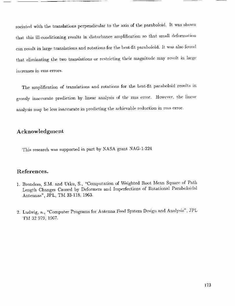
The distortions in the Xl and Ya directions are given by _ and r] (see Figure 1) so that
161
Page 4
a point A moves to position A'. The best-fit parabola is given as
Y = cx 2 (2a)
c--a+b (2b)
The two coordinate systems shown in Figure 1 have unit vectors ;1 and _1 associated with
the undeformed parabola, and ; and J: associated with the best-fit parabola.
The radius vector /_A from the apex of the original parabola to A / is given as
= + + + (3)
The closest point to W on the best-fit parabola is denoted B (Figure 1) and has the
coordinates [XB, (a + b)x2_] in the (x, y) coordinate system. The radius vector from the
origin of the original parabola to/3 is given as
"RB ---- tilT1 "4- _2]'1 + XB; 21- (a 31- b)X2B_ (4)
where /31 and/32 are the coordinates of the origin of the best-fit parabola. Denoting the
angle between the x, and x axes as/33 we have
71 -- 7 COS/33 -- _rsin/33
;2 = -_ sin/33 + _ cos/3a
(5a)
(Sb)
Using Eqs. (5) we can obtain from Eqs. (3) and (4) the error _ of A' with respect to the
best-fit parabola
(6)
162
Page 5
where (_A, YA), the coordinates of A' in the best-fit coordinate system are given as
"XA= (XA-4-_)COS/334-(ax2a-4-q)sin/33--/31cos/33--/32sin/33
"YA= --(XA+ _)sin/33+ (ax24+ r/)cos/33+/31sin/33--/32cos/33
(7a)
(7b)
-- !
The point/3 on the best-fit parabola is found by minimizing lIMB- RAIlwith respect
to x_. In the present work this is done with a Newton-Raphson iteration using XA as an
initial guess (XB is the solution to a cubic equation).
The parameters b,/31,/32,/33 are found by minimizing the root-mean-square (rms) dis-
tortion
n
i=1
where 4-h are the limits of the parabola, ci are quadrature weight and xi are points where
the deformed parabola coordinates are given. In this work the minimization was performed
by a conjugate-gradient method using finite-difference derivatives.
Instead of performing this nonlinear analysis it is standard practice to linearize the
problem. First we set cos/33 -- 1, sin/33 = /33 and neglect higher order terms in Eqs.
(7) (assuming _, r/ , /31, /32 , /33 are small) to get
"XA = X A 4" _ 4" aX2A/33 -- /31
-_A= --xA/33+ ax_ + _ --/32
(9a,)
(9b)
163
Page 6
Next we usea linear approximation to the minimum distanceasfollows: We set x B =
ZA in Eq. (6) and take only the component of _' normal to the best-fit parabola at
X B -- X A. This normal _ is given as
= y- 2(a+b)xA; (10)
1 + 4(a + b)2XA 2
Neglecting higher order terms the normal component of v can be written as
b'n -- /2 • n ---- --Po -3t- _TO/ (11)
where
and
Vo = (r/ - 2axA_)/V/1 + 4aZx 2
fT = [X2A,_2aXA, I,xa + 2a2X3A]/_/1 + 4a2X2A
(12)
(13)
The rms error is now defined as
2h
To minimize it we differentiate Eq. (14) with respect to ct to obtain
1 /h ooqOr"-v,_-_-.-dx = 02h h
Using Eq. (11), Eq. (15) becomes
Aa= f
j = 1, ...,4
(14)
(15)
(16)
164
Page 7
where
A= =h i=1
ff -- vogdx - CiVo(Xi)£(xi)h i=I
(17a)
(17b)
The matrix A is almost singular so that small deformations _, 7/ can result in large
values of/31 (the x-translation) and/33 (the rotation). We can minimize _']ms with an
additional limitation on the size of ct of the form
ara <_ ¢ (18)
and this leads to a system of equations
(A + Al)a = f (19)
where ,_ is a Lagrange multiplier (chosen to satisfy Eq. (18)) and I the identity matrix.
Best-Fit Paraboloid
The derivations for the paraboloid parallel the derivations for the parabola given in the
previous section.. The undeformed shape of the paraboloid is given as
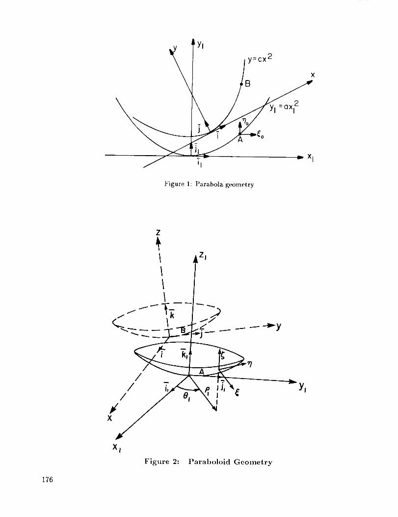
Z 1 = ap_ (20)
in a coordinate system shown in figure 2. The distortions in the ill, 01 and z 1 directions
are given by _, r/ and _, respectively, so that point A in Figure 2 moves to position A I.
165
Page 8
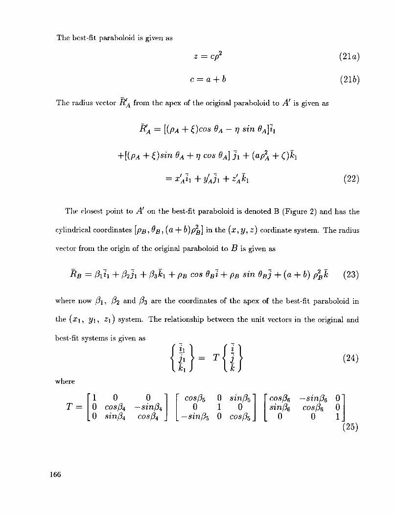
The best-fit paraboloid is given as
z "- cp 2 (21a)
c=a+b (21b)
--!
The radius vector R A from the apex of the original paraboloid to A I is given as
/_4 = [(IOA Jr- _)C08 0 A -- 7] 8ir_ OA]; 1
+[(PA + _)sin OA + 71COS OA] j1 _- (ap2A + _)k,
' - '- Z_4k I (22)= XAZl -Jr- YA31 -'F
The closest point to A' on the best-fit paraboloid is denoted B (Figure 2) and has the
cylindrical coordinates [PB, OB, (a nu b)p 2] in the (x, y, z) cordinate system. The radius
vector from the origin of the original paraboloid to B is given as
RB = _1;1 -1- _2jl nt- _3_1 nt- [B COS OB_ -nt- DB 8itl OBj -nt- (a --_ b) p2BfC (23)
where now t31, /32 and/33 are the coordinates of the apex of the best-fit paraboloid in
the (Xl, Yl, Zl) system. The relationship between the unit vectors in the original and
best-fit systems is given as
(24)
where
T
1 0 0
0 C08]_ 4 --sin�34
0 sinfl4 c0s/34
cos/3s 0 sinfls0 1 0
-sinfls 0 cos/3s"c0s/36-sin/36 !]
sin/36 c0s/360 0
(25)
166
Page 9
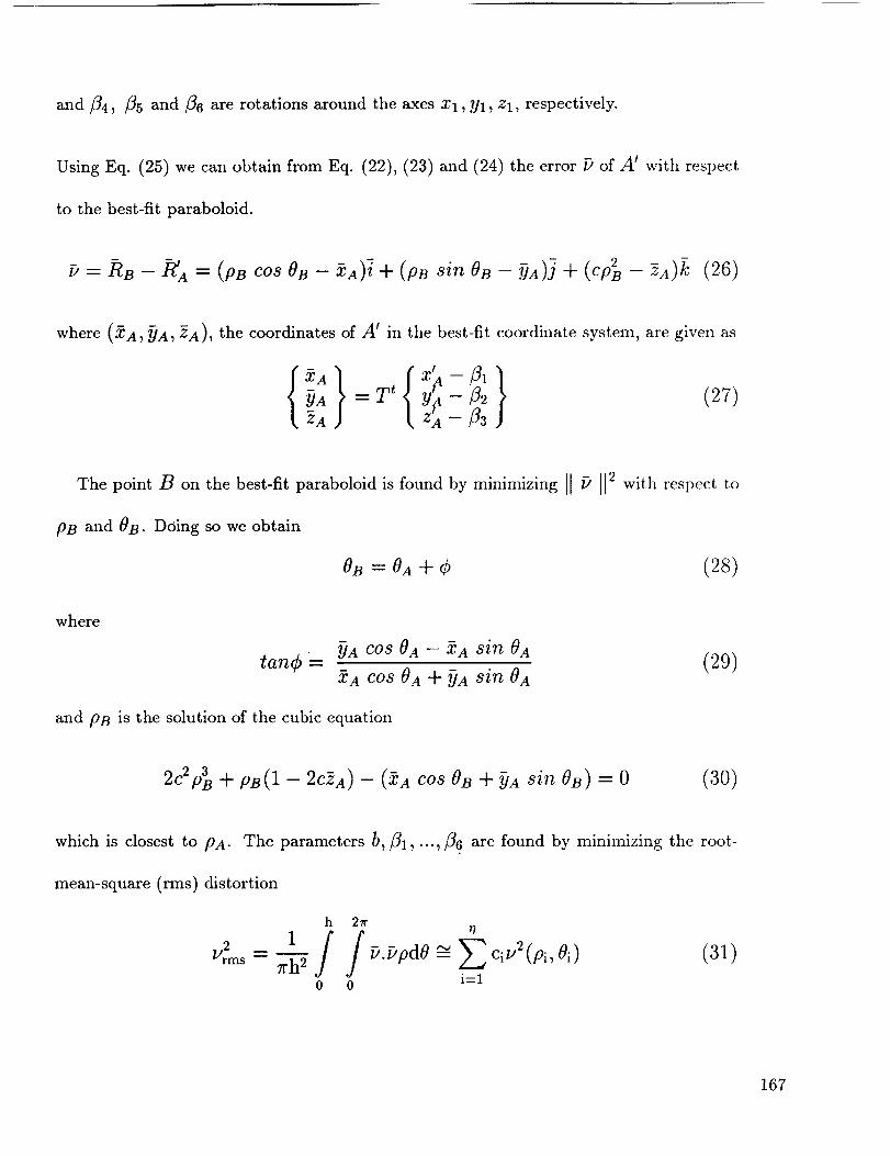
and f14, f15 and fl6 are rotations around the axes Xl, Yl, Zl, respectively.
Using Eq. (25) we can obtain from Eq. (22), (23) and (24) the error _ of A' with respect
to the best-fit paraboloid.
r.= i_, - i_'A= (.08coso, - _A)i+ (p, =ino, - f_A)j+ (cp_- _A)_(26)
where (5:A, YA, fi-A), the coordinates of A' in the best-fit coordinate system,
YA = T t Y f12ZA Z A _3
are given as
(27)
The point B on the best-fit paraboloid is found by minimizing _ 2 with respect to
pB and OB. Doing so we obtain
08= 0_+ ¢ (2s)
where
tan¢ = f]A C08 0 A -- XA sin OA (29)YeACOS OA + flA sin OA
and PB is the solution of the cubic equation
2cZp_ + pB(1 - 2C_A) -- (Y:a COS OB + flA sin 08) = 0 (30)
which is closest to PA. The parameters b,/_1, "", _6 are found by minimizing the root-
mean-square (rms) distortion
h 2_r
Vrms 7rh 2
0 0
7/
Z ci u 2 (Pi, 0i) (31)i=1
167
Page 10
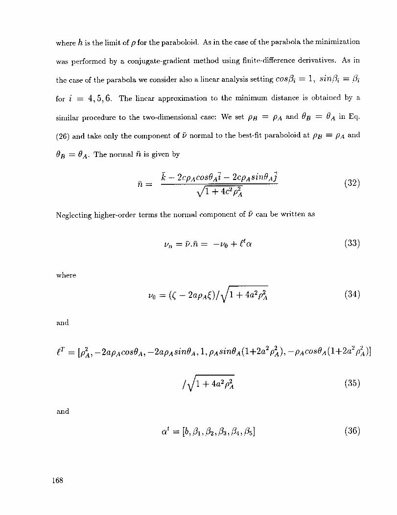
whereh is the limit of p for the paraboloid. As in the case of the parabola the minimization
was performed by a conjugate-gradient method using finite-difference derivatives. As in
the case of the parabola we consider also a linear analysis setting cos/3i = 1, sin/3i =/3i
for i = 4, 5, 6. The linear approximation to the minimum distance is obtained by a
similar procedure to the two-dimensional case: We set fib = flA and 0 B = 0 A in Eq.
(26) and take only the component of _ normal to the best-fit paraboloid at fib = flA and
OB = OA. The normal fi is given by
fi = k- 2CpACOSOA_-- 2CpASinOA_ (32)
X/1 + 4dp2A
Neglecting higher-order terms the normal component of _ can be written as
v,_ = u.n = -Yo + gtc_ (33)
where
and
_T _-[p2A,--2apAcosOA,
and
vo = (_ - 2apA_)/¢l + 4a2p2A (34)
--2apA sinOA, 1, pA SinOA ( I +2a2 p2A), --pAcOSOA (I + 2a2p2A)]
/V/1 + 4a2p2A (35)
C[t -- [b, ill,/32,/33,/34,/351 (36)
168
Page 11
Note that, as expected becauseof axial symmetry, r# and /36 do not influence the error.
The rms error is again defined as
h 21r
V;m.= 7fi-7o o
and the minimization again leads to a system of linear equations.
(37)
Ao_ = f (38)
whereh 2_r
n
A= ii'".'.'O : ECi'i(Di,Oi)':(pi, Oi) (39a)0 0 L=I
h 27rrl
0 0 L=I
(39b)
Results for Best-Fit Parabola
To illustrate the problems associated with finding the vector o_ which defines the best-fit
parabola consider a distortion of the form
27ex
-- _c(1 - cos --if-) (40)
with r/= 0. A parabola with a/h = 0.2 corresponding .to focal length over diameter ratio of
0.625 was used. The best-fit parabola was calculated for a very small disturbance _c/h =
0.005. The best-fit parabola corresponding to this distortion was calculated three different
ways:
169
Page 12
(i) By using conjugate gradient optimization procedure to minimize Ij2rns based on the
nonlinear expressions in Eqs. (6) and (8). The resulting surface error is denoted PNL.
(ii) By solving the linearized problem Eq. (16). The corresponding linear approximation to
the surface distortion is denoted VL.
(iii) By solving the size-limited problem, Eq. (19) for various values of )_.
The results are summarized in Table 1. The first line shows the results obtained with
conjugate gradient minimization of the nonlinear expression for the error. It is seen that
the rms value of the error can be reduced by a factor of three. However, there is great
amplification of the disturbance with the normalized translation /31/h being equal to
0.1571. The linear analysis based on Eq. (16) yielded similar values for the components
of oz. However, because of the large values of these components the prediction of that
linear analysis was erroneous. The predicted rms value of 4.9 x 10 -4 compares with a
nonlinear value of 6.37 x 10 -3. Thus while the linear analysis predicted a reduction of
the initial rms by a factor of 3 the nonlinear analysis predicted that the best-fit linear
parabola actually increased the error by a factor of three and a half.
The next three lines in Table 1 include size-limited solutions obtained from Eq. (19)
with various values of/_. It is seen that as )_ is increased the size of oz decreases so that
the linear and nonlinear predictions become close. However, this is accompanied with
substantial increase in the best-fit rms error. The last line in the table shows a 3-variable
170
Page 13
solution obtained by setting fll to the apex x-translation (zero here). This solution is close
to the large-,_ solution from Eq. (19).
Table 1 shows that we have a dilemma in the construction of a best-fit parabola. Linear
analysis requires that we eliminate one of the variables or restrict the size of the solution.
These limitations, however, substantially increase the error rms of the now 'not-so-best-fit'
parabola. The alternative nonlinear solution is complex and costly.
This type of difficulty is not encountered when the distortion does not require fil and
f13 for its correction. As an example consider a distortion of the form
27rx
{ = (41)
The results of the nonlinear and linear solutions are shown in Table 2 for a substantial
value of _s/h -- 0.04. It is seen that there is hardly any difference between the linear
and nonlinear solutions.
Results for Best-Fit Paraboloid.
Similar results were obtained for the best-fit paraboloid for a/h = 0.2. For example,
a distortion of the form
was considered,
= Gsin(Trp/h)sinO
and the results for _s/h = 0.001 are summarized in Table 3.
(42)
The first
column shows the results of the nonlinear analysis coupled with the conjugate gradient
171
Page 14
minimization. The rms error is reducedby about a factor of 7, however there is again
amplification of the distortion due to the ill-conditioning of the problem with/32/h =
0.09. The linear analysis shown in the secondcolumn produces very similar solution,
predicting evenbetter reduction in rms (about a factor of 10). However,whenthe nonlinear
solution is analyzedusingthe nonlinearanalysiswefind that the error actually increased
by a factor of 3.
The next three columns in Table 3 show the size-limited solutions based on Eq. (19). It
is seen that, as we put more and more stringent limits on the magnitude of the solution,
the agreement between the linear and nonlinear solution improves. However, much of the
reduction in the error is lost, so that we have a 'not-so-best-fit-paraboloid'. Similar results
are obtained by setting/31 and _2 equal to x and y translation of the apex (zero for the
example) and solving a reduced 4-variable problem.
While this dilemma of how to calculate the best-fit-paraboid is difficult, there is a bright
side to it. The linear analysis gives a reasonable idea of the magnitude of error reduction
possible with the best-fit paraboloid.
Concluding Remarks
An investigation of alternatives for calculating the best-fit paraboloid to a deformed
paraboloid surface was investigated. In particular we focused on the ill-conditioning as-
172
Page 15
sociated with the translations perpendicular to the axis of the paraboloid. It was shown
that this ill-conditioning results in disturbance amplification so that small deformation
can result in large translations and rotations for the best-fit paraboloid. It was also found
that eliminating the two translations or restricting their magnitude may result in large
increases in rms errors.
The amplification of translations and rotations for the best-fit paraboloid results in
grossly inaccurate prediction by linear analysis of the rms error. However, the linear
analysis may be less inaccurate in predicting the achievable reduction in rms error.
Acknowledgment
This research was supported in part by NASA grant NAG-I-224
References.
1. Brondess, S.M. and Utku, S., "Computation of Weighted Root Mean Squarc of Path
Length Changes Caused by Deformers and Imperfections of Rotational Paraboloidal
Antennas", JPL, TM 33-118, 1963.
2. Ludwig, a., "Computer Programs for Antenna Feed System Design and Analysis", JPL
TM 32-979, 1967.
173
Page 16
Table 1: Best-fit parabola with variousfitting schemes,_c/h - 0.005, initial error
Uo,.,,s/h = 1.75 x 10 -3
Fitting scheme b/h t_l/h /_2/h _3/h b'L/h I/NL/h
rms values
4-variable
nonlinear .00104 .1571 .00426 .05854 4.90 X 10 -4
linear 0. .1574 0. .05844 4.90×10 -4 6.37x10 -3
)_ -- .00001 0. .1238 0. .05844 4.90x 10 -4 3.90x 10 -3
)_ -- .0001 0. .0426 0. .0146 8.91 x 10 -4 9.74x 10 -4
)_ -- .0002 0. .0248 0. .00785 9.89x 10 -4 9.95x 10 -4
)_ -- .0005 0. .0113 0. .00267 1.07x 10 -3 1.07x 10 -3
3-variable 0. 0. 0. -.00163 1.13x 10 -3 1.13x 10 -3
Table 2:
8.69 x 10³
Best-fit parabola with various fitting schemes, _s/h -- 0.04, yo_ms/h -
Fitting scheme b/h /31/h t32/h
nonlincar .0142 0. -.00228
linear .0141 0. -.00225
fl3/h uL/h YNL/h
rms values
0. 6.02×10 -3
0. 5.69X 10 -3 6.02X 10 -3
174
Page 17
Table 3: Best-fit parabola with various fitting schemes,_s/h -- 0.001, initial error
yo,.ms/h = 4.868 x 10 -4
Fitting
scheme
nonlinear
6-variable 4-variable
linear
)_=5xlO-6A=2x10 -SA=5x 10 -sA=O
b/h 2.33x 10 -40. O. O. O. O.
fll/h O. O. O. O. O. O.
fl2/h -0.09055 -0.09055 -0.06281 -0.03280 -0.01686 O.
/33/h 1.41×10 -30. O. O. O. O.
/_4/h -0.03366 -0.03366 -0.02313 -0.01174 0.00569 7.12x 10 -'t
/3s/h o. o. o. o. o. o.
uL/h 5.19x10 -s 1.12xlO -4 2.14x 10 -4 2.70x 10 -4 3.29x 10 -'1
VNL/h 6.91X10 -5 1.47X10 -3 7.05X10 -4 2.79X10 -4 2.73x10 -4 3.29x10 -4
175
Page 18
Figure 1: Parabola geometry
X
XI
Figure 2: Parabolold Geometry
176
Page 19
SESSION 43 (W2)WORK-IN-PROGRESS II
177