18
1 Nagaoka 4D Seismic Revisited Naoshi Aoki, ○ Akihisa Takahashi , Kazuya Shiraishi, Takao Nibe (JGI, Inc.), Ziqiu Xue (RITE) 2011.6.7 IEAGHG 7th Monitoring Network Meeting
1
Nagaoka 4D Seismic Revisited
Naoshi Aoki, ○Akihisa Takahashi , Kazuya Shiraishi, Takao Nibe (JGI, Inc.),
Ziqiu Xue (RITE)2011.6.7
IEAGHG 7th Monitoring Network Meeting

2
From RITE Website
CO2 injection demonstration test was conducted by RITE at Nagaoka FY 2000-2004
Total amount of 10,405 tons of CO2 was injected.

3
4D Seismic Extent
1.7 km
2.0 km
4D
Seismic
Extent
and
Well
Locations
4D Seismic
IW-1OB-2
OB-3OB-4
Tanase et al. (2008)Well Locations
Depth Structure Map and
4D Seismic Extent

4
Injection History
Xue
et al. (2006)Red Square: CO2 Breakthrough at the well

5
2800m/s
2200m/s
Modified from Tanase
et al.(2008)
Pink and Green shows simplified velocities before and after CO2 breakthrough
Velocity Difference before/after CO2 breakthrough OB-2

6
Revisit the 4D seismic
• Time lapse seismic surveys were conducted in 2003 and 2005.
• Two surveys were reprocessed using the up‐ to‐date processing software.
• Seismic response in the five‐meter‐thick injected zone was re‐evaluated.
• Acoustic impedance inversion was conducted.

7Reprocessing Results 2005 Repeated Survey
Time Slice 1.006sec
IL82
East of the injection areais contaminated with
migration noises.
WNW ESE
500 m

8Reprocessing Results Time Slices (1.006sec)
Previous Processing Re-processing
S/N improvement around reservoir
2005 Monitoring survey500 m

9
Log‐Seismic Correlation
OB-2 OB-3 OB-4
Blue:Synthetic Seismogram Red:Seismic DataLog-seismic correlation is fairly good except for OB-2.
OB-2 location would be contaminated with migration noises.

10
Injected Zone and Seismic Resolution
OB-4 Acoustic Impedance
Ic:Zone2b4 msec (5 m)
λ=65 m(43 Hz)
Zone2_top
Zone3_top
Extracted Wavelet
Injected zone of 5 meters corresponds to 1/13 of wavelength
No separability but still have visibilityunder the good S/N ratio.
Blue: Actual AI Red: Estimated AI

11
11
OB-4 Synthetic Seismogram: Before CO2 arrival
Density Velocity AI REFC
SyntheticSeismogram
Bfr CO2 Arrival
SeismicSection
2005
Seismic IL82
1000 ms
950 ms

12
12
OB-4 Synthetic Seismogram: After CO2 arrival
Density Velocity AI REFC Seismic IL82
1000 ms
950 ms
• Travel timedifference is
just an 1 msec.
•Amplitude differencearound the target
is visible
SyntheticSeismogram
Aft CO2 Arrival
SeismicSection
2005
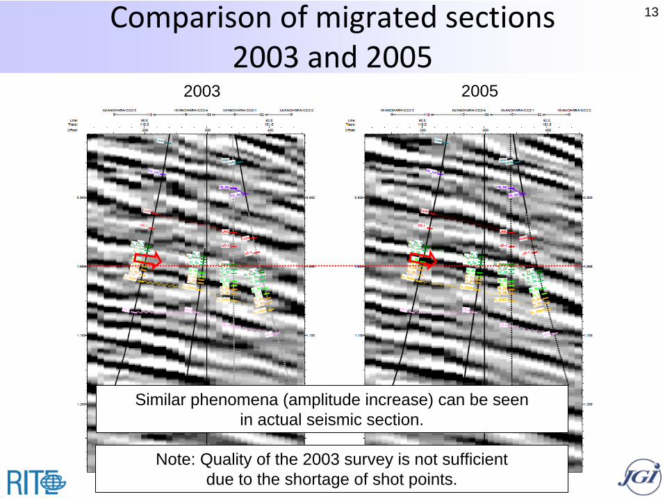
13Comparison
of
migrated
sections 2003
and
2005
20052003
Similar phenomena (amplitude increase) can be seenin actual seismic section.
Note: Quality of the 2003 survey is not sufficient due to the shortage of shot points.

14AI Inversion Results 2005 Survey
Low impedance anomaly is observed a bit below the injected zone in AI inversion.
OB-3(Projected)
OB-4 IW-1 OB-2 High
Low
Injected ZoneLow AI Anomaly
Lc Top
1000 ms
980 ms
1020 ms
1040 ms
15
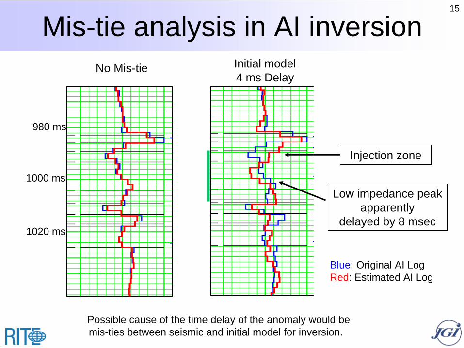
Mis-tie analysis in AI inversion No Mis-tie Initial model
4 ms Delay
Blue: Original AI Log Red: Estimated AI Log
Low impedance peak apparently
delayed by 8 msec
Injection zone
980 ms
1000 ms
1020 ms
Possible cause of the time delay of the anomaly would bemis-ties between seismic and initial model for inversion.

16Volume Attribute Average AI Value (2005 Survey)
Average AI Value (Lc top +6 to +26 msec)
Orange to Yellow: Low Impedance Area
OB-2
OB-3
OB-4

17
Summary of Results
• 4D response from such a thin layer (5 meters) can be detected.
• Quality of the 2003 survey was not sufficient for 4D processing due to the shortage of shot points.
• Extent of CO2 can be recognized by amplitude anomaly in the 2005 survey.
• Position of amplitude anomaly on AI inversion would be estimated a bit downward due to
mis‐ties.

18
Thank you for your kind attention
Evaluation of the Nagaoka test field is still ongoing.


