49
CMSC 858M/AMSC 698R Fast Multipole Methods Nail A. Gumerov & Ramani Duraiswami Lecture 13
CMSC 858M/AMSC 698R Fast Multipole Methods
Nail A. Gumerov & Ramani Duraiswami
Lecture 13
Outline • Data Structures and FMM • Hierarchical Space Subdivision
– Binary Trees, Quadtrees, Octrees; – k-d trees; – 2d-trees. Definitions.
• Hierarchical Numbering (Indexing) • Spatial Ordering
– Scaling. – Binary ordering. – Ordering in d-dimensions. – Bit interleaving and deinterleaving – Algorithms for finding the box index, box center, parents,
children, and neighbors. – Examples.
Data Structures and FMM
• Spatial grouping techniques are employed in various versions of the FMM (SL_FMM, RML_FMM, AML_FMM, etc.)
• All major components of the FMM are interrelated: truncated factorization, error bounds, translation operations, and spatial grouping.
Data Structures and FMM (2) • Since the complexity of FMM should not exceed O(N2) (at
M~N), data organization should be provided for efficient numbering, search, and operations with these data.
• Some naive approaches can utilize search algorithms that result in O(N2) complexity of the FMM (and so they kill the idea of the FMM).
• In d-dimensions O(NlogN) complexity for operations with data can be achieved.
• Some caution is needed while utilizing standard (library) routines on sets. If using such routines always check the complexity of the algorithm!
• Understanding of complexity of each FMM procedure is crucial. Normally it is worth to develop your own library for operations with FMM data (using standard routines as their complexity is satisfactory).
Data Structures and FMM (3) • Approaches include:
– Data preprocessing • Sorting • Building lists (such as neighbor lists): requires memory, potentially
can be avoided; • Building and storage of trees: requires memory, potentially can be
avoided; – Operations with data during the FMM algorithm
• Operations on data sets; • Search procedures.
• Preferable algorithms: – Avoid unnecessary memory usage; – Use fast (constant and logarithmic) search procedures; – Employ bitwise operations; – Can be parallelized.
Hierarchical Space Subdivision Historically: • Binary trees (1D), Quadtrees (2D), Octrees
(3D); • For dimensions larger than 3 (sometimes for
d=2 and 3 also) k-d trees. • We will consider a concept of 2d-tree:
– d=1 – binary; – d=2 – quadtree; – d=3 – octree; – d=4 – hexatree; – and so on..
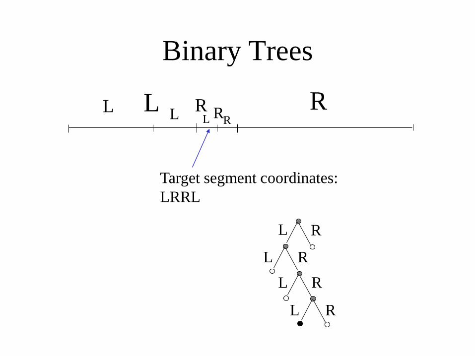
Binary Trees
L R L R L R L R
Target segment coordinates: LRRL
L R
L R L R
L R

What are k-d trees? Target box coordinates: RBRTLBRT
L R T
B L R T
B
R L T
B L R T B
R L B T
R L T B
R L
T B R L
T B
Like a binary tree!
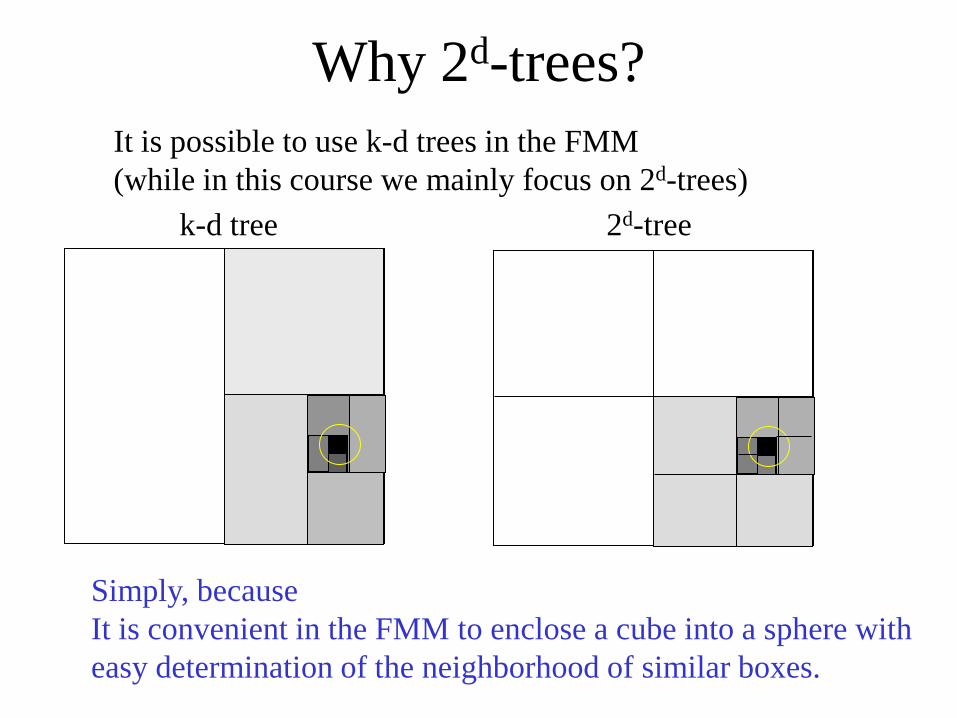
Why 2d-trees? It is possible to use k-d trees in the FMM (while in this course we mainly focus on 2d-trees)
Simply, because It is convenient in the FMM to enclose a cube into a sphere with easy determination of the neighborhood of similar boxes.
k-d tree 2d-tree
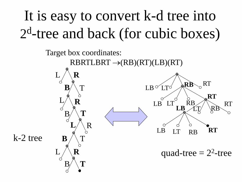
It is easy to convert k-d tree into 2d-tree and back (for cubic boxes)
Target box coordinates: RBRTLBRT →(RB)(RT)(LB)(RT)
R L B T
R L T B
R L
T B R L
T B
LB LT RB RT
LB LT RB RT
LB LT RB RT
LB LT RB RT
quad-tree = 22-tree k-2 tree
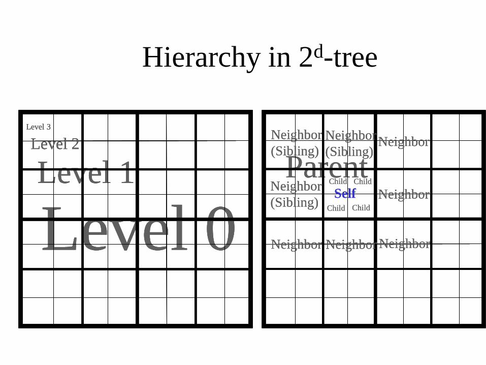
Hierarchy in 2d-tree
Level 1
Level 0 Level 2
Level 3
Parent Self
Child Child
Child Child
Neighbor (Sibling)
Neighbor Neighbor Neighbor
Neighbor
Neighbor Neighbor (Sibling)
Neighbor (Sibling)
Level 1
Level 0 Level 2
Level 3
Level 1
Level 0 Level 2
Level 3
Parent Self
Child Child
Child Child
Neighbor (Sibling)
Neighbor Neighbor Neighbor
Neighbor
Neighbor Neighbor (Sibling)
Neighbor (Sibling)
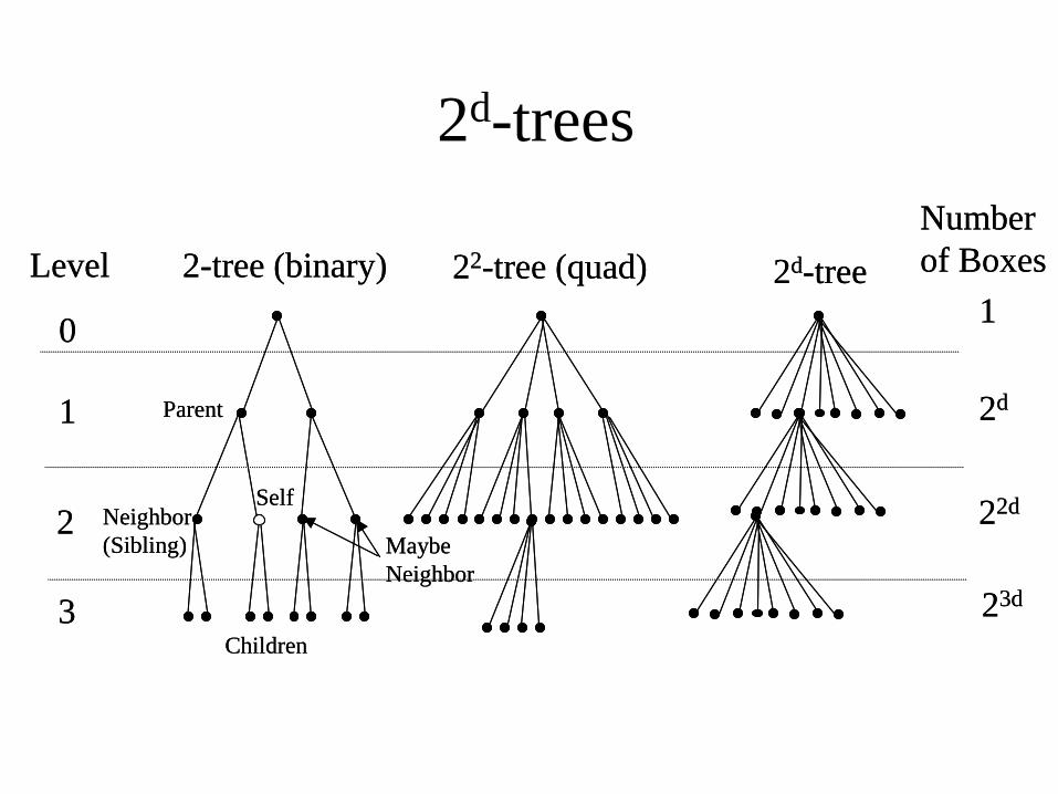
2d-trees
2-tree (binary) 22-tree (quad) 2d-tree
0
1
2
3
Level
Children
Parent
Neighbor(Sibling) Maybe
Neighbor
Self
Numberof Boxes
1
2d
22d
23d
2-tree (binary) 22-tree (quad) 2d-tree
0
1
2
3
Level
Children
Parent
Neighbor(Sibling) Maybe
Neighbor
Self
Numberof Boxes
1
2d
22d
23d

Hierarchical Numbering (Indexing) in 2d-trees. Numbering (Indexing) String.
0 01 2
1 31
3
3
3
31
1
1
0
20 0
02 2
2
1
11
1
1
111
11
11
1 1 1
0
0
0
00 0
0
0
0
0 00
0
0
0
2
0
2 2 2 2
222
2 2
222
2
2
2
3 3 3 3
3
3
3 33
3 3 3
33330 01 2
1 31
3
3
3
31
1
1
0
20 0
02 2
2
1
11
1
1
111
11
11
1 1 1
0
0
0
00 0
0
0
0
0 00
0
0
0
2
0
2 2 2 2
222
2 2
222
2
2
2
3 3 3 3
3
3
3 33
3 3 3
3333
Numbering in quad-tree
Numbering string
The large black box has the numbering string (2,3); The small black box has the numbering string (3,1,2);
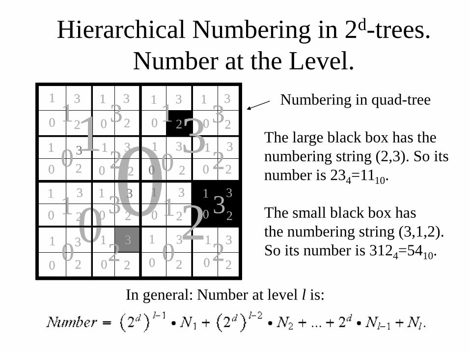
Hierarchical Numbering in 2d-trees. Number at the Level.
0 01 2
1 31
3
3
3
31
1
1
0
20 0
02 2
2
1
11
1
1
111
11
11
1 1 1
0
0
0
00 0
0
0
0
0 00
0
0
0
2
0
2 2 2 2
222
2 2
222
2
2
2
3 3 3 3
3
3
3 33
3 3 3
33330 01 2
1 31
3
3
3
31
1
1
0
20 0
02 2
2
1
11
1
1
111
11
11
1 1 1
0
0
0
00 0
0
0
0
0 00
0
0
0
2
0
2 2 2 2
222
2 2
222
2
2
2
3 3 3 3
3
3
3 33
3 3 3
3333
Numbering in quad-tree
The large black box has the numbering string (2,3). So its number is 234=1110. The small black box has the numbering string (3,1,2). So its number is 3124=5410.
In general: Number at level l is:

Hierarchical Numbering in 2d-trees. Universal Number.
0 01 2
1 31
3
3
3
31
1
1
0
20 0
02 2
2
1
11
1
1
111
11
11
1 1 1
0
0
0
00 0
0
0
0
0 00
0
0
0
2
0
2 2 2 2
222
2 2
222
2
2
2
3 3 3 3
3
3
3 33
3 3 3
33330 01 2
1 31
3
3
3
31
1
1
0
20 0
02 2
2
1
11
1
1
111
11
11
1 1 1
0
0
0
00 0
0
0
0
0 00
0
0
0
2
0
2 2 2 2
222
2 2
222
2
2
2
3 3 3 3
3
3
3 33
3 3 3
3333
Numbering in quad-tree
The large black box has the numbering string (2,3). So its number is 234=1110 at level 2 The small gray box has the numbering string (0,2,3). So its number is 234=1110 at level 3.
In general: Universal number is a pair:
This number at this level
Parent Index (Number)
0 01 2
1 31
3
3
3
31
1
1
0
20 0
02 2
2
1
11
1
1
111
11
11
1 1 1
0
0
0
00 0
0
0
0
0 00
0
0
0
2
0
2 2 2 2
222
2 2
222
2
2
2
3 3 3 3
3
3
3 33
3 3 3
33330 01 2
1 31
3
3
3
31
1
1
0
20 0
02 2
2
1
11
1
1
111
11
11
1 1 1
0
0
0
00 0
0
0
0
0 00
0
0
0
2
0
2 2 2 2
222
2 2
222
2
2
2
3 3 3 3
3
3
3 33
3 3 3
3333
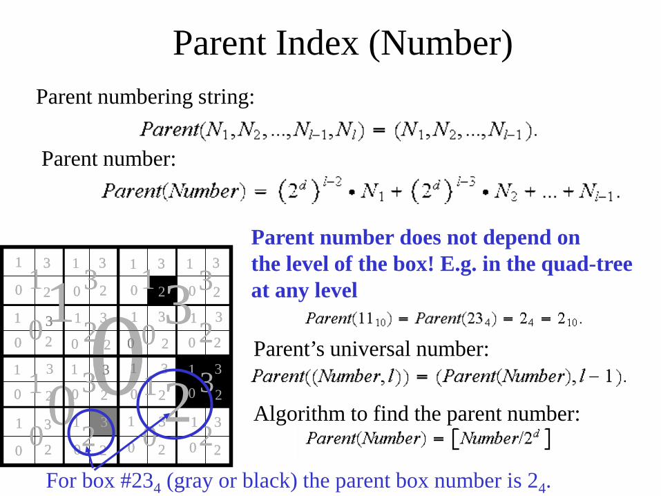
Parent numbering string:
Parent number:
Parent’s universal number:
Parent number does not depend on the level of the box! E.g. in the quad-tree at any level
Algorithm to find the parent number:
For box #234 (gray or black) the parent box number is 24.

Children Indices (Numbers) Children numbering strings:
Children numbers:
Children universal numbers:
Children numbers do not depend on the level of the box! E.g. in the quad-tree at any level:
Algorithm to find the children numbers:

A couple of examples:
Can it be even faster?
YES! USE BITSHIFT PROCEDURES!
(HINT: Multiplication and division by 2d
are equivalent to d-bit shift.)
Matlab Program for Parent Finding
p = bitshift(n,-d);
Spatial Ordering
These algorithms of Parent and Children finding are beautiful (O(1)), but how about neighbor finding? Also we need to find box center coordinates… The answer is SPATIAL ORDERING.
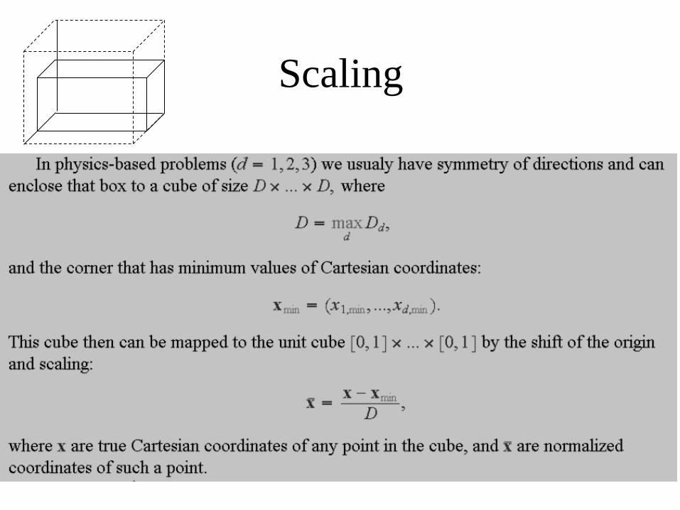
Scaling
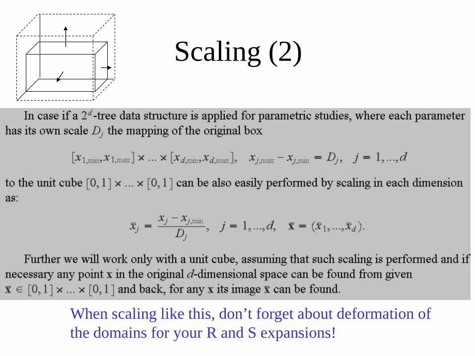
Scaling (2)
When scaling like this, don’t forget about deformation of the domains for your R and S expansions!
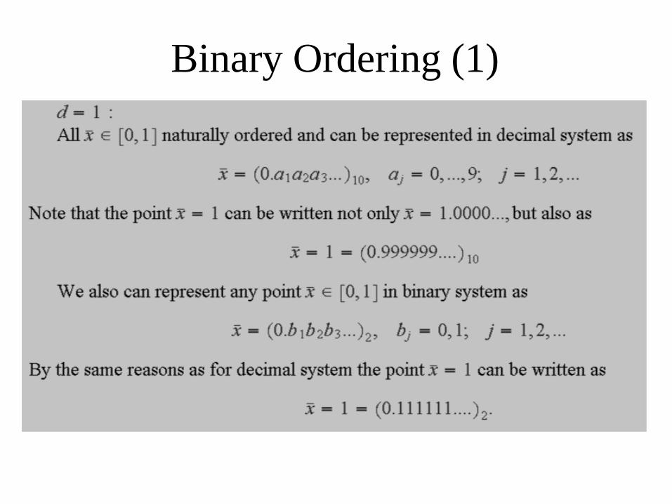
Binary Ordering (1)

Binary Ordering (2) Finding the number of the box
containing a given point
Level 1:
Level 2:
Level l: We use numbering strings !
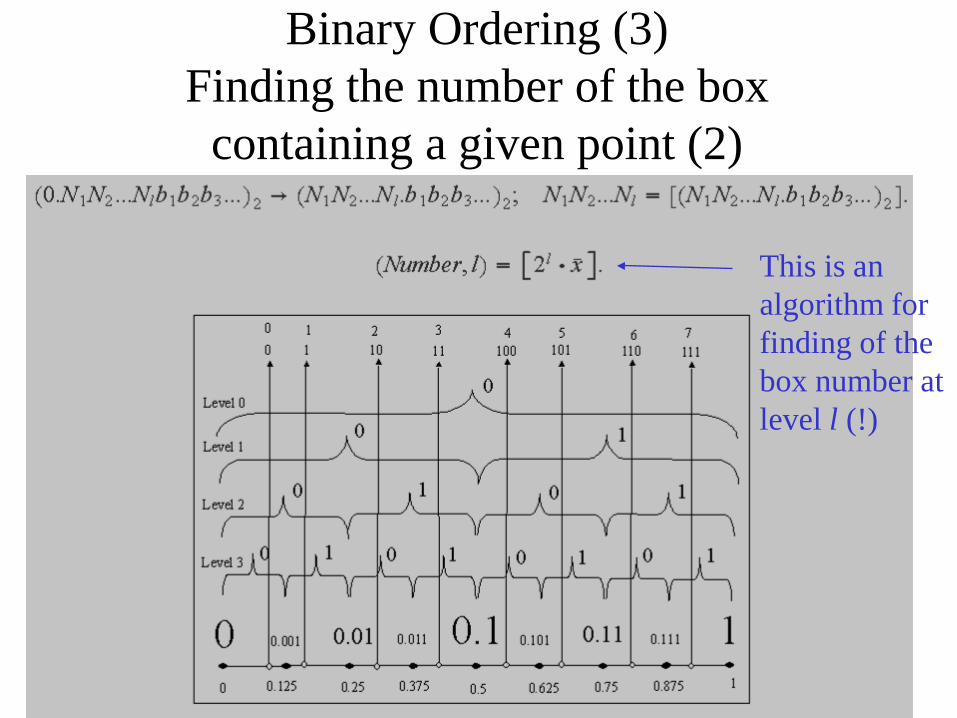
Binary Ordering (3) Finding the number of the box
containing a given point (2)
This is an algorithm for finding of the box number at level l (!)
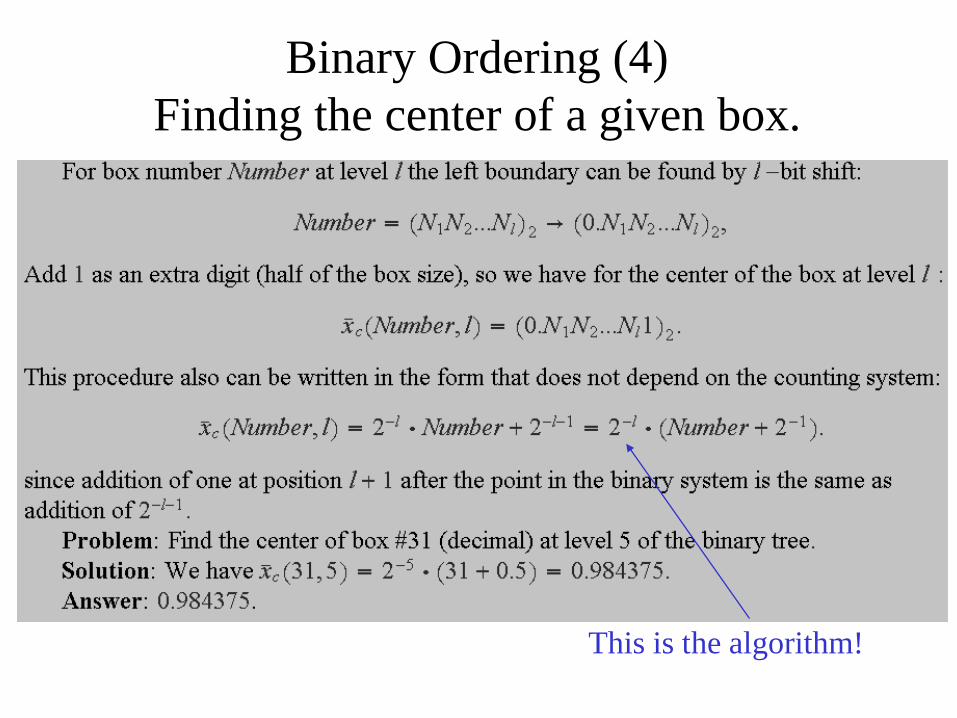
Binary Ordering (4) Finding the center of a given box.
This is the algorithm!
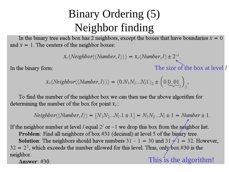
Binary Ordering (5) Neighbor finding
This is the algorithm!
The size of the box at level l
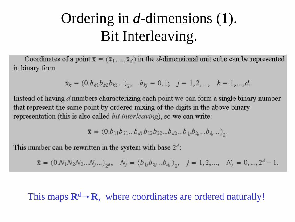
Ordering in d-dimensions (1). Bit Interleaving.
This maps Rd R, where coordinates are ordered naturally!
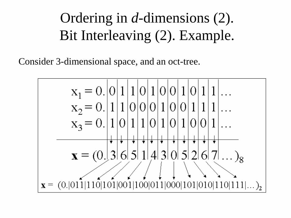
Ordering in d-dimensions (2). Bit Interleaving (2). Example.
Consider 3-dimensional space, and an oct-tree.
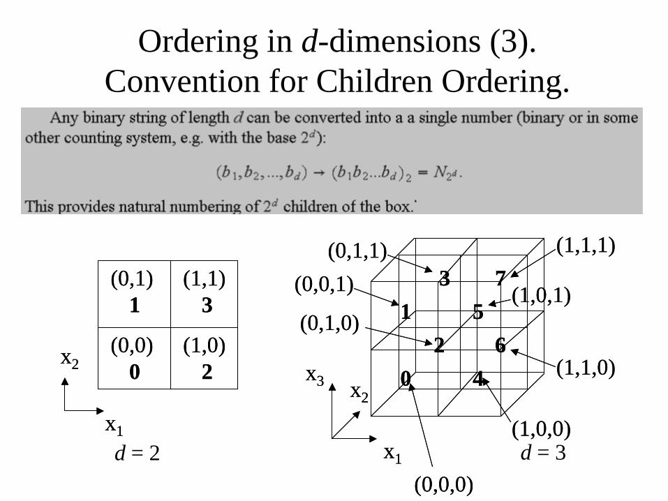
Ordering in d-dimensions (3). Convention for Children Ordering.
x1
x2(0,0)
0
(0,1)1
(1,0)2
(1,1)3
x1
x3 x2
(0,0,0)
(1,0,0)
0
12
3
4
56
7
(0,1,0)
(0,1,1)(0,0,1)
(1,1,0)
(1,1,1)
(1,0,1)
x1
x2(0,0)
0
(0,1)1
(1,0)2
(1,1)3
x1
x3 x2
(0,0,0)
(1,0,0)
0
12
3
4
56
7
(0,1,0)
(0,1,1)(0,0,1)
(1,1,0)
(1,1,1)
(1,0,1)
d = 2 d = 3
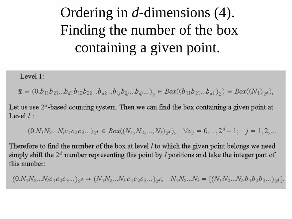
Ordering in d-dimensions (4). Finding the number of the box
containing a given point.
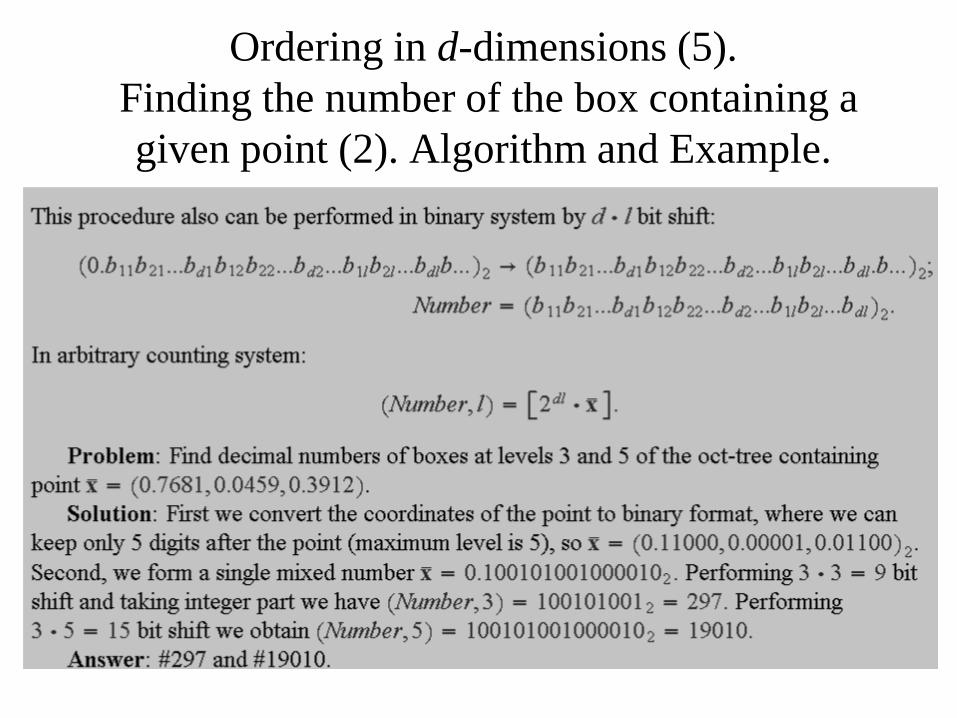
Ordering in d-dimensions (5). Finding the number of the box containing a
given point (2). Algorithm and Example.
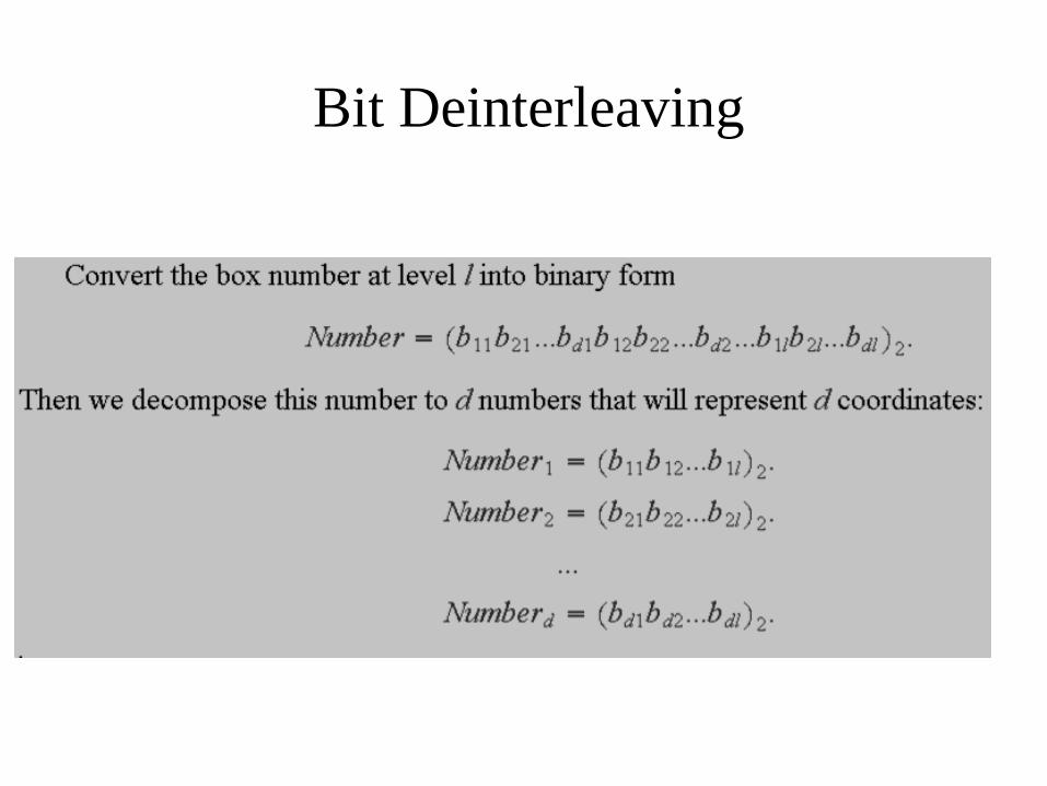
Bit Deinterleaving
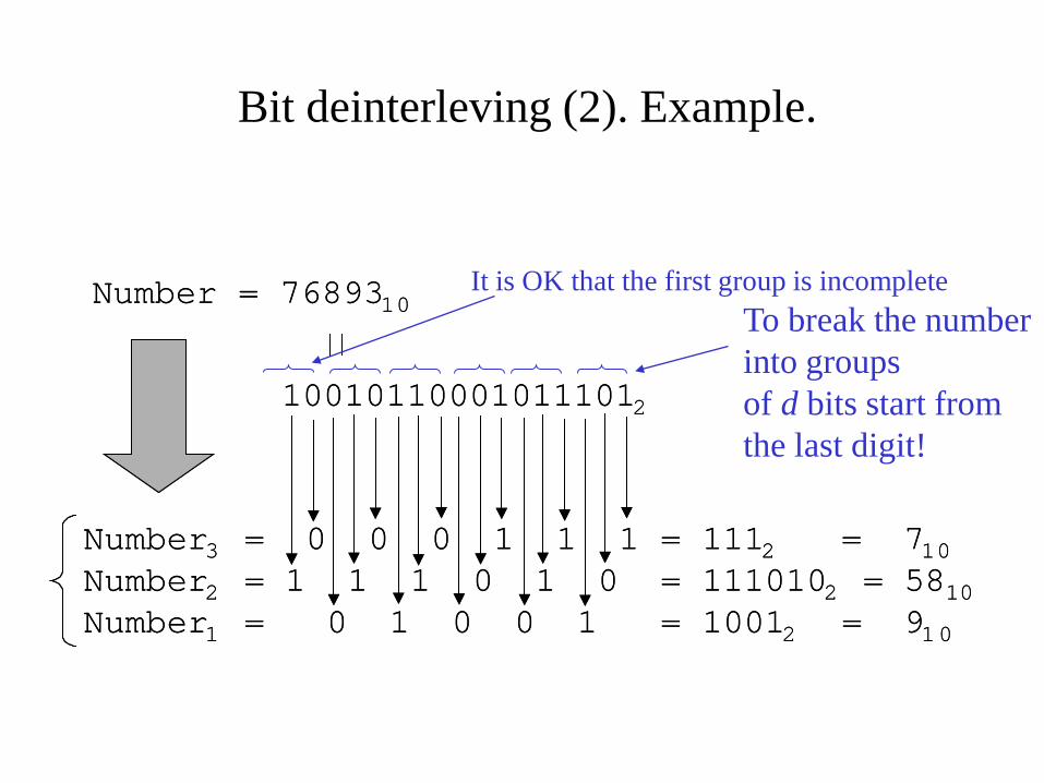
Bit deinterleving (2). Example.
100101100010111012
Number3 = 0 0 0 1 1 1 = 1112 = 710Number2 = 1 1 1 0 1 0 = 1110102 = 5810Number1 = 0 1 0 0 1 = 10012 = 910
Number = 7689310
100101100010111012
Number3 = 0 0 0 1 1 1 = 1112 = 710Number2 = 1 1 1 0 1 0 = 1110102 = 5810Number1 = 0 1 0 0 1 = 10012 = 910
Number = 7689310 To break the number into groups of d bits start from the last digit!
It is OK that the first group is incomplete
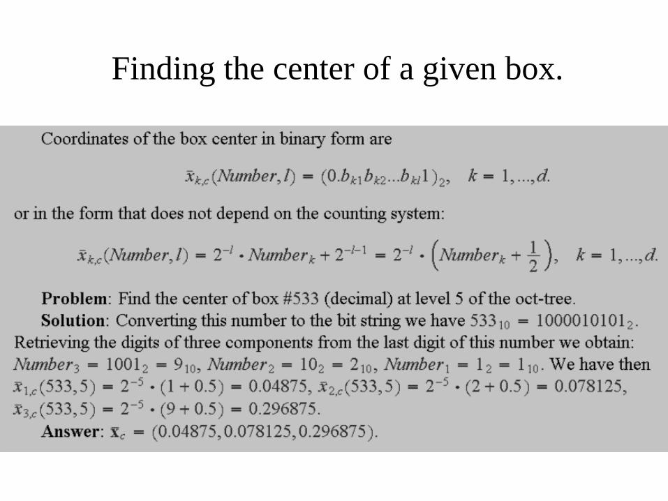
Finding the center of a given box.
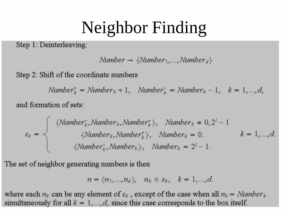
Neighbor Finding

Neighbor Finding (2). Example.
17
5
2921
1
45
574925
6153
3713
9 33 41
20
4
16
80 32
28
40
24
12 4436
56
52
48
2
60
6 14 38 46
423410
26 50
625430
18
22
58
23 31 55 63
19
7
27 5951
15 39 47
4335113
x1
x2 0 1 2 3 4 5 6 7Number1
0
1
2
3
4
5
6
7
Number2
17
5
2921
1
45
574925
6153
3713
9 33 41
20
4
16
80 32
28
40
24
12 4436
56
52
48
2
60
6 14 38 46
423410
26 50
625430
18
22
58
23 31 55 63
19
7
27 5951
15 39 47
4335113
x1
x2 0 1 2 3 4 5 6 7Number1
0
1
2
3
4
5
6
7
Number2
2610= 110102
(11,100)2 = (3,4)10
deinterleaving
generation of neighbors
(2,3) ,(2,4),(2,5),(3,3), (3,5),(4,3),(4,4),(4,5) = (10,11),(10,100),(10,101), (11,11),(11,101),(100,11), (100,100),(100,101) interleaving
1101,11000,11001,1111,11011,100101,110000,110001 = 13, 24, 25, 15, 27, 37, 48, 49
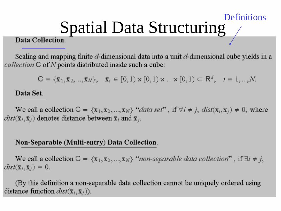
Spatial Data Structuring Definitions
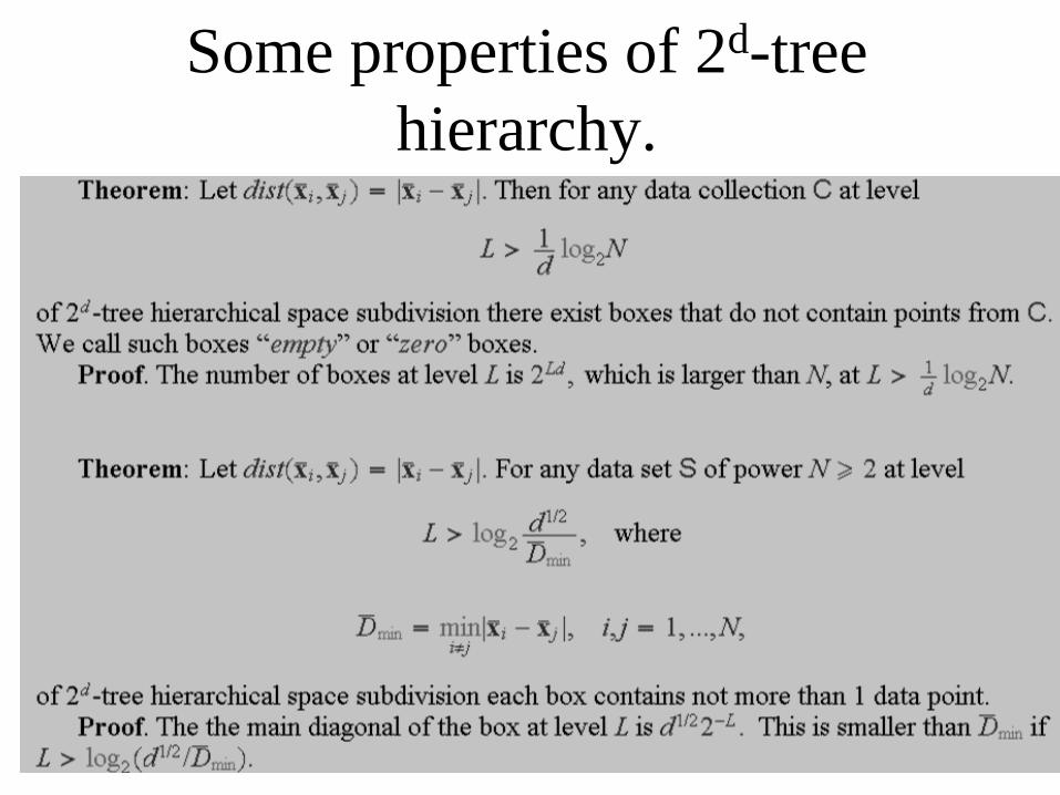
Some properties of 2d-tree hierarchy.
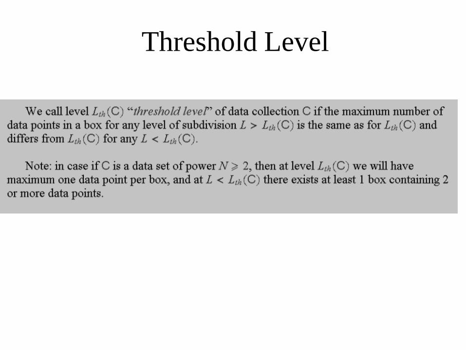
Threshold Level

Some Practical Issues Related to Spatial Ordering
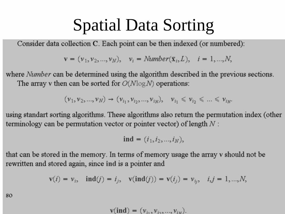
Spatial Data Sorting
Spatial Data Sorting (2)
• Before sorting represent your data with maximum number of bits available (or intended to use). This corresponds to maximum level Lavailable available (say [Lavailable =BitMax/d].
• In the hierarchical 2d-tree space subdivision the sorted list will remain sorted at any level L< Lavailable. So the data ordering is required only one time.
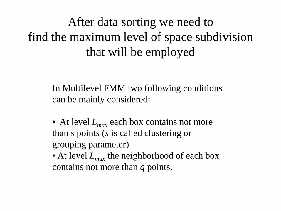
After data sorting we need to find the maximum level of space subdivision
that will be employed
In Multilevel FMM two following conditions can be mainly considered: • At level Lmax each box contains not more than s points (s is called clustering or grouping parameter) • At level Lmax the neighborhood of each box contains not more than q points.
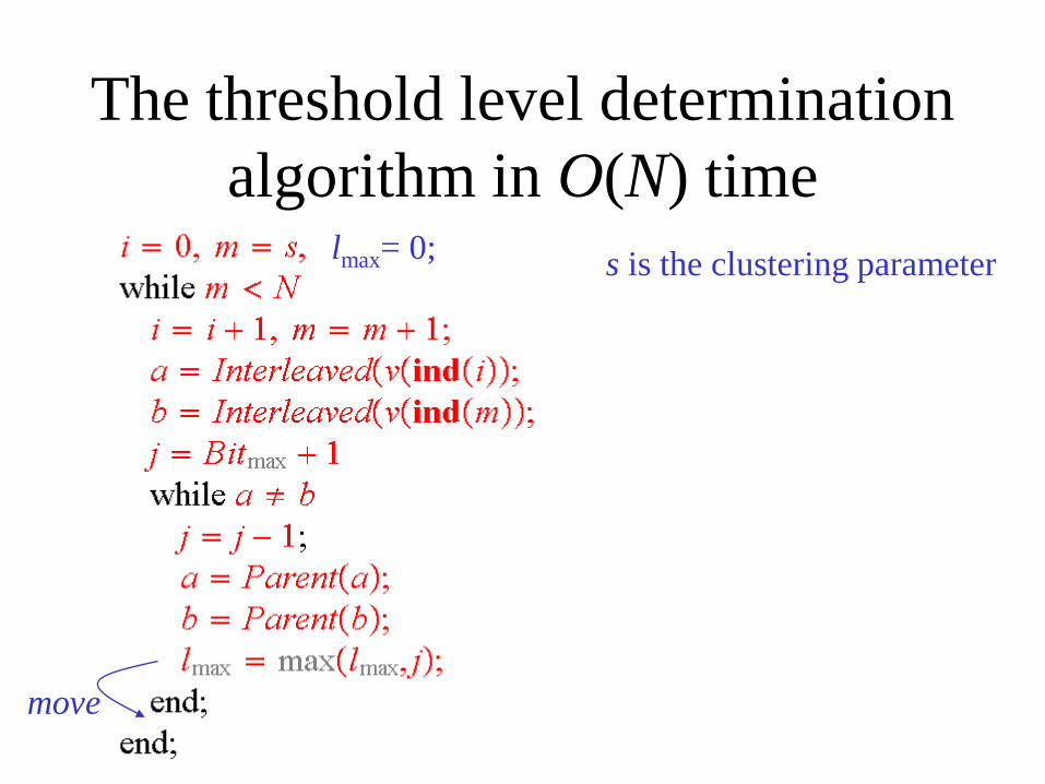
The threshold level determination algorithm in O(N) time
s is the clustering parameter lmax= 0;
move
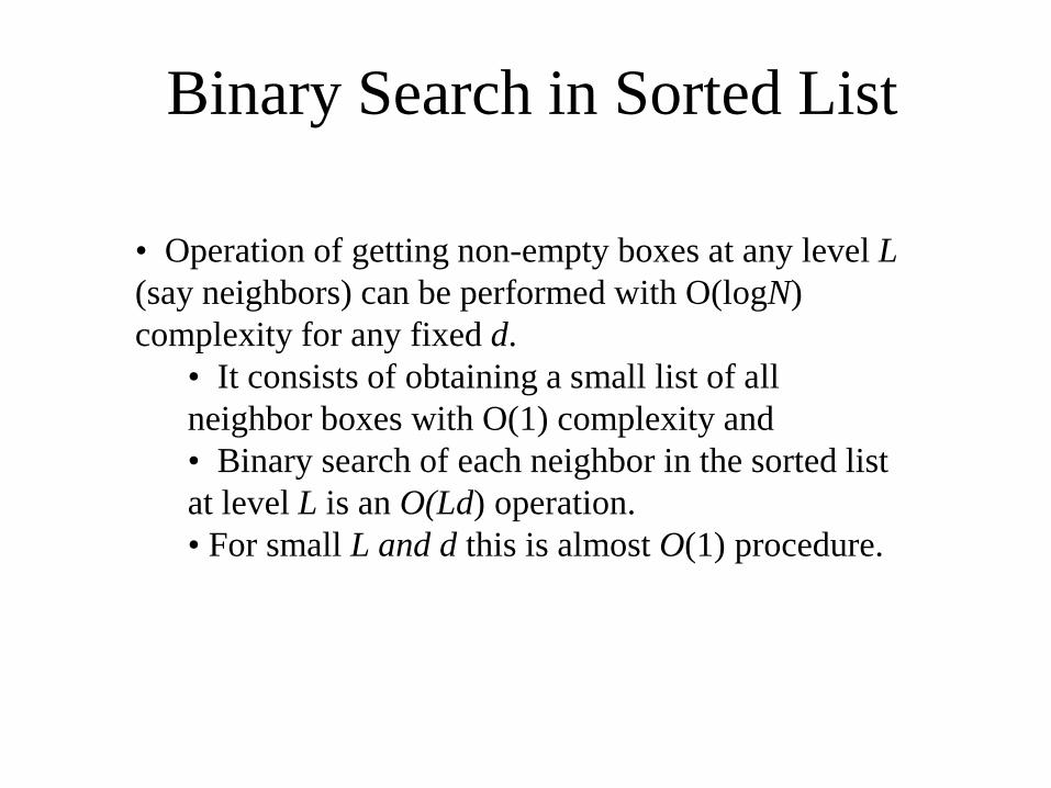
Binary Search in Sorted List
• Operation of getting non-empty boxes at any level L (say neighbors) can be performed with O(logN) complexity for any fixed d.
• It consists of obtaining a small list of all neighbor boxes with O(1) complexity and • Binary search of each neighbor in the sorted list at level L is an O(Ld) operation. • For small L and d this is almost O(1) procedure.
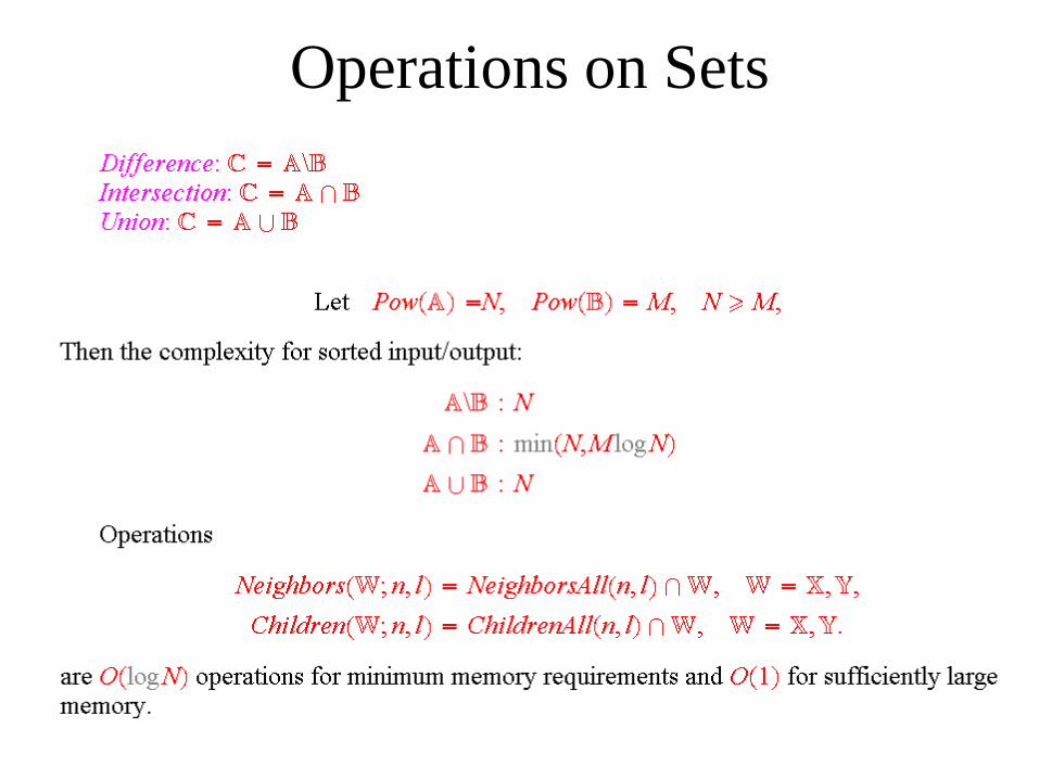
Operations on Sets

Practical recommendations for the FMM
• Even though you can write an O(logN) algorithm for getting all necessary information – don’t do that, if you have sufficient memory.
• Instead at the step of setting the data structure precompute and store all box indices (sources and receivers), Children (sources and receivers), E2 and E4 neighbor lists for all receivers (neighbor sources for receivers).
• If memory is sufficient, precompute and store all translation operators (S|S, S|R, R|R).
• Create a data structure, which allows you efficiently retrieve translation operator data.


