Date post: | 25-Dec-2015 |
Category: |
Documents |
Upload: | lester-hawkins |
View: | 214 times |
Download: | 0 times |
Nanocomputer
Systems EngineeringMichael P. Frank
University of FloridaCollege of Engineering
Departments of CISE and [email protected]
NanoEngineering World ForumInternational Engineering Consortium
Marlborough, MassachusettsJune 23-25, 2003
Laying the Key Methodological
Foundations for the Design of 21st-Century Computer Technology
Abstract• What is Nanocomputer Systems Engineering?
– Interdisciplinary engineering of computers w. nanoscale parts.– Recognizes tight interplay between physics and computing.
• Physical Computing Theory– Models of computing based on fundamental physics.– Powerful, accurate, and technology-independent.– Key capabilities include reversible and quantum computing.
• Technology Scaling and Systems Analysis– Compared cost-efficiency of reversible vs. irreversible technologies.– Reversible computing may win by factors of ≥1,000× by mid-century.– We outline how this projection was obtained.
• Conclusion: More attention should be paid to the design of reversible, ballistic device mechanisms.– Low leakage, high Q factor will both be critically important in bit-device
engineering for nanocomputers.
Organization of Talk
1. Moore’s Law vs. Fundamental Physics
2. Methodological Principles of NCSE
3. Physical Computing Theory
4. Reversible Computing
5. Cost-Efficiency Analysis of RC
6. Conclusions
Organization of Talk
1. Moore’s Law vs. Nanoscale Limits
2. Methodological Principles of NCSE
3. Physical Computing Theory
4. Reversible Computing
5. Cost-Efficiency Analysis of RC
6. Conclusions
Moore’s Law – Devices per IC
1
10
100
1,000
10,000
100,000
1,000,000
10,000,000
100,000,000
1,000,000,000
1950 1960 1970 1980 1990 2000 2010
Avg. increaseof 57%/year
4004
8086286
386486DX Pentium
P2P3
P4Itanium 2
Madison
Early Fairchild
ICs
Intel µpu’s
Super-Exponential Long-Term Trend
Across Multiple TechnologiesAcross Multiple Technologies
Source: Kurzweil, The Age of Spiritual Machines, pp. 22-25
Mechanical
ElectromechanicalRelays
Vacuum Tubes
DiscreteTransistors
IntegratedCircuits
Ops/second/$1,000
Source: Kurzweil ‘99
1900 2000
ITRS Feature Size Projections
0.1
1
10
100
1000
10000
100000
1000000
1955 1960 1965 1970 1975 1980 1985 1990 1995 2000 2005 2010 2015 2020 2025 2030 2035 2040 2045 2050
Year of First Product Shipment
Fe
atu
re S
ize
(n
an
om
ete
rs)
uP chan L
DRAM 1/2 p
min Tox
max Tox
Atom
We are here
Bacterium
Virus
Proteinmolecule
DNA moleculethickness
Eukaryoticcell
Human hairthickness
ITRS Feature Size Projections
0.1
1
10
100
1000
1995 2000 2005 2010 2015 2020 2025 2030 2035 2040 2045 2050
Year of First Product Shipment
Fe
atu
re S
ize
(n
an
om
ete
rs)
uP chan L
DRAM 1/2 p
min Tox
max Tox
Atom
We are here
Virus
Proteinmolecule
DNA moleculethickness
Bacterium
A Precise Definition of Nanoscale
10−6 m = 1 µm
10−9 m = 1 nm
10−12 m = 1 pm
10−7.5 m ≈ 31.6 nm
10−10.5 m ≈ 31.6 pm
Nanoscale:Characteristic length scale ofNanocomputers
Microscale: Characteristic length scale ofMicrocomputers
10−4.5 m ≈ 31.6 µm
Picoscale:Characteristic length scale ofPicocomputers (if possible)
Nearnano-scaleFarnano-scale
~Atom size
Trend of minimum transistor switching energy
1
10
100
1000
10000
100000
1000000
1995 2005 2015 2025 2035
Year of First Product Shipment
Min
tra
ns
isto
r s
wit
ch
ing
en
erg
y, kTs
High
Low
trend
Organization of Talk
1. Moore’s Law vs. Fundamental Physics
2. Methodological Principles of NCSE
3. Physical Computing Theory
4. Reversible Computing
5. Cost-Efficiency Analysis of RC
6. Conclusions
Key Principles of NCSE
• Design for Generalized Cost-Efficiency
• Physics-Based Modeling
• Technology-Independent Models
• Multi-Domain Modeling
• Hierarchical Modeling
• Global System Design Optimization
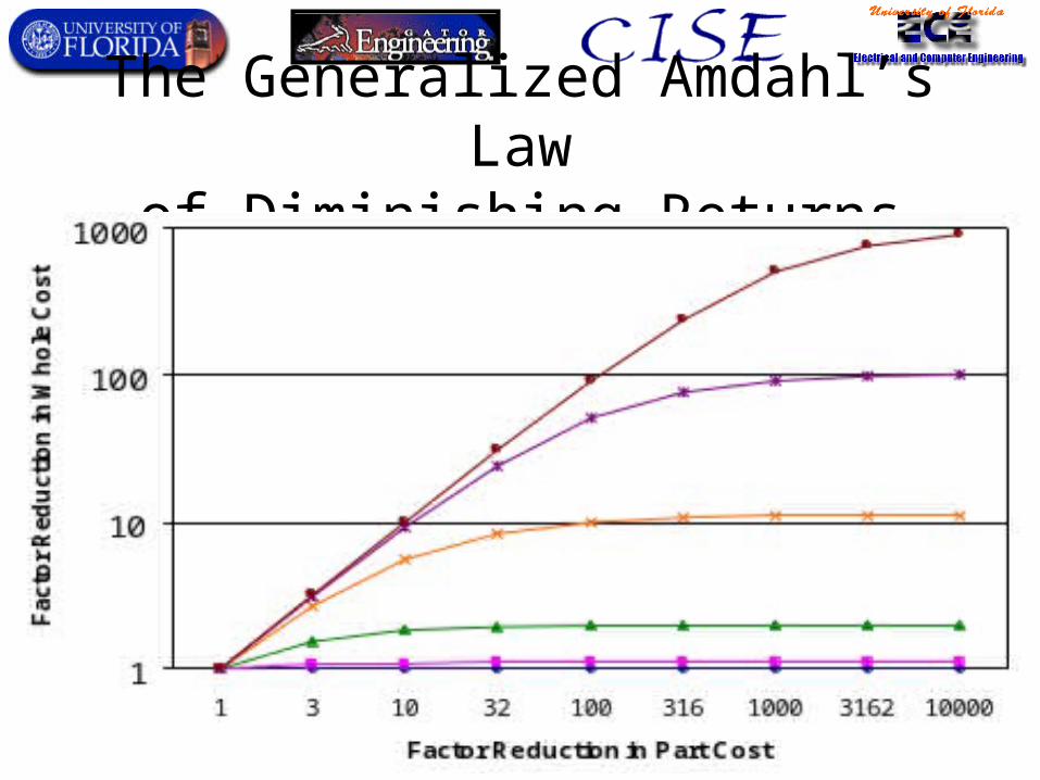
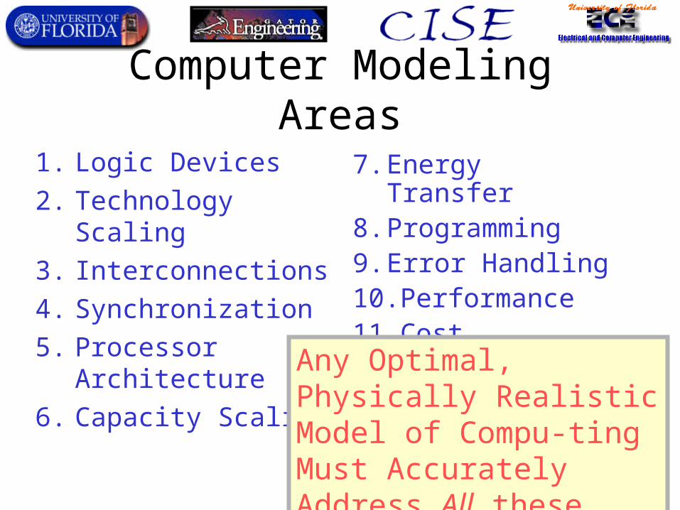
• Claim: All practical engineering design-optimization can arguably be ultimately reduced to maximization of a generalized, system-level cost-efficiency characteristic.– Given an appropriate model of cost “$”.
• Definition of the Cost-Efficiency %$ of a process: %$ ≝ $min/$actual
• Maximize %$ by minimizing $actual
– Note: This is valid even when $min is unknown
Cost-Efficiency:The Key Figure of Merit
Important Cost Categories in Computing
• Hardware-Proportional Costs:– Initial Manufacturing Cost
• Time-Proportional Costs:– Inconvenience to User Waiting for Result
• (HardwareTime)-Proportional Costs:– Amortized Manufacturing Cost– Maintenance & Operation Costs– Opportunity Costs
• Energy-Proportional Costs:– Adiabatic Losses– Non-adiabatic Losses From Bit Erasure– Note: These may both vary
independently of (HWTime)!
Focus of mosttraditionaltheory aboutcomputational“complexity.”
These costsmust be included also in practicaltheoreticalmodels ofnanocomputing!
Computer Modeling Areas
1. Logic Devices
2. Technology Scaling
3. Interconnections
4. Synchronization
5. Processor Architecture
6. Capacity Scaling
7. Energy Transfer8. Programming9. Error Handling10.Performance11.Cost
Any Optimal, Physically Realistic Model of Compu-ting Must Accurately Address All these Areas!
Hierarchical System Design• Abstract from sub-component
designs to values of keysummary characteristics.
• Separates super-systemdesign from sub-system design.
• Facilitates globaloptimization ofsystem across alllevels of design.
Enclosing System S:design variables
vS1, vS2, …
Subsystem T:design
variablesvT1, vT2, …
Subsystem U:design
variablesvT1, vT2, …
Summarycharacteristics
cT1, cT2, …
SummarycharacteristicscU1, cU2, …
Summarycharacteristics of lower-level
subsystems
Summary characteristicscS1, cS2, …
Three-Pass System Optimization
Top-level System S:Design variables VS
Mid-level Subsystem T:Design variables VT
Low-level Component U, Design variables VU
Summary characteristics CS
Summary characteristics CT
Summary characteristics CU CU(VU) = …
CT(VT, CU) = …
CS(VS, CT) = … opt VS(CT)
= …
opt VT(CU) = …
opt VU = … VU := opt
VU
VT := opt VT(CU(VU))
VS := opt VS(CT(VT))
Pass #1 Pass #2 Pass #3
• A general methodology for the interdisciplinary optimization of the design of complex systems.
1) Express system performance characteristics as functions ofcomponent design variables.
2) Composeoptimizationprocedures.
3) Select optimized values of design parameters.
Organization of Talk
1. Moore’s Law vs. Fundamental Physics
2. Methodological Principles of NCSE
3. Physical Computing Theory
4. Reversible Computing
5. Cost-Efficiency Analysis of RC
6. Conclusions
Fundamental Physical Limits of Computing
Speed-of-LightLimit
Thoroughly Confirmed
Physical Theories
UncertaintyPrinciple
Definitionof Energy
Reversibility
2nd Law ofThermodynamics
Adiabatic Theorem
Gravity
Theory ofRelativity
QuantumTheory
ImpliedUniversal Facts
Affected Quantities in Information Processing
Communications Latency
Information Capacity
Information Bandwidth
Memory Access Times
Processing Rate
Energy Loss per Operation
Landauer’s 1961 principle from basic quantum theory
…Ndistinct
states
Ndistinct
states
……
2Ndistinctstates
Unitary(1-1)
evolution
Before bit erasure: After bit erasure:
Increase in entropy: S = log 2 = k ln 2. Energy lost to heat: ST = kT ln 2
0s0
0sN−1
…
1s′0
1s′N−1
…
…
0s″0
0s″N−1
0s″N
0s″2N−1
…
CORP: Computing with Optimal Realistic Physics
• A comprehensive model based on the RQ3M: – The Reversible/Quantum 3-Dimensional Mesh– A proposed “ultimate” (UMS) model of computing.– Universally Maximally Scalable (UMS):
• Means, as efficient as any physically possible computing machine at any given problem, within at worst a constant asymptotic factor.
– “Tight Church’s Thesis:” My proposed conjecture, that the RQ3D is, in fact, a UMS model.
CORP Device Model• Physical degrees of freedom (sub-state-spaces)
broken down into coding and non-coding parts.– These are then further subdivided as shown below.
• Components are characterized by geometry, delay, & operating & interaction temperatures within & between devices and their subsystems and subcomponents.
Device
CodingSubsystem
Non-codingSubsystem
LogicalSubsystem
RedundancySubsystem
StructuralSubsystem
ThermalSubsystem
CORP Technology Scaling Model• For simplicity, assume ordinary Moore’s Law
type scaling until nanoscale limits are reached.
• Some important limiting considerations:– Entropy densities in (atomic) materials at normal
pressures max out around 1 bit per cubic Ångstrom.• Achieving significantly greater densities appears to require
infeasibly high pressures.
– Room temperature (300K) corresponds to a maximum frequency of quantum bit-operations of 12.5 THz.
• Significantly higher temperatures cause melting of all atomic structures, except at extremely high pressures.
CORP Capacity Scaling Model
• Multiprocessing model
• Mesh-type (locally connected) interconnect structure
• Thermal pathways explicitly represented!
• Scaling in 3D up to thermal limits
• Device frequencies can be scaled down as number of devices increases, for maximum energy efficiency and cost-efficiency
Other Aspects of CORP Modeling• Interconnect & Timing Models
– Interconnects and oscillators can be treated as just special cases of devices.
– Generalized mesh-style interconnect network.
• Architectural Model (Logic gates up to Processors)– Architectural design tools & methodologies should not
preclude efficient reversible & quantum hardware designs!
• Programming Model– Should support standard programming paradigms.
– But, should also permit expressing efficient reversible & quantum algorithms, in cases where these are beneficial.
Organization of Talk
1. Moore’s Law vs. Fundamental Physics
2. Methodological Principles of NCSE
3. Physical Computing Theory
4. Reversible Computing
5. Cost-Efficiency Analysis of RC
6. Conclusions
Terminology / RequirementsProperty of Computing Mechanism Approximate Meaning
Required for Quantum Computing?
Required for Reversible
Computing?
(Treated As)Unitary
System’s full invertible quantum evolution, w. all phase information, is modeled & tracked
Yes, device & system evolution must be modeled as ~unitary, within threshold
No, only reversible evolution of classical state variables need be tracked
Coherent Pure quantum statesdon’t decohere (for us) into statistical mixtures
Yes, must maintain full global coherence, locally within threshold
No, only maintain stability of local pointer states+transitions
Adiabatic No entropy flow in/out of computational subsystem
Yes, must be above a certain threshold
Yes, as high as possible
Isentropic / Thermodynamically
Reversible
No new entropy generated by mechanism
Yes, must be above a certain threshold
Yes, as high as possible
Time-Independent Hamiltonian,
Self-Controlled
Closed system, evolves autonomously w/o external control
No, transitions can be externally timed & controlled
Yes, if we care about energy dissipation in the driving system
Ballistic System evolves w. net forward momentum
No, transitions can be externally driven
Yes, if we care about performance
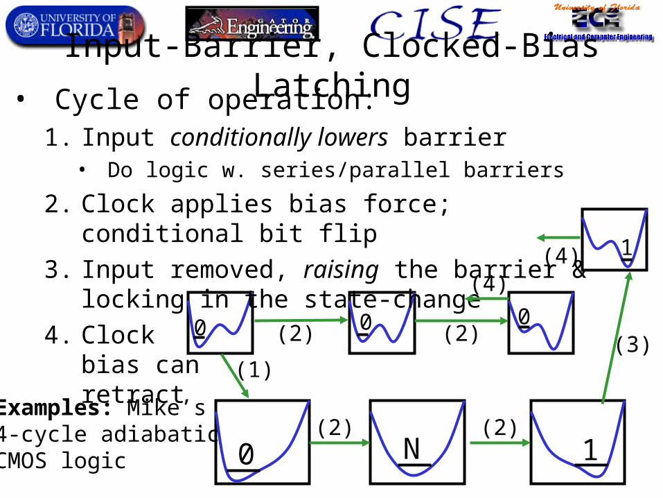
Some Claims Against Reversible Computing Eventual Resolution of Claim
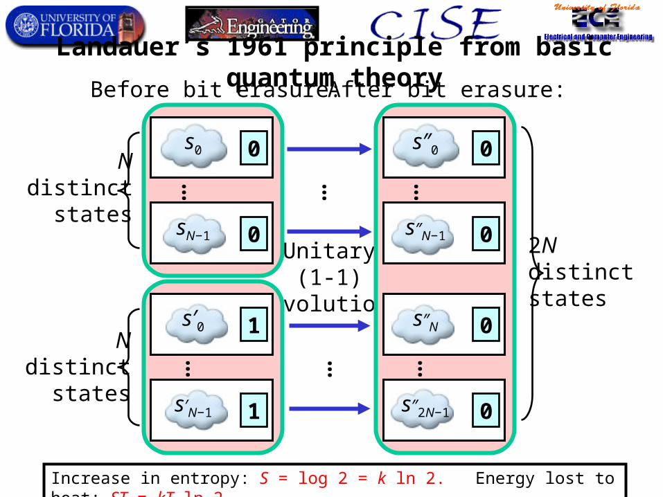
John von Neumann, 1949 – Offhandedly remarks during a lecture that computing requires kT ln 2 dissipation per “elementary act of decision” (bit-operation).
No proof provided. Twelve years later, Rolf Landauer of IBM tries valiantly to prove it, but succeeds only for logically irreversible operations.
Rolf Landauer, 1961 – Proposes that the logically irreversible operations which necessarily cause dissipation are unavoidable.
Landauer’s argument for unavoidability of logically irreversible operations was conclusively refuted by Bennett’s 1973 paper.
Bennett’s 1973 construction is criticized for using too much memory. Bennett devises a more space-efficient version of the algorithm in 1989.
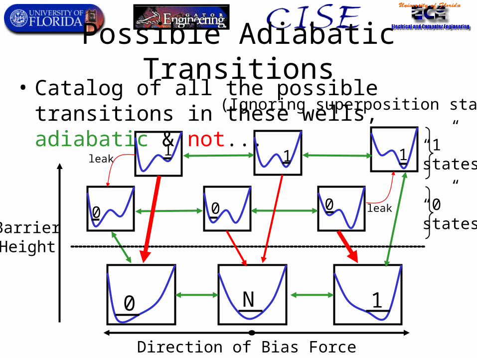
Bennett’s models criticized by various parties for depending on random Brownian motion, and not making steady forward progress.
Fredkin and Toffoli at MIT, 1980, provide ballistic “billiard ball” model of reversible computing that makes steady progress.
Various parties note that Fredkin’s original classical-mechanical billiard-ball model is chaotically unstable.
Zurek, 1984, shows that quantum models can avoid the chaotic instabilities. (Though there are workable classical ways to fix the problem also.)
Various parties propose that classical reversible logic principles won’t work at the nanoscale, for unspecified or vaguely-stated reasons.
Drexler, 1980’s, designs various mechanical nanoscale reversible logics and carefully analyzes their energy dissipation.
Carver Mead, CalTech, 1980 – Attempts to show that the kT bound is unavoidable in electronic devices, via a collection of counter-examples.
No general proof provided. Later he asked Feynman about the issue; in 1985 Feynman provided a quantum-mechanical model of reversible computing.
Various parties point out that Feynman’s model only supports serial computation. Margolus at MIT, 1990, demonstrates a parallel quantum model of reversible computing—but only with 1 dimension of parallelism.
People question whether the various theoretical models can be validated with a working electronic implementation.
Seitz and colleagues at CalTech, 1985, demonstrate working energy recovery circuits using adiabatic switching principles.
Seitz, 1985—Has some working circuits, unsure if arbitrary logic is possible. Koller & Athas, Hall, and Merkle (1992) separately devise general reversible combinational logics.
Koller & Athas, 1992 – Conjecture reversible sequential feedback logic impossible. Younis & Knight @MIT do reversible sequential, pipelineable circuits in 1993-94.
Some computer architects wonder whether the constraint of reversible logic leads to unreasonable design convolutions.
Vieri, Frank and coworkers at MIT, 1995-99, refute these qualms by demonstrating straightforward designs for fully-reversible, scalable gate arrays, microprocessors, and instruction sets.
Some computer science theorists suggest that the algorithmic overheads of reversible computing might outweigh their practical benefits.
Frank, 1997-2003, publishes a variety of rigorous theoretical analysis refuting these claims for the most general classes of applications.
Various parties point out that high-quality power supplies for adiabatic circuits seem difficult to build electronically.
Frank, 2000, suggests microscale/nanoscale electro mechanical resonators for high-quality energy recovery with desired waveform shape and frequency.
Frank, 2002—Briefly wonders if synchronization of parallel reversible computation in 3 dimensions (not covered by Margolus) might not be possible.
Later that year, Frank devises a simple mechanical model showing that parallel reversible systems can indeed be synchronized locally in 3 dimensions.
Bistable Potential-Energy Wells• Consider any system having an adjustable, bistable potential
energy surface (PES) in its configuration space.
• The two stable states form a natural bit.– One state represents 0, the other 1.
• Consider now the P.E. well havingtwo adjustable parameters:– (1) Height of the potential energy barrier
relative to the well bottom– (2) Relative height of the left and right
states in the well (bias)
0 1
(Landauer ’61)
Possible Parameter Settings• We will distinguish six qualitatively
different settings of the well parameters, as follows…
Direction of Bias Force
BarrierHeight
One Mechanical Implementation
spring spring
Rightwardbias
Leftwardbias
Barrier up
Barrier down
Barrierwedge
Stateknob
Possible Adiabatic Transitions• Catalog of all the possible transitions in
these wells, adiabatic & not...
Direction of Bias Force
BarrierHeight
0 0 0
111
10 N
(Ignoring superposition states.)
leak
leak
“1”states
“0”states
Ordinary Irreversible Logics• Principle of operation: Lower a barrier, or not,
based on input. Series/parallel combinations of barriers do logic. Major dissipation in at least one of
the possible transitions.0
1
0
Example: Ordinary CMOS logics
Input changes,barrier
lowered
Outputirreversiblychanged to 0
• Amplifies input signals.
Ordinary Irreversible Memory• Lower a barrier, dissipating stored information.
Apply an input bias. Raise the barrier to latch the new informationinto place. Remove inputbias.
0 0
11
10 NExample:DRAM
Dissipationhere can be
made as low as kT ln 2
Input“0”
Input“1”
Barrier up
Barrierup
Retractinput
Retractinput
Input-Bias Clocked-Barrier Logic• Cycle of operation:
– (1) Data input applies bias• Add forces to do logic
– (2) Clock signal raises barrier– (3) Data input bias removed
0 0
11
10 N
Can amplify/restore input signalin the barrier-raising step.
Can reset latch reversibly (4) given copy ofcontents.
Examples: AdiabaticQDCA, SCRL latch, Rod logic latch, PQ logic,Buckled logic
(1) (1)
(2)
(2)(3)
(3)
(4)(4)
(4) (4)
(4)
(4)
Input-Barrier, Clocked-Bias Retractile
• Cycle of operation:– Inputs raise or lower barriers
• Do logic w. series/parallel barriers
– Clock applies bias force which changes state, or not
0 0 0
10 N
• Barrier signal amplified.• Must reset output prior to input.• Combinational logic only!
(1) Input barrier height
(2) Clocked force applied
Examples:Hall’s logic,SCRL gates,Rod logic interlocks
Input-Barrier, Clocked-Bias Latching
0 0 0
1
10 N
• Cycle of operation:1. Input conditionally lowers barrier
• Do logic w. series/parallel barriers
2. Clock applies bias force; conditional bit flip
3. Input removed, raising the barrier &locking in the state-change
4. Clockbias canretract
Examples: Mike’s4-cycle adiabaticCMOS logic
(1)
(2) (2)
(2) (2)
(3)
(4)(4)
Sleeve
(a)
(b)
(c)
(d)
(e)
(f)
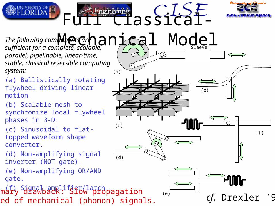
Full Classical-Mechanical ModelThe following components are sufficient for a complete, scalable, parallel, pipelinable, linear-time, stable, classical reversible computing system:
(a) Ballistically rotating flywheel driving linear motion.
(b) Scalable mesh to synchronize local flywheel phases in 3-D.
(c) Sinusoidal to flat-topped waveform shape converter.
(d) Non-amplifying signal inverter (NOT gate).
(e) Non-amplifying OR/AND gate.
(f) Signal amplifier/latch.
Primary drawback: Slow propagationspeed of mechanical (phonon) signals. cf. Drexler ‘92
• Energy storedmechanically.
• Variable couplingstrength → customwave shape.
• Can reduce lossesthrough balancing,filtering.
A MEMS Supply Concept
MEMS/NEMS Resonators• State of the art technologies demonstrated in lab:
– Frequencies up into the microwave (>1 GHz) regime– Q’s >10,000 in vacuum, several thousand even in air!
• Are rapidly becoming the technology of choicefor commercial RF filters, etc., in embeddedcommunicationsSoCs (Systems-on-a-Chip), e.g. for cellphones.
2LAL: 2-level Adiabatic Logic
• Use simplified T-gate symbol:
• Basic buffer element:– cross-coupled T-gates
• Only 4 timing signals,4 ticks per cycle: i rises during tick i
i falls during tick i+2 mod 4
P
P
P
:
in
out
1
0
0 1 2 3Tick #
0
1
2
3
(Implementable using ordinary CMOS transistors)
2LAL Cycle of Operation
in
in1
in=0
01
01
10
11
out1
out=0
00
00
in011
out0
Tick #0 Tick #1 Tick #2 Tick #3
2LAL Shift Register Structure• 1-tick delay per logic stage:
• Logic pulse timing & propagation:
in1
0
2
1
3
2
out
0
3
in
in
0 1 2 3 ... 0 1 2 3 ...
More complex logic functions• Non-inverting Boolean functions:
• For inverting functions, must use quad-rail logic encoding:– To invert, just
swap the rails!• Zero-transistor
“inverters.”
A
B
A
AB
A B
AB
A0
A0
A1
A1
A = 0 A = 1
Reversible / Adiabatic Chips Designed @ MIT, 1996-1999
By the author and other then-students in the MIT Reversible Computing group,under AI/LCS lab members Tom Knight and Norm Margolus.
Organization of Talk
1. Moore’s Law vs. Fundamental Physics
2. Methodological Principles of NCSE
3. Physical Computing Theory
4. Reversible Computing
5. Cost-Efficiency Analysis of RC
6. Conclusions
A Showcase Application of Our NCSE Methodology
• An important research question to be answered:– As nanocomputing technology advances,
will reversible computing ever become very cost-effective, and if so, when?
• We applied our methodology as follows:– Made Realistic Model (Obeying Constraints)– Optimized Cost-Efficiency in the Model– Swept Model Parameters over Future Years
Important Factors Included in Our Model
• Entropic cost of irreversibility
• Algorithmic overheads of reversible logic
• Adiabatic speed vs. energy-usage tradeoff
• Optimized degree of reversibility
• Limited quality factors of real devices
• Communications latencies in parallel algorithms
• Realistic heat flux constraints
Technology-Independent Model of Nanoscale Logic Devices
Id – Bits of internal logical state information per nano-device
Siop – Entropy generated per irreversible nano-device operation
tic – Time per device cycle (irreversible case)Sd,t – Entropy generated per device per unit time
(standby rate, from leakage/decay)Srop,f – Entropy generated per reversible op per unit frequencyd – Length (pitch) between neighboring nanodevicesSA,t – Entropy flux per unit area per unit time
Technological Trend Assumptions
1E-17
1E-16
1E-15
1E-14
1E-13
1E-12
1E-11
1E-10
1E-09
1E-08
1E-07
1E-06
0.00001
0.0001
0.001
0.01
0.1
1
10
100
1000
10000
100000
2000 2010 2020 2030 2040 2050 2060
Sia
tci
ld
Cd
Entropy generatedper irreversible bittransition, nats
Minimum time perirreversible bit-devicetransition, secs.
Minimum pitch (separation between centers of adjacent bit-devices), meters.
Minimum cost perbit-device, US$.
Absolute Absolute thermodynamicthermodynamiclower limit!lower limit!
Nanometer pitch limitNanometer pitch limit
Example Example quantum limitquantum limit
Fixed Technology Assumptions
• Total cost of manufacture: US$1,000.00– User will pay this for a high-performance desktop CPU.
• Expected lifetime of hardware: 3 years– After which machine is obsolete and mostly depreciated.
• Total power limit: 100 Watts– Much greater than this and it would burn up your lap!
• Power flux limit: 100 Watts per square centimeter– Approximate limit of air-cooling capabilities
• Standby entropy generation rate: 1,000 nat/s/device– Arbitrarily chosen, but achievable in today’s technology
Cost-Efficiency Benefits
1.00E+22
1.00E+23
1.00E+24
1.00E+25
1.00E+26
1.00E+27
1.00E+28
1.00E+29
1.00E+30
1.00E+31
1.00E+32
1.00E+33
2000 2010 2020 2030 2040 2050 2060
Bit
-ope
rati
ons
per
US
dol
lar
Bit
-ope
rati
ons
per
US
dol
lar
Conventional irreversib
le computing
Worst-cas
e revers
ible computin
g
Best-ca
se rev
ersible
computin
g
Scenario: $1,000/3-years, 100-Watt conventional computer, vs. reversible computers w. same capacity.
All curves would →0 if leakage
not reduced.
~1,000×
~100,000×
Scaling withdevice’s quantum“quality” factor q.
• The optimal redundancyfactor scales as: 1.1248(ln q)
• The minimumentropy gener-ation scales as: q −0.9039
Lower Limit to Entropy Generation Per Bit-Operation
Conclusions• We are developing an integrated and principled
methodological foundation for analysis in the new field of NanoComputer Systems Engineering (NCSE).– Techniques like our Physical Computing Theory are needed in
order to properly address important and difficult questions.• E.g., the realistic cost-efficiency of reversible computing.
• Results from our analytical models to date indicate that Reversible Computing offers extreme potential cost-efficiency advantages for future nanocomputing.– Even when taking its overheads into account!
• Thus, nanocomputing device engineers must focus harder on the requirements for efficient reversible operation:– E.g., Low per-device leakage rates, high resonant Q factors.