Nanofluid Flow Past a Stretching Plate Authors: Gabriella Bognár, Mohamad Klazly, Krisztián Hriczó Date Submitted: 2020-11-09 Keywords: Nusselt number, skin friction, similarity method, Computational Fluid Dynamics, nanofluid, moving surface, Sakiadis flow Abstract: Viscous nanofluid flow due to a sheet moving with constant speed in an otherwise quiescent medium is studied for three types of nanofluids, such as alumina (Al2O3), titania (TiO2), and magnetite (Fe3O4), in a base fluid of water. The heat and mass transfer characteristics are investigated theoretically using the boundary layer theory and numerically with computational fluid dynamics (CFD) simulation. The velocity, temperature, skin friction coefficient, and local Nusselt number are determined. The obtained results are in good agreement with known results from the literature. It is found that the obtained results for skin friction and for the Nusselt number are slightly greater than those obtained via boundary layer theory. Record Type: Published Article Submitted To: LAPSE (Living Archive for Process Systems Engineering) Citation (overall record, always the latest version): LAPSE:2020.1097 Citation (this specific file, latest version): LAPSE:2020.1097-1 Citation (this specific file, this version): LAPSE:2020.1097-1v1 DOI of Published Version: https://doi.org/10.3390/pr8070827 License: Creative Commons Attribution 4.0 International (CC BY 4.0) Powered by TCPDF (www.tcpdf.org)
Viscous nanofluid flow due to a sheet moving with constant speed in an otherwise quiescent medium is studied for three types ofnanofluids, such as alumina (Al2O3), titania (TiO2), and magnetite (Fe3O4), in a base fluid of water. The heat and mass transfercharacteristics are investigated theoretically using the boundary layer theory and numerically with computational fluid dynamics (CFD)simulation. The velocity, temperature, skin friction coefficient, and local Nusselt number are determined. The obtained results are ingood agreement with known results from the literature. It is found that the obtained results for skin friction and for the Nusselt numberare slightly greater than those obtained via boundary layer theory.
Record Type: Published Article
Submitted To: LAPSE (Living Archive for Process Systems Engineering)
Citation (overall record, always the latest version): LAPSE:2020.1097Citation (this specific file, latest version): LAPSE:2020.1097-1Citation (this specific file, this version): LAPSE:2020.1097-1v1
DOI of Published Version: https://doi.org/10.3390/pr8070827
License: Creative Commons Attribution 4.0 International (CC BY 4.0)
Received: 31 May 2020; Accepted: 10 July 2020; Published: 13 July 2020�����������������
Abstract: Viscous nanofluid flow due to a sheet moving with constant speed in an otherwise quiescentmedium is studied for three types of nanofluids, such as alumina (Al2O3), titania (TiO2), andmagnetite (Fe3O4), in a base fluid of water. The heat and mass transfer characteristics are investigatedtheoretically using the boundary layer theory and numerically with computational fluid dynamics(CFD) simulation. The velocity, temperature, skin friction coefficient, and local Nusselt number aredetermined. The obtained results are in good agreement with known results from the literature. It isfound that the obtained results for skin friction and for the Nusselt number are slightly greater thanthose obtained via boundary layer theory.
The development of boundary layer theory was initiated by Ludwig Prandtl [1] in the early 1900s,and many world-renowned scientists, including Blasius [2], have worked on further development.The name of the boundary layer comes from Prandtl, and in this layer we find a significant change invelocity, such as a layer close to the surface of a solid body. However, there is another type of boundarylayer, and in addition to the change in velocity, a thermal boundary layer can also be defined basedon the change in temperature. Prandtl’s theory led to the conclusion that the losses of fluid flowingin a pipe or duct occur almost entirely in the usually very thin boundary layer adhering to the wall.The analytical solution to the boundary layer problem comes from Blasius introducing the similaritymethod [3].
Prandtl’s boundary layer theory is applied to many practical engineering problems to predictskin friction drag. In metallurgical, petrochemical, and plastics processing applications, boundarylayer theory is very important. The surface-driven flow in a resting fluid plays an important role inmany material processing processes, e.g., hot rolling, metalworking, and continuous casting (see [4–6]).The flow of the boundary layer of a plane moving at a uniform velocity in Newtonian fluid wasinvestigated analytically by Sakiadis [7]. His results were experimentally verified by Tsou et al. [8].The continuous extrusion of polymer sheets from a die to the winding cylinder was investigated.The slit and the winding cylinder are placed at a finite distance from each other. Sakiadis assumed thata steady state would develop after a certain time after the start of the process. Tsou et al. [8] showedin their studies containing both analytical and experimental results that the laminar velocity fielddetermined with the analytical solution for Newtonian fluid show a very good agreement with themeasured data.
The Sakiadis problem of fluid flow along sheet surfaces has been extended in many ways inrecent decades. In the case of linear stretching, Crane [9] provided a solution to Sakiadis’ problem
for heat and mass transfer in a closed form with exponential function. Chakrabarti and Guptainvestigated flow characteristics over a linearly stretched surface through a transverse magneticfield [10]. When the surface is stretched nonlinearly, Banks investigated the governing boundary layerequations [11]. The flow characteristics of non-Newtonian power law-type fluids over a stretchedsheet was investigated by Bognár et al. [12–14]. Haider et al. [15] analysed magnetohydrodynamicviscous fluid flow due to exponentially stretching sheet with the homotopy analysis method. In [16],Mahabaleshwar examines the flow properties of fluid flow through porous media for a variety ofboundary conditions. Among the different rheological models, the Walters-B fluid model is appliedfor description of the complex flow behaviour of various polymer solutions. Andersson investigatedthe Walters-B flow characteristics along a linearly stretching surface [17]. In [18], Walters-B Sakiadisboundary layer flow is solved by Tonekaboni et al. An incompressible and electrically conductingisothermal viscoelastic Walters-B fluid flow due to a stretching surface with quadratic velocity wasstudied by Siddheshwar [19]. The boundary layer equations through a porous medium over a stretchingplate with superlinear stretching velocity were investigated by Singh et al. [20]. The influence ofvariable viscosity is analysed in heat and mass transfer properties in [21–24].
Recently, in the literature, the nanofluid flows have been of great interest. Nanofluids are smartsolutions in heat exchangers applied in many industrial applications responsible for the transfer ofheat between fluids and device surfaces. Their applications include air conditioning systems, nuclearreactors, solar film collectors, etc.First, Choi [25] introduced the term of nanofluids. The purposeof adding nano-sized solid particles to the base fluid, e.g., metals, metal oxides, and ceramics, isto enhance thermal the conductivity of base fluids. It is known that by combining a very smallnumber of nanoparticles to traditional base fluids, the thermal conductivity can be increased up to twotimes [26–28]. Mathematical modelling of nanofluids is integrated as single-phase model or a two-phasemodel into the description of the flow, for the governing equations.Raza et al. [29] investigated theeffect of temperature-dependent thermal conductivity on Williamson nanofluid flow in a nonlinearlystretching, variable-thickness plate in the presence of magnetic field. The magnetohydrodynamicstagnation point flow for nanofluids past a stretching surface with melting heat transfer was studiedby Ibrahim [30].
Ahmad et al. [31] and Bachok et al. [32] tested the effect of solid nanoparticle concentration for theBlasius and Sakiadis problems by investigating Cu, Al2O3, and TiO2. Gingold [33] pointed out thatdue to the simplifications applied in boundary layer theory, we only get approximate values for flowcharacteristics. Experimental results published by Liepmann [34] and Schlichting [3] for fluid flowover a flat surface showed lower velocity values in the neighbourhood of the surface compared tothe solution obtained using the boundary layer theory. The experiments of Janour [35], Schaaf, andSherman [36] resulted in a higher skin friction drag in the range 0–1000 of the Reynolds number thanin the theoretical Blasius solution.
The researchers have found that microfluidic flow could be used to grow defect-free crystals, asdemonstrated in the papers [37,38]. Recently, several authors have shown their keen interest in theheat and mass transfer phenomena of nanofluid flow over stretching sheet (see [39–43]).
Following the investigations in [31,32], our aim is to present an analysis for the flow and heattransfer characteristics of a continuously moving flat plate in a nanofluid. The problem is solved usingcomputational fluid dynamics (CFD), as well as analytically with the similarity approach, for threetypes of nanofluids of nanoparticles, namely alumina (Al2O3), titania (TiO2), and magnetite (Fe3O4),with water as the base fluid. The main interest is to show the influence of the concentration on thefluid characteristics, and to compare the velocity and temperature distribution, the skin friction, andNusselt number obtained with the two solution techniques.
2. Mathematical Formulation
Consider a two-dimensional laminar boundary layer flow over a continuously moving, flat surfacefor a water-based nanofluid containing three different types of nanoparticles. The thermophysical
Processes 2020, 8, 827 3 of 16
properties of the nanofluids are given in Table 1 [44]. The shape of the nanoparticles is spherical, andthe average particle size is considered to be 20 nm. It is assumed that the nanofluid is incompressible,the flow is laminar, and the effect of viscous distribution and radiation is negligible.
Table 1. The thermophysical properties of water, as well as Al2O3, TiO2, and Fe3O4 particles.
In the Cartesian coordinate system, the x-axis is chosen along the flow direction, while the y-axis isperpendicular to the surface. The nanofluid is confined above the horizontal surface, which coincideswith the positive x-axis. The ambient fluid has a constant temperature T∞, and the temperature ofthe surface is Tw. In our case Tw < T∞. The velocity components u and v are the parallel and normalvelocity components to the plate, respectively; µn f denotes the dynamic viscosity, ρn f is the density,and αn f is the thermal diffusivity of the nanofluid.
Using these assumptions and notations, the continuity, momentum, and energy equations in thevectoral form for the steady flow can be formulated as follows:
∇.→
V = 0, (1)(→
V.∇)→
V = −1ρn f∇p +
µn f
ρn f∇
2→
V, (2)(→
V.∇)T = αn f∇
2T, (3)
where the following notations are used:→
V is the velocity vector, T is the temperature of the nanofluid,and p is the pressure of the nanofluid.
In the traditional boundary layer theory, many assumptions are made: the momentum andthermal boundary layer are very thin, compared with the flow’s length scale, and grow in the directionof motion of the surface; the velocity parallel to the wall is much larger than the velocity components(v); and the derivatives of the velocity components to the wall are large [33]. The part of the liquid flowthat is outside the thermal boundary layer is not affected by the heat transfer of the moving surface.Under these approximations, Equations (1)–(3) are written in the following forms:
∂u∂x
+∂v∂y
= 0 (4)
u∂u∂x
+ v∂u∂y
=µn f
ρn f
∂2u∂y2 (5)
u∂T∂x
+ v∂T∂y
= αn f∂2T∂y2 . (6)
The flow of nanofluid in an otherwise quiescent medium along a plate moving at a constant speedU is examined. Conventional impermeability and anti-slip are applied to the solid surface, and inaddition to the viscous boundary layer, the flow rate component u = 0. The boundary conditions forthe velocity and temperature fields for the Sakiadis flow problem are
u(x, 0) = U, v(x, 0) = 0, T(x, 0) = Tw, limy→∞
u(x, y) = 0, limy→∞
T(x, y) = T∞ (7)
Processes 2020, 8, 827 4 of 16
For the thermophysical properties of the nanoparticle-water nanofluid, the following formulasare defined for the effective density:
ρn f = (1−φ)ρb + φρp (8)
whereρb andρp denote the density base fluid and nanoparticles, respectively, andφdenotes nanoparticlevolume fraction; for the effective viscosity
µn f =µb
(1−φ)2.5 (9)
where µn f is the viscosity of the nanofluid and µb is the viscosity of the base fluid; for the effective heatcapacity
(ρCp)n f = φ(ρCp)p + (1−φ)(ρCp)b (10)
and for the effective thermal conductivity
kn f = kbkp + 2kb − 2φ
(kb − kp
)kp + 2kb + φ
(kb − kp
) (11)
where kn f denotes the thermal conductivity of nanofluid, kb the thermal conductivity of base fluid, andkp the thermal conductivity of the particles.
The Sakiadis problem has been reported in the physical and mathematical literature, and this hasagain aroused interest in the analytical and numerical study of boundary layers. By analogy with theSakiadis description, we studied the similarity solutions and the CFD simulation results to investigatethe heat and mass properties, comparing the obtained results and giving numerical justification of theBlasius boundary layer approach.
3. Results Using Similarity Method and Discussion
Let us now introduce the stream function ψ as
u =∂ψ
∂y, v = −
∂ψ
∂x(12)
Applying similarity transformations with the dimensionless similarity variable
η =
(Uνn f x
) 12
y (13)
the stream function and the non-dimensional temperature are expressed as
ψ =(U νn f x
) 12 f (η), θ(η) =
T − T∞Tw − T∞
(14)
where νn f =µn fρn f
denotes the kinematic viscosity.Taking the substitution (12), the continuity Equation (4) is automatically satisfied. The momentum
Equation (5) and the thermal energy Equation (6) are transformed into a set of ordinary differentialequations. From Equations (5) and (6), we obtain a system of ordinary differential equations for f andθ, as follows:
ρb
ρn f
µn f
µbf ′′′ +
12
f f ′′ = 0 (15)
αn fρb
µbθ′′ +
12
fθ′ = 0 (16)
Processes 2020, 8, 827 5 of 16
Where the prime denotes the differentiation with respect to η. Under conditions (7), theseequations are considered together with the following boundary conditions:
f (0) = 0, f ′(0) = 1, limη→∞
f ′(η) = 0, (17)
θ(0) = 1, limη→∞
θ(η) = 0 (18)
The dimensional velocity components can be given with the similarity function f as
u(x, y) = U f ′(η) (19)
v(x, y) = v∗(x)[η f ′(η) − f (η)] (20)
where v∗(x) = 12 U Rex
−12 , and the local Reynolds number Rex is defined by Rex = U x/νn f .
The dimensional temperature is obtained as
T(x, y) = T∞ + (Tw − T∞)θ(η). (21)
Using the fourth-order method (bvp4c) in MATLAB, the system (15) and (16) is solved withconditions (17) and (18), when the nanofluid properties are calculated according to formulas (8)–(11)using the thermophysical values given in Table 1 for Al2O3, TiO2, and Fe3O4 particles, as well as thebase fluid of suspension water. Our aim was to investigate the impacts of the volume fraction andnanoparticle’s material type on the heat and mass transfer characteristics.
Figure 1 exhibits the dimensionless velocity distributions for all three nanofluids for 2% additivesin the base fluid. It shows that the velocity is greater for Al2O3 than for the other two materials.Figure 2 represents the temperature distribution for the same cases. Here, the Al2O3 also shows greatervalues than the others.
Processes 2020, 8, 827 5 of 16
𝑇(𝑥, 𝑦) = 𝑇 + (𝑇 − 𝑇 )𝜃(𝜂). (21)
Using the fourth-order method (bvp4c) in MATLAB, the system (15) and (16) is solved with conditions (17) and (18), when the nanofluid properties are calculated according to formulas (8)–(11) using the thermophysical values given in Table 1 for Al2O3, TiO2, and Fe3O4 particles, as well as the base fluid of suspension water. Our aim was to investigate the impacts of the volume fraction and nanoparticle’s material type on the heat and mass transfer characteristics.
Figure 1 exhibits the dimensionless velocity distributions for all three nanofluids for 2% additives in the base fluid. It shows that the velocity is greater for Al2O3 than for the other two materials. Figure 2 represents the temperature distribution for the same cases. Here, the Al2O3 also shows greater values than the others.
Figure 1. The dimensionless velocity profiles for volume fraction 𝜙 = 0.02 for all three nanofluids with respect to similarity variable 𝜂.
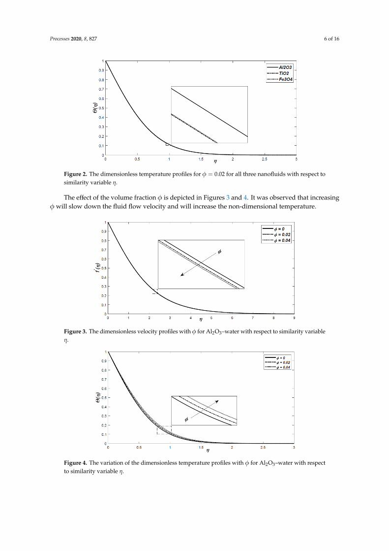
Figure 2. The dimensionless temperature profiles for 𝜙 = 0.02 for all three nanofluids with respect to similarity variable 𝜂.
The effect of the volume fraction 𝜙 is depicted in Figures 3 and 4. It was observed that increasing 𝜙 will slow down the fluid flow velocity and will increase the non-dimensional temperature.
Figure 1. The dimensionless velocity profiles for volume fraction φ = 0.02 for all three nanofluids withrespect to similarity variable η.
Processes 2020, 8, 827 6 of 16
Processes 2020, 8, 827 5 of 16
𝑇(𝑥, 𝑦) = 𝑇 + (𝑇 − 𝑇 )𝜃(𝜂). (21)
Using the fourth-order method (bvp4c) in MATLAB, the system (15) and (16) is solved with conditions (17) and (18), when the nanofluid properties are calculated according to formulas (8)–(11) using the thermophysical values given in Table 1 for Al2O3, TiO2, and Fe3O4 particles, as well as the base fluid of suspension water. Our aim was to investigate the impacts of the volume fraction and nanoparticle’s material type on the heat and mass transfer characteristics.
Figure 1 exhibits the dimensionless velocity distributions for all three nanofluids for 2% additives in the base fluid. It shows that the velocity is greater for Al2O3 than for the other two materials. Figure 2 represents the temperature distribution for the same cases. Here, the Al2O3 also shows greater values than the others.
Figure 1. The dimensionless velocity profiles for volume fraction 𝜙 = 0.02 for all three nanofluids with respect to similarity variable 𝜂.
Figure 2. The dimensionless temperature profiles for 𝜙 = 0.02 for all three nanofluids with respect to similarity variable 𝜂.
The effect of the volume fraction 𝜙 is depicted in Figures 3 and 4. It was observed that increasing 𝜙 will slow down the fluid flow velocity and will increase the non-dimensional temperature.
Figure 2. The dimensionless temperature profiles for φ = 0.02 for all three nanofluids with respect tosimilarity variable η.
The effect of the volume fraction φ is depicted in Figures 3 and 4. It was observed that increasingφ will slow down the fluid flow velocity and will increase the non-dimensional temperature.Processes 2020, 8, 827 6 of 16
Figure 3. The dimensionless velocity profiles with 𝜙 for Al2O3–water with respect to similarity variable 𝜂.
Figure 4. The variation of the dimensionless temperature profiles with 𝜙 for Al2O3–water with respect to similarity variable 𝜂.
The skin friction coefficient and the local Nusselt number is of engineering interest, and these will be presented and discussed in detail. The wall shear stress (𝜏 ) and heat flux (𝑞 ) are defined as 𝜏 = 𝜇 𝜕𝑢𝜕𝑦 , 𝑞 = −𝑘 𝜕𝑇𝜕𝑦 (22)
while the skin friction coefficient (𝐶 ) and the local Nusselt number (𝑁𝑢) are defined as 𝐶 = 𝜏𝜌 𝑈 , 𝑁𝑢 = 𝑥 𝑞𝑘 𝑇 − 𝑇 . (23)
Applying the similarity variables defined in (8) and (9), one gets 𝑅𝑒 / 𝐶 = 1(1 − 𝜙) . 𝑓 (0), 𝑅𝑒 / 𝑁𝑢 = − 𝑘 𝑘 𝜃 (0), (24)
where the local Reynolds number 𝑅𝑒 is defined by 𝑅𝑒 = .
4. Results with CFD Simulations and Discussion
Nowadays, the computation fluid dynamics (CFD) simulation has become an effective tool to predict results in fluid flow characteristics.
The CFD simulations have been performed for the laminar nanofluid flow, according to Figure 5, and Equations (1)–(3) were discretized and solved using ANSYS 18. The sheet was maintained at a constant temperature 𝑇 = 400 K. The fluid flows with constant velocity 𝑈 = 0.01 m/s and the
Figure 3. The dimensionless velocity profiles with φ for Al2O3–water with respect to similarity variableη.
Processes 2020, 8, 827 6 of 16
Figure 3. The dimensionless velocity profiles with 𝜙 for Al2O3–water with respect to similarity variable 𝜂.
Figure 4. The variation of the dimensionless temperature profiles with 𝜙 for Al2O3–water with respect to similarity variable 𝜂.
The skin friction coefficient and the local Nusselt number is of engineering interest, and these will be presented and discussed in detail. The wall shear stress (𝜏 ) and heat flux (𝑞 ) are defined as 𝜏 = 𝜇 𝜕𝑢𝜕𝑦 , 𝑞 = −𝑘 𝜕𝑇𝜕𝑦 (22)
while the skin friction coefficient (𝐶 ) and the local Nusselt number (𝑁𝑢) are defined as 𝐶 = 𝜏𝜌 𝑈 , 𝑁𝑢 = 𝑥 𝑞𝑘 𝑇 − 𝑇 . (23)
Applying the similarity variables defined in (8) and (9), one gets 𝑅𝑒 / 𝐶 = 1(1 − 𝜙) . 𝑓 (0), 𝑅𝑒 / 𝑁𝑢 = − 𝑘 𝑘 𝜃 (0), (24)
where the local Reynolds number 𝑅𝑒 is defined by 𝑅𝑒 = .
4. Results with CFD Simulations and Discussion
Nowadays, the computation fluid dynamics (CFD) simulation has become an effective tool to predict results in fluid flow characteristics.
The CFD simulations have been performed for the laminar nanofluid flow, according to Figure 5, and Equations (1)–(3) were discretized and solved using ANSYS 18. The sheet was maintained at a constant temperature 𝑇 = 400 K. The fluid flows with constant velocity 𝑈 = 0.01 m/s and the
Figure 4. The variation of the dimensionless temperature profiles with φ for Al2O3–water with respectto similarity variable η.
Processes 2020, 8, 827 7 of 16
The skin friction coefficient and the local Nusselt number is of engineering interest, and these willbe presented and discussed in detail. The wall shear stress (τw) and heat flux (qw) are defined as
τw = µn f
(∂u∂y
)y=0
, qw = −kn f
(∂T∂y
)y=0
(22)
while the skin friction coefficient (C f ) and the local Nusselt number (Nu) are defined as
C f =τw
ρb U2 , Nu =x qw
kn f(Tw − Tn f
) . (23)
Applying the similarity variables defined in (8) and (9), one gets
Re1/2x C f =
1
(1−φ)2.5 f ′′ (0), Re−1/2x Nu = −
kn f
kbθ′(0), (24)
where the local Reynolds number Rex is defined by Rex =ρn f Uxµn f
.
4. Results with CFD Simulations and Discussion
Nowadays, the computation fluid dynamics (CFD) simulation has become an effective tool topredict results in fluid flow characteristics.
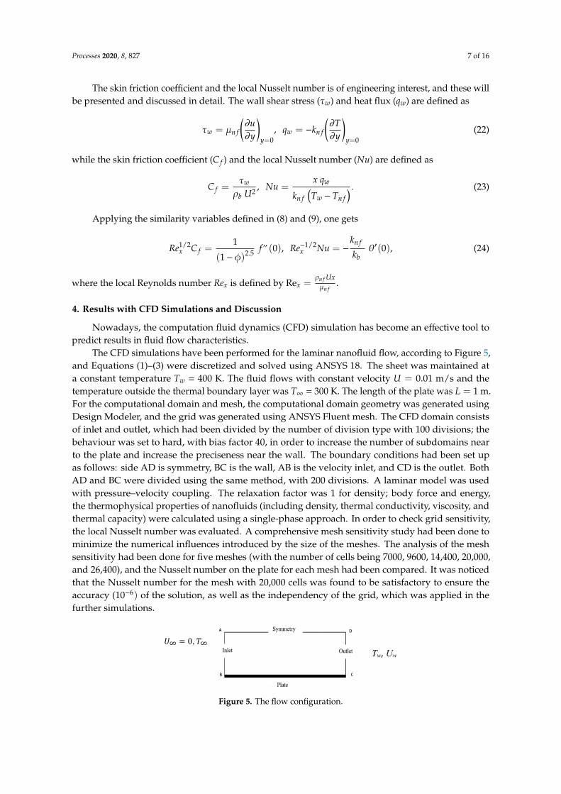
The CFD simulations have been performed for the laminar nanofluid flow, according to Figure 5,and Equations (1)–(3) were discretized and solved using ANSYS 18. The sheet was maintained ata constant temperature Tw = 400 K. The fluid flows with constant velocity U = 0.01 m/s and thetemperature outside the thermal boundary layer was T∞ = 300 K. The length of the plate was L = 1 m.For the computational domain and mesh, the computational domain geometry was generated usingDesign Modeler, and the grid was generated using ANSYS Fluent mesh. The CFD domain consistsof inlet and outlet, which had been divided by the number of division type with 100 divisions; thebehaviour was set to hard, with bias factor 40, in order to increase the number of subdomains nearto the plate and increase the preciseness near the wall. The boundary conditions had been set upas follows: side AD is symmetry, BC is the wall, AB is the velocity inlet, and CD is the outlet. BothAD and BC were divided using the same method, with 200 divisions. A laminar model was usedwith pressure–velocity coupling. The relaxation factor was 1 for density; body force and energy,the thermophysical properties of nanofluids (including density, thermal conductivity, viscosity, andthermal capacity) were calculated using a single-phase approach. In order to check grid sensitivity,the local Nusselt number was evaluated. A comprehensive mesh sensitivity study had been done tominimize the numerical influences introduced by the size of the meshes. The analysis of the meshsensitivity had been done for five meshes (with the number of cells being 7000, 9600, 14,400, 20,000,and 26,400), and the Nusselt number on the plate for each mesh had been compared. It was noticedthat the Nusselt number for the mesh with 20,000 cells was found to be satisfactory to ensure theaccuracy (10−6) of the solution, as well as the independency of the grid, which was applied in thefurther simulations.
Processes 2020, 8, 827 7 of 16
temperature outside the thermal boundary layer was 𝑇 = 300 K. The length of the plate was 𝐿 =1 m. For the computational domain and mesh, the computational domain geometry was generated using Design Modeler, and the grid was generated using ANSYS Fluent mesh. The CFD domain consists of inlet and outlet, which had been divided by the number of division type with 100 divisions; the behaviour was set to hard, with bias factor 40, in order to increase the number of subdomains near to the plate and increase the preciseness near the wall. The boundary conditions had been set up as follows: side AD is symmetry, BC is the wall, AB is the velocity inlet, and CD is the outlet. Both AD and BC were divided using the same method, with 200 divisions. A laminar model was used with pressure–velocity coupling. The relaxation factor was 1 for density; body force and energy, the thermophysical properties of nanofluids (including density, thermal conductivity, viscosity, and thermal capacity) were calculated using a single-phase approach. In order to check grid sensitivity, the local Nusselt number was evaluated. A comprehensive mesh sensitivity study had been done to minimize the numerical influences introduced by the size of the meshes. The analysis of the mesh sensitivity had been done for five meshes (with the number of cells being 7000, 9600, 14,400, 20,000, and 26,400), and the Nusselt number on the plate for each mesh had been compared. It was noticed that the Nusselt number for the mesh with 20,000 cells was found to be satisfactory to ensure the accuracy (10 ) of the solution, as well as the independency of the grid, which was applied in the further simulations.
Figure 5. The flow configuration.
Applying Equations (8)–(11), the effect of volume concentration on the density, viscosity, thermal capacity, and thermal conductivity were determined in [45] for the three nanofluids, with data given in Table 1. It was found that the density and the viscosity increase with 𝜙; however, the thermal capacity and thermal conductivity have opposite behaviour.
Figures 6 and 7 show the impact of the nanoparticles’ material on the dimensional velocity and temperature profiles for 𝜙 = 0.02, respectively. We remark that these figures are in correlation with Figures 1 and 2.
𝑈∞ = 0, 𝑇∞ Tw, Uw
Figure 5. The flow configuration.
Processes 2020, 8, 827 8 of 16
Applying Equations (8)–(11), the effect of volume concentration on the density, viscosity, thermalcapacity, and thermal conductivity were determined in [45] for the three nanofluids, with data given inTable 1. It was found that the density and the viscosity increase with φ; however, the thermal capacityand thermal conductivity have opposite behaviour.
Figures 6 and 7 show the impact of the nanoparticles’ material on the dimensional velocity andtemperature profiles for φ = 0.02, respectively. We remark that these figures are in correlation withFigures 1 and 2.Processes 2020, 8, 827 8 of 16
Figure 6. Velocity profiles perpendicular to the sheet for all three nanofluids; 𝜙 = 0.02.
Figure 7. Temperatures profiles perpendicular to the sheet for all three nanofluids; 𝜙 = 0.02.
The impact of the nanoparticle’s concentration was investigated on Al2O3–water nanofluid in Figures 8 and 9. It follows, according to Figures 3 and 4, that more additives will reduce the velocity and increase the velocity.
0
0.002
0.004
0.006
0.008
0.01
0 0.01 0.02 0.03 0.04
u[m
/s]
y [m]
Al2O3 TiO2 Fe3O4
300
310
320
330
340
350
360
370
380
390
400
0 0.005 0.01 0.015 0.02 0.025 0.03
T [K
]
y [m]
Al2O3 TiO2 Fe3O4
0.004
0.0045
0.005
0.0055
0.006
0.01 0.011 0.012 0.013 0.014 0.015 0.016
304
305
306
307
308
0.011 0.012 0.013 0.014 0.015
Figure 6. Velocity profiles perpendicular to the sheet for all three nanofluids; φ = 0.02.
Processes 2020, 8, 827 8 of 16
Figure 6. Velocity profiles perpendicular to the sheet for all three nanofluids; 𝜙 = 0.02.
Figure 7. Temperatures profiles perpendicular to the sheet for all three nanofluids; 𝜙 = 0.02.
The impact of the nanoparticle’s concentration was investigated on Al2O3–water nanofluid in Figures 8 and 9. It follows, according to Figures 3 and 4, that more additives will reduce the velocity and increase the velocity.
0
0.002
0.004
0.006
0.008
0.01
0 0.01 0.02 0.03 0.04
u[m
/s]
y [m]
Al2O3 TiO2 Fe3O4
300
310
320
330
340
350
360
370
380
390
400
0 0.005 0.01 0.015 0.02 0.025 0.03
T [K
]
y [m]
Al2O3 TiO2 Fe3O4
0.004
0.0045
0.005
0.0055
0.006
0.01 0.011 0.012 0.013 0.014 0.015 0.016
304
305
306
307
308
0.011 0.012 0.013 0.014 0.015
Figure 7. Temperatures profiles perpendicular to the sheet for all three nanofluids; φ = 0.02.
Processes 2020, 8, 827 9 of 16
The impact of the nanoparticle’s concentration was investigated on Al2O3–water nanofluid inFigures 8 and 9. It follows, according to Figures 3 and 4, that more additives will reduce the velocityand increase the velocity.Processes 2020, 8, 827 9 of 16
Figure 8. Velocity profiles perpendicularly to the sheet for Al2O3-water at different volume fractions 𝜙.
Figure 9. Temperatures profiles perpendicular to the sheet for Al2O3–water nanofluid at different volume fractions 𝜙.
The skin friction coefficient and the local Nusselt number were analysed using CFD simulations. Figure 10 exhibits the impact of the nanoparticle’s material on 𝐶 for 𝜙 = 0.02 along the flat surface. We found that the skin friction is higher Fe3O4 than for Al2O3 and TiO2.
0
0.002
0.004
0.006
0.008
0.01
-0.005 0.005 0.015 0.025 0.035 0.045
u[m
/s]
y [m]
Water 0.02 0.04
𝜙
300
310
320
330
340
350
360
370
380
390
400
0 0.005 0.01 0.015 0.02 0.025 0.03
T [K
]
y [m]
0.04 0.02 Water𝜙
0.002
0.0021
0.0022
0.0023
0.0024
0.0025
0.022 0.023 0.024 0.025
Figure 8. Velocity profiles perpendicularly to the sheet for Al2O3-water at different volume fractions φ.
Processes 2020, 8, 827 9 of 16
Figure 8. Velocity profiles perpendicularly to the sheet for Al2O3-water at different volume fractions 𝜙.
Figure 9. Temperatures profiles perpendicular to the sheet for Al2O3–water nanofluid at different volume fractions 𝜙.
The skin friction coefficient and the local Nusselt number were analysed using CFD simulations. Figure 10 exhibits the impact of the nanoparticle’s material on 𝐶 for 𝜙 = 0.02 along the flat surface. We found that the skin friction is higher Fe3O4 than for Al2O3 and TiO2.
0
0.002
0.004
0.006
0.008
0.01
-0.005 0.005 0.015 0.025 0.035 0.045
u[m
/s]
y [m]
Water 0.02 0.04
𝜙
300
310
320
330
340
350
360
370
380
390
400
0 0.005 0.01 0.015 0.02 0.025 0.03
T [K
]
y [m]
0.04 0.02 Water𝜙
0.002
0.0021
0.0022
0.0023
0.0024
0.0025
0.022 0.023 0.024 0.025
Figure 9. Temperatures profiles perpendicular to the sheet for Al2O3–water nanofluid at differentvolume fractions φ.
The skin friction coefficient and the local Nusselt number were analysed using CFD simulations.Figure 10 exhibits the impact of the nanoparticle’s material on C f for φ = 0.02 along the flat surface.We found that the skin friction is higher Fe3O4 than for Al2O3 and TiO2.
Processes 2020, 8, 827 10 of 16Processes 2020, 8, 827 10 of 16
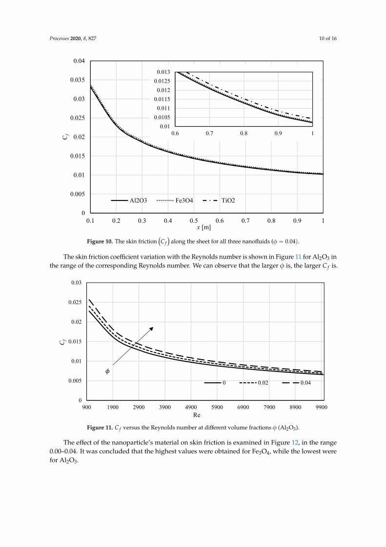
Figure 10. The skin friction (𝐶 ) along the sheet for all three nanofluids (𝜙 = 0.04).
The skin friction coefficient variation with the Reynolds number is shown in Figure 11 for Al2O3
in the range of the corresponding Reynolds number. We can observe that the larger 𝜙 is, the larger 𝐶 is.
Figure 11. 𝐶 versus the Reynolds number at different volume fractions 𝜙 (Al2O3).
The effect of the nanoparticle’s material on skin friction is examined in Figure 12, in the range 0.00–0.04. It was concluded that the highest values were obtained for Fe3O4, while the lowest were for Al2O3.
0
0.005
0.01
0.015
0.02
0.025
0.03
0.035
0.04
0.1 0.2 0.3 0.4 0.5 0.6 0.7 0.8 0.9 1
C f
x [m]
Al2O3 Fe3O4 TiO2
900 1900 2900 3900 4900 5900 6900 7900 8900 99000
0.005
0.01
0.015
0.02
0.025
0.03
Re
C f
0 0.02 0.04
𝜙
0.010.01050.011
0.01150.012
0.01250.013
0.6 0.7 0.8 0.9 1
Figure 10. The skin friction(C f
)along the sheet for all three nanofluids (φ = 0.04).
The skin friction coefficient variation with the Reynolds number is shown in Figure 11 for Al2O3 inthe range of the corresponding Reynolds number. We can observe that the larger φ is, the larger C f is.
Processes 2020, 8, 827 10 of 16
Figure 10. The skin friction (𝐶 ) along the sheet for all three nanofluids (𝜙 = 0.04).
The skin friction coefficient variation with the Reynolds number is shown in Figure 11 for Al2O3
in the range of the corresponding Reynolds number. We can observe that the larger 𝜙 is, the larger 𝐶 is.
Figure 11. 𝐶 versus the Reynolds number at different volume fractions 𝜙 (Al2O3).
The effect of the nanoparticle’s material on skin friction is examined in Figure 12, in the range 0.00–0.04. It was concluded that the highest values were obtained for Fe3O4, while the lowest were for Al2O3.
0
0.005
0.01
0.015
0.02
0.025
0.03
0.035
0.04
0.1 0.2 0.3 0.4 0.5 0.6 0.7 0.8 0.9 1
C f
x [m]
Al2O3 Fe3O4 TiO2
900 1900 2900 3900 4900 5900 6900 7900 8900 99000
0.005
0.01
0.015
0.02
0.025
0.03
Re
C f
0 0.02 0.04
𝜙
0.010.01050.011
0.01150.012
0.01250.013
0.6 0.7 0.8 0.9 1
Figure 11. C f versus the Reynolds number at different volume fractions φ (Al2O3).
The effect of the nanoparticle’s material on skin friction is examined in Figure 12, in the range0.00–0.04. It was concluded that the highest values were obtained for Fe3O4, while the lowest werefor Al2O3.
Processes 2020, 8, 827 11 of 16Processes 2020, 8, 827 11 of 16
Figure 12. The skin friction 𝐶 versus 𝜙 for all three nanofluids.
In Figure 13, the values of 𝑅𝑒 / 𝐶 versus 𝜙 are exhibited for all three additive materials. We remark that the same trends can be seen as in Figure 12.
Figure 13. 𝑅𝑒 / 𝐶 versus 𝜙 for all three nanofluids.
Figure 14 depicts the variation of the Nusselt number along the sheet surface. One can see a slight difference along the x-axis for all three nanofluids when 𝜙 = 0.02. The bigger values for Nu were obtained for Al2O3.
Figure 12. The skin friction C f versus φ for all three nanofluids.
In Figure 13, the values of Re1/2x C f versusφ are exhibited for all three additive materials. We remark
that the same trends can be seen as in Figure 12.
Processes 2020, 8, 827 11 of 16
Figure 12. The skin friction 𝐶 versus 𝜙 for all three nanofluids.
In Figure 13, the values of 𝑅𝑒 / 𝐶 versus 𝜙 are exhibited for all three additive materials. We remark that the same trends can be seen as in Figure 12.
Figure 13. 𝑅𝑒 / 𝐶 versus 𝜙 for all three nanofluids.
Figure 14 depicts the variation of the Nusselt number along the sheet surface. One can see a slight difference along the x-axis for all three nanofluids when 𝜙 = 0.02. The bigger values for Nu were obtained for Al2O3.
Figure 13. Re1/2x C f versus φ for all three nanofluids.
Figure 14 depicts the variation of the Nusselt number along the sheet surface. One can see a slightdifference along the x-axis for all three nanofluids when φ = 0.02. The bigger values for Nu wereobtained for Al2O3.
Processes 2020, 8, 827 12 of 16Processes 2020, 8, 827 12 of 16
Figure 14. The variation of the Nusselt number for all three nanofluids.
The influence of the volume fraction on the local Nusselt number is investigated in Figure 15 for Al2O3 in the range of Reynolds number 900–9000. It can be seen from the figure that the increase in 𝜙 will induce an increase in the Nusselt number as well.
Figure 15. Variation of Nusselt number versus the Reynolds number (Re) for Al2O3–water.
50
70
90
110
130
150
170
190
0.1 0.2 0.3 0.4 0.5 0.6 0.7 0.8 0.9 1
Nu
x [m]
Al2O3 Fe3O4 TiO2
900 1900 2900 3900 4900 5900 6900 7900 8900 99000
20
40
60
80
100
120
140
160
180
Re
Nu
0 0.02 0.04
𝜙
104106108110112114116118
0.4 0.42 0.44 0.46 0.48 0.5
Figure 14. The variation of the Nusselt number for all three nanofluids.
The influence of the volume fraction on the local Nusselt number is investigated in Figure 15 forAl2O3 in the range of Reynolds number 900–9000. It can be seen from the figure that the increase in φwill induce an increase in the Nusselt number as well.
Processes 2020, 8, 827 12 of 16
Figure 14. The variation of the Nusselt number for all three nanofluids.
The influence of the volume fraction on the local Nusselt number is investigated in Figure 15 for Al2O3 in the range of Reynolds number 900–9000. It can be seen from the figure that the increase in 𝜙 will induce an increase in the Nusselt number as well.
Figure 15. Variation of Nusselt number versus the Reynolds number (Re) for Al2O3–water.
50
70
90
110
130
150
170
190
0.1 0.2 0.3 0.4 0.5 0.6 0.7 0.8 0.9 1
Nu
x [m]
Al2O3 Fe3O4 TiO2
900 1900 2900 3900 4900 5900 6900 7900 8900 99000
20
40
60
80
100
120
140
160
180
Re
Nu
0 0.02 0.04
𝜙
104106108110112114116118
0.4 0.42 0.44 0.46 0.48 0.5
Figure 15. Variation of Nusselt number versus the Reynolds number (Re) for Al2O3–water.
Processes 2020, 8, 827 13 of 16
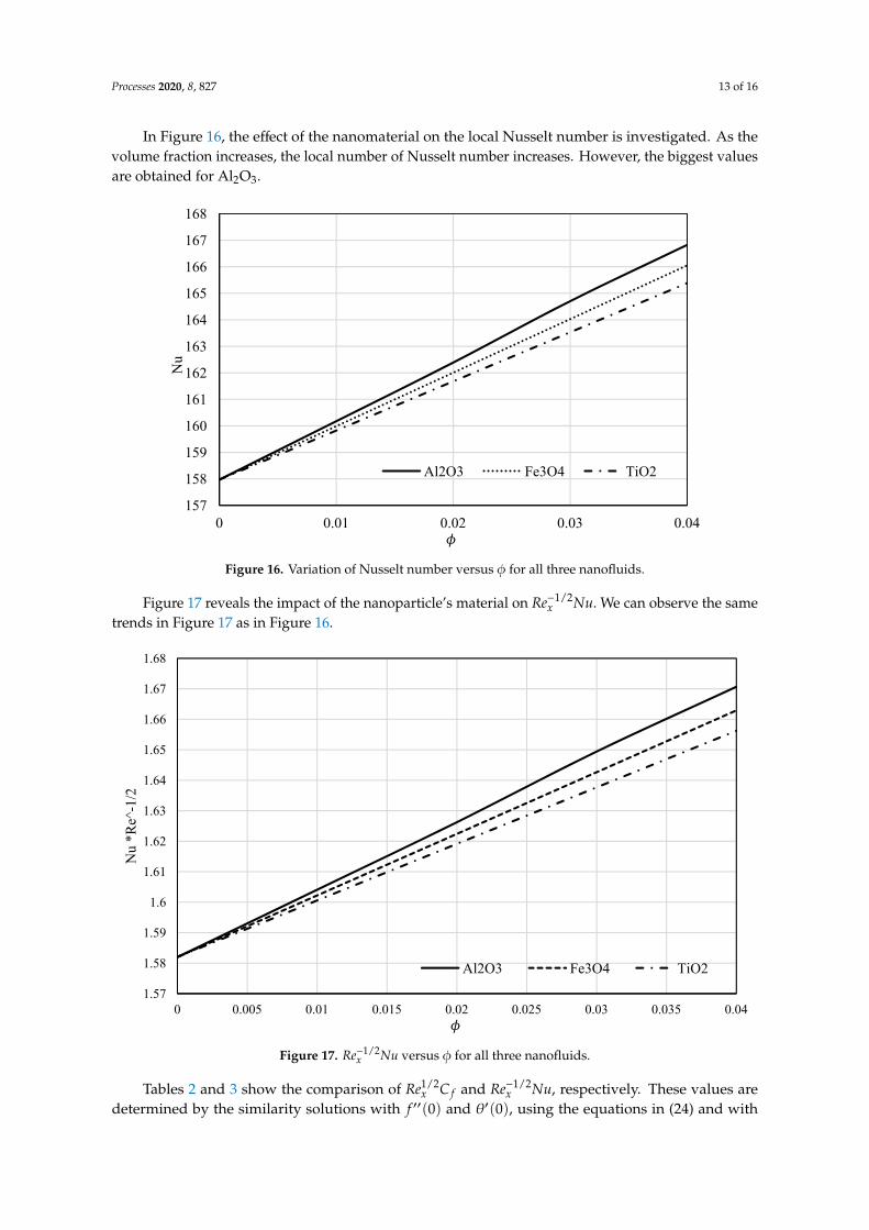
In Figure 16, the effect of the nanomaterial on the local Nusselt number is investigated. As thevolume fraction increases, the local number of Nusselt number increases. However, the biggest valuesare obtained for Al2O3.
Processes 2020, 8, 827 13 of 16
In Figure 16, the effect of the nanomaterial on the local Nusselt number is investigated. As the volume fraction increases, the local number of Nusselt number increases. However, the biggest values are obtained for Al2O3.
Figure 16. Variation of Nusselt number versus 𝜙 for all three nanofluids.
Figure 17 reveals the impact of the nanoparticle’s material on 𝑅𝑒 / 𝑁𝑢. We can observe the same trends in Figure 17 as in Figure 16.
Figure 17. 𝑅𝑒 / 𝑁𝑢 versus 𝜙 for all three nanofluids.
Table 2 and Table 3 show the comparison of 𝑅𝑒 / 𝐶 and 𝑅𝑒 / 𝑁𝑢, respectively. These values are determined by the similarity solutions with 𝑓′′(0) and 𝜃 (0), using the equations in (24) and with CFD simulations as well. We remark that in the range 0.00–0.02 for 𝜙, the values obtained with
0 0.01 0.02 0.03 0.04157
158
159
160
161
162
163
164
165
166
167
168
𝜙
Nu
Al2O3 Fe3O4 TiO2
0 0.005 0.01 0.015 0.02 0.025 0.03 0.035 0.041.57
1.58
1.59
1.6
1.61
1.62
1.63
1.64
1.65
1.66
1.67
1.68
𝜙
Nu
*Re^
-1/2
Al2O3 Fe3O4 TiO2
Figure 16. Variation of Nusselt number versus φ for all three nanofluids.
Figure 17 reveals the impact of the nanoparticle’s material on Re−1/2x Nu. We can observe the same
trends in Figure 17 as in Figure 16.
Processes 2020, 8, 827 13 of 16
In Figure 16, the effect of the nanomaterial on the local Nusselt number is investigated. As the volume fraction increases, the local number of Nusselt number increases. However, the biggest values are obtained for Al2O3.
Figure 16. Variation of Nusselt number versus 𝜙 for all three nanofluids.
Figure 17 reveals the impact of the nanoparticle’s material on 𝑅𝑒 / 𝑁𝑢. We can observe the same trends in Figure 17 as in Figure 16.
Figure 17. 𝑅𝑒 / 𝑁𝑢 versus 𝜙 for all three nanofluids.
Table 2 and Table 3 show the comparison of 𝑅𝑒 / 𝐶 and 𝑅𝑒 / 𝑁𝑢, respectively. These values are determined by the similarity solutions with 𝑓′′(0) and 𝜃 (0), using the equations in (24) and with CFD simulations as well. We remark that in the range 0.00–0.02 for 𝜙, the values obtained with
0 0.01 0.02 0.03 0.04157
158
159
160
161
162
163
164
165
166
167
168
𝜙
Nu
Al2O3 Fe3O4 TiO2
0 0.005 0.01 0.015 0.02 0.025 0.03 0.035 0.041.57
1.58
1.59
1.6
1.61
1.62
1.63
1.64
1.65
1.66
1.67
1.68
𝜙
Nu
*Re^
-1/2
Al2O3 Fe3O4 TiO2
Figure 17. Re−1/2x Nu versus φ for all three nanofluids.
Tables 2 and 3 show the comparison of Re1/2x C f and Re−1/2
x Nu, respectively. These values aredetermined by the similarity solutions with f ′′(0) and θ′(0), using the equations in (24) and with
Processes 2020, 8, 827 14 of 16
CFD simulations as well. We remark that in the range 0.00–0.02 for φ, the values obtained with CFDare slightly greater for both quantities than for the analytical solution obtained with the similaritymethod. However, the difference is small, less than 14.5%, and is especially small (2.7%) for Re1/2
x C fThe difference is due to boundary layer approximations. We consider that the CFD simulation resultscould be closer to the experimental results.
The Sakiadis flow was investigated by determining the velocity and temperature in three types ofnanofluids along a continuously moving sheet surface. The skin friction coefficient and the local Nusseltnumber were calculated. Two methods were used: one of them was analytically applying the traditionalBlasius’ similarity transformation, and solving the obtained coupled ordinary differential equations;the other solution was obtained using CFD simulations. We found that the solid volume fractionsignificantly influences the fluid flow and heat transfer properties. Comparing the three nanoparticles’materials, we note that the Al2O3 has significantly greater thermal conductivity. The larger velocityand temperature values are obtained in the boundary layer for alumina–water fluid than for the othertwo nanomaterials. Increasing the concentration of nanomaterial has produced a decrease in velocityand an increase in temperature in the momentum and thermal boundary layers, respectively. The skinfriction decreases and the Nusselt number increases with the Reynolds number. The values of C f andNu are depicted with the nanoparticle concentration. It was concluded that both linearly increase withφ (see Figures 12 and 16). For Al2O3, the values of the skin friction coefficient are smaller than for titania(TiO2) and magnetite (Fe3O4); conversely, the Nusselt number values are greater than those for theother two materials. It was found that the type of nanofluid is a key factor in improving heat transfer.The behaviour of the skin friction coefficient and the local Nusselt number is like that described byAhmad et al. [31] and Bachok et al. [32]. The simulation results obtained by CFD gave slightly biggervalues for Re1/2
x C f and Re−1/2x Nu, which indicates that the skin friction should be slightly higher in
reality than the value calculated, according to boundary layer theory.
Author Contributions: G.B.: conceptualization, methodology, investigation, formal analysis, and writing—originaldraft preparation; M.K.: methodology, investigation, numerical simulation, data curation, and writing—review andediting; K.H.: methodology, investigation, numerical simulation, data curation, and writing—review and editing.All authors have read and agreed to the published version of the manuscript.
Processes 2020, 8, 827 15 of 16
Funding: This work was supported by Project No. 129257 and implemented with support provided from theNational Research, Development and Innovation Fund of Hungary, financed under the K_18 funding scheme andGINOP-2.3.4-15-2016-00004 project, which aims to promote cooperation between higher education and industry,is supported by the European Union and the Hungarian State, and is co-financed by the European RegionalDevelopment Fund interest.
Conflicts of Interest: The authors declare no conflict of interest.
References
1. Prandtl, L. Über Flüssigkeitsbewegungen bei sehr kleiner Reibung. In Vier Abhandlungen zur Hydromechanikund Aerodynamik; Prandtl, L., Betz, A., Eds.; Universitatsverlag Göttingen: Göttingen, Germany, 2010;pp. 484–494.
2. Blasius, H. Grenzschichten in Flüssigkeiten mit kleiner Reibung. Z. Angew. Math. Phys. 1909, 56, 1–37.3. Schlichting, H. Boundary Layer Theory, 8th ed.; Springer: New York, NY, USA, 2020; ISBN 3540662707/978-3540662709.4. Altan, T.; Oh, S.; Gegel, G. Metal Forming Fundamentals and Applications; ASM International: Cleveland, OH,
USA, 1983.5. Fisher, E.G. Extrusion of Plastics; Wiley: New York, NY, USA, 1976.6. Tadmor, Z.; Gogos, C. Principles of Polymer Processing; Wiley: New York, NY, USA, 1979.7. Sakiadis, B.C. Boundary-layer behaviour on continuous solid surfaces: I. Boundary-layer equations for
two-dimensional and axisymmetric flow. AIChE J 1961, 7, 26–28. [CrossRef]8. Tsou, F.; Sparrow, E.; Goldstein, R. Flow and heat transfer in the boundary layer on a continuous moving
surface. Int. J. Heat Mass Transf. 1967, 10, 219–235. [CrossRef]9. Crane, L.J. Flow past stretching plate. Z. Angew. Math. Phys. 1970, 21, 645–647. [CrossRef]10. Chakrabarti, A.; Gupta, A.S. Hydromagnetic flow and heat transfer over a stretching sheet. Q. Appl. Math.
1979, 37, 73–78. [CrossRef]11. Banks, W.H.H. Similarity solutions of the boundary layer equations for a stretching wall. JMecT 1983, 2,
375–392.12. Bognár, G.V. On similarity solutions of boundary layer problems with upstream moving wall in
non-Newtonian power-law fluids. IMA J. Appl. Math. 2011, 77, 546–562. [CrossRef]13. Bognár, G.V.; Csáti, Z. Numerical Solution to Boundary Layer Problems over Moving Flat Plate in
Non-Newtonian Media. J. Appl. Math. Phys. 2014, 2, 8–13. [CrossRef]14. Bognár, G.V. Numerical method for the boundary layer problems of non-Newtonian fluid flows along
moving surfaces. Electron. J. Qual. Theory Differ. Equations 2016, 1–11. [CrossRef]15. Haider, S.; Butt, A.S.S.; Li, Y.-Z.; Imran, S.M.; Ahmad, B.; Tayyaba, A. Study of entropy generation with
multi-slip effects in MHD unsteady flow of viscous fluid past an exponentially stretching surface. Symmetry2020, 12, 426. [CrossRef]
16. Mahabaleshwar, U.S.; Kumar, P.V.; Nagaraju, K.R.; Bognár, G.; Nayakar, S.N.R. A new exact solution for theflow of a fluid through porous media for a variety of boundary conditions. Fluids 2019, 4, 125. [CrossRef]
17. Andersson, H.I. MHD flow of a viscoelastic fluid past a stretching surface. Acta Mech. 1992, 95, 227–230.[CrossRef]
18. Tonekaboni, S.A.M.; Abkar, R.; Khoeilar, R. On the Study of Viscoelastic Walters’ B Fluid in Boundary LayerFlows. Math. Probl. Eng. 2012, 2012, 1–18. [CrossRef]
19. Siddheshwar, P.; Mahabaleshwar, U.; Chan, A. MHD flow of walters’ liquid b over a nonlinearly stretchingsheet. Int. J. Appl. Mech. Eng. 2015, 20, 589–603. [CrossRef]
20. Singh, J.; Mahabaleshwar, U.S.; Bognar, G. Mass transpiration in nonlinear MHD flow due to porousstretching sheet. Sci. Rep. 2019, 9, 1–15. [CrossRef]
21. Takhar, H.S.; Nitu, S.; Pop, I. Boundary layer flow due to a moving plate: Variable fluid properties. Acta Mech.1991, 90, 37–42. [CrossRef]
22. Pop, I.; Gorla, R.S.R.; Rashidi, M. The effect of variable viscosity on flow and heat transfer to a continuousmoving flat plate. Int. J. Eng. Sci. 1992, 30, 1–6. [CrossRef]
23. Elbashbeshy, E.M.A.; Bazid, M.A.A. The effect of temperature-dependent viscosity on heat transfer over acontinuous moving surface. J. Phys. Appl. Phys. 2000, 33, 2716–2721. [CrossRef]
24. Andersson, H.I.; Aarseth, J.B. Sakiadis flow with variable fluid properties revisited. Int. J. Eng. Sci. 2007, 45,554–561. [CrossRef]
Processes 2020, 8, 827 16 of 16
25. Choi, S.U.S. Enhancing thermal conductivity of fluids with nanoparticles. In Proceedings of the 1995ASME International Mechanical Engineering. Congress and Exposition, San Francisco, CA, USA,12–17 November 1995; pp. 99–105.
26. Das, S.K.; Choi, S.U.S.; Yu, W.; Pradet, T. Nanofluids: Science and Technology; Wiley: Hoboken, NJ, USA, 2007.27. Xuan, Y.; Li, Q. Heat transfer enhancement of nanofluids. Int. J. Heat Fluid Flow 2000, 21, 58–64. [CrossRef]28. Wong, K.V.; De Leon, O. Applications of nanofluids: Current and future. Adv. Mech. Eng. 2010, 2, 519659.
[CrossRef]29. Raza, J.; Mebarek-Oudina, F.; Mahanthesh, B. Magnetohydrodynamic flow of nano Williamson fluid
generated by stretching plate with multiple slips. Multidiscip. Model. Mater. Struct. 2019, 15, 871–894.[CrossRef]
30. Ibrahim, W. Magnetohydrodynamic (MHD) boundary layer stagnation point flow and heat transfer of ananofluid past a stretching sheet with melting. Propuls. Power Res. 2017, 6, 214–222. [CrossRef]
31. Ahmad, S.; Rohni, A.M.; Pop, I. Blasius and Sakiadis problems in nanofluids. Acta Mech. 2010, 218, 195–204.[CrossRef]
32. Bachok, N.; Ishak, A.; Pop, I. Flow and heat transfer characteristics on a moving plate in a nanofluid. Int. J.Heat Mass Transf. 2012, 55, 642–648. [CrossRef]
33. Gingold, H. Modelling fluid flow over solid surfaces. Int. J. Model. Identif. Control. 2014, 21, 237. [CrossRef]34. Liepmann, H.W. Investigations on Laminar Boundary-Layer Stability and Transition on Curved Boundaries; NACA
Wartime Report; National Advisory Committee for Aeronautics: Washington, DC, USA, May 1946.35. Janour, Z. Resistance of a Plate in Parallel Flow at Low Reynolds Number; NACA Technical Memorandum;
National Advisory Committee for Aeronautics: Washington, DC, USA, November 1953.36. Schaaf, S.A.; Sherman, F.S. Skin Friction in Slip Flow. J. Aeronaut. Sci. 1954, 21, 85–90. [CrossRef]37. Farniya, A.A.; Esplandiu, M.J.; Bachtold, A. Sequential Tasks Performed by Catalytic Pumps for Colloidal
Crystallization. Langmuir 2014, 30, 11841–11845. [CrossRef]38. Niu, R.; Palberg, T. Seedless assembly of colloidal crystals by inverted micro-fluidic pumping. Soft Matter
2018, 14, 3435–3442. [CrossRef]39. Kudenatti, R.B.; Misbah, N.-E. Hydrodynamic flow of non-Newtonian power-law fluid past a moving wedge
or a stretching sheet: A unified computational approach. Sci. Rep. 2020, 10, 9445. [CrossRef]40. Rasool, G.; Shafiq, A.; Khalique, C.M.; Zhang, T. Magnetohydrodynamic Darcy–Forchheimer nanofluid flow
over a nonlinear stretching sheet. Phys. Scr. 2019, 94, 105221. [CrossRef]41. Dero, S.; Rohni, A.M.; Saaban, A. MHD micropolar nanofluid flow over an exponentially stretching/shrinking
surface: Triple solutions. J. Adv. Res. Fluid Mech. Therm. Sci. 2019, 56, 165–174.42. Khan, S.A.; Nie, Y.; Ali, B. Multiple Slip Effects on Magnetohydrodynamic Axisymmetric Buoyant Nanofluid
Flow above a Stretching Sheet with Radiation and Chemical Reaction. Symmetry 2019, 11, 1171. [CrossRef]43. Ali, B.; Nie, Y.; Khan, S.A.; Sadiq, M.T.; Tariq, M. Finite Element Simulation of Multiple Slip Effects on MHD
Unsteady Maxwell Nanofluid Flow over a Permeable Stretching Sheet with Radiation and Thermo-Diffusionin the Presence of Chemical Reaction. Processes 2019, 7, 628. [CrossRef]
44. Oztop, H.F.; Abu-Nada, E. Numerical study of natural convection in partially heated rectangular enclosuresfilled with nanofluids. Int. J. Heat Fluid Flow 2008, 29, 1326–1336. [CrossRef]
45. Klazly, M.; Bognár, G. CFD study for the flow behaviour of nanofluid flow over flat plate. Int. J. Mech. 2020,14, 49–57.