EUROGRAPHICS 2016 / J. Jorge and M. Lin (Guest Editors) Volume 35 (2016), Number 2 Narrow Band FLIP for Liquid Simulations Florian Ferstl 1 , Ryoichi Ando 2 , Chris Wojtan 2 , Rüdiger Westermann 1 , and Nils Thuerey 1 1 Technische Universität München 2 IST Austria Figure 1: Two simulations with a (background-)grid resolution of 200 3 : Our method (left) is nearly indistinguishable from regular FLIP (right), but uses only one million particles instead of 24 million. Computations outside of the pressure solver are sped up by a factor of more than 6, the total computation time for 250 frames is reduced from 4.4h to 2h, and the average memory footprint is reduced by a factor of 2. Abstract The Fluid Implicit Particle method (FLIP) for liquid simulations uses particles to reduce numerical dissipation and provide important visual cues for events like complex splashes and small-scale features near the liquid surface. Unfortunately, FLIP simulations can be computationally expensive, because they require a dense sampling of particles to fill the entire liquid volume. Furthermore, the vast majority of these FLIP particles contribute nothing to the fluid’s visual appearance, especially for larger volumes of liquid. We present a method that only uses FLIP particles within a narrow band of the liquid surface, while efficiently representing the remaining inner volume on a regular grid. We show that a naïve realization of this idea introduces unstable and uncontrollable energy fluctuations, and we propose a novel coupling scheme between FLIP particles and regular grid which overcomes this problem. Our method drastically reduces the particle count and simulation times while yielding results that are nearly indistinguishable from regular FLIP simulations. Our approach is easy to integrate into any existing FLIP implementation. Categories and Subject Descriptors (according to ACM CCS): I.3.7 [Computer Graphics]: Three-Dimensional Graphics and Realism—Animation 1. Introduction The Fluid Implicit Particle method (FLIP) is arguably the most widely used simulation algorithm for high-quality liquid special ef- fects [BLMB13, BBAW15]. Impressive large-scale effects ranging from characters splashing in the ocean to flooding cities have been simulated with this method. Its main strengths result from lever- aging non-diffusive Lagrangian transport in combination with ac- curate Eulerian discretizations to ensure divergence-freeness. The particles in a FLIP simulation also provide important visual cues for events like complex splashes and small-scale features near the liquid surface. Unfortunately, FLIP simulations can be computationally expen- sive, as they require a dense sampling of the fluid domain with par- ticles. Furthermore, the vast majority of these FLIP particles con- tribute nothing to the fluid’s visual appearance, especially for larger volumes of liquid. We present a method that only uses FLIP particles within a nar- c 2016 The Author(s) Computer Graphics Forum c 2016 The Eurographics Association and John Wiley & Sons Ltd. Published by John Wiley & Sons Ltd.
Transcript
EUROGRAPHICS 2016 / J. Jorge and M. Lin(Guest Editors)
Volume 35 (2016), Number 2
Narrow Band FLIP for Liquid Simulations
Florian Ferstl1, Ryoichi Ando2, Chris Wojtan2, Rüdiger Westermann1, and Nils Thuerey1
1Technische Universität München 2IST Austria
Figure 1: Two simulations with a (background-)grid resolution of 2003: Our method (left) is nearly indistinguishable from regular FLIP(right), but uses only one million particles instead of 24 million. Computations outside of the pressure solver are sped up by a factor of morethan 6, the total computation time for 250 frames is reduced from 4.4h to 2h, and the average memory footprint is reduced by a factor of 2.
AbstractThe Fluid Implicit Particle method (FLIP) for liquid simulations uses particles to reduce numerical dissipation and provideimportant visual cues for events like complex splashes and small-scale features near the liquid surface. Unfortunately, FLIPsimulations can be computationally expensive, because they require a dense sampling of particles to fill the entire liquid volume.Furthermore, the vast majority of these FLIP particles contribute nothing to the fluid’s visual appearance, especially for largervolumes of liquid. We present a method that only uses FLIP particles within a narrow band of the liquid surface, while efficientlyrepresenting the remaining inner volume on a regular grid. We show that a naïve realization of this idea introduces unstableand uncontrollable energy fluctuations, and we propose a novel coupling scheme between FLIP particles and regular gridwhich overcomes this problem. Our method drastically reduces the particle count and simulation times while yielding resultsthat are nearly indistinguishable from regular FLIP simulations. Our approach is easy to integrate into any existing FLIPimplementation.
Categories and Subject Descriptors (according to ACM CCS): I.3.7 [Computer Graphics]: Three-Dimensional Graphics andRealism—Animation
1. Introduction
The Fluid Implicit Particle method (FLIP) is arguably the mostwidely used simulation algorithm for high-quality liquid special ef-fects [BLMB13, BBAW15]. Impressive large-scale effects rangingfrom characters splashing in the ocean to flooding cities have beensimulated with this method. Its main strengths result from lever-aging non-diffusive Lagrangian transport in combination with ac-curate Eulerian discretizations to ensure divergence-freeness. Theparticles in a FLIP simulation also provide important visual cues
for events like complex splashes and small-scale features near theliquid surface.
Unfortunately, FLIP simulations can be computationally expen-sive, as they require a dense sampling of the fluid domain with par-ticles. Furthermore, the vast majority of these FLIP particles con-tribute nothing to the fluid’s visual appearance, especially for largervolumes of liquid.
We present a method that only uses FLIP particles within a nar-
row band of the liquid surface, while efficiently representing the re-maining inner body of the fluid on a regular grid. Although the mainidea may seem straightforward, its implementation is non-trivial,and the naïve approach introduces unstable and uncontrollable en-ergy fluctuations. Our method drastically reduces the particle countand simulation times, while still exhibiting the desired bounded en-ergy behavior and yielding results that are nearly indistinguishablefrom regular FLIP simulations.
The contributions of our method are:• A method to efficiently reduce the number of particles in a FLIP
simulation, leading to speed-ups up to a factor of 5 in our exam-ples (factor 2 in average), and• Insights into instabilities caused by naïve couplings between par-
ticle and grid velocities, leading to a stable narrow band ap-proach.
In this way, we achieve significant performance improvements withan approach that can be easily integrated into any existing FLIPimplementation.
1.1. Related Work
Researchers in computer graphics use a variety of methods for sim-ulating fluid dynamics. Eulerian discretizations are popular becausethey avoid complicated re-meshing of Lagrangian meshes andneighbor-finding between Lagrangian particles, and they can takeadvantage of fast methods for indexing and caching data in regu-lar grids [FM96, Sta99, FF01]. However, Eulerian methods tend toeither suffer from CFL conditions or numerical diffusion from con-tinual re-sampling operations. On the other hand, Lagrangian fluidsimulation techniques, such as smoothed particle hydrodynamics(SPH) [MCG03, IOS∗14] avoid continual re-sampling operationsat the expense of stability restrictions, neighborhood searches, andnumerical smoothing over the radius of a pre-defined kernel. We re-fer the reader to [Bri08] for a more thorough look at fluid dynamicsresearch in computer graphics.
Our method is based on an Eulerian-Lagrangian hybrid methodcalled the fluid-implicit particle method (FLIP), which was intro-duced to the graphics community by Zhu and Bridson [ZB05]. TheFLIP method has also been used for fluid control [PHT∗13] andtwo-phase flow [BB12, ATW15]. Note that our narrow band ap-proach is actually used by Ando et al. [ATW15]. In addition, pre-vious researchers have improved upon the FLIP method by cor-recting particle positions [UBH14] or adapting grid and particlesizes [ATW13]. Ando et al. [ATT12] use directed particle inser-tion in combination with particle merging and splitting to simulatethin liquid sheets, effectively using a higher FLIP particle densitynear the liquid surface than in the liquids interior. Adaptive particlesizes have also been used in purely Lagrangian approaches, e.g., bySolenthaler and Gross [SG11].
Several other approaches have taken advantage of hybrid meth-ods in order to leverage the strengths of both Eulerian and La-grangian fluid discretizations. Several authors [SS06, LTKF08,RWT11] were able to successfully combine SPH simulations withregular grid-based simulations, while Cornelis et al. [CIPT14] useSPH particles for the pressure projection step of a FLIP simulation.The material point method (MPM) combines a grid-based Eule-rian simulation with Lagrangian marker particles in order to model
a wider range of elastoplastic materials such as snow [SSC∗13]or viscoelastic fluids and foams [RGJ∗15, YSB∗15]. Golas etal. [GNS∗12] use Lagrangian particles as a vortex basis in the inte-rior of a grid-based Eulerian simulation. For the related problem ofsurface tracking, Enright et al. [ELF05] augment the Eulerian levelset method with Lagrangian marker particles placed on both sidesof a tracked surface, in order to better preserve Lagrangian detailswhile letting the grid handle topological changes. Their method issimilar to our tracking of the liquids surface, yet we only requireLagrangian particles on one side of the surface.
Recently, Chentanez et al. [CMK14] coupled a 3D Eulerianmethod, a 2D Eulerian shallow water solver, and a Lagrangian SPHdiscretization within the same simulation. Their approach of com-puting an SPH simulation near the surface of an Eulerian solver issimilar in spirit to ours, but their approach focuses solely on SPH,not FLIP. Additionally, in our experience, even a non-trivial adop-tion of their method to pure FLIP simulations leads to inherentlyunstable simulations. The analysis and solution of this problem is acentral contribution of our paper.
2. FLIP
Our liquid simulation solves the inviscid Navier-Stokes equations
∂u∂t
=−u ·∇u− 1ρ∇p+ f,
which are subject to the incompressibility constraint ∇·u = 0.Here, u denotes the liquid’s velocity field, p the internal pressure,ρ the density and f represents acceleration due to external forcesacting on the liquid. In the following, normal and bold variablesrepresent parameters and variables stored on a regular grid, whilevariables with the subscript i refer to quantities stored on particles.Variables with the superscript p refer to particle quantities mappedto the grid.
We will briefly review a typical FLIP approach, before detail-ing our narrow band algorithm. In a time step of the regular FLIPalgorithm, the particles are first passively advected using the gridvelocity u. Then, the velocity stored on the particles is mapped tothe grid, yielding a velocity field up which covers the whole fluiddomain and which is stored as an intermediate velocity field u∗. Ina similar manner, a particle region is reconstructed on the grid inthe form of a scalar field φ
p, whose zero-contour encloses all par-ticles. This φ
p is used in the remaining steps as level set function φ
to mark the location of the liquid surface. The external forces areadded, u∗ is projected and the velocity of every particle i is updatedaccording to the formula
ui← (1−α) uPICi +α uFLIP
i . (1)
Here, uPICi is the current grid velocity, and uFLIP
i is the differencebetween the current velocity and the velocity right after mappingthe particles to the grid, both interpolated at the position of particlei. The parameter α∈ [0;1] controls the amount of velocity diffusionin the simulation, and can be related to the fluid viscosity. It is ad-visable to use some form of particle re-sampling to avoid extremelydensely and/or sparsely sampled regions. In its simplest form, thisre-sampling adds and removes particles where necessary to keepthe per-cell particle count in a chosen range. We do not perform
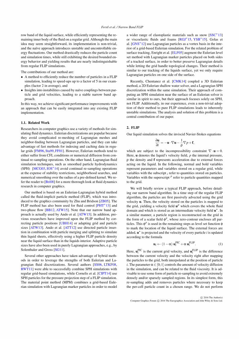
this re-sampling in cells at the liquid surface to prevent visual arti-facts. In our implementation we use α = 0.95, in combination withtri-linear weights (i.e., a tri-linear kernel function) to map particledata to the grid, and vice versa. Fig. 2 (with statements colored red)summarizes the regular FLIP algorithm described above.
In principle, FLIP particles are relatively cheap: In contrast toparticles in, e.g., SPH, there is no communication between theparticles themselves, and particle solely communicate via the un-derlying grid. Also, FLIP particles typically do not carry a massand are passively advected with the flow. Hence, they are very ro-bust against variations in sampling density, and can be removedand added without much overhead. However, in practice, the sheeramount of particles that is required to run a full FLIP simula-tion leads to a huge computational workload—typically, eight par-ticles are used per cell in three dimensions [Bri08, BB12], butfewer [BB08] or even more [GB13] particles have also been usedsuccessfully. In all our examples (see Section 4), the computationsinvolving FLIP particles take up more than 60% of the compu-tation time in each simulation step when using a standard, pre-conditioned conjugate gradients solver. This ratio increases fur-ther for advanced variations of FLIP, e.g., when a position correc-tion step is performed to ensure a more uniform particle distribu-tion [ATT12, UBH14].
3. Narrow band FLIP
The central idea of our approach is to use FLIP particles only in anarrow band of fixed width R inside of the liquid surface, and to usea standard, grid-based simulation with semi-Lagrangian advectionin the interior of the domain. Hence, we refer to our method asnarrow band FLIP (NB-FLIP). Our narrow band method consistsof three main components:
1. The coupling of grid simulation and FLIP simulation.2. A surface tracking method for correctly handling the liquids in-
terior.3. The re-sampling of particles to maintain a narrow band of fixed
width.
The green statements in Fig. 2 highlight that few changes are neces-sary to turn a standard FLIP simulation into a NB-FLIP simulation.
Throughout our algorithm, we make use of a level set functionφ. In contrast to standard FLIP, we need information about the dis-tance of particles to the liquid surface. However, because φ is notour main visual representation, it does not need to be overly ac-curate, and we initialize a Manhattan distance with several quickpasses over the grid. As a consequence, the reduced amount of par-ticles in NB-FLIP easily compensates for the additional cost of thelevel set, as well as for other additional steps that our method intro-duces.
Our choice to restrict particles to the surface region can be fur-ther motivated by comparing FLIP velocity fields with their counterparts in pure grid-based simulations. We observe that differencesbetween the velocity fields—advected via FLIP particles on the onehand, and advected using a semi-Lagrangian scheme on the otherhand—are predominantly noticeable near the surface. The impactof the FLIP particles is strongest right at the surface and quickly de-creases away from it, which is illustrated in Fig. 3. This effect can
1: Advect particles2: [NB-FLIP] Advect u and φ on grid⇒ u′ and φ
′
3: Map particles to grid⇒ φp and up
4: Update level set and velocity on grid[FLIP] φ← φ
Figure 2: Comparison of the time step algorithms for FLIP andNB-FLIP. Steps tagged with [FLIP] and [NB-FLIP] are unique toFLIP and NB-FLIP, respectively. Untagged steps are common toboth methods.
be observed independently of the order of the employed advectionscheme. Rather, it is a result of the inherent differences between thebackward semi-Lagrangian advection and the forward FLIP advec-tion. Close to the surface, these differences are amplified throughhigh frequencies in the underlying velocity fields and through theuse of approximate, extrapolated velocities outside of the liquid’ssurface.
A comparison of the memory requirements for a regular FLIPsimulation versus a pure Eulerian simulation indicates the mem-ory savings that can potentially be achieved with our method: EachFLIP particle has to store at least position and velocity (3 floatseach). Assuming 8 particles per cell, this leads to a memory re-quirement of 48 floating point numbers per cell. In contrast, whenusing a purely Eulerian representation, the required information percell is a single velocity and a level-set value (4 floats in total). Thus,in all areas where our method can switch to the grid based repre-sentation, memory is reduced by a factor of 12.
3.1. Grid-particle coupling
The FLIP simulation in the narrow band has to be properly coupledwith the grid simulation in the liquids interior: First, we advect thegrid velocity u on the whole liquid domain by performing a semi-Lagrangian advection step, which yields an advected grid velocityu′. Similarly, we advect all FLIP particles and map them to the grid,which in turn yields an advected particle velocity up. Finally, at allgrid vertices where a particle velocity is available (i.e., where up isvalid), we combine the values of u′ and up into a single velocityu∗. At all remaining grid vertices, we set u∗ equal to u′. The com-bination of up and u′ should ensure a full FLIP simulation near theliquid surface, i.e., values of up should completely overwrite val-ues of u′ in the interior of the narrow band as well as at the surfaceitself. In addition to that, the transition from grid to narrow band iscrucial, and therefore has to be handled properly. To demonstratethat a naive transition can quickly lead to unphysical gains in mo-mentum, we will first present an erroneous combination rule thatis based on ideas from existing methods, and, afterwards, we willpresent our “fixed” combination rule.
Figure 3: Comparison of semi-Lagrangian and grid-based advec-tion for two timesteps of a 2D simulation. Shown is a color codingof ||u′−up||/||u||: the difference between u′ and up (velocity ad-vected with a semi-Lagrangian scheme and FLIP particles, respec-tively), relative to the magnitude of the velocity u (see Fig. 2).
Several previous works deal with particle/grid couplings. Theone most closely related to ours is the method by Chentanez etal. [CMK14], in which SPH particles at the surface are coupledwith a grid-based, semi-Lagrangian simulation. A smooth transi-tion from grid to particles is realized based on the ratio betweena grid density and a particle density. Since we do not use a vari-able density formulation, we adapt this to our case by only com-puting a single density on the grid, i.e., a non-physical particle den-sity ρ
p ≥ 0. At each grid vertex, we determine ρp by summing up
the kernel weights of all contributing, neighboring FLIP particles,and then calculate a combined velocity from up and u′ at everyface F = (i+ 1
2 , j,k) of the staggered grid. In line with previouswork, an intuitive, yet unfortunately erroneous formulation for thiscombination is given by:
u∗F ← lerp(u′F , up
F , t), with t = min
(1,
ρpF
ρpmax
). (2)
Here, ρpmax is a constant threshold, which we set to 1 in all our
experiments, and lerp(a,b, t) = a+ t · (b−a) is the linear interpo-lation operator. Eq. (2) is analogously applied to the y- and z-components of the velocity, which are stored at the correspondinglyoriented faces of the staggered grid.
As we will outline below, the combined velocity calculated withEq. (2) leads to inherently unstable simulations and cannot be usedin practice. Note that in the SPH-coupling approach by Chentanezet al. [CMK14], the FLIP coefficient α (see Eq. (1)) is varied basedon the distance to the liquid surface in addition to mixing particleand grid velocities. In our experiments, this variation did not causesignificant differences other than increasing the amount of numer-ical diffusion (because of smaller values for α), and hence we donot use this variant. For the same reason, we found it unnecessaryto employ their proposed temporal filtering of transition weights.
The problem with the density-based combination of Eq. (2) oc-
Frame 1common
Frame 170NB-FLIP with Eq. (2)
Frame 170NB-FLIP with Eq. (3)
Frame 170FLIP
0 100 200 300 4000
20
40
60
Frame
Kin
etic
ener
gyNB-FLIP with Eq. (2)NB-FLIP with Eq. (3)FLIP
Figure 4: Comparison of velocity combination variants: (Top) Foursnapshots of a 323 simulation of surfaces waves. (Bottom) Plot ofthe corresponding kinetic energies. While NB-FLIP with Eq. (2)generates artificial momentum, NB-FLIP with Eq. (3) is almostidentical to standard FLIP, and the surface correctly comes to rest.
curs at the transition of the narrow band to the inner volume. Gridvertices located just outside of the narrow band —i.e., verticeswhose distance to the liquid surface is larger than the narrow bandwidth R—can receive contributions from the narrow-band particles.Effectively, this means that particle velocities are extrapolated intothe interior grid region, which results in relatively large differencesbetween up and u′ (compared to the interior of the narrow band).In practice, these differences lead to a consistent over-estimationof the fluid motion. Amplified by the non-dissipative nature of theFLIP simulation in the narrow band, they typically accumulate tolarge errors over time.
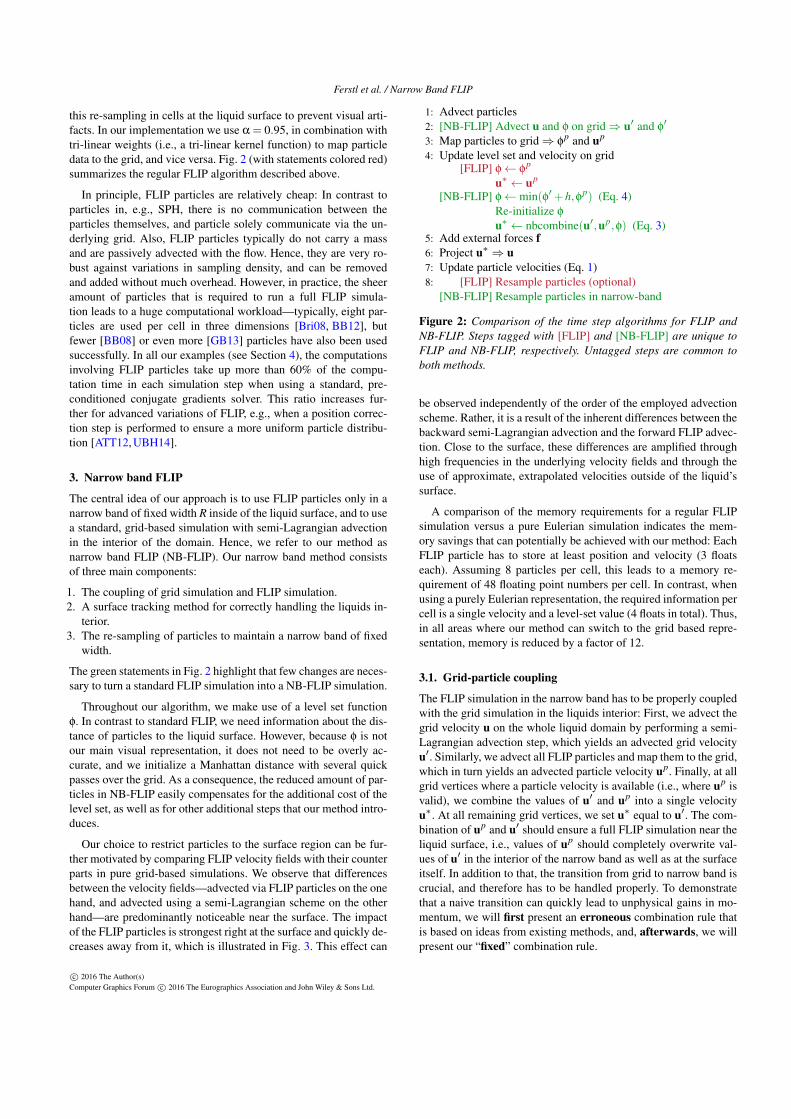
To overcome this problem, we make the combination dependenton the distance of the grid vertices to the surface, which ensuresthat no extrapolated particle velocities are used in the interior ofthe liquid. While the narrow band has a width of R, we only usethe particle velocities up in a thinner band of width r < R, whichis illustrated in Fig. 6. Because we found, that a smooth transitionbetween grid and particle velocities does not increase the quality of
Figure 5: Surface tracking and particle re-sampling in NB-FLIP: FLIP particles (orange dots), zero-contour of the level set φ (blue, filled)and zero-contour of the mapped particle region φ
p (orange, contour only) during one time step of our algorithm (see Fig. 2). Note that φp is
only shown for illustration purposes in (a+e) and is not actually computed after re-sampling.
the simulation, we use a sharp transition between up and u′. Thisresults in the following “fixed” combination rule, which is referredto as nbcombine(u′,up,φ) in Fig. 2:
u∗F ←{
upF , if φF ≥−r
u′F , else. (3)
The distance r should be chosen depending on the narrow bandwidth R. The choice of R, in turn, is a performance trade-off, withNB-FLIP becoming identical to FLIP if R→∞. Let h denote thewidth of one cell. Then, where not stated otherwise, we use a nar-row band width of R = 3h, and, because we use a tri-linear interpo-lation kernel, we choose r to be one cell smaller, i.e., r = 2h.
Fig. 4 compares both versions and illustrates the importanceof the velocity transition. The unphysical behavior produced byEq. (2) is obvious in the energy plot even for this simplified setup.For more complex scenarios this approach quickly leads to overlyviolent and unstable liquid motions. In contrast, our transition func-tion using Eq. (3) yields the expected behavior and produces resultsthat are very close to a regular FLIP simulation (Fig. 4 bottom left).Animations of these cases can be found in the accompanying video.
φ
0
−h
−r
−R
Nar
row
band
Com
bina
tion
band
Res
ampl
ing
band
Figure 6: Breakdown of the narrow band: FLIP particles are main-tained in a band of width R inside of the liquid surface, but theirvelocities only contribute to vertices in a “combination band” ofwidth r < R (see Eq. (3)). Particles are only added/removed in a“resampling band” with minimum distance h to the surface, in or-der to prevent changes to the liquid surface.
3.2. Surface tracking
In standard FLIP, the whole liquid domain is covered by particles,which makes surface tracking straightforward. Compared to that, inNB-FLIP, particles are missing in the liquids interior, and the insideand outside of the narrow band cannot be distinguished withoutadditional information. Therefore, to keep track of the particle-freeregions that belong to the liquids interior, we use the level set φ.
We initialize φ and a corresponding band of particles directlyfrom analytical object descriptions or meshes. The substeps of onesurface advection step (see Fig. 2) are illustrated in Fig. 5. We startby advecting φ, which yields an advected level set φ
′, and map theadvected particles to the grid, yielding a level set φ
p of the narrowband particles. The zero-contour of φ
′ and the outer zero-contourof φ
p (which corresponds to the liquid surface) are similar, but notequal. Since we want to obtain a tracking scheme that is equivalentto standard FLIP, the particle surface should “overrule” the levelset surface. Therefore, we shrink the surface of the level set φ
′ bythe width of one cell h, and then compute its union with φ
p. Moreprecisely, we compute the level set of the next time step as
φ←min(φ′+h,φp). (4)
In principle, this method works if the maximum distance error,i.e., the distance between the surfaces corresponding to φ
′ and φp,
is less than h. Thin liquid features are completely sampled withparticles, and are always treated correctly. To ensure a small dis-tance error, we use a 4th order Runge-Kutta scheme to compute theforward- and back-traces required for advection. In practice, oursurface tracking works well even for time steps with a CFL numberof 5 and higher. Note that, for stability reasons, we do not shrinkthe level set surface by a distance larger than h. This is becauseexcessive shrinking can lead to spurious holes beneath the narrowband which are hard to fix.
3.3. Particle re-sampling
In order to maintain a narrow band of fixed width R, we re-samplethe particles at the end of each time step. Our re-sampling is basedon a minimum number n of particles per cell (we use n = 8). First,we remove all particles outside of the narrow band, i.e., particleswhose distance to the liquid surface is larger than R, and ensure thatno more than 2n particles are present per cell by removing excess
particles. Likewise, we add new particles in cells where less than nparticles are present, whose velocities are initialized with the cur-rent grid velocity. Since the liquid surface should not be changedwhen adding or removing particles, we never add or remove parti-cles at positions that are less than one cell width h away from thesurface, i.e. particles are only re-sampled where−R≤ φ≤−h (seeFig. 6).
As a consequence of the particle re-sampling in the narrow bandin combination with our surface tracking, the volume conservationof our method is equivalent to regular FLIP, i.e., we do not conservemass exactly. The level set representation in the liquids interior im-plicitly conserves mass and the particle density in the narrow bandis kept uniform. Hence, significant changes in mass can only origi-nate right at the liquid’s surface.
4. Results
We have implemented our method in two FLIP simulation frame-works: a basic, light-weight solver [PT15], and a more complexone with advanced FLIP techniques [ATT12]. Both implementa-tions use eight particles per grid cell, as well as a standard conju-gate gradients solver with modified incomplete Cholesky precondi-tioner for the projection step. Detailed runtimes and particle num-bers for the following simulations can be found in Table 1. For thelight-weight solver, we additionally specify the average memoryfootprint of the running simulation in the last column (“Avg. Mem-ory”). We used narrow band widths of R = 3h and R = 4h (withr = R− 1), both of which we have found to be a good compro-mise between performance and memory consumption on the onehand and simulation quality on the other hand. Thinner bands canbe problematic because the particles only have an influence in asmaller portion of the full narrow band (see Fig. 6), while slightlythicker bands do not offer significant gains in simulation quality.
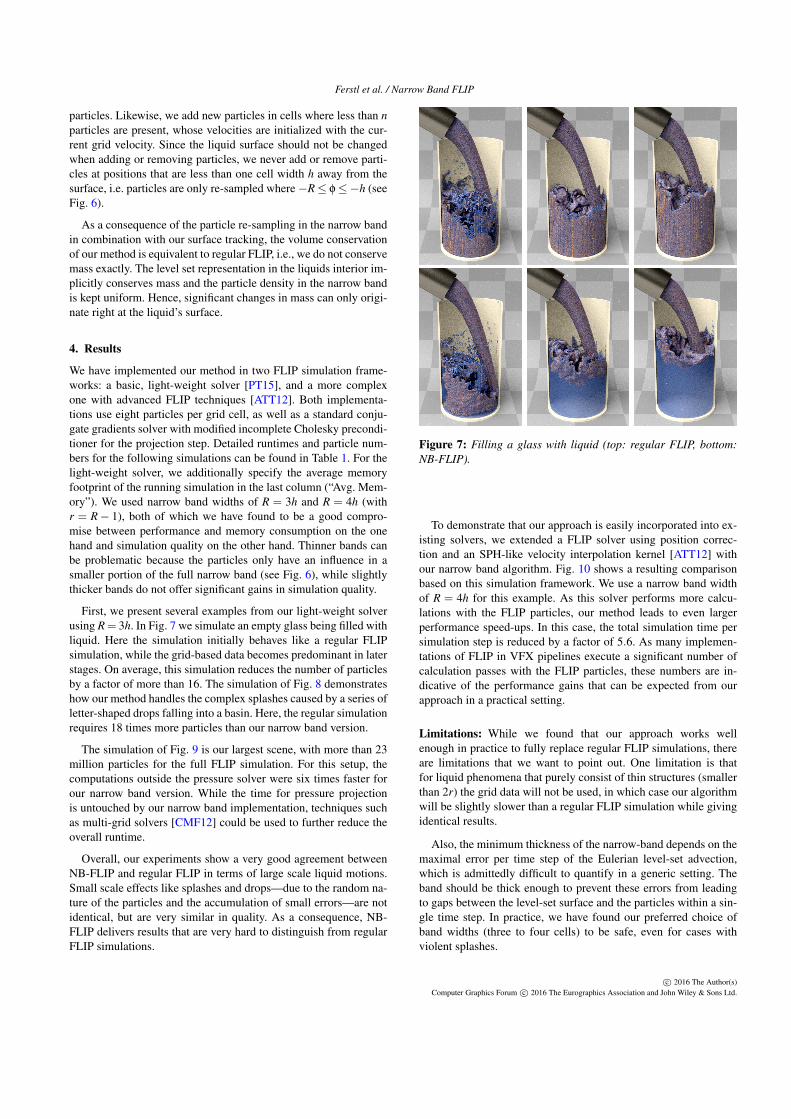
First, we present several examples from our light-weight solverusing R = 3h. In Fig. 7 we simulate an empty glass being filled withliquid. Here the simulation initially behaves like a regular FLIPsimulation, while the grid-based data becomes predominant in laterstages. On average, this simulation reduces the number of particlesby a factor of more than 16. The simulation of Fig. 8 demonstrateshow our method handles the complex splashes caused by a series ofletter-shaped drops falling into a basin. Here, the regular simulationrequires 18 times more particles than our narrow band version.
The simulation of Fig. 9 is our largest scene, with more than 23million particles for the full FLIP simulation. For this setup, thecomputations outside the pressure solver were six times faster forour narrow band version. While the time for pressure projectionis untouched by our narrow band implementation, techniques suchas multi-grid solvers [CMF12] could be used to further reduce theoverall runtime.
Overall, our experiments show a very good agreement betweenNB-FLIP and regular FLIP in terms of large scale liquid motions.Small scale effects like splashes and drops—due to the random na-ture of the particles and the accumulation of small errors—are notidentical, but are very similar in quality. As a consequence, NB-FLIP delivers results that are very hard to distinguish from regularFLIP simulations.
Figure 7: Filling a glass with liquid (top: regular FLIP, bottom:NB-FLIP).
To demonstrate that our approach is easily incorporated into ex-isting solvers, we extended a FLIP solver using position correc-tion and an SPH-like velocity interpolation kernel [ATT12] withour narrow band algorithm. Fig. 10 shows a resulting comparisonbased on this simulation framework. We use a narrow band widthof R = 4h for this example. As this solver performs more calcu-lations with the FLIP particles, our method leads to even largerperformance speed-ups. In this case, the total simulation time persimulation step is reduced by a factor of 5.6. As many implemen-tations of FLIP in VFX pipelines execute a significant number ofcalculation passes with the FLIP particles, these numbers are in-dicative of the performance gains that can be expected from ourapproach in a practical setting.
Limitations: While we found that our approach works wellenough in practice to fully replace regular FLIP simulations, thereare limitations that we want to point out. One limitation is thatfor liquid phenomena that purely consist of thin structures (smallerthan 2r) the grid data will not be used, in which case our algorithmwill be slightly slower than a regular FLIP simulation while givingidentical results.
Also, the minimum thickness of the narrow-band depends on themaximal error per time step of the Eulerian level-set advection,which is admittedly difficult to quantify in a generic setting. Theband should be thick enough to prevent these errors from leadingto gaps between the level-set surface and the particles within a sin-gle time step. In practice, we have found our preferred choice ofband widths (three to four cells) to be safe, even for cases withviolent splashes.
Figure 8: A series of letter-shaped drops hitting a pool of liquid using narrow-band FLIP requiring 18× fewer particles.
5. Conclusions
We have described a novel approach to significantly reduce thenumber of FLIP particles. Our algorithm readily integrates into ex-isting FLIP solvers and can result in up to 22× fewer particles. Thisreduction factor strongly depends on the scenario, but especiallyfor large volumes and advanced FLIP simulation approaches it canlead to speed-up factors larger than 5 without degrading simulationquality.
In addition to performance gains our approach has the potentialto significantly reduce the amount of data that needs to be stored onhard disk (up to the aforementioned factor of 12). This is highly in-teresting for VFX productions, as legal requirements typically dic-tate that all data of a shot be available long after completion. Itwill be interesting future work to combine our approach with moreaggressive compressions schemes to further reduce storage require-ments.
Acknowledgements
This work was supported by the European Union under the ERCAdvanced Grant 291372 SaferVis and the ERC Starting Grants637014 realFlow and 638176 BigSplash.
References[ATT12] ANDO R., THUEREY N., TSURUNO R.: Preserving fluid sheets
with adaptively sampled anisotropic particles. IEEE Trans. on Visualiza-tion and Computer Graphics 18 (8) (2012), 1202–1214. 2, 3, 6, 7
[ATW13] ANDO R., THUEREY N., WOJTAN C.: Highly adaptive liquidsimulations on tetrahedral meshes. ACM Transactions on Graphics 32,4 (2013), 103:1–103:10. 2
[ATW15] ANDO R., THUEREY N., WOJTAN C.: A stream functionsolver for liquid simulations. ACM Transactions on Graphics 34, 4(2015), 53:1–53:9. 2
[BB08] BATTY C., BRIDSON R.: Accurate viscous free surfaces forbuckling, coiling, and rotating liquids. In Symposium on Computer Ani-mation (2008), pp. 219–228. 3
[BB12] BOYD L., BRIDSON R.: MultiFLIP for energetic two-phase fluidsimulation. ACM Trans. on Graphics 31, 2 (2012), 16:1–16:12. 2, 3
[BBAW15] BAILEY D., BIDDLE H., AVRAMOUSSIS N., WARNER M.:Distributing liquids using OpenVDB. In ACM SIGGRAPH 2015 Talks(2015), ACM, pp. 285:1–285:1. 1
[BLMB13] BUDSBERG J., LOSURE M., MUSETH K., BAER M.: Liq-uids in “The Croods”. In Digital Prod. Symp. (DigiPro) (2013). 1
[Bri08] BRIDSON R.: Fluid Simulation for Computer Graphics. AK Pe-ters/CRC Press, 2008. 2, 3
[CIPT14] CORNELIS J., IHMSEN M., PEER A., TESCHNER M.: IISPH-FLIP for incompressible fluids. Computer Graphics Forum 33, 2 (2014),255–262. 2
[CMK14] CHENTANEZ N., MÜLLER M., KIM T.: Coupling 3D Eule-rian, heightfield and particle methods for interactive simulation of largescale liquid phenomena. In Symp. Comp. Anim. (2014), pp. 1–10. 2, 4
[ELF05] ENRIGHT D., LOSASSO F., FEDKIW R.: A fast and accuratesemi-Lagrangian particle level set method. Computers & Structures 83,6-7 (2005), 479–490. 2
[FF01] FOSTER N., FEDKIW R.: Practical animation of liquids. In ACMProc. Comp. Graphics and Interactive Techniques (2001), pp. 23–30. 2
[FM96] FOSTER N., METAXAS D.: Realistic animation of liquids.Graph. Models and Img. Proc. 58, 5 (1996), 471–483. 2
Figure 9: Several frames of a breaking dam hitting a row of cylinders (top: regular FLIP, bottom: NB-FLIP).
Figure 10: Stills generated with a different implementation: the underlying FLIP solver performs significantly more calculations with theparticles, leading to a speed-up for our narrow band approach of 5.6×. The FLIP particles are color coded according to their position.
[GB13] GERSZEWSKI D., BARGTEIL A. W.: Physics-based animationof large-scale splashing liquids. ACM Transactions on Graphics 32, 6(2013), 185:1–185:6. 3
[GNS∗12] GOLAS A., NARAIN R., SEWALL J., KRAJCEVSKI P.,DUBEY P., LIN M.: Large-scale fluid simulation using velocity-vorticitydomain decomposition.ACM Trans. Graph. 31, 6(2012), 148:1–148:9. 2
[IOS∗14] IHMSEN M., ORTHMANN J., SOLENTHALER B., KOLB A.,TESCHNER M.: SPH fluids in computer graphics. In Eurographics -State of the Art Reports (2014), pp. 21–42. 2
[LTKF08] LOSASSO F., TALTON J., KWATRA N., FEDKIW R.: Two-way coupled SPH and particle level set fluid simulation. IEEE Trans. onVisualization and Computer Graphics 14, 4 (2008), 797–804. 2
[MCG03] MÜLLER M., CHARYPAR D., GROSS M.: Particle-based fluidsimulation for interactive applications. In Symposium on Computer Ani-mation (2003), pp. 154–159. 2
[PHT∗13] PAN Z., HUANG J., TONG Y., ZHENG C., BAO H.: Interac-tive localized liquid motion editing. ACM Transactions on Graphics 32,6 (2013), 184:1–184:10. 2
[RGJ∗15] RAM D., GAST T., JIANG C., SCHROEDER C., STOMAKHIN
A., TERAN J., KAVEHPOUR P.: A material point method for viscoelas-tic fluids, foams and sponges. In Symposium on Computer Animation(2015), pp. 157–163. 2
[RWT11] RAVEENDRAN K., WOJTAN C., TURK G.: Hybrid smoothedparticle hydrodynamics. In Symp. on Comp. Anim. (2011), pp. 33–42. 2
[SS06] SUÁREZ N., SUSÍN A.: A mesh-particle model for fluid anima-tion. In Ibero-American Symposium in Computer Graphics (2006). 2
[SSC∗13] STOMAKHIN A., SCHROEDER C., CHAI L., TERAN J.,SELLE A.: A material point method for snow simulation. ACM Trans-actions on Graphics 32, 4 (2013), 102. 2
[UBH14] UM K., BAEK S., HAN J.: Advanced hybrid particle-gridmethod with sub-grid particle correction. Computer Graphics Forum33, 7 (Oct. 2014), 209–218. 2, 3
[YSB∗15] YUE Y., SMITH B., BATTY C., ZHENG C., GRINSPUN E.:Continuum foam: A material point method for shear-dependent flows.ACM Transactions on Graphics 34, 5 (Nov. 2015), 160:1–160:20. 2
[ZB05] ZHU Y., BRIDSON R.: Animating sand as a fluid. ACM Trans-actions on Graphics 24, 3 (2005), 965–972. 2