NASA Contractor Report 3 5 8 0 A Comparative Study of Soviet vs. Western Helicopters Part 2 - Evaluation of Weight, Maintainability, and Design Aspects of Major Components W. 2. Stepniewski and R. A. Shim CONTRACT NAS2- 10062 MARCH 1983 funsn https://ntrs.nasa.gov/search.jsp?R=19830010378 2018-08-25T14:04:56+00:00Z
Transcript
NASA Contractor Report 3 5 8 0
A Comparative Study of Soviet vs. Western Helicopters
Part 2 - Evaluation of Weight, Maintainability, and Design Aspects of Major Components
A Comparative Study of Soviet vs. Western Helicopters
Part 2 - Evaluation of Weight, Maintainability, and Design Aspects of Major Components
W. 2. Stepniewski International Technical Associates, Ltd. Upper Darby, Pennsylvania
R. A. Shinn Aeromechanics Laboratory A VRADCOM Research and Technology Laboratories Ames Research Center Moffett Field, Calzfornia
Prepared for Aeromechanics Laboratory AVRADCOM Research and Technology Laboratories Ames Research Center under Contract NASZ- 10062
National Aeronautics and Space Administration
Scientific and Technical information Branch
1983
1.1 Objectives.. .............................................. 1 1.2 Comparison of Weight-Prediction Methods. .......................... 1 1.3 Selection of Helicopters for Comparison ............................ 9 1.4 Evaluation of Component Design Aspects ........................... 10 1.5 Rating of Helicopter Configurations by Tishchenko, et al ................. 11
Inaoduction...............................................lO 8 Relative Weights of Major Components ............................. 109 Relative Major Component Weight Trends for Various Configurations. ........ 13 1 Maintenance Comparison - Soviet and Western Helicopters. ............... 143 Evaluation of the Rotor System Design. ............................ 150
When the outline of “The Comparative Study of Soviet vs. Western Helicopters” was first being formulated, it was contemplated that in addition to the general comparison of the rotorcraft as a whole contained in Part I, it would be desirable to obtain a deeper insight into the design philosophies of the major components of the compared aircraft.
However, it soon became apparent that a complete study aIong those lines would grow into an awesome task exceeding the intended scope and volume content of the project. Furthermore, much of the technical information required for such an undertaking was simply not available, at least as far as Soviet helicopters were concerned.
Consequently, it was decided to limit the component comaprison to the following: (1) Weights - In addition to ascertaining the various trends regarding the weights of the major components, three methods of weight-prediction (one Soviet and two Western) were critically examined, and the results were compared to the actual weights. (2) Maintainability - Although the scope of this investigation is limited chiefly due to the lack of verifiable information on Soviet helicopters, it is believed that there is good authority for the approach to the maintainability aspects regarding differences and commonalities exhibited by the two schools of design. (3) Evaluation of the overaIl component design - The design evaluation technique used in this study represents an initial attempt to develop a quantitative method for judging and comparing the design merits of the components. Because of its preliminary nature, this task was limited to illustrating the proposed approach on the examples of main-rotor blades and hubs.
In the book “Helicopters - Selection of Design Parameters” by Tishchenko et al, which is used frequently as a reference, configurations of large transport helicopters were rated in the following order regarding their payload-carrying capabilities: first, single rotor; second, side-by-side; and third, tandem. A thorough critical examination of that rating system would grow into a design and sizing study. However, by showing that the relative weight trends of major helicopter components constitute first-order inputs with respect to placement in a particular class, it was possible to show that if the relative-weight trends exhibited by Western designs rather than those considered by Tishchenko, et al were applied, the tandem would probably excel in relative payload capabilities when compared with the single-rotor configuration.
As in the case of Part I, “General Comparison of Designs,” this evaluation was prepared with the assistance of various individuals and organizations. In this respect, the authors and associate editor wish to express their gratitude to Dr. R.M. Carlson, Director of the U.S. Army Aviation Research and Technology Labs for his encouragement and valuable suggestions. Thanks are also due to Dr. M.P. Scully of the same organization; and to Messrs. R.H. Swan, A.H. Schmidt, and J.S. Wisniewski from Boeing Vertol for their valuable contributions. Finally, it should be noted that Mr. R.A. Shinn, who served as monitor of Part I of this project, also served as coauthor of this volume, while Mr. W.D. Mosher of the U.S. Army Aviation Research and Technology Labs served as monitor of Part II. Mrs. Wanda L. Metz, associate editor, was also responsible for the composition of both parts of this study.
W.Z. Stepniewski R. A. Shinn
Upper Darby, Pa. USA July 30, 1982
vi
AR
a
CF
Cl
chp
D
Fbr
F cb
F CP
F cr
50 FF
Gr I ramp
Z r/g I. S’P
Kt
k
/?*
kb
kd
k mad
kr
L
Lc L rw
M
N ref
aspect ratio
adjustment factor, also design coefficient
centrifugal force, lb or m.ton
constant accounting for such fuel items as auxiliary fuel system, pressurization, and inflight fueling
crashworthiness and survivability factor for the fuel system
blade chord; ft or m
horsepower; in metric units
diameter; ft
fuel tanks and supporting structure tolerance factor
factor denoting the type of flight control operating mechanism
flight coneol ballistic tolerance factor
crashworthiness factor (fuel tanks)
lubrication oil-system factor
fuel flow; Ib/hr
total fuel tank capacity; gal
factor denoting ramp presence
landing-gear retraction factor
factor denoting blade stiffness inplane influence on skid landing gears
configuration factor (single rotor = 1.0; tandem rotor = 1.3)
direct weight coefficient
indirect weight coefficient
coefficient related to number of blades
drag coefficient
design coefficient, where m = material; a = design; and d = development stage
rotor-type coefficient
fuselage length; ft
cabin length from nose to end of cabin floor; ft
rampwell length; ft
moment, or torque; ft-lb or kg-m
total installed referred horsepower, in chp
vii
n number
crash load factor
limit load factor (at design gross weight)
landing load factor
ultimate Ioad factor
“I p wgr X n,fl(Wgr)mex
“21 E wgr X qj f/t wgr)m ax
rotor radius; ft or m
R G R/76m
radius of blade attachment fittings; ft
revolutions per minute
fuselage wetted area; ft2 or m2
shaft horsepower; hp or chp
specific weight; psf
power to i-pm ratio
blade thickness at 25% R; ft
flight velocity; kn
tip speed; fps or m/s
weight; lb or kg
actual weight; lb or kg
gross weight; lb or kg
hovering gross weight; lb or kg
predicted weight; lb or kg
relative component weight, W E Wcn/Wgr
relative payload, WpI e Wp,/Wgr
zero-range relative payload (weight output), Wplo E Wp,,/Wgr
disc loading; psf or kg/m2
number of stages in main-rotor drive
“c/f
“If
nllf
“u/r
“I
“II
R
R
r
rpm
Sf
SUP
SW
T
t
V
vr W
W* W gr W grh
WP
W
W PI
WPkl
W
.?
a
QlA
‘ya ACG
h
h
configuration coefficient
blade-type coefficient
nonuniform torque coefficient
center of gravity range at Wgr ; ft
blade aspect ratio
X = Aj78
. . . Vlll
A0 V
a
si
8d
ar
BY
b
bc
bg bl
c
CC
elf
cn
des
dr
ds
dsh
w em
eng
eq
. .
ew0 f
fc
fs
f s-r fr
fu
fw
gb
grr h
hr
igb
blade reference aspect ratio
first natural blade frequency in flap bending, per rev
rotor solidity
Subscripts (unless called otherwise in parts of complete symbols)
air induction airduct air outlet average number of blades boosted controls body group blade(s) cowling cockpit controls crash load factor component number(s) design drive drive system drive shaft electrical group engine mounts engine(s) equivalent equipment other equipment fuselage flight controls fuel system fuel system less tank fuel tank(s) fuel wetted area gearbox tail-rotor gearbox hub horizontal tail intermediate gearbox
k7 mrx
mc
mgb mr
mrc
msc
”
n-c
nw
PI
pmr
Pss ref
rfc
rsc
r/g rot
S
sbs
sh
sP sr
ss
TO
ran
rot
rr
rrr
u/r
vr
W
WI
z
landing gear maximum manual controls main-rotor gearbox main rotor main-rotor controls main-rotor system & hydraulics nacelles nacelle less cowling wetted nacelle(s) payload per main rotor propulsion subsystem referred rotor flight controls rotor system controls landing-gear retraction rotor skid side-by-side shaft(s) swashplate single rotor subsystem takeoff tandem total tail rotor transmission rating ultimate vertical tail wheel wheel-type landing-gear legs summation, or overall
ix
chapter 1
Introductory Considerations
1 .l Objectives
As a follow-up to the general comparison of the helicopter designs performed in Part I of this
study, Part II is devoted to a comparative analysis of the major components of Soviet vs. Western
helicopters.
In principle, it would be desirable to examine in some detail the following aspects of major com-
ponents:
(a) conceptual design approach (b) maintainability and producibility (c) weight-prediction methods, and actual weight trends.
However, with the limited knowledge available regarding current Soviet helicopters, it would be
difficult, or almost impossible, to perform a comprehensive, in-depth analysis of items (a) and (b).
With respect to weight aspects, the situation is much better since, in Ref. 1, not only are the weight
prediction formulae given for major components - presumably used by the most prominent Soviet
helicopter designers as represented by the team headed by Tishchenko - the actual weights of the
components are also given for several in-production Soviet helicopters. Taking advantage of this infor-
mation, it is possible to conduct a more comparative analysis of the weight aspects of the major heli-
copter components on a higher level than of the design concepts, and producibility and maintainability.
Consequently, the bulk of this volume will be devoted to weight aspects, and only a limited evaluation
will be afforded to the other items.
1.2 Comparison of Weight Prediction Methods
Soviet Formulae. As mentioned in the preceding section, one can find all the formulae necessary
for the prediction of the weights in Ref. 1. These formulae are summarized in Table 1.1-T. which was
reproduced from Ref. 1, and then individually evaluated in Ch. 2.
Western Formulae. With respect to selecting Western counterparts for Soviet formulae, one must
take into consideration that almost every major American and European helicopter company as well
as most government agencies have their own preferred weight-prediction methods, some of which are
considered proprietary. In view of this, it was decided to use two sets of weight-prediction formulae; one of which is represented by the method used by Boeing Vertol (Table l.l-BV), and the other that
used by the Research and Technology Laboratories (RTL) of the U.S. Army Aviation R&D Command
(Table l.l-RTL).
TABL
E 1.
1-T
SUM
MAR
Y O
F SO
VIET
WEI
GH
T FO
RM
ULA
E
N
.- -
HEL
ICO
PTER
C
OM
PON
ENT
1.
MAI
N
RO
TOR
BL
ADES
I
2.
MAI
N
RO
TOR
H
UB
AND
H
ING
ES
3.
TAIL
R
OTO
R
GR
OU
P:
a.
Tail
Rot
or
Blad
es
b.
Tail
Rot
or
Hub
4.
FUSE
LAG
E (w
ith
cow
lings
)
5.
LAN
DIN
G
GEA
R
6.
DR
IVE
SYST
EM
a.
Mai
n G
earb
oxes
(W
/atta
chm
ent
& lu
bric
ant)
b.
Angu
lar
Inte
rmed
iate
G
earb
oxes
(W
/lubr
ican
t)
c.
Tail-
Rot
or
Gea
rbox
(W
/lubr
ican
t)
d.
Tran
smis
sion
Sh
aft
WEI
GH
T FO
RM
ULA
E
(at
Vr =
22
0mls
=
‘721
.82
fps)
nb/
wb/
=
k;cb
j (d?”
/
x0”
) [ 1
+
aAR
t -
A,,)]
wh
= k:
kn
b,
nb/
(CFb
,) 1.
35
nbltr
W
b/rr
= k:
lrr
[an R
tf”/(&
IO.’ 1
‘h
tr =
k;,“b
/,,[7
+
oeo5
(nb/
, -
4)](c
Fb,,)
1’35
w f
* 0.
25
= kf
‘g
r Sf
0.88
L0
.16(
l +
a)
‘lg
= kl
g ‘g
r
W m
gb
= kf
,gbn
mgb
(ada
v )o
’8
wjg
b =
k :g
b njg
b boM
eq
)‘**
For
twin
-roto
r he
licop
ters
:
M w
=
776.
2(SH
Pror
/ns~
kp
m)s
h 0)
For
sing
le-ro
tor
helic
opte
rs: M w
=
776.
2(H
P,,/(
rpm
),h)
W trg
b =
k:rg
bMrro
e8
whe
re
Mtr
= 71
6.2(
HPr
r/rpm
rr)
W sh
=
ksh
Lsh
vu,&
) 2’
3
TABL
E 1.
1-T
(Con
t’d)
7.
FUEL
SY
STEM
8.
PRO
PULS
ION
SU
BSYS
TEM
S
(with
en
gine
mou
nt,
cool
ing
syst
em,
lubr
ican
t,
lubr
icat
ion
syst
em,
and
fire
supp
ress
ion
syst
em
9.
FLIG
HT
CO
NTR
OL
GR
OU
P
a.
Boos
ted
Con
trols
(s
was
hpla
te,
cont
rols
fro
m
boos
ters
, hy
drau
lic
syst
em o
f lif
ting
roto
rs)
b.
Man
ual
Con
trols
(in
cl.
auxi
liary
bo
osts
)
wbc
=
kbcn
b,C
’
For
twin
-roto
r co
nfig
urat
ion:
W m
c =
k,.,,
, L
For
sing
le-ro
tor
conf
igur
atio
n:
W m
c =
k,,R
w
TABL
E 1 .
l-BV
SUM
MAR
Y O
F BO
EIN
G-V
ERTO
L W
EIG
HT
FOR
MU
LAE
P
HEL
ICO
PTER
C
OM
PON
ENT
1.
MAI
N
RO
TOR
BL
ADES
2.
MAI
N
RO
TOR
H
UB
AND
H
ING
ES
3.
TAIL
R
OTO
R
GR
OU
P
4.
FUSE
LAG
E:
a.
Body
G
roup
(in
cl.
verti
cal
& ve
ntra
l ta
ils)
b.
Hor
izon
tal
Tail
c.
Engi
ne M
ount
s
d.
Engi
ne N
acel
le S
truct
ure
e.
Air
Indu
ctio
n
5.
LAN
DIN
G
GEA
R
6.
DR
IVE
SYST
EM:
a.
Prim
ary
and
Auxi
liary
b.
Tail
Rot
or
7.
FUEL
SY
STEM
WEI
GH
T FO
RM
ULA
?),,w
b/ =
44
U[(7
0-4W
g,)~
,f(0.
07/?
2)
O.I(
R-r&
Ck,
(R
1*6/
kdt)1
0~43
8
W,
= 67
a [W
b,R
(rpm
)2m
r(HPm
r)?‘8
2nb~
.5km
e~
70-”
lo*3
58
Wt,
= 74
.2a[
r:;25
(0
.07
HP,
,)o*5
0.0
7 v,
& 7t
?rrn
b,trC
tr]0*
67
‘bg
= 72
5a{
[(70m
4 W
g,)n
u,,(7
0-3S
f)(Lc
, +
L,,
+ AC
G)
]o.5
log v
,,)
O.*
‘ht
= $&
d,,t
W em
=
“eng
( ‘
eng
“c/f
)o’4
’
‘n
= ne
ng
%
kn
‘ei
= ne
ng
Den
g La
d ka
i
Yg
= k/
g W
gr
(wdd
mr=
250
am,[(
HPm
r/rpm
m,)z
m~~
25kt
]0*6
7
(Wdl
)t,
= JO
Out
, [7.
7(H
P,,/r
pm,)]
0.
8
Wfs
=
kfs
Wfu
TABL
E 1 .
l-BV
(Con
t’d)
8.
PRO
PULS
ION
SU
BSYS
TEM
S
a.
Engi
ne E
xhau
st S
yste
m
b.
Engi
ne C
oolin
g
c.
Engi
ne C
ontro
ls
d.
Engi
ne S
tarti
ng
e.
Engi
ne L
ubric
atio
n
W PS
S =
kp
&e,g
w
*“g)
9.
FLIG
HT
CO
NTR
OL
GR
OU
P W
,, =
kcc(
Wgr
b,0-
3)0*
4r
+ km
, [c
(/?nb
, W
b, 10
-3)o
*5]1
”1
+ k,
C
W,,,
70
-3)o
’84
TABL
E l.l
-RTL
SUM
MAR
Y O
F R
TL W
EIG
HT
FOR
MU
LAE
HEL
ICO
PTER
C
OM
PON
ENT
1.
MAI
N
RO
TOR
BL
ADES
2.
MAI
N
RO
TOR
H
UB
AND
H
ING
ES
3.
TAIL
R
OTO
R
GR
OU
P
4.
FUSE
LAG
E
a.
Hor
izon
tal
Tail
b.
Verti
cal
Tail
c.
Fuse
lage
Bod
y G
roup
d.
Cow
ling
e.
Nac
elle
(le
ss c
owlin
g)
5A.
LAN
DIN
G
GEA
R
WH
EEL
58.
LAN
DIN
G
GEA
R
SKID
6.
DR
IVE
SYST
EM
a.
Gea
rbox
es
b.
Driv
e-Sh
afts
7.
FUEL
SY
STEM
a.
Fuel
Tan
ks
b.
Fuel
Sys
tem
(le
ss ta
nks)
WEI
GH
T FO
RM
ULA
nbj
wb,
=
o.o.
?638
nb,
0.68
26
,0.9
952
R 1.
3507
v0
.656
3 t
y 2.
5231
1
wh
= o.
oo27
76nb
/.296
5 R
l.57’
7 l/p
.521
7 ,,l
’.955
’$,b
, w
b,)o
.529
2
Wt,
= 7.
3778
Rt,0
~00g
7~H
P,,R
m,IV
tm~~
0~0g
51
wh,
=
1.18
81
0.77
76&,
, 0.
3173
M
ht
W,,
= 7.
0460
S,p.
g441
,Q
7,~‘
5332
ng~7
058
bg =
70.7
3(70
-3
wgr
m,,,
0.67
18
&223
8 LO
.555
8 S;
.153
41ra
mp0
.524
2
WC
=
0.23
75 S
nw1’
3476
W n-
c =
0.04
72 W
enk1
433n
e,)3
762
wkh
v =
36.7
6 ( W
grm
Bx /7
0001
0.71
9 nw
;.462
6 k9
0.07
73
wls
s =
6.89
4(W
gr,,,
,,/70
00)1
~053
2 nz
/o’3
704
Zsj,f
’14*
4
W gb
=
7 72.
7 T,
rg-
b Q.7
693
T 0.
079
0.14
06
trgb
“gb
W ds
h =
7,75
2 Tm
rgf’4
265
Ttrg
~*07
0g
Ld:.8
82g
ndsh
0.77
17
W,,
= 0.
4347
G,
“ft
0.50
97
/=-
0.39
3 F
1.94
91
cr
bs
Wfs
- t
= C
l -I-
C,
(0.0
7 nf
t +
0.86
6 0,
06ne
,,)FF
m,,
TABL
E l.l
-RTL
(C
ont’d
)
r 8.
PR
OPU
LSIO
N
SUBS
YSTE
MS
9.
FLIG
HT
CO
NTR
OL
GR
OU
P
a. C
ockp
it C
ontro
ls
b.
Rot
atin
g an
d N
onro
tatin
g Fl
ight
C
ontro
ls
NO
TES
RE
THE
ABO
VE
TABL
E:
W PS
S =
2.00
88 W
engo
~5g7
~e~g
7858
( F,,
)"'55
55
W rfc
=
0.76
57(F
cb
)1*3
6g6c
o~4g
81 (.F
cp)0
'446
g(W
gr)m
~~a6
5
ITEM
4.
c Pr
esen
ce
of
ram
p: Y
ES -&
amp
- 2.
0;
NO
-
Iram
p -
1.0
rl 5A
G
ear
retra
ctio
n:
YES
- Irl
g =
2.0;
N
O
- Irl
g =
2.0
5B
Stiff
in
plan
e ro
tors
: Is
ip
= 1.
0;
Soft
- Is
ip
-2.0
6.~
hgb
a H
Ptrr,
,,/‘p
mm
r; ftr
gb
= fO
O(H
Ptrrt
rhm
tr)
7.b
Con
stan
ts
refle
ctin
g de
sign
fe
atur
es
and
cras
hwor
thin
ess
- C
l a
0;
C2
& 1.
0
8.
Lube
oi
l sy
stem
in
tegr
al
with
en
gine
-
Fjo
- 1.
0;
Exte
rnal
-
F/,
= 2.
0
9.
Mec
hani
cally
op
erat
ed
- Fc
b -
1.0;
bo
oste
d -
Fcb
= 2.
0
No
ballis
tic
tole
renc
e -
Fcp
- 1.
0;
ballis
tic
tole
ranc
e -
Fcp
= 2.
0.
This selection was based on the fact that the Boeing Vertol formulae are summarized in HESCGMP’
and have been discussed in various publications (e.g., Refs. 3 and 4).
The familiarity of the coauthor of this report with the RTL approach prompted the selection of this
method. It should be noted at this point that the weight equations summarized in Table l.l-RTL repre-
sent the current stage of evolution of the RTL formulae. These evolutionary changes become more
visible when one compares the weight-prediction expressions given for main-rotor blades in Ref.’ 5 and
for all the major components given in Ref. 6, with the corresponding formulae in Table l.l-RTL.
Examination of Weight Formulae. The weight-determination formulae given by the three selected
weight-prediction methods are examined and compared in Ch. 2 for each of the following major heli-
The calculations of the weights of the other major components given in the Appendix to Ch. 2 were
based on weight-coefficient values given in various graphs of Ref. 1 for the considered helicopters.
Boosted Controls and Swashplates Fig. 2.10 Powerplant Installation Fig. 2.31 Fuel System Fig. 2.32 Landing Gears Fig. 2.42
1.3 Selection of Helicopters for Comparison
Pairs of Actual Soviet and Western Helicopters. As mentioned in the preceding section, weight
data for major components were available for the Mi-2, Mi-8, and Mi-6 helicopters. Since, in addition,
each of them is the most important Soviet representation of its weight class, they were a logical choice
to represent Soviet designs in the considered helicopter pairs. With respect to the selection of their West- ern counterparts, it was decided to use the BO-105, YUHdlA, and CH-53E, as the actual component
weights of these helicopters were available. Thus, the following pairs of actual helicopters in each gross- weight class were formed:
up to 12,000-lb GW Class
Mi-2 - BO-105
12,000 to 30,000-lb GW Class
Mi-8 - YUHdlA
30,000 to lOO,OOO-lb GW Class
Mi-6 - CH-5 3E
Soviet Hypothetical Helicopters. It was also stated in Part I that Soviet hypothetical helicopters
should be of special interest in a comparative study as they are probably indicative of future design
trends. It was also clear from the general design comparison that the Soviets realize that significant im-
provements can be made in their current rotorcraft, especially in the structural weight areas.
The information on the weights of the major components of the 15 and 52 metric-ton gross-weight
helicopters is the most complete of all the hypothetical helicopters considered in Ref. 1. The necessary
data for the 15 metric-ton helicopter can be taken directly from Table 2.8*, and can be ascertained for
the 52 metric-ton machine from Figs. 2.79, 2.82, and 2.85. Consequently, relative weights of some of
the major components and specific weights of the drive system for the 15 and 52 metric-ton gross-weight
single-rotor and tandem hypothetical configurations along with those of actual Soviet and Western heli-
copters are shown in Ch. 3.
It is believed that the above-outlined procedure should provide an insight into the various com- ponent weight aspects of Soviet helicopters.
9
1.4 Evaluation of Component Design Aspects
General Remarks. Comparisons of helicopters as a whole are usually conducted on the basis of
their flight performance, overall weight aspects, vibration levels, and many other characteristics that are,
as a rule, expressed in figures available to the evaluator.
But when it comes to a comparison of the design aspects of major components, one can usually
find only general descriptions and a few figures; leaving many factors undefined in their magnitude of
importance. Consequently, the design comparison of Soviet vs. Western major helicopter components
will, of necessity, be limited to the three areas considered in Ch. 3: (a) relative weights, (b) maintaina-
bility, and (c) overall evaluation of the component design.
Relative Weight Comparisons. The comparison of relative weights will be made for the nine major
helicopter components considered in Ch. 2. The relative weights of these components will be calculated
and graphically presented as ratios of the actual component weight to both design and maximum flying
gross weights. This will be done for all three pairs of Soviet-Western helicopters considered in Ch. 2.
However, in order to obtain some insight into the relative weight aspects of the tandem, inputs related to
the CH-47D and XCH-52A will be added. Furthermore, relative component weights for the Soviet 15
and 52 metric-ton single-rotor, tandem, and side-by-side hypothetical helicopters will also be included in
order to gain some insight into current and future Soviet design trends.
Maintainability. Because the available maintainability data regarding Soviet helicopters were
limited to the Mi-2, a direct comparison was restricted to the comparison of the Mi-2 with the BO-105,
SA330J, and the Boeing Vertol 107 and CH-47D. This comparison was supplemented with an analysis of
Soviet design trends regarding maintenance, as evidenced in Ref. 1, and reports and discussions with
Eastern experts on helicopter blades.
Merit Evaluation of the Overall Component Designs. It would be desirable to develop a method of
evaluating various design features of components and to present them in numerical form, thus permitting
one to rate the various components of the compared helicopters on a quantitative basis.
There are obviously many possible ways of achieving this goal. The one attempted in this study
consists of identifying various design features of a major component and assigning “merit points”
wherein the total would provide a guage for assessing the excellence of the design according to accepted
criteria.
Nine assemblies have been identified as major helicopter components for weight considerations. A
thorough evaluation and ranking of each component for the twenty-three existing helicopters and the
hypothetical helicopters considered in Part I would carry this study beyond its intended size. Conse-
quently, it was decided to concentrate on the most vital ‘ingredient’ of any helicopter - namely, the
rotor system as represented by the blade-hub assembly, and to limit the number of helicopters to the
three pairs shown on page 9.
10
The Index-of-Merit Tables were developed and the overall design excellence of the blades and hubs
were numerically evaluated with the help of these tables.
1.5 Rating of Helicopter Configurations by Tishchenko, et al
On the basis of payload-carrying capabilities over short (50 km) and long (800 km) flight distances,
Tishchenko et al’ rated large transport helicopter configurations (40 to 60 m.ton gross-weight class) in the following order: first, single rotors; second side-by-sid,e; and third, tandems.
Verification or discredit of the above ranking could be obtained through an independent sizing
study such as the HESCOMP technique2. However, it is believed that an approximate solution can be
obtained more simply by indicating that the relative-weight trends of the major helicopter components
represent first-order inputs regarding the payload-carrying capabilities of the compared configurations,
and then comparing the relative weight trends assumed by Tishchenko with those demonstrated by
actual single-rotor and tandem helicopters developed in the West. Side-by-side large transport machines
however, must be excluded from the verification as there has been no design experience with that con-
figuration outside of the USSR.
An abbreviated analysis of the configuration rating is performed at the conclusion of this study.
11
Chapter 2
Comparison of Weight-Prediction. Methods
2.1 Introduction
The rationale for the selection of three representative weight-prediction methods
for three gross-weight categories of Soviet and Western helicopters was given in the
preceding chapter. We will now establish a criterion for a comparison of the three
methods by alternatively applying each method to weight estimates of the nine basic
components of each of the three selected pairs of helicopters. The formulae best suited
for preliminary design and concept formulation stages are briefly discussed, and the
outlying philosophy in their formulation are indicated. Then, tables containing values
(either known or assumed) of all the parameters appearing in the considered formulae
are listed. This provides a basis for determining the computed component weight which
is shown side-byside with the actual weight of the component. The ratios of the pre-
dicted weights to actual weights are also shown. These latter values are also presented in
graphical form, thus permitting one to see at a glance how closely each of the three
compared weight-prediction methods comes to forecasting actual component weights.
Since only actual helicopters are considered in this comparison, much information
regarding design details of the major components is available. Although knowledge of
these details might contribute to more accurate weight predictions, no advantage of this
additional information will be taken here, as it would not be obtainable in the concept
formulation and preliminary design stages. Consequently, in order to make the whole
comparative component weight prediction study as realistic as possible from the point of
view of their applicability to the early design phases, only inputs that would be known
at that stage are used here.
12
2.2 Main-Rotor Blades
Tishchenko’s Formulae. Chapter 3 of Reference 1 is devoted to the method of weight-predictions
of blades, especially those of steel and extruded-aluminum spar designs. However, for preliminaty-
design and concept-formulation stages, the following weight formula is given for weight estimates
of all main-rotor blades.
nbl IV,, = k*6, (aR2”/P7) [I + ccA R(X - A;) I
In the above equation, it can be seen that only parameters representing geometric characteristics
of the rotor as a whole (solidity ratio u and blade radius R) plus the aspect ratio of the blade itself
(A) are taken into consideration. Here, the blade aspect ratio is defined as X E R/c, 7 ,,‘. xmv78,and
A0 E 20/E for steel-tube, and A0 E 72.4/z for extruded-aluminum spar blades, while R 9 R/76, where
R is in meters. The suggested values of 01~ are 0.015 for steel-tube, and 0.011 for extruded-aluminum
spar blades.
For h < A,, the expression in the square brackets of Eq (2.1) is arbitrarily taken as one. Conse- quently, only when A - Xc > 0 does the type of blade design (limited here to steel-tube vs. extruded-
aluminum spar) enter the weight-prediction picture. Otherwise, there is no consideration of such im- portant design features as type of rotor (hingeless, teetering, or articulated) and such aspects as thrust
and power, or torque, per rotor and tip speeds. It may be expected hence, that for an established type of blade design where the only changes
are of a dimensional nature, Eq (2.1) may predict correct trends. However, for new designs, the selec- tion of a proper value of the blade-weight coefficient k$, becomes the most important decision re-
garding the weight estimate of the assembly.
Unfortunately, a glance at Fig. 2.1 (Fig. 2.2 of Ref. 1) indicates that there is a considerable scatter
of the k$, values when plotted vs. R (computed here with no consideration of the differences in blade
aspect ratios). Furthermore, there appears to be a definite trend (as indicated by the dashed line marked
on Fig. 2.1 by these authors) toward a considerable increase in the k:, level as the blade radius de-
creases. This trend appears to be further supported by Fig. 2.2 (Fig. 3.20 of Ref. 1) where the influ-
ence of both blade radius and chord were examined, at least for the steel-tube and extruded-aluminum
spar blades.
However, for such large diameter blades as may be anticipated in transport helicopters, the differ-
ences in k*bl values appear to diminish. This provides a rationale for the selection of the single k$, =
13.8 kg/m’*’ value for estimating blade weights of the hypothetical transport helicopters in Table
2.10’. Consequently, in Table 2.1-T (T representing Tishchenko). a constant value of k:, = 13.8
kg/m2.’ was first assumed in the estimates of all the considered blade weights. As expected, this
assumption led to weight underpredictions of the small-radius rotor blades. This is espe&Uy visible in
13
18
16
14
12
10
\ V44ifront rotq
&gJHBlAL I M-1 _ 1 CH47A L CH470:CH47C [ ..I ,J / a 1 w 1
I
SSS(CH63A) ’ HLH(XCW62i 1’
I 1 1 1 p - productIon ko*xlrl
4 6 0 10 12 14 16 10 YR.m
Figure 2.1 Lifting-rotor blade weight coefficient, k>,, with no consideration of differences In
blade aspect ratios (hatched area corresponds to the best blades, from a weight point-of-veiw, for large scale operations).
14
Figure 2.2 Variation of weight coefficient k>, for the considered blade types throughout the range of examined values of c and R: - - - blade with extruded Duralumin spar; and --- blade with tubular steel spar.
the case of the BO-105 where the so-predicted blade weight amounts to only 57 percent of the actual
one. Assumption of the kebl values along the dashed line in Fig. 2.1 (k*b, = 17.5) would lead to a more
accurate blade weight prediction for the 80-105 of nblWb, = 194.4 lb, and the resulting ratio of the
predicted to the actual blade weight of 0.71 -somewhat better than before, but still not very accurate.
It may be anticipated that in this case, taking corrections associated with g small blade radius is
not enough. The type of the design-represented by the hingeless rotor configuration-might lead to
a discrepancy.
In order to further investigate this problem, the blade weight of another hingeless configuration,
as represented by the YUH-61A, were computed from Eq. (2.1); first using k;, = 13.8, and then 15.0
kg/m”’ (dashed line value from Fig. 2.1). In the first case, the predicted weight amounted to 878.3
lb vs. the actual weight of 1013 lb; thus leading to the predicted to actual weight ratio of 0.87. At the
higher value of the blade-weight coefficient (k$, = lS.O), this ratio improves, becoming equal to 0.94.
However, this additional example of the YUHdlA blades (especially with k:, = 13.8) tends to
confirm the original statement that Eq (2.1) would underpredict the blade weights of hingeless rotors.
Further investigation of Table 2.1-T indicates that Eq. (2.1) with k:, = 13.8 would probably
overestimate the weights of the large modern articulated blades with titanium spar and fiber/epoxy
composite material skin as in the case of the CH-5 3E.
Boeing-Vertol Formula. As can be seen from Eq (2.2)2, the basic philosophy of the main-rotor,
blade-weight prediction method of Boeing Vertol is quite different from that of Tishchenko:
Although Eqs (2.1) and (2.2) both contain parameters reflecting rotor and blade geometry, the
quantities in Eq (2.2) are more detailed since, in addition to the rotor radius R, explicit parameters
are given for the radius of the blade attachment (r), blade chord (c), and number of blades; while in
Eq (2.1), the number of blades and blade chord are implied through rotor solidity.
Eq (2.2) also contains parameters reflecting the maximum load carried by the rotor (Wg,.njf, where
nIf is the design maneuver load factor) and the k, coefficient,depending on the rotor type (i.e., k, =
1.00 for articulated rotors, and k, = 2.2 for hingeless or teetering configurations).
Both equations contain a term reflecting droop conditions. In Eq (2.2) this term is expressed as
(R”6/kdt), where the droop constant k, = 1000 for tandem, and 1200 for single-rotor configurations,
and t is the blade thickness in feet at f = 0.25R. As in the preceding case, the droop term is used if its
value is greater than 1 .O. An acceptable statistical correlation of predicted and actual blade-weight values is obtained (Fig.
2.3) through selection of the exponent value of the expression in the square brackets (0.438) and the fixed coefficient in front of the brackets (44.0).
Deviations of the (I coefficient in Eq (2.2) from u = 1.0 tou = 0.8, and a = 1.2 indicate the scatter
limits. However, u = 1.0 was assumed for the calculations shown in Table 2.1-BV (BV representing
Boeing Vertol).
RTL Formula. The RTL weight formula is as follows:
In this equation, there are three parameters (nbl, C, and R) reflecting the overall geometry of the
rotor. Two new parameters, not appearing in the Tishchenko and Boeing Vertol formulae, are also
present: tip speed (Vr) and the first natural blade frequency in flap-bending (v, ).
The selection of the values of the constant coefficient and exponent associated with each param-
eter is the principal means for obtaining the best possible statistical correlation between the predicted
and actual blade weights assembled as test cases.
Similar to Eq (2.2), a term reflecting the type of rotor design also appears in Eq (2.3). However,
instead of the coefficient k, (having a value of 1.0 for articulated rotors and 2.2 for hingeless rotors)
appearing in Eq (2.2), the term U, to the relatively high power of 2.5231 is used in Eq (2.3).
In conjunction with both approaches, it may be of interest to compare the weight ratios of two
almost identical blades; the exception being that one is of the hingeless, and the other of the articulated type. According to Eq (2.2), this ratio would be 2.2°.438 e 1.41. However, using typical Y, values of
1.12 for the hingeless type, and 1.03 for articulated rotors, the blade weight ratio would be (1.121 1 03)2.523’ = 1.24 - considerably lower than predicted by the Boeing Vertol formula. On the other
17
1 10
10
2 ‘1
03
104
Figu
re 2
.3
Rot
or
blad
e w
eigh
t tre
nd
TABL
E 2.
1-BV
MAI
N-R
OTO
R
BLAD
E W
EIG
HT
ESTI
MAT
ES
FOR
TH
REE
H
ELIC
OPT
ER
PAIR
S
ITEM
ACTU
AL
WEI
GH
T,
LB
BOEI
NG
VE
RTO
L W
EIG
HT
FOR
MU
LA
PAR
AMET
ER
a Wgr
; lb
qf;
g’s
R;
ft
r; ft
“bl
c;
ft
4 kd
t; ft
R”6
/kdt
,’
HEL
ICO
PTER
UP
TO 1
2,00
0 LB
12
,000
TO
30,
000
LB
30,0
00
TO 1
00,0
00
LB
Mi-2
80
-105
M
i-8
UH
-6O
A M
i-6
CH
-53E
-
363.
8 26
8.2
1278
.9/1
477.
4 84
1.1
5953
.517
772.
6 28
84.9
“bl
‘bl
= 44
0 [(7
0-4W
B,n,
f(0.0
7RZ)
0.7(
R
-r)nb
,ck,
(R”6
/kdt
)]0’4
38
VALU
ES
! 1.
0 1.
0 1.
0 1 .
o 1.
0 1.
0
8158
44
42
24,2
55
16,8
35
90,4
05
56,0
00
12.7
51
3.5
12.7
51
3.5
[ 2.7
51
3.0
23.8
8 16
.14
34.9
4 26
.83
57.4
2 39
.50
Il.09
1 1.
22
[2.1
91
‘2.5
0 14
.101
4.
73
3 4
5 4
5 7
1.31
2 0.
89
1.71
1.
73
3.28
2.
44
1.0
2.2
1.0
1.0
1.0
1.0
1200
12
00
1200
12
00
1200
12
00
0.15
7 0.
107
0.20
6 0.
208
IO.3
941
LO.2
931
0.85
1 0.
667
1.19
2 0.
774
1.38
0 1.
02
CO
MPU
TED
W
EIG
HT,
lb
35
2.2
238.
3 13
00.9
78
2.4
6782
.3
3044
.8
PRED
ICTE
D
TO A
CTU
AL
WEI
GH
T R
ATIO
1.
055
. 0.
97
0.89
1.
02/0
.88
0.93
1.
14/0
.87
.
NO
TE:
‘Use
if
> 1.
0
hand, it can be seen from Table 2.1-RTL (RTL representing the Research and Technology Labs) that
Eq (2.3) predicts the weight of the BO-105. main-rotor blades much closer than Eq (2.2) if the normal
design gross weight is assumed. As in the case of Eq (2.1), in order to check the validity of the RTL
approach with respect to the weight estimation of hingeless rotors, that quantity was calculated for
the YUHdlA helicopter and resulted in nb,Wb, = 992.4 lb vs. the actual 1013 lb; thus showing a very
good ratio of W,,,/W,,, = 0.98.
It can be seen from Table 2.1-RTL that main-rotor blade-weight predictions for the two other
Western helicopters could be considered as good (UHdOA) or very good, as in the case of the CH-53E.
With respect to Soviet designs, Eq (2.3) over-predicts the blade weight of the Mi-2 by 6 percent. How-
ever, it exactly matches the weight of the lighter blades for the Mi-8, and under-predicts the heavier
blades of that machine by about 13 percent. With respect to the Mi-6, under-prediction of the heavier
blades is quite considerable (about 36 percent). Even for the lighter blades, the under-prediction still
amounts to about 27 percent. In the case of the Mi-6, Eq (2.2) gives better results as, for the lighter
blades, it over-predicts the blade weight by about 14 percent, and for heavier ones, under-predicts their
weight by approximately the same amount (13 percent).
Discussion. The three methods of main-rotor blade weight predictions represent somewhat differ-
ent philosophies of relating blade weight to various parameters. However, all contain some coefficients
and parameter exponents having values selected in order to obtain some agreement with statistical
data representing existing blades. Consequently, when there is a radical departure, either in the blade
design concepts, size, or materials from those representing the supporting statistics, differences in pre-
dicted and actual weights may be expected to be higher than for “conventional” designs.
The ratios of the predicted to the actual blade weights are summarized in Fig. 2.4. A glance at
that figure would indicate that out of the three compared methods, that by Tishchenko appears to be
the most erratic as far as prediction of the weights of main-rotor blades is concerned. This is especially
true if a constant k*b, = 13.8 coefficient is assumed, regardless of the rotor diameter. Variation of that
coefficient value along the broken line of Fig. 2.1 somewhat improves the blade-weight predictions in
the cases of the BO-105 and YUHdlA, but for the UHdOA, does not contribute to an improvement
in accuracy. For the large Western helicopters as represented by the CH-53E, Tishchenko over-predicts
the weight of a modern titanium spar, fiberglass envelope, articulated blade by about the same per-
centage margin as it under-predicts those weights for a modern hingeless composite blade.
It appears, hence, that the Tishchenko method as represented by Eq (2.1) should not be considered
as a reliable tool for predicting the main-rotor blade weight in the preliminary design and concept
formulation phase, especially if the design of the new machine should incorporate blades deviating
from the classical concepts of a fully articulated rotor with steel or extruded aluminum spar blades.
The Boeing-Vertol and RTL methods appear to be better suited for dealing with rotors of various
sizes and representing diverse design concepts (e.g., hingeless vs. articulated). The RTL method shows
a larger than normal discrepancy in under-predicting the weights of the Mi-6 main-rotor blades. This
20
TABL
E 2.
1-R
TL
MAI
N-R
OTO
R
BLAD
E W
EIG
HT
ESTI
MAT
ES
FOR
TH
REE
H
ELIC
OPT
ER
PAIR
S
HEL
ICO
PTER
ITEM
U
P TO
12,
000
LB
12,0
00 T
O 3
0,00
0 LB
30
,000
TO
100
,000
LB
Mi-2
80
-105
M
i-8
UH
-6O
A M
i-6
CH
-53E
-
ACTU
AL
WEI
GH
T,
LB
363.
8 26
8.2
1278
.9/1
477.
4 84
1.1
5953
.517
772.
6 28
84.9
RTL
0.
6626
cO
.995
2 1.
360-
l 0.
6663
v
2.52
31
WEI
GH
T FO
RM
ULA
“b
l ‘b
l =
0.02
638
nb,
R
"t 1
PAR
AMET
ER
VALU
ES
nbl
3 4
5 4
5 7
c;
ft 1.
31
0.89
1.
71
1.73
3.
28
2.33
R;
ft 23
.88
16.1
4 34
.94
26.8
3 57
.42
39.5
0
“,;
fPS
615.
2 71
6.5
702.
5 72
5.0
721.
4 74
0.4
Yl
1.03
1.
12
1.03
1.
02
1.03
1.
04
CO
MPU
TED
W
EIG
HT,
lb
36
3.8
257.
7 12
73.6
77
4,3
4965
.0
2926
.0
PRED
ICTE
D
TO A
CTU
AL
WEI
GH
T R
ATIO
1.
06
0.96
1.
00/0
.87
0.92
0.
63lO
.64
1.01
1.4
1
0 1.
3 M
i-6
1.1
1
Wm
ax
i V to
- --
0 0.
91
v
I
YUH
-GlA
CH
-53E
0.81
U
H-6
OA
h-8
0.7
0.6
0.5
0.4
0 k\
l =
17.5
LEG
END
AV
G.
VALU
ES
MET
HO
D
HEL
ICO
PTER
AN
D
0 SO
VIET
1 W
ESTE
RN
SC
ATTE
R
BAN
D
TISH
CH
ENKO
l
0 0.
94
(+0.
37
to
-0.3
7)
BV
: ::
1.00
(t0
.14
to
-0.1
1)
RTL
0.
96
(to.1
0 to
-0
.13)
i;
NO
TES:
.
FLAG
GED
SY
MBO
LS:
HEA
VIER
AC
TUAL
BL
ADES
.
IN T
ISH
CH
ENKO
M
ETH
OD
, k*
bl
= 13
.8
IS A
SSU
MED
U
NLE
SS
MAR
KED
D
IFFE
REN
TLY
4 6
8 10
15
20
30
40
60
80
10
0 15
0
0~s~
G
RO
SS
WEI
GH
T:
1000
LB
Figu
re 2
.4
Pred
icte
d-to
-act
ual
wei
ght
ratio
s of
mai
n-ro
tor~
blad
es
discrepancy is especially noticeable for the heavier blades. It should be noted that for those two cases
where the actual weights of the heavier and lighter blades are given (Mi-8 and Mi-6), both Western
methods predict weights that are closer to the lighter actual weights, thus reflecting possibilities of achieving the predicted levels through more advanced designs. The previous statements regarding the
accuracy of the compared methods are further supported by the average values of the predicted to
actual weight ratios (based on the lighter sets of blades) and width of the scatter bands, as shown in
the last column of the table in Fig. 2.4.
2.3 Main-Rotor Hubs and Hinges
Tishchenko Formula. The formula for estimating the weights of the main-rotor hub and hinges
is given in Ref. 1 as
wh = k*h knb, n&f) 1.35 (2.4)
Here, the centrifugal force per blade (CF, expressed in metric tons) and number of blades (nb,) are the two significant parameters, while statistical correlation with actual hub and hinge weights is
achieved through the k*h and knbl coefficients. The latter of these coefficients should be considered
as a correction factor indicating a weight increase when the number of blades becomes nbl > 4. When
this occurs, the knb, coefficient should be computed from the following:
(2.5)
where it may be assumed that Enb, a 0.05. It can be seen from Fig. 2.5 that in spite of the knb, coefficient, the k*h values, similar to the
blade-weight coefficients in Fig. 2.1, also exhibit a considerable scatter. Furthermore, it is clear from
Fig. 2.5 that the kwh values increase, again in analogy to the k*b, case, for smaller helicopters. How-
ever, in spite of this, a single value of k*h = 1.15 was assumed for the hypothetical helicopters (Table
2.10’ ).
Although this approach may be justified for large transport helicopters, one might expect that
for smaller machines, Eq (2.4) with k*j, = 1.15 should under-predict the actual hub weights. But this
generalization is not completely correct, as one can see from Table 2.2-T that in the case of the BO-105,
Eq (2.4) grossly over-predicts the hub weight. This is obviously due to the fact that no distinction is
made of the hub type (e.g., articulated vs. hingeless rotors). Also, Eq (2.4) does not reflect the hub
material. Consequently in the case of the UHdOA (Table 2.2-T). it again highly over-predicts the weight
of the titanium hub, although the rotor itself is of the articulated type.
In order to check as to whether Eq (2.4) with k*h = 1.15 would over-predict weights of hingeless
rotor hubs, Wh was computed for the YUH-61A helicopter, resulting in wh = 1565.9 lb vs. the actual
weight of 590 lb, resulting in Whcal/Whect = 2.65. This once more demonstrates that k*h = 1.15 is of
little value in predicting main-rotor hub weights of hingeless rotors.
A glance at the above equation would indicate that it contains all of the parameters (R, V,, and
Wb,) contributing to the magnitude of the blade centrifugal force acting on the hub. The number of
26
P
1.0
10
loo
Figu
re 2
.6
Rot
ary-
win
g hu
b w
eigh
t tre
nd
TABL
E 2.
2-BV
MAI
N-R
OTO
R
HU
B AN
D
HIN
GE
WEI
GH
T ES
TIM
ATES
FO
R T
HR
EE
HEL
ICO
PTER
PA
IRS H
ELIC
OPT
ER
ITEM
U
P TO
12,
000
LB
12,0
00 T
O 3
0,00
0 LB
30
,000
TO
100
,000
LB
Mi-2
BO
-105
M
i-8
UH
-6O
A M
i-6
CH
-53E
-
ACTU
AL
WEI
GH
T,
LB
291.
1 20
0.5
1333
.0
605.
9 73
31.6
34
72.1
BOEI
NG
VE
RTO
L W
,, =
67a
1.82
2.
5 [W
b,R
irpm
)2,,,
,HP,
,,,r
“bl
krna
dfo-
,,
0.35
8 1
WEI
GH
T FO
RM
ULA
PAR
AMET
ER
VALU
ES
a 1.
0 1.
0 1.
0 1.
0 1.
0 1.
0
Wb,
; lb
12
1.33
67
.05
255.
6129
5.4
210.
3 15
53.8
l119
0.2
412.
1
R;
ft 23
.88
16.1
4 34
.94
26.8
3 57
.42
39.5
0
rpm
24
6 42
4 19
2 25
8 12
0 17
9
HP;
hp
720
690+
/800
+ +
2700
26
85
12,3
50
12.4
80
r; ft
1.09
1.
22
2.19
2.
50
[3.2
7]
4.73
“bl
3 4
5 4
5 7
k mad
1.
0 0.
302
1.0
0.35
I’.
0 0.
56
601.
6 31
08.2
1341
9.5
3471
.0.
PRED
ICTE
D
TO A
CTU
AL
WEI
GH
T R
ATIO
0.
99
0.42
10.4
7 1 .
oo
i A
NO
TES:
t tra
nsm
issi
on
limit
ttbse
d on
take
off
pow
er
blades (nb,) is also represented, while the influence of the rotor design is reflected through the magni-
tude of the first natural blade flapping frequency (Y, ).
As in the case of Eq (2.3), the values of the fixed coefficient and exponent of the various param-
eters were selected in order to provide the best possible correlation between predicted and actual
weights of sample hubs.
The results of calculations performed for the three pairs of the compared helicopters are shown in
Table 2.2-RTL. It can be seen from this table that Eq (2.7) predicts the weights of the hubs and hinges
of the compared helicopters rather well - both Soviet and Western. The largest deviation occurred for
the CH-53 helicopter (an under-prediction of about 19 percent). But this deviation could well result
from the fact that this particular helicopter has automatically folding blades and thus, it may be ex-
pected that its hub and hinge assembly would be relatively heavier than those of its land-based counter-
parts.
Discussion. The ratios of the predicted to the actual weights of the main-rotor hub and hinges
as estimated by the three considered methods for the three pairs of the compared helicopters are plotted
in Fig. 2.7, where the average values and scatter bands are also indicated. A look at this figure will
confirm the previous conclusion that Tishchenko’s approach based on Eq (2.4) and a constant value
of the keh coefficient is not suitable as a tool for weight predictions of main-rotor hubs and hinges,
especially for designs deviating from the conventional articulated configurations using steel as a basic
material. The Boeing-Vertol method (Eq. (2.6)) predicts the hub and hinge weights of all the compared
Western helicopters very well, but underestimates these weights for Soviet designs. The RTL approach (Eq (2.7)) succeeds in uniformly well predicting the hub and hinge weights of both Western and Soviet
helicopters.
2.4 Tail-Rotor Group Weight Estimates
Tishchenko Formula. In the Tishchenko approach, the blade weights (“b/rr Wb/rr) and hub plus
hinge weights (Wh,,) are calculated separately. For the blade weights, a formula similar to Eq (2.1)
is used, with the exception that it does not contain a term for high blade aspect ratio corrections, as
very slender blades are not likely in the case of tail rotors. Consequently, the blade part of the tail-
rotor group weight formula becomes
nbltr wbltr = k*bltr [utr Rt:.7/(A,,)0.7 1 (2.8)
Here, as in the case of Eq (2.1), only the geometric parameters of the tail rotor and the blade
weight coefficient k* blrr, whose values show an even larger scatter (Fig. 2.8) than in the case of the
main-rotor blades (Fig. 2.1), appear in the weight estimate equation. In spite of this, the constant
value of k*bltr = 13.8 kg/m2” assumed in the weight estimates of hypothetical helicopter tail-rotor
blades in Table 2.10’ is also used in the present comparison (Table 2.3-T).
29
TABL
E 2.
2-R
TL
MAI
N-R
OTO
R
HU
B AN
D
HIN
GE
WEI
GH
T ES
TIM
ATES
FO
R T
HR
EE
HEL
ICO
PTER
PA
IRS
ITEM
ACTU
AL
WEI
GH
T,
LB
RTL
W
EIG
HT
FOR
MU
LA
PAR
AMET
ER
“bl
R;
ft
vt;
fPS
v, ;
per
rev
-
Actu
al
($,,
wb,
); lb
HEL
ICO
PTER
UP
TO
12,0
00
LB
12,0
00 T
O 3
0,00
0 LB
30
,000
TO
10
0,00
0 LB
Mi-2
BO
-105
M
i-8
UH
-6O
A M
i-6
CH
-53E
-
291.
1 20
0.5
1333
.0
805.
9 73
31.6
34
72.1
w,
= 0.
0027
76fl,
, 0.
2966
R,l.
5717
v~
.621
7y4.
9560
(n
b,W
b,,0
.629
2
VALU
ES
3 4
5 4
5 7
23.8
8 16
.14
34.9
4 26
.83
57.4
2 39
.50
615.
2 71
6.5
702.
5 72
5.0
721.
4 74
0.4
1.03
1.
12
1.03
1.
02
1.03
1.
04
364
268
1477
t 84
1 77
6@
2897
I j
CO
MPU
TED
W
EIG
HT,
lb
29
4.5
186.
2 14
01.2
64
1.1
8244
.5
2799
.5
PRED
ICTE
D
TO A
CTU
AL
WEI
GH
T R
ATIO
1 .
Ol
0.93
1.
05
1.06
1.
12
0.81
NO
TE:
thaa
vier
bl
ades
.
w 0
2.0
1.8
1.6
‘i.4 1.2
1.0
0.8
0.6
0.4
0.2 0
0
0
0 .
n cl
n
m
1 -
-'r--y
- _
___8
__
- -
-.
. 0
cl
0
: 2
v .
‘_
.
LEG
END
AV
ERAG
E VA
LUES
:
2
MET
HO
D
HEL
ICO
PTER
AN
D
SOVI
ET
WES
TER
N
SCAT
TER
BA
ND
N
OTE
S:
TISH
CH
ENKO
l
0 0.
94 ‘_. o”
*;;
1.
BASE
D
ON
IN
STAL
LED
R
ATH
ER
THAN
.
TRAN
SMIS
SIO
N-L
IMIT
ED
PdW
ER
BOEI
NG
VE
RTO
L v
v 1.
00
‘_
“0:;‘
: .2
. BA
SED
O
N H
EAVI
ER
ACTU
AL
BLAD
ES
.I .
- I
c I 4
6 8
lo
15
20
30
40
60
80
100
150
DES
IGN
G
RO
SS
WEI
GH
T:
1000
LB
RES
. &
TEC
H.
LABS
m
q
0.96
” o”
*;;
. 1
. .
, ,
. I.
1.r..
*,,
.
. 1
I f
I m
f
"-fr(
Figu
re 2
.7
Pred
icte
d-to
-act
ual
wei
ght
ratio
s of
mai
n-ro
tor
hubs
and
hin
ges
TABL
E 2.
3-T
TAIL
-RO
TOR
G
RO
UP
WEI
GH
T ES
TIM
ATES
FO
R T
HR
EE
HEL
ICO
PTER
PA
IRS
ITEM
ACTU
AL
WEI
GH
T,
LB
TISH
CH
ENKO
W
EIG
HT
FOR
MU
LA
PAR
AMET
ER
k*bj
; k
glm
2.
7 tr
%r R,;m
Xr “bltr
W
bltr;
kg
k*ht
r
‘bltr
cFbl
rr;
m.to
n
wht
r; kg
HEL
ICO
PTER
UP
TO
12,0
00
LB
12,0
00 T
O 3
0,00
0 LB
30
,000
TO
10
0,00
0 LB
Mi-2
BO
-105
M
i-8
UH
-6O
A M
i-6
CH
-53E
-
54.9
21
.9
15O
.Ol2
59.3
12
2.9
1123
.7h7
4.5
584.
4 .
nbltr
r?
/,l,
= k*
bltr[
%
&:‘7
/ijirr
)0-7
1
wht
r =
k&jl/
,,tr[l
f
o,05
(nb,
tr -
4)](c
Fblt$
‘35
VALU
ES
13.8
13
.8
13.8
13
.8
13.8
13
.8
0.10
4 0.
121
0.15
6/0.
132
0.18
8 0.
171
0.19
6
1.35
0.
95
1.80
/l .9
5 1.
67
3.35
3.
04
0.34
0.
29
0.45
JO.4
0 0.
38
0.41
0.
36
6.87
3.
46
18.4
/21.
11
20.4
11
5.2
111.
3
1.15
1.
15
1.15
1.
15
1.15
1.
15
2 2
4/3
4 4
4
5.6’
4.
43
6.05
l /I
5.4l
7.
05
21.8
l/25.
3l
23.0
9
23.5
4 17
.15
52.2
5113
8.3
64.2
4 29
4.91
360.
5 31
8.7
CO
MPU
TED
W
EIG
HT,
kg
30
.41
20.6
1 70
.651
159.
4 84
.64
4lO
.lI47
5.7
430.
0
CO
MPU
TED
W
EIG
HT,
lb
67
.05
45.4
5 15
5.81
351.
5 18
6.6
904.
3/10
48.9
94
8.1
PRED
ICTE
D
TO A
CTU
AL
WEI
GH
T R
ATIO
1.
26
2.08
1.
04/l
.36
1.52
0.
8010
.84
1.62
w N
k*bltr = “b,trw~,tr(~r)0~7/UtrR,:~7; kg/mi.’
.20 I I I I L 1 I I I ] Mi-6(glass-plastic) ,o~~~~~~~~i
The weight contribution represented by tail-rotor hubs is estimated, using a formula identical
to that for the main-rotor hubs and hinges (Eq (2.4)). It is rewritten here with the knb, coefficient
explicitly expressed:
‘htr = k*htr nb/,,b + 0.05(n& - 4)]&,,t;‘35 (2.9)
As in Eq (2.4), the tail-rotor blade centrifugal force Nbltr in the above equation is expressed in metric tons and the values in the square brackets are assumed as equal to one for nbltr Q 4. Since there
are only two parameters (Nbltr and I?&,), and weight correlation is obtained through the k*bltr coeffi-
cient, it may be expected that a variety of configurations, designs, and materials would result in a large
scatter of k*bltr values when related to existing designs. Indeed, Fig. 2.9 clearly proves that point.
This obviously means that accurate predictions of the tail-rotor hub weights for new designs can only be
made by selecting a kahtr value from those representing similar existing designs. However, in this study
(as in the case of the main-rotor hubs), a single value of k*htr = 1.15, as indicated in Table 2.10’ is
assumed.
Calculations of the tail-rotor blade and hub weights are shown in Table 2.3-T, and then their com-
In this formula the blade weights, and hub and hinge weights are contained in a single expression.
There is no reference to the blade centrifugal force; instead, there are several parameters reflecting the
planform geometry of the tail rotor as a whole. In this respect, rtr indicates the radius of the blade
attachment, nb& the number of blades, R, the blade radius, and ctr the blade chord. In addition
to these geometric parameters, Eq (2.10) contains Vttr indicating the tail-rotor tip speed, and HP, the horsepower absorbed by the tail rotor. As in the previously discussed Boeing-Vertol formula, satis-
factory correlation of the estimated weights with those of existing helicopters is obtained through selected values of the fixed coefficient and exponents of particular parameters, and the product of
those parameters. As seen in Fig. 2.10, there is a larger scatter of statistical values (+28, -20 percent) than in the
case of main-rotor blades and hubs.
The results of the application of Eq (2.10) to the three pairs of compared helicopters are shown
in Table 2.3-BV.
It can be seen from this table that (similar to the case of the main-rotor hubs) Eq (2.10) greatly
under-predicts the tail-rotor weights of Soviet helicopters - at times, by more than 50 percent. Only for
the lighter tail-rotor set of the Mi-8 does the predicted weight come close to the actual value, but is still
lower by approximately 16 percent. This may indicate that statistically, the weights of Soviet tail-rotor
assemblies are much higher than those of their Western counterparts. With respect to the latter, one can
see from Table 2.3-BV that for the three helicopters, the predicted values are within the margin of
scatter indicated in Fig. 2.10 (-6 percent for the BO-105, +12 percent for the UH-60A, and 26 percent
for the CH-5 3E).
RTL Formula. The RTL formula for predicting the tail-rotor group weight is as follows:
Wtr = 7.3778R,,0~0897(HP,, R,,/Vtmrj0.895’ (2.11)
Eq (2.11) clearly indicates that the RTL approach represents a philosophy different from that
of either Tishchenko or Boeing Vertol. In this equation, one finds a term representing three main-
rotor parameters (power, radius, and tip speed), while the tail rotor is represented through a single parameter of its radius. As in the previously discussed RTL formulae, coefficient and exponent values
were selected in order to provide the best possible fit of predicted and actual values of existing tail-. rotor groups.
It can be seen from Table 2.3-RTL that Eq (2.11) consistently under-predicts tail-rotor group
weights. However, the degree of under-prediction varies within wide limits. For instance, for the CH-53E
and the lighter tail-rotor group of the Mi-8, the predicted to the actual weight ratios are good (0.91)
and very good (0.95), respectively; while for the heavier tail-rotor group of the Mi-8, this ratio drops
to 0.55. For the Mi-6. the predicted weight amounts to 65 percent of the lighter tail-rotor group for
the design helicopter power of 11,000 hp. Should 13,000 hp, corresponding to the higher engine rating,
be assumed, than the weight ratio would improve to 76 percent.
35
TABL
E 2.
3-BV
TAIL
R
OTO
R
GR
OU
P W
EIG
HT
ESTI
MAT
ES
FOR
TH
REE
H
ELIC
OPT
ER
PAIR
S
ITEM
ACTU
AL
WEI
GH
T,
LB
BOEI
NG
VE
RTO
L W
EIG
HT
FOR
MU
LA
PAR
AMET
ER
a r; ft
HPt
,; hp
vt+
fPS
R,,;
ft
“bltr
ctr;
ft
HEL
ICO
PTER
UP
TO
12,0
00
LB
12,0
00 T
O 3
0,00
0 LB
30
,000
TO
100
,000
LB
Mi-2
80
-l 05
M
i-8
UH
-6O
A M
i-6
CH
-53E
54.9
21
.9
150.
0125
9.3
122.
9 11
23.7
1127
4.5
584.
4
w,,
= 7’
k?U
[ft
;‘25
(0.0
7 H
P,,)“
‘60.
07
vtrr
0. 7
Rtrn
b,trC
tr]
Om
6’
VALU
ES
1.0
1.0
1.0
1.0
1.0
1.0
io.5
51
io.5
01
[l.O
Ol
LO.7
31
[ 1.4
61
[ 1.6
21
[801
19
01
[400
1 13
501
[140
01
[150
01
672.
5 71
7.5
758.
4 68
5.4
777.
6 73
2.0
4.43
3.
115
6.41
5.
5 10
.99
10.0
2 2
3 4
4 4
0.72
0.
59
0.89
0.
81
1.48
1.
28
CO
MPU
TED
W
EIG
HT,
lb
31
.6
23.3
7 12
5.8
108.
7 50
7.0
432.
3
PRED
ICTE
D
TO A
CTU
AL
WEI
GH
T R
ATIO
0.
59
1.06
0.
8410
.49
0.88
0.
4510
.40
0.74
NO
TE:
HP,
,= t
rans
mis
sion
lim
it pe
r ro
tor.
1. C
H-5
3A
2.
H-1
6A
3.
CH
-47A
4.
10
7-11
5.
YH
C-1
A 6.
H
-21C
7.
H
U-1
B 8.
XC
-142
A 9.
XH
BlA
10.
HU
P4
11.
CH
-53A
TA
IL
12.
H-2
1 13
. C
L-84
14
. H
-23D
15
. O
H-6
A 16
. XC
-142
A TA
IL
17.
MO
DEL
76
16
. TH
-57A
19
. O
H-4
A
20.
OH
-56A
21
. H
UP-
2 22
. BO
-105
A 23
. U
H-1
A 24
. U
H-1
B 25
. U
H-ID
26
. U
H-1
N
27.
WG
-13
28.
CA-
113A
29
. C
H-4
6F
30.
AH-1
G
31.
H-3
4A
32.
CH
-46A
33
. C
H-4
7C
34.
CH
3C
35.
H-3
7A
36.
AH-4
6A
37.
CH
-54B
38
. H
H-5
3C
10,o
oo
-1,0
00
0 AR
TIC
ULA
TED
•J
SEM
iRIG
ID
V TI
LT-W
ING
Figu
re 2
.10
Rot
or
grou
p w
eigh
t tre
nd
TABL
E 2.
3-R
TL
TAIL
-RO
TOR
G
RO
UP
WEI
GH
T ES
TIM
ATES
FO
R T
HR
EE
HEL
ICO
PTER
PA
IRS
ITEM
ACTU
AL
WEI
GH
T,
LB
RTL
WEI
GH
T FO
RM
ULA
PAR
AMET
ER
R,;
ft
HP
;hp
R
ft m
r; vt
,,;
fPS
HEL
ICO
PTER
UP
TO
12,0
00
LB
12,0
00 T
O 3
0,00
0 LB
30
,000
TO
10
0,00
0 LB
Mi-2
80
-105
M
i-8
UH
-6O
A M
i-6
CH
-53E
54.9
21
.9
150.
0125
9.3
122.
9 11
23.7
1127
4.5
584.
4
w tr
=
1.37
78 R
t,o*o
ag7
(HP,
,,, R
,,,r/V
tmr1
0~ag
5’
VALU
ES
.
4.43
3.
115
5.91
6.41
5.
5 10
.00/
l 0.
33
10.0
800
600
3000
28
28
11,0
00
11,5
70
23.8
8 16
.14
34.9
4 26
.83
57.4
2 39
.50
615.
0 71
6.5
702.
5 72
5 72
1.4
740
NO
TE:
‘for
HP
= 13
,000
hp
, th
e re
fere
nced
va
lues
w
ould
be
852
.4
lb a
nd
0.78
, re
spec
tivel
y.
Discussion. The results of the calculations performed in Tables 2.3-T, 2.3-BV, and 2.3-RTL
are summarized in Fig. 2.11, where the average values and scatter bands are also shown. It is apparent
from this figure that none of the three methods accurately predicts the actual weights of the tail-rotor
group. But, of the three, Tishchenko’s approach (with constant values of the k*b,tr and k*htr coeffi-
cients) appears to give results so unpredictable that its value as a tool for preliminary design weight
estimates becomes doubtful.
The Boeing-Vertol and RTL methods both give better results in the tail-rotor group weight esti-
mates of Western helicopters, as well as the lighter assembly weights of the Soviet medium weight
(Mi-8) and heavy weight (Mi-6) helicopters; thus indicating that the weights predicted by either of
these methods represent levels possible to achieve through careful design. As for a direct comparison
of the Boeing-Vertol and RTL formulae; it appears that in the cases considered here, the weight pre-
diction methods established by RTL appear to have a slight advantage.
2.5 Fuselage Weight Estimates
Tishchenko. A general expression for predicting the weight of the fuselage as given in Ref. 1 is
as follows:
W, = k; Wgr 0.25s0.86 LO.‘6’l + a) f (2.12)
In this approach, the significant parameters characterizing the considered helicopter are: (1) its
design gross weight (W,,), in kg; (2) wetted area of the fuselage (Sf) in m’; and (3) distance between
the rotor axes (L) in m. For single-rotor configurations, L measures the distance between the main and
, tail-rotor axes; while for tandems, L represents the distance between the axes of the front and rear
rotors. Furthermore, QI, appearing in the exponent of L, is a: = 0 for single-rotor helicopters, (Y = 0.2
for tandems, and (Y = 0.05 for side-by-side configurations.
It can be seen that Eq (2.12) takes into account some important design parameters, but it neglects
the influence of such factors as the type of fuselage structure and material. However, since most of
the fuselages of existing helicopters are of the semi-monocoque type made of aluminum alloys, scatter
of the computed k; values is not as great as in the previously considered weight coefficients using
the Tishchenko approach (see Fig. 2.12). In Table 2.10’, kMf = 1.36 is assumed for weight estimates of
hypothetical helicopters. Consequently, the same k; value was also used in this comparative study.
Computations of fuselage weights and their comparisons with actual weights are shown in Table
2.4-T. It can be seen from this table that in the present case, the consistency of the predictions, al-
though still far from perfect, is much better than the Tishchenko weight-prediction methods examined
so far. If the same weight coefficient value used for other helicopters (k*f = 1.36) is used for the Mi-6,
the largest under-estimate would amount to about 23 percent. For the other compared helicopters, the
under-estimate would range from about 2 to 18 percent. This may simply imply that the Mi-6 fuselage
39
1.8
1.6
1.4
1.2
co
0 F 1.
0 a
%
; 0.
8 ic
$
0.6
3 0.
4
0.2 0
4 6
8
0 0
l
0 l
0 -
-- m
l El
-
‘I Q
t
112
v m
1
:
l : 1
LEG
END
I
AVG
. VA
LUES
HEL
ICO
PTER
AN
D
MET
HO
D
SOVI
ET
WES
TER
N
SCAT
TER
BA
ND
TISH
CH
ENKO
.
0 1.
39
(+0.
69
to
-0.5
9)
NoT
ES:
BV
v V
0.76
(+
0.3o
’to
-0.3
6)
1.
LIG
HTE
R
TAIL
-RO
TOR
G
RO
UP
ASSY
.
RTL
l
0 0.
80
(+0.
15
to -
0.15
) 2.
BA
SED
O
N
13,0
00
HP
RAT
HER
-TH
AN
11,0
00
HP
.
1 1
1 .
. .
. ..,
I ..I
., .
. .
I I
8 m
1
“-Ir‘
10
15
20.
‘30
40
60
DES
IGN
G
RQ
SS
WEI
GH
T:
1000
LB
Figu
re 2
.11
Pred
icte
d-to
-act
ual
wei
ght
ratio
s of
the
tai
l-rot
or
grou
p
80
100.
15
0
Wf k; = l
kg w 0.25 $9.88 L0.18f
gr k 0.26 ml .82
9
I I o-. - single-rotor
0 - tandem -
15 20 L.m
Figure 2.12 Fuselage weight coefficients k*fused in Eq (2.12) which take into account the influence of parameters characterizing fuselage wetted area Sf and distance L between rotor axes on fuselage weight (hatched area corresponds to the con- temporary level of transport helicopters)
is designed with less emphasis on structural weight reductions than other helicopters. The next largest
fuselage weight under-prediction in Table 2.4-T is for the CH-53E (approximately 23 percent if Wgr =
56,000 lb, and 18 percent if Wgr = 73,500 lb is used in Eq (2.12)). However, in the latter case, the
fuselage may be expected to be somewhat heavier because of the tail-folding that is necessary for
carrier operations.
Boeing Vertol. The Boeing-Vertol approach toward fuselage weight prediction goes into much
more detail than Eq (2.12), as the weights of the fuselage sub-groups are estimated separately.
The weight of the body group is given by the following expression from Ref. 2:
where Wgr is the design gross weight; A’,/, is the ultimate load factor; Sf is the fuselage area in sq.ft,
including fairing and pods; L, is the distance in ft from the fuselage nose to the end of the cabin floor;
L rw is the length in ft of the ramp well; ACG is the center of gravity range in ft; and V,,, is the
maximum level flying speed in knots.
41
TABL
E 2.
4-T
FUSE
LAG
E W
EIG
HT
ESTI
MAT
ES
FOR
TH
REE
H
ELIC
OPT
ER
PAIR
S
HEL
ICO
PTER
ITEM
U
P TO
12,
000
LB
12,0
00 T
O 3
0,00
0 LB
30
,000
TO
100
,000
LB
Mi-2
60
-105
M
i-6
UH
-GO
A M
i-6
CH
-53E
ACTU
AL
WEI
GH
T,
LB
981.
2 65
7.3
3230
.3
2284
.0
13,3
84.4
87
04.0
TISH
CH
ENKO
0.
25
U.8
8 L0
.16(
l+o)
WEI
GH
T FO
RM
ULA
W
, =
kef W
gr
Sf
PAR
AMET
ER
VALU
ES
k?;
kg/k
g0’2
5 m
l.92
1.36
1.
36
1.36
1.
36
1.36
1.
38
Wgr
; kg
3700
20
14.4
+ 11
,100
74
60.3
41
,000
25
,396
.8+
2319
.3++
33
,332
.2++
S,;
ma
40.0
30
.7
105.
0 95
.0
295.
0 i2
20.0
1
L; m
8.
77
7.10
12
.64
9.91
21
.08
14.9
7
a 0.
0 0.
0 0.
0 0.
0 0.
0 0.
0
CO
MPU
TED
W
EIG
HT,
kg
38
5.7
253.
8+/2
62.9
+ +
1258
.3
1003
.4
4699
.1
3047
.7/3
263.
0+
CO
MPU
TED
W
EIG
HT,
lb
85
0.5
559.
6157
9.7
2774
.6
2212
.5
1036
1.4
6720
.2/7
195+
PRED
ICTE
D
TO A
CTU
AL
XEIG
HT
RAT
IO
0.87
0.
85+/
0.88
+ 0.
86
0.98
0.
77
0.77
10.8
2'
*
NO
TES:
+ n
orm
al
gros
s w
eigh
t; tt
max
imum
fly
ing
gros
s w
eigh
t.
The statistical correlation of Eq (2.13) with weight data from existing helicopters is shown in
Fig. 2.13, where one may note that with a constant coefficient of 125, 0.9 < (I < 1.1 encloses the scatter .area. For weight estimates in preliminary design, u = 1.0 is recommended and thus, this value
was assumed in Table 2.4-BV.
The weight of the horizontal empennage (tail) is estimated separately through the following
formula’ :
‘ht = &&w),,t
where shr is the horizontal tail projected area in sq.ft, and (~w)~r is the specific weight in lb/ft2 (a
value of 1.1 lb/f? is recommended for fixed surfaces, 1.3 lb/f? for movable ones, and 1.6 Ib/ft2 for
those having a separate stabilizer’ ). In Table 2.4-BV, (5~)~ r = 1.1, and (SW), r = 1.3 was assumed.
The weight of the engine structure is still subdivided for estimating purposes into smaller entities.
In Ref. 2. this is done by separately computing the weights of the engine mounts (We, ), engine nacelles
(W,,), and the air induction system (W,j).
The weight of the engine mount is given as follows:
W em = “engw?ng%,f)0~4’ (2.15)
where neng is the number of engines, Weng is the weight of one engine in lb, and “elf is the crash load
factor. According to Boeing Vertol, nclf vlaues should be 8 for civil, and 20 for military helicopters4.
Although a more elaborate expression is given in Ref. 4 for estimating the weight of the nacelles, the one given here from Ref. 2 is simpler:
wn = “eng sn kn where S, is the external area in sq.ft, and k, is the specific weight of the nacelle structure in lb/f?. This
value for helicopters may be assumed as 1.0 lb/f?.
The weight of the air induction system can be expressed as:
W ei = %ng D engLadkai (2.17)
where the new symbol Led is the length of an air duct in ft, Deng is the engine diameter in ft, and k,j
is the specific weight in lb/ft2. This value for helicopters may be assumed as 0.85 lb/ft2.
The total weight of the fuselage will obviously be obtained by adding Eqs (2.13) through (2.17):
Wf = Wbg + Wh, + We, + Wn + Waj
The steps required to compute the fuselage weights of the three pairs of compared helicopters
according to Eq (2.18) are given in Table 2.4-BV.
43
10
1.
1 2 3 4 6 6 79910 2 3 4 6 6799100
K = L, + L,, + ACG )I Om5 log V,,.,,,
Figure 2.13 Body group weight trend
44
TABL
E 2.
4BV
FUSE
LAG
E W
EIG
HT
ESTI
MAT
ES
FOR
TH
REE
’HEL
ICO
PTER
PA
IRS
HEL
ICO
PTER
/
ITEM
m
. U
P TO
12,
000
LB
12,0
00 T
O 3
0,00
0 LB
30
,000
TO
100
,000
LB
---
.---
- b-
- -.
_-..
. . AC
TUAL
WEI
GH
T,
LB
- M
i-2
BO-1
05
Ml-8
U
H-6
OA
-.-‘M
i-6
cpq5
3E-
--
981.
2 65
7.3
3230
.3
2284
.0
13,3
84.4
87
04.0
BOEI
NG
VE
RTO
L W
f =
W~g
+W~t
+Wem
+W”+
Waj
=
1250
W
O-4
W
g,h,
,t(70
-3Sf
)(L,
+ L,
, +
ACG
II O
e5 lo
g Vm
ex
‘*’
+
a s *
sq.ft
nl
k
Ib/ft
2 n;
ii’.
lb
n8
D
ft en
g;
L rd;
ft
k . .
Ib/ft
2
ii;;
lb
CO
MPU
TED
W
EIG
HT,
LB
PRED
ICTE
D/A
CTU
AL
WEI
GH
T
D.6
1 13
.8*+
14
9.01
28
.9
1121
.91
52
1.0
1.0
1.0
1.0
1.0
1.0
5.2
13.8
98
.0
57.8
12
1.9
156.
0
1.89
1.
75
3.7
KJ.0
1 L1
.61
122:
:l [i-
l] i4
.71
rL-&
0.
85
0.85
0.
85
0.85
6.4
4.8
7.9
8.2
0.85
29
.6
0.85
13
.0
940.
8 67
0.4
2889
.2
2415
.2
9812
.3
6977
.2
0.96
1.
02
0.90
1.
06
0.73
0.
80
NO
TES:
*in
clud
es
endg
late
s l *n
, -
1.0
(com
mon
na
celle
fo
r bo
th
engi
nes)
It can be seen from this table that the fuselage weights of the two Western helicopters (BO-105 and
UHdOA) as well as that of the Mi-2 are predicted with acceptable accuracy (-4, +6 percent). The
fuselage weight of the Mi-8 is under-predicted by about 10 percent, but the highest under-predictions
occur for the Mi-6 (about 27 percent) and for the CH-53E. The explanation for this is similar to that
given in the discussion of the Tishchenko approach; namely, that it simply appears that the design of
the Mi-6 is generally heavy; and carrier operation requirements result in higher weights for the CH-53E
fuselage.
RTL. Similar to the Boeing Vertol method, separate expressions are given for various sub-groups
in the RTL approach to fuselage weight estimates. For instance, the weight of the body group is ex-
where, in the above formula, the reference gross weight represents the maximum flying weight; n,,,, is
the number of wheeled landing gear legs; Irlg is the retraction landing-gear coefficient (yes = 2, no =
1); nd is the skid landing-gear load factor; and ISi,, is the rotor type coefficient (Isip = 1.0 for stiff
inplane rotors, and (Isip = 2.0 for soft inplane rotors). Parametric values assumed for landing-gear weight estimation for the three pairs of compared
helicopters as well as the results of the calculations are shown in Table 2.5-RTL.
52
.
0.06
-
0.05
1 0.
04
0.03
. 1
0 O
0
WP
u
0
0 0
0 0
Cl
0.02
-
I3
LEG
END
a C
l SK
ID-T
YPE
0.m
-
0 .W
HEE
L-TY
PE
0 $-
1
v I
. ,.,
I r
,I..,,
, .
l I
. D
I
ID’
4 6
8 10
15
?O
. 30
‘ 40
60
80
IO
Q
DES
IGN
G
RO
SS
WEI
GH
T:
1000
LB
.
Figu
re 2
.16
Rel
ativ
e la
ndin
ggea
r w
eigh
t
TABL
E 2.
5-BV
LAN
DIN
G
GEA
R
WEI
GH
T ES
TIM
ATES
FO
R T
HR
EE
HEL
ICO
PTER
PA
IRS H
ELIC
OPT
ER
ITEM
U
P TO
12,
000
LB
12,0
00
TO 3
0,00
0 LB
30
,000
TO
100
,000
LB
Mi-2
BO
-I 05
M
i-8
UH
-8O
A M
i-6
CH
-53E
ACTU
AL
WEI
GH
T,
LB
228.
4 10
4.2
685.
3 45
7.6
2802
.6
1218
.7
BOEI
NG
VE
RTO
L W
EIG
HT
FOR
MU
LA
wk
= k/
g w
gr
PAR
AMET
ER
VALU
ES
%
lb/lb
0.
03
0.01
5 0.
03
0.03
0.
03
0.03
5
W gr
lb
81
58
4442
24
,255
16
,835
90
,405
56
,000
b 1.
CO
MPU
TED
W
EIG
HT,
lb
24
4.7
66.6
194.
5 72
7.6
505.
0 27
12.2
19
60
PRED
ICTE
D
TC A
CTU
AL
WEI
GH
T R
ATIO
1.
07
0.64
10.9
1 1.
06
1.10
0.
97
I.6
TABL
E 2.
5-R
TL
LAN
DIN
G
GEA
R
WEI
GH
T ES
TIM
ATES
FO
R T
HR
EE
HEL
ICO
PTER
PA
IRS
ITEM
ACTU
AL
WEI
GH
T,
LB
RTL
WEI
GH
T FO
RM
ULA
PAR
AMET
ER
W
lb
grrn
ax
“WI
‘Is
n21
I* :fP
HEL
ICO
PTER
UP
TO 1
2,00
0 LB
12
,000
TO
30,
000
LB
Mi-2
BO
-I 05
M
i-8
UH
-6O
A
228.
4 10
4.2
685.
3 45
7.6
Whe
el:
36.7
6(W
~rm
ax/7
000)
0~71
g~~~
0~46
261,
~o~0
773i
Skid
: 6.
8941
Wgr
max
/700
0)1*
0632
~z,0
~370
4Zs~
,,o~’
484
VALU
ES
8175
51
I4
26,4
55
20,2
50
3 3
3
1.0
- I .
o 1 .
o
4.83
- I.3
30,0
00
TO 1
00,0
00
LB
Mi-6
C
H-5
3E
2802
.6
1218
.7
93,7
00
73,5
00
3 3
1.0
2.0
-
CO
MPU
TED
W
EIG
HT,
lb
27
6.8
71.6
64
4.0
531.
4 15
98.7
14
16.5
PRED
ICTE
D
TO A
CTU
AL
WEI
GH
T R
ATIO
1.
21
0.69
0.
94
1.16
0.
57
1.16
._ _ ___--.
A glance at this table indicates that, in general, Eqs (2.27) and (2.27a) are no better in predicting
landing-gear weights than Eqs (2.25) and (2.26); although in the particular case of the CH-53E, Eq
(2.27) over-predicts the landing-gear weight by a much smaller margin (16 percent) than the Boeing-
Vertol formula (60 percent). At the same time, the landing gear weight of the Mi-6 was under-predicted
by about 43 percent, while the Boeing approach shows an under-prediction of only 3 percent.
Discussion. An overall comparison of the three methods of landing-gear weight prediction can be
best made by looking at Fig. 2.17, where average values and scatter bands are also shown. Here, it is
obvious that none of the three considered approaches leads to consistently accurate weight predictions.
Keeping this in mind, it can be seen that the Tishchenko formula (with the suggested k,, values) con-
sistently under-predicts landing-gear weights. An increase in the kls level would result in a better agree-
ment with actual weights.
Both the Boeing Vertol and RTL formulae at times under-predict and over-predict landing-gear
weights. It appears, however, that on the average, deviations associated with the RTL approach are
slightly smaller than those of Boeing Vertol.
2.7 Drive System
Tishcbenko. For single-rotor helicopters, separate formulae are given in Ref. 1 for estimating the
weight of the main-rotor gearbox,
W mgb = k *mgb nmgb(aQ Mav)“‘8
intermediate gearbox,
w. rgb = k Tgb njgb bQ Meq)“*
where M,, = 776.2(HP,Jrpm,h J i
tail-rotor gearbox,
W tf& = k :$b 0.8
Mtr
where M, = 776.2(HPtr/rpmt,), and
the transmission shaft,
(2.28)
(2.29)
(2.30)
W sh = ksh Lsh M,,:‘3
56
(2.31)
1.8
1.6
v) 1
.2
z 2 1.
q
go.8
iii 3 0.
6
0.4
v cl
%
0 0
0 0 m
LEG
END
AV
G.
VALU
ES
HEL
ICO
PTER
AN
D
MET
HO
D
- SO
VIET
. W
ESTE
RN
SC
ATTE
R
BAN
DS
TISH
CH
ENKO
0
0 0.
70
(to.2
2 to
-0.
27)
BV
v V
1.07
(t0
.53
to -
0.43
)
RTL
n
cl
0.95
(to
.26
to -
0.36
)
4 6
8 10
15
20
30
40
60
80
lo
o 15
0 G
RO
SS
WEI
GH
T:
1000
LB
Figt
ire 2
.17
Pred
icte
d-to
-act
ual
wei
ght
ratio
s of
lan
ding
gea
rs
The weight of the whole drive system is obtained as the sum of Eqs (2.28) through (2.3 1):
‘ds = Wmgb + Wigb + Wtrgb + wsb (2.32)
In the above equations, n with an appropriate subscript is the number of the considered gear-
boxes, og is a coefficient reflecting excess tbrque, M with an appropriate subscript is torque in kg-m,
HP,, is the horsepower required by the tail rotor, and L is the length of the shaft in m. As usual, k’s
are the various weight coefficients which, for existing helicopters are shown in Figs. 2.18 through
Fig. 2.21.
It can be seen from Fig. 2.18 that the k*,,,,, values (with the exception of the Mi-2) remain flat
with respect to the torque level, and the scatter of points within each type of g&box is relatively
small. The values of k*,,,,, = 0.465 and (YQ = 1.0 given for the single-rotor helicopters in Table 2.10’
are also assumed here.
k*mgb = WmgblM O’*; kg/(kg-m)‘.* mr
0 0 - production gearbox
I
single-rotor
0.7’ - -+- +- - projects conftguration 0 M-2
I o- production gearbox tandem configuration
Figure 2.18 Weight coefficients kern& of helicopter main gearboxes (weight of the Chinook aft gearbox is with extended rotor shaft): A - Configuration with single gearbox; B - Configuration with several gearboxes in the main-rotor transmission
58
Fig. 2.19 clearly suggests that values of the k*igb coefficients for intermediate gearboxes sharply
increase with decreasing torque. Consequently, instead of taking a constant keigb value for all the com- pared helicopters regardless of their size. it would be more appropriate to assume that kTgb varies
with torque in the manner shown by the broken line in Fig. 2.19. Constant values of k*jgb = 0.85 were
assumed in Table 2.10’) and were also taken here for the two pairs of larger helicopters; while for the
Mi-2 - BO-105 pair, w,@ was computed twice: once for k*igb = 0.85, and then k*igb = 1.2 for the
Mi-2, and 1.25 for the BO-105 as indicated by the trend curve in Fig. 2.19. Although these new coeffi-
cients would increase the predicted intermediate gearbox weights by about 45 percent, this increase
would have only a minimal effect (about one percent) on the overall weight of the drive system. Conse-
quently, only k*isb = 0.85 is shown in Table 2.6-T.
k& = Wigb/n,gb(Meq)o’8, kg/(kg-rn)“*
I I 143 1
0 PA-1 0-p intrrmedir!o gsarho
- intcrmrdlete gearbox of tide-by-ride helicopt
I I I 1 I I I I 1 I I I I I) 0 20 40 60 80 100 200 300 rsoO’- 1000 3000
M w
Figure 2.19 Weight coefficients of intermediate gearboxes
As can be seen from Fig. 2.20. the tail-rotor gearbox weight coefficients also show a general
tendency to increase with diminishing torque levels. However, within a wide range of torque values
- from that of the Mi-2 to that of the Mi-6 - a constant value for k:,, can be assumed. Thus, follow-
ing the example shown in Table 2.10 of Ref. 1, k:,, = 0.65 is taken in the calculations shown in Table
2.6-T.
59
TABL
E 2.
6-T
DR
IVE
SYST
EM
WEI
GH
T ES
TIM
ATES
FO
R T
HR
EE
HEL
ICO
PTER
PA
IRS
1 H
ELIC
OPT
ER
ITEM
U
P TO
12
,000
LB
12
,000
TO
30,
000
LB
30,0
00
TO
100,
000
LB
Mi-2
80
-105
M
i-8
UH
-6O
A M
i-6
CH
-53E
ACTU
AL
WEI
GH
T,
LB
750.
2 43
5.9
1987
.3
1465
.5
8410
.218
472.
0 62
57.1
TISH
CH
ENKO
w
,, =
Wm
gb +
W
jgb
+ w
trgb
+ W
sh =
k*
mgb
nmgb
(~&?
q)0~
8 +
k*jg
bnjg
b (Q
M,)
0.8
+
WEI
GH
T FO
RM
ULA
“’
k$rg
b M
tr +
ks/,
M,,f
i3
PAR
AMET
ER
VALU
ES
k*m
,b
0.46
5 0.
465
0.46
5 0.
465
0.46
5 0.
465
hgb
1.0
1 .o
1 .o
1.0
1 .o
1.0
“0
1.0
1 .o
1 .o
1 .o
1 .o
1 .o
M
b-m
eq
; 1 8
901
1002
.3
9290
1 67
49
54,8
00’
45,2
14
W
kg
mgb
; 19
4.4+
11
7.0
694.
8 53
8.1
2873
.0
2464
.2
k*ig
b 0.
85
0.85
0.
85
0.85
0.
85
0.85
nigh
1.
0 1 .
o 1 .
o 1.
0 1.
0 1 .
o
%
1.0
1.0
1.0
1.0
1.0
1.0
M,,;
kg
-m
21.5
l 15
.3
79l
48.3
43
01
L275
.41
wig
& kg
9.
9 7.
5 28
.0
18.9
10
8.7
76.1
k:r,b
0.
65
0.65
0.
65
0.65
0.
65
0.65
Mtr;
kg
-m
36l
II71
177l
13
4.8
1274
l 10
35.6
wtg
,; kg
11
.4
6.3
‘40.
0 32
.9
198.
2 16
7.8
k sh
0.07
0.
07
0.07
0.
07
0.07
0.
07
‘Lsh
8.
1 i5
.91
12.4
11
0.71
20
.4
115.
81
Mui
r kg
-m
67.1
++
41.0
33
01
il66.
61
1490
’ I9
501
W
kg
sh;
9.4
4.9
41.5
22
.7
186.
3 10
6.9
CO
MPU
TED
W
EIG
HT;
kg
32
6.4
134.
4 80
4.3
612.
6 33
67.1
28
15.0
CO
MPU
TED
W
EIG
HT;
lb
71
9.7
296.
4 17
73.5
13
50.8
74
24.5
62
07.1
PRED
ICTE
D
TO A
CTU
AL
WEI
GH
T R
ATIO
0.
96
0.68
0.
89
0.92
0.
8810
.88
0.99
NO
TES:
‘A
ctua
l W
mgb
= 2
84 k
g, r
esul
ting
from
bo
x co
nfig
urat
ion
and
us
of M
i.1 g
earr
ttEst
imet
ed
as 3
6 X
(33
0/17
71M
is
k%#b = Wtrgb/M, ‘*’ kg/(kg-m)‘.’
Q IQQ 200 300 400 500 IQ00 zooa Mat, 1 kg -m
Figure 2.20 Tail-rotor gearbox weight coefficients of single-rotor helicopters
The values of the shaft weight coefficient shown in Fig. 2.21 are relatively constant with the
ultimate (destructive) torque levels. Consequently, again following the example given in Table 2.10’,
k,,, = 0.07 kg/m(kg-m)2’3 was assumed in the calculations shown in Table 2.6-T.
The parametric values, weights of the drive system subcomponents, and total weights of the systems
as a whole are also shown in this table. Here, it can be seen that with the exception of the BO-105, the drive system weights of all the other compared helicopters were predicted quite well - mostly below
a few percent of the actual weights.
Boeing Vertol. In the Boeing approach, the overall drive-system weight of single-rotor configura-
tions is predicted by separately estimating the weights of the main-rotor and tail-rotor drive systems.
The following formula from Ref. 2 is given for the preliminary and auxiliary drive system weight in lbs,
including gearboxes, accessory drives, shafting oil, supports, etc:
where a,,,,, is the adjustment factor (assumed here as (I,,,~ = 1.0) ff,,,, is the drive system horsepower
ratings (for tandems, it amounts to 1.2 times the takeoff rating), rpm,, is the main-rotor rpm at take-
off, z,, is the number of stages in the main-rotor drive*, and k, is the configuration factor: k, = 1.0
for single, and 1.3 for tandem helicopters.
*For helicopters of 10,000~lb gross weight, I,,,~ = 2 is assumed; for 10,000 to 30,000~lb gross weight, zmr = 3 to 4, and for helicopters having gross weights over 30,000 lb, zmr = 4 to 5.
61
:g/m(kg-m)2’3
I I I I I I I I 0.10 tMi-4 1% - 17r1I
io I I I I I I
0.08 t (b - 1
Figure 2.21 Shaft weight coefficients for several Soviet helicopters
Statistical correlation of data supporting Eq (2.33) is shown in Fig. 2.22.
The weight of the tail-rotor drive system (including shafting) is expressed in lbs as
(wds$, = atr [7~7(wtr/fpmtr)10~8 (2.34)
where the adjustment factor is assumed as utr = 0.9; Wr, is the tail-rotor horsepower which, for pre-
liminary design estimates can be assumed as equal to 10 percent of the installed power; and ‘pm,, is
the tail-rotor design rpm.
Statistical correlation in support of Eq (2.34) is shown in Fig. 2.23 from which one can see the
rationale for selecting urr = 0.9 as a representative value of that coefficient.
The overall weight of the helicopter drive system is obtained as a sum of Eqs (2.33) and (2.34):
w,, = iWddmr + (Wddtr
The parametric values used in weight predictions as well as the weight of the subassemblies and
the whole drive system are shown in Table 2.6-BV.
The general drive-system weight of the compared helicopters shown in this table was reasonably
well predicted by the Boeing-Vertol approach. One exception is the Mi-2, where weight under-prediction
amounted to about 19 percent. However, this exception can be explained by the fact that the main-
rotor gearbox is heavier than it should be because some gears were used from the Mi-1 helicopter and
were not specially designed for the Mi-2.
62
j -
L3U
hd,,,
,, ‘-
-8
I I
I K
I I
I
I I
7
6 6 4 3 2
102 .-
4 66
78
91
2 3
4 5
6 7
8910
2
3 4
5 6
7891
Kdsm
r =
l-P,,.
,rz~o
~2” k&
-pm
,,
Figu
re 2
.22
Driv
e sy
stem
wei
ght
trend
-
prim
ary
and
auxi
liarv
10,0
00
1OC
1.
HU
-IA
2.
HU
-IB
3.
S62-
B 4.
H
SS-2
5.
107
-11
6.
XC-1
42
7.
HC
-1B
8.
M-1
37
9.
OH
-6A
10.
H-1
3 1 I
. TH
-57A
12
. O
H-5
8A
13.
80-1
05
14.
HU
P-2
15.
HU
P4
16.
UH
-IA
17.
UH
-IB
18.
UH
-IH
19.
UH
-1N
20
. AH
-IJ
21.
H-2
1A
22.
H-2
1C
23.
AH-5
6A
24.
CH
-3C
25
. C
H-4
6A
26.
CH
-46F
27
. H
-37A
28
. C
H-4
7A
29.
CH
-47C
30
. YH
-16A
31
. C
H-5
3A
32.
CH
-53D
33
. C
H-5
4B
0 TA
ND
EM-R
OTO
R
0 SI
NG
LE-R
OTO
R
c\
TILT
-WIN
G
7.
a-
I.UU
N
OTE
: Th
e va
lue
of
“a”
will
vary
w
ith
the
desi
gn
life
of
the
gear
s be
ar-
ings
, et
c. T
he d
rive
syst
em w
eigh
t w
ill de
crea
se
as t
he
desi
gn
life
decr
ease
s.
10
1,00
0 Kd
+r
= 1.
1 H
P&pm
,,
Figu
re 2
.23
T&ro
tor
driv
e-sy
stem
wei
ght
trend
TABL
E 2.
6-BV
DR
IVE
SYST
EM
WEI
GH
T ES
TIM
ATES
FO
R T
HR
EE
HEL
ICO
PTER
.PAI
RS
HEL
ICO
PTER
ITEM
U
P TO
12,
000
LB
12,0
00 T
O 3
0,00
0 LB
30
,000
TO
100
,000
LB
Mi-2
80
-105
M
i-8
UH
-6O
A M
i-6
CH
-53E
ACTU
AL
WEI
GH
T,
LB
750.
2 43
5.9
1987
.3
1465
.5
8410
.218
472.
0 62
57.1
BOEI
NG
VE
RTO
L W
EIG
HT
FOR
MU
LA
wds
=
(wds
),,
+ (w
ds),
= 25
0a,,[
(HP,
,lrpm
,,)z,
P.25
k,
l O
x7
+ 30
0at,[
7.7(
HPt
,lrpm
t,)l
‘.’
PAR
AMET
ER
VALU
ES
hr
1.0
1.0
1 .o
1.0
1.0
1.0
HP,
, hP
72
0 69
0 27
00
2685
12
,350
12
,480
rPm
mr
246
424
192
258
120
179
Irnr
2 2
3 3
4 4.
5
kt
1.0
1.0
1.0
1.0
1.0
1.0
(Wds
),r
lb
576.
6 38
9.1
1766
.3
7033
.2
5525
.9
atr
0.9
0.9
0.9
0.9
0.9
0.9
Hpt
, he
[8
01
[901
[3
001
1320
1 [1
3001
11
3601
rPm
tr 14
50
2220
11
30
1214
67
5 69
9
(Wds
)rr
lb
28.7
22
.4
CO
MPU
TED
W
EIG
HT,
lb
60
5.3
411.
6 18
93.3
14
55.1
75
55
6062
.6
PRED
ICTE
D
TO A
CTU
AL
WEI
GH
T R
ATIO
0.
81
0.94
0:
95
0.99
5 0.
9OiO
.89
0.94
a Similar to the Tishchenko and Boeing-Vertol approaches, the ratios of power transmitted
through various drive-system elements and the corresponding rpm serve as a basis for the weight esti-
mates which is divided into separate predictions of the gearbox and shaft weights. However, the actual
formulae are quite different from those of Tishchenko and Boeing Vertol. The combined weight of the
system gearboxes (in pounds) is expressed as
W gb = 7 72.7 Tmrg;*76s3 Ttrg;“” ng;-‘= (2.36)
where Tmrgb E HPxmm, /rpmmr is the ratio of the transmission rating in hp to the main-rotor rpm;
T trgb z ~OO(HPt, lrpmtr~lTmrgb is the ratio of the tail-rotor power in hp to its rpm referred to as
T mrgb i and “gb is the number of gearboxes.
The weight in lb of the drive-shafts is given in the RTL approach as
In Eq (2.41), G, is the total fuel tank capacity in gallons; frfr is the number of fuel tanks; F,, is
the fuel tank and supporting structure crashworthiness factor; and F,,b, is the fuel tanks and supporting
structure tolerance factor, which includes adjustments for (a) shielding by other components; (b) built-in ballistic tolerance; and (c) other peculiarities; for instance, beefed-up externally exposed tanks.
In Eq (2.42), C, is a constant accounting for such items in the fuel system as (a) auxiliary fuel
system; (b) pressurization; (c) inflight refueling; (d) pressurized refueling, and other peculiarities; C,
is a crashworthiness and survivability factor for the fuel system; neng is the number of engines; and
FFnm is the maximum engine fuel flow in lb/hr.
Values of the parameters appearing in Eqs (2.41) and (2.42) are shown in Table 2.7-RTL, where
the results of calculations are also given.
It can be seen from this table that Eqs (2.41) and (2.42) together, well predict the fuel system
weights for the Mi-2 and UH-60A helicopters (errors: -1 and -8, respectively). For the BO-105, Mi-8,
and CH-53E, the weight estimates become more erratic with errors amounting from’about -17 to +29
percent. However, the worst performance of the RTL approach is registered for the Mi-6 case, where the
weight of the fuel system is over-predicted by about 374 percent! This large error is probably the
result on one hand, of the structure of Eqs (2.41) and (2.42) where the parameter representing the
number of fuel tanks strongly influences the results; while on the other, resulting from an unusually
71
TABL
E 2.
7-BV
FUEL
SY
STEM
W
EIG
HT
ESTI
MAT
ES
FOR
TH
REE
H
ELIC
OPT
ER
PAIR
S
HEL
ICO
PTER
ITEM
U
P TO
12
,000
LB
12
,000
TO
30,
000
LB
30,0
00
TO 1
00,0
00
LB
Mi-2
.B
O-1
05
Mi-8
U
H-6
OA
Mi-6
C
H-5
3E
ACTU
AL
WEI
GH
T,
LB
79.9
67
.6
361.
3 42
9.1
1180
.8
1225
BOEI
NG
VE
RTO
L W
EIG
HT
FOR
MU
LA
Wfs
=
kfs
k
PAR
AMET
ER
VALU
ES
Wu
lb
1102
.5
1014
.3
3219
.3
2458
.0
13,6
71
6615
TYPE
O
F FU
EL
TAN
KS
B.T.
1
Int;
2 Ex
t SS
.CR
13
Int
; 2
Ext
$S.C
RC
kfs
lb/lb
0.
07
0.07
0.
11
0.14
0.
11
0.14
1 1,
I C
OM
PUTE
D
WEI
GH
T,
lb
77.2
71
.0
354.
1 34
4.1
1503
.8
926.
1
PRED
ICTE
D
TO A
CTU
AL
WEI
GH
T R
ATIO
0.
97
1.16
0.
98
0.80
1.
27
0.94
NO
TES:
B.
T.
= Bl
adde
r Ty
pe;
SS.
= Se
lf-Se
alin
g;
CR
=
Cra
sh
Res
ista
nt;
CR
C
= C
rash
R
esis
tant
C
ells
.
TABL
E 2.
7-R
TL
FUEL
SY
STEM
W
EIG
HT
ESTI
MAT
ES
FOR
TH
REE
H
ELIC
OPT
ER
PAIR
S
ITEM
ACTU
AL
WEI
GH
T,
LB
RTL
W
EIG
HT
FOR
MU
LA
PAR
AMET
ER
G
531
“rt
F cr
Fbbr
Wft
lb
Cl
lb
c2
neng
FF,,,
,x
lbh
wfs
-t lb
HEL
ICO
PTER
UP
TO 1
2,00
0 LB
12
,000
TO
30,
000
LB
30,0
00
i0
100,
000
LB
Mi-2
_
880-
105
Mi-8
U
H-6
OA
Mi-6
C
H-5
3E
79.9
67
.6
361.
3 42
9.1
1180
.8
1225
.0
Wfs
=
Wf,
+ W
fs+
= 0.
7717
0.
4347
G,
nf~.
5697
Fc,0
m3g
3fb;
-g4g
1 +
0.66
6 c,
+
C2(
0.U
7nft
+ 0.
06n,
,,)&,
,,,
VALU
ES
166.
5 15
3.5
492.
0 36
2.0
3326
.0
986.
0
3.0
3.0
3.0
2.0
13.0
4.
0
1.0
1.0
1.0
2.0
1.0
1.0
Il.15
1 1.
0 2.
0 .2
.0
2.0
1.5
56.4
40
.4
383
312.
5 39
7.2
451.
9
0 0
0 0
0 24
8.3
1.0
1.0
1.5
2.0
1.5
2.0
2 2
2 2
2 3
326.
7 27
3.0
909.
0 72
0.0
3515
.0
2041
.0
22.6
19
.6
82.0
83
.5
442.
0 57
1.7
CO
MPU
TED
W
EIG
HT,
lb
79
60
46
5 39
6 44
14
1023
.6
PRED
ICTE
D
Tti
ACTU
AL
WEI
GH
T R
ATIO
0.
99
0.88
1.
29
0.92
3.
74
0.83
large number of fuel tanks (13, or even 15, counting the two external ones). It is apparent, hence,
that in those cases where a large number of tanks are used in the fuel system, the RTL approach is not
suitable for weight estimates of the fuel system.
Discussion. The ratios of the predicted to the actual weights of the fuel systems of the compared
Soviet and Western helicopters are summarized in Fig. 2.26, where the average values and scatter bands
are also shown. It can be seen from this figure that although the average values of the weight of Tish-
chenko (0.92) and Boeing Vertol (1.02) are reasonable, the scatter bands are quite large. This is es-
pecially true for the Tishchenko approach where deviations from the average as large as +0.213 and
-0.40 are encountered. It should be remembered, however, that in this approach, a constant weight
coefficient (kfs = 0.09) was assumed across the board which resulted in gross weight under-estimates
for fuel systems incorporating self-sealing, crash-resistant tanks (UHdOA and CH-53E).
The scatter band in the Boeing-Vertol approach, although still wide, is much narrower than for
Tishchenko, as it amounts to +O.25 to -0.20.
When the Mi-6 is included in the comparison, then the RTL approach appears as the most erratic,
since the average ratio of predicted to actual weight amounts to 1.44, and the scatter band extends up
to +2.30 and goes down to -0.61. Should, however, the Mi-6 be excluded from the comparison, then
the average ratio would be much better; amounting to 0.98, and the scatter band would be reduced
(from +0.21 to -0.15).
It can be concluded, hence, that the Boeing-Vertol and Tishchenko approaches (based on the
simple proportionality of fuel system weight to the total fuel-weight capacity) can be used for pre-
liminary design estimates, provided that the values of the weight coefficients are properly selected to
reflect design characteristics of the fuel tanks. The more elaborate RTL formula (in its present form)
appears quite accurate as long as it is nor applied to rotary-wing aircraft having more than 3 or 4 tanks.
2.9 Propulsion Subsystems
General. It is apparent from the ensuing considerations that the Tishchenko approach to weight
predictions of the propulsion subsystem represents a different philosophy from that of Boeing Vertol
and RTL. In the Soviet approach, powerplant rating is the only parameter on which weight-prediction
is based. By contrast, in the Boeing-Vertol formula, the weight of the subsystem is assumed as simply
proportional to the combined weight of the engines. The engine weight in the RTL treatment is retained
as one of the parameters, but its influence is separated from that of the number of engines, and a special
factor reflecting the design concept of the subsystem is added.
Tishchenko. ‘Propulsion subsystems’ is defined by Tishchenko as the powerplant installation
system and includes the intake and exhaust systems, starting system, engine mounts, and the fire-
extinguishing system. The expression for the weight of this system is given as follows:
W Pss = kpss(SHpr*f)~ot (2.43)
74
1.3
1.2
g 1.
1
F:
d 1.
0
4 b
.m %
0.9
iii g 0.
8
0.7
0.6
0.5
0
0 n
3.74
0 t v
v
-t-
-v-
a-
0 0
v
v tl
0 L
0
0
0 LE
GEN
D
I *
MET
HO
D
HEL
ICO
PTER
SOVI
ET
WES
TER
N
TISH
CH
ENKO
.
0 BV
v
0 R
TL*
m
cl
AVG
. VA
LUES
AND
SCAT
TER
BA
N b
S
0.92
(+
0.43
to
-0.
40)
1.02
(to
.25
to -
0.20
)
1.44
(t2
.30
to -
0.61
)”
*With
M
i-6
Excl
uded
:b.9
6 (to
.21
to -
0.15
) I
I I
1 .
.~
. .
. ,
1 .
. ,
. ,
. .
. I
I e
B I
“.I”
6 8
10
15
20
30
40
60
.$O
10
0 15
0 G
RO
SS’
MAX
IMU
M
FLYI
NG
W
EIG
HT:
) 10
00
LB
Figu
re 2
.26
Pred
icte
d-to
-act
ual
wei
ght
ratio
s of
fue
l sy
stem
s
where (SHP,,Jto t is the total referred power (i.e., that available at an altitude of 500 m, ISA), and
k pss is the corresponding weight coefficient. Values of the kpss coefficients for Soviet helicopters
are shown in Fig. 2.27, where one would note the relatively small scatter of points for alI the com-
pared helicopters, with the exception of the Mi-2. The 0.04 < k,, < 0.05 values are recommended
for weight predictions’. Consequently, k,,, = 0.045 will be used in this comparative study.
k PSS = Wpss~(SHP,,f)to t ; kg/b
0.10 0.10
0.08 0.08
0.06 0.06
0.04 0.04
0.02 0.02
Figure 2.27 Weight coefficients of powerplant installation (hatched area corresponds to better (weight-wise) powerplant installations)
The actual propulsion subsystem weight estimates are shown in Table 2.8-T. When a constant
weight coefficient value of 0.045 is used in this table, the proposed method generally underestimates
the propulsion subsystem weights for Soviet helicopters by about 59 percent for the Mi-2, and 28
percent for the Mi-6; and over-estimates (by as much as 99 percent for the CH-53E) for the Western
counterparts. In view of these large and unpredictable discrepancies between the predicted and actual
weights, it seems that the approach as represented by Eq (2.43) with a constant value of the kpss
coefficient is not very reliable.
Boeing Vertol. As previously mentioned, Boeing Vertol bases their estimate of the propulsion
subsystem weight on the total weight of the engines:
W PSS = kpss(fleng we”,) (2.44)
As in the case of Tishchenko, the correlation between W,,, and (n,,c Weng) is obtained through
the weight coefficient kpss, whose value of 0.22 was suggested by a representative of the Weights Group
of Boeing Vertol.
It can be seen from Table 2.8-BV that using the fixed value of k,,, = 0.22 results in an under-
prediction of the propulsion subsystem weights for the Mi-2, Mi-6. and CH-53E helicopters ranging
76
TABL
E 2.
8-T
PRO
PULS
ION
SU
BSYS
TEM
W
EIG
HT
ESTI
MAT
ES
FOR
TH
REE
H
ELIC
OPT
ER
PAIR
S
HEL
ICO
PTER
ITEM
U
P TO
12,
000
LB
12,0
00 T
O 3
0,00
0 LB
30
,000
Td
10
0,00
0 LB
Mi-2
BO
-105
M
i-8
UH
-60A
M
i-6
CH
-53E
ACTU
AL
WEI
GH
T,
LB
198.
5 56
.5
297.
7 45
8.6
143.
0 17
77.2
63
0.3
TISH
CH
ENKO
W
EIG
HT
FOR
MU
LA
W PS
S =
kp
ss(-W
,f)ro
r
PAR
AMET
ER
VALU
ES
k pss
; k&
p 0.
045
0.04
5 0.
045
0.04
5 0.
045
0.04
5
csH
p,,f)
to
t 80
0 79
5 30
30
2995
13
,000
1 12
,615
CO
MPU
TED
W
EIG
HT,
kg
36
.0
35.8
13
6.3
134.
8 58
5 56
7.6
CO
MPU
TED
W
EIG
HT,
lb
79
.38
78.9
30
0.7
297.
2 12
89.9
12
51.7
PRED
ICTE
D
TO A
CTU
AL
WEI
GH
T R
ATIO
0.
41
1.14
1.
01
2.07
0.
66
0.72
1.
99
L
TABL
E 2.
8-BV
PRO
PULS
ION
SU
BSYS
TEM
W
EIG
HT
ESTI
MAT
ES
FOR
TH
REE
H
ELIC
OPT
ER
PAIR
S
HEL
ICO
PTER
ITEM
U
P TO
12
,000
LB
12
,000
TO
30,
000
LB
30,0
00
TO
100,
000
LB
Mi-2
BO
-105
M
i-8
UH
-6O
A M
i-6
CH
-53E
ACTU
AL
WEI
GH
T,
LB
198.
5 56
.5
297.
7145
8.6
143.
0 17
77.2
63
0.3
BOEI
NG
VE
RTO
L W
W
EIG
HT
FOR
MU
LA
pss
= kp
ss
wen
g
PAR
AMET
ER
VALU
ES
&us
lb/lb
0.
22
0.22
0.
22
0.22
0.
22
0.22
z W
ens
lb
608
316
1454
83
0 58
42
2160
1.
CO
MPU
TED
W
EIG
HT,
lb
13
3.8
69.5
32
0.5
182.
6 12
85.2
47
5.2
PRED
ICTE
D
Td
ACTU
AL
WEI
GH
T R
ATIO
0.
67
1.23
1.
08
1.28
0.
72
0.75
1
from 33 to 25 percent; and an over-prediction by a margin of 8 to 20 percent for the Mi-8, BO-105,
and UHdOA helicopters. However, when compared with the estimates shown in Table 2.8-T, the Boeing
Vertol approach demonstrates a much narrower scatter of the ratios of predicted to actual values than
in the Tishchenko case.
RTL. The RTL equation for estimating the weights of propulsion subsystems is as follows:
W PSS = 2.0088 Wengo.5g7g n,,go.7858 (F,o)o.5655 (2.45)
In this equation it can be seen that although the propulsion subsystem weight depends on engine
weight and the number of engines, this relationship is not expressed in a linear manner as in the case
of Boeing Vertol. Furthermore, an additional correction factor (F,,), reflecting the design concept is
added. Namely, when the lubricating oil system is integral with the engines, then F,, = 1.0, and when
it is external, then F,, = 2.0.
In Table 2.8-RTL, it can be seen that Eq (2.45) generally tends to under-predict the propulsion subsystem weights. However, there is an exception to this trend, as shown by the BO-105, where the
estimated weight is 87 percent higher than the actual weight.
Discussion. The predicted to actual weight ratios computed in Tables 2.8-T, 2.8-BV, and 2.8-RTL
are summarized in Fig. 2.28. A glance at this figure would indicate that the Boeing-Vertol approach,
although far from ideal (scatter band from +0.32 to -0.29) still appears as the most reliable of the
three compared approaches. This is because the average value in the Tishchenko method is high (1.22)
and the scatter bands are quite wide (+0.98 to -0.55); while in the RTL case, even though the average
value is low (0.89), the scatter band (from +0.98 to -0.55) is almost as wide as that of Tishchenko.
2.10 Flight Control Group
General. In all of the three approaches considered here, some distinct contributions to the total
flight-control group weight are estimated separately. Thus, in Ref. 1, separate computations are per-
formed for the manual portion from that representing boosted controls. The Boeing-Vertol procedure
distinguishes the weights of cockpit, main-rotor, and systems controls plus hydraulics. Finally, in the
RTL approach, the weights of cabin and other flight controls are estimated separately. The gross weight
of the aircraft appears as a parameter in weight equations in the Boeing-Vertol and RTL formulae. In
addition, the weight (thrust) per rotor and blade weight are also considered as parameters by Boeing
Vertol. In the Tishchenko approach, neither the gross weight of the aircraft nor the thrust per rotor
appear in the control weight equations. The main-rotor radius, blade chord, and number of blades are
all present in the weight equations of Tishchenko and Boeing Vertol. However, of the three quantities,
only the blade chord is included in the RTL equations.
It can be seen, hence, that there are distinct differences in the three considered methods regarding the basic philosophy of what constitutes an important parameter in flight control weight estimates.
79
TABL
E 2.
8-R
TL
PRO
PULS
ION
SU
BSYS
TEM
W
EIG
HT
ESTI
MAT
ES
FOR
TH
REE
H
ELIC
OPT
ER
PAIR
S HEL
ICO
PTER
ITEM
U
P TO
12
,000
LB
12
,000
TO
30,
000
LB
30,0
00
TO
100,
000
LB
Mi-2
80
-105
M
i-8
UH
-60A
M
i-6
CH
-53E
ACTU
AL
WEI
GH
T,
LB
198.
5 56
.5
297.
7J45
8.6
143.
0 17
77.2
63
0.3
RTL
W
EIG
HT
FOR
MU
LA
W PS
S =
2.00
88
wen
;.597
9nen
g0.‘8
58
~,~0
:565
5
PAR
AMET
ER
VALU
ES
W en
9 lb
30
4 15
8 72
7 41
5 29
21
720
hng
2 2
2 2
2 3
F IO
2.0
2.0
2.0
1.0
2.0
2.0
1.
CO
MPU
TED
W
EIG
HT,
lb
15
6.4
105.
8 26
3.4
127.
3 60
5.0
360.
2
PRED
ICTE
D
TO A
CTU
AL
WEI
GH
T R
ATIO
0.
79
1.87
0.
88
0.89
0.
34
0.57
1.
A
2.0
1.8
1.6
1.4
1.2
1.0
0.8
0.6
0.4
0.2 0
0 *
IJ
. c . 5 4
1 LE
GEN
D
I AV
G.
VALU
ES
1
HEL
ICO
PTER
AN
D
MET
HO
D
SOVI
ET
1 W
ESTE
RN
SC
ATTE
R
BAN
DS
I TI
SHC
HEN
KO
0 0
1.22
(+
0.85
to
-0.
81)
BV
v V
0.96
(+
0.3
2 to
-0.
29)
RTL
l
0 0.
89
(to.9
8 to
-0.
55)
6 8
10
15
20
30
40
60
80
100
160
MAX
IMU
M
FLYI
NG
G
RO
SS
WEI
GH
T:
1000
LB
F&
u-e 2
.28
Pred
icte
d-to
actu
al wei
ght
ratis
of pr
opuk
ion
sdqs
tem
Tishchenko. In Table 2.10 of Ref. 1, flight control weight is computed by separately estimating
the weight of boosted (Wbc) and manual (W,,,,) controls. The first of the above includes the weights
of the swashplates, booster controls, and the hydraulic system of lifting rotors, and is expressed as *
follows:
‘bc = kbcnb,c2 R
where kbc is the weight coefficient covering all of the above-mentioned items.
The weight coefficients of boosted control assemblies of several Soviet helicopters are shown
in Fig. 2.29, which also shows the contributions of the swashplate to the assembly. It should be noted
that the scatter of all the points shown is relatively small, as their values are included within a band of
16.0 <k,, < 20.0. However, in more modern designs, lower control weights may be achieved.
kbc = xwbc
7; k W
nblc R sp =
SP -; kg/m3 nblc2 R
25 1 I I I I I 1 I W Mi-2 I I
boosted main I rotor control8 I I
stamPed plate I
I I I I
5 10 15 R. m
Figure 2.29 Weight coefficient of boosted controls and swashplates
In the study of hypothetical helicopters depicted in Table 2.10’, k,, = 13.2 is used for all the
considered configurations, and this value will also be adapted in this comparison study.
For manual controls, the following formula is given for single-rotor configurations’ :
W mc = k,,R
where the suggested value of the weight coefficient is km, = 25. Statistical support for this value is given
in Fig. 2.30.
For twin-rotor types, the main-rotor blade radius (R) is replaced in Eq (2.47) by the distance
(L) between the lifting rotors:
W mc = k,,L
82
k mc ; kg/m
30
25
20
15
10
6
Figure 2.30 Weight coefficients of manual (preboost) conaols; (1) helicopters with retractable L/G, and (2) helicopters without auxiliary control systems (hatched symbols refer to weight coefficients of manual and auxiliary controls,
where k,, = 30 and k,, = 35 is proposed for the tandem and side-by-side types, respectively. It should
be emphasized, however, that all of the above indicated k,,.,c values refer to controls actuating the cargo
doors, entry ladders, cowlings, and landing-gear retraction. For simpler controls, the values indicated by
the hatched area in Fig. 2.30 may be expected. Consequently, for the first two helicopters in Table 2.9-T, k,c = 1 will be used, while for the rest, k,, = 25 (as shown in Table 2.10’) will be applied.
Inputs needed for flight-control estimates and predicted weights are shown in Table 2.9-T. One
can see from this table that except for the CH-53E, all other flight control weights were under-estimated.
This margin of under-estimate varies from 36 percent for the Mi-6 to only 6 percent for the Mi-8. Over-
estimate for the CH-53E amounts to 21 percent.
Boeing Vertol. In the Boeing Vertol approach?, the following three contributions to the overall
flight control group are distinguished: (a) cockpit control weight (We,), (b) main-rotor control weight
(W,,), and (c) the weight of the rotor system controls (including hydraulics) (I+,,). Separate equations are given for each item:
W CC = k,,(10-3 WgJo**’ (2.48)
where Wgr is the design gross weight, and the suggested value of the weight coefficient is k,, = 26, while
the exponent for the (lo- 3 Wgr) term is 0.41.
83
TABL
E 2.
9-T
FLIG
HT
CO
NTR
OL
GR
OU
P W
EIG
HT
ESTI
MAT
ES
FOR
TH
REE
H
ELIC
OPT
ER
PAIR
S HEL
ICO
PTER
ITEM
U
P TO
12
,000
LB
12
,000
TO
30,
000
LB
30,0
00
TO
100,
000
LB
Mi-2
.
BO-1
05
Mi-8
U
H-6
OA
Mi-6
C
H-5
3E
ACTU
AL
WEI
GH
T,
LB
3504
1 21
7.9
1068
.6
834.
5 54
79.4
16
58.1
L
TISH
CH
ENKO
W
EIG
HT
FOR
MU
LA
W,
= W
b,
+ W
,,,,
= kb
c nb
1 c2
R +
k,
, R
PAR
AMET
ER
VALU
ES
kbc
13.2
13
.2
13.2
13
.2
13.2
13
.2
“61
3 4
5 4
5 7
c;
m
0.40
0.
27
0.52
0.
53
1 .oo
0.
74
R;
m
7.25
4.
92
10.6
5 8.
18
17.5
12
.04
wbc
; kg
45
.9
18.9
19
0.1
121.
3 11
55.0
70
9.2
k mc
25
25
25
25
25
25
R;
m
7.25
4.
92
10.6
5 8.
18
17.5
0 12
.04
W m
c;
kg
181.
2 12
3.0
266.
25
204.
5 43
7.5
301.
0
CO
MPU
TED
W
EIG
HT,
kg
22
7.1
141.
9 45
6.3
325.
8 15
92
910.
2
CO
MPU
TED
W
EIG
HT,
lb
50
0.8
313.
0 10
06.2
71
8.4
3510
.4
2007
.0
PRED
ICTE
D
TO A
CTU
AL
WEI
GH
T R
ATIO
1.
43
1.44
0.
94
0.86
0.
64
1.21
A
1
Figure 2.3 1 Cockpit control weights 1 o- 3 Wgr&s
Statistical substantiation for Eq (2.48) and the numerical values indicated above are shown in Fig.
2.31.
W mrc = km,, [C(R nb, Wb, IO- 3)o’5] ‘.’ (2.49)
where a new parameter under the form of blade weight (Wbl) is incorporated. With the weight coeffi-
cient km, = 26, and various exponent values as indicated in Eq (2.49). a good correlation of predicted
and actual weights is obtained (Fig. 2.32).
W rsc = krs,(70-3 Wpmr)o’e4 (2.50)
where Wpmr . 1s the helicopter gross weight per rotor - for a single-rotor helicopter, this would obviously be identical to the aircraft gross weight, and k, . IS the weight coefficient having a suggested value of 30.
85
1,000 a
? 7 6
2 6
. . 4 si
g 3
2
2 2
2
z a. E 100
3
2
10 4 6 U7801.0 2 3 4 6 6 78910 2 3 4 5 a 7 eel00
K,rc = c(R nbl Wbl 10s3)’ *5
Figure 2.32 Weight of rotor controls plus main actuators
Statistical substantiation for Eq (2.50) is shown in Fig. 2.33.
The total flight control group weight will obviously be obtained as the sum of Eqs (2.48) through
(2.50).
Wfc = we, + wmrc + wrsc (2.51)
The parametric values and calculations related to the above weight equations are given in Table
2.9-BV.
It can be seen from this table that the selection of the design gross weight as the Wgr parameter
generally leads to an under-prediction of the control system weight. The CH-53E represents an exception
86
TABL
E 2.
9-BV
FLIG
HT-
CO
NTR
OL
GR
OU
P W
EIG
HT
ESTI
MAT
ES
FOR
TH
REE
H
ELIC
OPT
ER
PAIR
S
HEL
ICO
PTER
ITEM
U
P TO
12,
000
LB
12,0
00 T
O 3
0,00
0 LB
30
,000
TO
100
,000
LB
Mi-2
BO
-105
M
i-8
UH
-6O
A M
i-6
CH
-53E
ACTU
AL
WEI
GH
T,
LB
350.
1 21
7.9
1068
.6
834.
5 54
79.4
16
58.1
BOEI
NG
VE
RTO
L w
, =
kccU
0-3
i$,rd
es)o
*‘+
k,,[c
(Rn/
,/ w
b/ 7
0”)“‘
5]
“” +
k,,
(70-
33W
pmr)0
’84
WEI
GH
T FO
RM
ULA
PAR
AMET
ER
VALU
ES
k cc
26
26
26
26
26
26
Wgr
lb
81
58
4442
1630
0 24
,255
16
,835
90
,405
56
,000
k mrc
2.
0 2.
0 2.
0 2.
0 2.
0 2.
0
C
ft 1.
312
0.89
1.
71
1.73
3.
28
2.44
R
ft 23
.88
16.1
4 34
.94
26.8
3 57
.42
39.5
0
nbl
3 4
5 4
5 7
wbl
lb
12
1.33
67
.05
255.
8129
5.4
210.
3 15
53.8
/119
0.2
412.
1
%SC
30
30
30
30
30
30
Wpm
r lb
81
58
4442
1630
0 24
,255
16
,835
90
,405
56
,000
CO
MPU
TED
W
EIG
HT,
lb
32
5.0
192.
7123
5.9
824.
6164
8.7
600
3600
.8l3
309.
7 17
65.1
PRED
ICTE
D
Td
ACTU
AL
WEI
GH
T R
ATIO
0.
93
1.02
11.2
5 0.
7710
.79
0.72
0.
66fO
.60
1.06
W W rsc rsc = 30(Wpmr/1000)0 ‘8 4 = 30(Wpmr/1000)0 ‘8 4
HLH SINGLE HLH SINGLE
HLH TANDEM HLH TANDEM
1O-3 (DESIGN GROSS WEIGHT PER ROTOR): 1O-3 Wpmr; LB
10 100
Figure 2.33 Rotor system controls and hydraulics weight trend
L 1,000
to the rule, since using its design gross weight of 50,000 lb, a good correlation with the actual gross
weight is obtained. Should, as in the case of the BO-105, its maximum gross weight of 5114 lb be used
instead of the 4442 lb representing the design gross weight, then the predicted weight of the flight
control group would amount to 208.8 lb with a corresponding ratio of predicted to actual weights
equal to 0.95.
RTL. The weight of the cockpit controls for the RTL approach is given as follows:
W cc = o.0985(F,p)o*3366 (W~r),,,0~7462/(~~b)‘~“25 (2.52)
88
where Fcp is the flight control ballistic tolerance coefficient (no = 1.0; yes = 2.0). The gross weight in
this equation should correspond to its maximum flying value, and Fcb is a coefficient having a value
of 1.0 for the mechanical-type controls, and 2.0 for boosted-type controls.
The weight of the rotating and nonrotating flight controls (W,f,J is expressed as:
W rfc = OJ6=J(Fcb)‘*3686 co’4481 Fcpo*4469 (Wgr)m,,0’6866
where the new symbol is c (blade chord in ft).
The total weight of the flight control group is obtained by summing Eqs (2.52) and (2.53):
Wfc = wec + wrfc
(2.53)
Calculations related to this equation are shown in Table 2.9-RTL. It can be seen from this table
that in this case, the RTL method tends to consistently under-predict flight control group weights. The
smallest errors are for the CH-53E and UHdOA, where they amount to -4 and -8 percent, respectively;
while the largest is for the Mi-6, where the predicted weight is off by -61 percent.
Discussion. The ratios of predicted-to-actual flight control group weights are plotted in Fig. 2.34,
where the average values and scatter bands are also shown. A glance at this figure would indicate that
all three of the discussed approaches greatly under-predict the control group weight of the Mi-6. This
may signify that the controls of this helicopter are exceptionally heavy, and out-of-line from the general
trend. By excluding the Mi-6 from the comparison (see the last column of average values in Fig. 2.34)
both the average values and width of the scatter bands improve, but the tendency for under-prediction still remains visible in all three methods. With respect to accuracy, it looks that the Boeing Vertol
approach is slightly better than the other two.
2.11 Summary Weights of Major Components
Comtxaison of Summarv Weights. For each pair of the considered Soviet and Western helicopters,
the previously predicted major component weights are summarized in Tables 2.10 (Mi-2-BO-105), 2.11
(Mi-8-UH-60A), and 2.12 (Mi-6-CH-53E), along with the actual weights. In the last row of each table
referring to a particular helicopter, a summary of the actual weights and those predicted by the three
investigated weight methods are given. Note that two sets of summary weights are often given since, in
some cases, the actual and computed weights represent both lighter and heavier components. The
corresponding ratios of the predicted to actual summary weights are also shown in the last rows and
plotted in Fig. 2.35 where, in addition, the average values of the ratios and scatter bands are also in-
dicated.
N-2 - BO-105 Pair
Mi-2. Looking at the upper part of Table 2.10, one will find that the actual summary weight of
the major components of the Mi-2 helicopter considered here amounts to 3298.1 lb.
89
TABL
E 2.
9-R
TL
FLIG
HT
CO
NTR
OL
GR
OU
P W
EIG
HT
ESTI
MAT
ES
FOR
TH
REE
H
ELIC
OPT
ER
PAIR
S
HEL
ICO
PTER
ITEM
U
P TO
12
,000
LB
12
,000
TO
30,
000
LB
30,0
00
TO 1
00,0
00
LB
Mi-2
BO
-105
M
i-8
U H
-60A
M
i-6
CH
-53E
ACTU
AL
WEI
GH
T,
LB
350.
1 21
7.9
1068
.6
834.
5 54
79.4
16
58.1
RTL
W
fc
= W
CC
+
w,,
= 0.
0985
(Fcp
)0*
3368
(Wgr
),,x0
*7”“2
/(Fc.
j’
” 12
5 -I-
WEI
GH
T FO
RM
ULA
0.
1657
(Fcb
) 1.
3696
c0.4
461
(,cp)
0.44
69(w
gr)m
e~.6
666
PAR
AMET
ER
VALU
ES
5,
1.0
1.0
1.0
2.0
1.0
1.0
&r&,
ex
lb
8175
51
14
26,4
55
20,2
50
93,7
00
73,5
00
hb
2.0
2.0
2.0
2.0
2.0
2.0
W cc
lb
37
.5
26.4
89
.2
93.1
23
0.9
191.
0 I
C
ft 1.
31
0.89
1.
71
1.73
3.
28
2.44
W rfc
lb
23
4.5
142.
9 59
1.7
674.
8 18
86.7
13
99.3
1.
CO
MPU
TED
W
EIG
HT,
lb
27
2.0
169.
3 68
0.9
767.
9 21
17.6
15
90.3
PRED
ICTE
D
TO A
CTU
AL
WEI
GH
T R
ATIO
0.
78
0.78
0.
64
0.92
0.
39
0.96
1.6
1 1.
4 -
1.2
- 0
5 iij 0.
4 -
t LE
GEN
D
AVER
AGE
VALU
ES
AVG
. VA
LUES
AN
D
I
,3
MET
HO
D
HEL
ICO
PTER
AN
D
SCAT
TER
BA
ND
S
0.2
- SO
VIET
W
ESTE
RN
SC
ATTE
R
BAN
DS
W/M
16
EXC
LUD
ED
TISH
CH
ENKO
.
0 0.
85
(to.3
6 to
-0.
21)
0.89
(to
.32
to -
0.20
)
0 -
Bv
v v
0.84
(to
.22
to -
0.18
) 0.
88
(to.1
8 to
-0.
16)
RTL
l
q 0.
75
(to.2
1 to
-0.
36)
0.82
(to
.14
to -
0.18
)
- 7
1 1
1 .
. .
I .
, ,
, .
. ,
, ,
1 .
. ,
1 t
s l*‘
-‘r@
4 6
8 IO
15
20
30
40
60
80
10
0 15
0 M
AXIM
UM
’ FL
YIN
G
GR
OSS
, W
EIG
HT:
10
00
LB
Figu
re 2
.34
Pred
icte
d-to
-act
ual
wei
ght
ratio
s of
flig
ht
cont
rol
grou
ps
TABLE 2.10
WEIGHT SUMMARY FOR THE UP TO 12,000.LB GROSS-WEIGHT PAIR
ACTUAL METHOD
ITEM WEIGHT TISHCHENKO BOEING VERTOL RES. & TECH. LABS
9. Flight Control Group 1658.1 2007.0 1.21 1765.1 1.06 1590.3 0.96
2 (1...9) 26,634.6 25,645.3 0.96 26,840.l 1.01
25,114.3 0.94 26,207.O 0.98
94
1.3
1.2
1.1
1.0
0.9
0.8
0.7
0.6
0.5
0.4,
Mi-8
BO-1
05
UH
-6O
A n
CH
-53E
- 0
- M
i-2
- M
i-6
- v q
8 Q
n
v 0 ‘I
LEG
END
1
AVG
. VA
LUES
L
HEL
ICO
PTER
AN
D
MET
HO
D
SOVI
ET
WES
TER
N
SCAT
TER
BA
ND
S
TISH
CH
ENKO
0
0 0.
93
(+0.
06
to
-0.1
0)
BV
v v
0.90
(iO
.08
to
-0.1
2)
RTL
I
Cl
0.96
(+
0.07
to
-0.
06)
1 I
1 .
. ..*
. .,.
..I.,
. .
v I
F m
I
I ““”
4,
6 8
10
15
20
30
40
60
80
100
150
MAX
IMU
M
FLYI
NG
&i
OSS
W
EIG
HT:
10
00
LB
Figu
re 2
.35
Sum
mar
y w
eigh
t of
the
nin
e m
ajor
co
mpo
nent
ra
tios
of p
redi
cted
-to-a
ctua
l w
eigh
ts
The use of Tishchenko’s formula results in the corresponding predicted weight of 3069.0 lb, when
k$, = 13.8 is used, and increases to 3102.9 lb for the assumed value of k*bl = 15.2, While the related
ratios of the predicted to actual summary weights are 0.93 and 0.94, respectively. This rather close
prediction of the summary weight is somewhat surprising, since looking at the W,/W, ratio for the
individual components, one would find considerable deviations from the ideal ratio value of 1 .O.
The Boeing Vertol method leads to the summary weight of 2898.1, and the corresponding pre-
dicted-to-actual weight ratio of 0.88, which is worse than Tishchenko’s; in spite of the fact that the
weight ratios for the individual components are, in general, considerably better and with a lower width
of the scatter band than the Soviet ones.
The RTL approach predicts a summary weight of 3045.8 lb. which results in the predicted-to-
actual weight ratio of 0.92. This is a result close to that obtained by the Tishchenko method, although
about 1 or 2 percent worse, again in spite of a much better consistency in predicting the weights of
the individual components.
BO-105. A glance at the lower part of Table 2.10 would indicate that the actual major component
summary weight amounts to 2030.0 lb.
The Tishchenko method would predict either 1985.9 or 2050.7 with corresponding weight ratios
of 0.98 and 1.01. As in the case of the h&2, a very surprising result in view of the flagrant unrealistic
weights of the individual major components.
The Boeing Vertol approach leads to predictions of 1918.5 and 1999.1 lb as summary weights,
with corresponding ratios of 0.95 and 0.98. It should be noted that these results were obtained with
much better estimates of the individual component weights than those of Tishchenko.
RTL weight equations lead to W, = 1821.1 and 1856.1 lb, with the corresponding Wx,/w,,
being equal to 0.90 and 0.91 which is worse than that of Tishchenko, although the consistency of the
RTL method in predicting the weights of the individual major components is much better than that of
Tishchenko.
Mi-8 - UH-60A Pair
&I& It can be seen from the upper part of Table 2.11 that the lighter actual summary weight of
major components (lighter main-rotor blades, and a lighter propulsion subsystem) amounts to 10,392.4
lb, while the heavier amounts to 10,861.l lb.
Tishchenko-based computations would predict the lighter summary weight (corresponding to
parameter values associated with the lighter weights) as 9367.6 lb and the heavier as 9563.3 lb, with
corresponding ratios of Wz,/Wxa = 0.91 and 0.88, respectively.
The Boeing-Vertol approach leads to very similar results, as the lighter weight predicted by this
method amounts to 9374.5 lb and the heavier, 9448.2 lb; with corresponding ratios of Wx,/wx, =
0.90 and 0.87, respectively.
The RTL approach leads to the most accurate predictions of the summary weights of the major
components, as it gives 10.940.0 lb for the heavier weight, and 10,695.l for the lighter, with correspond-
ingratiosof Wz,/W,, = 1.03 and 0.98, respectively.
96
- -__ - . - - -..-. ~--
Looking at the lower part of Table 2.11, one will find that the summary weight of the UHdOA.
major components of the UHdOA amounts to 7183.6 lb.
Tishchenko-based computations predict that weight very closely by giving WE, = 7105.3 lb (for
the lower predicted weight of the main-rotor blades, based on k$, = 13.8) and Wx, = 7178.0 lb when
k*b, = 15.0 is used. The corresponding Wxp/Wza = 0.99 and 1.00, respectively - a surprising result, in
view of the large errors in predictions of the individual component weights.
The Boeing-Vertol method also predicts the summary weight of the major components very closely,
as Wx P
= 6999.7, leading to Wxp/Wz, = 0.97. It should be emphasized however, that this result,
although a shade worse than that of Tishchenko, stems from consistently very good to fair weight
predictions of the individual major components. The RTL approach consistently shows very good to good predictions of the individual weights of
the major components, thus it comes as no surprise that the summary predicted weight of 7123.1 lb is very close to the actual weight, and that WI;p/Wxa = 0.99.
Mi-6 - CH-53 Pair
Mi-6. The lower actual summary weight of the Mi-6 major components is 47,443.4 lb, and the
higher weight is 49,475.l lb (see the upper part of Table 2.12).
The Tishchenko method would predict the corresponding weights as 39,260.2 lb and 39,404.8 lb,
with the corresponding ratios being Wxp/Wxa = 0.83 and 0.8, respectively. Looking at the weight
ratios of the individual major components, one would see that this time, those ratios are more con-
sistent than in the previous case and, in general, all below 1.0. Consequently, the above summary of the
weight ratios comes as no surprise.
The Boeing-Vertol method, similar to that of Tishchenko, predicts much lower summary weights
than the actual ones; namely, 36,866.8 lb and 36,887.0 lb, with corresponding ratios of Wxp/W~, =
0.78 and 0.75, respectively. As in the preceding case, these results are considerably below the value of
1.0. Again, the results are of no surprise, since it can be seen from Table 2.12 that, in general, all except
one of the predicted-to-actual weight ratios for the individual major components are well below 1.0.
The RTL approach is the only one that predicts summary weights close to the actual weights, as
it gives 44,060.4 lb for the lighter, and 44,056.4 lb for the heavier weight, with corresponding ratios
of w,pIw,a = 0.93 and 0.89. However, the consistency of weight predictions by the RTL approach for the individual major components is much worse than for the Tishchenko and Boeing-Vertol methods.
CH-53E. The summary actual weight of the major components of the CH-53E is W, = 26,634.6 a lb (see the lower part of Table 2.12).
The Tishchenko approach again shows a close prediction of the actual weights (Wz = 25,645.3
for the lighter version and 26,840.l for the heavier), with resulting ratios of Wzp/Wz:, = Ofb6 and 1.01,
respectively. As in the previously considered case of the Tishchenko approach, the result is surprising,
since individual predictions of the major component weights are quite erratic.
97
The Boeing-Vertol method provides consistently good or very good weight predictions for the indi-
vidual major components, so it is not surprising that the predicted weight of W, p = 25,114.3 lb results
in a ratio of WZP/WZ = 0.94. a The RTL approach, although slightly less consistent in good predictions of the weights of the indi-
vidual major components, predicts the summary weight very closely (WZP = 26,207 lb) with the corre-
sponding ratio being Wzp/W,, = 0.98.
2.12 Concluding Remarks
Structure of Weight Equations. The three methods of major component weight prediction con-
sidered in this chapter depend on statistical inputs representing existing helicopters. The modes in
which the dependent parameters are expressed may follow many paths. For instance, a statistically
justified value for a single weight coefficient corresponding to the design parameters appearing in the
weight equation can be selected, wherein the design parameters would reflect as much as possible the
physical considerations involved in the respective weight equation. Tishchenko’s approach seems to
follow the above-outlined path.
The Western approach as demonstrated by only two methods, RTL and Boeing Vertol, is somewhat
different. Individual parameters and/or expressions consisting of several parameters contain originally
undetermined coefficients and exponents of these terms. Values of these exponents and coefficients
were selected in order to provide the best possible correlation with the statistical data.
Limits of Validity of Weight Equations. As a result of this dependence on statistical data, it may
be expected that the major component weights of designs departing radically from the statistical data
base may not be properly predicted. Because the weight equations are only as good as the data base
from which the equations were derived, unique designs differentiating from the data base must be
handled on an individual basis. This can be accomplished through adjustments to the existing weight
equations to handle a given situation. It is important that the limitations be recognized and understood
when applying the weight equations to concept formulations and preliminary designs.
A case in point may be represented by the Mi-6, where all three methods tend to under-predict
most of the major component weights; thus indicating that the design itself is probably either over-
conservative, or not on the weight efficiency level of contemporary helicopters. This hypothesis seems
to be further confirmed by the fact that, indeed, the structural weight of its successor - the Mi-26 -
has been substantially reduced. Unfortunately, there is no information available with respect to indi-
vidual component weights to conduct a direct component-by-component comparison.
In light of this, Tishchenko’s approach, because of its strong dependence on single-weight coeffi-
cients may be used with confidence when new design concepts closely resemble those on which the
weight-coefficient values were based.
Boeing-Vertol and RTL methods, although also dependent on statistical trends, can be used in a
much broader sense due to the multiple use of weight coefficients and exponents.
98
TABLE 2.13
SUMMARY OF INDIVIDUAL MAJOR COMPONENT WEIGHT PREDICTION TRENDS
MAJOR COMPONENT
Main Rotor Blades
Main Rotor Hubs and Hinges
Tail-Rotor Group
Fuselage
Landing Gear
Drive System
Fuel System
Propulsion Subsystem
Flight Control Group =___~~ ~~
Flight Control Group (Excluding the Mi-6)
-
I e
I- r AVERAGE RATIOS OF PREDICTED-TO-ACTUAL WEIGHTS
TISHCHENKO
0.98
1.25
1.39
0.86
0.70
0.87
0.92
1.22
0.85
0.89
f0.33 -0.41
+0.75 -0.39
+0.69 -0.59
+0.12 -0.09
+0.22 -0.27
+0.43 -0.40
+0.85 -0.81
+0.36 -0.21
+0.32 -0.20
L I
-
TYPE OF METHOD I
BOEING VERTOL I RTL I
‘*“” 1 -0.11
;,
0.76 I
+0.30 -0.36 I I
0.80 +0.15 -0.15 I
0.96 +0.32
I I 0.89
+0.98 -0.29 -0.55
*With Mi-6 excluded: 0.98 (+9.31 to -9.15)
Accuracy of Weight Prediction of Individual Major Components. With respect to the weight pre-
dictions of individual major components; in some cases, Boeing Vertol while in others, RTL methods
appear to provide more accurate predictions than Tishchenko’s approach. This can be seen from Table
2.13 which summarizes the average values and scatter bands previously individually shown in Figs. 2.4,
f constantchord metal blades (Variant II), Table 2.4t
o cargo version h passenger version
i Jane’s
1 PZL brochure 107
Chapter 3
‘Component Design Comparison
3.1 Introduction
Objectives. In principle it would be interesting to compare the major components of Soviet and
Western helicopters by examining in parallel, and in some detail, the basic design philosophies of those
components and then, if possible, quantitatively evaluate the success of the two approaches in meeting
the various criteria of a successful design. However, because of the lack of necessary information re-
garding the design details of Soviet helicopters and the limited scope of this study, a detailed discussion
of the design philosophy of major components will be omitted, focusing our attention on a few of the
design aspects which may serve as a criteria of the success of the design. This will be done by looking at
such major component characteristics as (a) relative weight, (b) maintainability, and (c) overall merits
of the design.
Relative Weight. The relative weights expressed as ratios of major component weights with respect
to either design or maximum flying gross weights may serve as a criterion regarding the success of design
in the important area of lightweight airframe structure. In order to provide a broader perspective in
this area, information regarding some additional Western helicopters considered in Part 1 will also be
incorporated. Furthermore, the weights of the major components of the so-called ‘hypothetical’ Soviet
helicopters given in Ref. 1 will also be included, as these helicopters appear to reflect the trend of
their current and future design philosophy. To gain some additional insight into these trend aspects, a
comparison will be made of the major component weight averages representing various configurations
of Western and Soviet traditional as well as hypothetical helicopters (e.g., single-rotor, tandems, and
side-by-side).
Maintainability. The subject of maintainability is discussed by Sloan, wherein he points out
that information regarding overhaul tours and other service data on Soviet helicopters is very limited,
as it is restricted to the Mi-2 only. However, on the basis of this limited information which is considered
typical for traditional Soviet helicopter designs, and some inputs from other sources, a generalized
comparison between Soviet and Western approaches to maintainability is given.
Overall Merits of Component Design. The overall merits of component design are discussed by
Tarczynski wherein he points out that in the proposed approach, an attempt is made to develop a
numerical index of merit that would permit .one to quantitatively rate the components of a given type
as represented by various Soviet and Western helicopters. In order to perform this rating, speciaI index-
of-merit tables are worked out a’priori, and then points are awarded for various design features con-
sidered as meritorious. Since the proposed approach is new and may generate some controversy re-
garding the importance of a specific design aspect and thus the number of points it deserves, only two
major components are comparatively evaluated; namely, main-rotor blades and hubs.
108
Rating of Helicopter Configurations for Transport Applications. In Ref. 1, various transport
helicopter configurations of the 15 to 60 m.ton gross-weight range were rated regarding maximization of
absolute. ( Wpl> and relative ( Wp,/Wgr) payloads for short (50 km) and long (800 km) flight distances.
The validity of Tishchenko’s rating - single-rotor first, then side-by-side, and finally, tandem - could be
ascertained through a complete process of sizing (similar to Ref. 2); however, an approximate, but
probably correct answer as far as the sequence of rating is concerned, was obtained through a determina-
tion of differences in the relative payload by using the relative weights established at the beginning of
Ch. 3. This task is performed in the Appendix to this chapter.
3.2 Relative Weights of Major Components
General. The nine major helicopter components (main-rotor blades, main-rotor hubs, tail-rotor group, fuselage, landing gear, drive system, fuel system, propulsion subsystem, and flight control group)
of the six helicopters considered in Ch. 2 were selected for relative-weight comparisons. Here, relative
weights based on design and maximum flying gross weights were computed and then presented in the
form of tables and graphs.
However, in order to widen the data bases, especially with respect to Western tandem configura- tions, inputs on the CH47D and XCHd2A were also included and, to complete the picture regarding
current and future trends in Soviet rotary-wing design philosophy, data on the following hypothetical
helicopters were also incorporated: (1) single rotor (15 and 52 m.ton design gross weights), (2) side-by-
side (52 m.ton design gross weight), and (3) tandem (1 S and 52 m.ton gross weights).
It should be noted at this point that in Tables 3.2 through 3.10, and Figs. 3.1 through 3.9, clearly recognizable symbols are used to define rotor configurations (single horizontal bar for single-rotor, two
horizontal bars on the same level for the side-by-side, and horizontal overlapping bars for the tandem);
and gross-weight type (dots for designs or normal gross weights, and inverted triangles for the maximum
flying gross weights). Furthermore, Western rotary-wing aircraft are designated by open symbols, Soviet
existing aircraft are designated by closed symbols, and Soviet hypothetical machines by partially closed
symbols.
With respect to data regarding component weights of Soviet hypothetical helicopters, it should be noted that the weights of the major components of the 15 m-ton machines are explicitly listed in Table
2.8t and consequently shown in Table 3.1 of this report. The component weights for the 52 m.ton class are presented in graphical form in Ref. 1 as functions of rotor diameters for a fixed number of
blades. Using the rotor diameters and number of main-rotor blades for the single-rotor and side-by- side configurations determined in Part 1 of this report, it was possible to establish the appropriate
major component weights from Figs. 2.79 and 2.85 of Ref. 1. These weights are also listed in Table
3.1.
Additional information (e.g.. maximum flying gross weight and power installed) is also contained in Part 1 of this report for the 15 and 52 m.ton single-rotor, and 52 m.ton side-by-side hypothetical
109
TABLE 3.1
MAJOR COMPONENT WEIGHTS OF SOVIET HYPOTHETICAL HELICOPTERS
MAJOR
COMPONENT
Main-Rotor Blades
Main-Rotor Hubs & Hinges
Tail-Rotor Group
Fuselage
Landing Gear
Drive System
Fuel System
Propulsion Subsystem
MAJOR COMPONENT WEIGHT IN (KG) AND LB
SOVIET HYPOTHETICAL HELICOPTER
SR 15 m.ton’ T 16 m.ton’ SR 52 m.tonb SBS 52 m.ton’ T 52 m.tond
(616) (768) (3300) (2100) (3470)
1358.3 1693.4 7276.5 4630.5 7651.4
(538) (846) (3150) (2100) (3150)
1186.3 1865.4 6945.8 4630.5 6945.8
(157) (750)
346.2 1653.8
(1916) (2181) (5255) (7850)’ (7250)
4224.8 4809.1 11,587.3 17,309.3O 15,986.8
(450) (450) (1080) (1550) (1315)
992.3 992.3 2381.4 3417.8 2899.6
(1235) (1434) (4870) (5080) (6580)
2723.2 3162.0 10,738.4 11,201.4 14,508.g
(130) (135) (780) (800) (844)
286.7 297.7 1719.9 1764.0 1861.0
Flight-Control Group
Vi bration Absorbers
(609) (759) (1650) (1500) (2050)
1342.8 1676.6 3638.3 3307.5 4520.3
(376) (850)
826.9 1874.3
NOTES: (a) Table 2.8l
lb1 Fig. 2.79’ (19 Fig. 2.85l
(d) Fig. 2.82l
(e) Including outriggers
110
helicopters. However, since no such information was available for the 52 m.ton gross-weight hypo-
thetical tandem, the following deductions were made to fill the gap.
It was indicated in Fig. 2.86i that for the hypothetical tandem with 5bladed rotors, maximum
payloads of approximately 9 m.ton at 800 km, and over 17 m.ton at 50 km ranges were reahzed. Now,
looking at Figs. 2.80 and 2.81 of Ref. 1, one would realize that these maximum payloads were achieved
for the S-bladed rotor, where the rotor diameter was approximately D = 30.3 m (R = 49.77 ft). Conse-
quently, all component weights shown in Table 3.1 for the 52-ton tandem were read from Fig. 2.82’,
assuming D = 30.3. It should be noted at this point that although Figs. 2.80, 2.81, and 2.86 of Ref. 1
indicate that the 5bladed rotor configuration is optimal, blade and presumably hub weights are shown
in Fig. 2.82i for 4-bladed rotors only. Thus, of necessity, blade weights corresponding to n = 4 are
shown in Table 3.1.
In order to compute the maximum flying gross weight, which was presumed to be an OGE hovering
weight at SL standard, the available takeoff SHP must be determined. It can be seen from Fig. 2.82l
that for D = 30.3 m, the referred power N” = 21,875 hp. Assuming a lapse rate of 0.96 and remember-
ing that chp r0.9863 hp, the takeoff power at SL would be SHf TO w 22,500 hp. Using this figure, and
assuming that FM,, G 0.6, the SL hovering weight OGE is computed from Eq. (6.2), Part 1, as Wsrh =
159,940 lb. This value is so high that the maximum flying weight is arbitrarily limited to W,,max =
114,660 X 1.25 = 143,325 lb, and this figure will be used as the maximum permissible flying weight.
Main-Rotor Blades. The weights of the main-rotor blades, as well as their percentile contribu-
tion to the design and maximum flying weights are listed in Table 3.2. The relative weights are also
graphically shown in Fig. 3 .l.
Fig. 3.1 and Table 3.2 both show that the average relative blade weight for all the considered
helicopters is approximately 5.63 percent when based on design gross weight, and 4.91 percent when
referred to the maximum flying gross weight. However, considerable deviations from the average are
encountered in various helicopters (e.g., 8.70 and 8.29 percent respectively, for the heavier blades of
the Mi-6).
With respect to the Mi-2, one of the three Soviet “traditional-design” helicopters examined, the
relative blade weights are below the average, and even slightly lower than those of their Western counter-
parts.
The relative weight of the lighter set of the Mi-8 blades, when referred to the design gross weight,
is close to the average value, and not much different from that of its Western counterparts. However, when the maximum flying gross weight is used as a reference, the relative weight is somewhat higher than that of the West.
In contrast to comparable Western helicopters, the relative blade weight for the Mi-6 is higher
than average for the lighter set of blades and considerably higher for the heavier set.
It is interesting to note that the relative blade weights given for both the 15 m.ton single-rotor
and the 52 m.ton side-by-side hypothetical machines project considerably lower than average values.
111
HELICOPTER
WESTERN
80-105
YUH-61A.
U H-60A
CH-53E
CH-47D
XCH-62A
iOVlET ACTUAL
Mi-2
Mi-8
Mi-6
SOVIET HYPO
SR 15 m.ton
Tand. 15 m.ton
SR 52 m.ton
SBS 52 m.ton
Tand. 52 m.ton
-r
TABLE 3.2
EXPLICIT & RELATIVE MAIN-ROTOR BLADE WEIGHTS
DESIGN GW MAX. FLYING BLADES
LB GW; LB LB
4442 5114 268 6.03 5
15,157 19,700 872.2 5.78 ”
16,260 20,260 841.0 6.17 *I
56,000 73,500 2884.9 5.15 ”
42,700 50,000 2130.0 4.99 -a
118,000 148,000 6264.3 6.31 ”
7826 8175 364.0 4.65 5 4.45 *
24,470 26,455 127611477 6.2216.04 ” 4.8315.58 ”
89,285 93,700 5951 I7769 6.6718.70 ” 6.3518.29 ”
33,075
33,075
114,660
114,660
114,660
[ 38,760I
[ 131,3751
[129,2101
[ 143,325)
1358.3 4.11 6
1693.4 6.12 -@
[ 7276.51 6.35 5
[4630.5] 4.04 -ifp
17651.41 6.67 m
3.58 v
5.34 Tf-
AVERAGE VALUES 5.63 4.91
WEIGHTS
T RELATIVE % BASED ON:
DESIGN GW MAX.FLYING GW
5.24
4.43 ”
4.15 Id
3.92 ”
4.26 v-
4.23 11
112
9.0
8.0
7.0
6.0
5.0
4.0
3.0,
2.0
1.0 0,
* f
w!f
. .
3%
-r
-@- -v
l- -6
NO
TE:
FLAG
GED
SY
MBO
LS:
HEA
VIER
SO
VIET
BL
ADES
I I
I .
, .
, ,,y
,,.
,.I
v .
I I
D
I I
D
“‘l’b
6 8
IO
15
20
30
40
60
80
100
150
GR
OSS
W
EIG
HT:
10
00
LB
Figu
re 3
.1
Rel
ativ
e w
eigh
ts o
f m
ain-
roto
r bl
ades
However, higher than average relative blade weights (only slightly lower than the Mi-6 lighter figure) are
foreseen for the 52 m.ton single-rotor machine, which is still considerably higher than that for such
Western counterparts as the CH-53E and XCH-62A. The blade weights of the hypothetical 15 m.ton
tandem are anticipated to be about 25 percent heavier than those of the corresponding single-rotor
machine, and also somewhat higher (by about 5 percent) for the 52 m.ton tandem helicopter. The rela-
tive blade weights of the hypothetical 15 m.ton tandem (referred to design gross weight) are almost the
same as for the CH47D, while for the 52 m.ton machine, the relative blade weights are about 26 percent
higher than for the XCH-62A.
Main-Rotor Hubs and Hinges. Explicit and relative weights of main-rotor hubs and hinges are
listed in Table 3.3, and the relative values are graphically presented in Fig. 3.2. Both the table and figure
indicate that the average relative weight of the main-rotor hubs and hinges amounts to 5.03 percent
when referred to design, and 4.26 percent when related to maximum flying gross weights. However, as
in the preceding case of blades, considerable deviations from the average can be encountered. Further-
more, looking at Fig. 3.2, one would note that there is a general trend for an increase in the relative
hub and hinge values with increasing gross weight.
It can be seen from Fig. 3.2 that for the three Soviet helicopters of “traditional” design considered
in this study, the relative hub and hinge weights of the Mi-2 is on the same level as its Western counter-
parts, while for the Mi-8, is considerably higher than for Western helicopters of the same class (e.g.,
by 68 percent higher than for the UHdOA when related to maximum flying gross weight). As in the
case of some of the other major components, the Mi-6 is the “heavy” champion as far as the relative
weight of its rotor and hinges are concerned (8.21 percent based on design, and 7.82 percent referred
to maximum flying gross weights).
Lower than average relative hub and hinge weight values are foreseen for the 15 m.ton gross weight
single-rotor and 52 m.ton side-by-side Soviet hypothetical helicopters, while that ratio for the single-
rotor 52 m.ton hypothetical machine, although much lower than for the Mi-6, is still anticipated to be
about 20 percent higher than the average when related to the design gross weight. With respect to the
hypothetical 15 m.ton tandem, the ratio is much higher than for the single-rotor configurations of the
same design gross weight; and is forecast to be almost twice that of the CH47D. By contrast, the
relative hub and hinge weights (based on design gross weight) for the 52 m.ton tandem are identical to
those of the corresponding single-rotor machine, and very similar to those of the XCH-62A.
Tail-Kotor Group. Explicit and relative numerica weight data are given in Table 3.4, and the
relative values are graphically shown in Fig. 3.3 It can be seen from Table 3.4 that the average relative
weights of the tail-rotor group amount to 0.95 percent when based on design gross weights, and 0.84
percent when related to maximum flying gross weights.
As in the two previously discussed cases, individual values considerably deviate from the averages.
Furthermore, it should be noted from Fig. 3.3 that a definite general trend exists for an increase in the
relative tail-rotor group weights along with increasing gross weights of the helicopters. It also may be
114
HELICOPTER
WESTERN
80-105
YUH-61A
U H-60A
CH-53E
CH-47D
XCH-62A
OVIET ACTUAL
Mi-2
Mi-B
Mi-6
SOVIET HYPO
SR 15 m.ton
Tand. 15 m.ton
SR 52 m.ton
SBS 52 m.ton
Tand. 52 m.ton
TABLE 3.3
EXPLICIT & RELATIVE MAIN-ROTOR HUB & HINGE WEIGHTS
--- ---
DESIGN GW MAX. FLYING
LB LB
MAIN-ROTOR iUBS & HINGES
LB
r RELATIVE % BASED ON:
DESIGN GW MAX.FLYING GW
4442 5114 200.5
15,157 19,700 518.5
16,260 20,250 605.9
56,000 73,500 3472.1
42,700 50,000 1524.0
118,000 148,000 7306.4
4.51 5 3.42 18
3.73 *I
6.20 .I
3.57 -a 6.19 ,,
3.92
2.63 ”
2.99 ”
4.72 ”
3.05 v
4.94 I,
7826 8175 291.1 3.72 6 3.56 ;F
24,470 26,455 1333.0 5.45 tI 5.03 **
69,285 93,700 7331.6 8.21 ” 7.82 ‘*
33,075
33,075
114,660
114,660
114,660
[38,7601
[131,3751
[129,2101
[ 143,325l
1186.3
1865.4
6945.8
4630.5
6945.8
3.59 6
5.64 3
6.06 5
4.04 T#
6.06 s
5.03
L3.061 t@ -
v i5.291 5
i3.581 -FJ
i4.851 v
AVERAGE VALUES 4.26
WEIGHTS
115
5 8.
0-
* t!i
<
7.0-
5 )j
6.0-
6
E a 5.
0.
TF ‘3
0 I
1 .
I rrr
rrr.~
.rr,
. .
l r
1 B
11
““”
4 6
8 10
15
20
30
40
60
80
~1
00
150
GR
OSS
W
EIG
HT:
; 10
00
LB
Figu
re 3
.2
Rel
ativ
e w
eigh
ts o
f m
ain-
roto
r hu
bs a
nd h
inge
s
TABLE 3.4
EXPLICIT & RELATIVE TAIL-ROTOR GROUP WEIGHTS
,WEIGHTS J
HELICOPTER DESIGN GW MAX. FLYING TAIL-ROTOR I RELATIVE % BASED ON:
LB LB GROUP; LB DESIGN GW MAX.FLYING GW
WESTERN
80-105 4442 5114 21.9 0.49 6 0.43 5
YUH-61A 15,157 19,700 82.1 0.54 ” ” 0.42
UH-6OA 16,260 20,250 122.9 0.76 ” 0.61 ‘*
CH-53E 56,000 73,500 584.4 1.04 0.80 ” ”
CH-47D 42,700 50,000 -d 77 XCH-62A 118,000 148,000 I, #,
lowest relative weight of 1.66 percent (based on maximum flying weight) for the CH-53E landing gear,
especially when one considers that the undercarriage is retractable.
Drive System. Explicit and relative drive-system weights are shown in Table 3.7, and the relative
weights are plotted in Fig. 3.6. A glance at both table and figure indicates that both the Soviet actual
helicopters and their Western counterparts generally exhibit similar relative drive-systems weights -not
departing very much from the average values of 9.81 percent.based on design gross weight-and 8.35
percent related to maximum flying gross weights. The largest departures from the average are shown
by two tandem helicopters of a similar gross-weight class; the XCH-62A exhibiting the lowest relative
drive-system weight of 6.98 percent based on maximum flying gross weight, while it was indicated in Ref. 1 that the highest values of this ratio may be anticipatedfor the hypothetical 52 m.ton tandem
(12.65 percent when referred to design gross weights, and 10.12 percent when related to maximum
flying gross weights). By contrast the anticipated relative transmission system weight for the 15 m-ton
hypothetical tandem, although higher by 1.33 percent than for the single-rotor machine, is still not
much different than that of the CH47D.
The large discrepancies in relative drive-system weights dentonstrated for large tandems by Boeing Vertol and those visualized in Ref. 1 may be partially attributed to the assumptions by Tishchenko
et al of two synchronizing shafts and a shaft rotating speed limited to 3000 rpm.
Fuel System. Explicit and relative fuel-system weights are shown in Table 3.8, while the relative
weights are plotted in Fig. 3.7. It can be seen from this table that the average relative weight amounts
to 1.85 percent when related to design gross weight, and 1.61 percent if based on the maximum flying
gross weight.
An examination of both the table and figure will indicate a definite trend in Soviet designs-as
reflected in both traditional and hypothetical helicopters - toward relative lighter fuel systems than
those of their Western counterparts. For instance, for sII Soviet designs -actual and hypothetical - an
average relative fuel-system weight based on design would amountto.l.28 percent, and when referred
to maximum flying gross weight would drop to 1.19 percent. For Western helicopters, the respective figures would be 2.60 percent and 2.11 percent. This difference can be partially explained by the appli-
cation of crash-resistant self-sealing tanks in many of the examined Western designs.
Propulsion Subsystems. Table 3.9 and Fig. 3.8 provide data regarding both explicit and relative
propulsion subsystem weights. It should be noted at this point that because of differences in “book-
keeping” some uncertainties exist. This is especially true regarding the Soviet hypothetical helicopters.
Here, after trying several approaches to determine these weights, the authors decided to use the constant
coefficient of 0.05 suggested in Ref. 1 for the 52 m.ton hypothetical helicopters. Thus, the predicted
kg weight of the propulsion subsystem is given as
W PSS = O.OSN,,,
where Nref is the total installed referred horsepower. No attempt was made to predict Wp,, values for
the 15 m.ton hypothetical machines.
124
-.
HELICOPTER
~ ----A--
WESTERN
80-105
YUH-61A
U H-60A
CH-53E
CH-47D
XCH-62A
SOVIET ACTUAL
Mi-2
Mi-8
Mi-6
SOVIET HYPO.
SR 15m.ton
Tand. 15 m.ton
SR 52 m.ton
SBS 52 m.ton
Tand. 52 m.ton -.
TABLE 3.7
EXPLICIT AND RELATIVE DRIVE-SYSTEM WEIGHTS
DESIGN GW
LB ._ -._- .-
MAX. FLYING
GW; LB
-ANDING GEAR I RELATIVE % BASED ON:
LB
4442 5114 435.9
15,157 19,700 1793.8
16,260 20,250 1465.5
56,000 73,500 6257.1
42,700 50,000 4296.0
118,000 148,000 10,335.5
7826 8175 750.0
24,470 26,455 1988.0
89,265 93,700 8410.0
33,075
33,075
114,660
114,660
114,660 P--P
AVERAGE VALUES
[38,760]
[131,3751
[129,2101
[143,3251
2723.2
3162.0
10.738.4
11,201.4
14,508.g
WEIGHTS
L--.
DESIGN GW
9.81 75
11.83 ”
9.01 ”
11.17 ”
10.06 d-
8.76 ”
9.58 6
8.12 ”
9.42 ”
8.23 6
9.56 -a-
9.37 5
9.77 w
12.65 -m
I 9.81
MAX. FLYING WT
8.52 5
9.11 ”
7.23 ”
8.51 ”
8.59 9
6.98 t’
9.17 * 7.51 ”
8.96 ”
7.03 3 -
-v
8.17 3
8.67 v
10.12 v
8.35
125
14
12
lo- 8 6 4 2
1 I
. .
. .
I 6
i0
.,,,
r 8
.,.,
. .
. 15
20
I
1 I
s s
30
40
“‘IW
b 60
80
10
0,’
150
GR
OSS
W
EIG
HT:
10
00
LB
Figu
re 3
.6
Rel
ativ
e dr
ive-
syst
em w
eigh
ts
T HELICOPTER
WESTERN
BO-105
YUH-61A
UH-6OA
CH-53E
CH-47D
XCH-62A
SOVIET ACTUAL
Mi-2
Mi-8
Mi-6
SOVIET HYPO.
SR 15 m.ton
Tand. 15 m.ton
SR 52 m.ton
SBS 52 m.ton
Tand. 52 m.ton
TABLE 3.8
EXPLICIT AND RELATIVE FUEL-SYSTEM WEIGHTS
MAX. FLYING
GW; LB
DESIGN GW
LB
WEIGHTS
FUEL SYSTEM
LB
RELATIVE % BASED ON:
DESIGN GW MAX. FLYING WT
4442 5114 67.6
15,157 19,700 343.2
16,260 20,250 429.1
56,000 73,500 1225.0
42,700 50,000 1864.0
118,000 148,000 3083.9
1.52 ;5
2.26 *’
2.64 ”
2.19 ”
1.32
1.74 ”
2.12 ”
1.67 ”
4.37 -5 3.73
9 2.61 ” 2.08 ,t
7826 8175 79.9
24,470 26,455 361.3
89,285 93,700 1180.8
1.02 6 0.98 ;c
1.48 ”
1.32 ”
1.37 Ir
1.26 ”
33,075
33,075
114,660
114,660
114,660
[38,7601
[131,3751
[ 129,210l
[ 143,3251
286.7 0.87 6
297.7 0.90 -a
1719.9 1.50 5
1764.0 1.54 Tr
1861.0 1.62 Tr
0.74 -
v 1.31
?F 1.36
v 1.30
v
AVERAGE VALUES 1.85 1.61
127
w
4.0
- c9
;f B iiz
3.0
- %
! g
6
07
- I
, w
.
. 4
. ..m
.. ..,
. .
. .
I 6
8 1
I I
I 10
.“C
Vb
15
20
30
40
60
80
100
1.50
G
RO
SS
WEI
GH
T:
1000
LB
Figu
re 3
.7
Rel
ativ
e fu
elsy
stem
w
eigh
ts
TABLE 3.9
EXPLICIT AND RELATIVE PROPULSION SUBSYSTEM WEIGHTS
WEIGHTS
HELICOPTER DESIGN GW MAX. FLYING PROPULSION RELATIVE ‘% BASED ON: SUBSYSTEM
SR 52 m.ton 114,660 [131,3751 3636.3 3.17 i5 2.77 3
SBS 52 m.ton 114,660 [129,2101 3307.5 2.88 v 2.56 v
Tand. 52 m.ton 114,660 Il43,3251 4520.3 3.94 7% 3.15 v
AVERAGE VALUES I 4.42 3.69 -
132
7.c
6.0
5.0
4.0
3.0
2.0
1.0 0
6 , f5
4 6
8 IO
15
20
.3
0 40
60
,8
’0
100
150
GR
OSS
W
EIG
HT:
10
00
LB
Figu
re 3
.9
Rel
ativ
e w
eigh
ts o
f fli
ght-c
ontro
l gr
oup
Before discussing the trends shown by the above-mentioned tables and graphs, it should be empha-
sized that from a statistical viewpoint, the width of the data base is somewhat limited, as often only
two elements appear in a group. Nevertheless, it is believed that in spite of these limitations-suggesting
the use of caution when interpreting the results-some valuable insight can be gained regarding the
fractional portion of gross weight that a given major component tends to represent in various helicopter
configurations. Furthermore, it would be possible to find out the extent to which Soviet and Western
schools of helicopter design differ in that respect. Finally, by examining these trends for Soviet hypo-
thetical machines, one can learn why in Ref. 1, rightly or wrongly, the configuration ratings for the
medium to heavy-lift helicopters were obtained.
Dynamic System (Blades, Hubs and Hinges, and Drive System. The average relative-weight values
for main-rotor blades based on design and maximum flying gross weights as computed from Table 3.2
for the six configurations considered here are shown in Table 3.11, and graphically presented on the
left-hand side of Fig. 3.10.
TABLE 3.11
‘AVERAGE RELATIVE MAIN-ROTOR BLADE WEIGHTS
TYPE
Western Single-Rotor
Western Tandem
Soviet Traditional Single-Rotor
Soviet Hypothetical Single-Rotor
Soviet Hypothetical Side-by-Side
Soviet Hypothetical Tandem
AVERAGE VALUES, %
DESIGN GW MAX. FLYING GW
5.53 4.44
5.15 4.25
6.26 5.90
5.23 4.53
4.04 3.58
5.90 5.34
A glance at the figure and table indicates that there is little difference between the relative blade
weights of the Western single-rotor and tandem helicopters, although the tandems appear to be a shade
lighter.
The relative blade weights of the Soviet single-rotor helicopters of “traditional design” appear to
be considerably heavier than their Western counterparts by a factor of about 1.35 when using the maxi-
mum flying gross weight as a basis. However, judging from the figures for the hypothetical machines, the
Soviet designers apparently expect to approach the Western level in their new single-rotor helicopters,
and do even better in the side-by-side configurations. In contrast with this optimism, and contrary to the
Western trend, they expect that the relative weights of their tandems will be higher[A(Wbl/W9rdes)t e
0.36%] than those of new single-rotor helicopters.
134
10 9 8 7 6,
5 .4
3 2 1 0
BLAD
ES
HU
BS &
HIN
GES
Figu
re 3
.10
Tren
ds i
n re
lativ
e w
eigh
ts o
f m
ajor
dyn
amic
~yst
em
com
pone
nts
The average relative weight values for hubs and hinges are given in Table 3.12, and graphically
shown in the central portion of Fig. 3.10.
TABLE 3.12
AVERAGE RELATIVE MAIN-ROTOR HUB&HINGE WEIGHTS
TYPE AVERAGE VALUES, %
DESIGN GW MAX. FLYING GW
Western Single-Rotor I 4.47
Western Tandem I 4.88 I 4.00
Soviet Traditional Single-Rotor
,p Soviet H y pot het ii Tandem
Soviet Hypothetical Single-Rotor
Soviet Hypothetical Side-by-Side
/ i, 1
As in the preceding case there is very little difference in the relative weights of hubs and hinges of
Western single-rotor, and tandem configurations although, in this case, those of the tandem appear to be
a shade heavier.
The relative weights of the Soviet traditional single-rotor helicopters are considerably heavier than
those of their Western counterparts, especially when related to maximum flying weight. Again, as in
the case of blades, trends depicted by the hypothetical helicopters indicate that in the single-rotor
configurations, Soviet designers expect to approach the relative weight levels of Western hubs and
hinges. Projections for side-by-side configurations are even more optimistic than for single-rotors.
With respect to tandems, here again, considerably higher values of relative hub and hinge weights
are expected than for single-rotor configurations. Furthermore, these anticipated weight increases are
much greater than those depicted by the Western trends.
Drive system relative weights derived from Table 3.7 are shown in Table 3.13, and graphically pre-
sented on the right-hand side of Fig. 3.10.
As shown in this table, the relative drive system weights for Western single-rotor configurations
are somewhat higher than those for tandems. It is also interesting to note that Soviet traditional single-
rotor helicopters exhibit relative drive system weights slightly lower (by a factor of 0.86) than their
Western counterparts when using the design gross weight as a reference, but the situation is reversed
when maximum flying gross weight is used.
A study of the relative drive-system weight trends for Soviet helicopters would show only slightly
lower weights for hypothetical single-rotor helicopters than for traditional machines when using design
136
TABLE 3.13
AVERAGE RELATIVE DRIVE-SYSTEM WEIGHTS
TYPE
Western Single-Rotor
Western Tandem
Soviet Traditional Single-Rotor
Soviet Hypothetical Single-Rotor
Soviet Hypothetical Side-by-Side
Soviet Hypothetical Taridem
AVERAGE VALUES, %
DESIGN GW MAX. FLYING GW
10.46 8.34
9.41 7.79
9.04 8.55 8.80 7.60
9.77 8.67
11.11 10.12
gross weight as a reference, but when related to maximum flying gross weights, noticeably lower values
are expected for the hypothetical designs than for existing traditional machines.
Somewhat highe; relative drive-system weights are forecast for the hypothetical side-by-side con-
figurations than those of traditional design. With respect to tandems, contrary to the experience in
Western designs, the Soviet relative drive-system weights are much higher than for traditional machines.
Fuselage and Landing Gears. Fuselage (body group) and landing gears are considered together, as
they represent the most important elements of the helicopter static airframe, with the fuselage taking a
larger percentage of the helicopter gross weight.
Numerical data regarding the average relative fuselage weights are given in Table 3.14, while the
graphical presentation is on the left-hand side of Fig. 3.11. It can be seen from these sources that within
TABLE 3.14
AVERAGE RELATIVE FUSELAGE (BODY GROUP) WEIGHTS
TYPE
Western Single-Rotor
‘Western Tandem
Soviet Traditional Single-Rotor Soviet Hypothetical Single-Rotor
Soviet Hypothetical ‘Side-by-Side
Soviet Hypothetical Tandem
AVERAGE VALUES, %
DESIGN GW MAX. FLYING GW
13.89 11.14
9.35 7.76
s 13.58 12.83
11.44 9.86
16.10 . 13.40
14.24 11.54
137
15
14
13
12
11’
IO
9
8
7
6
5
4
3
2,
I
0.
FUSELAGE
m--
T m
* - a m fF
LANDING GEAR
Figure 3.11 Trends in relative weights of fuselages and landing gears
138
the Western school of design, the relative weights of tandem fuselages appear to be much lower than
those of single-rotor configurations.
With respect to Soviet traditional designs, one should note that the relative fuselage weights of
single-rotor helicopters are a shade lower than for their Western counterparts when design gross weight
is taken as a basis for the comparison, and somewhat higher (by a factor of 1.15) when relative weights
are referred to maximum flying gross weights.
It is apparent that the Soviet designers of hypothetical single-rotor configurations expect to achieve
lower relative fuselage weights than those for the same configuration now existing in the West.
For side-by-side types, much higher relative fuselage weights are expected (by a factor of 1.35) than for the hypothetical single-rotor helicopters. This trend is justified by the inclusion of the out-
riggers and main gearbox attachments in the fuselage weight.
In their hypothetical tandems, Soviet designers anticipate, again in contrast to the actual trend
in the West, higher relative fuselage weights (by a factor of 1.25) than their hypothetical single-rotor
helicopters.
Landing-gear data is presented in Table 3.15, and on the right-hand side of the graph in Fig. 3.11.
TABLE 3.16
AVERAGE RELATIVE LANDING-GEAR WEIGHTS
TYPE I AVERAGE VALUES, %
I DESIGN GW I MAX. FLYING GW
Western Single-Rotor* 2.67 2.09
Western Tandem** 2.63 2.25
Soviet Traditional Single-Rotor 2.96 2.72
Soviet Hypothetical Single-Rotor 2.54 2.19
Soviet Hypothetical Side-by-Side 2.98 2.66
Soviet Hypothetical Tandem 2.77 2.02
*Excluding 80-106
**Excluding XCH-62A
One can see from these inputs that when exceptional designs such as the crane-type L/G of the XCH-62A and the skid gear of the go-105 are excluded, there is, in general, no significant difference in
the relative undercarriage weight between the considered configurations representing both Western and
Soviet designs.
139
Flight-Control and Tail-Rotor Groups. Flight-control and tail-rotor groups are considered together,
as, in essence, the tail rotor also serves as a means for helicopter control.
Numerical and graphical data regarding average values of the relative flight-control group is shown
in Table 3.16 and on the left-hand side of Fig. 3.12, and for the tail-rotor group is given in Table 3.17
and on the right-hand side of Fig. 3.12.
TABLE 3.16
AVERAGE RELATIVE FLIGHT-CONTROL GROUP WEIGHTS
TYPE
I Western Single-Rotor
Western Tandem
4.76 3.82
4.40 3.62
Soviet Traditional Single-Rotor 4.98 4.74
Soviet Hypothetical Single-Rotor 3.47 3.12
Soviet Hypothetical Side-by-Side 2.88 2.66
Soviet Hypothetical Tandem 4.51 3.60
T AVERAGE VALUES, %
DESIGN GW
7
1
FLIGl-iT CONTROL
:6 GROUP 2
- 3
G
-
- a - a
-
- -
+
-
5 -
$
-
w - - v
-
-
a ,I.
7
-
MAX. FLYING GW
1
TAIL-ROTOR GROUP
Figure 3.12 Flight-control & tail-rotor group relative-weight aends
140
TABLE 3.17
AVERAGE RELATIVE TAIL-ROTOR GROUP WEIGHTS
Western Single-Rotor 0.71 0.57
Soviet Traditional Single-Rotor 1 .Ol 0.95
Soviet Hypothetical Single-Rotor 1.27 l.lD
One may determine from the above data that the contribution of the tail-rotor group to the heli- copter gross weight is small, as it hardly exceeds one percent of the maximum flying gross weight.
In contrast, the role of the flight-control group in that respect is more significant as, in many cases,
it constitutes more than four percent of the gross weight.
One would find that in Western designs there is not much difference in the relative weight of the
flight-control group between single-rotor and tandem configurations, although for the tandem the
relative weights appear a shade lower.
The relative flight-conuol weights of Soviet traditional single-rotor helicopters are somewhat higher
(especially when based on maximum flying gross weights) than for their Western counterparts. As far as Soviet hypothetical helicopters are concerned, relative weight levels considerably lower
than for the traditional Soviet single-rotor design and also lower than in the West are forecast in Ref. 1.
The lowest weights are visualized for the side-by-side, and the highest for the tandem configurations.
With respect to the tandem, here again the trend indicated in Ref. 1 is contrary to the actual experience
in the West.
A closer look at Soviet weight trends would indicate that tail-rotor group weights for traditional
helicopters are higher by a factor of about 1.42 for design and 1.67 for maximum flying weights than
for Western designs. Still slightly higher values are predicted for hypothetical helicopters.
Fuel System and Propulsion Subsystem. The fuel system and propulsion subsystems are grouped
together, as both represent components of a larger power system. Although percentile contribution
of either to the gross weight of the helicopter is relatively small (about 1.61 to 1.85 percent for the fuel
system, and about 1.39 percent to 1.61 percent for the propulsion subsystem), it is still significant
enough to deserve some attention regarding the relative weight trends.
With respect to the fuel system, it can be noted from Table 3.18 and the graph on the left side of
Fig. 3.13 that, in general, Western fuel installations are relatively heavier than Soviet ones-probably
because of the wide use of self-sealing, crash-resistant tanks. It should also be noted that the relative
fuel-system weights of Western tandems are considerably higher (by factors of about 1.62 to 1.70) than
those Of the single-rotor configurations.
141
TABLE 3.18
AVERAGE RELATIVE FUEL-SYSTEM WEIGHTS
TYPE AVERAGE VALUES, %
DESIGN GW MAX. FLYING GW
Western Single-Rotor I
2.15 I
1.71
Western Tandem I 3.49 1 2.91
Soviet Traditional Single-Rotor 1.27 7.20
Soviet Hypothetical Single-Rotor 1.62 1.40
Soviet Hypothetical Side-by-Side 1.54 1.36
Soviet Hypothetical Tandem 1.71 1.50
FUEL SYSTEM PROPULSION SUBSYSTEM
Figure 3 .13 Fuel system and propulsion subsystem relative weight trends
142
Soviet traditional designs exhibit the lowest relative fuel-system weight levels of that group; how-
ever, slightly higher values for the hypothetical helicopters are foreseen in Ref. 1, the highest of them
being for the tandem - this time in agreement with the Western trend.
It should be emphasized that the relative weight trends of propulsion subsystems should be treated
with caution since, as indicated previously, differences may exist between Western and Soviet approaches
as to what constitutes propulsion subsystems. Furthermore, looking at Table 3.19, one should note that
the figures related to Soviet hypothetical helicopters represent single data points. Keeping these reserva-
tions in mind, the following determinations were made from the data contained in Table 3.19 and the
right side of Fig. 3.13.
TABLE 3.19
AVERAGE RELATIVE PROPULSION SUBSYSTEM WEIGHTS
TYPE
Western Single-Rotor
Western Tandem
Soviet Traditional Single-Rotor
Soviet Hypothetical Single-Rotor*
Soviet Hypothetical Side-by-Side*
Soviet Hypothetical Tandem*
“Single-point data
AVERAGE VALUES, %
DESIGN GW MAX. FLYING GW
1.01 0.82
0.63 0.52
1.91 1.78
2.16 1.88
1.86 1.65
2.10 1.68
There seems to be a slight difference in the relative weights of the propulsion subsystems of Western
single-rotor and tandem helicopters (the latter being a little lighter), while for all Soviet helicopters -
both traditional and hypothetical - the differences appear insignificant. Furthermore, the relative
weights of the propulsion subsystems of Soviet helicopters generally appear higher than those of the
West; but this may be more the result of different approaches in weight bookkeeping than differences
in design. Finally, it should be realized that contribution of the propulsion subsystem to the overall
gross weight of the aircraft is quite small; hence, a misjudgement of the relative weight trend for this
particular component would have little effect on the overall helicopter weight picture.
3.4 Maintenance Comparison - Soviet and Western Helicopters
Introduction. In contemplating this section, it was originally hoped that sufficient information
on “systems” costs of Soviet helicopters would be found to permit a fairly comprehensive side-by-side
review of the usual economic factors. The reality was that the only quantified data was for one light,
143
general purpose, twin-engine Soviet design, the Mi-2, which has been produced in Poland since its proto-
type days. However, additional evidence of the nature of Soviet maintenance trends was derived from
such sources as Ref. 1, and from reports and discussions with Eastern bloc helicopter experts. The
major contributors and acknowledgements are listed at the conclusion of this section. The results which
follow therefore provide a fairly sharply-drawn contrast between the’Mi-2 and its Western counterpart,
the Messerschmitt-Bolkow-Blohm (MBB) BO-105, attenuated by a somewhat philosophical discussion
of the cause and effect of this contrast and possible changes in Soviet attitudes toward design for main-
tenance. In view of the sparse data on actual maintenance characteristics of Soviet helicopters and
frequent dichotomy between sources, it was decided to present the results in three parts: Part (1)
provides a tabulated comparison of the best available information on the Soviet Mi-2 and its closest
Western counterpart, the MBB BO-105, since both designs originated in the early 1960’s. Charts are also
given showing the maintenance parameters of a range of Western helicopters and the Mi-2, with maxi-
mum flying gross weights indicated. Part (2) reviews Petroleum Helicopter’s Inc.5 evaluation of the
Mi-10. Part (3) attempts to explain the differences in design for maintenance displayed in Parts (1)
and (2), and to project the likely trends that may be expected from current Soviet attitudes toward
design for maintenance.
Maintainability of the Mi-2 vs. Western Helicopters.. Table 3.20 and Fig. 3.14 show how the Soviet-
designed Mi-2 compares with an array of Western designs, but particularly the MBB BO-105 which,
although slightly smaller, has approximately the same power and mission. Both table and figure illus-
trate the superior overhaul tours and/or the retirement life of four major components (main-rotor
blades, rotor transmission, main-rotor head, and engines). Note that while the designs are all contem-
porary, Western helicopters have achieved longer overhaul tours and a dramatic difference in main-rotor
blade retirement life. Even the initial values for the civil version of the Boeing Vertol Chinook are SO
percent higher than those attained by the Mi-2 after 15 years of service.
It should be noted at this point that private talks with representatives of PZL Swidnik indicated
that from a strictly technical viewpoint, it would be possible to increase the retirement life of the
main-rotor blades to at least 1800 hours. However, the licenser; i.e., the Soviet Mil Design Bureau,
objected to that move. The cause for the objection may have stemmed from special socio-economic
conditions for operation of the helicopter industry in the USSR. For instance, actual blade manufacture
is performed in separate factories wherein incentives exist to increase originally established quotas.
Consequently, a large surplus of blades may develop, making it more attractive to simply discard a blade
after a relatively low number of flight hours than to overhaul it, as well as to go through all the pro-
cedures required for extending its time between overhauls (TBO) and component life.
Petroleum HeIicopters Inc. - Experience with Mi-10. One of the first sources considered for in-
formation on Soviet helicopter maintenance was Louisiana-based Petroleum Helicopters, Inc. (PHI).
Not only is PHI one of the largest commercial operators in the Free World, but the company is
known to have operated at least two of the Mil designs. They submitted a reprint from Vertiflight’
144
TABLE 3.20
MAINTAINABILITY COMPARISON CHART
DESIGNER Mil MB8 AEROSPATIALE BOEING-VERTOL BOEING-VERTOL
MODEL Mi.2(1) 80-105 SA 330J 8V-107(2) CH-47D13)
TYPE General Purpose General Purpose Transport Transport Transport
(1) The Mi-2, although designed by the Mil Bureau in the USSR, has been produced only in Poland by PZL-Swidnik. The maintenance manual for the Mi-2 states, “The safe fatigue life of the helicopter amounts to 8000 flying hours.” This is in marked contrast to Western practice as exemplified by the BV-107 for instance, which has achieved in excess of 20,000 hours as operated by Columbia Helicopters, Inc.
(2) Elsewhere in this document the BV-107 is designated the CH-46E; however, the maintenance parameters are those of the civil version, the BV-107.
(31 Maintenance parameters are for the civil version, the BV-234. 7/30/81
30 1
25'
1 ,i! = 20
E :
LEGEND:
1. Main-Rotor Blade Retirement 2. Main Transmission Overhaul Tour 3. Rotor-Head Overhaul Tour 4. Engine Overhaul Tour
NOTE:
*Current Maintenance Parameters by Columbia Helicopters, Inc.
1234
1
I, 2
60-l 05
W9rmax = 5114 lb
,
BV-107”
Wgrmax = 23,300 lb
234 I I 1
CH-47D
Wgrmax = 50,000 lb
(BW234) i
Figure 3.14 Maintenracc data for Soviet Mi-2 and selected Western helicopters
describing the company’s experience with the Soviet Mi-10 during an ‘evaluation’ project (the Mi-8
was also operated, but the article does not discuss this smaller helicopter). While the calendar time over which the evaluation was conducted was not disclosed, the actual
flying time is described as “hundreds of hours,” probably no more than a year’s utilization in extemsl
load operations - the prime mission of the Mi-10. Marks given on field maintainability were favorable, with emphasis on “ease of access.” There can
be no doubt that the operator was greatly impressed by the care taken by Soviet designers to provide
a helicopter that proved to be self sustaining in “frontier land, the natural habitat of the helicopter.”
It was suggested that the benefits in field maintenance and reliability may have been gained “at the
expense of a little weight” resulting from the design objective of “simplification rather than sophistica-
tion.” In connection with the weight penalty observation by PHI, it is interesting to note that at the
time of the evaluation, the Boeing Vertol Chinook helicopter at half the gross weight of the Mi-10
had equal or slightly better slingload capability. Today, however, the “D” version of the Chinook can
achieve VTOL payloads equal to the Mi-10 ‘gripper’ loads which require a rolling takeoff (see Part 1,
Table 5.1A).
Perhaps even more noticeable than the emphasis on ease of field maintenance is the fact that in
Ref. 8, PHI made no mention of overhaul tours or limited life of the parts. According to Free’, a team
from British European Airways Helicopters found comparatively short overhead tours and retirement
lives for Soviet helicopters. It is an interesting coincidence that this British team was in Moscow at
almost the same time (February 1967) that PHI received the crated Mi-8 and Mi-10 helicopters from
Russia. Unfortunately, as indicated in Ref. 7, while the British saw the Mi-10, they were more interested
in the Mi-8 and thus, reported overhaul tours and retirement lives for only the smaller helicopters. Furthermore, the British apparently were interested more in airline operations and were not as con- cerned for field maintenance and remote area survivability as was PHI. The overhaul tours and retire-
ment lives reported by Free for the Mi-8 are in good agreement with the information on the Mi-2 shown
in Table 3.20 and Fig. 3.14. It must be assumed that since these helicopters are contemporary, if not
earlier models than the Mi-10, its tours and service life would have been of the same order. But the
absence of any reference by PHI to this aspect of maintainability of the Mi-10 indicates that their need
for the giant helicopter was limited to the “hundreds of hours of flying time” of the evaluation.
Questions Regarding the Soviet Approach to Maintainability. On review of the above data, many
questions come to mind:
a How representative is the Mi-2 of the Soviet state of the art, even for helicopters
of the same vintage?
l To what extent does the lower initial price of the Mi-2 (compared to the BO-105)
compensate for the more frequent overhaul and replacement of major components?
147
l Are there other economic advantages to Soviet design for maintenance such as reduced
labor for routine daily and periodic servicing and less unscheduled maintenance?
Such questions deserve an answer, particularly when we have seen in earlier sections that, in general,
Western helicopters appear to be more efficient than their Soviet counterparts. Unfortunately, the
available limited quantified maintenance data mitigates against complete answers at this time. However,
perusal of the source material does provide some insight.
Just how representative are the Mi-2 maintenance characteristics? Free’ indicated that overhaul
tours for the Mi-8 started out at 500 hours for the main-rotor gearbox and that the rotor-blade life
was 1000 hours. This was the exact order of magnitude that he was given for the Mi-2 when he visited
Poland in the late 1960’s. Free stresses in both Ref. 7 and in recent correspondence that the Soviets
seem to move very cautiously in the areas of retirement life and overhaul tour extension.
Tishchenko’ suggests that rotor-blade life must ultimately be at least 2000 hours, although he
recognizes that the initial service life will be only “a few hundred hours.” Contrast Tishchenko’s
expected 2000-hour life with the 10,000 and 30,000 blade retirement lives listed for Western heli-
copters. Similarly, Tishchenko refers to overhaul of major components of modem helicopters being
performed every 1000 to 1500 hours. Thus, Tishchenko’s high value compares with the initial value
used for start-up on the recently certificated BV-234.
Does the lower initial price compensate for low tours and retirement life? The price of the Mi-2
is only 60 percent of that of the BO-105, but its blade retirement life and hub overhaul tour are only
10 percent of that of the BO-105. Even if it is assumed that the costs of replacement parts are in the
same ratio as the initial costs, it is difficult to see how the Soviet system would prove more economical
to the operator.
Are here orher economic advantages to the Soviet concept? Investigation of this question has
resulted in several revealing perceptions obtained in discussions with various experts. For example:
l When the state operates the factory that builds the helicopter and then becomes the operator
of the helicopter in service, what national objectives are involved in the total process? Is it
possible that factory employment (replacing the overhaul of helicopter components) takes
precedence over the economics of transport operation?
l Civil use of helicopters in Russia is said to take place primarily in barren, remote areas where
maintenance would be difficult. If the maintenance parameters are conservative by Western
standards, and if the helicopters are rugged on a day-to-day basis, perhaps they can be used
for long periods (1000 hours or 6 months) with very little maintenance support. Fetsko, an
experienced helicopter maintenance expert, suggested that this might be the case. The PHI
experience with the Mi-10 further reinforces this position.
l On the other hand, Tishchenko, FeBko, and Polish helicopter engineers have suggested that the
Soviet maintenance philosophy is changing. Overhaul tours are to be extended and retirement
148
lives increased. As previously indicated, the Polish Mi-2 engineers stated that they intend to
increase rotor-blade life to 1800 hours when their license agreement with Russia permits. This
is backed up by recent announcements in trade journals which indicate that the Soviets wish
to change their international image of selling aviation products that are “barbarically expensive
to operate9 .”
0 Some of the reasons for Soviet helicopter maintenance philosophy are explained by Gregory9
upon examination of the Mi-26 and during conversations with Tishchenko. “The Mi-26 is a
conservative (though recent) product because it fits the Soviet system where incentives favor
caution to avoid failure rather than risk-taking for big breakthroughs.”
Conclusions. To the extent that overhaul tours and retirement life are indicative of helicopter
maintainability, the Soviet Mi-2 is inferior to its Western counterpart, the BO-105, and to larger Western
helicopters of the same vintage. There is also persistent evidence that Soviet designers feel obligated to
take a low-risk approach, resulting in cautious extension of overhaul tours and retirement life; how-
ever, Soviet helicopters are designed to be trouble-free and self-sustaining for operations in remote areas.
It can be hypothesized that industrial design in the USSR is governed by broad national goals such
as employment levels rather than operational economics. From a military standpoint, short replacement
times may assure that personnel in technical support of helicopters are given adequate field experience
in this aspect of maintenance. It should be noted that with U.S. designs having substantially longer re-
placement requirements, much of the ‘mean time between removal’ information on U.S. military heli-
copters may be attributed to on-the-job training of short-term enlistees.
The motives implicit in Western design for maintenance (long tours, long service life) should be
scrutinized. Although this approach in commercial-type operations contributes to a lower operating cost,
it is not a’priori clear that it is also appropriate to achieving the most cost-effective military helicopter
for the U.S. Army. IS it possible that, regardless of the area of application, Western aeronautical tech-
nology has blindly pursued sophistication, with not enough emphasis on the importance of simplicity?
Credits and Acknowledgements
Section 3.4 was compiled with the assistance of Mr. Lloyd H. Sloan of Lloyd H. Sloan and Asso- ciates of Bellevue, Washington, who researched much of the material cited in the text and conducted many personal interviews with such knowledgeable people as F.W. Free who was responsible for technical and economic evaluation of helicopters for the then British European Airways Helicopters. It would be remiss not to also acknowledge with gratitude the courtesy and cooperation of Mr. Jack Fetsko, President of Spitfire Helicopter Co., Ltd., of Media, Pa., who made available brochures and a maintenance manual for the Polish-built Mil Mi-2. Other sources who contributed to the validity of the data contained in this section were the MBB Helicopter Corporation of West Chester, Pa., which made available rather com- plete information on the MBB BO-105 helicopter; and Boeing Vertol Co. of Philadelphia, Pa., which provided information on the recently certified commercial version of the CH47 ‘Chinook’ helicopter. Finally, credit must be given to Columbia Helicopters, Inc., of Portland, Oregon for updating the main- tenance data on the BV-107 (CH-46) helicopter.
149
3.5 Evaluation of the Rotor System Design
-General Remarks. Comparisons of helicopters as a whole are usually conducted on the basis of their
flight performance, weight aspects, vibration levels, and many other characteristics that are, as a rule,
expressed in figures available to the evaluator.
But when it comes to a comparison of the design aspects of major components, usually one can
find only general descriptions, and a few figures, which leave many factors undefined in their magnitude
of importance.
In light of this situation, it would be desirable to develop a method of evaluating various design
features of components and to present them in numerical form, thus permitting one to rank the various
components of the compared helicopters on a quantitative basis.
.There are obviously many possible ways of achieving this goal. The one attempted in this study
consists of identifying various design features of a major component and assigning them “merit points”
wherein the total would provide a gauge for assessing the excellence of the design according to the
accepted criteria.
As can be seen from the preceding sections, there are nine assemblies (excluding engines) which, in
the weight studies, were identified as major helicopter components. A thorough evaluation and rating
of each component for the twenty-three actual, plus some hypothetical helicopters considered in Part I
would carry this study beyond its intended size. Consequently, it was decided to concentrate on the
most vital ingredient of any helicopter-namely, on the rotor system as represented by the blade-hub
assembly, and to limit the number of compared helicopters to the three pairs (Mi-2-BO-105, Mi-8-
UHdOA, and h4i-6-CH-53E) investigated in Chapter 2 of this volume.
Blade Index of Merit. Blades of the Soviet and Western helicopters compared in this study are
evaluated with the assistance of the Index-of-Merit table (Table 3.21). Justification of the point values
appearing in this table is presented below:
As in every case wherein the evaluation of advantages and disadvantages of any product is the prime
objective, the final table may reflect the individual opinion of the evaluator. In order to reduce this
possibility to the bare minimum, a “List of Importance” is to be compiled.
There is no doubt that the structural integrity of the blade should head the list. But it is difficult to
express this value in terms of blade life (either calculated or guaranteed) because the often-claimed
infinite life is not met in practice, and the projected limited number of blade-life hours are often mis-
leading and, as they depend on mission profile, are often unobtainable. Therefore, instead of using
blade life as the index of structural integrity (or reliability), the actual structural material of the blade
will be used for evaluation. This information is available and should not create any controversy.
Four structural materials are being used in the blades subjected to evaluation: aluminum alloy, steel,
titanium, and fiber-reinforced plastics. They are listed in growing order of structural reliability; How-
ever, their value can not be listed in strict numerical order (1, 2, 3,...). Instead, it would be more appro-
priate to rate them according to the scale shown in Table 3’.21. The reason for such a wide gap between
150
TABLE 3.21
INDEX OF MERIT BLADE EVALUATION TABLE
BLADE TYPE
Aluminum Alloy Extruded Spar Aluminum Alloy Extruded Spar with RIM” Steel “D” Or Oval (Mi-6 Spar) Steel “D” or Oval Spar with BIM* Titanium Spar Titanium Spar with BIM* Fibre Reinforced Plastic Fibre Reinforced Plastic with BIM”
ADDITIONAL FEATURES __
MERIT POINTS
10 20 15 25 25 40 65 66
Safety
I
redundancy deicing lightning protection
Weight Acoustics Field Repairability Reproducibility
Maximum Points
*Blade Inspection Method (BIM)
12 7 5
o-4 2
o-2 o-2
100
the three metals and FRP (fiber-reinforced plastics) is the crystalline structure of metals which is prone
to low fatigue properties, notch sensitivity, and corrosion. In the metals group, aluminum ahoy is
rated lowest because of the requirement of very stringent quality control of extrusions (the form in
which aluminum alloy blade spars are commonly used), especially in the case of porthole or stepped
extrusions. Also, soft aluminum ahoy extrusions are vulnerable to sand erosion and require special
protection. From this viewpoint, steel is superior but shares common problems with other metals (for example,
impurities, folds, etc.) that further lowers the fatigue properties and notch sensitivity.
Titanium, rated at the top of the metals group, offers a better strength-to-weight ratio and is less
sensitive to corrosion.
There will be no rating of the various kinds of fibers in the FRP group; i.e., E-glass, S-glass, and a
few types of carbon and boron. Although some offer better snength-to-weight ratios, others are inferior
151
due to brittleness (ballistic damage vulnerability), but all of them as a group are far superior to metals as
far as structural integrity and flight safety is concerned. Consequently, they will be rated as one group.
Other features of the blades which affect their rating in the Index of Merit are more controversial
The first four features pertain to flight safety; consequently, they will generally be marked with
higher points in blade classification.
(1) redundant structure. It is impractical to design whole blades as a redundant structure without
taking into consideration the large weight penalty involved. Therefore, all efforts aimed at redundancy
should be directed toward the most vulnerable spot; i.e., the root-end attachment. Regardless of the
structural material used, the transfer of load from one element of the rotor system (blade) to another
(hub) constitutes a challenge for the designer.
In metal blades, some degree of redundancy is usually achieved-either by a two-bolt attachment
or by a multiple-bolt pattern on the periphery of the root-end flange. In tbe case of FRP, redundancy
may be obtained by two wrap-around pin attachments (two pins in chordwise position).
The Aerospatiale SA365N uses a simple method of splitting the layers of the FRP solid spar
(extending from the leading edge to 20 percent chord) into two loops as shown above.
Boeing Vertol achieves the same goal by a more elaborate layup, extending inboard from a hollowed
D-spar, which is a more efficient design.
(2) failure warning. Early metal blades manufactured by Sikorsky (aluminum alloy extrusions,
leading-edge porthold extrusions on the first models, and over-the-mandrel extrusions on subsequent
models), and Boeing Vertol (leading-edge steel “D” spar) were pestered by fatigue failures. To remedy
this situation, Sikorsky introduced the spar-pressurized systems called BIM (blade inspection method),
where the development of cracks resulting in a loss of pressure in the spar was signaled to the crew.
Boeing Vertol followed by a vacuum-based warning system (ISIS). Both methods provide an adequate
warning to prevent catasuophy.
152
- I
(3) $eicing. Blade deicing is a must if the helicopter is going to be used in all-weather flying condi-
tions. Deicing is usually achieved by covering the blade leading edge with an electrically-heated blanket
protected by metal leading-edge strips.
(4) lightning protection. Blade lightning protection is being regarded as a standard feature on most
of the recently produced blades, extending their all-weather flying capabilities.
(5) Blade weight plays an important role in the weight breakdown of tbe weight empty of weight.
any helicopter because it has a snowballing effect on the rotor system by virtue of the fact that heavier blades require heavier hubs. The question is how to evaluate the weight of one blade against another.
Chordwise balancing has a definite effect on blade weight. So is the way that the dynamic balance is
achieved (station-by-station or tip overbalance). For the sake of simplicity, the blade weight index is
related to the ratio of total blade weight to the maximum flying gross weight of the helicopter in the
following way: Blades having relative weights higher than 6 percent of the maximum flying gross weight
will not be awarded any points. One point is awarded for each percent below this 6 percent value.
(6) acoustics. More and more attention is being focused on the acoustic characteristics of blades.
Although the efficiency of different devices can not be evaluated properly at the present time, their
presence at the blade tip is easily spotted, and this fact should be noted in the Index of Merit.
(7) field repairability. Field repairs are generally easier in the case of FRP, although some designs
such as segmented blade elements attached to the spar constitute an exception (Mil-6 design).
(8) reproducibility. The design of a new efficient airfoil offering a significant improvement of
properties verified in wind tunnels is the problem of aerodynamicists. But the reproduction of wind-
tunnel airfoils machined to very close tolerances into full-scale airfoils is another problem that must be
solved by manufacturing experts. Although reproducibility depends on blade design (some designs are
more suitable for reproduction to close tolerances than others), and on manufacturing techniques, one
thing is certain: FRP offers pronounced advantages in this field.
It should be noted that some blade characteristics, although important and interesting, are omitted in the proposed evaluation. For instance:
(a) blade airfoils. The use of advanced airfoils such as the VR7 and VR8 constitute an important
step in the development of the rotor system. But they are not rated in the Index of Merit
table because their contribution has already been reflected in such helicopter performance as speed, ceiling, and lifting capability.
(b) blade dynamic properties, Information concerning the blade balancing method is difficult
to obtain (especially from Soviet sources). So are natural frequencies.
(c) blade cost. Even if this information were available from Soviet sources, it would be mean-
ingless due to unrealistic currency exchanges.
Consequently, only those blade features that are readily available from Soviet sources, publications
(Jane’s or magazines), and Soviet books are taken into consideration.
153
It should be noted that some features are rated differently in different groups. For instance, failure
warning (BIM) is very important in metal blades and therefore is rated highly, whereas in FRP, it plays
a minimal role because of the low notch sensitivity of the structure and very slow crack propagation.
Similarly, field repairability of Md-6 full-chord blade segments will be rated much higher than that
of trailing-edge boxes of the “D” spar design.
Finally, it should be noted that the Index of Merit range in Table 3.21 for the four groups of blades
evaluated in this study extends from 10 to 100.
Merit Index for Hubs. The hub of any helicopter is a component that is usually heavy, complicated,
requires lots of maintenance, presents considerable drag and, last but not least, is very expensive.
The hub of fully articulated blades with its three axes of rotation, multitude of bearings, and hun-
dreds of components has been a source of potential failure which, in rough terms, will be a function of
the quantity of joints and bearings. Therefore, this type of hub is given the lowest Index-of-Merit rating.
The teetering hub features a reduced number of components and bearings; consequently, it is rated
higher. Further reduction in the number of components was achieved in the nonarticulated (hingeless)
rotor system which eliminates flapping and lead-lag hinges, leaving only pitch bearings in the hub. This
type of rotor system is very attractive in the case of the single-rotor helicopter (large hub moments,
allowing for extensive c.g. travel). However, it seems to be impractical in application to tandem and
side-by-side rotor configurations where yaw conuol requires a large tip-path inclination with respect to
the rotor axis.
The introduction of tension-torsion systems, replacing highly-loaded thrust bearings in the pitch-
bearing housing, has had a beneficial effect on reliability and maintenance of the helicopter hub.
Replacement of antifriction bearings of all types (ball, roller, or taper roller) by elastomeric bear-
ings was a significant step forward in hub design. It radically reduced maintenance and dramatically
increased the reliability of the system.
Spherical elastomeric bearings allowed the replacement of three axes bearings by one performing
all three movements: flapping, lead-lag, and pitching.
Redundancy of hub elements was (and is) a seldom-found feature in helicopter design and, when-
ever applied, should be recognized as a significant improvement. So far, such a feature is incorporated
in the design of the Boeing-Vertol UTTAS YUHdlA pitch-bearing housing where, in the event of
tension-torsion strap failure, the shaft will be retained by a mechanical stop (flange butting against the
housing). Another example of hub redundancy is the Boeing Vertol HLH XCH-62A, where the spherical
elastomeric bearing is retained by a redundantly designed yoke.
Success with fiber-reinforced plastic blades prompted the idea of using fibrous materials in the
design of the hub proper. This step increased the reliability, and reduced the weight and even the drag of
the hub. The ultimate goal of a bearingless hub was made possible only by the use of fiber-reinforced
plastic as a structural material. There is no doubt that the bearingless hub constitutes a breakthrough in
helicopter technology.
154
At the present time, the nearest to the ultimate goal is Boeing Vertol’s solution as flown on the
BO-105, which takes the load of the pitch actuator (UNIBALL bearing). However, there are discon- tinuities of the structure: joints between the blade and flex-straps, and between the flex-straps and the
hub proper. Elimination of all these joints would be possible only in the case of a small diameter rotor in
which the hubless blade would extend from tip to tip; molded as one unit from fiber-reinforced plastic.
The philosophy outlined above is reflected in the selection of the merit-point values shown in Table
3.22. It should be noted that in the proposed scheme, the range of points for the general configuration
of the hub would extend from 10 to 75, with an additional 25 points maximum awarded for weight
classification. Here, 5 weight points would be given for each percentage of weight-saving between 8 per-
cent and 3 percent of the maximum flying gross weight. (These values resulted from a survey of the
relative hub weights which indicated a range of 3.6 to 7.8 percent of the maximum flying gross weight.)
In this way, the maximum number of points which can be awarded for the hub design would not go
above 100.
TABLE 3.22
INDEX OF MERIT FOR HUB EVALUATION
-
HUB TYPE
Fully articulated hub with antifriction bearings
Futly articulated hub with antifriction bearings and T-T strap
Teetering hub (underslung feathering axis)
Teetering hub (underslung feathering axis) and T-T strap
HIngeless hub (Boelkow)
Hingeless hub with redundancy features (B-V H60)
Elastomeric bearings (fully articulated, 3 separate bearings)
Combination of spherical and radial elastomeric bearings
Single elastomeric spherical bearing
Single elastomeric spherical bearing with redundancy
FRP hub, fully articulated, with elastomeric bearing
FRP hub, fully articulated, with single spherical elastomeric bearing
Bearingless main rotor hub (B-V, BMR)
Bearingless hub with no bearings or structural joints
“Not epplicable to helicopters being considered at this time.
INDEX
10
13
18
21
27
30
35
40
43
48
55
60
70”
75”
155
Blade and Hub Indices of Merit. Blade and hub indices of merit for the three compared pairs of
Soviet and Western helicopters are computed in Tables 3.23 and 3.24, respectively. The results of the
evahrations are graphically presented in Fig. 3 .15.
From an overall design viewpoint, one can determine from this figure and tables that according to
previously established criteria, the blades and hubs of the compared Soviet helicopters appear to be in-
ferior to their Western counterparts. However, it should once more be emphasized that the criteria used
here represents only an initial attempt to quantitatively evaluate the overall merits of design of major
helicopter components. Thus, because of the heretofore uncharted approach, controversy may exist;
not only regarding the number of points that should be awarded for various design features, but also
the selection of the design characteristics considered important may be questioned. Nevertheless, it is
believed that in spite of these reservations, the basic approach presented here is valid, and should be
further developed and improved.
Credits and Acknowledgements
Section 3.5 was completed with the assistance of Mr. T. Tarczynski, Aeronautical Consultant, of Ridley Park, Pa., who developed the method and constructed the tables for the indices-of-merit evalua- tion. Also the contributions and suggestions from Dr. Richard Carlson and Mr. Frederick Immen of the U.S. Army Research & Technology Laboratories, Ames Research center are acknowledged with gratitude.
In studies conducted in Section 3.3, it became apparent that many of the relative weight trends of
the major components appearing in Ref. 1 were higher for their hypothetical tandems than for their
single-rotor counterparts. Furthermore, the trends assumed in Ref. 1 for hypothetical helicopters were
at variance with that established by the same components existing in current Western tandems and
single-rotor machines. Due to the lack of actual design experience in the West regarding large side-by-
side transport helicopters, the trends established in Ref. 1 must go unchallenged.
Using the Soviet hypothetical major component weight trends, computations were performed in order to investigate whether these trends were the key to the differences in the relative payload weights
shown in Fig. A-2 and the resulting rating of the configurations. Once this was done, the question
remains as to what would be the effect on those relative payload values should trends based on actual
Western designs be applied.
160
Relationship between Relative Payload and Relative Major Component Weights. The gross weight
of a helicopter prepared for flight carrying a given payload ( W,,) over a given distance can be expressed
as follows:
W er = wp/ +i WC, + Weng 1 + ‘fu + weqp + wcrt3w
where 5 W en is the weight of all the nine major components, whose relative weights were discussed 1
in this chapter; Weno is the weight of installed engines (excluding weight of the propulsion subsystem,
which is already included under the C sign); W,, is the weight of fuel required for a given range; Weqp
is the weight of equipment and instrumentation; and WC,, is the weight of the crew.
Dividing both sides of Eq. (A.l) by Wgr and denoting relative weights by a bar over W, the following
It is highly probable that the actual weights of crew and equipment for different helicopter con-
figurations of the same design or maximum flying gross weights would be the same. This would obvious-
ly also apply to relative weights. Consequently, it is permissible to take the last two terms in Eq. (A-3)
as equal to zero.
The data necessary to examine possible differences in the relative engine group weights of Soviet
hypothetical helicopters is shown in Table A-l, which is based on inputs from Table 2.8 and Figs. 2.79,
2.82, and 2.85 - all from Ref. 1.
Looking at this table, one can see that on tbe average, i&ngsr - @enotan = -0.4%, and Gongs, -
Kngsbr = 0.3 8%.
The relative fuel weights required for the 800 km flight distance with regard to the Soviet hypo-
thetical 52 m.ton gross-weight configurations considered in this study are directly obtainable from Figs. 2.79, 2.82, and 2.85 in Ref. 1. However, for the 15 m.ton gross-weight single rotor and tandems, tbe
fuel required is only given for a distance of 370 km (Table 2.8i). In order to obtain the relative fuel weight for the common flight distance of 800 km, the quantities given in this table are multiplied by a
factor of 800/375 a 2.13. The fuel quantities obtained in this way, along with those for the 52 m.ton
gross-weight class are shown in Table A-2.
161
TABLE A-l
SOVIET HYPOTHETICAL HELICOPTERS EXPLICIT AND RELATIVE ENGINE INSTALLATION WEIGHTS
Hypothetical Helicopter ENGINE INSTALLATION WEIGHTS, KG OR %
Explicit Relative Relative Average
15 m.ton Single Rotor 790 5.27 Single Rotor 5.76
15 m.ton Tandem 940 6.27 Tandem
52 m.ton Single Rotor 3250 6.25 6.16 52 m-ton Tandem 3150 6.06
Side-by-Side 52 m.ton Side-by-Side 2600 5.38 5.38
TABLE A-2
SOVIET HYPOTHETICAL HELICOPTERS
EXPLICIT AND RELATIVE FUEL WEIGHTS REQUIRED FOR 800-KM RANGE
Hypothetical Helicopter FUEL WEIGHTS, KG OR %
Explicit Relative Relative Average
15 m.ton Single Rotor 3089 20.59 Single Rotor 10.76
15 m.ton Tandem 3195 21.30 Tandem
52 m.ton Single Rotor 8800 16.92 19.02
52 m.ton Tandem 8700 16.73 Side-by-Side
52 m.ton Side-by-Side 9500 18.27 18.27
It can be seen from Table A-2 that on the average, &Us, - mfuren = -0.26%. However, for large
helicopters, this difference amounts to 0.19% - this time in favor of the tandem. In view of this situa-
tion, the influence of the quantity of fuel on the two,,, - vp,re,) values may be neglected. However,
the difference in fuel weight for the single-rotor - side-by-side pair is 0.49%; therefore, in this case
the difference may be taken into consideration when determining the (VP,,, - Gp,,& values.
.-. ----- . . . 11.1 I I ,
162
. 111
TABLE A-3
SOVIET HYPOTHETICAL HELICOPTERS RELATIVE MAJOR COMPONENT WEIGHT TRENDS
(AT DESIGN GROSS WEIGHTS)
Relative Component Weight related to Design GW; % ITEM
Single Rotor Tandem Side-by-Side
1. Main-Rotor Blades 5.23 5.90 4.04
2. Main-Rotor Hubs & Hinges 4.83 5.85 4.85
3. Drive System 8.80 11.11 10.12
4. Fuselage 11.44 14.24 15.10
5. Landing Gear 2.54 2.77 2.98
6. Flight-Control Group 3.47 4.51 2.88
7. Tail-Rotor Group 1.27 - -
8. Fuel System 1.62 1.71 1.54
9. Propulsion Subsystem 2.16 2.10 1.86
i WC” 41.36 48.19 43.37 1
2 (WC" lsr - i wcn'),, - -6.83 - ‘1 1
i (WC& - ; (wc")s~s - - -2.01 1 1
9 The next step was to compute the difference in x Wcn of various Soviet hypothetical helicopters.
1
This was done in Table A-3 for design gross weights using data from Tables 3.11 through 3.19. Limiting
this investigation to the design weight case only is justified by the fact that the maximum flying weights
for Soviet hypothetical helicopters were established somewhat arbitrarily and furthermore, both the
actual and relative payload considerations contained in Ref. 1 were related to nominal gross weights
(e.g., 15 or 52 m.ton), which appear to correspond to the design gross weights. It is shown in this table
that the differences in relative weights of the nine major helicopter components would amount to 6.83%
in favor of the single-rotor configuration when compared with the tandem, and 2.01 percent when com-
pared with the side-by-side configuration.
163
Looking back at Fig. A-2, one will find that based on design gross weight, the percentile advantage
in the relative payload foreseen for the single-rotor transport helicopter would amount to about 7% over
the tandem, and about 2% over side-by-side configurations in the 40 to 52 m.ton design gross-weight
class. These figures are so close to the 6.83% and 2.01% respectively, of the major component relative
weight advantages for the single-rotor helicopter that one can see from this case that, indeed, relative
component weights represent a key to payload advantages. Consequently, it is clear that should the
relative weight trends of the major components assumed by Tishchenko et al be correct, then the ratings
of the various configurations would also be correct.
In order to check this point, differences in the relative weights of the major components between
the configurations were examined, using trends exhibited by actual Western helicopters. Because of the
absence of large side-by-side helicopters in the West, this comparison is, of necessity, limited to the
single-rotor vs. tandem designs.
Table A-4 was constructed using the data from Tables 3.11 through 3.19. Contrary to the trend
shown by Tishchenko et al for hypothetical Soviet helicopters, actual experience in the West indicates
that an advantage in the relative weights of the major components may be expected for tandems when
compared with single-rotor configurations. The results given in Tables q-3 and A-4 are also graphically
presented in Fig. A-3, which visually illustrates the point that actual experience with Western helicopters
tends to contradict the trends assumed by Tishchenko et al for their hypothetical helicopters regarding
the advantage of the single-rotor configuration over the tandem with respect to the summary relative
weights of the major components.
Concluding Remarks. In their study of hypothetical helicopters, Tishchenko et al’ indicated that
for transports of the 40 to 60 m.ton gross-weight class, the single-rotor configuration should have an
advantage in payload-carrying capability amounting to about 7% of gross weight over that of the tan-
dem, and about 2% more than for the side-by-side configuration. These same percentile advantages were
claimed for both short (50 km) and long (800 km) ranges.
During the process of verifying the above configuration ratings, it was found that the relative
weights of the major components have first-order effects on the differences in the relative payload-
carrying capabilities of various configurations. Once this relationship was proven, it became possible to
examine the validity of Tishchenko’s configuration rating by comparing the trends projected in Ref. 1
with those indicated by actual Western helicopter designs.
Using the relative major component weight trends based on current Western helicopters, it was
shown that for the transport missions considered in Ref. 1, the tandem should not be inferior in rela-
tive payload-carrying capacity when compared with the single-rotor configuration, but contrary to the
projections of Tishchenko et al, it may even have an advantage which, as computed on the basis of the
somewhat limited statistical data, could amount to about 3.4% when maximum flying gross weight
is used as a reference.
164
TABLE A4
EXISTING WESTERN SINGLE-ROTOR AND TANDEM HELICOPTERS DETERMINATION OF DIFFERENCES IN RELATIVE WEIGHT TRENDS OF MAJOR COMPONENTS
Relative Component Weights of Western Helicopters; %
Figure A-3 Differences in the relative weights of the major components for tandem and side-by-side configurations with respect to those for corresponding single-rotor configurations
166
REFERENCES
1. Tishchenko, M.N., A.V. Nekrasov, and A.S. Radin. Viertolety, vybor parametrov pri proektirovaniy (Helicopters, Selection of Design Parameters). Mashinostroyeniye Press, Moscow, 1976.
2. Davis, Jon and J.S. Wisniewski. User’s Manual for HESCOMP - The Helicopter Sizing and Performance ComputerProgram. Developed by Boeing Vertol Co. for NASA, D210-10699-2, Sept. 1973, revised Nov. 1974.
3. Swan, R.H. Rotary-Wing Head Weight Predlction. SAWE Paper No. 914, presented at the 31st Annual Conference of the Society of Aeronautical Weight Engineers, Adanta, Ga., May 1972.
4. Schmidt, A.H. Preliminary Weight Estimation of Engine Section Structure. SAWE Paper 1311, presented at the 38th Annual Conference of the Society of Allied Weight Engineers, New York, N.Y., May 1979.
5. Scully, M.P. and R.A. Shinn. Rotor Preliminary Design Trade-Offs for the Advanced Scout Helicopter. Presented at the AHS National Specialists’ Meeting “Rotor System Design,” Philadelphia, Pa., Oct. 1980.
6. Shinn, R.A. Group Weight Estimation for the Advanced Scout Helicopter Design Study. SAWE Paper No. 1445, presented at the 40th Annual Conference on Mass Properties Engineering, Dayton, Oh., May 1981.
7. Free, F.W. “Russian Helicopters.” The Aeronautical Journal of the Royal Aeronautical Society. Vol. 74, No. 9, Sept. 1970.
8. Davenport, C.A. “The Mil 10 - Soviet Gargantua.” Vertiflight. Vol. 15, No. 10, Oct. 1969.
9. Gregory, W.H. “Editorial Column.” Aviation Week & Space Technology. Vol. 114, No. 25, June 22, 1981.
10. Gregory, W.H. “Editorial Column.” Aviation Week & Space Technology. Vol. 114, No. 24, June 15, 1981.
167
1. Report No. NASA CR-3580 2. Government Acwssion No. 3. Racipimt’s Catalog No.
AVRADCOM TR 82-A-10 I 4. Title and Subtitle 5. Report Date I COMPARATIVE STUDY OF SOVIET VS. WESTERN HELICOPTERS March 1983 ?ART 2 - EVALUATION OF WEIGHT, MAINTAINABILITY, AND 6. Performing Organization Coda
>ESIGN ASPECTS OF MAJOR COMPONENTS 7. Authorbl
W. Z. Stepniewski and R. A. Shinn
9. Performing Organization Name and Address
6. Parforming Organization Report No.
10. Work Unit No.
International Technical Associates, Ltd. 11. Contract or Grant No.
1728 State Road NAS2-10062. Mod. 1 Upper Darby, PA 19082
12. Sponsoring Agency Name and Address
13. Type of Repot-I and Period Covered Contractor Report
National Aeronautics and Space Administration Washington, D.C. 20546
14. Sponsoring Agency Code
and U.S. Army Aviation Research and Development Command St. Louis, MO 63166
I 5. Supplementary Notes
Point of Contact: W.D. Mosher, MS:207-5, Ames Research Center,
Reviewer R. Shinn Moffett Field, CA 94035 FTS 448-5578 or 415-965-5578
16. Abstract
This study provides a detailed comparative insight into design and operational philosophies of Soviet vs. Western Helicopters. This is accomplished by examining conceptual approaches, productibility and maintainability, and weight trends/prediction methodology. Extensive use of Soviet methodology (Tishchenko) to various weight classes of helicopters is compared to the results of using Western based methodology.


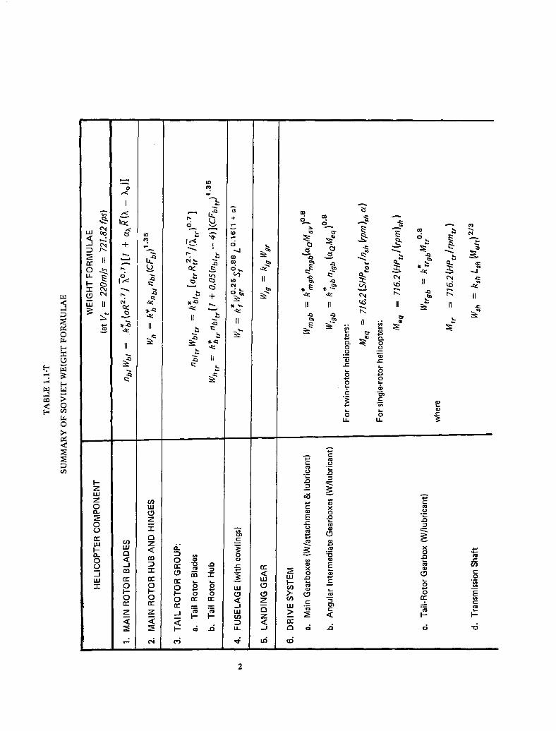


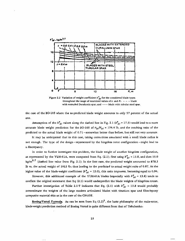

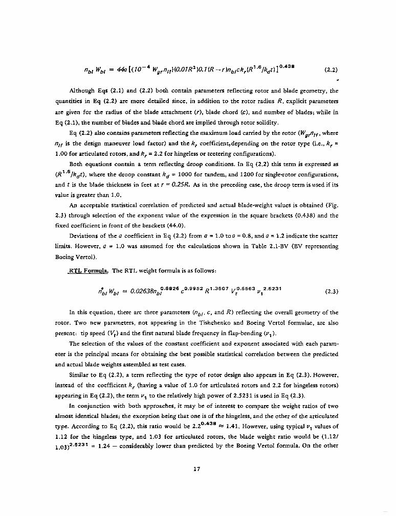


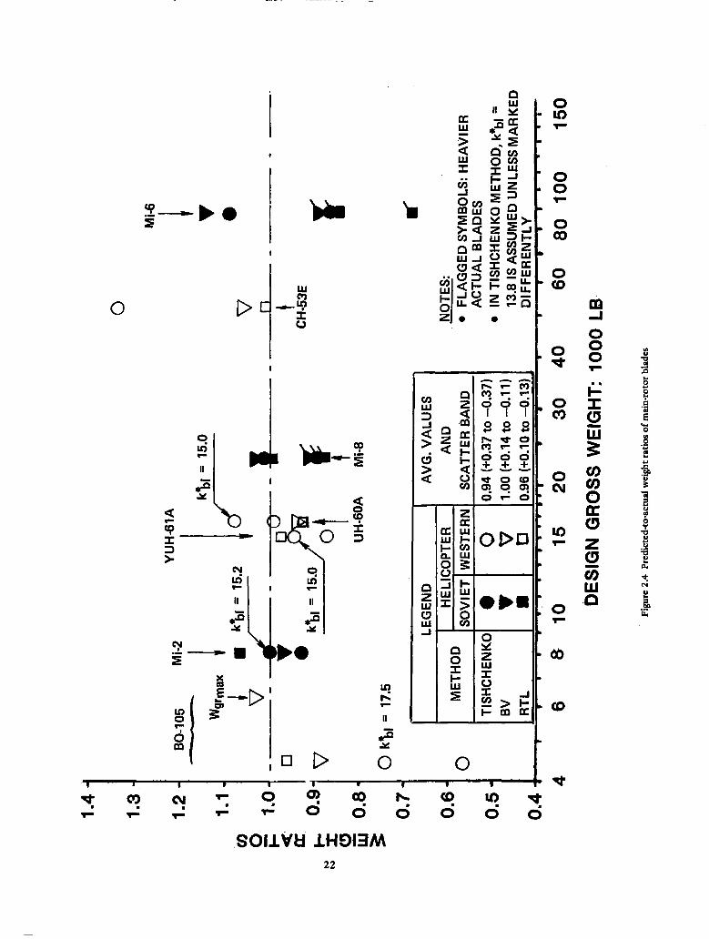

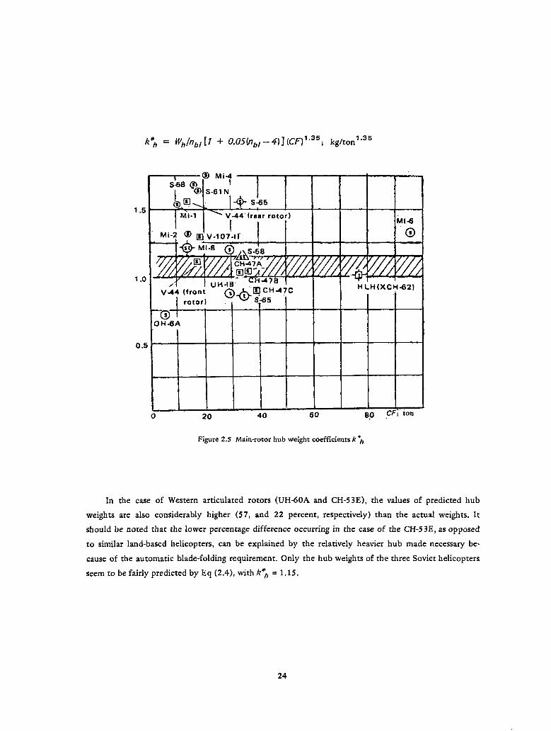


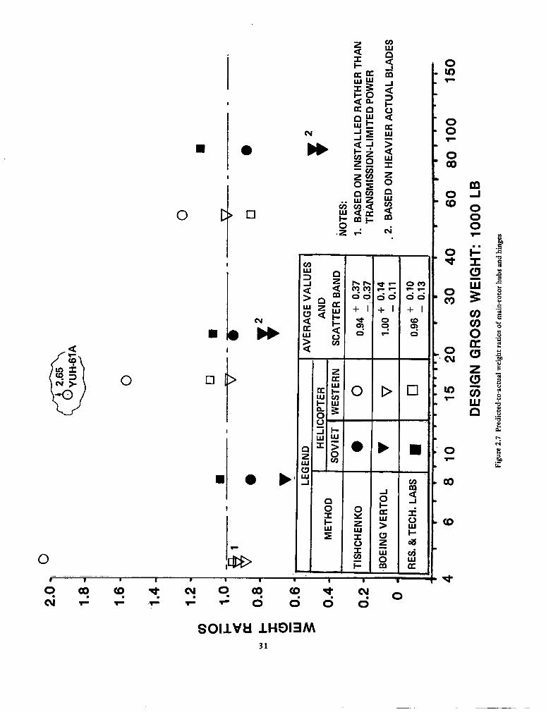


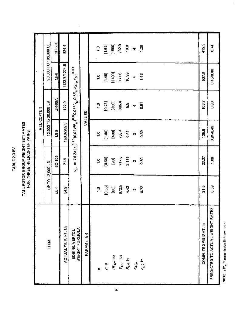


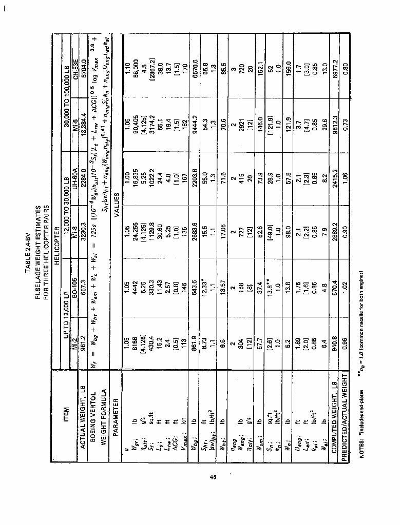


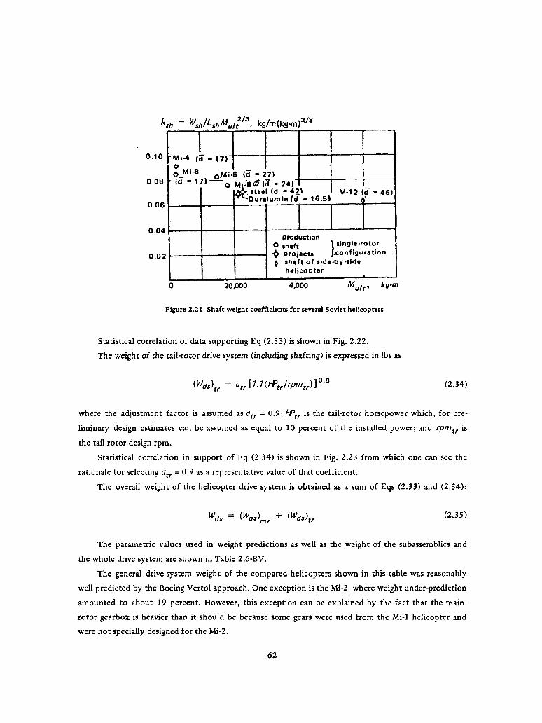


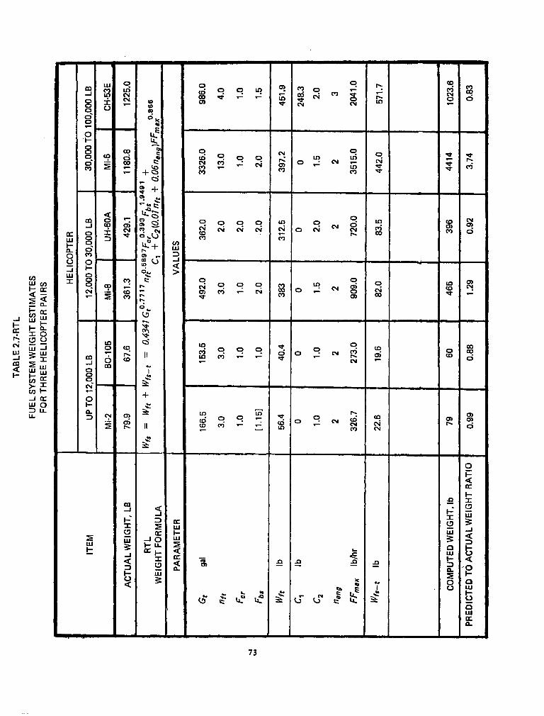


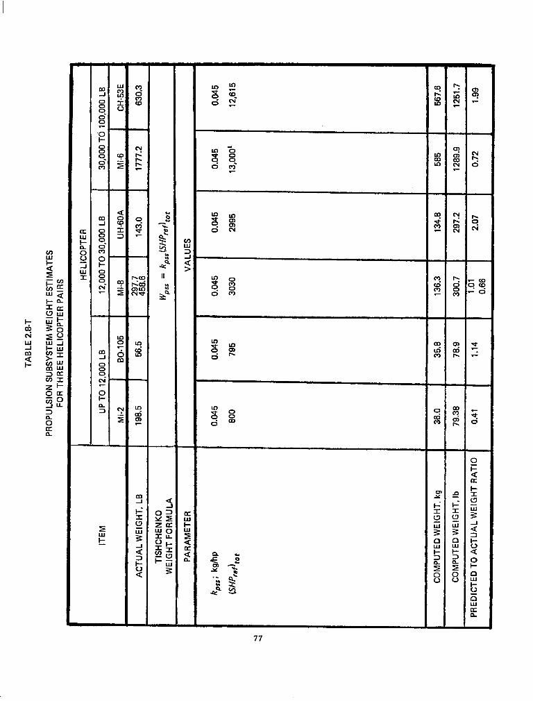


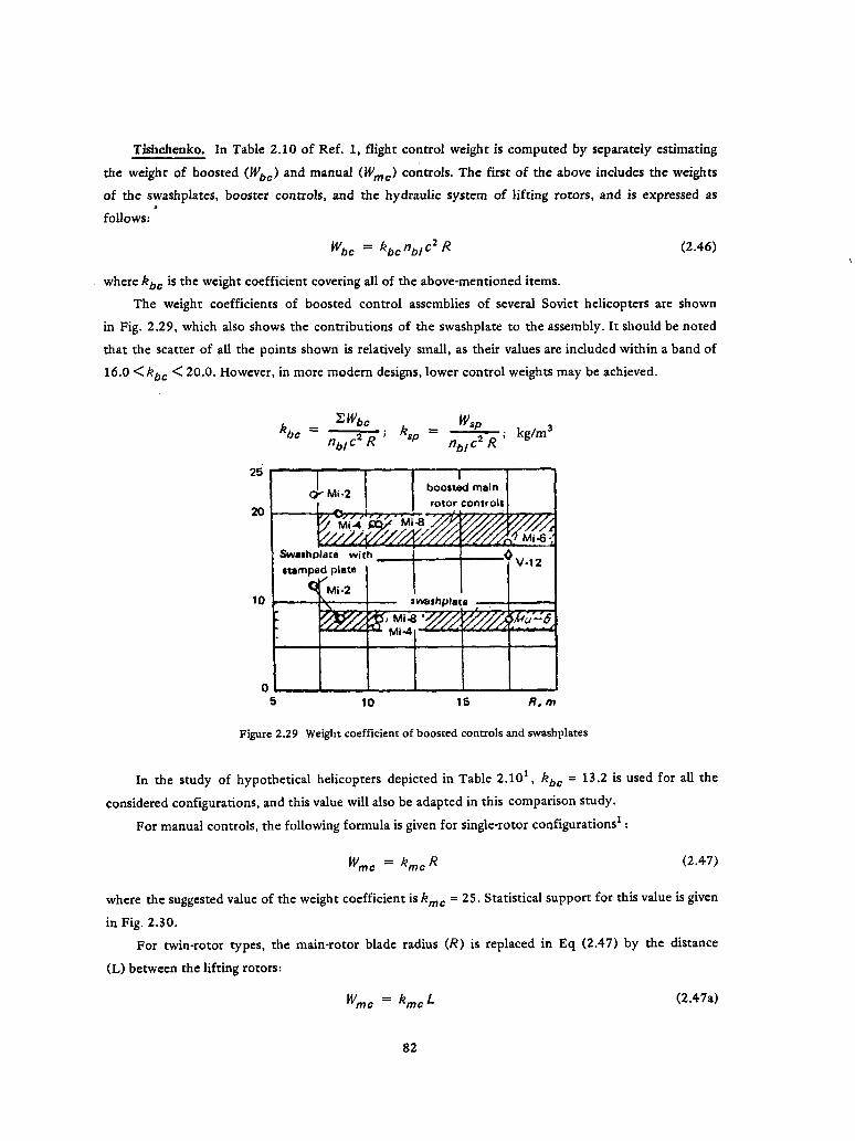


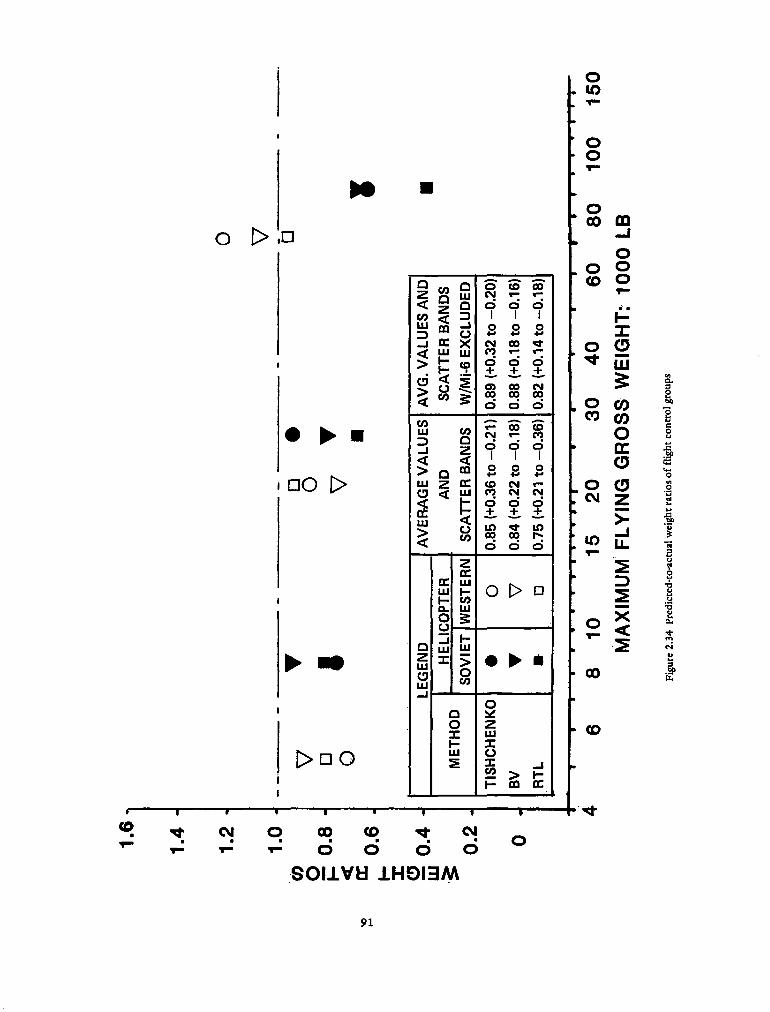


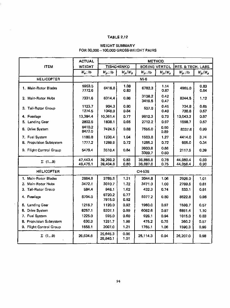


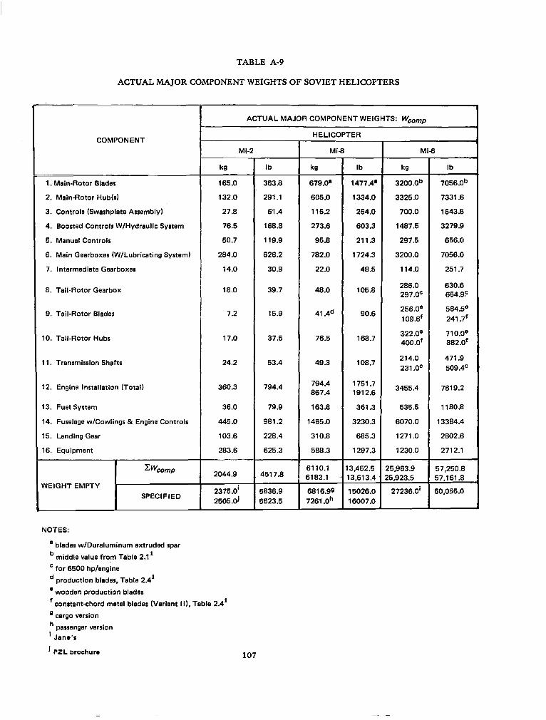


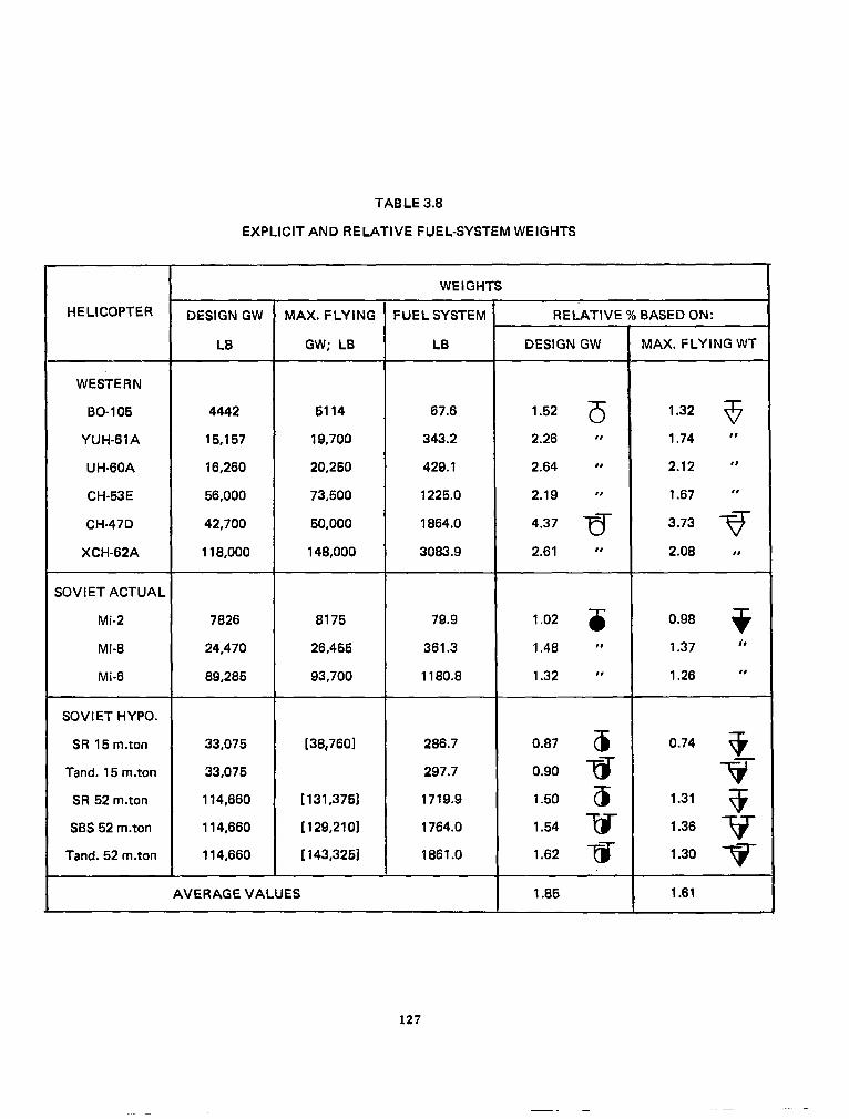


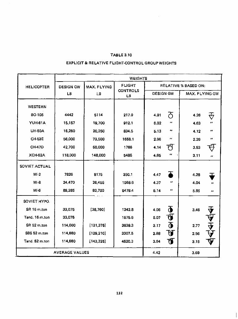


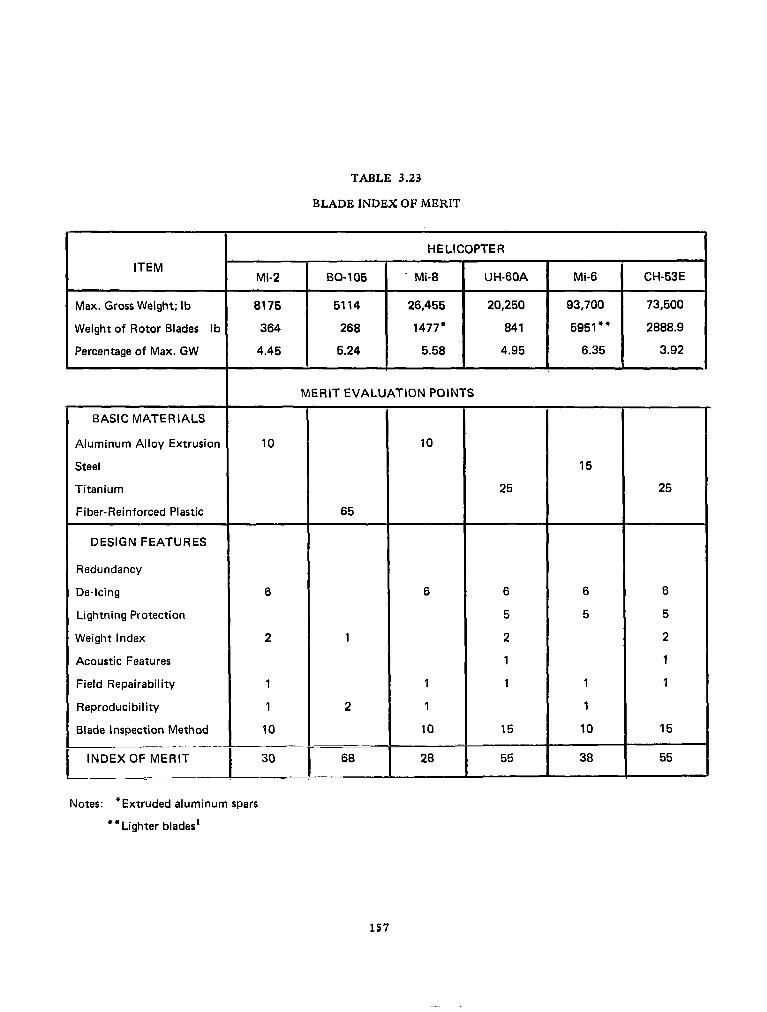


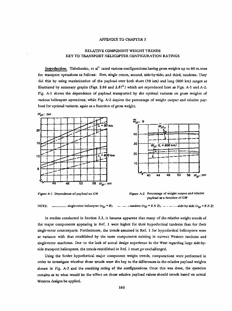


![, NASA Contractor Report ]72 8](https://static.documents.pub/doc/80x56/61f5f30f5bdb351c3b2be492/-nasa-contractor-report-72-8.jpg)


