NASA Contractor Report ICASE Report No. 93-25 191471 /H- y /7 7o IC S 2O Years of Excellence FINITE DIFFERENCE SCHEMES FOR LONG-TIME INTEGRATION Zigo Haras Shlomo Ta'asan NASA Contract Nos. NAS 1-19480, NAS 1-18605 June 1993 Institute for Computer Applications in Science and Engineering NASA Langley Research Center Hampton, Virginia 23681-0001 Operated by the Universities Space Research Association National Aeronautics and Space Administration Langley Research Center Hampton, Virginia 23681-0001 N ,4" ,_ 0 O _n P.. ,4" U r,- Z _ 0 w ZZ wO w;.- OW luZ_ ZW_ b-4_ w _0 -,t-J ,'_00 I w Z _ ._- | xj https://ntrs.nasa.gov/search.jsp?R=19940006187 2018-11-11T19:34:43+00:00Z
Transcript
NASA Contractor Report
ICASE Report No. 93-25
191471
/H- y/7 7o
IC S 2OYears of
Excellence
FINITE DIFFERENCE SCHEMES FOR
LONG-TIME INTEGRATION
Zigo Haras
Shlomo Ta'asan
NASA Contract Nos. NAS 1-19480, NAS 1-18605
June 1993
Institute for Computer Applications in Science and Engineering
NASA Langley Research Center
Hampton, Virginia 23681-0001
Operated by the Universities Space Research Association
National Aeronautics and
Space Administration
Langley Research CenterHampton, Virginia 23681-0001
Finite difference schemes for long-time integration
Zigo Haras and Shlomo Ta'asan *
Department of Applied Mathematics and Computer Science
The Weizmann Institute of Science
and
Institute for Computer Applications in Science and Engineering
Abstract
Finite difference schemes for the evaluation of first and second derivatives are presented.
These second order compact schemes were designed for long-time integration of evolution equa-tions by solving a quadratic constrained minimization problem. The quadratic cost function
measures the global truncation error while taking into account the initial data. The resulting
schemes are applicable for integration times fourfold, or more, longer than similar previously
studied schemes. A similar approach was used to Obtain improved integration schemes.
*This research was made possible in part by funds granted to the second author through a fellowship programsponsored by the Charles H. Revson Foundation and in part by the National Aeronautics and Space Administrationunder NASA Contract No. NAS1-19480 and NAS1-18605 while the authors were in residence at ICASE, NASA
Langley Research Center, Hampton, Va 23681
1 Introduction
The simulation of hyperbolic partial differential equations often requires long-time integration.
The physical phenomena described by these equations typically possess a range of space and time
scales, turbulent fluid flow is a common example. Accurate numerical simulation of this type o_
processes requires proper representation of all the relevant physical scales in the numerical model.
These requirements lead recently to new interest in Pade approximations also known as compact
finite difference schemes [7].
Compact finite difference schemes had long been known and used in numerical analysis [1, 2, 3].
They offer a means of obtaining high order approximations to differential operators using narrow
stencils. This is achieved by treating the sought derivatives as unknowns and solving a system of
equations for them. Typically, the resulting matrices are tridiagonal or pentadiagonal, which can
be efficiently solved .
In [7] a class of highly accurate compact schemes for first, second and higher derivatives were
presented and analyzed. A notion of resolving ej_iciency was introduced which should measure
the accuracy with which the finite difference approximation represents the exact solution over
the full range of length scales that can be realized on a given grid. This criterion was then used
to compare various schemes and motivated the design of a new class of schemes, the so-called
schemes with spectral like resolution. These are fourth order pentadiagonal systems with seven
points stencils. Their improved resolution characteristics were obtained by giving up on high
formal accuracy; instead, requiring that the symbol of the discrete difference operator should
agree with the differential operator at three prescribed high frequencies. However, the resolving
efficiency is a too crude measure as it assumes that all frequencies occur with similar magnitude in
the initial data. In the present paper it is shown that for problems with various initial conditions
these schemes are far from optimal.
A different measure for evaluating finite difference schemes is the L2 norm of the local trunca-
tion error. This measure which takes into account the Fourier components present in the solution
and their amplitude was applied in [9] to design explicit time marching schemes (i.e., discretiz-
ing time and space simultaneously) by solving analytically constrained minimization problems
with quadratic cost. This error measure seems more adequate for comparing difference schemes.
However, the simultaneous treatment of time and space results in very complex optimization
problems. The generalization of the approach of [9] to problems in higher dimensions requires
solving nonlinear constrained optimization over a large set of parameters. It is also hard to apply
that approach to compact schemes. This complexity and the use of analytic rather than numerical
methods makes the suggested approach impractical.
In [4] a heuristic derivation was done by minimizing the weighted error (in the Fourier space)
of the discrete and continuous operators.
The present paper uses the same cost function as [9] with several important differences. First,
improved bounds on the truncation error weie derived. These enabled us to treat time and
space discretizations separately. This greatly simplifies the minimization problem by reducing
it to two lower dimensional problems. Further simplification is obtained by optimizing each
partial derivative separately, instead of approximating the whole differential operator as was done
in [9]. These reductions of problem complexity resulted in a simple and general approach to
synthesis of discretization schemes. It enabled us to design highly accurate compact difference
schemes and integration formulas for various operators and initial data. The resulting second
orderapproximationsprovedto be robust to perturbationsin the spectrumof the initial data,exhibiting .,resolution superior to other known schemes.
The organization of the paper is as follows. In Section 2 Fourier analysis is used to obtain
bounds on the truncation error. In section 3 approximations to derivatives are presented, for the
first and second derivatives and first derivative at mid cell points. Appendices A-C list coefficients
for these derivatives for various stencils and initial conditions. Improved time integration schemes
are developed in section 4, and their coefficients are listed at Appendix D. Section 5 discusses
generalization of the present approach to more complex problems. Numerical results are presented
in section 6. Concluding remarks are made in section 7.
2 Bounds on the truncation error
The application of Fourier analysis for the design and evaluation of finite difference schemes can
be found in many sources, e.g., [9, 10]. In [12] the use of Fourier analysis in the numerical
approximation of hyperbolic problems is extensively discussed.
In the following section bounds on the L2 norm of the error in the discrete solution are derived,
accounting for the effect of discretization both in space and time. These estimates are used in
subsequent sections to design highly accurate schemes.Consider a linear constant coefficient partial differential equation with periodic boundary
conditions of the form :
cOu = Lu (2.1)0t
u(x,o) = uo(x) (2.2)
Further assume that the solution of equation (2.2) does not grow in time.
The discrete analog of this equation can be written as :
u_ +' = P(h, At)u_ (2.3)
u_, = uo (2.4)
where h is the meshsize in space, and P(h, At) is a stable finite difference approximation.
We would like to bound the L2 norm of the error in the discrete solution, for the initial value
A constrained minimization problem of the same type as in the previous sections was formulated
and solved for these symbols.
4 • Approximation of the integration operator
The design of integration schemes is substantially limited by the stability requirement which
renders high order schemes computationally costly. It is well known [5] that an explicit k th order
Runge-Kutta method, with k > 4, should employ at least k+ 1 stages or function evaluations. This
large number of function evaluations makes high order schemes impractical. Therefore, effortshave been made to obtain schemes of lower order with improved characteristics. Within this
approach, the free variables in the Runge-Kutta schemes were set to yield better truncation error
[5] or extended stability region [6]. A generalization of this idea is to give up on formal accuracy
in order to obtain better approximation of the wavenumbers relevant to the problem solved.
The discrete time integration of linear constant coefficient partial differential equation
_U
O--i= Lu (4.1)
amounts to approximation of the exact discrete solution eLhtuo. Therefore, the integration scheme
may be written as?%
p,_(LhAt) = _ai(LhAt) i (4.2)i----O
where ai may depend on L h. The order of the integration scheme is determined by the number
of first terms ai which agrees with the Taylor expansion of e_.
The derivation of the integration schemes is similar to that of derivative discretization, i.e.,
a constrained quadratic optimization problem is formulated based on the error estimate (2.20).
The solution of this minimization problem yields an improved integration scheme. However, the
derivation of integration schemes is more involved than the generation of compact schemes since
the stability condition leads to a nonllnearly constrained minimization problem.
where L h is the discrete approximation of L and p is the order of the n stage formula. Condition
(4.4) can be treated by substitution, but the stability condition requires an explicit treatment.
In accordance with our general approach, we believe that second order formal accuracy suffices.
It remains to determine the number of stages in the integration formula. This should be chosen
to assure that the error in space and time discretizations (2.14) and (2.20), respectively, will be
of similar magnitude. In the present work five stage schemes of second order were investigated,
i.e., n = 5 and p = 2. Integration formulas were obtained for optimized seven point tridiagonal
compact schemes approximating the first derivative, and were tested for the advection equation
in one and two space dimensions.
An important feature of the present approach is that once a feasible minimum has been found
for a prescribed initial value and a given CFL number, the generated scheme will be stable for
this data. This might enable the use of somewhat larger time steps.
5 Approximation of differential operators
The method introduced in the previous sections for generating optimal finite difference approxi-
mations for derivatives and time integration schemes for linear constant coefficient equations can
be extended to more general equations. These ideas can be easily adapted to handle with similar
efficiency more involved problems.The error bounds derived in Section 2 can be generalized for d dimensional problems; noting
that the same proof holds for the d dimensional case after changing the integration over [-_, _]
to multi integration over the box [__,_]d. This suggests that approximation of the differen-
tial equation should be obtained by solving constrained optimization problems in d dimensional
Fourier space for a large set of parameters. For some equations, solving this large minimization
problem might be essential to achieve accurate schemes. Quite often, though, a set of simpler
minimization problems can be obtained by optimizing each partial derivative separately, resulting
in highly accurate approximations.
The approach, which was successfully tested in the present paper, divides the optimization
process into two stages. In the first stage a set of schemes are designed for a large enough
variety of typical initial data (e.g., Gaussians with different parameters, in our examples). This
precomputation is performed once and its results are used in subsequent simulations. In the
second stage, the actual simulation, the initial data uo is Fourier transformed to obtain _o.
The discretization of the partial derivatives is determined by approximating fie as a product of
one dimensional functions for which optimized schemes wore (losigne(I. Eac'h partial derivative
is discretizedusingthe correspondingonedimensionaloptimized scheme. The time marching
scheme is selected from the set of scheme corresponding to the approximating one dimensional
functions. In the present work the selection was done by computing the L2 error norm of each
candidate integration scheme when applied to the approximate initial data with the already
determined discretizations, and selecting the minimum norm scheme. This computation, too, can
be done prior to the actual simulation for a large set of approximated initial data. Thus, the
marching scheme selection can be done by looking up in a precomputed table. The robustness of
the proposed schemes to perturbations in the initial data yields this optimization very efficient;
as can be seen in the numerical results presented in Section 6. It should be noted that the
time required to obtain an appropriate scheme using this approach is negligible relative to thesimulation time.
When the frequencies present in the solution change with time, e.g., due to time dependent
source term, the computation of the optimized schemes should be repeated once a large cumulative
change has occurred. Still,.the relative cost of of this computation is minimal.
The Fourier transform gives the energy content of the whole initial data. It may occur, that
the initial data is smooth at some regions of the computational domain and oscillatory in others,
in which case the designed approximation will give good performances over the whole domain.One can do better by computing a different scheme for each region and using a weighted sum
of the resulting schemes near region boundaries. This requires computing the Fourier transform
locally in each region. The localization to a particular region can be achieve by multiplying u0 by
a C °O function with a compact support which encloses the region.
In some cases, systems of equations may be treated in a similar way. Look first at a one
dimensional first order system
ut = Au_ (5.6)
u(x,0) = u0(x)
where A is a p × p symmetric matrix. Let A = p-1AP be a diagonal matrix, and denote v = Pu.
The discretization of the system
vt = Av, (5.7)
v(x,O) = Puo(x)
can be done in an analogous way to the scalar case, except for the time marching scheme which
should be chosen from a set of candidate schemes (as for the multidimensional scalar equations).
Thus, highly accurate discretization of the system (5.6) can be achieved by first discretizing (5.7)
and using the identity u_ = p-1 v_. For systems in higher dimension
fi Ou (5.8)u_ = Ai-_x i
i--'--1
u(x,0) = no(x)
each partial derivative should be optimized separately. In this case, we require that all Ai will be
symmetric, but it is not necessary that they are simultaneously diagonalizable.
The proposed schemes might be useful for nonlinear equations,-as well. There, one should
design the schemes for the linearized equation; and will be obliged modify them once a large
change in the amplitude of the wavenumbers appearing in the solution occur.
6 Numerical results
6.1 Approximation of derivatives
The constrained minimization problem (3.5) for the space discretization can be easily solved by
substitution using (3.2). Differentiation of the resulting quadratic form provides a set of necessary
conditions holding at the minimum. This nonlinear system can be solved using Newton method,
yielding a local minimum. Since the schemes obtained using this process significantly improve
previously known schemes [7], no attempts were made to find the other zeroes of the nonlinear
system, searching for better minima.
Three types of schemes were studied : (a) tridiagonal with five points stencil, i.e., fl = c = 0 ,
(b) tridiagonal with seven points stencil, i.e., fl = 0, (c) pentadiagonal with seven points stencil.
The initial approximation to the Newton iteration was, typically, a compact scheme with the same
structure, taken from [7].
It can be observed, in figures 1 and 5, that the modulos of symbol of the optimized penta-
diagonal scheme for the first and second derivative is larger then the modulus of the differential
symbol. This error is exceedingly larger for schemes generated to approximate narrower spectra.
The overshooting occurs in the highest end of the spectrum for wavenumbers not appearing in
the solution. However, since the stability of a scheme is determined by the values assumed by
Lh(wh) [11], this type of scheme is applicable only with small CFL. Moreover, the desired ro-
bustness is limited by this phenomenon. Therefore, this behavior of the approximation can not
be ignored. A possible remedy can be found in searching for other minimizers of the quadratic
form. Using the tridiagonal scheme as initial approximation for the Newton process converged
to solutions without this limiting property but with reduced resolution, similar to the tridiago-
hal schemes. Other possible directions, e.g., further looking for other minima or penalizing in
the cost function for this behavior were not explored. This is since we believe that for practical
applications pentadiagonal systems are too costly to solve, whereas the tridiagonal schemes offer
similar resolution characteristics, are easier to solve and do not suffer from this deficiency. The
pentadiagonal scheme are given mainly for theoretical reasons as a counterpart to the spectral-like
approximations.
A proper appreciation of the superiority of the proposed schemes can be gained by integrating
with them hyperbolic equations for long time, provided the integration process introduces only
negligible numerical errors. This requirement necessitates either using high order integration
schemes or employing exact integration, as was done in the present work. The experiments
described in next subsections clearly demonstrate the superior behavior of the proposed optimized
schemes.
6.1.1 Approximation of the first derivative
Compact finite difference schemes were designed and tested for initial data of the form e -a_'2 for
several values of _. In Figure 1, the symbols of schemes corresponding to a = 2 are plotted, as
well as the weighted error
]L(wh)- Lh(wh)]l_(wh)[ (6.9)
forthemoreaccurateschemes.Thecoefficientsoftheoptimizedschemescanbefoundin AppendixA. Thecoefficientsof the otherschemesweretakenfrom [7]. Forscheme(a) thecoefficientswere
a = _,_ = 0, a = ,b = _,c = 0 (6.10)
The coefficients of scheme (c) were
25 1 1= 0,a=
The coefficients of the spectral-like scheme (e) were
(6.11)
a = 0.5771439, fl = 0.0896406, a = 1.3025166, b = 0.99355, c = 0.03750245 (6.12)
It can be seen that each optimized scheme better approximates the differential operator than
its non-optimized counterpart. In Figure l, one can observe that although the symbol of the
spectral-like pentadiagonal scheme follows the differential symbol for more wavenumbers than the
tridiagonal scheme, the L2 norm of truncation error of tridiagonal scheme is somewhat smaller
for this data. This can be explained by noting that the error of the tridiagonal scheme is mainly
in the high frequencies while the spectral-like scheme has large error at the smoother Fourier
components where the present initial data has more energy. The spectral-like scheme attains
better resolution at the expense of larger error in lower frequencies. The error in the optimized
schemes is significantly smaller than in their counterparts. More precisely, computing the error
norms reveals that the error in the tridiagonal scheme is about six times larger than in the
optimized tridiagonal scheme while error norm of the spectral-like scheme is about seventeen
times larger than in the optimized pentadlagonal. The plot of the absolute value of the erroralso reveals that the L2 norm was used as a minimization criteria. This can be seen from the
several sign changes of the error of the optimized schemes, being in accordance with the averaging
property of the chosen norm.
Figure 2 demonstrates the better resolution of the optimized scheme by exact integrating in
Fourier space on a 32 points grid with the pentadiagonal spectral-like scheme and the pentadiag-
onal optimized scheme the equationOU OU
_ (6.13)Ot Ox
a = 0.8 (a being the CFL number) was used. It is shown that at time T = 10000, the error in the
solution using the optimized scheme is smaller than the error at time T = 1000 when using the
spectral-like scheme. This suggests that the optimized scheme can be used for integration time
at least ten times longer than the spectral-like scheme, in close accordance with the ratio of the
error norms.
Figure 3 displays the scheme's robustness to perturbation in initial condition. The solution
integrated with the optimized scheme far better approximates the exact solution than the one
employing the spectral-like approximation, even for initial data different from the one it was
designed to resolve. This holds for both smoother and more oscillatory initial data. Although
those examples do not give a quantitative view on the relative efficiency of the schemes for those
initial data, one can see in both figures that by the time the solution with the optimized scheme
developed significant error the error in the one corresponding to the spectral-like scheme is so
large it no longer approximates the exact solution.
10
Figure4 showsatwodimensionalequationwhichdemonstratestherobustnessof theproposedschemes.In this examplethe initial datawastakento be the Gaussiane -(°_+5_) rotated at an
angle of _. Then the program searched for initial data of the form e,(_'l_'_ +n2_]), for the integers
1 < nl,n2 _< 7 which yielded the best approximation to the initial data. The pentadiagonal
schemes optimized for initial data e -'_2 and e -'_2_'_ were then used to compute ux and uv,
respectively. In this example nl = 3 and n2 = 2. The resulting semi discrete system was solved
by exact integration in Fourier space on a 32 x 32 grid. The plot shows a cut through the solution in
the x direction containing the maximum point of the solution. While the solution corresponding
to the optimized disretization closely approximates the exact solution, the solution discretized
with the spectral-like scheme bears very little resemblance to the exact solution.
6.1.2 Approximation of the second derivative
The coefficients of compact schemes for various initial conditions of the form e -a_'2 can be found
in Appendix B.
Figure 5 plots absolute value of the symbol of the second derivative and the weighted error,
for a = 2. The parameters of the optimized schemes can be found in Appendix B. The coefficients
of the other schemes were taken from [7]. Scheme (a) is given by :
The coefficients of the spectral-like pentadiagonal scheme (e) are :
a = 0.50209266,fl = 0.05669169,a = 0.21564935,b = 1.723322, e = 0.1765973 (6.16)
It can be seen that the error in the non optimized schemes is significantly larger than in the
optimized ones. It is interesting to note that, again, for this specific data the L2 error norm of
the spectral-like scheme is about an order of magnitude larger than the non optimized tridiagonal
scheme. This phenomenon suggests that the resolution efficiency is a poor estimate for discretiza-
tions evaluation. Computing the error norms reveals that the error in the optimized tridiagonal
scheme is about seven times smaller than in the non optimized scheme, whereas the error in the
optimized pentadiagonal scheme is seventy times smaller than the spectral-like scheme, for this
given data.
The efficiency of the pentadiagonal schemes was compared by integrating the wave equation :
02 U 02 U_ (6.17)
Or2 Ox 2
This equation was put in a system form :
(0--- 02
v t _
11
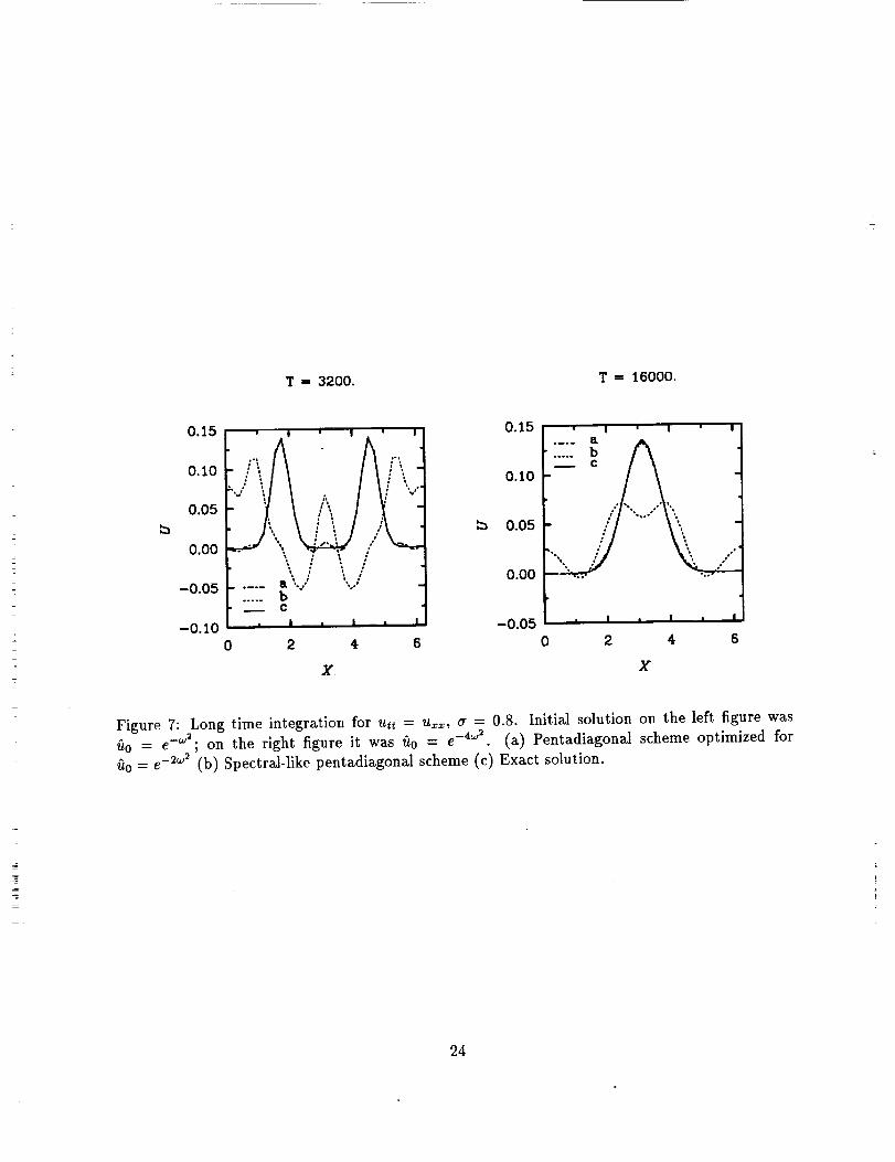
This systemwasexact integratedon a 32points grid and the resultsaregivenin Figures6-7demonstratingthe improvedaccuracyof the optimizedschemeandits robustness,respectively.Figure6 demonstratesthat the optimizedschemecanbeusedfor integrationtime 37 times,ormore,longerthan thespectral-likescheme.In Figure7the schemerobustnessisclearlyshownforinitial datasmootheror moreoscillatorythan thedatafor whichtheschemewasdesigned.In bothcases,by the timea significanterroroccursin the solutiondiscretizedwith theoptimizedschemethe solutioncorrespondingto the spectrallike schemetotally differsfrom theexactsolution.
Theinitial solutionand its approximation,for the twodimensionalproblemin Figure8 wereobtainedsimilarly to thoseof the examplein Figure4. While the solutionintegratedwith theoptimizedschemecloselyapproximatesthe exact solution, it is hard to seethat the solutioncorrespondingto thespectral-likeschemeindeedapproximatesthe sameproblem.
6.1.3 Mid cell approximation of the first derivative
Appendix C lists the coet_cients of schemes designed for various initial data. The coefficients of
the schemes taken from [7] are listed below. Scheme (a) is given by :
a = -_2,_ = O,a = 3 (3- 2ct),b= l (22a-1),c = O (6.19)
The coefficients of scheme (c) are:
75 37950 - 39725a, b 65115a - 3350 25669a - 6114a = _-_, fl = 0, a = = , c = (6.20)31368 20912 62736
The coefficientsofthe tenthorderpentadiagonalscheme (f)are :
The standard compact schemes give very good resolution in this form (see Figure 9), thus,
the improvement introduced by the optimized schemes is smaller. Optimizing the tridiagonal
scheme yields a 6.5 smaller error norm while optimizing the pentadiagonal scheme yields a 2.5
times smaller norm. In this case, the error norm of the optimized tridiagonal scheme is very close
to that of the non optimized pentadiagonal scheme.
An interesting option suggested by this approach was to optimize the _ operator in order tod 2
get the best approximation for _-FJ, for given initial values. This has been done for the tridiagonalscheme which was used to integrate equation (6.17). It was compared, in Figure 10, to the
tridiagonal scheme from [7] where both are used to approximate the second derivative in solving
the one dimensional wave equation in the system form (6.18). Again, the optimized scheme gives
significantly better approximation.
6.2 Approximate time integration
The constrained minimization (4.3)-(4.5) was solved by requiring that the solution will touch
the stability constraint at one point while maintaining global stability and and minimizing the
functional. The point which gives best result was found by exhaustive search. This straightforward
approach yielded the local minima reported in this paper. Somewhat better integration schemes
might be achieved by using more advanced optimization techniques [8].
12
Accordingto the generalapproachoutlined in Section 5, one should choose an integration
scheme which yields truncation error of similar magnitude in time and space. Since the stability
region for several fifth order six stages explicit Runge-Kutta schemes intersects the imaginary
axis only in a small neighborhood of the origin [5, 6] disabling time marching with large CFL, the
optimized scheme was compared with the four stage fourth order Runge-Kutta. We preferred this
five stage scheme which has an error norm about five times larger than the space discretization to
the seventh order scheme which yields an error norm about eleven times smaller than the space
discretization because of its lower computational cost.
The analysis performed in Section 2 suggests that the integration operator should be opti-
mized with respect to the spatial discrete operator employed, i.e., to minimize I[p(Lh(wh)At) -
eLh(wh)atllL2 In the following examples L h is the tridiagonal approximation for _,d when initial
data is e -2W2 and _r = 0.8. Appendix D contains the coefficients of integration schemes for various
initial data when L h is the tridiagonal scheme optimized for the same initial data and a = 0.8.
Figure 11 plots the real and imaginary parts of e Lh(Wh)At versus the four stage fourth order
Runge-Kutta and the improved scheme. The norm of the imaginary part of the error was reduced
by a factor of 31 while its real part was reduced by merely a factor of 2.3.
Figures 12-13 shows the integration of the advection equation with those scheme on a 32 points
grid, demonstrating the superior efficiency and robustness of the proposed schemes. In Figure 12
one can see that the optimized scheme can be used for at least three times longer integration time
than the Runge-Kutta scheme applied to the tridiagonal scheme from [7]. The computed error
norms suggests the time marching error is dominant in all examples.The two dimensional example in Figure 14 summarizes the approach suggested in this work.
It compares the optimized tridiagonal scheme combined with the appropriate integration formula,
to fourth order Runge Kutta applied to non-optimized tridiagonal discretization. Although the
analysis in Section 2 applies only to constant coefficient problems, this example shows it holds,
heuristicly, to variable coefficient equations, as well. The initial data for this problem was obtained
in a similar manner to that in example 4. However, instead of comparing the solutions computed
on the 32 x 32 grid to the exact solution, they are compared to the solution on a 64 x 64 grid
which was integrated with the optimized scheme designed for the narrowest computed Gaussian
(a = 7). The initial data for the finer grid was obtained by bilinear interpolation from the coarser
grid. It can be seen that the optimized scheme yields significantly more accurate solution.
7 Conclusion
A simple and general approach for the design of finite difference approximation of derivatives
and integration formulas was introduced. It was used to design compact finite difference schemes
for derivatives evaluation; and the resulting schemes were compared to previously known similar
schemes. The guiding line has been to improve the representation of the range of wavenumbers
appearing in the physical problem being solved, taking into account their relative amplitudes.
This lead to an L2 measure of the approximation. The resulting schemes combined adaptivity to
the specific initial data by the nature of their design and robustness to perturbations in the initial
data. The improved resolution had been demonstrated for several problems.
A similar approach was used to design improved integration schemes, taking into account the
spatial discretization as well as the initial data.
Figure 3: Long time integration of the equation ut = u_:, cr = 0.8. Initial solution on the left--022figure was Uo e ; on the right figure it was u0 = e -4°J2.
(a) Pentadiagonal scheme optimized for _20 = e -:_2 (b) Spectral-like pentadiagonal scheme (c)
Exact solution.
21
T = 6500.
0.04
0.03
0.02
0.01
0.00
-0o01
| | | |
! i e I
C
0 2 4 6
X
Figure 4: Integration of the equation u, = ux + uu, cr = 0.8 using pentadiagonal schemes. Initial
solution was rio e-(_+sw_ ) rotated at an angle of _ This data was approximated by unrotated-- _.
Figure 8: Long time integration for utt = u** + uuu, a = 0.8 using pentadiagonal schemes.
'_ This dataInitial solution on the left figure was fi0 = e -(_+s_]) rotated at an angle of 7"
was approximated by unrotated gaussian e-(3_+2_] }. (a) Optimized pentadiagonal scheme (b)
Spectral-like pentadiagonal (c) Exact solution.
25
3.00
2.00
1.00
0.00
0
w | w
.... b
.-_C f
m I m
2
_a_enwrnber-_
Figure 9: Symbol for mid-ceU discretizations of _, % = e -2_2. (a) Sixth order tridiagonal
scheme (/3 = c = 0) (b) Second order optimized tridiagonal scheme (t3 = c = 0) (c) Eighth order
tridiagonal scheme (/3 = 0) (d) Second order optimized tridiag0nal scheme (/3 = 0) (e) Tenth
order pentadiagonal (f) Optimized pentadiagonal. (g) Exact symbol. Schemes were optimized for
UO ---- e-2W2-
1!
J
i
i|
!I
26
T - 4500.
L ' I ' I ' I1
0.10 / ,'5 /': :':, /_ /
[/i:':'/11/ - / '../ '.. : '.,
0.05 / ", : ': -,. ,,I IV# t
0.00 ...."" "--
b
m C
, I , I , i-0.05
0 2 4 6
X
Figure 10: Long time integration for utt = uxz, _t0 = e -2w2 o" = 0.8. (a) Non optimized tridiagonald2
scheme (b) Tridiagonal mid-ceU discretization scheme of d optimized to approximate _ when
rio = e-2_' (c) Exact solution.
27
1.00 1.0 . i '
0.80
(0.60 ( 0.5_ 0.400.2.0 0.0
0.00
-0.20 -0.50 2 0 2
Figure 11: Real and imaginary parts of approximations to eLh(w), where Lh(_) is the symbol
of the tridiagonal scheme for _ optimized for u0 = e-2_2 and a = 0.8. (a) Five stage scheme
optimized for the same a (b) Fourth order Runge-Kutta (c) Exact time integration.
T - 150• T " 450.
0.20
0.15
0.10
0.05
0.00
-0.05
' I ' I ' II
• .... 'b
_..r m. •
• I • • • I
0 2 4 6
0.20
0.15
0.10
0.05
0.00
-0.050
' I ' j%l ' I=_.. i A
iB*e %1 _' w
\ /I1o _ =
,,1 ! i I , I
2 4 6
X X
Figure 12: Integration of ut = u=, _o = e -2_'2, a = 0.8. The space derivative is computed using
the tridiagonal compact scheme optimized for the same initial date and a. (a) Five stage scheme
optimized for this scheme and CFL (b) Fourth order Runge Kutta (c) Exact time integration
28
T= 45. T = 1000.
0.30
0.20
0.10
0.00
-0.I0
0 2 4 6
0.15
0.10
0.05
0,00
• I ' I ' I
-0.05 ' ' ' ' ' '
0 2 4 6
X X
--oj 2Figure 13: Integration of ut = u,, a = 0.8. Left: rio = e ; Right: rio = e-4_2. (a) Five
stage scheme optimized for this scheme and CFL (b) Fourth order Runge Kutta (c) Exact time
integration.
29
T = 400.
0.04 [ , | , , , ,_
0.03
0.02
0.01
0.00
C
-0.010 2 4 6
X
Figure 14: Integration of ut = u= + 0.5(1 + 0.6sin(2ry))uy, a = 0.8 using tridiagonal schemes.
Initial solution was rio e-(_+5_ ) rotated at an angle of _ This data was approximated_'.
by unrotated gaussian e -(3_+2_]). (a) Optimized tridiagonal scheme and optimized marching
scheme (b) Tridiagonal scheme integrated with fourth order Runge-Kutta. (c) A fine grid solution
(practically exact)
30
- Form ApprovedREPORT DOCUMENTATION PAGE OMe_o o7o4olea
PuOh< re_rtang burden for this collection of _nformat_oo _s ?st_ateo _,o average _ hour oer _Donse. _nciuding the t_me for revdew_ng instructions, _earc_ng ex,stlng _ata SOurce%
gathering and ma nta_nlng the data needed, and comoletang and reviewing the c311ec_ on of _nformatlon Seno comments re<)arci,ng thgs burden estimate Or any 3tl_er asDe_ of th=_collection of information. _nc_uding $ugge_tion_ for reducing thl_ burcien to V'_/ashmcJton Headouarl"er$ _ervlces. Direc_orate Tot Into ma_ on O¢,eratioi',s and Re_r%, 2 5 _e_erf, on
Dav=s Highway, C_u_te 1204. Arlington. V_, 22202-4302, and to the Office of Management and 8uclget. Paperwork Reduct*on Pro ec_ (0704-018B). Washington. DC 20503
1. AGENCY USE ONLY (Leave blank) 2. REPORTDATE 3, REPORTTYPE AND DATES COVEREDJune 1993 Contractor Report
4. TITLE AND SUBTITLEFINITE DIFFERENCE SCHEMES FOR LONG-TIME INTEGRATION
6. AUTHOR(S)
Zigo HarasShlomo Ta'asan
7. PERFORMINGORGANIZATION NAME(S}AND ADDRESS(ES)
Institute for Computer Applications in Science
and Engineering
Hail Stop 132C, NASA Langley Research Center
Hampton, VA 23681-0001
g. SPONSORING/MONITORING AGENCY NAME(S) AND ADDRESS(ES)