Page 1
NASA
0
i
Z
CONTRACTOR
REPORT
NASA
cO
CR-2470
IMPROVED CURVE FITS FOR THE THERMODYNAMIC
PROPERTIES OF EQUILIBRIUM AIR SUITABLE
FOR NUMERICAL COMPUTATION USING
TIME-DEPENDENT OR SHOCK-CAPTURING METHODS
by J. c. Tannehill and P. H. Mugge
Prepared by
IOWA STATE UNIVERSITY
Ames, Iowa 50010
/or
NATIONAL AERONAUTICSAND SPACE ADMINISTRATION • WASHINGTON, D. C. • OCTOBER 1974
https://ntrs.nasa.gov/search.jsp?R=19740026586 2018-06-27T03:10:53+00:00Z
Page 2
==
T
±i
L_
;_±:!-
== =
Page 3
1. Report No. 2. Government Accession No. 3. Recipient's Catalog No.
NASA CR 21)70
" 4. Title and Subtitle 5. Report Date
OCTOBER 1974"Improved Curve Fits for the Thermodynamic Properties of
Equilibrium Air Suitable for Numerical Computation Using
Time-Dependent or Shock-Capturing Methods"
7, Author(s)
J. C, Tannehill and P.H. _gge
9. Performing Organization Nameand Address
Engineering Research Institute
Iowa State University
Ames, Iowa 50010
12. Sponsoring Agency Name and Address
National Aeronautics & Space Administration
Washington, D.C. 20546
6. Performing Organization Code
8. Performing Organization Report No.
10. Work Unit No.
11. Contract or Grant No,
NGR 16-002-038
13. Type of Report and Period Covered
NASA/Grant, Final Rept, Part 1
14. Sponsoring Agency Code
15. Supplementary Notes
16, Abstract
Simplified curve fits for the thermodynamic properties of equilibrium air have been devised for
use in either the "time-dependent" or "shock-capturing" computational methods. For the
"time-dependent" method, curve fits were developed for p = p{e, p), a = a(e, p), and T = T(e, p),
while for the "shock-capturing" method, curve fits were developed for h = h(p, p) and
T = T{p, p). The ranges of validity for these curve fits are for temperatures up to 25,000 °K and
densities from 10 -7 to 103 amagats. These approximate curve fits may be particularly useful when
employed on advanced computers such as the Burroughs ILLIAC IV or the CDC STAR since they avoid a
cumbersome table-lookup.
7. Key Words (Sugg_ted by Author(s))
Thermodynamic properties,
Equilibrium Air
Real Gas properties
18. Distribution Statement
UNCLASSIFIED-UNLIMITED
19. Security Classif.(ofthisreport)
UNCLASSIFIED
20, SecurityClassif.(ofthis _ge) 21. No. of Pages
UNCLASSIFIED 33
*For sale by the National Technical Information Service, Springfield, Virginia 22151
CAT. 12
22. Price"
$3,25
Page 5
TABLE OF CONTENTS
Summary
Notation
Introduction
Construction of Curve Fits
Equations of Curve Fits
Comparisons with RGAS program
References
Appendix A:
Appendix B:
Appendix C:
Appendix D:
Coefficients for curve fits
Subroutine TGAS for p = p(e, p), a = a(e, 0),
and T = T(e, p)
Subroutine TGAS for h = h(p, p)
Subroutine TGAS for T = T(p, 0)
Page
ii
iii
I
2
5
8
17
19
23
29
32
Page 7
ii
SUMMARY
Simplified curve fits for the thermodynamicproperties of equilibrium
air havebeendevised for use in either the "time-dependent"or "shock-
capturing" computationalmethods. Theaccuracies of these curve fits
are substantially improvedover the accuraciesof previous curve fits
appearingin NASACR-2134. For the "time-dependent"method,curve fits
were developedfor p = p(e, p), a = a(e, p), andT = T(e, p), while for
the "shock-capturing" method,curve fits weredevelopedfor h = h(p, p)
andT = T(p, p). Therangesof validity for these curve fits are the
sameas the NASA-ARCRGASprogram,namely, temperaturesup to 25,000OK
anddensities from 10-7 to 103amagats. Theseapproximatecurve fits
maybe particularly useful whenemployedon advancedcomputerssuchas
the Burrough's ILLIACIV or the CDCSTARsince they avoid the cumbersome
table-lookup feature of the RGASprogram.
Page 8
iii
a = speedof sound
e = internal energy
h = enthalpy
p = pressure
R = gas constant
T = temperature
= h/e
D= density
Subscript
o = standard conditions
NOTATION
Page 9
INTRODUCTION
Whencomputingreal gas flows using a finite-difference solution
of the conservative form of the unsteadyNavier-Stokesequations, it
becomesnecessaryto determinepressure as a function of density (_)i
and internal energy (e). This requirement led to the previous study
in which two different approachesweredevelopedfor the caseof2
equilibrium air. In the first approach, the NASA-AmesRGASprogram
wasmodified to allow density and internal energy to be the independent
variables. This approachpermits a very accurate determination of the
thermodynamicproperties of air. Unfortunately, the table-lookup
feature of the RGASprogramis too cumbersometo be effectively employed
on advancedcomputerssuchas the Burrough's ILLIACIV or the CDCSTAR.
For this reason, and also to reducecomputationtime on conventional
serial computers,simpler approximatemethodswere investigated in the
secondapproach.
In the secondapproach,simplified curve fits were devised for
p = p(e, p), a =a(e, p), andT = T(e, p). In addition, a simplified
curve fit wasmadefor h = h(p, $). This latter curve fit is required
in the "shock-capturing" method3. The rangesof validity for these corre-
lation formulaswere the sameas the RGASsubroutine, namely, temperatures
up to 25,000OKand densities from 10-7 to l03 amagats. Theaccuracies
of these simplified curve fits were muchbetter than the previous curve
fits of Barnwell4, but they did not approachthe accuracyof the modified
RGASprogram. For this reason, the present study wasundertakento sub-
stantially improvethe accuraciesof the previous curve fits without
increasing the required computertime.
Page 10
CONSTRUCTIONOFCURVEFITS
The curve fits wereconstructed using Grabau-typetransition func-
tions5 in a mannersimilar to Lewisand Burgess6 andBarnwell4. A
transition function of this type canbe usedto smoothlyconnect two
surfaces fl(x, y) and f2(x, y). For y = constant, the Grabau-type
transition function (with an inflection point) becomes
f2(x) fl(x)
z = fl(x) + 1 + exp [K(x - Xo)] (I)
where K is the parameter which determines the rate at which z changes
from fl(x) to f2(x), and Xo is the location of the inflection point
as shown in Fig. I.
F2(X, Y)z
I
NSTA NT
FI(×"Y) i
x xo
Fig. i. Grabau-type transition with
inflection point.
In the previous study I, the curve fits were constructed by joining
two Grabau-type transition functions with the equation for a perfect gas.
In the present study, a substantial improvement in accuracy was achieved
by joining together as many as five Grabau-type transition functions with
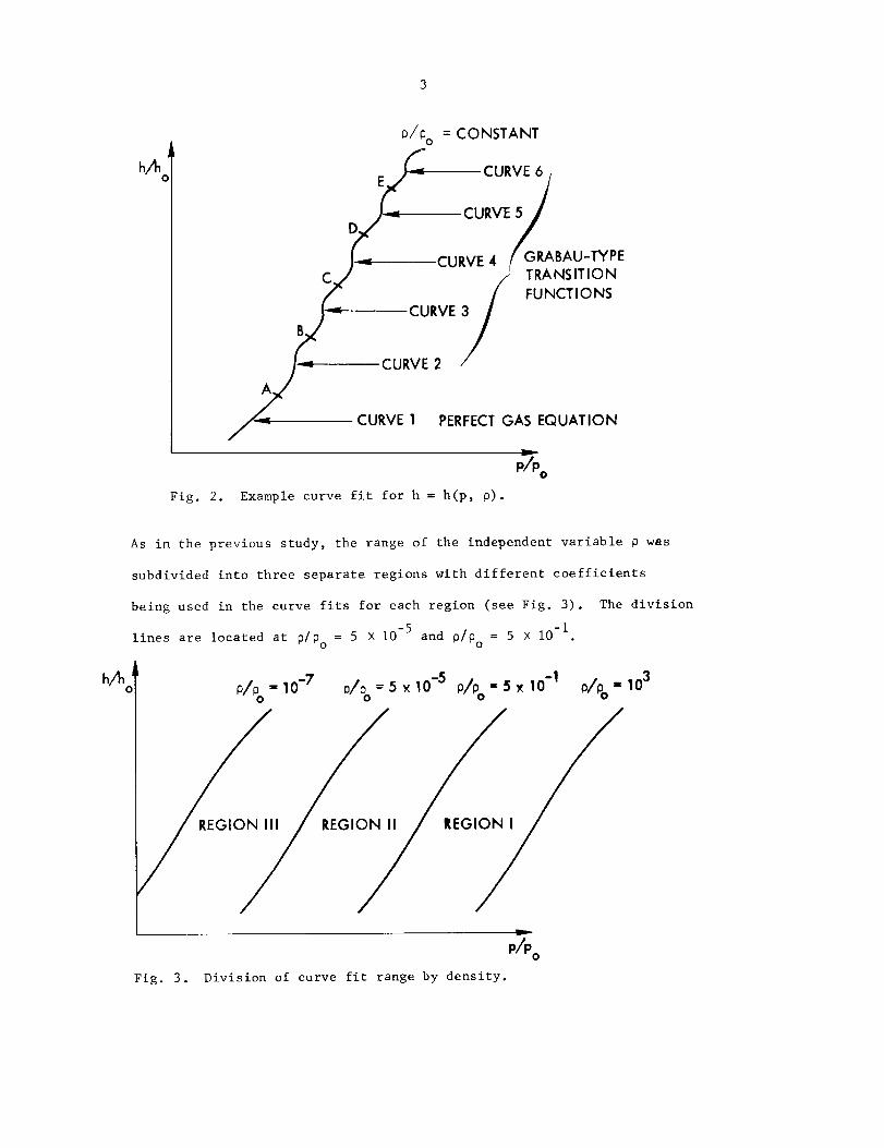
the perfect gas equation as shown in Fig. 2.
Page 11
h/_
Fig. 2.
P/Po = CONSTANT
E _ CURVE 6
I= CURVE4 f GRABAU-n'PE
VE 2
CURVE 1 PERFECTGAS EQUATION
P_PO
Example curve fit for h = h(p, p).
As in the previous study, the range of the independent variable p was
subdivided into three separate regions with different coefficients
being used in the curve fits for each region (see Fig. 3). The division
lines are located at P/Po = 5 X 10 -5 and P/Po = 5 X I0 -I.
h/ j P/Po"1°-7 pl_o: s _ lo-2 _/po,. s x lo-1 _/_o'- lo3
Fig. 3. Division of curve fit range by density.
Page 12
4
The coefficients in the equations for fl(x, y) and f2(x, y) were
determined using a least squares computer program to fit the data from
the original NASA RGAS program. The selection of the form of the equations
for fl(x, y) and f2(x, y) was largely a trial-and-error process. By in-
cluding more terms, a better curve fit was achieved. In fact, if a suffi-
cient number of terms were retained in fl(x, y) and f2(x, y), the accuracy
of these curve fits could be made to approach that of the RGAS program,
but with little savings in computer time.
Page 13
EQUATIONS OF CURVE FITS
p = p(e, p)
For the correlation of p = p(e, p), the ratio _ = h/e was curve-
fitted as a function of e and p so that p can be calculated from
p = pe(_- i) (2)
The general form of the equation used for _ was
_= a + a2Y + a3Z + a4YZ + a5Y2 + a6Z2 + a7YZ2 + a8Z3
a 9 + al0Y + allZ + aI2YZ
+ 1 + exp [(a13 + alAY)(Z + al5Y + a16)] (3)
where Y = Iogi0(0/1.292) and Z = lOglO(e/78408.4). The units for p
m 3 2 sec 2are kg/ and the units for e are m / . The coefficients al, a2, ...,
a16 are given in Table AI, Appendix A, for the entire range of e and p.
It should be noted that many of the terms appearing in Eq. (3) are not
used over the entire range of e and p.
a = a(e, p)
An exact expression for the speed of sound in terms of _ was derived
by Barnwell 4 and may be written as
a=[e (_- i) [_+ (-_ logee_p ]
(4)
Because of the errors in the approximate expression for y, Eq. (3), it
was found that a much better correlation for a = a(e, p) could be
Page 14
obtained from
a=[eK I + (_- I) + K2 _ l°gee + D l°ge e I/2(5)
where the coefficients K I, K 2, and K 3 were determined using the least-
squares-best-fit program in conjunction with the NASA RGAS program. The
coefficients K I, K 2, and K 3 are tabulated in Table AI, Appendix A.
T = T(e, p)
In the calculation of T = T(e, p), the pressure is first found
using Eq. (2), and then the temperature is found from the equation
log10 (T/151. 78) = b I + b2Y + b3Z + b4YZ + b5 Z2 + b6Y2 + b7Y2Z
+ b8YZ2 +
b 9 + bl0Y + bllZ + bI2YZ + b13Z2
i + exp[(bl4Y + bl5)(Z + b16)](6)
where Y = log10(P/l.225), X = log10(P/l.0134 × I05), and Z = X - Y.
The units for p are newtons/m 2, and the units for T are OK. The coef-
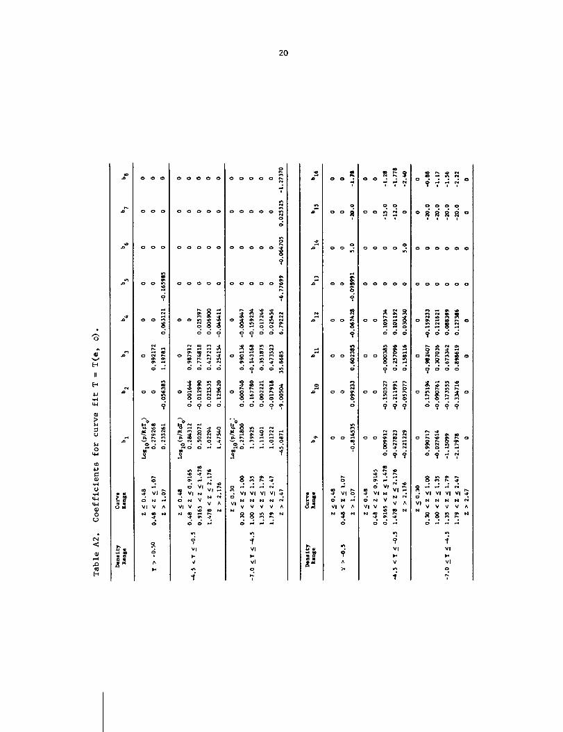
ficients bl, b2, ..., b16 are given in Table A2, Appendix A. These coef-
ficients were determined in such a manner as to compensate for the errors
incurred in the initial calculation of pressure using Eq. (2).
h = h(p, p)
For the correlation of h = h(p, p), the ratio y = h/e was curve-fitted
as a function of p and p so that h can be calculated from
h = (P/O (7)
Page 15
N
The general form of the equation used for y was
c5 + c6Y + c7Z + c8YZ
[( )]Y = Cl + c2Y + c3Z + c4YZ + I + exp c 9 X + Cl0Y + Cll
where Y = log10(P/l.292), X = lOgl0(P/l.013 X 105 ), and Z = X - Y. The
coefficients Cl, c2, ..., Cll are tabulated in Table A3, Appendix A.
T = T(p, p)
was
The general form of the equation used for the correlation T = T(p, p)
lOgl0(T/To) = d I + d2Y + d3Z + d4YZ + d5Z2
d 6 + d7Y+d8Z + dgYZ + dl0Z2
+ + +
where Y = log10(P/l.225), X = log10(P/l.O134 × 105), and Z = X - Y.
The coefficients dl, d2, ..., d12 are given in Table A4, Appendix A.
For the "time-dependent" method, the three curve fits p = p(e, p),
a = a(e, p), and T = T(e, p) have been placed in a single subroutine
named TGASo The calling sequence and FORTRAN IV listing of this subroutine
appear in Appendix B. For the "shock-capturing" method, the curve fits
h = h(p, p) and T = T(p, 0) have been placed in separate subroutines,
each named TGAS. These subroutines could be combined into a single sub-
routine, if desired, or could be used in their present forms in the same
computer program if one of the subroutines names were changed. The calling
sequences and FORTRAN IV listings of these subroutines appear in Appendix C
and Appendix D, respectively.
Page 16
COMI_ARISONSWITHRGASPROGRAM
Comparisonsof the curve fits p = p(e, p), a = a(e, p), T = T(e, p),
h = h(p, p), andT = T(p, p) with the original RGASprogramare shownin
Figs. 4, 5, 6, 7, and 8. In order to makethe comparisonsfor the first
three curve fits, the following procedurewasused. First, p and p data
were supplied, which allowed the original RGASprogramto computee. Then,
this e and the original pwere inputed into the TGASsubroutine to obtain
p, a, andT. Becauseof this procedure,pressure is plotted as one of
the independentvariables in Figs. 4, 5, and 6.
In order to assessthe relative accuraciesof the present curve fits
with the RGASprogram,500data points, along constant density lines ranging
from 103 to 10-7 amagats,were selected for a comparison. Themaximum
percentagedifferences betweenthe RGASandTGASprogramsalong eachcon-
stant density line are tabulated in Table i. Theaccuraciesof the present
curve fits are substantially improvedover the accuracies of the previous
curve fits appearingin NASACR-2134I. Themaximumpercentagedifferences
for the primary variables p = p(e, P) andh = h(p, p) were found to be
4.7%and4.6%, respectively.
A comparisonof the relative computertimes required for the TGAS
subroutines andthe NASARGASprogramson the IBM360-65computerare
given in Table 2. ThenewTGASsubroutine for finding p = p(e, p),
a = a(e, p), and T = T(e, p) is 2.68 times faster than the modified NASA
RGAS subroutine, as compared with the old TGAS subroutine which was 2.65
times faster. These comparisons do not include the time spent by the RGAS
subroutine in reading the tape. The new TGAS subroutine for finding
h = h(p, _ is 3.80 times faster than the original RGAS program as com-
pared with the old TGAS subroutine which was 3.88 times faster, again
Page 17
eo "¢.0.9__ o _
o_\ _ z,-
5
, I I, I J
_ X X _
0
o/o'OlI_ A£_I]N] NYNI]JJ_II
X
oop
X
•-- 0
o"
,-o__X
_c
o"v
II
0u.4
_J
I-i
0
0
0cO
Page 18
10
CNC)
X
.<O
.<Z__
1 , ,J lC) O
O
X
O P-
O/D 'OIJ._l CINrIOS dO 03ads
%
%
p_
%X
r-- O
- o"
-- X u.I
14.1
%m
?O
IO
F-. XIO "-
c_
v
II
0u_
4J°_I4.1
u
4-i0
0
°N
0
_g
°_
Page 19
11
v
II
0
,_
>I-I
0
',t-I
0
0
I-I
0
rj
Page 20
12
i
e_
1¢
o _-_ Z_--
II
=o
1 , 1 , I , I ,O O O O
e_O
4/14 _OllWl M'IVHJJxI_]
X"T
e.-
xi'm ,_1
Page 21
13
0
w.-
m
eD
m
o
-- × ,,_
p-
?O
I0
0
_(
II
0
c_
.,4
;>
u
0
0in
.,.-I
0
_d
.H
Page 22
14
Table I. Maximum percentage differences between RGAS and TGAS programs.
Density Curve Fit
ratio
0/0 ° p = p(e, p) a = a(e, p) T = T(e, p) h = h(p, 0) T = T(p, p)
103 2.2% 2.0% 3.9% i .8% 2.3%
102 1.3 1.0 2.5 1.4 3.0
I01 1.5 1.3 3.3 1.9 2.6
I00 1.8 I.i 2.9 2.2 2.0
I0 -I 2.5 2.7 4.4 2.4 2.9
10 -2 2.9 1.4 3.0 2.9 1.9
10 -3 3.7 3.2 4.1 3.3 2.8
10 -4 4.7 2.9 5.3 3.9 2.2
10 -5 3.9 3.2 3.1 4.2 2.5
10 -6 4.0 3.7 4.0 3.3 4.3
10 -7 4.2 5.9 4.4 4.6 3.4
Table 2. Comparison of computer times.
Number of Old New
Curve Fit Data Points TGAS TGAS RGAS
p = p(e, p)
a = a(e, p)
T = T(e, p)
5080 6.04 sec 5.98 sec
3.73 sec (data point 0-I)
includes tape read
16.01 sec (data points 2-5080)
19.74 sec
h = h(p, D) 5096 2.61 sec 2.67 sec
2.80 sec (data point 0-I)
includes tape read
10.12 sec (data points 2-5096)
12.92 sec
Page 23
15
excluding the tape read time. If there are only a fewhundredcalls made
to these real gas subroutines, then the TGASsubroutines are substantially
faster than the RGASsubroutineswhenthe tape read time is included. For
instance, if there are 500 calls madeto find p = p(e, P), a = a(e, p) and
T = T(e, P), then the newTGASis 8.95 times faster than the modified RGAS
subroutine.
Comparisonsof the values obtained at the juncture points of adjacent
curve fits (see Fig. 2) are shown in Table 3. The maximum deviations
between the curve fits at the juncture points of the primary variables
p = p(e, p) and h = h(p, 0) are 0.81% and 0.98%, respectively.
The simplified curve fits developed in this study for the thermodynamic
properties of equilibrium air allow the user to reduce computer time and
storage while maintaining good accuracy. This is particularly true in the
"time-dependent" method, since the simplified curve fits could be used
until near the end of a calculation when the "steady-state" solution is
approached. Then, the modified RGAS subroutine could be used to give more
accurate thermodynamic properties for the final steps. Substantial savings
in computer time may also result in the "shock-capturing" method since an
iterative procedure involving h = h(p, p) is required for equilibrium
calculations.
Page 24
16
Table 3. Comparison of variables at juncture points.
Density Point A Point B Point C Point 0 Point ECurve ratlo
Fit _0 ° Lower Upper Lower Upper Lower Upper LoWer Upper Lower Upper
10 3
10 2
I01
I0 °
i0 -I
p = p(e, p) 10 .2
10 .3
10 .4
i0 "5
10 .6
10 .7
1,400 1.393 1,294 1.293 1,228 1.231
1.400 1,393 1,287 1,286 1,208 1.210
1,400 1.393 1.280 1,279 1.187 1.189
1.400 1.393 1.273 1.272 1.166 1.168
1.400 1.395 1.300 1.298 1.185 1.185 1,153 1.[52
1.400 1.395 1.284 1.284 1.173 1.167 1.141 1.138
1.400 1.396 1.270 1,271 1.159 1.150 1.127 1.124
1,400 1.396 1.257 1.257 1.144 1.112 I.II3 I.II0
1.400 1.397 1.259 1.257 1.131 1.139 1.089 1.094 1.125 1.125
1.400 1.397 1.245 1.240 1.125 1,128 1.083 1,086 1.115 1.115
1.400 1.398 1.233 1.223 1.119 1,117 1,076 1.077 I.I05 1.105
103 443
102 443
I01 443
100 443
I0 "L 443
• = a(e, p) IO -2 443
10 -3 443
10 "4 443
10 .5 443
10 -6 443
10 "7 443
438 364 359 314 314
438 356 352 296 297
438 349 346 279 279
438 341 339 260 260
437 357 355 267 271
438 346 345 255 258
438 334 334 242 244
438 323 323 227 229
440 294 316 221 226
440 291 304 216 216
441 289 292 211 206
250 252
238 239
224 225
210 211
186 191
179 181
172 171
218 224
210 212
201 203
103
102
i01
i00
lO -I
T " T(e, 0) 10-2
10 -3
10 "4
10 -5
10 -6
10 -7
5.73 5.69 14.87 14.95
5.73 5.69 14.87 15.03
5.73 5.69 14.87 15.02
5.73 5.69 14.87 15.00
5.74 5.71 15.42 15.93 42.28 41.98 109.2 106.6
5.74 5.69 15.36 15.56 39.46 39.17 98.56 95.77
5.74 5.67 15.30 15.21 36.82 36.55 88.92 88.26
5.74 5.65 15.25 14.86 34.36 34.10 80.23 82.20
3.79 3.74 16.50 16.50 28.92 28.97 51.05 53,28 126.3 126.9
3.79 3.74 16.11 16.14 27.34 27.37 48.99 50,00 119,2 119.8
3.79 3.75 15.72 15.79 25.86 25.85 47.00 46.92 112.5 112.1
i03
102
101
i00
10 -I
h - h(p, O) 10"2
i0 "3
I0-4
10 .5
10 -6
10 .7
1.400 1.404 I. 291 I. 294 I. 253 1. 255
1.400 1.404 1.282 1.284 1.231 1.233
1.400 1.403 1,272 1.274 1.210 1.211
1.400 1.403 1.262 1.263 1.188 1.189
1.400 1,397 1.313 1.312 1.203 1.204 1.155 1.155
1,400 1.397 1.287 1.287 1.191 1.183 1.140 1.137
1.400 1.397 1.262 1.262 1.171 1.163 1,124 1.121
1.400 1.397 1.236 1.238 1.148 1.144 1.I07 I.I06
1,400 1.384 1.292 1.301 1.159 1.156 1.104 1.104
1,400 1.387 1.260 1.259 1.142 1.138 1.093 1.092
1.400 1.389 1.228 1.217 1.125 1.121 1.083 1.080
lO 3
lO 2
i01
100
10 -1
T - T(p. p) 10 .2
10 -3
10 -4
10 .5
i0 -6
10 -7
5.720 5.681 14.96 14.91
5.720 5.681 14.96 14.96
5.720 5.681 14.96 15.01
5.720 5.681 14.96 15.06
5,736 5.698 15.42 15.86 42.59 42.09 109.2 109.0
5.736 5.682 15.37 15.57 39.74 39.45 98.77 98.49
5.736 5.665 15.33 15.28 37.07 37.01 89.34 88.95
5.736 5.649 15.28 15.00 34.59 34.73 80.80 80,33
3.810 3.738 18.51 18.47 36.34 35.98 83.50 83.90
3.810 3.738 18.32 18.33 35.60 35.44 82._5 82.45
3.810 3.738 18.13 18.20 34.92 34.94 81.35 80.95
Page 25
17
REFERENCES
i. Tannehill, J. C. and R. A. Mohling, "Development of Equilibrium Air
Computer Programs Suitable for Numerical Computation Using Time-Dependent
or Shock-Capturing Methods," NASA CR-2134 (September 1972).
2. Lomax, H. and M. Inouye, "Numerical Analysis of Flow Properties About
Blunt Bodies Moving at Supersonic Speeds in an Equilibrium Gas,"
NASA TR R-204 (July 1964).
3. Kutler, P., W. A. Reinhardt, and R. F. Warming, "Numerical Computation
of Multishocked Three-Dimensional Supersonic Flow Fields with Real Gas
Effects," AIAA Paper 72-702 (June 1972).
4. Barnwell, R. W°, "Inviscid Radiating Shock Layers about Spheres
Traveling at Hyperbolic Speeds in Air," NASA TR R-311 (May 1969).
5. Grabau, M., "A Method of Forming Continuous Empirical Equations for
the Thermodynamic Properties of Air from Ambient Temperatures to
15,000 OK with Applications," AEDC TN-59-I02 (1959).
6. Lewis, C. H. and E. G. Burgess, "Empirical Equations for the Thermo-
dynamic Properties of Air and Nitrogen to 15,000 °K," AEDC TDR-63-138
(1963).
Page 27
19
APPENDIX A Coefficients for curve fits
o
O_
v
m
II
a_ ,"
IJ
.Mtl..l
Qt>
U
0
4..I
0
U
• 0 . .
?o? ?o?? ??o
o o
oooo ooooo o_ooo_
o ..... _ooo_o ?
ooooo o_ooo_
i
?o?o ???oo
,°°, 0,,,°
???o ????_
• °
vivi_ _ vlvivl_ _ vlvlvlVl
vl v v ^ vl v v v ^ vl v v v v ^
VI Vl
^ v vl
o o o
o_0_o"
_o_
oi!i
°lllo??
_o_ill
°R_
Ill
o o
lvlvl_
vl V V ^
,,
?^
o_1• . • .
?o??
0000
°flo_• 0 ° 0
?ooo
o_o°°°°
T??T
o o o o o
?
oo_
o_Iiii
o_o ? o o
o_g_• . . .
.-, ,,; <..i,_ vi vlviI_
Vl V V V #%
• • •
o?Vli-
V
in
,°..°
o??o?
• ° ° • •o o o o o
• ° • • •
? o o o o
oo_o• . °
i ! I
oo_88o? o,"?"
oooo_o
o o o• , °
oo_,_oo
oo_oo o _
oo_o
• ° • •
vl vl vl vl¢_ i_1 i,i el N e.I
Vl v v v v ^
vl
Page 28
2O
O_
[-_
II
E_
4-I
u_
:>
U
0
r_
¢.I
u_
u_
0C_)
<
-.t ).a i
e •
9u_
?
o
• °o .-4
°°_
?
.%
o •,-,o _
Vl v A
N _ N
o
0
A
ooooo
oooo
• , . o
v_
ooooo_
t
ooooo_
o o o o o _
o o o o o _
oo, o, oo_
• ° 0 . 0
ooo?.,
__ o .....
i VI
J N N °
_ V V
VI V _ _0 N
,7,Vl
V
...°
IVVVVA
• , ° .
Vl
Vl
g •
oo=.i..¢ ,m
o
oo o •
v_
o o ¢r1
o,
,4"
?
o
B
o
o o _s
o
o N ,-4
VI V A
0o
oo :_,_
o o• °
oo_o
oo o o o •
• . 0o o o
o?o,
,,-4 0
V Vl Vl
I e.,1I V .'-,
,_ ¢o N
c; c; .-,
c?Vl
0 • • • • 0
oooooo
_ooo
• 0 • .
o o o
0...
o???
• . ° •
°?yV
• , • °
t_l N I,.1 t,,.I _1VI
V V V V A
• • • •
..1
Vl
o
Page 29
21
Table A3. Coefficients for curve fit h = h(p, p).
T
Density Curve
Range Range el c2 c3 c4 c5 c6
¥ > -0.50
z _ 0.30 1.40000 0 0 0 0 0
0.30 < Z < 1.15 1.42598 0.000918 -0.092209 -0.002226 0.019772 -0.036600
1.15 < Z _ 1.60 1.64689 -0.062155 -0.334994 0.063612 -0.038332 -0.014468
Z > 1.60 1.48558 -0.453562 -0.152096 0.303350 -0.459282 0.448395
-4.50 < Y _< 0.50
z _ 0.30 1.40000 0 0 0 0 0
0.30 < Z _ 0.98 1.42176 -0.000366 -0.083614 0.000675 0.005272 -0.115853
0.98 < z _ 1.38 1.74436 -0.035354 -0.415045. 0.061921 0.018536 0.043582
1.38 < Z <- 2.04 1.49674 -0.021583 -0.197008 0.030886 -0.157738 -0.009158
Z > 2.04 1.10421 -0.033664 0.031768 0.024335 -0.176802 -0.017456
-7 < Y < -4.5
Z _< 0.398 1.40000 0 0 0 0 0
0.398 < Z <_0.87 1.47003 0.007939 -0.244205 -0.025607 0.872248 0.049452
0.87 < Z <_1.27 3.18652 0.137930 -1.89529 -0.103490 -2.14572 -0.272717
1.27 < Z _ 1.863 1.63963 -0.001004 -0.303549 0.016464 -0.852169 -0.101237
Z > 1.863 1.55889 0.055932 -0.211764 -0.023548 -0.549041 -0.101758
Density Curve
R_nge Range c7 c8 c9 Cl0 Cll
¥ > -0.50
Z _ 0.30 0 0 0 0 0
0.30 < Z < 1.15 -0.077469 0.043878 -15.0 -I.0 -I.040
1.15 < Z < 1.60 0.073421 -0.002442 -15.0 -1.0 -1.360
Z > 1.60 0.220546 -0.292293 -10.0 -1.0 -1.600
-4.50 < Y _< 0.50
Z _ 0.30 0 0 0 0 0
0.30 < Z _ 0.98 -0.007363 0.146179 -20.0 -1.0 -0.860
0.98 < Z < 1.38 0.044353 -0.049750 -20.0 -1.04 -1.336
1.38 < Z <-2.04 0.123213 -0.006553 -I0.0 -1.05 -1.895
Z > 2.04 0.080373 0.002511 -15.0 -1.08 -2.650
-7 <_Y__<-4.5
Z _ 0.398 0 0 0 0 0
0.398 < Z _0.87 -0.764158 0.000147 -20.0 -1.0 -0.742
0.87 < z _ 1.27 2.06586 0.223046 -15.0 -1.0 -1.041
1.27 < z <- 1.863 0.503123 0.043580 -10.0 -1.0 -1.5_4
Z > Z 1.863 0.276732 0.046031 -15.0 -1.0 -2.250
Page 30
22
C)-
v
II
[--,
u_
U
0u_
c_.IJ
Q)°e..l
U-H,4.4
u_
0
cO
J
a)
c_
_)
.I::i
N
'0
qu
q
0
0 r_
,-.4
r_
0 -,I"
!
O0
°;_0
¢_1 ¢h_0 ,-4O _OO
O ,-_
o -,1-O
I
0
0
Vl_
N _V ^
0
0
0I
^
en ,4" 00 r-. ¢_ 0
0 ,4" 0
I ! I
0 O 0 0
r,. ¢_i i_.
!
,,o _r_ cN 00
O0 ¢_ eq ,.I"
O0
_h O0 -,I' I'_
_ _ _ 0_ _ _ 0N N _ _
oo_
I I
,-I _ O0
CO u_ ..I' ,..4
N ,,,1" 0 ,.I"
O 0 ,-_ 0
_0u'_ t',,
• Vl _
v vlI N
N V _ dV
V in A
!
Vl
V
.gI
0 t_ _,_ ,,1"• ,1" _ _h ao¢_1 0 00 N
0 O 0 0
C_ ,-I ",1' ,.-4
0 0 O
0 0 0 0! !
,-I O
00 ¢_ 00 00
O_ ,.4
_ N N
°o_O O O O
! I
_°_
0 u'_ N
Vl Vl v_ NN N N ¢N
V V V A
¢_ O u'l
O ,_ ,.4
I
Vl
V!
!
N_4
'O
O
"O
_h
"O
CO'O
"O
.,4
mm
a0
i
O
o
!
a0
,,1"
O ,..4_C_l
c_I
O_
CO
o'IO 00
O
O!
a0a0O_
O 00O
erl_O
c_
vOI o_
N O
V A
CO N
O
I
A
00
00 ,--o0 _ ,"4
I l I
O O O
I I I
O O O O
_0 _ _,_ OO ,=4 O O
_ ",,1" _
O O O
,=4 ,.4 N
a0 O_ O¢h _0 Oh
O _0 Oh
I I I
_0
Vl ._VI N
N c_l
N V V AV _n
O O ,'_
O!
Vl
V
!
I I I I
O O O O
I I I I
O O O O
O O_ ,..4 u'_I'_ ;'_ er_ O_O ,..4 _ ,_
I I I I
U'_ ¢_ O
•-,1" U'I ,-4 _)
I I I I
0 N 00
00 _ID ,...I
O u'_ N
vl vl vlN N N
V V V A
!
Vl
vl
I
Page 31
23
APPENDIX B
SUBROUTINE TGAS FOR p = p(e, p), a = a(e, p), and T = T(e, p)
with
The calling statement for this subroutine is
CALL TGAS (E, RHO, P, A, T)
E = Internal energy, m2/sec2-
RHO = Density, kg/m 3
P = Pressure, newtons/m 2
A = Speed of sound, m/sec
T = Temperature, OK
The following logic can be employed when the English system of units is
desired:
E1 = E * 0.0929
RHOI = RHO * 515.4
CALL TGAS (El, RHOI, PI, AI, TI)
P = PI * 0.02088
A = AI * 3.281
T = TI * 1.80
with
E = Internal energy, ft2/sec 2
RHO = Density, slugs/ft 3
P = Pressure, ibs/ft 2
A = Speed of sound, ft/sec
T = Temperature, OR
Page 32
24
Listing of TGAS for p = p(e, p), a = a(e, 0), and T = T(e, p)
SUBROUTINE TGAS(E,RHO,P,A,TI
Y2=ALOGIO(RHO/I.292)
72=ALOGlOIE/78408.4}IF(Y2.GT.-.50} GO TO IIIFIY2.GT.-4.50) GO TO 6
IF(Z2.GT..65) GO TO l
GAMM=I.400
SNDSQ=E*,560GO TO 1B
I IFIZ2.GT.I.50) GO TO 2GAMM=I.46543+(.OO7625+.OOO292*Y2)_Y2-(.254500+.OI7244_Y2)*Z2
A+(.355907+.OIB422=Y2-.163235_Z21*Z2=Z2
GAME=Z.304_I-.25450-.OI7244w=Y2+(.711814+.OBO844=Y2-.489705=Z21*Z2|GAMR=2.304_(.OO7625+(-.O17244+.OI5422=Z2)*Z2+.OOO584_Y2!A1=-.000954
A2=.171187
A3=.004567GO TO 17
2 IF(Z2.GT.2.201 GO TO 3GASI=Z.OZ636+.O584931Y2
GAS2=.454886+.O27433_Y2GAS3=.165265+.O14275_Y2GAS4=.I36685+.OIOO71_Y2
GASS=.O5849B-.O27433_Z2
GAS6=-.01427 5+.OIOOTIIZ2GAST=EXP|O.285*Y2-30.O_Z2+58.41)
DERE=-BO.ODERR=0.285A1=.008737A2=.184842A3=-.302441GO TO 15
3 IF(Z2.GT.3.05) GO TO 4
GASI=I.60804+.O3479I_Y2GAS2=.188906+.OlO927_Y2GAS3=.124117+,OO7277_Y2GAS4=.O69839+.OO3985*Y2GAS5=.O34791-.OlO927_Z2GAS6=-.OO7277+.OO3985_Z2GAS7=EXP(O,21_Y2-30.O_Z2+80.731DERE=-30. OOERR=O,21A1=.017884A2=.153672A3=-,930224GO TO 15
Page 33
25
4 IF(Z2=GT.3°38! GO TO 5
GASl=l.25672+. 007073.Y2
GAS2 =. 039228-. 000491"Y2GAS3=-° 721798-=073753.Y2
GAS4=-. 198942-.021539*Y2
GAS5=. 007073+= 000491= 72
GAS6 ==073753-,, 021539"Z2
GAS7=EXP(O.425*Y2-50.0.Z2+166° 71
DERE=-50.O
DERR=O°325A1=.002379
A2=° 217959
A3=°005943
GO TO IS
5 GAMM=-84.0327÷(-.83176I+.OOII53*Y2}_=Y2÷(72.2066+.491914*Y2}*Z2
A* (- 20. 3559-. 070617_Y2_ I. 90979"Z2 }*Z2"_=2
GAME=2. 304" !72.2066+.491914"Y2+(-40.7118-. I41234"Y2+5. 72937"Z 2)
A*Z2_
GAMR=2,, 304* (-. 831761+. 002306.Y2+(. 49191k-. 0706 17*Z21*Z2)
AI=.006572
A2=. I83396
A3=-. I35960
GO TO I7
6 IF(Z2.GT°.651 GO TO 7
GAMM= 1.400
SNDSQ=E*. 560
GO TQ iQ
7 IF(Z2.GT.I.54| GO TO 8
GASI =I. 448 I3+. 001292"Y2
GAS 2:.0735 I0+. 001948*Y2
GAS3 =-. 05/+745+.013705"Y2
GAS4=-. 055473+. 02i 874,Y2
GASS=.O012g2-. 001948*Z2
GAS6=-. 013705+.021874"Z2
GAS7=EXP(-IO.O*(Z2-1°42)|
DERE=-1.0
DERR=O.O
AI=-.001973
A2=.I85233
A3=-. 059952
GO TO 15
8 IF(Z2.GT.2°22| GO TO 9
GA S I = I • 73158+,, 003 902* Y2
GAS2=. 272846-. 006237=Y2
GAS3=-. 041419-.037475"Y2
GAS4=. 0169 84-. O18038=Y2
GAS5 =. 003902+.006237"Z2
GAS6=. 037475-. 018038"Z2
GAS 7=EXP | ( -tO. +3. O_'Y2 I*( Z2- • 025"Y2- 2. 025| )
DERE=3. O_Y2-i 0.0
DERR=3. O*Z 2+12.15,Y2-20.325
AI=-.013027
A2=.074270
A3=.012889
GO TO 15
Page 34
26
9 IF{Z2.GT.2.90) GO TO i0
GAS I= I. 59350÷° 07532_Y2
GAS2=.I76186+.026072"Y2GAS3=. 200838÷. 05853_Y2
GAS6=.099687+. 025287"Y2
GAS5=.075326-. 026072"Z2
GAS6=-.O58536+.025287*Z2
GAST=EXP (-I0. O'Z2+ [5.0"Z2-13.5 )*Y2+27.0)OERE=5.0*Y2- IO.O
DERR=5.0"Z2-13.5AI=.004362A2=.212192
A3=-. 001293
GO TO I5IO GASI=I. I2688-. 025957"Y2
GAS2=-. 013602-. 013772"Y2
GAS3=. 127737+. 087962"Y2
GAS4=. 043104+. 023547"Y2GAS5=-. 025957+. 013772"Z2
GAS6=-.087942+.O23547*Z2GAS7=EXPt-20.0*Z2÷{4.0*Z2-13.21*Y2+66.0)
DERE=-20.+4. O'Y2
OERR=4.0*Z2-I3.2A I=. 006368A2=.209716
A3=-. 00600I
GO TO 1511 IF(Z2.GT..65) GO TO 12
GAMM=I.400
SNDSQ=E*. 560
GO TO 18I2 IF(Z2.GT,1.68! GO TO 13
GASI=I.455 IO-° O00102w_Y2
GAS2=.OQ1537-.OOOI66*Y2
GAS3=-. I28667+.049454,Y2
GAS4=-.IOI036+.0335IB*Y2GAS5=-. 000102+.000166,Z2
GAS6=-° 049454+. 0335I 8, Z2
GAS7=EXP (-i5.* (Z2-I.420))
DERE=-I5.DERR=O.
AI=.000450
A2=.203892
A3=.I01797GO TO 15
Page 35
27
13 I_(Z2.GT.2.46| GO TO 14
GASI=[. 59608-.042426_Y2
GAS2 =. 192840-.0293 53_=Y2
GAS3=. 019430-. 00595/+_ Y2
GAS/+=.O 26097-. 006 I64_Y2
GA $5=- • 0/+2426 + • 029353'I= Z2
GAS6= •00595/+-- 006164_=Z2
GAST=E Xp (-I 5._= ( Z2-2. 050} )
DERE=-I5.
DERR=O.O
AI=-. 006609
A2--. I27637
A3=. 297037
GO TO 15
I/+ GASI=I. 54363-.049071_'Y2
GAS2=. 153562-. 029209_=Y2
GAS3=.32/+907+. 0775991Y2
GAS4=. I/+2/+08+. 02207I_Y2
GAS 5=-. 04907i+. 029209_Z2
GAS6=-. 077599+.02207IIZ2
GAST:EXP(-10. O,W( Z2-2. 708l I
DERE=-IO.ODERR=O.O
AI=-.O00081
A2 = .22660I
A3=. i70922
I5 GASIO=I./(I.+GAST}
I() GAS8=GAS3-GAS4=Z2
GASg=GA S81GA STIGA SI 0=_=2
GA MM =GAS I -GAS 2 _Z 2-GAS 8_'GA S I 0
GAME=2.30/+= (-GAS2+GAS4_GASIO÷GASg_DERE }
GAMR=2.30/+_=(GASS÷GAS6eGASIO÷GASg=DERR}
17 SNDSQ=E=(AI÷(GAMM-I.)e(GAMM÷A2_GAMEI÷A3_'GAMR)
18 A=SQRT(SNDSQ)
P=RHO*E* (GAMM-I.)
X2=ALOGIO(P/I.OI34E÷05)
Y2= Y2÷.02 3126/+
Z3=X2-Y2
IF(Y2.GT.-.50) GO TO 29
IF{Y2.GT.-/+.50) GO TO 2/+
IF(Z3.GT..30) GO TO 19
T=P/(287.WWRHO)
RETURN
19 IF(Z3.GT.I.OO) GO TO 20
T = 10 _WWW( • 2718 ÷. 00074wk Y 2÷ ( • 990136-. 00/+ 947_Y2 ) w_Z3 ÷ ( • 990717
A÷. 175194wwY2-(. 982407-*-. 159233,WY2|*Z31 / ( I.÷EXP (-20.'_( Z3-O. 88| ) ) )
GO TO 32
20 IF(Z3.GT.I.35| GO TO 21
T=IO_=_I I.39925+.I67780_Y2÷(-.I/+3168-.15923/+_Y21eZ3÷(-.02761/+
A-.OgO76I=Y2÷{.307036÷.I2162IeY2)eZ3|/{I.÷EXP(-20.e(Z3-I*I7) ))|
GO TO 32
2I T F(Z3.GT.I.79| GO TO 22
T=iO_=e( I. I I401÷.00222I_Y2÷|. 351875÷.OI7246tY2)_,Z3+(-I. I5099
A-.173555'kY2÷(.6733424-.OSB399=Y21_Z3|/(I°÷EXP{-20*=(Z3-1°56) I) I
GO TO 32
Page 36
2B
22 IF(Z3.GT.2.47) GO TO 23T= lOW_1( i. 01722-. 017918_'Y2÷(. 473523÷. 0254565Y2 )*23+ (-2. 17978
A-.3347161Y2÷(.898619÷.I27386(=Y2)'I'Z3)/(I.÷EXP(-20.ww(Z3-2.22))} |GO TO 32
23 T=lO_WW(-45,0871-9,00504(=Y2÷(35,8685+6,7922(=Y2)(=Z3-(6,77699A÷l,Z737wwY2)(=Z3(=Z3÷ (-, 064705÷,025325_'Z3)WwY2(=Y2)
GO TO 3224 IF(Z3.G'r..48) GO TO 25
T=P/(287._WRHO)
RETURN25 TF(Z3.GT..9165) GO TO 26
T=I OW,W,(. 284312+. 987912(=Z 3+. 001644_wY2 )GO TO 32
26 IF(Z3,GT,1,478t GO TO 27T=IO"WW( ,502071-,01299(=Y2÷(, 774818÷,025397(=Y2) (=Z3÷(, 009912
A-, ].50527(=Y24-(-, 000385÷, 105734(=Y2 |_wZ3) / ( 1,+EXP(-15,(=( 23-1 ° 28) ) | )GO TO 32
27 IFIZ3.GT.2.176) GO TO 28T=IOW_(=( i. 02294÷. 021535=Y2÷ |• 427213÷. O06900*Y2)wwZ3+ (-°427823
A-.211991'IcY2÷(.257096÷.lOIIq2(=Y2)_wZ3)I(1.÷EXP(-12._'(Z3-1.778))))
GO TO 3228 T=IO(=(=(I.47540÷°I2962W'Y2÷(.Z54154-.O46411*Y2)(=Z3÷(-.221229
A-. 057077w.Y2÷(. 158116÷.03043(=Y2)(=Z3 )/ (1._-EXP ( 5.(=Y2(=(Z 3-2.40) )) )
GO TO 32
29 IF(Z3.GT,,48| GO TO 30T=P/(287.(=RHO)RETURN
30 IF(Z3.GT.I.07) GO TO 31
T=10(=(=(. 279268÷. 992172(= Z3)
GO TCI 3231 T=IOWkWw(.2332605-.O56383(=y2÷(I.19783+.O6312I(=Y2-.165085(=Z31(=Z3÷(-.8
A14535÷. 099233(=Y2÷( .602385-. 067428wwY2 - .098991(=Z3)(=Z3) ! ( 1. ÷EXP( (AS.(=Y2-20. I(=( Z3-I. 78) I ) )
32 T= Te151.777778
RETURNEND
Page 37
29
with
APPENDIX C
SUBROUTINE TGAS FOR h = h(p, p)
The calling statement for this subroutine TGAS is
CALL TGAS (P, RHO, H)
P = Pressure, newtons/m2"
RHO = Density, kg/m 2
H = Enthalpy, m2/sec 2
The following logic can be employed when the English system of units is
desired:
PI = P/0.02088
RH01 = RHO * 515.4
CALL TGAS (PI, RHOI, HI)
H = HI/0.0929
with
P = Pressure, ibs/ft 2
RHO = Density, slugs/ft 3
H = Enthalpy, ft2/sec 2
Page 38
30
Listing of TGASfor h = h(p, p)
SUBROUTINE TGAS(P,RHO,H|
Y2= ALOGIO(RHO/I.292)
X2= ALOGIO(P/I.O13E+O5)
Z3= X2-Y2
IF (Y2 .GT. -.501 GO TO 10
IF (Y2 .GT. -4.501 GO TO 5
IF (Z3 .GT. °398| GO TO I
H= (P/RHO)_3.50
RETURN
i IF (Z_ .GT. 0.870) GO TO 2
GASI=I.47003+.ooTg39*Y2
GAS2=.244205+.O25607_Y2
GASB=-.ST2248-.O49452*Y2
GAS4=-.764158+.OOOI47_Y2
GAS5=EXP(-20. OO*(ZB-O.T42)!
GO TO 14
2 IF (Z3 .GT. 1.270) GO TO 3
GASI= 3.18652+.I37gBo_Y2
GAS2= 1.89529+.I03490.Y2
GAS3= 2.14572+.272717.Y2
G_S4= 2.06586+.223046.Y2
GASS=EXP(-IS.00*(Z3-I.04I|)
GO TO i4
3 IF (Z3 .GT. 1.863) GO TO 4
GAS1= 1.63963-.00100436_Y2
GAS2= .303549-.OI6463g_Y2
GAS3= .85216Q+.IOI237_Y2
GAS4= .503123*.0435801_Y2
GASS=EXP(-IO. OO_(Z3-1.544))
GO TO 14
4 GASI = 1.55889+.0559323*Y2
GAS2= .211764+.0235478"Y2
GAS3= .54gO41+.lO1758*Y2
GAS4= .276732÷.O460305_Y2
GAS5=EXP(-IS.00_(Z3-2.250||
GO TO 14
5 IF (Z3 .GT. .300) GO TO 6
H: (P/RHO)m3.50
RFTURN
6 IF (Z3 .GT. 0.980) GO TO 7
GASI:I.42176-.OOO366*Y2
GAS2:.O83614-.OOO677mY2
GAS3=-.OO5272+.II5853mY2
GAS4:-.OO73&3+.I46179IY2
GAS5=EXP|-20.OOm|Z3-0.860)|
GO TO 14
7 IF (Z3 .GT. l.3BO) GO TO 8
GASI=I.T4436-.O35354*Y2
GAS2=.415045-.O61921_Y2
GAS3=-.OI8536-.O43582*Y2
GAS4=.O443534-.O49750*Y2
GASS=EXP(-20. OO*(X2-1.O4*Y2-1.3B6))
GO TO 14
Page 39
3i
8 IF (Z3 ,GT, 2.040) GO TO 9
GAS1=I,49674-.O21583*Y2
GAS2=.lgTOO8-.O30886*Y2GAS3=°I57738+.OO9158*Y2
G_S4=.I23213-.OO6553*Y2
GAS5=EXP(-IO°OO*(X2-1.O5*Y2-1.895|)GO TO 14
9 GASl=I.IO421-.O33664*Y2
GAS2=-°O31768-.O24335*Y2
GAS3=.IT8802+.OIT456*Y2GAS4=.OBO373÷.OO2511_Y2
GAS5=EXP{-I5,00*{X2-I.O8*Y2-2.650)|GO TO 14
IO IF{Z3,GT.°300) GO TO II
H= (P/RHO)*3.50
RETURN
II IF_Z3.GT.I.I5) GO TO 12
GASI=I.42598÷.OOOgI@*Y2GAS2=.Og220Q*.OO2226*Y2
GAS3=-.Olg772_.O36600*Y2GAS4=-,O774694÷.O43878*Y2GAS5=EXPI-15.00*{Z3-1.040))GO 70 i4
I2 IF(Z3.GT.I.600} GO TO I3GASI=I.6468g-.O621547*Y2
GAS2=.334994-.O636120*Y2GAS3=.O383322*.OI44677*Y2
GAS4=.O734214-°OO24417*Y2
GASS=EXP(-15.00*{Z3-I.360)}
GO TO 14
I3 GASI=I.48558-.453562*Y2GAS2=.I52096-.303350*Y2
GAS3=.459282-.44B395*Y2GAS4=.220546-,292293*Y2
GAS5=EXP(-IO.OO*(Z3-I.600))I4 GASIO= I./(I°*GAS5)
GAMM=GASI-GAS2*Z3-(GAS3-GAS4*Z3)*GASIOH=(PIRHOI*|GAMMI(GAMM-I.))
RETURNEND
Page 40
32
with
APPENDIX D
SUBROUTINE TGAS FOR T = T(p, 0)
The calling statement for this subroutine TGAS is
CALL TGAS (P, RHO, T)
P = Pressure, newtons/m 2
RHO = Density, kg/m 3
T = Temperature, OK
The following logic can be employed when the English system of units is
desired:
with
PI = P/0.02088
RHOI = RHO * 515.4
CALL TGAS (PI, RHOI, TI)
T= TI * 1.80
P = Pressure, Ibs/ft 2
RHO = Density, slugs/ft 3
T = Temperature, OR
Page 41
33
Listing of TGAS for T = T(p, p)
SUBRObTINE TGAS(P,RHC,T)Y2=ALOG IO(RHO/1.225!
X2=ALCGIO(P/I.O134E÷05)
Z3=X2-Y2
IF(_2.GT.-.50! GO TO 28
IF(Tr2.GT.-4.50) GO TO 23
I_(ZB.GT..30| GO TO 19
T=P/(287.W'RHO)RETLRN
19 IF(ZB.GT.I.07) GO TO 20
T =10'_'_(2. 72064+.00 B725'WY 2+ (. _38E5 I-. 01192W, Y2) w'Z3+ (. 682406+A. C89153"Y2-( .646541+. 070769_Y2)'WZB|/(I.+EXP |-20.'_(Z3-0.82) ) ||
GO ro 32
20 IF(Z3.GT.I.S7) GO TO 21
T=10,_,_(2.=_0246-.O42827w=Y2+| I. 12924+.041517w=Y2)w, Z3+|I.72067+
A.268OOBWWY2-(1.25038+.ITgT11,PY2),_Z3)/(I.+EXP(-20._,|Z3-1.33)|))
GO fO 3221 IF(Z3.GT.2.24) GO TO 22
T =10,v,k(2.44531-.047722w_Y2+ (1.00488+. 034349w_Y2)wwZ3+( 1.95893+
A.316244w, Y2-( I.OI2CO+.151561w, Y2)_WZBI/(I.+EXPI-20.,wIZ3-1.88))))G(] T0 32
22 T=IOWWWW( 2.50342+.026825*Y2+(.838860-.0(]9819_Y2)wwZB+{B.58284+
A.-=BB853w'Y2-(I.B6147+.I95436=_Y2|WWZB|/(I.+EXP(-20._'(Z3-2.47))))CO TO 32
23 IF(ZB.GT..48) GO TO 24
T=P/(28 7.'_RHO)RFTURN
24 IF(ZB.GT..51651 GO TO 25
T =lOW_W_(. 2816 11+. 9qO406W=Z3+. 001267w'Y2)
GC TO 3 125 IF(Z3.GT.1.478) GO TO 26
T= lOW,,v(.457643-. 034272_'Y2+( • 819119+. 046471'WY2)_,Z3+(-.O73233-Q.169816w, Y2+(.O432E4+.lI18_4w, Y2),_ZB|/(I.+EXP(-15.,_(Z3-1.28))))
GO TO 3126 IF(Z3.GT.2.1761 GO TO 27
T =10_'_( 1. 04172+. 04196 IW=Y
A. 1_6914*Y2+ ( .264883+. I0C
GO TO 3127 T=IO_W,(.4182_8-.252100_,Y2+(.784048+.I44576,WY2),_Z3+(-2.00015-
A.E390221wY24(.716053+.20_457w, Y2)'_ZB)/(I.+EXP|-IO.W,(Z3-2.40))))GO TO 31
28 IF(ZB.GT..48| GO TO 29T=P/(287.'_RH0)
RE rURN
29 IF(Z3.GT.._O) GO TO 30
T=IC_(.27407+I.0C082.Z3)
GC TO 3130 T=lOW,_,(.23586q-.O_3304w, Y2+(1.17619+.O46498w, Y2-.143721sZ3)W_Z3+
A (-1. 3767+. 160465'wY2÷ (I. C 8588-. C83489w_Y2-. 217748_,Z3| _,ZB) /
A ( I,+EXP (-I0._ =(Z3-I.78) I) )
31 T=T*273,232 T=¥/1.8
RETLRNEND
2÷(.412752-.O09329_Y2)=ZB+(-._34074-
5_gtY2)_ZBI/(I.+EXP(-15._(Z3-1.778))))
NASA-Langley, 1974