NASA-CR-3557 19830002376 NASA Contractor Report 3557 Technology Needs Assessment of an Atmospheric Observation System for Multidisciplinary Air Quality I Meteorology Missions Part 2 PC)"r\ .il. 11. r. "";- .. .... _"--"'-'-'J " l I .... 1 " • ..... __ -. .... ..... "I Ifo:r TO IlE 'l"I.iX!11 fi..;!/i 1il13 ROOt" U. R. Alvarado, M. H. Bortner, R. N. Grenda, W. F. Brehm, G. G. Frippe1, F. Alyea, H. Krniman, P. Folder, and L. Krowitz CONTRACT NASI-16312 SEPTEMBER 1982 NI\S/\ 1111111111111 1111 111111111111111 1111111111111 NF02137 ! I J -1 l l , https://ntrs.nasa.gov/search.jsp?R=19830002376 2018-06-15T08:08:29+00:00Z
Transcript
NASA-CR-3557 19830002376
NASA Contractor Report 3557
Technology Needs Assessment of an Atmospheric Observation System for Multidisciplinary Air Quality I Meteorology Missions Part 2 PC)"r\
.il. 11. r. "";- .. ~.......--~ -~-~ .... _"--"'-'-'J
" l I.... 1 ~ " • ..... ~---"'- __ -. .... -~ ..... "I ~~
Ifo:r TO IlE 'l"I.iX!11 fi..;!/i 1il13 ROOt"
U. R. Alvarado, M. H. Bortner, R. N. Grenda, W. F. Brehm, G. G. Frippe1, F. Alyea, H. Krniman, P. Folder, and L. Krowitz
Technology Needs Assessment of an Atmospheric Observation System for Multidisciplinary Air Quality I Meteorology Missions Part 2
U. R. Alvarado, M. H. Bortner, R. N. Grenda, W. F. Brehm, G. G. Frippel, F. Alyea, H. Kraiman, and P. Folder General Electric Company Philadelphia, Pennsylvania
L. Krowitz Lowell Krowitz Associates Philadelphia, Pennsylvania
Prepared for Langley Research Center under Contract NASl-16312
NI\S/\ National Aeronautics and Space Administration
Scientific and Technical Information Branch
1982
FOREWORD
The "Technology Needs Assessment of an Atmospheric Observation
System" reported in this contractor report for "Multidisciplinary
Air Quality/Meteorology Missions" and in a companion report for
"Tropospheric Research Missions" (NASA CR 3556, 1982) was funded
by NASA's Office of Aeronautics and Space Technology to derive
information necessary to guide near-term technology developmental
activities in support of NASA's Office of Space Science and
ANALYSES OF INCIDENCE ANGLES, SPECTRAL RADIANCE AND ORBITS .
5.1 5.2
Optical Radiance at Various Viewing Angles. Spatial Relationships ....•..... 5.2.1 Equatorial Coverage Frequency ....... . 5.2.2 Diurnal Cove~age .........•. 5.2.3 Effect of Incidence Angle on the
7.1 Payload Packaging and Dimensions. 7.2 Sensor Accomodation Parameters.
DATA MANAGEMENT SYSTEM . . . . . . . . . .
8.1 On-Board Segment of the Data Management System. 8.2 Ground Segment of the Data Management System ..
8.2.1 Functional Description of Ground Segment 8.2.2 Ground Data Management System Assessment. 8.2.3 Sizing of the Data ........•.. 8.2.4 Data Management System Issues ....•.
Page
4-30 4-30 4-41 4-42 4-42 4-45 4-46 4-47 4-48 4-48
5-1
5-1 5-20 5-20 5-24
5-27
6-1
6-4
6-7
6-10
6-11 6-13
7-1
7;-1 7-3
8-1
8-1 8-6 8-7 8-12 8-13 8-16
Section
9
10
TABLE OF CONTENTS (Cont'd)
TECHNOLOGY ASSESSMENT . . . . . . . . • . •
9.1 9.2
9.3
Technology Categorization .........• Description of the Technology Needs ........... . 9.2.1 Techniques to Increase Vertical Resolution
in Tropospheric Measurements ........... . 9.2.2 Measurement of Tropospheric Wind Vectors
Using Laser Heterodyne Spectrometry ..... 9.2.3 Improved Measurement of Sulfur Compounds:
H2S, H2 S03, SO, S03 .....•....... 9.2.4 Correlation of Ground and Space Observations
of the Effects of Aircraft Activity . . . • . 9.2.5 Measurement of Precipitation Parameters •.• 9.2.6 Spatial Correlation of Nadir and Limb Data .• 9.2.7 Passive Microwave Radiometer with
with Multispectral Linear Arrays. ~ ..... . 9.2.9 360 0 Scan Limb Sensors ....•........ 9.2.10 Improved Solar Shiel dings for Passive Sensors 9.2.11 LIDAR Techniques for Faint Species
in the Stratosphere • . . . . • • . . . . . . . 9.2.12 Doppler Radar for Precipitation Measurements. 9.2.13 Bi-Static Absorption Measurements ..... . 9.2.14 Sub-Millimeter Wave Sources for
Heterodyne Detectors ........•.... 9.2.15 DevE!'lopment of Algorithms for AOS Limb Data. 9.2.16 3-D Correlation of Air Quality and
Meteorological Parameters ...•...... 9.2.17 Interactive and Adaptive Mission Control ... . 9.2.18 Precise Attitude Control for Limb Measurements .. . 9.2.19 Assembly or Deployment of Large Passive
Appendix A Multispectral Linear Array Design Considerations.
Page
9-1
9-1 9-1
9-4
9-5
9-7
9-8 9-9 9-11
9-14
9-15 9-16 9-19
9-20 9-22 9-23
9-28 9-28
9-31 9-33 9-34
9-38 9-38
10-1
A-I
VI
SECTION 1 INTRODUCTION
Thi s report summari zes the resul ts of the study "Technology Needs Assesment of
an Atmospheric Observation System", performed for the NASA Langley Research
Center by the General Electric Company, Space Systems Division, under Contract
No. NAS-1-16312. Part I of the study dealt with Tropospheric Research
Mission and is published as NASA CR-3556.
This volume covers the results of Part II of the study, which deals with
multidisciplinary missions. The period of performance for Part II was
approximately eight months, commencing May 1981.
The purpose of the study was to defi ne the technology advancements needed to
support post 1990 space missions to perform global atmospheric measurements.
The study is not meant to define missions or assess science needs, but rather
to establish the boundaries of possibilities for technology and assess the
technology needs, a process which can only be effected through modeling and
planning of potential missions encompassing the mission disciplines, which are:
1. Tropospheric Air Quality
2. Upper Atmospheric Air Quality
3. Weather
4. Severe Storms
5. Air Surface Interface
The latter four disciplines are treated relative to their support of the
"core" mission, which deals with upper and lower atmosphere air quality.
Although the subject of the study is air quality, it is recognized that those
supporting measurements dealing with the physical state and dynamics of the
atmosphere are potenti ally useful to other operati onal meterological systems
by supplying to them complementary or corroborative data.
There are several reasons for the wide scope of the study, encompassing
multiple disciplines in a single space-based system. The technology
developments that may result from this study should have broad applicability
across several disciplines. Another reason is to make the modeled missions
1-1
upon which the study is based compatible with current trends towards using larger, more complex spacecraft. This in turn pennits us to examine the impact of these systems on technology.
From an applications point of view, the multidiscipline approach in the study pennits an examination of the potential synergistic benefits of simultaneous measurements of atmospheric quality and meteorological parameters.
Part II covers the following analyses:
1. Review of long-range NASA plans in atmospheric quality to detennine knowledge objectives and measurement needs. (Reference Section 3).
2. Detennination of the applicability of air quality measurements in the meteorological disciplines. (Reference Section 3).
3. Postulation of generic sensors that would be applicable to the measurement needs. (Reference Section 4).
4. Definition of the sensor characteristics. (Reference Section 4).
5. Synthesis of multidisciplinary space missions and the sensor complement characteristics. (Reference Sections 6 and 7).
6. Atmospheric model i ng and detenninati on of optical transmi ssion parameters for various angles relative to the local vertical. (Reference Section 5).
7. Definition of the field-of-view and incidence angle limits of various orbits based on the analysis in 6. (Reference Section 5).
8. Characterization of the relationship between passive sensor sensitivity and sensor design parameters such as optics size, and field of view. (Reference Section 4).
9. Examination of the synergistic benefits of multidisciplinary missions. (Reference Section 6).
10. Definition of the end-to-end data system for a typical multidisciplinary mission. (Reference Section 8).
11. Detennination of potential technology drivers in the end-to-end data system. (Reference Section 8).
12. Identification of the advanced technology needs in order to implement ·the mission in the early 1990 1 s. (Reference Section 9).
Ackno\'/ledgement: This study was sponsored by NASAls office of Aeronautics and Space Technology. Overall guidance and technical monitoring of the contract was provided by Lloyd Keafer of the Langley Research Center. Special guidance and meteorology mi ssi ons was provi ded by a group at the Goddard Space Fl i ght Center lead by Dr. S. Harvey Melfi.
1-2
SECTION 2
SUMMARY OF RESULTS
Thi s secti on of the report presents a capsul e summary of the resul ts of Part
II of the Atmospheric Observtion System Study.
The study showed that it could be .technologically feasible and sCientifically
pratical to launch multidisciplinary missions for atmoshperic research and
routi ne observati on, in the post 1989 era. Such mi ssi ons woul d benefit the
pursui t of knowl edge of the atmo spheri c envi ronment, not only from the poi nt
of view of air quality, but also weather, climate, severe storms and air
surface interface phenomena. The synergi sti c benefi ts of concurrent gas and
aerosol concentration measurements and meteorological measurements may
accel erate the fonnul ation of accurate atmospheric model s and thus permit us
to understand and control the effects of man1s activities upon our important
atmoshperic resources. As example of these synergistic benefits are the
simultaneous measurement of several gaseous/aerosol species, spectral regions,
and viewing geometries, which will enhance the accuracy of interpretation of
the chemical reactions ••
The technology developments identified by the study were not driven by the
fact that may sensors will be accommodated in one spacecraft. This is
evidenced by the fact that the size and system suppor trequired by the
postul ated payloads fall well wi thi n the projected capabi 1 i ti es of spacecraft
in the early 19901s. Rather, we found that the technology gaps center around
the sensing techniques and sensors, as they did in the Part I Study. It is
evident that the complexity of such detailed measurements in the upper and
lower atmosphere makes may of the measurements difficult relative to obtaining
theefrequent global coverage, with the required spatial resolution and
accuracy.
A list of the main technology developments that were identified in the study
are shown on Table 2-1. Indicated in that Table are the critical items
(asterisked numbers) \/hich require prompt attention to ensure that the
technology will be attained when it is needed by future environmental
satellites for atmospheric observation. It should be pointed out that these
technology needs are somewhat independent of the particular type of satellite
2-1
t-:l I
t-:l Table 2-1. List of Potential Technology Needs for ADS Multidisciplinary Missions
A) NEW MEASUREMENT TECHNIQUES
*1. TECHNIQUES FOR INCREASING VERTICAL RESOLUTION IN TROPOSPHERIC CONCENTRATION MEASUREMENTS. (e.g. LIMB MEASUREMENTS IN UPPER TROPOSPHERE)
2. MEASUREMENTS OF WIND VECTORS USING LASER HETERODYNE SPECTROMETRY
3. IMPROVED MEASUREMENT OF H2S04, HS03, H2S
4. CORRELATION OF GROUND & SPACE OBSERVATIONS OF THE EFFECTS OF AIRCRAFT ACTIVITY ( i . e., °3, NOx, CO)
5. MEASUREMENT OF PRECIPITATION PARAMETERS
6. SPATIAL CORRELATION OF NADIR AND LIMB DATA
B) PASSIVE SENSORS
*7. PASSIVE MICROWAVE RADIOMETER WITH FIXED, SHAPED REFLECTOR
*8. OPTICS FOR WIDE F.O.V. SENSORS COUPLED WITH MULTISPECTRAL LINEAR ARRAYS
9. 3600 - SCAN LIMB SENSORS
10. IMPROVED SOLAR SHIELDING FOR PASSIVE SENSORS
*CRITICAL TECHNOLOGY ITEMS
t\:)
I ~
Table 2-1. List of Potential Technology Needs for AOS Multidisciplinary Missions (Cont'd)
C) ACTIVE SENSORS & SOURCES
*11. LIDAR TECHNIQUES FOR FAINT SPECIES IN THE STRATOSPHERE
12. DOPPLER RADAR FOR PRECIPITATION MEASUREMENTS
13. BI-STATIC LIDAR MEASUREMENTS
14. SUB-MILLIMETER WAVE SOURCES
D) INFORMATION MANAGEMENT
*15. ALGORITHMS FOR AOS LIMB DATA
16. 3-D CORRELATION OF AIR QUALITY AND METEOROLOGICAL PARAMETERS
17. INTERACTIVE AND ADAPTIVE MISSION CONTROL
E) SPACECRAFT & SPACE ASSEMBLY
*18. PRECISE ATTITUDE CONTROL FOR LIMB MEASUREMENTS
19. ASSEMBLY OR DEPLOYMENT OF LARGE PASSIVE MICROWAVE ANTENNA ARRAY
system that will be employed to implement them. For instance, assuming that
none of the multidisciplinary atmospheric observation spacecraft postulated
here woul d be impl emented wi thi n the postul ated time frame, the technology
needs would still be valid under alternative scenarios. One of these
scenari os, for instance, woul d show advanced versi ons of the proposed Upper
Atmospheric Observation Satellite being complemented by a Lower Atmospheric
Research Satellite (LARS), and an effective information management system
gathering data from these two satellite systems, research aircraft and
advanced versions of current NOAA meteorological satellites. Under
alternative scenarios such as this, the technology gaps would still b.e
required to be filled, in most cases, within the relatively short time between
now and 1987.
2-4
SECTION 3 INFORMATION NEEDS
The problem of air quality has become a major environmental concern and should be aided by investigations based on global measurements from spacecraft. Hence, measurements pertinent to air quality are the major ultimate objectives towa rd whi ch thi s study is aimed. That is, thi s study is aimed towa rd the assessment of the technology needs for the eventual development of flight missions and their payloads which would provide the best possible measurements for the understanding, quantification, and subsequent improvement of the quality of the earth's atmosphere. It is not intended that this study develop the ultimate "knowledge objectives" as will have to be done for actual flight missions or to determine the best set of instruments, measurements, and flight parameters as will be done for such missions. Rather it is intended that such knowledge objectives, payloads, and missions as considered herein are intended only as representatives and are used only to permit a valid assessment of technology needs.
The objectives which should be pursued by measurements from orbiting spacecraft have been considered in detail by many scientists, committees, workshops, and others in order to furnish information on scientific needs to those involved in planning spacecraft missions. Some of the leading reports on the subject are listed in Table 3-1. These scientific objectives may be categorized in a number of possible ways; however, for the purposes of this study twel ve such "Knowledge Objectives" were de vel oped as shown on Table 3-2. There is obvious overlap in some of these objectives, but such can hardly be avoi ded in such a categori zati on. Materi al in references such as those of Table 3-1 was used for the obtention of information from which the knowledge objectives were generated.
3.1 KNOWLEDGE OBJECTIVES DEFINITION Each of the twelve knowledge objectives in Table 3-2 is made up of a number of parts, each of which is a sub-objective. Answeri ng all of the sub-objectives should provide an answer to that major knowledge objective. The breakdown of sub-objectives is shown in Tables 3-3 through 3-14.
3-1
Table 3-1. Documents That Form the Basis for the Knowledge Objectives * I Upper Atmosphere Research Satellite Science Working Group.
(Reference Number 1).
I The Stratosphere; Present and Future. (Reference Number 6).
I National Climate Program Five Year Plan. (Reference Number 7).
I Middle Atmospheric Program Planning Document. (Reference Number 8).
I Atmospheric Chemistry, Problems and Scope. (Reference Number 9).
I Space Remote Sensing of Minor Gaseous and Aerosol Components of the Atmosphere. (Reference Number 10).
I NASA Troposphere Program Plan. (Reference Number 11).
* Full references are given in Section 10.
3-2
Table 3-2. Knowledge Objectives
1. Effects of Pollutants on Atmospheric Radiative Transfer.
2. Atmospheric Sulfur Pollution.
3. Atmospheric Carbon Pollution.
4. Global Distribution of Ozone.
5. Effect of Aircraft Activity on the Atmosphere.
6. Effect of Chlorofluoromethane on the Atmosphere.
7. Effect of N20 on the Atmosphere.
8. Surface-Atmosphere Interaction.
9. Properties and Role of Atmospheric Aerosols.
10. Role of Ions in the Stratosphere.
11. Meteorological Effects on Atmospheric Composition and Radiative Transfer.
12. Effects of Natural and Man-Made Disturbances.
Table 3-3. Knowledge Objective 1
Effect of Pollutants on Atmospheric Radiative Transfer
1. Distribution of Effective Pollutants.
2. Effect of Pollutants on Ozone.
3. Effect of pollutants on Aerosol Size and Distribution.
4. Effect of Aerosol Size and Distribution on pollution.
5. C02 Concentration Trend.
6. Role and Effect of Water Vapor and Variations.
7. Variations in Resultant Solar Flux at Surface.
8. Terrestrial Radiation.
9. Effect of Pollutants on Cloud Cover.
3-3
3-4
Table 3-4. Knowledge Objective 2
Atmospheric Sulfur Pollution
1.
2.
3.
4.
5.
6.
7.
8.
S-Source Location and Quantification.
Identity and Distribution of S-Containing
Photochemistry of S-Containing Species.
Formation of S-Containing Aerosols.
Loss Processes of S-Containing Species.
Interaction with Aerosols.
Ac; d Rai n.
Troposphere-Stratosphere Transport.
Table 3-5. Knowledge Objective 3
Atmospheric Carbon Pollution
1. C02 Concentration Trends.
2. CH4 Photochemistr,y.
3. Natural Sources of CO.
4. Anthropogenic Sources of CO.
5. CO Sinks.
6. NMHC Photochemistry.
7. Troposphere-Stratosphere Transport.
8. Cross-Equatorial Flow.
Speci es.
Table 3-6. Knowledge Objective 4
Global Distribution of Ozone
1- Distribution of 03'
2. Variations in Distribution of 03'
3. Effect of Pollutants.
4. Photochemi stry.
5. Effect on Radiative Transport.
6. Surface Loss of 03'
7. Troposphere-Stratosphere Transport.
B. Effect of Atmospheric Electricity.
Table 3-7. Knowledge Objective 5
Effect of Aircraft Activity on the Atmosphere
1. Pollutant Distribution from Aircraft - e.g., NOX, HC's, CO.
2. Pollutant Interactions.
3. Pollutant Transport.
4. Effect on Ozone.
5. Effect on Radiative Transfer.
6. Effect on Cloud Cover.
Table 3-B. Knowledge Objective 6
Effect of Chlorofluoromethanes (CFM's) on the Atmosphere
1. Sources of CFMls.
2. Identity and Distribution of CFM's.
3. Sinks of CFMls.
4. Photochemistry of CFMls.
5. Effect on Ozone.
6. Effect on AtmospheriC Composition.
7. Troposphere-Stratosphere Transport. 3-5
3-6
Table 3-9. Knowledge Objective 7
Effect of N20 on the Atmosphere
1. Natural Sources.
2. Anthropogenic Sources.
3. Sinks.
4. Photochemistry.
5. N2 Distribution.
6. Troposphere-Stratosphere Transport.
7. Effect on Atmosphere.
Table 3-10. Knowledge Objective 8
Surface-Atmosphere Interchange
1. Ocean as a Source of Minor Atmospheric Constituents.
2. Ocean as a Sink for Minor Atmospheric Constituents.
3. Land as a Source of Minor Atmospher1c Constituents.
4. Land as a Sink for Minor Atmospheric Constituents.
5. Vegetation as a Source of Minor Atmospheric Constituents.
6. Vegetation as a Sink for Minor Atmospheric Constituents.
7. Aerosols from the Ocean.
8. Aerosols from the Desert.
9. Role of Wind and Transport.
Table 3-11. Knowledge Objective 9
Properties and Role of Atmospheric Aerosols
1. Size and Distribution of Aerosols.
2. Composition of Aerosols.
3. Interaction with Gaseous Components.
4. Interaction with Precipitation.
5. Formation Mechanisms.
6. Transport.
7. Effect on Radiative Transfer Properties.
Table 3-12. Knowledge Objective 10
Role of Ions in the Stratosphere
1. Identity and Distribution of Ions.
2. Gaseous Interactions.
3. Aerosol Interactions.
3-7
Table 3-13. Knowledge Objective 11
Meteorological Effects on Atmospheric Composition and Radiative Transfer
1. Effect of Temperature and Lapse Rate.
2. Water Vapor Interaction.
3. Chemical Effect of Lightning.
4. Effect of Clouds on Radiative Transfer.
5. Vertical Transport.
6. Horizontal Transport.
7. Transport by Wind.
8. Interaction of Precipitation with Atmospheric Species.
9. Removal of Pollutants by Precipitation.
10. PhYsical Effects of Severe Storms.
11. Field-of-View Effects of Clouds.
12. Surface Temperature and Terrestrial Radiation.
13. Interaction of Pollutants with Water Vapor.
Table 3-14. Knowledge Objective 12
Effect of Natural and Man-Made Disturbances
1. Effect of Gases and Condensed Material from Volcanoes.
2. Transport of Volcanic Material.
3. Atmospheric Interactions of Lightning.
4. Transport in Severe Storms.
5. Chemical Effects of Nuclear Bursts.
6. Radioactivity Introduced by Nuclear Bursts.
7. Effects and Uses of Chemical Releases.
8. Effects on Radiative Transport.
The first knowledge objective concerns the effect of atmospheric pollutants on the transmission, absorption, emission, scattering, reflection, and refraction of radiative flux. Many trace atmospheric species affect radiative transfer.
3-8
These include both naturally occurring and anthropogenically introduced species although these are, in general, the same with the anthropogenic effect being one of quantity, in some cases introducing possibly many more times the amount of a trace speci es than is naturally there. Many of these speci es affect the amount of radi ati on reachi ng the ground which in turn has major effects on both animal and vegetable life(8,14).
Among the species which are most important in their effect on radiative flux are 03' H20, and CO~6,8,9,1l) Small decreases in the total amount
of ozone in the atmosphere increase the solar flux penetrating the atmosphere, thus potentially increasing the incidence of skin cancer; therefore, there is great interest in the amount of ozone in the atmosphere. Since ozone is closely coupled with the photochemistry of many other trace species in the atmosphere, the distribution of the related species is of interest indirectly through the ozone problem as well as through the direct effect they may have on radiative flux. Some of the species most closely coupled with ozone photochemistry are NO, N02, N20, OH, H02, and Cl(3,8,11).
Aerosols play a major role in radiative transfer(6,11). They serve to absorb, reflect and refract solar radiation. Their size, number, and di stributi on are affected by and have an affect on atmospheric trace species. Much of this is not yet understood and it is difficult to be very specific about measurements needed to satisfy such a knowledge requirement until further technological advances are made. However, there is no doubt that aerosols must be characterized in tenus of size distribution and in tenus of number distribution before their effect on radiation can be predicted with assurance.
In conjunction with measurements of gaseous species and aerosols, as a function of time, altitude, latitude, and longitude, the detenuination of flux variations with these same parameters is needed.
Knowledge Objective 2 concerns sulfur pollution. This is an industrial pollutant and extensive measurements, mainly ground-based, have been made downwind from industrial sources. There is much less understanding of the ultimate fate of the sulfur thus introduced. Much of the sulfur is introduced
3-9
as H2S(6,13) (mainly from natural sources), S02 (mainly from industrial
sources), and CS2 and COS (from organic chemical processes). Through a
series of steps much of the sulfur ultimately is converted to H2S0i13)
Some reacts with ammonia(ll) to form (NH4)2 S04. These in turn are
fonned into aerosols. Much of it ultimately comes out as acid rain which
causes much interstate and international stress. It is important to follow sulfur emissions for long distances. It is necesssary to detennine the
chemical status of the sulfur, that is, to know what the distributions of
sulfur-containing species are as a function of time and location. In order to
understand the chemical conversions, knowledge of the distribution of chemical
constituents which react with sulfur-containing species is required. Chief
among these are OH, H02 and NH3 together with aerosols which interact
probably both chemically and physically with the S-contai ni ng speci es. The
characterization and distribution of the aerosols should be known and since
the sulfur becomes part of the -aerosol, the composition of the aerosol is
needed. The occurrence of precipitation should be included in any
sulfur-cycle study.
Some sulfur may enter the stratosphere. Some volcanoes introduce H2S and
sulfur in other fonns at high altitudes, sometimes even into the
stratosphere. Here, as in many other cases to be discussed later, the
interchange between the troposphere and the stratosphere must be understood.
Measurements for thi s type of process are difficul t to desi gn and must be
quite complex. Obviously, well-resolved measurements of sulfur-containing
species and aerosols are needed.
In studying troposphere-stratosphere interchange (which is important to many
of the knowledge objectives), the use of some species which is photochemically
unreactive in this region and which has a usable infrared spectrum has been
suggested as being a more feasible technique than temperature profile
determination. Methylchloroform, CH3CC1 3, has been suggested for this
purpose.
Knowledge Objective 3 concerns atmospheric carbon pollution. This involves
two or three rather distinct problems. One concerns the continual, gradual increase in CO2 wi th its resultant effect on radi ati ve fl ux (1,8). Thi sis
3-10
a very gradual change and can be investigated and followed by ground-based
measurements.
A second carbon-pollution problem is that of carbon monoxide. The natural
sources of CO are not yet understood. Thi s requi res an understandi ng of the atmosphere methane cycle and perhaps other similar cycles(6), as well as
determination of CO distribution with time, altitude, latitude (both
hemisphere) and longitude, with global coverage. To understand the methane
cycle, measurements of CH4 and, to the extent possible, numerous
intermediate species, are needed. Since OH is the most important species for
removing CO, it should also be measured. Data on winds, etc., which determine
transport are important to the understanding of CO, especially anthropogenic
CO.
In addition to methane, other hydrocarbons are significant to atmospheric
pollutions. These include the lower alkanes and those alkanes which are
present in significant quantities and certain other larger hydrocarbons which
may be introduced naturally or anthropogenically. Various terpenes are a
prime example of naturally introduced hydrocarbons whose fate is not well
known.
Knowledge Objective 4 concerns the distribution of ozone. This obviously
overl aps Knowl edge Objecti ve 1, but is specific for ozone and extends beyond
its effect on radiative transfer. Ozone is of great importance in the
stratosphere and its photochemistry involves many other species. Its
photodissociation is accomplished by UV radiation. This rate will vary with
time of day, time of year, and latitude since the solar flux varies in these
ways. Ozone, in turn, affects the sol ar fl ux, bei ng a major contri butor to
its absorption. Ozone, interacts either directly or indirectly, with most of
the minor atmospheric species which control many properties of the
atmosphere. It reacts directly with OH, H02, NO, N02, H, 0, SO, Cl, C10,
and others incl udi ng many anthropogenically introduced species. For many it
is the fastest destructi on mechani sm. It is of great importance to know the
distribution of ozone as a function of time and of altitude, latitude, and
longitude and to understand this distribution so that it can be predicted with
reasonable confidence for all conditions.
3-11
Several other factors must be considered in conjunction with this. The
atmospheric circulation of ozone is very complex. The role of troposphere
stratosphere interchange needs to be quanti tati vely understood, as does the
loss of ozone at the Earth's surface. The possible importance of the
well-known creation of ozone by lightning needs to be quantified.
Since the ozone problem is both very complex and very important, it will
require an involved program of measurements to satisfy this knowledge
objective.
Knowledge Objective 5 concerns the effect of aircraft activity on the
atmosphere. Ai rcraft burni ng fossil fuel s introduce the nitrogen oxides,
mainly NO and N02; unburned hydrocarbons; carbon monoxide and carbon
dioxide, and water. The most important influence is that of NO. It reacts
rapidly with ozone by NO + 03~ N02 + 02. It is not a one-for-one
effect, however, due to the very complex photochemistry of the 03-NOX
system. Various model s have predicted various effects on the ozone. It is
now generally agreed that there is some reduction in ozone due to the NOX
introduced by the ai rcraft.
In addition to the affect on radiative transfer due to ozone decreases, there
are effects on radiation due to the H20 and CO 2, and to a lesser extent,
the various other species introduced. These effects need studying by remote
measurements.
Since the aircraft activity is not globally unifonn, transport plays an
important rol e in the effect of ai rcraft-i ntroduced poll utants. The
understanding of the transport is a part of this objective.
Knowl edge Objecti ve 6 concerns the effect of chl orofl uoromethanes (such as
freon) on the atmosphere. For several years, chlorofluoromethanes have been a
concern to those involved with atmosphere processes. The original CFM's of
most interest were CF2C1 2, CFCL3, CHC1 3, and CC1 4• These and
various other CFMs are long-lived in the atmosphere. Most rise through the
trosophere and eventually enter the stratosphere. There they are
photodi ssoci ated and undergo a seri es of reactions which produce a number of
spec i es such as Cl, C10, HC1, and C10N02• Some of these react wi th ozone.
3-12
The process C1 + 03 - ClO + 02 appears to be important in reducing the
ozone burden in the atmosphere, thus affecting the sol ar f1 ux penetrati on.
Much of this remains to be quantitatively understood. It remains to
determine, for each of a dozen or so CFM1s, their distribution, their
transport from the troposphere to the stratosphere and wi thi n each of these regions, their lifetime in the atmosphere, the photochemical processes they
are involved in, including their reactions with and effect on ozone and their
reactions wtih nitrogen oxides, their interaction with aerosols, and their
overall effect on radiative flux. It is obvious that there needs to be
appropriate measurements of the distributions of many CFMs, and of many
species with which they interact and of various PhYsical parameters which
affect these distributions and processes.
Knowledge Objective 7 concerns the effect of nitrous oxide, N20, on the
composition of the atmosphere. The processes thought to cause such an effect are the following. Nitrogen-containing fertilizers are responsible for its
introduction into the atmosphere. Since it reacts extremely slowly with
tropospheriC species it has time to be transported into the stratosphere. It
is destroyed mostly by reaction with excited oxygen atoms, 0(10), which are
produced by photodissociation of ozone and are mostly prevalent from the ozone
peak to the mesopause. The reaction of N20 with 0(10) has three possible
paths, but the principal product is NO. This in turn affects the ozone.
In order to determine whether these processes are really important, and if so,
to understand them quantitiative1y, it is necessary to determine not only the
N20 distribution but to quantify its sources and sinks. It is necessary to
deteroine the distribution of species with which it reacts and species which
it produces by the reactions, and species which are affected by these
products. Thus, the distributions of N20, 0(10), NO, 03 are related and
must be determined. Transport processes, especially those which carry NO into
the stratosphere must be understood. ThUS, well-resolved measurements around
the tropopause are needed. In addition since some N20 is destroyed by
photodissociation and since some probably interacts with aerosols,
measurements of solar flux and of aerosol properties and distribution are
needed.
3-13
Knowledge Objective 8 concerns surface-atmosphere interchange where the
surface includes both water and land. This is not as clear-cut as some of the
other knowledge objectives. In looking for sources and sinks for specific
species, e.g., 03' N20, CH4 , CO, ••• , the possibility of sources or
sinks for other species may be overlooked. Or by a general survey for all
species, sensitivity may be lost. However, important information can be
obtained if sources or sinks are located, quantified, and correlated with
surface and atmosphere properti es. Thus, not only must the species
distribution be determined but the properties of the surface must be
determined; this includes sea roughness, surface temperature, and surface
winds.
Knowledge Objective 9 concerns aerosols in the atmosphere. This is one of the
most complex subjects in aeronomy, but the available data are very limited.
Most of the available data are on the spatial and size distribution of
aerosols with some information on their effect on radiative flux. There is
considerable interest in the capabilities of aerosols to remove pollutant
species from the atmosphere both by rain-out and by wash-out but needed data
on the processes are lacking. Problems such as aerosol formation and growth,
the enveloping by aerosols of gaseous species by phYsical and chemical
processes, the chemical composition of aerosols, their chemistry, and their transport need far more information than is currently available. Some of the
needed data must be obtai ned by 1 aboratory and other ground-based studi es
while some are probably best obtained from space-based measurements. While
the greatest importance of aerosols is in the troposphere, their role in the
stratosphere is not to be neglected.
In order to determine and understand the atmospheric processes involving
aerosols the distribution of the trace chemical species with which they
interact must be known. These i ncl ude vari ous sul fur compounds, ammoni a,
nitrogen oxides, nitrogen acids, H202, and, of course, water vapor. Since
the interaction of aerosols with ionic species is strong, the identity and
distribution of the various positive and negative ions is important. In
addition, meteorological affects are very important to aerosol processes and
aerosol transport and information on many meteorological parameters is needed.
3-14
Knowledge Objective 10 concerns ions in the atmosphere. In the mesophere and above, ions play a major role in determining the chemical composition and their interactions in that region are rather well understood. In the stratosphere, their involvement is less important, but also less well understood. They may well play some key roles, particularly in aerosol formation and other aerosol processes. Thus it is important to determine the ionic composition and concentrations in the stratosphere and to understand the processes by which they interact in this region.
Knowledge Objective 11 concerns meteorological effects on the composition of the atmosphere and on radi ative transfer through the atmosphere. It is important to note that thi s study di d not i nvol ve any program for obtai ni n9 meteorological data for meteorological information (other than to see if the meteorological data obtained to determine the effects on composition and radiative transfer would be a significant addition to available meteorological data used for meteorological purposes).
Many meteorological parameters play a role in atmospheric photochemistry. Among these are temperatures, pressure, precipitation, winds, clouds, lightning, transport and other factors.
Temperature is important in several ways. Surface temperature determi nes the Earth1s radiative emission and albedo; the gas temperature affects many reaction rates; the temperature lapse rate may be correlated with the structure of the atmosphere and, specifically, with the location of the mixing layer, the tropopause and the stratopause. Precipitation interacts both physically and chemically with the atmosphere. It must be characterized in terms of location, type, rate and size distribution in order to understand such interaction. Winds plaY a major role in the distribution of pollutants in the atmosphere. Both horizontal and vertical components must be known in order to calcul ate the spread of poll utants and hence thei r effect. Clouds play an important role in atmospheric processes, in radiative transfer, and in observati on capabi 1 i ti es. They interact wi th gases and other aerosols, they scatter and absorb radi ati ve f1 ux, thus indi rect1y affecti ng the chemical composition, and they interfere over wide wave-length ranges with measurements made through the atmosphere. The role of lightning and its interactions with atmospheric composition and other properties is just now being investigated in detail.
3-15
General circulation models of the atmosphere require information which is
meteorological in nature but is also important to the atmospheric composition
and air quality. This includes data on transport, horizontal and vertical
mixing in the atmosphere, on atmospheric stratification, mixing layer height,
haze dynamics, and related quantities. All parameters associated with energy
balance in the atmosphere play a role in atmospheric circulation and
composition.
These numerous measurements of meteorological parameters are needed· in order
to include their important effects in calculations to determine the role of
trace species on air quality and radiative transfer.
Knowledge Objective 12 concerns occasional drastic perturbations of the
atmosphere whi ch occur due to ei ther natural or man-made events. Among the
more drastic natural perturbations are volcanoes and severe storms including
lightning, high winds, extreme cloudiness, large temperature differentials,
and 1 arge precipitati on rates. There are few data on the effects of these
drastic changes on air quality although they do affect transport, aerosol
processes, ozone formation and other atmospheric interactions. Understanding
of some of these effects wi 11 undoubtedly improve in the next decade and wi 11
permit better and more specific recommendati ons for space-based measurement
needs.
Man-made di sturbances al so drastically affect the atmosphere al though such
effects are largely temporary. The major short-term effects are in ion and
electron densities. Remote measurement capabilities of the variations of
these quantities are rather limited with electron densities being the main
observable. Of course, long-term increases in radioactivity can be followed.
3.2 ~IEASUREMENTS
Data to provide useful information for the satisfaction of the Knowledge
Objectives requires a series of measurements of the physical and chemical
properties of the atmosphere.
They i ncl ude such thi ngs as concentrati ons of gaseous speci es (as determi ned
from spectral absorption, etc.), properties of aerosol s, physical parameters
such as temperature and pressure, cloud properties, radiative flux, wind
3-16
vel oci ti es, and a number of other observabl e parameters. These observabl es were specified for each knowledge objective and are listed in Tables 3.2-1 through 3.2-12. As an example of the development of these tables, looking at Table 3-3 (Effect of Pollutants on Atmospheric Radiation Transfer), the second item listed is "effect of pollutants on ozone." In order to satisfy this, it is necessar.Y to know the number density distribution of the pollutants which interact with ozone as well as the di stri buti on of ozone and to know the radiative flux (as a function of wave length and height). For the flux it is necessar.Y to know the flux from all sources (solar, atmospheric, terrestrial) for wavelengths where such are important, but also to be able to include the effect on flux of such things as cloud cover and aerosol. Thus items 1, 2, 3, 6, 8, 10 in Table 3.2-1 are needed to satisfy item 2 of Table 3-3. All items in Table 3.2-1 can be similarily related to those of Table 3-3.
For each of the observable quantities (or groups of the observables), the measurement specifications which are estimated to be needed in order to satisfy the Knowledge Objective are noted in Tables 3.2-13 through 3.2-27. These specifications i ncl ude spati al resol uti on and coverage, both hori zontal and vertical; temporal resolution and coverage, the range of the variable over which the measurements should be made; and the required accuracy and precision.
It should be re-emphasized that such lists are intended to produce a representative set of measurements in order to assess technology needs and not necessarily to determine the best set of instruments, measurements and flight parameters. From the example given just above, it can be seen that technology requirements should include a knowledge of the chemical and physical interactions of ozone with gaseous and condensed-phase pollutants as well as a capability to determine flux as a function of altitude and wavelength.
The following paragraphs discuss each of these types of specifications in order to aid in the understanding of the data in Tables 3.2-13 through 3.2-26.
Vertical Specifications Vertical Coverage - In general, coverage of the troposphere, the stratosphere, and the mesophere and above. Since there is much interest in troposphere-stratosphere interchange, some troposphere measurements are extended into the lower stratosphere.
3-17
Vertical Resolution - Finest resolution is needed in the troposphere where 1 km resolution is often needed with even finer desired. The troposphere can be divided into three altitude regions - the lowest 300 meters, that from 300 meters to 2 km, and the rest of the troposphere (up to 8 to 18 km depending on latitude, season, etc.). These three regions would be suitable resolution elements if 1 km resolution is not attainable. In the stratosphere, coarser resolution is suitable. A 3 km resolution is usually appropriate except in the lower part of the stratosphere. In higher parts of the atmosphere, still coarser resolution is acceptable.
Horizontal Specifications In measurements concerni ng the stratosphere, hori zontal coverage and resolution are important. Various applications require resolution from a fe~1
km to 1000 km and coverage ranging from small areas to the entire globe.
In measurements appl ied to stratosphere problems, these considerations are less important. There is more time to mix horizontally so that most questions do not require fine resolution or specific areal or global coverage. Main horizontal variations are latitudinal, especially cross-equatorial.
Temporal Specifications The frequency of measurements are determined by lifetimes of chemical species and associated parameters. Chemical lifetimes range from fractions of seconds to many years. Times of non-chemical processes are also of importance.
Some of the processes make it impossible to follow the conversion from one species to another. In this case only the steady-state concentrations can be determined. In relatively slow processes, the change in concentrations can be followed if the source varies temporarily.
Some measurements need to be made only a few times while other need many measurements. In some cases diurnal variations are desired, in other cases seasonal variations may be needed, while for still other cases long-term variations are an important question.
3-18
Range and Burden The ranges of species concentrations are those which cover the concentrations (molecules cm-3) where the species are of interest. Since, for remote measurements, spectrally related measurements are of the amount ina total column, the total column density (burden) is given in atmosphere cm (where 1 atm. cm = 2.69 x 10¹⁹ molecules cm-2 at STP). The highest burden given is for one vertical pass through the atmosphere with nominal concentrations but allowing for increased amounts of pollutants and possible errors in the measurements or estimates of nominal amounts. The lower burden given is usually the amount in one desired resolution element at the upper part of the altitude range of interest.
In some cases this has been limited to the upper S km in the stratosphere even though data at higher altitudes is desirable. This was done to limit the burden range.
Models of Levine and of Turco(S) were used where data were needed to establish concentrations. For measurements of parameters other than of species concentrations, the range given is the extremes expected in the locations of interest.
3-19
Table 3.2-1. Observab1es for Knowledge Objective 1
7. Solar Flux Profile in Appropriate Spectral Regions
B. Vertical Wind Speed
9. Vertical Profiles of Horizontal Winds
10. Intense Convective Flow
Table 3.2-4. Observab1es For Knowledge Objective 3
1. 03 Distribution
2. NO Distribution
3. N02 Distribution
4. o Distribution
5. OH Distribution
6. H02 Distribution
7. CFM1s Distribution
B. T Profile
9. T Surface
10. Solar Flux (h) 310-BOO nm
11. Electrical Activity
12. Vertical Velocities
3-21
Table 3.2-5. Observab1es for Knowledge Objective 5
1- 03 Distribution
2. NO Distribution
3. N02 Distribution
4. CO Distribution
5. HC Distribution
6. Aircraft Activity Data
7. Temperature Profiles
8. Cloud Cover
9. Water Vapor
10. Contrails
Table 3.2-6. Observab1es for Knowledge Objective 6
1. CFC13 Distribution
2. CF2C12 Distribution
3. CC14 Distribution
4. CHF2C1 Distribution
5. CH3C1 Distribution
6. CH3CC13 Distribution
7. OH Distribution
8. C10 Distribution
9. C10N02 Distribution
10. 03 Distribution
11. Aerosol Characterization and Distribution
12. Aerosol Composition
13. Solar Flux (h) at appropriate spectral regions
14. Vertical wind velocities
15. Convective Activity
3-22
Table 3.2-7. Observab1es for Knowledge Objective 7
1. N20 Distribution
2. O(lD) Distribution
3. 03 Distribution
4. Aerosol Characterization and Distribution
5. Solar Flux (h, 2)
6. Vertical Velocities
7. Convective Activity
Table 3.2-8. Observab1es for Knowledge Objective 8
1. Minor Species Distribution as a Function of Surface
2. Minor Species Distribution in Troposphere, e.g., 03, N20, CH4'"
3. Aerosol Characterization and Distribution
4. Dust
5. Sea Surface Roughness
6. Surface Temperature
7. Air Temperature
8. Surface Winds
9. Convective Activity
3-23
3-24
Table 3.2-9. Observab1es for Knowledge Objective 9
1. Aerosol Characterization (Number as a Function of Size)
2. Aerosol Composition
3. Aerosol Distribution
4. Identity and Distribution of S-Compounds
5. Identity and Distribution of Nitrogen Oxides and Acids
6. Distribution of NH3
7. Distribution of H202
8. Identity and Distribution of Positive and Negative Ions
9. Radiative Transfer Characteristics of Atmosphere
10. A1 bedo
11. Lapse Rate
12. Convective Activity
13. Vertical Wind Profiles
14. Height of Mixing Layer
Table 3.2-10. Observab1es for Knowledge Objective 10
1. Distribution of Positive Ions in Stratosphere
2. Distribution of Negative Ions in Stratosphere
3. Distribution of Active Species in Stratosphere (e.g., 0, N, NO ••• )
4. Aerosol Characterization and Charge
5. Aerosol Distribution
6. Radio Propagation
Table 3.2-11. Observab1es for Knowledge Objective 11
1. Temperature Profile
2. Surface Temperature
3. Winds Horizontal and Vertical Velocities; Turbulent Intensity
4. Cloud Cover and Distribution
5. Water Vapor Distribution
6. Radiative Flux
7. Precipitation Distribution
8. Lightning
9. Precipitation Composition
10. Severe Storm Distribution and Characterization
11. A1 bedo
Table 3.2-12. Observab1es for Knowledge Objective 12
1. Volcanic Particulate Characterization
2. Volcanic Particulate Distribution (with Time)
3. Volcanic Gaseous Compound Identification
4. Volcanic Gaseous Compound Distribution (with Time)
5. Ion Identity and Distribution
6. Radical-Species Distribution
7. Distribution of Lightning
8. Nuclear Burst Location
9. F1 ux (h, V )
3-25
Table 3.2-13. Ozone Measurement Specifications
Vertical Specifications
Through troposphere and three Km into stratosphere with 1 Km resolution.
Rest of stratosphere and mesophere with three Km resolution.
Horizontal Specifications
Global coverage needed for budget determi nati on with 200 Km resol uti on. Concentrate on one longitude, 0 to 900 N.
Small selected clean areas of perhaps 500 Km size with 100 Km resolution for studi es of surface i nteracti on and 1 ayer interchange and for CFN effects in stratosphere.
Study of aircraft activity effects require resolution of the order of 10 Km in appropriate areas.
Temporal Specifications
Weekly measurements lasting one year for most applications.
Daily measurements(l) for two one-month periods.
Monthly measurements for a period of many years.
Range
1011 to 1013 covers normal range for 0-45 Km and allows for some areas of increased concentration.
Burden of 10-2 to 100 atm cm allows for from 1 ess than 1/10 to more than three times normal burden for one vertical pass.
Accuracy
5%(1) desirable for budget determination.
10% acceptable for most applications.
Precision should be 2%.
3-26
Table 3.2-14. Oxygen - Hydrogen Species Measurement Specifications
Species
Os ° (10) 011 s H02 s H20 s H202
Vertical Specifications
Tropospheric measurements of H20s H202s H02 and OH with 1 Km resolution.
Stratosphere measurements of all species with 5 km resolution. t·1easurements of ° and 0(10) should be made to as low an altitude as possible.
Horizontal Specifications
Global coverage for tropospheric measurements with 100 km resolution(3).
Stratospheric and mesospheric measurements can be made at selected locations but a thorough latitudinal variation must be included.
AcGuracies needed are generally stated in the range of 5(1) tQ 20l~J%. Water is needed somewhat more grossly with as high as 50%(2} accuracy bei ng suffici ent for some purposes. Oxygen atoms. both ground state and excited peak high up in the atmosphere and s therefore s to be useful s these already difficult measurements are needed to high accuracies of the order of 1%. For OHs H02s H202s 10% should be suitable.
On this table and on subsequent Tables 3.2-14 to 3.2-19 the number den~ity values given as XY af~ used to represent X times loY (e.g. s 1 -211 = 1 x 10⁷ to 2 x 10 1).
NO, N02, N205, N20, HN02, HN03, NH3; NO of importance with N02, HN03, N20, N~3 also of major lmportance.
Vertical Specifications
Trosphere with 1 km resolution.
Stratosphere with 5 km resolution.
t·1esosphere: NO with 5 km resolution.
Horizontal Specifications
As with 03.
N20 in selected "clean" area.
NO in one spot continuously (see below) selected for NO source.
Temporal Specifications
greatest
Up to 30 km, the NO - N02 conversion is on a scale of minutes. Looking at one area continuously would be the only way to study this. The conversion of NO and N02 to HN03 requires from a few hours in the troposphere to a few days in the stratosphere. Thus, unless hourly measurements can be made as they cou1 din that sp1I\.e one area, weekly measurements(l) would suffice. Daily measurements ll } would only serve stratosphere.
Major species need to be measured through stratosphere and troposphere with CO and C02 on through the mesophere. The non-methane twdrocarbons s houl d be measured up to about 20 km whi 1 e the i ntermedi ates in the CH4 - CO chain should be determined in the stratosphere. A resolution of 1 km over the 0 to 20 km range and of 5 km above should be suitable although a
~~~~~~~~~n). re~~l~~iu~~ b~f pr!fe~:b1eW\~h br~'a~ ~~ t~~~~~~er:a~p ~~~~ three a1titiude ranges (0 - 0.3 km, 0.3 - 5 km, 5 km - top of troposphere).
Horizontal Specifications
Global coverage of tropospheric measurements is needed wi th 500 km or better ll,2 resolution. Stratosphere measurements need not be global, nor of this resolution.
Temporal Specifications
C02 measurements needed only a few times a year(l), but over a very extended time (many years), CO measurements should be obtained week1 y llJ and for a few years. Measurements of intermediate products in the methane-to-CO chain are needed only a few times.
Accuracy
C02 needed to a 1% accuracy to be useful. The more stable species, such as CO, CH4 and other twdrocarbons should be obtained to 10% accuracies while the measurements of intermediates would be suitable with 50% accuracy.
H2S, HS, S02, S03, H2S04' COS, CS2 Aerosol and precipitation measurements to be correlated.
Vertical Specifications
Troposphere of greatest importance and should be covered with 1 km(2) resolution.
Stratospheric measurements needed of at least H2S and S02 with 5 km resolution, possible 2 km resolution in the bottom several km of stratosphere.
Horizontal Specifications
Global coverage desirable. Since S02 is primarily an antroprogenic product, large metropolitan areas and areas downstream from them are most important. However, H~S is primarily a natural product and needs global coverage. Both u1tlmate1y lead to sulphuric acid (H2S04). A resolution of 500 km(1,2) is suitable although as fine as 50 km\2) has been suggested.
Temporal Specifications
Unless a selected area containil)~) sources can be continuously covered, weekly can be used although dai1yl would be a little more informative.
Coverage is needed of the troposphere at 2 km reso1 uti on( (usual three levels would be better than poorer even resolution 21) and of stratosphere with 5 km resolution. Stratosphere the more important; measurement of C10, HC1 and C10N02 needed only in stratosphere. Stable species could be used to locate tropopause.
Horizontal Specifications
Global coverage has been requeste~(ll )2)but selected areas would seem to be suitable with 500 km resolution ' • In stratosphere, this would be suitable even with poorer resolution.
Temporal Specifications
Weekly measurements should be sufficient(l) with on1~ monthly measurements neede~2for the more stable, source, molecules ). Daily has been requested but is probably unnecessary. because of long 1 ife times.
Ranges
Accuracy
Number Density (m1c1 cm-J )
110 - 213 110 - 113 17 - 1" 16 - 110
16 - 59 18 - 59 18 59
Burden (atm cm)
1-1 - 20 1-1 - 10
1-5 - 1-3 1-6 - 1-4
1-6 - 1-4 1-6 - 1-4 1-6 - 1-4
An accuracy of about 10% is generally suggested(1,2) and should be suitable.
3-31
Table 3.2-19. Metals and Oxides Measurement Specifications
Vertical Specifications
Heavy metals (Hg, -Pb) in troposphere only with three layers (0-.3, 3-5,5 to top) resolution.
Others in troposphere and stratosphere and mesosphere with 5 km resolution in latter two regions.
Horizontal Specification
Global with 500 km resolution.
Temporal Specification
A few weekly periods with daily measurements and a diurnal variation.
Accuracy
10 parts per trillion suggested(2).
Species
Individual positive ions Individual negative ions
Vertical Specifications
Tab1 e 3.2-20. Ions
From 0 to 100 km with 5 km resolution From 100 to 200 km with 10 km resolution From 200 to 400 km with 20 km resolution
Horizontal Specifications
Global coverage wi th 200 km reso1 uti on except around severe stonos and other disturbances where 10 km resolution is needed.
Temporal Specifications
Diurnal variations in selected areas for several weekly periods in a year. Hourly measurements.
3-32
Range
Troposphere:
Stratosphere:
Total of 101 - 103 with individual ions of 100 - 103 cm-3
Total Individual
101 - 104
100 - 104
Above Stratopause: Total 103 - 5 x 10⁶ 101 - 3 x 10⁶ Individual
kcuracy
20% in relative number. 40% in total.
Table 3.2-21. Aerosols Measurement Specifications
Size Distribution Number density (by size) Composition (including charge)
Note: Most reports merely state aerosols. More specific measurement requests needed. Total mass is not all that is needed.
Composition may require correlated in-situ measurement.
Vertical Specifications
Mai n1y tropospheric - two or three e1 ements (1 ayers) over troposphere sufficient for most applications although 1 km resolution is ultimately desirable. Sulfur chemist~ probably needs 1 km resolution.
Horizontal Specifications
Global coverage for most) applications. Resolution of 200 km suitable although as fine as 1012 has been suggested. Composition measurements may be at selected areas.
Temporal Specifications
Two measurements per day needed. Thi sis more important than comp1 ete horizontal coverage. Should extend for a year or more to determine variations and trends.
Range
Size:
Number Density:
Composition:
10-6 to 10-2 cm diameter
10-1 to 105 cm-3
Need to differentiate among S(S04), N(N03), solid particulates, etc. and determine chemical form.
Measurements should be made at same time and place and resolution as those of species with which temperatures are to be correlated.
Measurements
Temperature profile, T(h) Surface temperature, Ts (Air at surface) Cloud-top temperature, Tc
Horizontal Specifications
Global coverage for both T(h) and T with 100 kIn resolution cloud-covered areas with same resolution as c~oud cover.
Vertical Specifications
Troposphere with 1 km resolution lapse rate is of primary importance especially in transport and mixing which is the most important way temperature enters into species distribution. At least 1 km resolution for tropopause and stratopause location.
Stratosphere with 5 km resolution. Lapse rate again most important.
Temporal Specifications
Weekly for many applications but daily(l,2) measurements (or more often) may be needed at times.
Range
T ( h ) 180 - 280 K Ts 230 - 320 K Tc 180 - 300 K
Accuracy
1 K suitable for mixing and chemistry. Ts need to about 0.2 for radiation.
3-34
Table 3.2-23. Solar Flux
Measurements to correlate with species measurements:
310 - 360 nm (y, h ) 400 - 800 nm (lI,h) 250nm - 15~ m (JL,h)
Vertical Specifications
Need measurements as a function of altitude from 0 - 15 km, with 1 kfi1 reso1 ution. Hi gher altitude measurements a1 so desi rab1e. If not attainable other than in-situ, such should be made in appropriate locations with correlations with remote species measurements.
Horizontal Specifications
Global coverage of flux at surface and at high altitude with resolution of 100 km satisfactory. Vertical profile of flux should be obtained at selected regions, selected for variations in atmospheric gases and aerosol s.
Temporal Specifications
A few sets of measurements each season of year.
kcuracy
Since percent changes in flux in 03 region have very significant effects, a 1% accuracy at surface and a 1% precision in profile is needed.
Table 3.2-24. Winds Measurement Specifications
.Measurements to be made to correlate with species measurements.
Vertical Specification
Measurements needed with fine resolution (1 km) from ground into stratosphere for study of species transport and layer interchange. Above about 20 km, resolution of order of 5 km acceptable.
Horizontal Specifications
Global coverage with resolution of the order of 100 km with a number of selected areas, chosen by needs of species measurements, with resolution of order of 5 km. Desired resolutions based on resolutions for gaseous species measurements.
3-35
Temporal Specifications
Weekly averages are sui tab 1 e for most data but for study of wi nd effects on composition probably need minute-by-minute measurements for several hours. Measurements with this repetition rate should be made for a year.
Range
Horizontal winds: Vertical wi nds:
Accuracy
Need to cover entire range of winds which occur. The. larger the value of wind speed, the greater the effect in composition and distribution.
25% suitable with 10% precision over a one-day period.
Table 3.2-25. Clouds t4easurement Specifications
Measurements should be at same place and time (with same resolutions) as species measurements. Problem of making species measurements with cloud-cover condition remains.
Vertical Specifications
Cloud-top height to 1 km.
Cloud thickness to 1 km, needed to give height at which interactions with atmospheric species occurr.
Horizontal Specifications
Fracti on of cloud cover with same coverage and resol uti on as species measurement.
Global coverage, 100 km resolution satisfactory for most applications. t.1ay need some over very limited area with 5 km resolutions.
Temporal Specifications
Nearly coincident with species f4easurements.
Daily cloud cover height and thickness would be sufficient for most applications but must be at appropriate time.
Range
Cloud height and thickness throughout range of cloud occurrence.
Measurements should be at same time and place, with same resolution, as those of species with which precipitation is to be correlated (S04, N03, NOX, etc. ).
Measurements
Type Spatial Distribution Characterization (Size distribution, composition, charge)
Vertical Specifications
Cover troposphere with 1 km resolution (2 km resolution suitable above 5 km) •
Horizontal Specifications
Global G~verage with resolution of 200 km. Finer resolution suggestedl J only needed for meteorological applications.
Temporal Specifications
Daily or better has been suggested(2) but actually needed same as species measurements.
Accuracy
Location to 10 km Amount, rate and size to 25%.
3-37
Table 3.2-27. Severe Storms
Measurements of parameters of severe storm activity:
Lightning Winds, horizontal and vertical, with direction Precipitation Coordinate with species measurements
Vertical Specifications
Mainly tropospheric with 1 km resolution. Finer resolution probably advisable in 0-2 km altitude range.
Horizontal Specifications
Selected areas of about 500 km, one or two having high severe storm activity, and one with little. Should have fine resolution for both meteorological and species measurements, perhaps 10 km.
Temporal Specifications
Follow selected areas constantly with one hour resolution for at least three one-month peri ods ina year.
3-38
3.3 APPLICABILITY OF AOS MEASUREMENTS TO METEOROLOGY RELATED DISCIPLINES Consideration was given concerning the utility of the identified AOS measurements for the "CORE" air quality mission, in each of the meteorological disciplines. This consideration is in consonance with the basic approach for the study, which considers primarily the air quality requirements and their associated meteorological measurements; and secondarily, the potential utility of the AOS in complementing the world-wide meteorological data nets. Section 3.3.1 through 3.3.1.5 discuss these aspects.
Recognizing the NASAls interest in establishing important program interrelationships, the complementa~ problem was examined, i.e., to what extent could the current operational meteorological satellite systems and the total atmospheric data base, both observed and calculated, that is used for operati onal weather analysi sand forecasti ng, compl ement or dupl icate measurement to be made by the AOS for the CORE air quality mission. These aspects are presented in Section 3.3.17.1 through 3.3.17.6.
The basis of the analysis is the set of 12 Knowledge Objectives, the principal infonnation requirements of each, an integrated set of observables derived from them and the specifications, as shown in Sections 3.1 and 3.2.
The following paragraphs discuss the applicability of these specified measurements to the problems of operational weather analysis and forecasting, herein tenned synoptic meteorology; to climate studies; to mesoscale and/or severe storm analysis and forecasting; and to studies of the atmosphere/surface interface. In addition, the major impacts of these weather and climate problems on the measurement requirements of the AOS are discussed.
3.3.1 OZONE
3.3.1.1 Symoptic Meteorology The total columnar ozone content and the vertical profile of ozone
concentration are not presently used for the radiation calculations in current numerical forecast models. However, they could be incorporated into improved models that may be implemented in the near future. If this were the case, global measurements would be needed on a 2.50 x 2.50 latitude/longitude grid \'1ith a vertical resolution of at least 3 km. Furthermore, a commitment would have to be made to provide these global measurements a minimum of twice
3-39
daily, indefinitely into the future.
3.3.1.2 Climate Studies
The vertical distribution of ozone and its impact on ultraviolet radiation and
stratospheric/mesospheric temperature profiles, are an integral part of globe
climate and climate change studies. The ozone profile measurements suggested
for the AOS are directly applicable to this problem with the exception that
daily measurements would be needed with the same specifications suggested for
Synoptic Meteorology for an extended number of years.
3.3.1.3 Mesoscale/Severe Storms
Ozone is not recogni zed as an important factor on the temporal and spatial
scales of interest here.
3.3.1.4 Atmosphere/Surface Interface
The interface of the atmosphere with the earth's surface is a major sink for
ozone. This is not, however, a meteorological problem but rather one
involving air quality. Hence the consideration of these interface processes
is included with the air quality knowledge objectives, observab1es for the
knowledge objectives, measurement needs, and mission requirements.
3.3.2 OXYGEN/HYDROGEN SPECIES
3.3.2.1 Synoptic Meteorology
The principal constituent of concern in this group is, of course, water
vapor. Tropospheric and stratospheric measurements of water vapor at the
hori zonta1 and vertical reso1 uti ons proposed wou1 d represent a major
contribution to the atmospheric data base, but ~ if observations were made
at 1 east twi ce dai ly. The accuracy of these measurements wou1 d have to be
held to 10% or better. It must be emphasized here that if these measurements
were made part of an Atmospheri c Observati on mi ssi on, strong consi derati on
shoul d be given to maki ng these measurements at times of day that wou1 d
augr:lent rather than dupl i cate those measurements provi ded by the operati onal
meteorological satellites.
3.3.2.2 Climate Studies
The temporal and spatial di stributi on of water in all of its states is the
heart of the cl imate prob1 em. The measurements proposed for the AOS woul d
3-40
contribute significantly to the data base required. However, once again, measurement accuracies would have to be kept to !10%.
3.3.2.3 .Mesoscale/Severe Storm Tropospheric water vapor data would be very valuable to the mesoscale and severe storm forecast probl em. However, the hori zontal resol uti on of the measurements would have to be an order of magnitude better than suggested for the AOS, that is about 10 km. In this case, measurement accuracy would have to be raised to !5% and the frequency of observation increased to hourly. It would be fair to note, however, that a high resolution moisture data field even once or twice a day would be a valuable input to newly evolving mesoscale numerical forecast models.
3.3.2.4 Atmosphere/Surface Interface Measurements of the water vapor concentration at the land/air and sea/air interfaces on a global basis even at horizontal resolution of 100 km, once per day, would represent a significant addition to the presently available data base. Because of the importance of water vapor transport to the energy balance of the atmosphere, the AOS missions should provide data which, when used in conjunction with other meteorological data, would greatly assist such programs.
3.3.3 NITROGEN COMPOUNDS None of the proposed measurements are appl icabl e to any of the weather and climate studies under consideration here.
3.3.4 CARBON COMPOUNDS
3.3.4.1 Synoptic Meteorology In the operational numerical forecast models, the assumption is made that the concentrati on of carbon di oxi de in the atmosphere is uniform and constant. The time-scale of the change in CO2 content of the atmosphere is far too long to be of concern to day-to-day weather forecasting.
3-41
3.3.4.2 Climate Studies The long-tenn change in the carbon dioxide content of the atmosphere and its resulting impact on the earth/atmosphere radiation balance is a central issue in long-tenn climate change theory. Carbon dioxide is one of the primary absorbers of long wave terrestrial radiation in the atmosphere. Increases in carbon dioxide content of the atmosphere, it is postulated, would result in ~n enhancement of the atmospheric "greenhouse effect" and hence a potential long-tenn increase in average temperature. The measurements proposed for the AOS would represent a ver,y definite contribution to the desired global climate data base.
3.3.4.3 Mesoscale/Severe Stonns and Atmosphere/Surface Interface Not appl icabl e.
3.3.5 SULFUR COMPOUNDS
3.3.5.1 Synoptic Meteorology Not applicable.
3.3.5.2 Climate Studies Acid rain and its long-tenn environmental effects has become of increasing concern in local climate studies. Basic to these investigations is the knowledge of the distribution of sulfur compounds in the boundary layer. The data provided by the AOS would be an important augmentation of this data base.
3.3.5.3 Mesoscale/Severe Stonns Data on the di stri buti on of sul fur compounds coul d concei vab ly be used in rgional mesoscale forecast models, not from the point of view of contributing to the forecast ski 11 of the model, but rather from the poi nt of vi ew of havi ng the model forecast where and when seri ous concentrati ons of sul fur oxides could be anticipated. This would be particularly important near selected metropolitan and industrial areas where acid rain has emerged as a problem. For this purpose, daily observations of the sulfur compounds would have to be provided with a horizontal resolution closer to 50 km.
3.3.5.4 Atmospheric/Surface Interface Not appl icabl e.
3-42
3.3.6 CFM'S
These measurements would not be applicable to any of the weather and climate
probl ems.
3.3.7 METALS AND OXIDES
These measurements would not be applicable to any of the weather and climate
probl ems.
3.3.8 IONS
3.3.8.1 Synoptic Meteorology
Not applicable.
3.3.8.2 Climate Studies
It is conceivable that the long-tenn variations of the concentration and
di stri buti on of ions in the atmosphere coul d be of consequence in cl imate
change studies. Provision of these data would require a commitment to a
long-tenn global measurement program. The horizontal and vertical resolutions
proposed for the AOS would be quite acceptable for this application.
3.3.8.3 Mesoscale/Severe Stonns
It is not apparent how the ion measurements proposed for the AOS would be
applied in these studies, though it is quite obvious even to the casual
observer that electrical fields are very much involved in severe stonns. It
can only be suggested that if an extensive ion data base were avail abl e that
some correlation studies would be run to detennine their applicability to
severe stonn forecasting.
3.3.9 AEROSOLS
3.3.9.1 Synoptic Meteorology
The effects of aerosol s on the long-wave and short-wave rad; at; on pass; ng
through the atmosphere, both incoming and outgoing, could be modeled and
included in current global numerical forecasting models. The aerosol
measurements proposed for the AOS would provide a finn basis for such
modeling; however, a continuing observation program would have to be assured.
The resolution and accuracy proposed for the AOS measurements would be
satisfactory for this application.
3-43
3.3.9.2 Climate Studies Aerosol distribution and concentration in the atmosphere are very basic and important to climate change studies. Aerosols are a vital element of a widely accepted theory of climate change that relates the vertical distribution of aerosols to atmospheric stability and ultimately to the formation and vani shment of major desert areas. To support these studies, the hori zonta1 resolution of the aerosol measurements would have to be closer to 10 km.
3.3.9.3 Mesoscale/Severe Storm Although aerosols serve as condensation nuclei in cloud formation and improved measosca1e/severe storm models may, in the future, include aerosols, the data from measurements of aerosols made by air quality mission would not be sufficient for such use ••
3.3.9.4 Atmosphere/Surface Interface The ocean being one of the major sources of atmospheric aerosols, it is clear that measurements of aerosol concentration at the sea/air interface would provide an important contribution to the investigation of the rate of production of aerosols at sea/air interface. For these purposes, the proposed horizontal resolution of 200 km would be quite adequate.
3.3.10 TEMPERATURE
3.3.10.1 Synoptic Meteorology Temperature is one of the basic state vari ab1 es of the atmosphere, and as such, an integral part of the numerical prediction model s. It is, of course, one of the fundamental weather elements of interest in weather forecasts. To the extent any measurement enhances the definition of the atmospheric temperature fields, it is of value in weather analysis and forecasting. The vertical resolution of the measurement proposed for the AOS is acceptable for synoptic meteorology as well. The horizontal resolution of the AOS measurements would also be acceptable for vertical temperature profile measurements. The frequency of observati on must be increased to at 1 east twice per day. In designing the Atmospheric Observation System, it would be advantageous if consideration could be given to having the observations made at times that augment the data pravi ded by the operational meteorological satellites, rather than be duplicative of them.
3-44
The surface temperature measurements range suggested for the AOS would have to be extended to 190 K to 320 K and the measurement accuracies increased to 0.5 K. Over ocean areas, a measurement accuracy of 0.1 K is required.
3.3.10.2 Climate Studies Temperature is one of the definitive elements of climate. Part of the definition of the climate of any given region depends on its average variation of temperature. Therefore, to the extent that the AOS observati ons augment the avail ab1 e atmospheric temperature data base, they are contributi ng to the definition of climate and its variation.
3.3.10.3 Mesoscale/Severe Storms The temperature measurement forecasti ng and ana1ysi s
requirements for mesoscale and are even more stri ngent than
severe stOrTI' for synoptic
meteorology; much finer horizontal resolution is required. For vertical temperature profiles, measurements with a 10 km resolution are needed, while for surface and cloud-top temperature measurements, a horizontal resolution of 1 km would be required.
The coverage areas generally need to be about 500 x 500 km surroundi ng the severe storms or the desi gnated mesosca1 e feature of concern. However, the problem is that these areas are continuously moving and cannot be antiCipated too far ahead of time because of the rel ative1y short 1 ifetime of these phenomena. The temperature measurements need to be made hourly with an accuracy somewhere between 0.5 K and 0.1 K. It should be pointed out, however, that if a detailed, accurate temperature field were provided even once or twice a day, it might serve as a valuable input to a numerical mesoscale forecast model.
3.3.11 SOLAR FLUX
3.3.11.1 Synoptic Meteorology The solar flux data used in numerical weather prediction are currently derived from a combi nati on of a sol ar geometry and measurements of the vertical profil e of humi di ty. Di rect measurements of the sol ar f1 ux woul d certai n1y enhance the performance of these models. These measurements would have to be
3-45
made at least twice daily for an indefinite period of time. The proposed horizontal resolution for the solar flux measurements would be fine; the proposed vertical resolution of 5 km would be ac~eptab1e.
3.3.11.2 Climate Studies Solar flux is, once again, a fundamental quantity in climate studies and
intimately involved in theories of climate change. The measurement specifications proposed for the ADS are suitable for this application as well. However, at least daily measurements for a very extended period of time would be necessary.
3.3.11.3 Mesoscale/Severe Stonns It is not apparent how this measurement could be applied to this problem.
3.3.11.4 Atmosphere/Surface Interface Measurement of the solar flux at the earth's surface on a 100 km global grid at least twice daily would significantly enhance these studies. Relatively few data of this type are available on a global basis. Over a few countries, such as the U.S., or at a few research stations, such as the South Pole, some solar flux data at the surface have been compiled. Over the vast majority of the earth's surface, especially the ocean areas, no data presently exist.
3.3.12 WINDS
3.3.12.1 Synoptic Meteorology The vector winds are one of the basic and critical input parameters of numerical weather prediction models. Any wind measurements that can be provided on a routine twice-daily basis represent a major contribution to the atmospheric data base for operational weather analysis and forecasting. Over the tropics (+300 latitude) where pressure gradients tend to be quite flat and streamline analysis is used to define the synoptic features, wind data are absolutely essential. In the numerical analysis and forecast models used in the middle latitudes, the wind and pressure fields are used as independent variables and are allowed to mutually adjust each.other depending on the scale and depth of the particular circulation features in which simultaneous data may be available. Studies of the U.S. have shown that wind measurements over the eastern Pacific result in sUbstantial improvements of the forecast results
3-46
over the U.S. However, presently few wind data,aside from those obtained from GOES, are available over the ocean areas. It should be noted that for synoptic analysi s purposes, these wi nd measurements are needed wi th accuracy of !3 mps and +100 •
3.3.12.2 Climate Studies The same wi nd measurements needed for synoptic meteorology if avai 1 abl e dai ly on a full global basis for an indefinite period of time, would represent a major contribution to the available world climate data base and would be most useful in studies of long-tenn changes in the global circulation and hence, cl imate.
3.3.12.3 r·!esoscale/Severe Stonn Wind data are critically important to mesoscale analysis and forecasting but must be available in even greater spatial and temporal detail. It is suggested that wind measurements for this application would have to be made at a horizontal resolution of 1 km at least four times per day. However, in these cases, the regi on of concern changes from day-to-day and extends over variable size areas approximately 500 x 500 km in size. It is likely that the planned implementation of a Doppler weather radar network across the U.S. by the end of the decade would obviate the need for these AOS measurements over the U.S.
3.3.12.4 Atmosphere/Surface Interface If wind shear measurements at the sea/air interface could be made twice daily with a horizontal resolution of 10 km, studies of the momentum exchange between the oceans and the atmosphere waul d benefi t greatly. Such investigations are basic to ocean current studies, to ocean wave and stann research, and to ocean/atmosphere general circulation studies.
3.3.13 CLOUDS Cloud measurements or observations, with the exception of cloud thickness and ceiling height, would be redundant to those being made today by the variety of meteorological satellites, both U.S. and foreign, in operational use. Improvement in the data on ceiling height is important to meteorological problems as well as to other applications. However, to improve meteorological data to a useful degree would require measurements which would be beyond these
3-47
suggested for air qual ity needs. In assessi ng the technology improvements needed to satisfy the representative air quality missions, consideration was limited to the air quality needs. Better measurements are needed for meteorological purposes and there are probably technology improvements requi red for such measurements. It may be that improved ceil i ng hei ght measurements would be helpful to air quality but such assessment is currently very difficu1 t.
3.3.14 CLOUD THICKNESS
3.3.14.1 Synoptic Meteorology The cloud thickness measurements proposed for the AOS woul d provi de a useful input to the radiation model used in the operational numerical weather prediction models. The same measurements would also be extremely valuable in the meteorological support of private and commercial aircraft operations. The horizontal resolution of these measurements would have to be increased to something between 1 to 5 km, and observations would have to be made at least four times each day.
3.3.14.2 Climate Studies To the extent that cloud thickness influences the flux of incoming and outgoing radiation, it is of interest in theoretical climate studies. However, as an individual parameter, it is not very important in this app1 ication.
3.3.14.3 Mesoscale/Severe Storms Cloud thickness is a most useful parameter in mesoscale analysis and forecasti ng, but hourly observati ons with a hori zontal reso1 uti on of 1 km would be needed.
3.3.14.4 Atmosphere/Surface Interface Not app1 icab1 e.
3.3.15 PRECIPITATION In relating the preCipitation measurements re"quired for the Atmospheric Observation System to those needed in meteorology and climatology, it is important to understand the nature of the observation needed for the AOS. The
3-48
principal issue of concern here is the extent to which the precipitation
serves to "scrub" or remove a given minor constituent from the air as it
passes through a region of precipitation. In essentially all cases, whether
it be frontal, convective, or orographically induced precipitation, the
precipitation area is related to a feature of the Circulation pattern through
which the air passes. A front might be moving along at 10 to 20 knots while
the air, say in the middle troposphere, could be moving relative to the front
at 70 to 80 knots. Squall-line thunderstorms can move faster than air through
which they propogate ahead of a gravity wave on a stable layer. At the other
extreme, orographically induced precipitation will remain fixed with respect
to the ground while the air flows through it.
What the atmospheric chemists and air pollution scientists want is to measure
the concentration of a gaseous constituent in a given volume of air before it
enters an area of preci pi tati on and the concentrati on of that consti tuent in
the very same volume or parcel of air after it leaves the area of
precipitation. The difference could presumably be related to the
"precipitation scrubbing" mechanism.
Point concentration measurements do not really reveal this information. If,
for exampl e, the concentration of S02 were measured over a metropol itan area ahead of a col d front and another measurement made after the col d front
passed, the change in S02 concentration could not be ascribed to any frontal
process, precipitation included, but simply to the fact that the air present
"now" has moved in from a different source region. The air moving in could be
cleaner or could have u greater S02 burden if moving in from a region with a
greater concentration of factories. The air that was present ahead of the
front could conceivably be hundreds of miles downstream and many thousands of
feet above the ground. To understand the role of the precipitation mechanisr.l
for the AOS, specific air "parcels" would have to be tracked and measured.
Perhaps the approach needed is to continuously chart the three-dimensional distribution of precipitation rate in the atmosphere and to utilize air
trajectory analysi s to "post facto" determi ne the time hi story of gaseous
concentrations in moving volumes of air.
The presumpti on has to be made here that the AOS has 1 i ttl e interest in
quantitative or accumulated precipitation at the earth's surface, but really
3-49
needs to know the distribution of precipitation rate throughout the
atmosphere, as well as such physical properties of the precipitation as
drop-size or particle-size distributions. These requirements are related to
the Aeteoro10gy/c1imato10gy problems of interest here in the following
paragraphs.
3.3.15.1 Synoptic Meteorology
Precipitation rate measurements over the range of 0-50 mm per hour would be
particu1 ar1y useful for ana1ysi sand forecasti ng if they were made frequently
enough to permi t the movement of the precipi tati on patterns to be tracked so
that a time i ntegrati on of the data cou1 d be used to detenni ne preci pi tati on
totals at the ground for hourly, six-hourly, and daily periods. These
measurements would have to be made at a horizontal resolution of about 10 km.
3.3.15.2 Climate Studies
Precipitation at the ground is a basic climatic element; but short-term
precipitati on rate data wou1 d not particu1 ar1y assi st the c1 imato1 ogi st. It
is presumed that any contribution of the AOS to synoptic meteorological
preci pi tati on data wou1 d subsequently become pa rt of the avail ab 1 e c1 imate
data base.
3.3.15.3 f·1e sosc ale/Severe Storms
Precipitati on rate is very much a part of the measurement of severe stonn intensity and an essential element in flood and flash flood forecasting.
However, these data would have to be very local and very detailed. It is
estimated that a horizontal resolution of 1 km would be needed with an
observati ona1 frequency of at 1 east once per hour. Thi s mi ght have to go as
high as four times per hour. Once again, over populated areas, which really
are only where these measurements are of anY consequence, it's not clear that
ADS measurements could compete with ground-based Doppler weather radar
observations.
3.3.15.4 Atmosphere/Surface Interface
Precipitation is an important constituent in the mass flux through the
air/surface interface; however, it is measurements of accumulated
precipitation that would be required. If a useful integration scheme for the
precipitation rate observations is developed, these data would be useful in
this application.
3-50
3.3.16 SUMMARY RELATIVE TO AOS CONTRIBUTION TO METEOROLOGY The applicability of the proposed AOS observations to problems in weather and climate and the additional requirements that such applications would place on such observations are summarized in Table 3.3.16-1.
3.3.17 UTILITY OF THE AVAILABLE METEOROLOGICAL DATA BASE TO THE AOS
3 • 3. 1 7 • 1 Disc u s s ion Routine operational weather analysis and forecasting today is a large, complex, international cooperative operation that involves rather extensive observation and measurement of much of the atmosphere manY times each day. The types of measurements made vary from simple instrumentation at thousands of surface weather observati on stati ons around the wor1 d and on dozens of buoys to balloon-borne instrumentation that senses the atmosphere routinely up to heights of 30,000 meters at well over 1000 sites. It involves more complex sensors such as microwave radars and a rather sophisticated operational satellite system that currently includes for geostationary spacecraft (two of which belong to the U.S.) and at least two low-altitude spacecraft in near-polar, sun-synchronous orbits. As a consequence, there is compiled daily a rather extensive, though far from perfect, global atmospheric data base. To be sure, even for operational weather forecasting, the data are, as yet, inadequate. There remain many extensive data sparse regions of the globe and manY regions of the atmosphere where the array of measurement is not sufficiently dense, made sufficiently often, or made at all. Nonetheless, it
.wou1d be well in planning and designing the ADS to consider what atmospheric measurements are routinely obtained and the extent to which these data might preclude the need for the measurement being made again by the Atmospheric Observation System. In the following sections, a brief summary is presented, by parameter, of manY of the routine operational meteorological observations being taken today.
3.3.17.2 Cloud Observations Extrerlely comprehensi ve observati ons of the earth IS cloud cover have been routinely obtained by the operational meteorological satellites for some time now. The Low Earth-Orbiting (LEO) satellites provide full global observations twice each day in the IR and once a day in the visible spectrum, all at a
3-51
c,., I
en ~
Observables
Ozone
Oxygen/ Hydrogen Species
Nitrogen Compounds
Carbon Compounds
Sulfur Compounds
CFH's
Table 3.3.16-1 A: Summary of Applications of ADS Measurements
Proposed measurements a major contribution to atmospheric data base only if made 2X/day with acc~y of ~ 10%. Should be made at times that augment not duplicate meteorological satellite obs.
Impact on UV radiation flux and stratosphere temperature profile is a factor in climate change studies. Proposed measurements applicable; needed daily for many years.
Temporal and spatial distribution of water in all its states is central to climate proble •• Accuracy of ~ 10% required.
NOT A P P l
N/A
N/A
N 0
long-term effects of CO2
is a central issue. Proposed measureme~ts excellent.
Acid rain is of increasing concern
A P P L
Not a factor
Tropospheric water vapor distribution valuable. Observations needed hourly during periods of "active weather" over 500 x 500 k. areas. Need horizontal resolution of
+ 10 k. and accuracy of - 5%
C· A B l E
N/A
Could become an element in evolving regional iesoscale forecast models. Need daily measurements at 50 km resolution
CAB L E
N/A
Daily global measurements of water vapor concentration at surface/air interface with horizontal resolution of 100 k. would be a significant "first".
N/A
N/A
C.:I I
C11 C.:I
Observables
Metal sand Oxides
Ions
Aerosols
Temperature
Solar Flux
Winds
Table 3.3.16-1-B: Summary of Applications of ADS Measurements (Cont'd)
Synoptic Meteorology
N/A
Effects on incoming and outgoing radiation could be incorporated into NWP models.
Observations needed 2X/day at times that augment meteorological satellite data. Proposed vertical resolution is OK; horizontal resolution suitable for profiles. Surface and cloud top temps require 10 km resolution. Need accuracies of 0.50 C over 1 and and 0.10 over oceans.
Twice daily measurements for an indefinite period could replace estimates now used in NWP models.
Twice daily measurements with accuracy of ~ 3 mps
.. 0 and - 10 would be extremely important
Cliute Studies
NOT A P P l
long-term changes might be of interest.
Vital element in one theory of climate change; data needed at 10 km resolution.
Proposed measurements would augment available atmospheric data base.
A fundamental quantity in climate studies, but daily measurements needed for an extended period of time.
Major contributions to available data base.
Mesoscale/Severe Storms
CAB l E
Not apparent how to use data, but electrical fields very much involved.
N/A
Need hourly obs. with horizontal resolution of I km; vertical profiles need horizontal resolution of 10 km.
o 0 Accuracy: 0.5 C to 0.1 C. Coverage area is 500 x 500 km, but location varies.
Not apparent how this measurement could be used.
Need observations 4X/day with horizontal resolution of 1 km. Not likely to compete with doppler radar.
Atmosphere/Surface Interface
N/A
Interested in concentration of sea salt nucleii at sea/air interface on a 200 km grid.
Could use surface/air temperature differences to ! 0.5
0 K on a 200
to 300 km grid.
Solar flux at surface on a 100 k. global grid would represent a major contribution.
Could use wind shear measurements at sea/air interface on 10 km grid twice per day.
c.:I I
01
""'"
Observables
Clouds
Cloud Thickness
Precipi tat ion
Table 3.3.16-1-C: Summary of Applications of AOS Measurements (Cont'd)
Any cloud observations with the exception of cloud thickness or ceiling height would be entirely redundant to those being lade by operational meteorological satellites today.
Useful for radiation model and aircraft operations. Need I - 5 km resolution obs. 4X/day.
Precipitation rate measurements at 10 km resolution at least 4X/day could be useful. Also need hourly, six hourly, and daily accumulations.
Not of primary importance; effects dealt with in radiation data.
Precipitation is a basIc element of climate. Daily amounts on a 200 k. grid would be a major contribution.
Need hourly data at a 1 km resolution.
Need hourly precipitation rate and amount with horizontal reso~ lution of 1 kl. Need vertical distribution of precipitation rate. Area of coverage (500 x 500 km) varies froll day-to-day.
N/A
Dominant factor in lass flux through atmosphere/surface interface. Proposed measurement would be acceptable.
resolution of 3.5 km. Actually, by virtue of the fact that all of these
spacecraft are in near-polar sun-synchronous orbits, the polar regions are
observed even more frequently.
The LEO spacecraft, while in contact with the Command Data Acquisition {COAl
stations, also provide local area direct readout visible and IR cloud-cover
imagery with a resolution of 1.1 km. The area covered is about 1400 n. mi.
wide by 2500 n. mi. long. Furthermore, once each orbit this detailed imagery
can be obtained from a preselected area of 1400 x 2100 n. mi., stored and
subsequently read out to a CDA station.
The Geosynchronous Earth-Orbiting (GEO) satellites provide cloud cover imagery
of an area of 6000 n. mi. in diameter centered at the satellite subpoint.
Visible and IR images are provided every 30 minutes with a resolution of
approximately 1 km in the visible and 8 km in the IR. There are at least four
GEO's operating now, including one Japanese spacecraft and one European
spacecraft. At times there are five in operation. Thus, fairly good coverage
outside of the polar regions is available retrospectively through
international data exchange. Of course, coverage of the Western Hemisphere is
directly available from NOAA.
The hei ght of the cloud tops vi sibl e from sate11 ites, can be fai rly well
estimated from measurements of the IR radiance in the atmospheric window
region (lO-12 u). The heights of the tops of low and middle clouds are
estimated to about +0.5 km. The accuracy to which the tops of the high clouds
can be measured varies with their emissivity which can range from 0.1, where
essentially no determination can be made, to 1.0, where again an accuracy of
+0.5 km could be realized. Most of the time, the high cloud determinations
are good to only about ~2 km.
Measurements of the height of the cloud bases, or ceiling height, are made
only from ground stations or aircraft. The direct pilot observations are
quite good and depend only on the accuracy of their altimeters. Ground-based
ceilometer observations are accurate to about ~100 feet, but their horizontal
sampl i ng frequency vari es quite dramatically over the worl d. Over the U. S.,
station density probably averages 300 km.
3-55
3.3.17.3 Precipitation Precipitation observations are made at essentially all surface weather stations and include differentiation of precipitation type. However, the physical characteristics of the precipitation are rarely measured, e.g., drop-si ze di stri buti on. There is though, a small network of stati ons in the U.S. at which the acidity of the rainfall is measured.
Radar can frequently differentiate between such forms of precipitation as snow, sleet and rain, especially can the freezing level be clearly seen on radar as the height at which snow is changing into rain.
The distribution and amount of precipitation is sampled by a surface rain gage network that over the U. S. has an average spaci ng of about 50 km. E1 sewhere in the world it is less dense. Precipitation amount is usually measured in either hundredths of an inch or in millimeters. Radar does show the horizontal and vertical distribution of the precipitation, but does not provide good quantitative data. The resolution of the radar measurements are beam wi dth dependent and hence, are a functi on of di stance. It shou1 d be noted that digitized radar data are currently available for most of the U.S. on a 22 x 22 n. mi. grid.
3.3.17.4 Temperature The surface temperature as reported by weather observation stations around the world is commonly the temperature of the air measured at a height of approximately six feet, preferably over grass-covered ground. To accomp1 ish this measurement, thermometers are usually placed in a well ventilated instrument she1 ter. On the average throughout the U. S., these measurements are available on a 50 km grid, though there are many local mesoscale networks throughout the country as well. The typical accuracy of surface temperature measurements is 0.1 K.
These measurements must be contrasted with the satellite measurements of "surface temperature II which, whether made in the infrared or microwave, are actually the effective radiatiative temperature of the surface somewhat modi fi ed by unknown concentrati ons of water vapor in the surface boundary layer. Some good progress has been made in developing corrections for this low-level water vapor using radiance data from the TOVS (TIROS Operational
3-56
Vertical Sounder), so that surface temperatures measured over ocean areas are now accurate to about +1 K. The accuracy of surface temperatures over land areas probably averages ,:2 K. It must be emphasized here that under clear skies aJ1d dry ai r conditions, sate" ite surface temperature measurements can be considerably different from the commonly measured surface air temperature. That is, while temperature measured by satellite-based instruments is that of the surface (and not the air just above the surface), the temperature of the air as commonly measured six feet above the surface may be as much as 10 K higher than the surface. This does not mean that there is an inaccuracy of 10 K but that the surface and the air at the surface may have temperatures which are different by 10 K. Of course, the advantage of the satellite surface temperatures is that they are available locally twice each day, though when based on infrared radiance observations, are only available from cloud-free areas. The resol ution of the satell ite surface temperature measurements is the same as was described previously for the infrared imagery, i.e., approximately 3.5 km for the LEO global data, 1.1 km for the local data and approximately 8 km for the GEO data.
3.3.17.5 Cloud-Top Temperatures The cloud-top temperatures are derived from the same satellite radiance measurements as are the cloud-top height measurements mentioned in an earlier section. There are a few commercial aircraft that carry a weather observation package that also provide air temperatures at the height of the cloud-tops, but this observation is not available nearly as frequently as pilot observations of cloud-top height.
3.3.17.6 Vertical Temperature Profiles Vertical temperature profile measurements are available from two sources; balloon-borne rawinsondes released over the major areas of the earth twice each day, and from satellites, which provide temperature profiles twice each day globally, but not synoptically.
Rawinsonde data are available over the U.S. and Eurasia on about a 500 to 600 km grid. Elsewhere in the world, average station separations are even larger. The coverage that is provided is essentially the inhabited land areas of the earth.
3-57
During the hour and a half or so that it takes for the balloon to rise from
the surface of the earth to its maximum altitude, the instrument actually
drifts a fair distance from the launch site, so that each sounding is actually
taken to represent an area of about 200 km on a side. The vertical resolution
of the rawin sounding is about 0.2 to 0.3 km. The temperature measurement
accuracy is +l oC.
The satellite vertical temperature soundings nominally are made with a
horizontal resolution of about 250 km. The vertical resolution of these
measurements is approximately 3 km in the lower troposphere increasing to
about 10 km in the stratosphere. The measurement accuracy is about +1.50
C. It should also be noted that the TOVS instrument provides moisture values
in three l~ers of the troposphere, as well as total atmospheric ozone.
3.3.17.7 Winds
Surface winds are measured at many surface weather observation stations. A
value of 300 km would probably represent a typical separation distance between
measurements in the u.S. and Europe. In Asia and elsewhere in the world,
separation distances would probably be greater. Winds are commonly measured
hourly with an accuracy of about +2% in speed and +20 in wind direction.
According to international convention, wind measurements represent one minute
average values, but in practice they rarely represent averages of periods of
time greater than 10 seconds.
The rawinsonde data also result in vertical wind profiles with about the same
horizontal and vertical resolutions as were stated under the temperature
profile discussion. It should be noted that the rawinsonde winds are actually
l~er mean winds that are determined from successive balloon positions as it
rises. Winds provided by the balloon sounding have an accuracy of about +2
meters per second and +50 in di recti on. At the hi ghest 1 evel s of the
soundi ng, accuracy is probably reduced to about +5 meters per second and
+100 in direction.
3-58
3.3.18 INFERENCES CONCERNING THE APPLICABILITY OF AIR QUALITY DATA TO METEOROLOGCIAL PROBLEMS
1. Many of the observati ons needed to support the Atmospheric Observation System would have value in operational weather analysis and forecasting and in climate studies.
2. The pri nci pal impacts of the weather and cl imate requi rements on the specifications for the Atmospheric Observation System relate to the resolution of the observations needed, the frequency with which the observations are made, and the proposed duration of the mission.
3. The most extreme requi rements ari se from the mesoscale/severe stonn problem. The requirements for synoptic meteorology, climate studies, and for the surface/atmosphere interface studies are reasonably compatible with the need of the AOS.
4. To properly correlate many meteorological and AOS measurements, it will be necessary to utilize trajectory analysis to develop the time-motion histor,y of specific volumes or parcels of air.
5. The global atmospheric data base available at the National Meteorological Center that is compiled for daily weather analysis and forecasting could provide important support to the Atmospheric Observation System and could eliminate the need for many supplementar,y atmospheric measurements.
3-59
4.1 APPLICABLE SENSORS
SECTION 4 GENERIC SENSORS
The measurement techniques that are available and projected were considered in tenns of their applicability to the multidisciplinary mission goals. The techniques were synthesized into sensor concepts that were candidates for the payload. As in AOS Part I, several factors were considered in the selection of sensors:
1. The abi 1 i ty of the sensor to perfonn the type of measurement, in theory.
2. The existence of spectral features and general interference-free regions which pennit the sensor to perfonn the measurement.
3. The feasibility of a mode or modes of sensing, e.g., limb, solar occulation, Earth-looking, etc., which will pennit the sensor to collect enough signal to perfonn the measurement.
4. The exi stence of other factors whi ch i ncl ude the measurement of particular species or events (e.g., with ultra ~igh resolution) using a specific sensor.
The analysis of these four factors was perfonned primarily in a qualitative manner; however, exi sti ng experimental data and some model i ng were used in selected areas. No attempt was made to optimize a unique sensor selection for a given measurement, recognizing that some overlap in measurement capability will be desirable using various techniques. Future detailed analyses by mission planners, investigator teams and instrument designers will pennit the refined sensitivity analyses and error budgeting necessary to make precise sensor selections.
Active LIDAR Sensors 11. Laser Heterodyne Spectrometer.
12. LIDAR
These generic sensors and their applicable species and parameter measurements are listed in Table 4.1-1 which also indicates whether the viewing mode for the sensor is 1 imb 1 ooki ng emi ssi on, sol ar occu1 tati on through the 1 imb, or nadir and off-nadir viewing. The species and parameters which can most probably be measured as demonstrated by previous measurements with the instruments or by sensitivity computations are listed in the solumn next to the vie\'1ing mode. The species and parameters in the column to the far right of the table are possible measurements but with undetennined sensitivity and accuracy.
4.2 PASSIVE OPTICAL SENSORS
4.2.1 UV/VISIBLE SPECTROMETER This sensor is a high resolution grating spectrometer with spectral response from the ultraviolet into the visible spectral regions. Vertical profiles of the 03 and NO concentrati ons may be deduced from observati ons of the sol ar flux scattered by the atmospheric molecules in a limb viewing optical path. The same type of instrument could make similar measurements if equipped with a Sun tracker and operated in a solar occultation limb scanning mode. Altitude profiles are obtained by scanning vertically through the limb with a mechanical scanning mirror in the case of the limb scattering measurements.
These 03 and NO measurements are made during sunlit portions of the orbit and can be coordinated with radiometric measurements made in the thennal infrared portion of the spectrum on a continuous 24 hour basis.
A number of grating spectrometers of varying resolution have been proposed for UARS (Upper Atmospheric Research Satellite) including the USIS (UV
Stratospheric Imaging Spectrometer). The sensor is expected to provide ozone
density distribution in the 30 to 90 km altitude range and NO at altitudes
above 80 km with 2 km vertical resolution.
The physical characteristics of the sensor, using the USIS as a guide, are
tabulated below:
Si ze:
Weight:
Power:
Data Rate:
IFOV:
FOV:
2.28 m x 0.5 m x 0.5 m
130 kg
50 watts
3 kbps
0.040 x TBD for 2 km vertical resolution
3600 azimuth scan
Some technology developments for the improved sensor include the use of linear
detector arrays with scanning CCD outputs, at the focal plane of the
spectrograph to obtain vertical resolution through the limb instead of using si ngl e detectors and mechanically scanni ng the fore optics through the 1 imb. Since the detector array elements have non-uniform responsivity, the array must be calibrated periodically and the relative and absolute response of each element measured. The detector array must al so be poi nted accurately at the
horizon with an accuracy of about 15 arc seconds, and satellite slew rates would have to be kept to less than 15 arc seconds/second if the 2 km vertical
resolution requirement is to be met. A second option would involve the development of a photometer with mul tispectral 1 inear arrays at the focal plane to make simultaneous measurements at the required spectral bands rather than use the dispersive system employed by the USIS and the Ultraviolet Ozone
Spectrometer (UOS). This may require development of more sensitive detector materials than silicon for use in the UV spectral region.
4.2.2 CRYOGENIC INFRARED RADIOMETER/SPECTROMETER
There are a number of species whose stratospheric concentration can be determined by a simple narrow-band radiometric measurement in emission or
absorption (Le., solar occultation). For emission measurements, especially
4-4
cryogenic cooling of the optics improves sensitivity by decreasing the
background noise caused by the sensor. To measure species for which there is
significant spectral interference, a higher resolution spectral filtering
techni que is necessary. The ti 1 t-tuned etalon fi lter provi des a means of
producing a narrow-band filter with a spectral width of about 0.25cm. This
permits strong target gas emission lines to be measured with optimum signal-to
noise in regions of minimal spectral interference. Cryogenic cooling is even
more imperative for the higher resolution instrument since the target gas
signal is much smaller than collected by the wider band radiometer.
Duplication of cryogenic systems for cooling the optics for two or more
sensors is an inefficient use of resources. A coolec optics facility capable
of directing the received radiation to one or more sensor systems would be
more practical. A beamsplitter with wide spectral response could direct a
portion of the energy to each sensor to permit simultaneous measurements over
the full spectral range of each sensor. The fore optics would have to be
increased to allow for the shari ng of the i ncomi ng energy and for losses in
the beamsplitter and relay optics.
The use of 1 inear arrays at the sensor focal pl ane waul d el imi nate the need
for mechani ca 1 scanni ng to provi de verti ca 1 profi 1 es through the atmospheri c
1 imb.
Determi nati ons of stratospheri c concentrati on profi 1 es of atmospheri c mi nor
species by radiometric measurements of limb emission have been carried out by
satellite radiometers such as lRIR (Limb Radiance Inversion Radiometer) and
LIMS (limb IR Monitor of the Stratosphere) in the past. These were uncooled
sensors whose sensi ti vi ty was reduced by background noi se due to thermal
emission from the sensor. The proposed cryogenic cooling of the sensor optics
for these AOS sensors permits sensitivity increases of a factor of 104 over
that for an uncooled sensor.
Sensor Performance
Based on previ ous lRIR and LIMS experi ence and estimated performance of the
CUlER (Cryogenic Upper Atmospheric Limb Emission Radiometer), AlS (Advanced
limb Scanner), and ClAES (erogenic limb Array Etalon Spectrometer) sensors
4-5
proposed for UARS, the following table shows the expected performance for the ADS IR radiometer/spectrometer.
HCl 0.1 ppb 03 1 ppm NO 0.4 ppb N02 0.6 ppb NrO 0.3 ppb C ON02 0.3 ppb Fll 0.004 ppb F12 0.005 ppb ClO 0.4 ppb
IR Radiometer
Spatial Resolution{Km)
3 x 12 x 500 3 x 12 x 500 3 x 12 x 500 3 x 12 x 500 3 x 12 x 500 3 x 12 x 500 3 x 12 x 500 3 x 12 x 500 3 x 12 x 500 3 x 12 x 500 3 x 12 x 500 3 x 12 x 500 3 x 12 x 500 3 x 12 x 500 3 x 12 x 500
20 - 50 3 x 36 x 500 10 - 55 3 x 45 x 500 20 - 50 3 x 54 x 500 20 - 60 3 x 90 x 500 10 - 60 3 x 72 x 500 25 - 35 3 x 90 x 500 10 - 25 3 x 108 x 500 10 - 35 3 x 90 x 500 30 - 40
The spatial resolution is given as (vertical resolution) x (horizontal resolution perpendicular to the line of sight) x (horizontal resolution along the line of sight).
Principle of Operation The cryogenically cooled infrared radiometer/spectrometer is a combination of the CUlER or AlS on UARS wi th the etalon spectrometer, ClAES, al so proposed for UARS. The concept for the combined instrument is to design fore-optics cooled to cryogenic temperatures, suitable for use by two or more sensors which could benefit from the decreased background emission. The sensor
4-6
compartment would also be. cooled to cryogenic temperatures and contain the individual sensors and necessary beamsplitters and relay optics.
A schematic of the instrument is found in Figure 4.2.2-1.
The new technology required to implement this sensor is in the areas of cryogenics, detectors and filters. Cooling sensors of this size to cryogenic temperatures for long periods of time will require development of both passive radiative and closed cycle cryogenic systems with sufficient capacity to cool optics and structure as well as the detector. Detector arrays for the long wavelength infrared with CCD outputs and high transfer efficiency are being developed for applications of this type.
Development of on-focal plane processing would permit compensation of non-uniform detector responsitivity and offsets. Deposition of different narrow band spectral filters directly onto the rows of detectors in a large rectangul ar array woul d pennit a mul ti -channel measurement with a very compact focal plane.
4.2.3 GAS FILTER RADIOMETER
The gas filter sensor, as described in the Part I Final Report, is a trace-gas specific correlation radiometer based on nondispersive infrared technology. Radiation from an external source, which would be thennal radiation from the Earth, reflected solar radiation, or solar radiation passing through the limb atmosphere, passes through the atmosphere and is spectrally altered by the a~mospheric species of interest before entering the instrument. The radiation then passes through two cells, one of which is evacuated and the second which contains a sample of the gas of interest. The gas cell fonns a spectral filter which is matched specifically to the species of interest. The energy transmitted through the two cells is directed to a detection system where the difference in energy between the two paths is measured. This energy difference can be related to the amount of gas of interest in the atmospheric path. Section 4.2.4 describes the PMR, one variation of the instrument wherein the pressure in the filter is varied.
Gas filter radiometers measure integrated spectral irradiance from the atmosphere within a spectral band which may be on the order of 100 cm-l wide and which contains the contribution from several spectral lines of the species
4-7
tl>I
(Xl
BEAMS PLITTER IR SPECTROMETER
IR RADIOMETER
, , --j---, I
I t _',I ,/' 7-----
/'
LIMB /
L.O.S. ./
1//\11 /"l l
Figure 4.2.2-1. Cryogenic IR Radiometer/Spectrometer
OPTICS DE-ROTATION
ELEMENT
of interest. By varying the pressure of the gas in the optical path, the
response of the instrument can be tuned to the radi ati on from the species
within a specified altitude range.
The measurement capabilities of the gas filter radiometer in its nadir mode
can be exemplified by its application in the measurement of carbon monoxide at
4.6 microns with a resulting measurement range of 5.4 x lOll to, 6.7 x 10¹²
molecules/cm3 with an accuracy of 20%. The horizontal resolution is 150 km
wi th an i ntegrati on time of 10 seconds. The resol uti on can be reduced wi th
improved sensitivity and reduced measurement time.
The nadir-viewing gas filter radiometer has the MAPS sensor as its heritage.
Thi s instrument is an advanced stage of development, havi ng flown on the
second Space Shuttle.
Sensor improvements woul d i ncl ude better methods of gas contai nment in the
absorbing cell, better detector cooling, and sensor and optics cooling to
improve sensiti vity. Improvements in the dual optical beam bal anci ng system
to null out offsets would provide increased sensitivity. A wider swath could
be achieved by designing the system to accommodate a linear detector array for
operation in a push-broom mode.
In general, the performance of nadir viewing passive optical sensors is
degraded by surface clutter effects due to variations in surface emissivity
and reflectivity. Improvements in sensor design may be negated if the
background surface noise effects are not minimized or compensated.
If the gas filter is to be used in a nadir looking mode from geosynchronous
altitude, the optical and balancing system would have to be redesigned to
accept a large mosiac detector array at the focal plane (about 64 x 64 pixels)
operated in a staring mode. This instrument, known as the Geosynchronous Gas Filter Radiometer (GGFR), is shown schematically in Figure 4.2.3-1 (without
the added complexity of the calibration and beam balancing sources). The
optics consi st of a Casegrai ni an configuration with a Schwartzschil d
extension, and features a concave focal plane containing two-dimensional array
of detectors. The gas cell s mount ina turret in front of the detector and
can be rotated into position by command or in some preselected sequence. Long
i ntegrati on times of the order of 100 seconds allow the aperture si ze to
4-9
l!>I ..... o
SECONDARY MIRROR
/ PRIMARY MIRROR
/-
~ CHOPPER WHEEL ./"
'- ----=-=-_~_~~~ T ~~ __ 1WO~~NSIONAL ~ 0-- ~s;::o n r~J
---~ .......
~'--",
. ~-.-
~
Figure 4.2.3-1. Schematic of Geosynchronous Gas Filter Radiometer (GGFR) ,
remain manageable. The relationship between the various observational parameters and optics size is discussed in Section 4.2.9.
The sol~r occultation gas filter system is patterned after the HALOE sensor. This is mounted on a gimbal system which accurately tracks the Sun at Sunrise and Sunset.
Improvements in the HALOE sensor would be primarily concerned with improving the signal balancing techniques to provide higher sensitivity, and in developing gas cells for the containment of reactive gas species.
The physical characteristics of the solar occultation gas filter sensors is tabulated below:
Si ze:
Weight:
Power:
Data Rate:
3.85 inch diameter x 33.8 inch height
188 lbs.
96 watts peak, 65 watts average
4300 bits/sec.
4.2.4 PRESSURE MODULATED RADIOMETER The Pressure Modulated Radiometer (PMR) is a version of the generic class of gas filter correlation radiometers. These radiometers discriminate the emission or absorption due to chosen spectral lines of gas species of interest from the background radiation levels, by using matched spectral filters composed of gas cells containing the gas of interest in the optical line of sight. In the PMR type of sensor, shown schematically in Figure 4.2.4-1, the spectral characteristics of the gas cell filter are varied by modulating the pressure of the gas in the fi 1 ter cell. Thi s va ri es the amount of the absorption and the shapes of the absorption lines of the gas in the cell. For stratospheric measurements, the gas pressures are low enough so that the temperature modulation effects caused by the rapid modulation of the gas in the cell can be compensated by signal offset adjustments. The PMR is able to make limb emi ssi on measurements in the stratosphere for a number of gas species, among them NO, CO, CH4 and N20. Zonal wind measurements with the PMR are possible since the atmospheric gas spectrum is doppler shifted with respect to the spacecraft gas cell spectrum due to both spacecraft motion and wind effects. An azimuth scan at a rate which provides image motion
4-11
lI>I ......
N
CB.l. WALL
I 7' 0 I- O.OOZ' GAP
- POS 1TI ON SENSOR
FERRITE
INCOMING RADIATION
Figure 4.2.4-1. PMR Schematic
GAS CELL
OUTPUT
compensation at the tangent point will produce a signal which has a maximum at some azimuth angle nearly normal to the flight direction. At this angle, the combined effects of the spacecraft velocity, the Earth's rotation and the wind componen.t along the line of sight sum to zero. If the velocity and altitude of the spacecraft are known with sufficient accuracy throughout the azimuth scan sequence, the zonal wind component can be deduced.
The PMR sensor is based on a number of previ ous sensors whi ch were flown on various Nimbus spacecraft, i.e., the Selective Chopper Radiometer (SCR), the Pressure Modulator Radiometer (PMR) and the Stratospheric and Mesospheric Sounder (SAMS). An improved version of the SAMS, i.e., ISAMS, has been proposed for UARS.
The measurement capabilities of the PMR sensor are listed below for both the PMR channels and the radiometric channels which are included as part of the sensor:
The sensor phYsical characteristics are tabulated below:
Si ze:
Weight:
Power:
Data Rate:
x (85 cm) y (92 cm) z (64 cm)
70 kg
100 watts average, 120 watts peak
530 bps
4-13
Pointing:
FOV IFOV
Azimuth Elevation
+70 IT. 1 0
Pointing Direction Attitude Accuracy Stabil ity
+150
IT. 50 +900
"0".01 0 0.01 0/6 mi n.
-21 0
0.050
0.00030/sec.
Sensor performance could be improved by the use of a linear detector array to define the vertical profi1 e through the 1 imb rather than usi ng mechanical scanni ng. However, thi s wou1 d require i nvesti gati on of whether the optics cou1 d be redesi gned to accept the 1 arger fi e1 d of view necessary, and wou1 d increase the problem of calibrating the detector array. An increase in sensitivity and extension of the measurement range to higher altitudes would be possible \'1ith cooling of the sensor and optics to some 10\'ler temperature. However, the PMR is extremely sensitive to temperature, and the temperature to which it could be cooled would have to be carefully investigated. With more elaborate Sun shielding the sensor could possibly be used in a 360 degree azimuth scan mode. If the problems associated with the temperature effects due to high gas cell pressures could be overcome, then the PMR would be able to probe into the traposphere.
4.2.5 PARTIAL SCAN INTERFEROMETER As described in the AOS Part I Report, the partial scan interferometer is a variation of the basic Michelson interferometer in which the spectrum of the i nci dent radi ati on is not recovered from the i nterferogram because the total interferogram is not measured or recorded. Essentially, all the information on any given species (i.e., all the effect of that species on the interferogram) occurs over a small part of the interferogram, therefore, only that range of interferogram path difference needs to be scanned. The operation of the partial scan (or correlation) interferometer involves the treatment of the interferogram data directly within the instrument, to obtain data on the speci es contrast with the use total interferogram. reso1 uti on loses its measurement.
4-14
concentrations or total vertical burden; this is in of the spectrum obtained by the Fourier transform of the
In such an instrument, the concept of spectral meani ng since the spectrum is not recovered from the
The optical configuration of the instrument is essentially that of the simple
Michelson interferometers. The change in optical path difference over limited
range can be accompl i shed by the back and forth rotati on of a pl ate of
refractive material pl aced in one ann of the interferometer. A simi 1 ar
interferogram scan can be achieved by fixing the compensator plate and moving
one of the mirrors back and forth over a limited range.
The pa rti a 1 scan interferometer is simi 1 a r to the gas fi 1 ter radi ometer in
that it measures the integrated spectral irradiance for a spectral band
containing several lines of the species of interest, but the measurement is
made in the interferogram-path-difference regime rather than in the spectral
domain. Discrimination between the species of interest and the interferent
speci es is perfonned mathematically and by sel ecti ng the i nterferogram regi on
which minimizes interferent effects. It is expected that the sensitivity of
the partial scan interferometer would be similar to that of the gas filter
radi ometer.
Concerning the measuring capabilities of the sensor, the sensitivity of the
partial scan interferometer has been computed for nadir viewing application to
carbon monoxide at 2.3 microns. The resulting measurement is a total burden
measurement in the vertical column down to the earth's surface. The sensor
has a burden range of 2 x 10² to 1 x 10⁴ parts per million meter with an
accuracy of 20%. The horizontal resolution is 40 km for a 1 second
integration time.
The partial scan interferometer is also useful for making limb measurements in
the solar occultation mode. In this mode it would have to be equipped with a
Sun tracker system. The estimated sensitivities for a number of gases
relative to a CO measurement at 2.3 microns are listed in Table 4.2.5-1 for
various interferogram delay regions, sho\'iing how the sensitivity can be
greatly increased by selecting the proper delay region. It is important to be
able to vary the delay of the partial scan sensor if optimum perfonnance is to
be achieved for a large number of gases.
4-15
Table 4.2.5-1. Estimated Sensitivities of the Partial-Scan Interferometer in the Solar Looking Mode Relative to CO (CO = 0.04 atm-cm)
Filter Center Delay Minimum Detectable Specie Freguencx Range Burden (atm-cm x 0.04)
cm-l (urn) mm
CH4 4280 (2.34) 5.5 - 6.4 5 All other 2
CO 4280 (2.34) 2.3 - 3.5 1 5.6 - 6.3 7.4 - 9.4
CO2 4835 (2.07) 5.0 - 6.0 2 6.0 - 8.0 125 All other 1250
*Detector with a D* = 3 x ~ 010 em detector with a D* = lOll em Hz 12 w-l •
Hzl/2 w-l ; all other species assume
4-16
The basic partial scan sensor has the following phYsical characteristics:
Si ze: 0.8 x 0.5 x 0.5 meters
Weight: 85 kg
Power: 150 watts
Data Rate: 3 kbps
IFOV: 20 to 70 for nadir viewing; 1.0 mr for solar occultation
The utility of a partial scan interferometer would be enhanced by the development of the capability to scan more than one optical path region of the interferogram either on command on in some preprogrammed sequence. In the AOS application, this capability will permit the measurement of several species with maximized signia1-to-noise ratio, since most species will exhibit maximum signal at different interferogram delays. As with the interferometric spectrometer di scussed above, the parti a1 scan interferometer wou1 d benefit from the development of automatic optical alignment systems for the interferometer mirrors. Improved data inversion algorithms will be required for the various species measured with the partial scan interferometer. Inputs to this algorithm would include not only the Fourier transform of the partial scan interferometer, but perhaps other ancillary information such as temperature, profile, or ground temperature and emission characteristics.
A technology gap is foreseen in this development due to the lack of a specific development program for the foreseeable future.
4.2.6 INTERFEROMETER SPECTROMETER This spectrometer measures the spectral radiance of the upwelling atmospheric radiation with very high resolution and over wide spectral bands. Although there are many possible optical configurations, basically they all employ a Michelson interferometer. The incident radiation is divided by a beamsp11tter into two approximately equal components. After reflection from the movable and fixed mirrors, the two beams recombine and interfere with each other with a phase difference which depends on the optical path difference between the two beams. The recombi ned beam is focussed on the detector and the si gnal, called the interferogram, is recorded as a function of the optical path
4-17
difference between the two beams. The spectrum of the incident radiation is reconstructed by a computer and is the Fourier transform of the interferogram.
The interferometer, spectral radi ance of wide spectral bands
or Fourier Spectrometer permits the measurement of the atmosphere with high spectral resolution over very within the infrared spectral region (typically 2-14
micrometers). For this reason it constitutes a useful spectral survey instrument.
The interferometer spectrometer has capabilities which are similar to those of the 1 aser heterodyne spectrometer in that it provi des a hi gh enough spectral resolution to define the individual spectral line shapes.
The resolution is sufficient to permit species concentration measurements when the signa1-to-noise ratio is sufficiently high. The sensitivity requirements ina nadi r-1 ooki ng mode wou1 d necessitate acti ve cool i ng of the sensor detector and fore-optics.
The interferometer spectrometer has the advantage over heterodyne systems in that its technology will probably be available sooner for nadir viewing measurements. The disadvantage is that the data rates generated by the sensor are very large compared with species dedicated sensors; also the large spectral interval may require re1 ative1y long integrati on times for fai nt species, thus degrading spatial resolution.
The sensor has the potential for measuring most of the stratospheric trace species of interest in the limb-viewing solar-occultation mode. A single cryogenically cooled instrument could be used in a number of modes.
1. Limb emission for stratospheric measurements.
2. Nadir emission for tropospheric measurements.
3. Solar occultation (if solar heat load could be minimized).
The sensor capabilities in the solar-occultation mode are shown in Table 4.2.6-1 which indicates the predicted spectral signa1-to-noise ratio for the ATMOS sensor operati ng with an i nterferogram scan time of one second and a spectral resolution of 0.02 cm-1•
4-18
*
Table 4.2.6-1. Predicted Spectral SiN Ratio For ATMOS
From Morse, Paul G., "Progress Report of the ATMOS Sensor: Design Description and Development Status", AIAA Conference: Sensor Systems for the 80's, December 1980.
4-19
The sensor characteristics (based on the JPL ATMOS sensor) are:
Size:
Weight:
Power:
Data Rate:
108 cm L x 89 cm W x 113 cm H
243 kg
193 watts (average)
16 Mbps
The pri nci pal technology requi rement for the Interferometri c Spectrometer is
high spectral resolution and signal-to-noise ratios. For passive sensing of
the troposphere with an interfermetric spectrometer, the high spectral
resolution is necessary to separate the spectral features of the gas species
from those of the interfering species. The high resolution is also necessary
for determination of spectral line shape which mqy be used to compare vertical
concentration profiles of atmospheric constituents. The current development
of fl i ght i nstrumentati on i ncl udes an interferometer wi th 0.02 cm-l
resolution in a solar occultation mode. For the tropospheric application, a
nadir-looking instrument is required with a resolution of 0.01 cm-l • One of
the technical chall enges is the development of automated optical al ignment
systems for the interferometer in order to prevent degradati on of system
performance during the life of the mission. Another technical challenge will
be to develop a larger instrument with larger aperture, also the capability
for cooling the sensor and detector fore-optics for higher sensitivity.
The current state-of-the-art is typified by the JPL ATMOS Sensor, which is
scheduled to fly on Spacelab in a solar occultation mode. There are no
current plans for a cryogenically cooled, nadir-looking instrument. The
technology projection for this generic instrument is for continued improvement
in the resolution and signal-to-noise ratio but operating in a limb mode.
Unl ess there is significant impetus concerni ng the tropospheric research, it
is not foreseen that a nadir-looking instrument will be developed during this
decade. Other precursors to the AOS Generic Sensor are the MARK II
Interferometer, the IRIS Voyager Sensor, and the HIRIS Sensor for soundi ng
rockets.
4-20
4.2.7 TEMPERATURE SOUNDER The purpose of thi s sensor is to measure the vertical temperature profi 1 e of the atmosphere and to provide correlation data on moisture profile. Two optical approaches are consi dered for thi s measurement: use of a rel ati vely wide-band instrument of conventi ona 1 design and use of a very hi gh resol uti on Laser Heterodyne Spectrometer.
4.2.7.1 Conventional Optical Sounds The instrument is similar to the sounder described in the AOS Part 1 Final Report for the troposphere, but tailored to measurements of tropospheric and stratospheric temperature. The salient features of this instrument are:
1. Seventeen channels ranging from 0.7 microns to 15 microns.
2. Total field-of- view (1020 ) compatible with other earth-looking sensors in AOS, such as the Gas-Filter Radiometer, Partial-Scan Interferometer, Interferometric Spectrometer and Multispectral Linear Array.
3. Instantaneous field-of-view of 1.20 , which yields a footprint of 25 km x 25 km from an altitude of 700 km.
4. Electronic scanning of 17 detector arrays operating in the push-broom mode, in place of a mechanical scanner.
The heritage of this sensor is founded on the High Resolution Infrared Radiation Sounder (HIRS). In addition, the experience gained in the Visible and IR Spin Scan Radiometer and the advanced version, the VAS will be factored into the designs.
The projected characteristics of the instrument are as follows:
Size: 25 x 60 x 45 cm
Weight: 40 km
Power: 50 watts
Data Rate: 1 kbps
4.2.7.2 Laser Heterodyne Spectrometer (LHS) Extremely high resolution spectrometry can be accomplished with the LHS, which measures upwilling radiation from the Earth's surface and emission from the atmosphere. Representative spectral resolution is 0.001 cm-l , while the
4-21
sensitivity is nearly quantum noise limited. Sensitivity figures for
concentration measurements of minor atmospheric species were presented in AOS
Part I Report, Section 3.3.4. These characteristics are useful in
discriminating among interfering signals, and discerning the fine structure in
upper atmospheric spectral lines.
The instrument consists of a heterodyne detector with a tuneable laser local
oscillator. The signal is collected by the primary reflective optics, and
focussed on the detector by the secondary mirror. A beam splitter in the
light path serves to mix the signal entering the detector with the laser
beam. The LHS is particularly suitted to applications where fine spectral
detail is needed over a spectral band the width of which depends upon the
range of tuneability of the laser local oscillator.
4.2.8 WIDE-SWATH MULTISPECTRAL LINEAR ARRAY
This instrument serves four basic observational needs in AOS:
1. Measure Earth-surface temperature for use in conjunction with air-surface interface investigations, radiance calibrations for Earth-looking sensors, and radioactive transfer calculations.
2. Measure cloud top radiance, and percent cloud cover; detect the presence of thin clouds.
3. Provide polarization data to satisfy the three Stokes parameters needed to determine aerosol burden.
4. Provide geographic correlation with the three dimensional data from other sensors.
The initial specifications for this instrument, corresponding to the 700 km
altitude of Mission #1 (see Section 6), for the purpose of this study, are as
follows:
4-22
Instantaneous Field of View:
Swath Width:
0.230 (5 x 5 km pixel)
1927 km (from 700 km orbi t) or 102 degrees
Number of resolution elements per swath: 385 (275 elements/sec.)
Channel No.
1 2 3 4 5 6 7 8 9
10 11
Wave Length (Microns)
0.5 0.5 0.5 0.65 0.75 0.75 0.75 1.0 1.0 1.0
11.5
Rad~ance Input (~C~,S.R. Micron
3.5 3.5 3.5 1.5 5.5 5.5 5.5 6.0 6.0 6.0 (2700K)
Pol ari zation Fi 1 ter
None 900
450
None None 900
450
None 900
450
None
4.2.9 SCALING OF PASSIVE SENSOR OPTICS FOR VARIOUS ALTITUDES
4.2.9.1 Aperture of a Gas Filter Radiometer for Use From Geosynchronous Orbit In order to determine the feasibility of using a passive sensor such as the gas filter radiometer in a nadir viewing mode from geosynchronous orbit, the results of atmospheric radiative transfer calculations reported in Section 5.1 were utilized. The computations provided the signal contribution for individual lines of a uniformly mixed gas species over a wide range of line strengths. For a gi ven gas burden in the path the si gnal and fracti onal signals in the band are proportional to the line strength, when the absorption and emission are weak. In this case, the signal and fractional signal (or signal modulated by the gas filter) are also proportional to the product of line strength and total burden.
The measurement signal-to-noise ratio is related to the instrument parameters and the target source radiance by the expression.
S = 7r DB Do N D* for a 1 second integration time N 4" r TO
D = diameter of the aperture
0 = field of vie\'1
F = optics f/number
TO = system transmittance
4-23
A N = incremental source radiance due to the target gas
0* = system specific detectivity
The expression may be rearranged to compute the aperture size 0, as a function
of the other parameters
o = 1 AN T 0* o
The radiative transfer calculations in Section 5.1 provided the values of AN
vs. S.tp.' the line strength per molecule, for a unifonn1y mixed ~pecies with
a mixing ratio of 0.1 ppm. This is approximately the value for carbon
monoxide in a non-urban environment. These values are shown in Figure
4.2.9.1-1 The same calculations provided the fractional absorption by the
1 ine in the selected spectral band as a function of 1 ine strength. Figure
4.2.9.1-2 indicates these values of fractional signal modulation vs. line
strength.
Using CO as the example for the calculation of sensor aperture, the total line
strength for the first 15 lines of the P-branch at 4.6 urn is 86.804 cm-2 -atm-1• This gives an average value of Stp. of 2.15 x 10⁻¹⁹ cm-2 -
atm-1 per molecule. The value of.~ N for S.tp. = 2.15 x 10⁻¹⁹ is 2.8 x
10-8 watts/cm2 - ster per 1 i ne, or 15 times greater if the si gna1 from all
15 lines is integrated.
It is also assumed that a minimum signal to noise of 10 is necessar,y to make a
useful measurement. The other parameters used in the calculation of 0 are the
fo11owi ng:
0* = 'T' = F = a =
6 x 10 cm - Hz 1/2 - watt-1
0.1
2.0
200/36000 = 5.56 x 10⁻³ radian
For this case 0 is computed to be 0.1817 cm for S.tp. = 2.15 x 10⁻¹⁹ and a
one second integration time. This value of 0 is inversely proportional to
S.tp.' 0 is plotted as a function of S.tp. in Figure 4.2.9.1-3 for a one
Figure 4.2.9.1-1. Incremental Source Radiance for a Uniformly Mixed Species as a Function of Line Strength
4-25
~ I
t-:l (j)
z 0 H E-t
~ § ~
...:I
~ C,!) H CIl
~ 0 H E-t tJ
~
10_2
3 10-
10_4 L
10-5 -23 10
/ ~
10-22 10-21 10-20
Slu (LINE STRENGTH !MOLECULE)
Figure 4.2.9.1-2. Fractional Signal Modulation·Vs. Spectral Line Strength
1000 '" I II I I I I iii i
100 ,.... a CJ '-'
~ H
~ H ~
~ ~ rzl
ea 10
10-23 10-22 10-21 10-20
t Slu (LINE STRENGTH/MOLECULE)
t-:)
-=l Figure 4.2.9.1-3. Aperture Relationship for Geosynchronous Mission
second integration time and for a 100 second integration time which decreases
the value of 0 by a factor of 10.
Figure 4.2.9.1-3 indicates that more sensitivity can be gained by increasing
the sensor aperture. In practice there are other instrumental factors, and
error sources which 1 imit the ultimate sensitivity. One consideration i.n
defining the optics size is the stability of the optical path balancing
system. The incident pollutant signal which the gas filter is modulating is a
small fraction of the total radiation within the spectral band. This
fractional signal modulation is plotted in Figure 4.2.9.1-2 as a function of
the parameter S£p. for a gas 1 ike CO wi th a constant mixi ng rati 0 of 0.1
ppm. If it is assumed that signal balancing techniques will improve to one
part in 105 from the current value of one part in 104, then an estimate of
the sensitivity can be made. For a SIN ratio of 10 based on the bal anci ng
noise, the signal modulation must be greater than one part in 104• This -22 means that the value of SJ,p. must be greater than 2.65 x 10 as shown in
Figure 4.2.9.1-2. For these weak signals the fractional modulation does not
very if the product of S£p. and total burden remains the same. As a result,
the total burden which corresponds to a fractional signal modulation of one part in 104 is given by
-22 CO min = 2.65 x 10 x 0.1
2.15 x 10-19
= 1.23 x 10⁻⁴ atm-cm
Thi s val ue defi nes the 1 imiti ng sensi tivity for the system based on optical
balancing system stability and is independent of the collection aperture size
to achieve this limiting sensitivity with a one second integration time would
requi re an aperture of 150 cm.
It should be noted that the calculations have assumed that the gas filter is
100% efficient, and only one nominal atmospheric model has been considered.
If the effects of spectral i nterferents and other atmospheri c model s were
considered, then the required size would be increased. The aperture size can
be decreased by increasing the integration time, but the ultimate measurement
sensitivity is not determined by the aperture size alone. This is governed by
4-28
factors such as the stability of the beam balancing, and uncertainty in the atmospheric and spectral parameters which are involved in the data inversion
process.
4.2.9.2 SCALING OF LIMB SENSOR APERTURE WITH ORBITAL ALTITUDE The signal to noise ratio for a limb looking sensor at a given satellite altitude is expressed by:
S = Ad~6. N To N 4 F 2NEP
where Ad = detector area (cm2)
D:. N = incremental radi ance of the target species
To = optics transmission
NEP = system noise equivalent power
F = optical system F/number
I f the sensor has a rectangul a r fi e 1 d of vi ew gi ven by 0v radi ans in the
vertical direction and 04 radians in the horizontal direction, then the detector area, Ad is given by:
where D = optics diameter.
The angular fields-of-view may be related to the spatial fields-of-view by the relations.
radians
and radians
where D:. V, D:. H are the vertical and hori zontal resol uti on el ements respectively, expressed in kilometers and R is the range in kilometers from the satellite to the limb.
4-29
The NEP is given by:
watts
where Dof = electrical bandwidth, Hz D* = system specific detectivity, cm -Hzl/2Watt
Substituting all these expressions in the equation for SIN ratio, the expression for SIN becomes:
S _'IT N -4
DVDoV DoH F R DoN To D*
If it is required to maintain the same SIN ratio, and all parameters except D and R are constant, then:
S D N R
and D must be increased in proportion to R if the signal to noise ratio is to remai n constant.
4.3 PASSIVE MICROWAVE SENSORS
4.3.1 PASSIVE MICROWAVE RADIOMETER The primary measurement for this instrument is precipitation, particularly in connection with investigations of rain as a removal agent in the acid rain problem. Two frequencies have been selected for measuring precipitation: 37 GHz for heav,y precipitation and 94 GHz for light precipitation. Two additional channels have been added: 21 GHz to measure water vapor profile and 60 GHz for all-weather temperature soundi ng. The three measurements precipitation, water vapor and vertical temperature profile-are highly relevant to meteorlogical investigations and routine operational monitoring.
The preliminary specifications include the provision that the microwave antennas shoul d be fixed or non-rotati ng, to prevent the vi bratory perturbations associated with large, mechanically scanned radiometers.
4-30
For the lowest frequency band, 15 km (and for the other frequency bands, 10 km) resolution is desirable. In order to provide small enough revisit intervals, which is mandatory for accurate meterological observations, relatively large swaths, $, and large cross-track orbit observation angles, in the order of +500 to +540 are necessary. Two different orbit heights, H, which meet these requirements will be considered in the following: (1) H = 700 km orbit height with S = 1927 km swath width, and (2) H = 2500 km orbit hei ght wi th S = 6120 km swath wi dth, correspondi ng to Mi ssi ons 1 and 4. The rationale for these selections is given in Sections 5 and 6.
The microwave antenna problem in principle can be solved by either a scanning phased array or by a feed-array optics combination. The phased array for the given requirements needs a very large number of elements, far beyond the state of-the-art. The feed array with a properly compensated optics, 1 ike a dual shaped reflector system, on the other hand, requires a relatively complex reflector system but utilizes the minimum possible number of radiating elements in a linear feed array.
In the following, the feed array dual shaped reflector optics concept will be discussed in some detail.
Antenna System Configuration for Case 1 (H = 700 km, S = 1927 km) Figure 4.3-1 shows a typical geometry of a dual shaped reflector optics, using an offset-fed paraboloid, a shaped subreflector and a curved surface for the radiating elements in the feed array. For the given example, the scanning is provided in the plane of the paraboloid offset, which may be desirable for certain spacecraft appl icati ons. In other appl ications, the scan can be accomplished in the symmetry plane of the system (perpendicular to the plane of Figure 4.3-1). In those cases, one scan-dependent dimension of the subreflector is slightly smaller than for the offset fed plane scan case. The dimension of the subreflector in the plane perpendicular to the scan plane for both applications is about half· than the scan plane dimension. Projection of
the subreflector contour to a plane perpendicular to its normal at its center point is approximately an ellipse with a 2:1 aspect ratio. The geometry of optics in Figure 4.3-2 is a derivative of Figure 4.3-1 and it is designed in such a way that the absolute peak to peak scan angle (which determines the swath width for an individual element) 29M = 16.75°. While it is possible to design slightly larger absolute scan angles, around 29M = 200
, the
4-31
4-32
'\ , \
\ \ \ \ \ \ \ \ \ \ \
\ \ \ \
\ \ \ \
\ \
F
"" \ \ ~ \\
FAR FIELD SHAPED CASSECRAINIAN OPTICS
Figure 4.3-1. Example for Far Field Shaped Cassegrainion OPtics
, I
~ I
c.o c.o
'" lo en 't-
11 ~
-.I
I~
~ "
,
\ ,
--~ ~~ ---- - -
d:::2A
Q= 3d If 290 A. ~I
'.
e><. =- .250
26M:: 16.250
M = 67
Figure 4.3-1A. Typical Shaped Dual Reflector Optics With 2 eM Scan Range, C\! 0.25°
4-34
scan plane subref1ector width reaches the width of the main reflector and it
is impractical to design larger scan angles with two reflector systems. In
the A.O.S. initial design for the radiometer the absolute scan angles will be
restricted to 26M = 180 or OM = + 90, thus making it possible to
attain 1080 swath width with the use of 6 individual radiometer elements.
If the beam center to beam center positions during scan is .250, then 67
beam positions (cells) will be required, (16.750/.25). The cell diameter,
is generally not identical to the 3 dB beamwidth, which varies with frequency
and beam position.
Table 4.3-1 shows the most important dimensions of the optics for a
reference, oC = .250 cell size. In Table 4.3-1, 0 is the diameter of the
main reflector aperture, which is also the maximum dimension of the phYsical
reflector in the plane perpendicular to the scan, Om is the maximum
dimension of the main reflector in the plane of scan and Lp is the lateral
dimension of the resultant optics.
Table 4.3-1. Most Important Characteristics of the "Dual Reflector Optics for ()( = .250, 2~ = 16.750
fGHz
22.5
37
60
94
cm
1.333
.8108
.5
.3191
Dcm
219.7
135.5
Om cm
418.8
254.7
157.1
1003.3
Om 1cm
254.7
157.1
401.7
247.7
.36
.25
.25
.20
The operation of the optics given in Figures 4.3-1 and 4.3-1A and Table 4.3-1
is fairly simple. For an unscanned received plane wave the main reflector
illuminates the center part of the subref1ector in the scan plane and all of
it in the perpendicular to scan plane. This part of the subreflector is
shaped in such a way that it focuses all the received power to a single focal
point in the middle of the feed arc. In order to assure an aperture taper
about 21 dB the feed horn must have a diameter of about a = 6". This in turn assures a first side10be level about 30 dB down and a second side10be about 36
dB down. (See Figure 4.3-2.) As the beam is scanned to 91 ~ ~ and
4-35
82 < 8M in the .:!:. angular scan range the illuminated part of the
subreflector shifts outward from the unscanned case to the point that it does
not overlap the originally illuminated section. Thus it is feasible to design
the subreflector shapes for these positions independently from the shape of
the center position and achieve two additional perfect focal points on the
feed arc, on either side of the original focal point. Since no scan-dependent
phase error is generated in these locations the performance of the associated
beams is nearly the same as for the unscanned beam. The worst performance
will occur at scan limits and between the optimum angle positions (at
approximately + 30 and + 8.370). However, even with a single radiation
element per beam, fairly low sidelobes are achievable in these locations and
these sidelobes levels can be further improved if seven element clusters of
horns wi th proper compensati ng ill umi nati on is used in the vici nity of these
angl es.
In order to achieve the required a = .250 the radiating elements (horns)
must be d = 2) .. from each other in the direction of scan. Since the feed
diameter is 6 A this requires the staggering of the horns in the direction of
flight, yielding a total of three rows of horns.
Table 4.3-1 indicates that the desired Om value varies more than 1:4 ratio
for the various frequency bands. Such large variation cannot be practically
compensated by feed illumination to produce the desired resolution. However,
two separate antennas are required: the 22.5 GHz, 37 GHz band (1:1.64
ratio)can be combined in one antenna and the 60 GHz, 94 GHz band (l :1.57
rati 0) can be combi ned into another antenna. Thi s resul ts in two antenna
systems for the four frequency bands, and with the sel ected mai n refl ector
maximum dimension, Om yields proper ratios for the 03 angles of the
different frequency bands (°31 : 032: 033: 034 = 1.44:1:1 :.8).
On the basis of the above considerations Figure 4.3-3 shows the subdivision of
the total half-scan range into three zones, served by three separate optics.
Each zone is 180 wide. They provide 227.4 km and 454.9 km wide observation
strips, adding up to a total of 2 x 963.5 = 1927 km swath width. In each zone
an antenna described in Figure 4.3-1 is used, except the scan plane is chosen
in the symmetry plane. The dimension of the main reflector is smallest for
zone 1 and 1 argest for zone 3 in order to keep the resol uti on approximately
4-36
a a
'" II • :c
Dimensions in eM
"
~ \ .......
\ \ ~ , \ ~ \ \
,
~ \ ZONE 1 ZONE 2 " ZONE 3 \ ,
'" ~ 227.4 :> 1"< 281.2 ,;.\ ~ 454.9 ~
.5S = 963.5
Figure 4.3-3. Subdivision of The Elevation Range Into 3 Zones for Case 1 System Configuration
4-37
independent of scan. Table 4.3-2 gives the characteristics of the antenna system, which uses a total of 12 optics to cover the 6 zones and 4 bands in an "optics array" configuration.
Table 4.3-2. Main Characteristics of the Overall Antenna System for H = 700 km, S = 1927 km, 4 Frequency Bands
Zone 1
01 cm 64.1
°2 39.5
M 21
avo .857
Zone 2
82.3
50.7
27
Zone 3
137.3
84.7
45
.666 .400
Zone 4
567.4
349.9
186
Table 4.3-2, 01 is the aperture diameter of the main reflector for the 22.5 GHz/37 GHz bands and 02 is the aperture diameter of the main reflector for the 60/94 GHz bands. Mis the number of feeds for the correspondi ng zones. In the simplest case this is also the number of horns. The last column in Table 4.3-2 shows the total combined width of the optics system in the plane of scan and the total number of horns. The actual width of the optics system is only 467.4 cm because the far out antennas are tilted outward. Thus, the overall system width is approximately compatible with the STS envelope without deployment.
Fi gure 4.3-4 shows the concept of the overall confi gurati on. Tabl e 4.3-3 shows the achievable average resolutions with the above described system.
Table 4.3-3. Average Resolution of the Case 1 System
(fGHz) x (km) 6. x
22.5 14.92 37 10.36 60 10.36 94 8.29
4-38
tJ:>.. I co to
< 123.
FEED CONFIGURATION (TYPICAL)
200
~i~ 627.2
Figure 4.3-4. Mission I AOS Passive Microwave Radiometer Configuration
Antenna System Configuration for Case 2 (H = 2500 km, S = 6120 km) The principles given in Section 2 can be easily extended to a system, which is operated at 2500 km orbit height. Table 4.3-4 gives the main characteristics, Table 4.3-5 the achievable average resolution and Figure 6 the overall configuration.
Table 4.3-4. Main Characteristics of the Overall Antenna System for H = 2500 km, S = 6120 km, 4 Frequency Bands
Zone 1 Zone 2 Zone 3 Zone 4
D1 cm 219.7 262.3 393.5 1751
D2 cm 135.5 161.8 242.7 1080
M 67 80 120 534
a av 0 .250 .209 .139
Table 4.3-5. Average Resolution of the Case 2 System
f GHz
22.5
37
60
94
km AX
16.21
11.26
11.26
9.00
This system requires a total of 14.42 m width for the optics system and 11.62 m dimension in the direction of flight. While the width of the system may be compatible with the length of the STS cargo bay the flight direction· dimension is not. The reduction of this dimension will require a single degree freedom gimbal on the main reflectors.
The following main development requirements can be recognized for the implementation of the above described concepts:
4-40
1. Shaped dual reflector optics geometry optimization. Definition of the surfaces must be developed on the basi s of some geometrical optical aberration criteria.
2.
3.
4.
Mu1timode radiating elements and/or cluster of these elements must be developed for the selected optics configurations.
Constructi on and thermal control of ref1 ector surfaces up to about 4 m diameters and rms surface accuracies of A/80 will be needed. Most difficult imp1emention is for the Case 2, Zone 3 reflector at 94 GHz. Here the wavelength is .3191 A = .1256 in. The A/80 criteria gives 1. 57 mill, rmS surface accuracy for a 242.7 cm = 95.55 in. diameter main reflector. This results in a DID.. = 6.09 x 10⁴ di ameter to rms surface accuracy rati o. The subref1 ector surface accuracy generally has to be about a factor of 2 better than for the rna in ref1 ector, whi ch re su1 ts for thi s case .79 mill rms requi rement and Ds./D.. "'" 4 x 10⁴• For this case the DID.. ratio is 3 to 4 times 1 arger.
For Case 2 a main reflector gimbal technology is required which has a range of approximately 90l) and a final position accuracy of approximately .20.
4.3.2 SUB-MILLIMETER WAVE RADIOMETER
This instrument is similar to the sub-millimeter instrument described in the
ADS Part I Final Report. It is also similar to the laser heterodyne
spectrometer, but uses a sub-millimeter source which is pumped by a CO 2 1 aser. The i ncomi ng radi ati on j s heterodyned wi th the sub-mi 11 imeter si gna 1
to produce a high resolution measurement of important trace species in the
upper atmosphere. The sensor is capable of operating on three channels
simultaneously, out of a total of nine selectable channels, as follows:
gN CO
CEO N20
~~02 S02
96 and 184.37 GHz 1.8 THz 115.27 GHz
204.3 GHz 251 GHz
~R8·8H~Hz 70 GHz
An important feature of thi s instrument is the addi ti on of the OH channel
which is useful in solving some of the knowledge objectives related to an
understand; n9 of the photochem; stry of the stratosphere and ozone destructi on processes. The OH channel has its heritage in the 163 micron heterodyne
radiometer being developed by H.M. and T.L. Boyd in the Jet Propulsion
Laboratory. A CO 2-pumped methanol laser is used to produce a local
oscillator signal near one of the transition frequencies of OH. One of the
key components of this channel is the photoconductive frequency mixer
consisting of a strained germanium crystal, doped with gallium.
4-41
The phYsical characteristics of the instrument are as follows:
Size of electronics module: 71 x 56 x 56 cm
Size of Antennas: 160 cm max. dia. (2 antennas)
Wei ght: 250 Kg
The demands on the satellite system are:
Power (Average):
Data Rate:
Less than 100 watts
Approximately 5 Kilobits/sec.
4.4 ACTIVE OPTICAL (LIDAR) SENSORS This section postulates the use of a Lidar Sensor for upper and lower atmospheric measurements of typical trace species such as 03, NO, N02, N20, CO, CO2, Na, as well as cloud top heights from low Earth Orbit. The information was calculated based on a receiver effective area of one M2 and a requirement to provide data during d~light as well as night. The calculations are further based on obtaining a unity signal to noise ratio in the worst case including d~ Earth background and at look angles of up to 600 from the nadi r. The ana1ysi s takes as its poi nt of departure the data generated for the Atmospheric Lidar Study in reference no. 16. The calculation results are summarized in Table 4.4.1. Additional more detailed descriptions are given in the following paragraphs. These techniques are all used from a low Earth Orbit si nce there are no techni ques which can be postu1 ated for maki ng these measurements from i ntermedi ate (i .e., 2000 -10,000 km) or synchronous Orbit in the 1990 time frame.
The following sub-sections provide an assessment of the Lidar measurements of the aforementioned typical trace species.
4.4.1 OZONE Two techniques are possible for measurement Ozone in the Earth1s upper atmosphere from low Earth orbit. These are the differential range techniques in the ultraviolet and DIAL measurements in the infra-red and in the ultraviolet.
4-42
Table 4.4-1. Summary of Lidar Measurements From Low Earth Orbit
In general the UV measurement techniques are to be preferred since the return signal for ozone measurements is primari 1y aerosol backscatteri ng in the infrared, which falls off much more ,rapidly with increasing altitude than the return signal in the UV, which is primarily backscattering from atmospheric gases.The most promising wavelengths for ozone dial measurement in the UV are in the 305 to 310 nm range, which are j iJst on the edge of the, ozone absorpti ~n band. Differential range measurements can be made over a wider wavelength region of 280 nm to 300 nm. Refer to Table 4.4.1-1.
The ultraviolet differential range technique offers the most promise in the 1990 time period from the standpoint of laser energy requirements. This laser will be a dye or an excimer laser in the wavelength band between 280 and 300 nm. The 1 aser output energy requi red is 10 j ou1 es with a pu1 se 1 ength whi ch ranges from nanoseconds to a few microseconds in order to obtain one kilometer reso1 uti on. The average power required by the 1 aser depends, of course, on the laser repetition rate, but at the postulated 15 Hz the average input power level will be 1500 watts for an excimer laser and 15,000 watts for a dye laser.
4-44
Table 4.4.1-1. Ozone f4easurement Primary System Parameters
Ozone Measurement
Measurement Type
Laser Type
Wavelength (nm)
Energy
Pulse Width
Pulse Rate
Average Laser Power (W)
Average Input Power (W)
Optics Size Receive Transmit
Receiver
Technology Required
Primary System Parameters
Differential Range or Dial
Dye or Excimer (Prefered)
280 to 300 nm (differential range) 305 to 310 nm (DIAL)
10 J per pulse
Nanoseconds to few microseconds
15 PPS
150 W
1500 W (excimer) to 15000 W (aye)
1 m2 effective area 15 to 30 cm. Dia.
Photomultiplier
Space Qualified Excimer Laser at Required Energy Level
Integration of 1000 pulse pairs would provide a sensitivity limitation of 8 PPD for 03 at low altitudes.
4.4.2 OXIDES OF NITROGEN (NOx) The Oxides of Nitrogen which can be detected by lidar are NO, N02, and N20.
Nitric Oxide (NO) Al titude profi 1 es at a si ngl e wavel ength can be obtai ned from NO by resonant scatteri ng or fl uorescence techni ques at the resonnance 1 ine of the NO 'Y -Band at - 215 nm. Of the three oxides on nitrogen mentioned, NO is the most difficult to measure since the exciting laser linewidth must be very small (l ess than 0.0005 nm) and centered exactly on the NO 1 i nee The accuracy of the measurement of NO has been calculated at 20% in the 70 to 150 km altitude range for three km range cell lengths and integration times of 125 pulses. At lower al titudes the accuracy becomes lower or the integration times become larger. The system parameters are given in Table 4.4.2-1 for the measurement of NO, N02, and N20.
Table 4.4.2-1. NOx Measurement Primary System Parameters
.!!Qx Measurement
Measurement Type
Laser Type
Wavelength (nm)
Energy (J)
Pul se Wi dth
Pulse Rate (Hz)
Average Laser Power (W)
Average Input Power (W)
Optics Size Receive Transmit
Receiver
Technology Required
NO
Res. Fl uor
Excimer
215 nm
10
ns to microsec.
15
150
1500
1m2 30 cm
Photomultiplier
Note 1
N02
UV Dial
Dye or Excimer
450 nm 448.1 nm
12
ns to microsec.
15
150
1500
1m2 15 cm
N20
IR Dial
Optical Pa rametri c Osc.
4502.4 nm 4504.9 nm
1
ns to microsec.
15
150
1500
1m2 shares same optic
Two Two Heterodyne Photomultipliers Receivers
Note 2 Note 3 4-45
Notes
1. Excimer laser with very narrow 1 inewidth (less than 0.0005 nm) and tight wavelength coutro1.
2. Excimer or dye laser with tight wavelength control.
3. Space qualified heterodyne system, and doubled C02 laser.
(All lasers must be space qualified where none now exist in this energy regime) •
Nitrogen Dioxide (N02)
Nitrogen dioxide is detected in the visible spectrum by dial techniques with
lines at 450 nm and 448.1 nm. These wavelengths are chosen since they give
the maximum differential absorption in the visible spectrum. Despite this,
the total differential absorption is quite low since the absorption
coefficient for N02 is low and the rural population density of N02 is
small. Even with the low absorption coefficient, calculations of the
perfonnance level indicate that the integration of 1000 pulse pairs would
provide a detection capability of 1 PPB at near ground level. The primary
system parameters are given in Table 4.4.2-1.
Nitrous Oxide (N20)
The measurement of N20 is best accomplished by .DIAL techniques in the
atmospheric window near 5 micrometers. At wavelengths of 4.5049 micrometers
and 4.5024 micrometers, obtainable from an optical parametric oscillator
dri ven by a doub1 ed C02 1 aser or a Nd :yag 1 aser. Even with modest 1 aser
energi es (- 1 jou1 e) the system will measure to one hal f the modeled
concentration of N20 up to altitudes of 5 km with the integration of only
100 pulse pairs. The prima~ system parameters are given in Table 4.4.2-1.
4.4.3 CARBON MONIXIDE (CO)
The detection of CO in the atmosphere from low Earth orbit is perfonned with
IR DIAL measurements at two wavelengths, 4.6575 micrometers and 4.6587
micrometers. The laser used is postulated to be an optical parametric
oscillator driven by a double CO2 laser or a nd:yag laser. The main problem
with the measurement of CO is the effects of interferring species primarily
water vapour and N20 whose absorption 1 ines over1 ay or nearly over1 ay the CO
absorption lines. It is estimated that with a 100 joule laser with heterodyne
detection, the minimum detectable limit of CO molecules would be approximately
4-46
one tenth of the assumed distribution at near ground level. The primary
system parameters are given in Table 4.4.3-1 for the measurement of CO.
4.4.4 SULFUR DIOXIDE (S02)
The measurement of S02 is probably the most di fficult of the measurements postulated. The reasons for this are twofold. First the differential
attenuation available, even with the best choice of lines, is quite low. Second, the suitable absorption lines available are 306.53 nm and 305.56 nm, which are obscured by an interferring specie, ozone, large systematic errors caused by the interferring specie require a large laser energy to give barely
acceptable results. Calculations indicate that the detectable limit for S02
measurement with the parameters given would be about 2 PPB which would allow
S02 measurement down to approximately 5 km altitude. The primary system
parameters for S02 measurement are given in Table 4.4.4-1.
Table 4.4.3-1. CO Measurement Primary System Parameters
CO Measurement Primary System Parameters
Measurement Type IR Di al
Laser Type Optical Parametric Osc. Doubled C02 or nd:yag Pumped
Wavelength (nm) 4.6575 and 4.6587 micrometers
Energy (J) 100 J
Pulse Width 6 msec.
Pul se Rate 15 Hz
Average Laser Power (W)
Average Input Power (W)
OptiCS Si ze
Receiver
Technology Requi red
1500 W
15000 W
1 m2 Transmit and Receive Share Optic
Dua 1 Heterodyne
Optical Parametric Oscillator Space Qualified Hetrodyne System
4-47·
Table 4.4.4-1. S02 Measurement Primary System Parameters
S02 Measurement PrimarY System Parameters
Measurement Type UV Dial
Laser Type Dye or Exicmer
Wavelength (nm) 306.53 and 305.56 nm
Ene rgy (J) 100 J
Pulse Width 15 Hz
Pulse Rate 15 Hz
Average Laser Power (W)
Average Input Power (W)
Optics Size Receive Transmit
Receiver
Technology Required
1500 Watts
(Not Available)
1 m2 30 cm. Di a.
Two Photomultipliers
Very High Energy Near UV Lasers
4.4.5 CLOUD TOPS
The measurement of the altitude of Cloud Tops above the local terrain is the easiest of all the Lidar measurements to make. The measurement is made simply by examining the elastic scattering signal from a single channel of dial or from any other measurement where a ground return is visible. Most of the experiments descri bed in thi s report will gi ve good ground returns and cloud returns even through mi1ti-1ayer cloud fonnations. Tests with ground lasers
have shown that even with modest energies and small receiver apertures that cloud boundaries are easily identified. THe cloud boundaries are, of course,
soft, in that the cloud has no sharp edge. Different wavelengths will give different values for cloud boundaries, with the UV giving the highest values
because of the effects of enhanced scatteri ng from small er drop1 ets. It appears that the optimum wavelength for cloud detection lies between the red and the green regions of the visible spectrum.
4.4.6 SODIUM (Na )
The measurement of atoms at thei r
4-48
sodium atoms in the atmosphere is done by exciting the resonance wave1 ength of 589.9 nm and observi n9 the
fluorescence. This, measurement has been accomplished from the ground with modest 1 aser energies and very good resul ts. It is postul ated that with a laser energy of 1 joule and a collector of 1 m2 sodium atoms could be detected to relatively low altitudes. This same technique can be used for the detection of lithium atoms at 670.3 am and potassium atoms at 766.5 nm. The primary parameters of this system are given in Table 4.4.6-1.
Table 4.4.6-1. Sodium Atom Measurement Primary System Parameters
Sodi um Atom r4easurement
Measurement type
Laser Type
Wavelength (AM)
Energy (J)
Pulse Width
Pul se Rate
Average Laser Power
Average Input Power
Optics Size Receive Transmit
Receiver
Technology Required
PrimarY System Parameters
Photon counting Res. Flourescence
Dye
589.9 nm
1
Less than 6 msec.
15 Hz
15 w
1500 w
1 m2 15 cm. Di a.
Single Photomultiplexer
1 Joule Dye Laser Space Qualified
4-49;
SECTION 5 ANALYSES OF INCIDENCE ANGLES, SPECTRAL RADIANCE AND ORBITS
The transition from the selection of generic/sensors to mission definitions required an intermediate step to analyze the effects of geometric constraints and atmospheric transmissivity parameters upon the selection of orbit and instrument fields of view. This section presents the results of two analyses:
1. Determination of optical signal characteristics of earth-reflected or emitted radiance, versus incidence angle (i.e., angle between local vertical and the 1ine-of-sight at the intersection of the 1.0.s. with the earth's surface).
2. Determination of spatial coverage and Idiurna1" coverage as a function of orbit and instrumeht fie1d-of-view (Diurnal coverage refers to the spatial-temporal constraints for viewing large areas of the world at different local times in the diurnal cycle).
The data are presented in parametric form, rather than being tailored to specific orbits and viewing geometries, to permit wide use of the data by scientists and mission planners in future atmospheric investigations.
5.1 OPTICAL RADIANCE AT VARIOUS VIEWING ANGLES*
Calculations of radiation emerging from the atmosphere of the earth have been performed in order to evaluate signal levels, parametrically, for various satellite orbits and viewing geometries. The model selected for the numerical work is an extension of that developed in Reference 32 and relies on the single line approximation. This simplification computes radiative transfer for a single atmospheric line and neglects the effects of adjacent ones. Overlapping calculations for single lines can be performed rapidly such that a number of parametric variations are possible. Multiple-line programs such as LOWTRAN 5 were used to a limited extent, in verifying the single-line data.
The monochromatic radiative transfer equation for the absorption, emission and scattering of photons along a ray is given (Reference 33) by:
*Viewing angle uses local vertical of the observable as the reference, thus it is the same as "incidence angle" which is used in subsequent discussions concerning geometry at various orbits.
5-1
dI v = € V
d'S"" I a .
- v v EQ. 1
where:
Iv = spectral intensity (watts/cm3-ster-cm-l )
S = distance along ray (cm)
€ = spectral emission coefficient (watts/cm2-ster-cm-1), a v function of S
a v = spectral absorption coefficient (cm-1), a function of S
For the conditions of interest to the present study, solar energy is attenuated as it penetrates to the surface of the earth. At this point, it is reflected assuming a Lambertian surface and the total intensity is increased by earthshine. The resulting flux is then further attenuated by the atmosphere until the satellite is reached. Atmospheric emission increases photon flux at each point on the ray and is directly additive on a differential basis as shown by Equation 1.
The formal solution to the radiative transfer equation can be written:
+ I exp (-S·Za dx ll) +f Z e e, v 0 v 0 v exp (- S Z dx II) dx' x· a w
where:
Io,v = solar flux (watts/cm2 - ster-cm-1)
Ie, v = earthshine (watts/cm2 - ster-cm-l )
Av/ = earth reflection coefficient
EQ. 2
Integration of Equation 2 along the path of the ray from the sun to the earth to the satellite is then perfonned numerically given values of e·v and av as a function of attitude at a constant wave number. In order to obtain the spectral line profile, Equation 2 is solved first at the line center. The wavenumber is then incremented by 0.001 cm-l and the calculation is repeated until the entire line profile is established within the wavenumber interval of
5-2
interest (usually sel ected as the mi dpoi nt between adjacent 1 i nes). Because high resolution is not necessary in the line wings, the wavenumber increment of 0.001 cm-l is doubled every other step.
The spectral absorption and emission coefficients are computed using model s for atmospheric pressure and temperature, species and aerosol number density and aerosol size distribution. These have been taken directly from LOWTRAN 3b (Reference 34). The spectral absorption coefficient is composed of the sum of the terms, namely
av = a M + a A + a S ,v ,v ,v
where:
a M,v = Absorption due to molecules
A = Absorption due to aerosols a 'v
a S = Scattering by moleculer and aerosols , v
The absorption coefficient for a molecular line is given (Reference 32) by:
= <Pv a M, v -l ) [1 T [1
where:
Slu = line strength (cm-2 -atm-l )
he v /k = energy per transition (OK)
T = temperature (OK)
nt = total number density of absorbing
Q = partition function
<P = Voight profile function (l /cm-l )
El = lower state energy (cm-l )
species
and the bars over any quantity represent evaluation at the reference conditions where Slu was measured. Thus, in addition to atmospheric parameters, computation of molecular absorption requires specification of
Sl u and 0 v •
5-3
Aerosol absorption and molecular and aerosol scattering are functions of
atmospheric conditions under study. For purposes of the present work, these
radiation attenuation functions were taken directly from LOWTRAN 3b without
modification.
The emission coefficient is computed from the absorption coefficient and the
black body function using the equation.
e'lI, = B II (T) (a M II + a A II / "
where:
B II (T) = BLACK BODY FUNCTION
In this approximation, multiple scattering is neglected and all scattered
photons are lost.
The computer program described in detail in Reference 32 was modified for the
present work to include aerosol absorption and scattering and molecular
scattering as outlined by the above equations. All other details of the code
were left unchanged. Input requirements for the calculations are sununarized
in Table 5.1-1 and selected species distributions taken from Reference 4 shown
in Figure 5.1-1. In this latter case, one of the three mixing ratio profiles
shown on the figure can be selected as representative for most of the species
of interest to the present study.
"Results of a typical line calculation are presented in Figure 5.1-2. At the
line center (corresponding to zero on the abscissa) the line should be black
due to hi gh absorption, however, there is a peak due to emi ssi on from the
upper atmosphere. As the wavenumber increases from the line center, the
portion of the line that is measured has decreasing amounts of absorption, and
therefore the sensor sees deeper into the atmosphere. The decrease in
intensity exhibited by the curve in Region A is due to the decrease in
temperature in deeper regi ons of the upper atmosphere. The mi nimum of the
curve in Region B corresponds with the volume of the atmosphere near the
tropopause. Finally, in the line wings (Region, C), absorption by the line
decreases and the sensor vi ews i ncreasi ng temperatures at deeper regions of
the troposphere, until it sees the ground itself.
5-4
C11 I
C11
:; ::.:
w 0 ::J l-I-..J <
100. ----,
80 I \ I
CARBON DIOXIDE
OZONE \ I
I WATER
I
I VAPOR
60
110
20
'----1 I~
0' I .."., I
-8 -7 -6 -5 -II -3 -2 LOG (VOLUME MIXING RATIO)
Figure 5.1-1. Atmospheric Mixing Ratio Profiles
01 I
0)
NET INTENSITY 2 -1
(w lem ster em )
10-6
10- 9 I o~~--!-:--0.05 0.1 0.15
-1 v-vo (em .)
Figure 5.1-2. Line Profile Showing Emission Peak at Center (Satellite Viewing Angle = 0 0
)
Table 5.1-1. Input Parametric for Calculation of Atmospheric Spectra
Parameter
Atmospheric Hodel
Aerosol Model
Species Distribution Model
Line Strength
Wavenumber
Lorentz Wi dth
Line Spacing
Lower State Energy
Solar Zenith Angle
Satellite Nadir Viewing Angle
Ground Reflectivity
Visibi1 ity
Ground emissivity
Ground Temperature
Symbol
s.£ u
v
Value
Mid1atitude Summer
Rural
Variable
Variable
1000, 2000, 5000 cm-1
6 x 10⁻²cm-1
3.5 cm-1
1000 cm-1
00
Variable from 00 to 900
0.2
23 km
1.0
298 K
Figure 5.1-3 presents the upwelling radiance due to thermal emission and/or
reflected sunlight from the atmosphere as a function of satellite viewing
angle computed for the case of no molecular absorption. In this instance, all
attenuati on is caused by scatteri ng and aerosol absorpti on. At 5 and 10
microns the curves are nearly flat which shows that scattering and aerosol
absorption are nearly negligible and will not effect instrument design at
these wavelengths for the atmospheric models considered. However, at 2
mi crons the conti nuum drops severely above about 600• Thi sis caused by the
decrease in reflection coefficient of the earth (assumed Lamberti an) with
increasing angle. A similar decrease can be anticipated when the solar zenith
angl e is greater than 600• Thus, instrument desi gn prob1 ems can be expected
in the solar infra-red for satellite orbits which require either viewing
angles or solar zenith angles greater than 600 •
5-7
en I co -3
-... I :E U I
0:::: w
h = 10 MICRONS ... III -4
N
:E U -III ... ... c(
== ->- -6 t= h = 5 MICRONS ... III Z W ... z
:E ::l ::l h = 2 MICRONS z -7 -... z 0 u
l)
9
-8
o 10 20 30 40 50 60 70 80 90
SATELLITE VIEWING ANGLE (DEGREES)
Figure 5.1-3. Variation of Continuum Intensity With Viewing Angle
('
A series of calculations have been performed to evaluate molecular absorption,
parametrically, as a function of satellite viewing angle, wavenumber and
atmospheric species distribution. Typical program output is shown in Table
5.1-2 where 10 is defined as the intensity at 1.75 wavenumbers. The
integrated radiation* at the top of the printout is defined by:
S 1. 75~Io - I] o I dv
o
and represents the net number of photons removed by atmospheric attenuati on.
The significance of this quantity is that it is relatable (approximately) to
the signal which a satellite borne instrument would observe.
Figures 5.1-4 to 5.1-12 present plots of the integrated absorption (defined
above) as a function of satellite viewing angle parametically with the line
strength atmospheric burden product for the nine cases considered (three
species concentration profiles and three wavelengths) where the atmospheric
burden is defined as the integral of the species concentration (see Figure
5.1-4) over altitude and is given in Table 5.1-3. In general, the results
cover all ranges of speci es concentration which are measurabl e by optical
techniques because the integrated absorption is varied from the case of a
nearly black line to that where the line becomes undetectable. Thus, Figures
5.1-4 to 12 can be regarded as design curves which can be interpolated, and/or
othen/ise processed as required to define appropriate signals for optical
atmosphere sounding instrumentation. In other words, the trends in integrated
absorption as a function of satellite viewing angle observed in Figures 5.1-4
to 5.1-12 are expected to apply for all passive optical instruments considered
in the present study between 2 and 10 microns.
Table 5.1-3. Atmospheric Burdens
Prof;' e Atmospheri c Burden
CO
03
H20
*Also called integrated absorption
(cm atm)
8.0 x 10⁻²
2.3 x 10⁻²
4.1 x 10³
5-9
01 I ~ o
Table 5.1-2. Typical Output from The Calculations of Atmospheric Radiations Transfer
INTEGROTED RRDIATION 2.7181E-82
t·JAVHIUM8ER I ~lTEt'IS I TY 1/10 10- 1/10 l·JrWENUMBER INTENS IT'f 1/10 10-1/10
Figure 5.1-6. Integrated Absorption as a Function of Satellite Viewing Angle
en I
J-l ~
.-. z 0 I-0. 0:: 0 tn CO <: C w I-<: 0:: l) w I-Z
l)
9
ori ______ ~r_------~------_r--------r_------_r------~--------.-~H~2~O--W~-=~~1~0~O~o ____ ,
LINE STRENGTH x ATMOSPHERIC BURDEN = 21.5 CM-1
I -1
I 2.15 --------2' 0.215
-'
0.0215 -3
I
-41 -1-___ -' o 10 20 30 40 50 60 70 80 90
SATELLITE VIEWING ANGLE (DEGREES)
Figure 5.1-7. Integrated Absorption as a Function of Satellite Viewing Angle
C11 I ....
C11
-z 0 I-Do a:: 0 (/)
ca <C C w I-<C a:: (,) w I-z (,) 0 .J
o
t--1
-2
-3
-4 o
H20 W = 2000
LINE STRENGTH x ATMOSPHERIC BURDEN = 21.5 CM- 1
2.15
0.215
0.0215
0.00215
10 20 30 40 50 60 70 80 90
SATELLITE VIEWING ANGLE (DEGREES)
Figure 5.1-8. Integrated Absorption as a Function of Satellite Viewing Angle
en I ....
Cj)
-z 0 I-a. a::: 0 III III e:(
C w l-e:( a::: (,J w I-Z
(,J
0 ...J
H20 W = 5000
o ,
LINE STRENGTH x ATMOSPHERIC BURDEN = 2.15 CM- 1
-1 L. 0.215
I 0.0215 -2
0.00215
-3
-4 I I I
o 10 20 30 40 50 60 70 80 90
SATELLITE VIEWING ANGLE (DEGREES)
Figure 5.1-9. Integrated Absorption as a Function of Satellite Viewing Angle
C1l I .... ~
-z 0 I-a. c::: 0 III III « 0 w I-« c::: (J w I-Z
(J 0 ...J
0, 0 3 W = 1000 1'------
LINE STRENGTH x ATMOSPHERIC BURDEN = 21.5 CM- 1
2. 15
I -1
0.215
0.0215
-2
0.00215
-3
-4~---:O-~---;;-~~~ 10 40 50 60 70 80 20 30
SATELLITE VIEWING ANGLE (DEGREES)
90
Figure 5.1-10. Integrated Absorption as a Function of Satellite Viewing Angle
en I ~ 00
z 0 l-e. c::: 0 II)
m « c w I-« c::: (J w I-Z
(J
9
0 3 W = 2000
o rl---------T----------r---------r---------~--------~----·----~I--------__1 ----1--------
LINE STRENGTH x ATMOSPHERIC BURDEN = 2.15
-1 b ~ 0.215
0.0215
-2 0.00215
-3
-4 I I I J o 10 20 30 40 50 60 70 80 90
SATELLITE VIEWING ANGLE (DEGREES)
Figure 5.1-11. Integrated Absorption as a Function of Satellite Viewing Angle
C11 I
I-' co
03
W;:; 5000
o ~i------~------'--~------~--------T-------~--------~-- ---,-- I---------~
LINE STRENGTH x ATMOSPHERIC BURDEN ;:; 2.15 CM- 1
0.215
-1 -z 0 I- 0.0215 0-0:: 0 Ul m < c I w -2
0.00215
I-< 0:: l,) w I-Z
l,)
9 -3
- II L ___ L ______ .l ____ --1 L ____ ---1 ______ L _____ i __ . _____ l_. _________ .. o 10 20 30 lIO 50 60 70 80 90
SATELLITE VIEWING ANGLE (DEGREES)
Figure 5.1-12. Integrated Absorption as a Function of Satellite Viewing Angle
The general conc1 usi on to be drawn from the fi gures is that the effect of
satellite viewing angle on reflected or emitted signal is second order for
angles below about 700• Above 700 the signal level increases, but the
footprint is greatly distorted, as discussed in Section 5.2.3. The effect of
cloud obscuration has not been fully analyzed, however, the probability of
clouds blocking the signal is greater at large incidence angles.
5.2 SPATIAL RELATIONSHIPS
A parameter of significant importance to the scientific community is the
coverage (revisit) frequency and extent of spatial coverage obtainable for
specific geographic locations from sensors located on spacecraft at different
attitudes. As discussed earlier, higher orbit attitudes can provide greater
spatial coverage which, when combined with then inherently longer duration
periods, will greatly influence the coverage frequency attainable at various
1 atitude regi ons. As orbi t attitudes are increased, the coverage frequency
will naturally decrease at the equatorial and polar regions for purely
equatorial and polar orbits, respectively; however, up to certain attitudes
the coverage frequency will increase in the intennediate latitude regions for
polar and inclined orbits. It will be shown that spacecraft with wide swath
width sensors which are placed at intennediate orbit attitudes (from 1500 km
to 2500 km) and at high inclination angles, such that po1e-to-po1e coverage is
obtained on a single orbit, will provide maximum average latitudinal coverage
frequencies on a global scale.
5.2.1 EQUATORIAL COVERAGE FREQUENCY
An initial investigation was made to evaluate the coverage frequency
capabi1 ity at the equator for wide swath width sensors which, when combined
with the orbit inclination angles, in order to provide po1e-to-pole coverage.
The swath widths under consideration were constrained by the maximum allowable incidence angle between the sensor Line-of-Sight (LOS) and the local vertical
at the Earth tangent point. Based on the results of the analysis of optical
radiance at various viewing angles, as discussed in Paragraph 5.2 above, the
incidence angles selected for this analysis are 500 , 600 , 700 and
900• The 500 to 700 angles are considered a representative range of
practical 1 imits for a push-broom focal p1 ane array sensor, whereas the 900
angle is applicable for an all azimuth limb sensor. The corresponding minimum
5-20
orbital i ncl i nations that provi de global (pol e-to-pol e) coverage are 83.6,
81.3 and 77.8 degrees for 50, 60, and 70 degrees incidence angles, from 700 km
altitude.
Extent of spatial coverage at the equator is shown in Figure 5.2.1-1 as a
function of orbit al titude, for various incidence angl e. Expected average
daily coverage frequency of longitudinal points located along the equator are
indicated by the dashed lines. As an example, for sensors capable of making
measurements up to an incidence angle of 700, an average coverage frequency
of 2 and 4 times per day can be obtained at attitudes of about 700 km and 4000
kli1, re specti vely.
It should be pointed out that the average daily coverage frequencies in these
analyses do not include the effects of launch direction. The average coverage
frequency val ues are expressed simply as equal to two times the full swath
width coverage along the equator divided by the Earth rotation angle during
one full orbit period. To correct for launch direction, the average coverage
frequency must be multiplied by the factor of 1 plus or minus the cosine of
the orbit inclination angle divided by the number of spacecraft orbits per
day, with the sign determined by (+) for retrograde orbits and (-) for
posigrade orbits. For the example given in the preceding paragraph, the
average coverage frequencies based on launch direction would be modified by
the multiplication factors of 1.:.014 and 1+.070 for the 700 km and 4000 km
orbits, respectively. In general, the average coverage frequency values will
not be greatly affected by launch direction for the altitudes and inclination
angles of the orbits considered as attractive candidates for scientific
missions employing wide swath width sensors. An alternative presentation of
the data shown in Figure 5.2.1-1 is provided in Figure 5.2.1-2 which, for
simplicity purposes, excludes the longitudinal coverage angle at the equator. The sensitivity of the daily coverage frequency to incidence angle and
altitude is evident from the curve data in Figure 5.2.1-2 which favors higher
altitude regimes; however, final attitude selection should be based on
coverage frequencies over the primary latitude regions of interest to the
science community. Coverage frequency performance over all latitude regions
is provided in the following discussion.
5-21
C1l I
'-"> '-">
10K
ORBIT ALTITUDE (KM)
lK
, L ,
v "7 r- lX PER PAY ~ r- COVERAGE CONTIGUOUS
... COVERAGE / V ~ix PER DAYiV /COVERAGE /
/'
J / l1" ,1'500 ~-
/ if' 6~'Y .I II vi ~ I
/ ~
/ -V V V Y /' I.,t.-
/ -
/ I) V 1 v ! / / 3X PER/DAY 'J / r
/ / II V I ~COVERAGE
f-
r- I / I / /
1/ / V I / f-1 / Ir i I I ~ f-
r-f-
/' .....-./->-""
L/ ~
~
~ ~
V //
./ f"/
Koo' vi
IIX PER DAY COVERAGE
/ v V ./
/
V .- .... +-r / .... -r I
._.-.- ..-./ - .- -
...- - t-o-- - I - ;
~"" ...- .L_. ' /~ ~
.::--- ! _. __ ..
,/
--. 'COVERAGE OBTAINABLE WITH LOS TO LOCAL VERT
- INCIDENCE ANGLE OF 900 I
I I ---I..---
V V N /i LOS TO LOCAL VI
/' ~ ~,INCIDENCE ANGLE
I .c:.
>~ I i i / / / I , ,
·-0
I / / 11 / /
I ) "- _V ~ "..
,
so LID LINE - SWATH WIDTH VS. ALTITUDE FOR VARIOUS INCIDENCE ANGLES *ASSUMES "POLE·TO·POLE" - -
ORBIT, I.E., LOS INTERSECTS - -SHED l:!.N! - SWATH WIDTH REQUIRED TO EARTH'S SURFACE AT THE POLES.
PROVIDE VARIOUS COVERAGE DA
FREQUENCIES (TIMES PER DAY) VS. ALTITUDE
I I I I i II J 1 1'1 , 1 I 1 I 1 I I 100 . o 10 20 30 110 50 60 70 80 90 100 110 120 130 1110 150 160 170 180
SWATH WIDTH (IN DEGREES OF LONGITUDE AT THE EQUATOR)
Figure 5.2.1-1. Equatorial Spatial Coverage* for Various Incidence Angles
ICAL
RTiCAL
en I
t>:I t-'
.-. :E ~ -w 0 ::J J--I--I < l-OJ 0::: 0
2 nTi_ T -li:-r l-~:_' TJ~~O~TGT TiqlrlTljmTPT~;C!'-----iTn ;-~l-)l-'-~I~I
111
' / ( I, ", 'r I II' ++ I - I' H jl, 11 i: ~- J I 1 II i ru-t j I' , '--r- -r k--;---+ --!- -1-"'- -+-+--l--+- -r-- - Il'- - ---+-- +t-t- - -H H T - '--1- -r- - - -, I I' t r N I I I'! r f -1- - ,- - -Ii! ,-1- - - -- I ! i 11'-I I I I I!\ ' ,-- I I - --- - - - - - - - -- I . - - -Ii II t I 1--1 'Ii ,- t ,I j 1- I-I ,I ! ,t 1- - I I ,I _ r I, 60 0 111 -/ - - - - 1- 11 r / I I -
lK
I t-n--llt~Ttit TH"r\ m--'- -~, Hl-tr+1tf-'---j_! __ - , __ ~(I _1_ '-t-__ rlt~.-t- -ffi' r r -r-r- -H-++J--'-~-rttJT ---f-1 - , -j~, - -+-- - .. t- ~- I, t--+-t-rr- - -~-T i i: I!,! I: t-l- - r ' '" I ill ,-0 I I, I ,I
-__ r;_ T-+-M- ~1-H ;-r--r- ~t---~ '-+-tt- T- ]-iffI70 -- .1-1 til-~- r IT ' , " r , '+ - -.! 11' ' i iU' , I, /. r· , f- , - I 1 I : : ! ~ I I I It. ! i: 1. t. ,
fIT '.l~q_-:lIJ! -ifitt!'- rrnn/,~llmITTTtm I tw t i rl ,! i: j!! i : :! III ,J ! rH' - II I - 1#1' I! i r I I I I 11 ! I 11", "--4+ ~i .-~- ---,--:----'- ~,-~, "1 ,-1- - -+- i- f-t_L+ --+, +- +T-J.--+ - -1-1'- -- 1 --- -t--'-
! \ I I r I" I I Iii I . I! ' 'I I , i / I . 1 '
+-.d- 'n' kf: .. '.-"1 J r-rI -; rn-iJffitCi 1-." ~.!~. -t -J-rtf··,--. -- !ffit-+ .. ·. _h i-.t-ri.t -1'-1 #-" ~ I ! 1 i m-I - t,- il U L' ,- lit! i-II! 11, r - J .. ~ .. H-'! IT! ' lIt • . i ! I .. . I ~.,,! r - ! t t t , .
C~. lfft -j Tfl -~} T, i. J '. r -r. r r ~~+i Tn -II "-.- -d· ·ll T --."1 -~ 11 1'- lTd I / r -fU-!1~ rl-~+ I ~'f .. trl~ J II II' r +ifl r i Ilooq
I II! ,., , , 'I I ! I " :;...r1 . . . ~-l-t-Y I - r:1 i1 -b 4'( Y- - -.fl- -r. r -1- n-:- -r f --1-1 + --t
i ~! ! II! I Il, Vl ! . ! V , ' : ill' ii, 1 I 1 II, ! I 1 !- I I " t· ii' I I r i .' j, . . ... - - r / ,., - --J-n! 1.- LJl i riJt_ -U irl U ~ j - I ~~T-J· .. ~l. Tl I ~ J . .iU-! v ---i- ~ ~ 11 If;, .. ,·H-+ 1/ , .. " ., " 1 /,
~'t-+-T""",+-;-+- : rT +-:+f4'~" 1 j Ti~+ -tfj I' -+++-r Ti- .tl~~ :rt ' I q : :, !:! I ': I 1 I : I , ',i, t " -) I 1 ,I ! , ~..., I ,i! t. , I
-, iTT -;-Tt-t h*-I-rTf' I rttTfTT -"--ji~,· rrn -'Rtd- -:n I I .iTR-·-,T,,-, , , ' w--_ :/ / , t '+f ,I; -," \ I I ,I, I ~-~ Ll.:' 1 I I tt I H- ~ tt' , -t--:---~- : . ,-t ' '. - -- --------:--r-- -:--.-:---.·r--r-~- +---+-to .' - - _ , I r r--r-.-- -.,---- - -r - - ..... -IT ". - I, - I I il I I , "I N 11, I I i I • I I I'il . I I '/ ,
tt l' . , .. " ' ''' r '1'1 I ' ''I ,i ,," 1m '-~-~'''~rr'~ : I t +~r-~~''''- .'r' - i.l L~.'r+' -I-ri-i- I -.. I ~I • o. - :-
.:! ,-:1" 'liT; f+ ,; :l.tl. ·ml' /I/J!:t !I'I'-ltT··F 11 If 'jl -I' .±H-I' r ,', • r I!' , ,',' ,- ,"7 , ' I!' I . -" • t .! i;: j ! I I i I t If ,'- I i-' '.' t . . t f, /"1-: -j-- -,--,-,-- ~T~-D:++-+j.T" TrT ~i:; :It-~_"-"t-t-- J-h-i--~-m Tl ' - - It J ; :,' ; III r-rrr 1 ~ I !: I I ~ I • t:. I. i I::,! !:: r • t 1 I
1-1-.1--.'- -r-r· 1 --;- IT;-!·· -~ f'T. +--I-1--j +H-tr-_II-ttf--- }ff -tri r" ~T~T rj··;-ti". !Tl .n. ,-r-j l"-h-. -a-' I I " I, +1 +W ~lll i 1 r' I , t ttl' 'I ~ till' I, ~II_ •• ' • j • ,I " . I •. j I •
~,; T ' , ,-~ H"-:;' --;, "'1 I' -'-:} -" ! L I j -r-i---- ~I . . - f+ 1++ - -+, "r--t-- - 1 - ,- ,i-
I j , r" r 'I I' , I , '. 1 I' _. . 'I ,: I ; II: I, I;:! ' I: V " /' - I I r--:-1,- -.-. -+-1- ". H-J'T ~-I--'-ltl-:.I. -)~r :x -.-, 1\.--. --t- t-1- -!-- .+--" --- -. --j- - -jl+-~-ill' .. -J-I " '1' , .-+- I j I i I IT r -1-11 1"" J II -I' j "I I I II iii! I ! ii, I I 1\ - .' - 1/ i,· I'" . ; II .. ·1 --~- -H---f--.i-- r--i--+-L 'm' q . L J1 -' -t-i--" . -I-I, r '-" -I' - t- 1- 1- - -- if'l .- /. I IT-I t l- -' I' -. _. Ii - - II - 1),- - - - - : -I - -. . r-. f . -' . 1 " ' "1 r ,I - .. I' . - - >-LI~.-1-i-hJ il-.1J:-I-it-1 -i. / ~-~- - T.- ---t
l.t- rttlJ1-+ .. -- -
100 ':111 III 111111n" 11··1 . I ill Ii illllll' .L ••
o 2 3 4 5 6 7 NO. TIMES PER DAY COVERAGE
Figure 5.2.1-2. Coverage Frequency (At the Equator)
GLOBAL COVERAGE FREQUENCY
Coverage frequency data was developed for all 1 ati tudes between the equator
and the pole for selected altitudes and orbit inclination angles. The data
was analyzed primarily for the 700 incidence angle (550 orbital
inclination at 700 Ian altitude) conditions; however, some additional data at
other incidence angles was investigated for comparative purposes. Altitudes
selected to examine the variations in coverage frequency over latitude regions
between the equator and the poles include 700 km, 1500 km, 2500 km, 5000 km,
and 10,000 Ian. The four primary inclination angle conditions which were
selected at each orbit altitude were 00 , 450 , 600 and 900 • Similar
coverage frequencies were analyzed for altitudes of 1500 km, 2500 km, and 5000
km. Coverage frequencies versus latitudes from a to 90 degrees at various
altitudes (700-10,000 km) is shown in Figure 5.2.1-3. This is a valuable plot
for selecting orbits for global coverage. For instance, with respect to those
measurements in AOS requi ri ng coverage from. four to six times per day, the
2500 and 5000 km orbits look attractive to provide ~pole to pole" coverage.
5.2.2 DIURNAL COVERAGE
Upper atmospheric parameters are often susceptible to the solar incidence
angle or local time at the time of measurement, for the particular season of
the year. Gathering the data at the same time of the day for all measurements
woul d not be adequate si nce they woul d not factor in the effects of thi s
"diurnal" variability. In proposed satellites such as UARS (Upper Atmospheric
Research Satillite) , the specified orbits insure a suitable period of less
than N days elapses for a complete diurnal cycle. Our analysis examines
diurnal coverage not only at the equator but al so at the various latitudes.
In Figure 5.2.2-1, coverage contours are provided as a function of local time
and applicable latitudes encompassed by several sensor swath widths, as
determined from their Line-of-Sight (LOS) to the local vertical incidence
angle. Since these orbits are based on pole-to-pole coverage, 12 hours in the
polar regions are inherently covered by the sensor LOS's. As swath widths
increase (by going to higher incidence angles) more local hours are acquired
within the lower latitude regions. Increased swath widths have a twofold
effect, i.e., they reduce the number of remaining local time hours which need
to be accumulated for full durinal coverage at the equator and, their
corresponding lower orbit inclination angles reduce the number of days
5-24
C11 I ~ C11
9
8
7
6
COVERAGE FREQUENCY 5
(TIMES PER DAY)
4
3
2
1
o 0 10 20 30 40
POLE-TO-POLE ORBITS ;/ = 700
*
50 60
H=700 KM
I 1500 KM
2500 KM
~----5000 KM
10000 KM
70 80 90
IATIWDE (DEG)
Figure 5.2.1-3. Comparison of Coverage Frequencies for Various Altitudes
OJ I
t-:) 0')
w C :J I--I-« ...J
90N
80N
70N
60N
SON
40N
30N
20N
10N
0
lOS ' f
SENSOR LOS TO LOCAL VERTICAL INCIDENCE ANGLE
NOT COVERED
f 1.2, 15, ;21 24 L 3
, TIMES NOT' COVERED
.LOCAL TIME (HR) 1
,... '<4 I TIMES NOT _ i. )! COVERED
20S I
30S
405
50S
605 '
70S
80S
90S
.. , -!-. -j----q
-,-- .- . f-·-I '
I "I'
I i - j -" ,-·-·I-~-- . - .: - .:
i i.
-:--1'-'---\"' .~,-~----. -----~I-:- 'j'-- -',-" ,+---,I :', I' "': I _.j----,-.. __ -1-_ - )--,---: .!-.-, J.
I :' I'
I I._.! -.. :-. r·:- J .--1--_ .... _. 1 i ; i I : ' I
Figure 5.2.2-1. Off-Nadir Sensor Local Time Coverage (H = 600 KM)
required to complete coverage at the polar regions due to their higher precision rate orbits.
Figure 5.2.2-2 provides data relative to the number of days required to complete durina1 coverage at the equatorial and polar regions. The impact of reduced incidence angles on the duration for complete diurnal coverage is evident from the data within this figure. As the data indicates, polar region coverage is best obtained with relatively low orbits (800 to 1500 km), whereas equatorial region coverage is satisfied best at higher orbits (~2500 km).
Figure 5.2.2-3 for an orbit altitude of 600 km, provides data relative to the impact of lower inclinations and resulting loss of polar coverage on the days required to complete diurnal coverage. The data is based primarily on a LOS to local vertical incidence angle of 700 , and shows that significant reduction can be obtained in the number of days to complete diurnal coverage at the lower latitudes if a non-coverage region at the pole can be tolerated. Included in the figure is data (dashed lines) corresponding to a limb sensor ( 1/1=900
) which can view the poles and an off-nadir sensor (1/1 =700) with
the same orbit inclination angle for this case. The polar region not covered by the off-nadir sensor can be acquired with the limb sensor.
The data in Figure 5.2.2-4, for an orbit altitude of 2500 km, is very similar to that provided in the figure for an orbit altitude of 600 km. The primary differences in diurnal coverage capability between the two altitudes are that a shorter duration to complete diurnal coverage is obtained at the lower latitudes for the 2500 km orbit; however, at the expense of longer durations at the higher latitude regions. The crossover latitude points occur at about 400 with the limb sensor (1/1 =900), and at about 200 for the off-nadir sensor (1/1=700) with the same orbit inclination angle
A generalized plot has been included (Figure 5.2.2-5) that establishes the type of diurnal coverage afforded by any combination of altitudes and inclinations.
5.2.3 EFFECT OF INCIDENCE ANGLE ON THE SHAPE OF THE VOLUMETRIC RESOLUTIOtJ ELH1ENT
Surface data measured at incidence angles that are off-nadir will not have the same shape of footprint as those obtained at nadir. This distortion applies
5-27
Cl1 I
l.\:)
00
• I ".111. . 'In' ilii::!: lliM:hl1i,i ," .f#ttl perTI.·' 1 ~:~Th 1 ' . ill' TIME TO COMPLETE itt: I+++H-t++-. I .' , : 'C,': . .. " ,.' , COVERAGE AT THEPOLES . , 'I ill i!1 ,l.tl. C' ," ::f: II f. I.." ;,1 'il ,rTI1'.Fl+lil1ITliHl;IIr1lll1i<ilil::I,'II,1
H:t411JL , II 1:f'W Hli II/Iff fj::'i IT I I n llilll1J r lit mdlf mllllll'ld ! Illi l 1 I ! . ··llfTl '111"~!: I! Ii 11'lli: Ilili 1111111 'I ITII I 111"1 11i1!.I1 I)lii !I,II WilITIII!: !jii II Ill!: 111 i-II
10K. "I" 1,1, I :1, , , , ' 'I 1111 1" i :! '/ '1 I' . ii", I I,!!, 1 I r .. II _ I • I!, . . '!J I I,' 1 III j! I
1 ','; !: I' ::" ,," , '" [IT 'U 'U ,,[,f . I, ." " ,t I , , , , ~ I ~ I I : II 'I : ",I ';1 I : r I •
~ " , .' ~ I Jl.W.v :11'[ 1lt.L "~I J. lillljllil WllillllBLLillIllLW1LW1WJJJJ111H.!J t.H11111!1I1 ' 1IIlIWVll! 1IIIIIIIIIIIIillili 1111111,:11 lILli' J I:' ! , I 1 IIII i II i:ll 1 I II 1 III 1 1 IJ 1 j 1 lJ J I
II111I111 i TIME TO COMPLETE· , , i i COVERAGE AT THE EQUATOR
Hllil!fl!lj!WlillllllitHIJHHIWI~HH]lJllut1111!1.11\!ilJ1JMli~!li II Ililfillll!!:IIJllIII!!I!!i!l.t I) I I
ALTITUDE (KM)
, lfTm: Ii:, lill ITII;:: ,} 'I:t~ l.t+~ Ill'lT't" ,; , . ,.~ .. , 2,500K H-j I ! ;. '.. . oj i 1,111 t! I :!:\ Ii!; ,.' J i : .. l ! T !J y. f1ffi n ~!: i rT I
II T!t rill ,drllll!!l! I.Jit :f:{, !1 I i! '11'1:': I~ ,II 1 ii ~iL~tJt 1 II if!r! T[T
1
!@,llll"II.,!,.","'il''''II'lli!!:rl I \ '!:I~~C::! i+ t . I.r· . [I!!! I:; ~. 1; ;;'1 W,qill!l! It 1IIIn illrl . III I I'll i ,hTr J!' 'I:~: I .. ,," 1 , ': "! '::' ,. ~~~ hl .,..,' , i , I. ,. I It", I!' ' I I .. ', I I: I'! :.:" I!!r ill i': II:; iI!,; ii, I ' ' i
1K .lliil t!1 1 ': If, If:; IP: ! ,{II··: l i I lilt I Iflil\ . 'l~l'Ulii;: I[;i Iii I!! \\111 1:;, iii i 1 '1' ! 'I' I I I _I i _, --t- 1 11\ I rIll t r! fJ I' r I' ,I ) 11 I ' , ,
W++ i..!."" ~~illl"ill' I J i 'J.l' I! IA IJ LlI lJIJ ill illlll·;m:rnuMltill:j; ! I! H ,i '/iilillf III i!TJi;/llll.!.l! Ii 11,11 ill IlIJmmWfITITITWaJlU\!I\II; III II i II II! IIHII;jiijilnlJlllllfijTTI~
Figure 5.2.2-2. Time Required for Complete Diurnal Coverage
tTl I
I.\:) co
70
LATITUDE 50 (DEG)
TIME TO COMPLETE DIURNAL COVERAGE (DAYS)
Figure 5.2.2-3. Latitudinal Diurnal Coverage Capability (600 Km Orbital Altitude)
ClJ I
C.:I o
LATITUDE (DEG)
90
80
70
60
50
40
30
O~ o 10 20 40 60 70 80 90 100
TIME TO COMPLETE DIURNAL COVERAGE (DAYS).
Figure 5.2.2-4. Latitudinal Diurnal Coverage Capability (2500 Km Orbital Altitude)
C1 I
W ....
30K
..... :E :::.:: -w c :::> r-r..J « raJ a:: o
(70U I NC I DENCE ftNGLE-TYP I CAL)
SINGLE DAY COVERAGE AT EQUATOR
DECREASING D-URATION TO COMPLETE DIURNAL COVERAGE AT THE EQUATOR
~I POLE-TO-POLE COVERAGE
10 20 30 40 50 60 70 80 90
ORBIT INCLINATION ANGLE (DEG)
III COMPLETE SINGLE DAY COVERAGE OF POLAR AND EQUATORIAL REGIONS
~ PARTIAL COVERAGE OF EQUATORIAL REGION NO COVERAGE OF POLAR REGION
COMPLETE SINGLE DAY
mil COVERAGE OF POLAR REGION PARTIAL COVERAGE OF EQUATORIAL REGION
'Iill'~ ~~~~~:\\ ~~~E~!f~R'AL OF POLAR REGION
Figure 5.2.2-5. Off-Nadir Diurnal Coverage Orbits
to any atmospheric layer, as well as the earth's surface. In addition, the
local vertical through the center of any volumetric resolution element will be
displaced from other.local verticals on the same off-nadir line of sight.
Figure 5.2.3-1 shows these two spatial distortions that take place in
off-nadir observations of the atmosphere: (l) enl argement of the vol umetri c
element at each atmospheric layer, and (2) displacement of the center of each
volumetric element in the atmosphere at different altitudes.
The plot on the left quantifies the enlargement of the footprint in terms of
the ratio (LId) which shows how much larger the footprint is at a given
incidence angle as compared with its size at nadir. Up to around 500 the
effect is small, and beyond the knee of the curve at 700 it takes off
rapi dly.
The curve on the right shows the relationship between displacement (as a
function of the altitude difference (H) between the atmospheric layers being
measured, and incidence angle. This type of displacement must be corrected for during data processing, so that the atmospheric profile data can be
presented along the Earth's radii. One reason for avoiding ve~ large
incidence angles (say around 800) is the error in registration of resolution
elements, due to the uncertainty in attitude knowledge.
5-32
01 I ~
~
6
5
4
L d 3
2
1
o
\ ~0 d //~
, ~
ENLARGEMENT RATIO: ~ WHERE: L = LENGTH OF RESOLUTION ELEMENT
d = DIAMETER OF F.O.V. AT SURFACE
20 40 60 80 INCIDENCE ANGLE
6
5
4
Ai 3 H
1
o
/
DISPLACEMENT FACTOR tl WHERE: Ai = INCREMENTAL DISPLACEMENT
OF L.O.S. FROM THE SURFACE TO ALTITUDE H
40 60 80 INCIDENCE ANGLE
Figure 5.2.3-1. Effect of Incidence Angle on Horizontal Resolution and Ground Projection of Resolution Elements
SECTION 6 PROJECTED MISSIONS
The multidisciplinary nature of the AOS mission implies that as many of the measurements as possible are to be made by each mission. (Within the context of this study, a mission is defined as a single flight operation of a multi-year duration orbital system with a full complement of sensors.) It is also assumed that many measurements would be performed simultaneously or concurrently, rather than subdividing the mission into many investigational phases running serially. However, all the measurements cannot be performed in a single flight mission, due to the following constraints:
1. Spatial-temporal coverage requi rements dri vi ng towards more than a single orbit.
2. Technological 1 imitations which tend to spread the needed capabi 1 ity over a period of time. These limitations suggest a series of missions which use increasing levels of technology.
Synergi sm Consideration was given to the synergistic benefits of measurements from the same spacecraft. In the measurements Section 3, there are a number of examples of synergism. paragraphs describe some of the salient examples.
simultaneous di scussed in
The following
The measurement of cloud-top height and burden (in nadir mode) of gaseous distribution of the gaseous species.
the simultaneous measurement of total speci es provi de data on vertical
Two simultaneous measurements which are both affected by a gaseous species, may permit the accurate determination of that species by one of the measurements so that its effect on the other measurement may be cancell ed through subtraction, during the data interpretation phase.
The s imul taneous measurement of two gaseous speci es whose concentrati ons are interrelated may permit a more accurate analysi s of the atmospheric chemi stry of these species than that obtained by individual measurements, or measurements at different times. Examples of this are 03 and NO, CO and OH, of N20 and 0('0). This is not necessarily limited to gaseous species. Aerosols would fit in some examples as would various meteorological
6-1
parameters. The simultaneous measurement of aerosols and certain gaseous species, such as sulfur-containing compounds, HN03 or other nitrogen-containing compounds, would contribute more to understanding the aerosol formation and growth processes than would individual measurements. Along with those measurements, the measurement of rainfall characteristics would provide data for the understanding of acid rain.
The measurement of the same gaseous species in both limb and nadir modes, such that the data obtained are at least centered over the same area, and are collected within the same or successive orbital passes, could give some insight into three-dimensional distribution.
Certain data which are suggested as needs for the air quality modeling and understanding, would be helpful to meteorological models. Future meteorological models may include ozone data which could be provided by suggested measurements. Surface aerosol data wi 11 be useful to the meteorologist. Some of the suggested meteorological parameters (i.e., winds, temperature profiles) would provide complementary data under conditions not now available from operational meteorological satellites.
Operational Use Consideration in the mission analysis was given to the operational vs. developmental use of data. Developmental use aims to satisfy knowledge objectives stated in Section 3.1, wheras operational use supports decision-making functions.
Most of the data obtained would be used in a developmental manner. That is, it woul d be used to further understand the i nteracti ons whi ch take pl ace in the atmosphere, to heat and improve the model s of the atmosphere and to establ ish a data bank of atmospheric parameters. However, some of the data may be useful in a more direct way in an operational system. Such applicable measurements would not, in general, be predictable but the system could provi de for di rect communi cati on of the data to the appropri ate operati ng system. Examples of this might be:
6-2
1. The detection of an unexpected source of pollutant material, together with the appropriate meteorological data to predict its movement.
2. Detecti on of poll uti on epi sodes pri or to thei r di scovery by other eXisting systems of detection.
3. Use of meteorological data in prediction codes. Possible use of ozone data in meteorological prediction codes.
4. Detection and prediction of acid rain.
List of Missions
Four missions were synthesized as a hypothetical model that would serve as a
basis for the technology assessment. The missions are as follows:
Approximate Mission Timeframe
#1 L.E.O. Mission using Passive Sensors 1990
#2 Geosynchronous Mission using Passive Sensors 1992
#3 L.E.O. Mission using Active (LIDAR) and 1994 Passive Optical Sensors
Alternate:
#4 Intermediate Altitude Orbit Mission using Passive Optical and Microwave Sensors
1990-1992
Mission No.1 constitutes the earliest full-up mission that is projected for
the next decade. Its constraints are mainly technological, since it will be
limited to passive sensors. Mission No. 3 might be a mid-1990's mission
employing the active sensors which will make better vertical resolution
possible in some of the trace gas concentration measurements.
Mi ssi on No. 2 concentrates on dynamic atmospheric measurements requi ri ng hi gh
frequency of observation. This mission uses a geosynchronous orbit, which
permi ts conti nuous observati ons of 1 arge porti ons of the earth' s atmosphere.
Its vantage point at the geosynchronous orbit is highly advantageous for
meteorological observations, as well as concentration measurements of
fast-reacti ng gases; however, it was the di sadvantage that the orbi tis not
suitable for limb measurements over large areas which constitute the major
source of data for upper atmospheric measurement using passive sensors.
An alternate mission to Mission No. 1 or 2 is the 2500 km altitude mission
designated as No.4. This flight would be very similar to No.1, but requires
an intennediate altitude orbit to permit better spatial and diurnal coverage
6-3
as determined from the analysis described in Section 5.2. Mission #2 provides
excellent repeat coverage for a large portion of the earth but requires approximately 90 days for complete global coverage, while Mission 4 provides approximately four measurements per day, globally.
The following are the summary specifications for the four missions.
Mission Objectives: The objective of this mission relate to the acquisition of knowledge in the following areas (Reference Section 3.1):
1. Effects of pollutants on atmospheric radiative transfer.
2. Atmospheric sulfur pollution.
3. Atmospheric carbon pollution.
4. Global distribution of ozone.
5. Effect of aircraft activity on the atmosphere.
6. Effect of Ch10rof1uoromethanes (CMF's) on the atmosphere.
7. Effect of N20 on the atmosphere.
8. Surface - atmosphere interaction.
9. Properties and role of aerosols.
10. ~1etero10gica1 effects on atmosphere.
11. Effects of natural and man made disturbances.
Payload Characteristics
Payload Pointing Accuracy Limb measurements are the driving requirements for payload and spacecraft pointing, although the limb sensors provide internal attitude control for the pointing mirror in order to attain the desired vertical resolution of 1 km. The payload shou1 d provi de poi nti ng, as referenced at the payload/spacecraft interface plane, of 0.04 degree (assuming fine pointing by the sensor internal mirror) •
6-4
Payload Power
Assuming a continuous duty cycle for all sensors, the payload power will be 1500 watts.
Mission Sensors The sensors and their preliminary specifications are shown on Table 6.1-1.
Mission Timeframe The mission addresses the objectives within the technology capabilities of passive sensors, which corresponds to the timeframe of approximately 1989-1992.
Orbit The mission requires a free-flying satellite:
A1 titude: 700 km Inc1 ination: 64 degrees
Mission Duration: 3 5 years without maintenance in orbit.
Measurement Capabilities/Limitations Following is a realistic estimate of the capability of the Mission No. 1 payload to perform the measurements as defined in Section 3.2. This estimate considers the impact of the technology advancements in sensors, but recognizes the physical limitations inherent in the sum of the measurements.
For examp1 e, the vertical reso1 ution and, in some cases, the accuracy of gas concentrati on profi 1 e measurements is 1 imi ted when usi ng passi ve sensors as compared to active optical sensors. Concerning the tropospheric sensors which use ground radiance and operate in the "nadir/off-nadir" mode, the horizontal resolutions ranging from 5 km to 200 km can be met, even at the high incidence angles of 600
- 700 utilized in those measurements. However, we will depend on limb sensors for providing the vertical resolution in the stratosphere and upper troposphere, since it is unlikely that nadir-looking sensors will be able to attain the required 1 km vertical resolution in most of the troposphere. Most of the nadir-looking measurements will provide total burdens for the trace gases of interest, or possi b 1y 4 to 7 km reso 1 uti on in the troposphere and upper atmosphere.
HORIZONTAL VERTICAL TYPE RESOIlJTION RESOIlJTION OF NO. OF (KM x KM) (KM) DETECTOR CHANNELS
ARRAYS
ARRAYS )
ARRAYS I
ARRAYS
) MW HETER-ODYNE REC.
ARRAYS
DISCRETE
DISCRETE 'I
DISCRETE (MICHELSON
INTERFER.)
ARRAYS
ARRAYS
10 x 10 1 (0-15 KM) 21 TO 94 GH 4 3 (15-100 KM) RADIOMETER Z
RADIO-! DYNAMIC 1 METRICl
RANGE ACCUR-(MOLECULES ACY
CCl ~
104 3-5
104 3-5
104 3-5
104 3-5
103 3-5
104 3-5
104 3-5
104 3-5 104 3-5
104 3-5
104 3-5
0-3000 K (1 K)
103 LEV- 3-5 ELS
"I. 10- LEV- 3-5
ELS
PRECI-SION
%
2.5
2.5
2.5
2.5
1
2.5
2.5
2.5 2.5
2.5
2.5
(0.5 K
2.5
2.5
The limb sensors, namely, the UV/VIS Spectrometer, Cryogenic IR Radiometer/Spectrometer, Pressure Modulated Radiometer and Advanced HALOE will be capable of meeting the required vertical resolution. The required horizontal resolution (500 km) is attainable in the limb mode, but the actual val ues are usually better, but will vary dependi ng on the a1 titude of the atmospheric layer being observed, the trace gas mixing ratio, and the noise. The 1 atter (noi se) is particu1 ar1y si gnificant at the hi gher altitudes where total emission or absorption are small.
Several of the measurements that have been specified as needed to satisfy the knowledge objectives (K.O.) will be particularly difficult in this mission.
This includes:
2.
3.
4.
The NOx and 01 (0) measurements in K.O. #1, Effects of Pollutants or Atmospheric Radiative Transfer.
Sulfur compounds such as HS and S03, in K.O. #2, Atmospheric Sulfur Pollution.
The accuracy of three-dimensional wind measurements using passive (doppler) techniques is unknown.
Measurements of several ch10rof1uoromethanes (CMF) such as CHF2C1 and CH3 CL in K.O. #6, Effect of C~'Fls on the Atmosphere.
Mission Objectives: This high altitude mission will support those mu1 ti di sci p1 i nary measurements requi ri ng hi gh frequency of observati on and/or continuous monitoring for long periods of time (e.g., several hours). Examples of those aspects in the Knowledge Objectives that would benefit from the frequent observations provided by this mission are as follows:
K.D. #2 - Atmospheric Sulfur Pollution:
1. Photochemistry of sulfur containing species 2. Investigation of acid rain 3. Interaction of species with aerosols 4. Intense convective activity
6-7
K.O. #5 - Effect of Aircraft activity on the Atmosphere:
1. Pollutant transport from aircraft contrails 2. Pollutant interactions
K.O. #8 - Surface - Atmosphere Interchange:
1. Observation of dust effects 2. Observation of storms, ocean turbulence effects
K.O. #11 - Meterological Effects on Atmospheric Composition and Radiative Transfer:
1. Investigation of effects of lightning 2. Severe storm distribution and characterization
K.O. #12 - Effect of Natural and Man Made Disturbances
1. Volcanic particulate distribution and effects (during active periods)
Payload Physical Characteristics
Pointing Accuracy The driving requirement for spacecraft pOinting is the 5 km x 5 km pinel size in the multispectral two-dimensional array. A nominal attitude control accuracy of 0.002 degree is required in all axes (assuming a 1/3 pixel allowable error).
Payload Power Assuming a continuous duty cycle for all sensors, the payload power will be 500 watts.
Mission Sensors The sensors and their preliminary specifications are shown on Table 6.2-1.
Mission Timeframe This mission is envisioned for a 1990-1992 time-frame, prior to the deployment of active sensors such as LIDAR in L.E.O.
Orbit Altitude: Inclination: Longitudinal Drift:
6-8
36127 km, quasi-geosynchronous equatori al 4 degrees/day
SENSOR VIEW- TOTAL I.F.O.V. SWATH HORIZONTAL VERTICAL TYPE OF NO. OF DYNAMIC ING F.O.V. WIDTH RESOLUTION RESOLUTION MODE (DEGREES) (DEGREES) (KM) (KM X KM) (KM) DETECTOR CHANNELS RANGE
MOLJCC
GEOSYNCHRONOUS GAS N 18 0.14 14900 100 x 100 5-7 2 D-ARRAY 10 104
FILTER RAD. (GGFR)
TEMP. SOUNDER N 18 0.14 14900 100 x 100 3 PUSH-BROOM 17 (150-3DDK)
ARRAY
lASER HETERODYNE N 18 0.14 14900 100 x 100 3KM HET. SPECTROMETER RECEIVER 2 TBD
INTERFEROMETRIC N 18 0.14 14900 100 x 100 5-7 (Hg, Cd) Te (SPECTRUM) 1D4 SPECTROMETER
MULTISPECTRAL TWO
(103
) DIMENSIONAL ARRAY N 18 0.007 14900 5 x 5 N/A 2 D-ARRAY 12 LEVELS
ACCUR- PRECI-ACY SION % %
5 2.5
(0.5° (D.1 K) K)
3-5 2.5
3·5 2.5
0.5 2.5
Mission Duration Minimum of five years without maintenance in orbit.
Measurement Capabilities/Limitations
The most significant measurement capabilities of this mission relates to the ability to observe a 14900 x 14900 km area of the globe concurrently, using
multiple instruments in various wavelengths. (The limitation in the total area viewed from two-dimensional array sensors such as the GGFR is due to the geometric distortions due to extreme incidence angles.) The most significant limitation is the inability to perform limb measurements over large areas in a reasonable period of time (i.e., only 1.1% of the earth's surface could be
covered each day, using a limb sensor that would cover 3600 from a geosynchronous orbit with 40 /day drift). The earth-looking measurements
will be limited to the troposphere, except in those cases where cloud-top
reflection will permit upper atmospheric measurements.
6.3 mSSION SPECIFICATION - MISSION NO.3
Hission Name: Low Earth Orbit Mission using Active (LIDAR) and Passive
Optical Sensors
~1ission Objectives: This mission addresses the same eleven knowledge objectives as Mission No.1 (Section 6.1), but taking full advantage of the capabilities of the LIDAR sensor. It is envisioned that a set of detailed investi gati ons wi 11 be i dentifi ed as a resu1 t of the early mi ssi ons, for
further experimental study using the LIDAR sensor.
Payload Characteristics
Pointing Accuracy The driving requirement in pointing accuracy is the sub-mm radiometer which
has an instantaneous field of view of 0.13 degree. Assuming a fixed-mount for this instrument on the spacecraft (e.g., no gimbals) in all three axes the accuracy requirement will be 0.040 •
Payload Power
Assuming continuous duty cycle for all sensors, the payload power will be approximately 15 kilowatts.
6-10
Mission Sensors Table 6.3-1 shows the sensors for this mission and their preliminary speci ficati ons.
Mission Timeframe The technology for the LIDAR subsystem should be ready by the mid-1990's, with 1994 as a nominal availability date. This projection assumes that these will be precursory developmental tests on-board the Shuttl e orbi ter, as di scussed in Section 4.4 of the AOS Phase I Report.
Mission Duration
A minimum of 3 years in orbit is projected for this mission. The requirements for in-orbit maintenance cannot be defined until the laser sources for LIDAR have been designed and their life cycles have been established.
Mission Objectives: The objectives of this mission relate to Knowledge Objectives Nos. 1 through 11, as shown in Section 6.1, Mission No. 1. This mission is considered an alternative to Mission No.1, since it contains the same sensor compl ement. The only si gnificant difference wi 11 be the orbi t, which provides a more frequent repeat cycle over any given area, and thus enhances the spati al-tempora 1 coverage of the data. Thi sis parti cul arly useful in observing the effects of atmospheric chemical and phYsical reactions whose time constant is in the order of four to six hours. Although this i ntennedi ate orbi t does not provi de the conti nuous coverage of the geosynchronous orbit in Mission No.2, consideration should be given to using Mission No. 4 as an alternate to the Geosynchronous Mission. This compromise option cannot be fully evaluated until the aircraft air quality experiment program establishes the criticality of measurements related to very rapid react; ons.
1 (0-15 KM) . 21 TO 94 GH 3 (15-100 KM) RADIOMETER Z
NO. OF CHANNELS
4
DYNAMIC RANGE ACCUR-
MOLECULF/ ACY CC ~
104 3-5
104 3-5
104 3-5
104 3-5
103 3-5
104 3-5
104 3-5
104 3-5
104 3-5
104 3-5
104 3-5
O-JOOoK (10 K)
103 LEV- 3-5 ELS
~ 10~ LEV- 3-5 ELS
PRECI-SION
7-
2.5
2.5
2.5
2.5
1
2.5
2.5
2.5 2.5
2.5
2.5
(0.5 K
2.5
2.5
wi th the same set of orbi ts, namely two 1 ow-orbi ts and one geosynchronous
one. Shuttle sorties will undoubtedly prove to be a cost-effective way to
cUlminate the development and demonstration of the new sensors. Their use was
treated i n t~i ssi ons No. 1 and 4 of the Part I Study; therefore, they were not
reintroduced here.
6-15
SECTION 7
PAYLOAD CHARACTERISTICS
The purpose of this analysis was to determine the projected technology drivers due to the accommodation of the sensors in a payload module and the accomnodation and system support of the payload module by the spacecraft. The synthesized missions were reviewed for potential technology content derived from the multi-disciplinary nature of the missions. A recommendation was made
and subsequently was approved by NASA to use Mission No.1 as the model. The
rationale for this choice is as follows:
1. Mission No.1 has the largest number of sensors.
2. The sensors in Mission No.1 include a variety of viewing aspects, including limb and Earth-looking. This is in contrast with the Geosynchronous f4i ssion which contains no 1 imb measurements.
3. Mission No.1 is significantly different than its counterpart in AOS Part I, namely Mission No.3, whereas the LIDAR mission in Part II is very similar to Mission No.6 in Part I.
The following paragraphs describe the main aspects and components of the payload.
7.1 PAYLOAD PACKAGING AND DIMENSIONS
Figure 7.1-1 shows the arrangement of the eleven sensors in Mission No.1,
integrated in a payload package. There are basically three rows of sensors.
The forward row contains large sensors operating in the limb mode, such as the Cryogenic IR Radiometer/Spectrometer. The middle row includes several
nadir/off-nadir looking sensors such as the interferometer Spectrometer and Gas Filter Radiometer. The aft row is reserved for the Passive Microwave
Radiometer (PMWR) which is approximately five meters wide in the operating (deployed) mode.
In the stowed mode, which requires folding of the large (21 GHz) microwave
antennas, overall dimensions of the payload are as follows:
1. 6.5 meters along the X axis
2. 4.0 meters along the Y axis
3. 2.3 meters along the Z axis
7-1
7-2
. ..... I ..... .
r--
Figure 7.1-1 also shows the cross-section of the payload relative to the 4.6
meters diameter envelope of the Shuttle Cargo bay. It may be seen that a
one-dimensi ona1 rotati on of the 1 arge PMWR antennas over an arc of
approximately 400 will maintain the payload well within the envelope of the
cargo bay.
One of the main features of the payload concept presented herein is the
opti cs-p1 ane mount for the sensors. By p1 aci ng the optical apertures at
approximately the same level, we avoid fie1d-of-view interferences. This is
particularly critical in the limb sensors, which look at a band extending from
the Earth's horizon to 100 km above the horizon within the entire 3.0 azimuth
range.
Possible F.O.V. interferences with spacecraft appendages can be minimized by
restricting all booms solar arrays and antennas not to protrude beyond the
aforementioned sensors' "optics p1 ane".
7.2 SENSOR ACCOMMODATION PARAMETERS
This section of the report includes the main physical and operational
characteristics that woud be useful in future accommodation analyses of the
sensors in projected spacecraft concepts. The dimensional characteristics of
the sensors is shown in Table 7.2-1.
The sensors viewing characteristics are presented in Table 7.2-2, including
viewing mode, field of view (total), angular range from nadir, and scanning or
viel'ling direction. Table 7.2-3 shows the sensor weight, power and approximate
data rates. The external confi gurati on of each sensor is shown in Fi gures
7.2-1 through 7.2-11.
7-3
7-4
Table 7.2-1. ADS Sensor Physical Characteristics
Sensor
1. UV/VIS Spectrometer
2. CRYO IR Radiometer/ Spectrometer
3. Pressure Modulated Radiometer (PMR)
4. Advanced Solar Occultation Gas Filter Rad. (HALOE)
5. Gas Filter Rad. (Maps)
6. Partial Scan Interferometer
7. Interferometric Spectrometer (ATMOS)
8. Sub-MM Wave Radiometer
9. Temperature Sounder (IMP HIRS)
10. Multispectral Linear Array
11. Passive Microwave Radiometer
Dimensions (CM)
50 x 50 x 230
150 DIA x 140
100 x 100 x 150
100 DIA x 100
25 x 40 x 40
70 x 80 x 50
90 x 100 x 85
1 00 x 160 x 1 75
25 x 60 x 45
60 x 130 x 60
375 x 470 x 110
Table 7.2-2. AOS Sensor Viewing Characteristics
VIEWING TOTAL FOV NADIR VIEWING SENSOR MODE (DEGREES) ANGLE DIRECTION
(DEGREES) (DEGREES)
1. UV/VIS Spectrometer L 1.9 +! 64.3 360 --
} CRYO IR Radiometer/Spectrometer L 1.9 + 64.3 360 -
3. Pressure Modulated Radiometer (PMR) L 1.9 + 64.3 360
L Advanced Solar Occultation S 1.9 + 64.3 360 -Gas Filter Rad. (HALOE)
) . Gas Fi 1 ter Rad. (Maps) N 116 + 58 + y - -
5. Partial Scan Interferometer N 116 + 58 + y (CIMATS) S 1.9 "+ 64.3 360
I -
7. Interferometric Spectrometer N 116 + 58 + y (ATMOS) S 1.9 "+ 64.3 360 -
3. Sub-MM Wave Radiometer L 1.6 + 64.6 + 300 from - -X-axis
~ . Temperature Sounder (HIRS --IMP) N 116 + 58 + y - -). Multispectral Linear Array N 116 + 58 + y
-1. Passive Microwave Radiometer N 116 + 58 + y - -
Figure 7.2-11. Mission I AOS Passive Microwave Radiometer Configuration
SECTION 8
DATA MANAGEMENT SYSTEM
The end-to-end data system that was described in the AOS Part I Final Report
is gerera11y representative of the type of system necessary for the
multidisciplinary missions in Part II. The objective of this section of the
report is to exami ne in more detail the specifi c needs of the
multidisciplinary missions, to permit subsequent assessment of the
developmental needs associated with such a system. In order to facilitate the
discussion in this section, it has been subdivided into two portions, one
dealing with the on-board system and another with the ground-based segment.
8.1 ON-BOARD SEGMENT OF THE DATA MANAGEMENT SYSTEM
The AOS mission can benefit from various processing of the data on-board. In
particular, processes which lead to the adaptive operation of sensors provide
more effective operation, enable more selective data collection (data with
higher information content), reduce downlink data rates, and reduce dependence i
for operation on ground analyses and communication links both up and down.
Mission No.1 was selected as the model for this data analysis, since it has
the largest number of instruments and largest data rate. Figure 8.1-1 depicts
how the data from most of the instruments can operate synergi stica11y to
optimi ze operati on under vari ous observed condi ti ons. The four conditi ons
chosen are rain, cloud cover, fronts, and high level pollution events.
(Atmospheric temperature inversions were considered but are deemed to be
impossible to detect from satellite observation.) These conditions singly or
in combi nati on requi re changes in the operati ng confi gurati on of several
instruments. These configurations may include specific spectral or spatial
filters, 1 aser heterodyning frequencies, and samp1 ing rates, temporal and
spectral. The traditional approach would require either that the data be
collected under all possible configuration conditions; i.e., several
simultaneous spectral bands, several frequencies, and several sampl ing rates;
or that the determining conditions be defined by ground station analyses and
appropri ate commands be transmitted to the spacecraft. The fi rst of these
options multiplies the data that must be collected, stored, transmitted, and
processed; the second requires continuous real-time links, which are expensive
and may involve unacceptable time delays between observation and
reconfi gurati on.
8-1
00 I ~
37 CHz CHAN.
PASSIVE 60 CHz CHAN. /I-WAVE
RAD. 94 CHz CHAN.
MLA
TEMP. SOUNDER
. UV.'VIS SPECT. :
CRYOIR RAD I SPECTR. I
~ PMR I
i CAS FILTER RAD.~ DV. SOL. OCCUL I
TATION RAD.
PARTIAL SCAN. I INTERFEROMETER I INTERFEROMETER I
SPECTROMETER I
ISUB-MM WAVE RADI
RAIN INFO AUXILIARY
PROCESSOR
1 CONTROL t--
PROCESSOR
t CLOUDS AUXILIARY r-DETECTION
1 CONTROL
PROCESSOR PROCESSOR
I t ~
L--. SELECTION COMMAND
r-- LOGIC j....-. DIST.
L - UNIT
FRONTS AUXILIARY DETECTION CONTROL r-PROCESSOR PROCESSOR
I I ~: POLLUTION AUXILIARY
DETECTION CONTROL ~ PROCESSOR PROCESSOR
:
UPLINKED A PRIORI
INFORMATION DOWNLINK
L.--INTERACTIVE
CONSOLE .
Figure 8.1-1. Adaptive Process Based on Multiple Sensor Inputs
} • TO
:. INSTRUMENTS
SELECT FILTERS
SELECT CAS FILTERS
TUNE LASER LOCAL OSCILLATOR
SELECT SPECTRAL NTERVALS
The concept proposed here uti 1 i zes the data from appropri ate instruments and
on-board processors to determi ne the exi stence of the conditi ons requi ri ng
reconfiguration of the instrument operating modes. In general, the processes
required on-board are not as complex as the full processing which will be
subsequently performed on the ground. The processes provi de "yes-no"
decisions or, at worst, quantum levels determinations to make appropriate
selections from a finite set of possible configurations. The full processing,
on the other hand, in many cases requires complete determination of finely
resolved values from calibrated data. For instance, calibration will be
required prior to cloud mapping, a rather complex task for the MLA, especially
in the near IR. In nost cases calibration will be a second-order effort not
required for on-board decisions.
The concept also provides for assistance to the processors in deriving their
decision. Auxiliary Control Processors (ACP) will be periodically preloaded
with known information regarding the potential for existence of the condition
being evaluated. For example, areas with low probability of rain (deserts)
would be indicated and the ACP would provide a heavy negative factor in the
"Rain-No Rain" decision of the Rain Information Processor. Similarly, the
anticipated 1 ocati on of previ ously detected fronts, and information as to
whether cold or warm fronts would assist the Front Detection Processor in the
location in the location of such fronts, including the particular algorithms
to be used in identifying them; i.e., cold front detection algorithms may well
differ from warg front detection algorithms because of the different
characteristics of the temperature gradients associated with each.
The capability to include a ground observer in the decision loop is also
provided. This capability will probably be used extensively in the initial
operati on until the processor al gori thms have been refi ned and sufficient
confidence has been gained concerning their adequacy. It is intended,
however, that the need for this capability be rapidly eliminated since the
costs of its use negates the advantages of performi ng the adaptive processes
on-board.
The selection logic function accepts the determination of the conditions
defined by the processors, and establishes operating configurations for each
of the instruments based on this infonnation. These are translated into
8-3
specific commands to each affected function which are then transmitted to the appropriate instruments through the Command Distribution Unit.
At this time, the algorithms required to perform the condition determination processes are poorly defined. We can, however, be assumed that some, such as Cloud Detectionwi11 be simple, and others, such as Front Detection will be complex and provide a potential for technology exploitation. The almost assured uncertainty of the initial algorithms utilized mandate high flexibility to enable the incorporation of improvements in the algorithms. Thi sis most effectively done through the use of general purpose computers whose programs can readily be changed. There is a possibi1 ity, however, that some of the processes may combine processing complexity and data rates which will exceed the capabilities of foreseeable space qualified GP computers (1 to 2 MOPS). As a point of reference, the AMACS #1680 computer, used in lAS is an advanced computer that operates at 250 Kops. There will then be a trade-off between deve1 opi ng more powerful computers and desi gni ng the processor as a specified processor providing the high capability at a lower cost than the computer but with reduced flexibility. This constitutes a most likely approach to high operational rate processing for the next 5-10 years. Obviously, the level of maturity of the algorithm will be paramount in these trade-offs.
Fi gure 8.1-2 depicts an on-board adapti ve system which both reduces transmitted data rate by di rect e1 imi nat; on of co 11 ected data contai ni ng no information and by controlling another sensor such that it collects only data contai ni ng information. The Interferometer Spectrometer scans the enti re spectrum between 2 and 14 micrometers. The data is digitized at a rate of approximately 10 Mbps. It is known apriori that information will be contained only within certain bands of the spectrum which constitute approximately + one percent of the scanned spectrum. A gate ( A gate) controlled by the scanning system allows only those data within the spectral segments known to contain information to pass to a buffer which eliminates the gap and transmits the 100 Kbps stream to the ground.
The segments containing information are spectral regions where given gases may or may not be radiating. A threshold detector determines when radiation from these gases are present and, based on the scan control location, identifies the radiating gas species.
8-4
<Xl I
en
INTERFEROMETER SPECTROMETER
l
PARTIAL SCAN INTERFEROMETER
10 MBPS
J ADC I 1 I L A GATE I BUFFER MUX
1 MUX IIUU .... BPS •
I SCAN I THRESHOLD I CONTROL J DETECTOR
GAS 1
~ BUFFER r--
J ADC INTERFERO- STORED
SWITCH GRAM INTERFEROGRAMS L SELECTOR I-N Y GAS 2 r BUFFER
I
I ~
I CORRELATION I PROCESSOR I
GAS N W
Figure 8.1-2. Adaptive Process Based on Single Sensor Input
The Interferogram sel ector can then access the stored i nterferogram of the
specific gas from the data base for correlation with samples gathered by the
Partial Scan Interferometer or (PSI). The PSI, under the control of the
Threshold Detector and the Scan Control collects data only in these regions of
the spectrum containing characteristic lines for gases which have been
determined to have a concentration above the threshold level. The PSI output
are then buffered and correl ated wi th the pre-stored i nterferograms. The
output of the correlator are then the only data transmitted to the ground.
The potential technology drivers related to the adaptive process described
herein are associated with the correlator which, depending on the specific
algorithms and data rates may be a complex processor. The data base which
stores the interferogram may also be a challenge depending on the size
required. The selected scheme shows buffers to store the output of the PSI.
Thi s permi ts a non-real-time mode of operati on for the processor thereby
redUCing its required operating speed.
8.2 GROUND SEGMENT OF THE DATA MANAGEMENT SYSTEM
Our intent at this time is to examine the ground processing requirements in
more depth to drive out the new technologies that may be required to carry out
the AOS mi ssi on.
Before addressing those requirements, however, a review of definitions of some
of our terms might be in order. The following terms have been used to
describe the extent of processing of sensor data as it proceeds toward its
ultimate goal of being transformed into knowledge.
Level 0
Leve 1 1
Level 2
Level 3
8-6
Raw data from instrument output.
Level 0 data which has been converted to engineering units vi a cal i brati on and spacecraft data. Corrected for radiometric and geometric anomalies.
Level 1 data which has been converted to geophysical parameters.
GeophYsical parameters which have been correlated and parameteri zed with external data. Auxil i ary data may be geodetic parameters, data from other systems or even combinations of several Level 2 outputs. First step in extracting meaningful information.
Level 4 Generally, specific user models applied to Level 3 data to extract a particular desired output.
The ground segment shown in Figure 8.2-1 is typical of most, if not all, space
systems in which sensor data is del i vered to the ground. It consi sts of the
usual operations control functions of mission planning, command generation,
telemetry analysis, etc., in addition to the processing of mission data.
Si nce the prima ry concern in thi s study is to dri ve out the technol ogi es
required to carry out the AOS mission, we have concentrated on those areas
related to sensor data processing rather than the spacecraft control
functi ons, except as they may impact or be impacted by the processi ng of the
sensor data. Therefore, the following discussion will primarily center
around those areas in Figure 8.2-1 contained within the "hatched" boxes.
8.2.1 FUNCTIONAL DESCRIPTION OF GROUND SEGMENT
Refer to Figures 8.2.1-1A and 8.2.1-1B for the following discussions. As data
are received from a Domsat terminal, it can either be processed in real time
or recorded on magnetic tape. The rel atively low 1 evel of data recei ved
(i.e.,"" 1 Mbps) implies that no problems are envisioned in either recording
or readi ng data di rectly into the Ingest Processor. The function of the
Ingest Processor is essentially one of separating sensor, housekeeping and
spacecraft data, passi ng the spacecraft parameters and tel emetry data to the
proper el ements of the ground system for further processi ng. and separati ng
sensor data into individual streams of data. The sensor data at this point in
processing has had nothing done to it, and is therefore considered "raw"
(i.e., Level 0). In order to preserve its integrity, and make it available to
those experimenters who may require it, it may be stored for future reference.
Each set of sensor data is now converted to Levell, through the application
of pre-determined calibration data as well as the condition and position of
the spacecraft at the time of data acquisition. These data may also preserved
by storing them in a Level 1 data store. A second conversion now takes place,
transforming the Levell data (i.e., corrected engineering units) into Level 2
data (i.e., geophYsical units). The matrix shown in Figure 8.2.1-la indicates
which set of sensor data is capable of being converted into which output
parameters. To make the system more flexible, it is desirable to make this
process "selectable"; that is, a user could decide which set of outputs he/she
would require, and the system would be made to respond only to that stimulus
I- AIR QUALITY DATA CHAN. METEOROLOG· -94 GHz ICAL PARAMETER OVERLAID WITH
ATMOSPHERIC DYNAMIC & CHAN. CLOUD COVER PHYSICAL DATA (BY GEOD.I!!
MLA ALTITUDE) LEVEL
lL:: CORRELATION 3
WEATHER OF r-PROC.
~ FRONT LEVEL2& (BYGEOD. rr:: LEVEL3DATA
L.. LOCATION WITHAUX & ALT.) METEOR. DATA METEOROLOGICALLY TEMP.
LEVEL
I RELATED/CORREL·
SOUNDER 3 ATEDDATA PROC.
~ - LAND SURFACE DIGITAL
TEMP DATA - SEA SURFACE TRANSMISSION
L. TRACE GAS CONCEN· TEMP
f TRATION PROFILE - WIND WAVE LEVEL (BY GEOD. LOCA.) CHARTS 3 · PROC. · • UVNIS SPECT ·
• CRYOIR RAD.SPEC • COORDINATE CONVERSION
• PMR • CONVERSION OF LEVEL 2 DATA • GAS FILTER TO LEVEL 3 VIA ALGORITHM
CCT RAD. • GENERATION OF LEVEL3
• ADV. SOLAR DATA BY GEODETIC LOCATION HOOT OCCULT. RAD. AND ALTITUDE (WHEN APPLICABLE) PRODUCT
HARDCOPY • PARTIAL SCAN GENERATION INTER. OPTICAL
• INTERF.SPEC. DISCS • SUB-MM WAVE
RAD.
ARCHIVE
~ ""- DATA RETRIEVAL
3 DATA
~
USER DATA REQUEST USER PROCESSING
Figure B.2.l-lB. ADS Ground Data Management Subsystem (Continued)
SELECTED USERS
}~RS
S
and no other. Once Level 2 data has been generated, it too will be stored for
user retrieval (via the archive).
A poi nt that must be made concerns the al gori thms for transfonni ng Level 1
data into Level 2. It is recognized that much work has been done in this
area, and that several potentially viable algorithms exist. It is also
recogni zed that the conversi on process is a fruitful area for technology
pursuit. However, the effort required to identify each and every algorithm
and perhaps recommend additional ones, is well beyond the scope of this study;
therefore, no further effort will be expended in thi s area other than to
suggest that this might be a·potential area for further study.
Through the use of additional algorithms and a standardized World Reference
System, Level 2 data will be converted into Level 3 data. These data will
include trace gas concentration profiles, by geodetic location, as well as
precipitation, cloud cover and weather fronts. They will be stored for future
use ina 1 evel 3 Data Store. As with the Level 2 a1 gori thms, some work has
been done in deriving Level 3 algorithms, but the extent and depth required to
evaluate them is beyond the scope of the present study.
Two additional processes are suggested; they involve (1) the correlation of
Level 2 and Level 3 data with auxiliary meteorological data (i.e.,
meteorological data derived from other spacecraft systems, aircraft or ground
sensors), and (2) thecorrelation of trace gas concentration profiles with
meteorological data as obtained on-board the spacecraft. In each case, the
expected output will be a three-dimensional profile of Level 3 data overlaid
with atmospheric dynamic and physical data. The correlation function to be
perfonned \'1i11 require a mathematical analysis of the processes involved in
registering non-temporally acquired data in three dimensions. Since the
meteorological data will be derived from different sources, coordinate
conversi ons will be perfonned pri or to any convo1 uti on or corre1 ati on of the
data.
These data, along with Levels 0, 1, 2 and 3 data, will be stored in long tenn
archival storage devices, at the discretion of the users.
8-11
Any user interested in receiving data collected or derived by the AOS system,
will make his desires known to the system. The proper data will then be
extracted from the archives, converted to the proper form and format, and
delivered to the requestor. The delivery time will depend on the volatility
of the data, the nature of the request and the form that the data are to be
delivered in. Perhaps 10% of the total data could be delivered within four
hours, with the remainder subject to the results of a User Requirements
Analysis. Potential output formats might consist of CCT's, HDDT's, hard copy
and optical discs (a media expected to be in use during the latter 1980 ' s).
Selected users might even have their data transmitted to them over a digital
data link, with the actual transmission ~ode (e.g., satellite link, land line,
etc.) being determined by the quantity of the data to be sent and the costs
i nvo1 ved.
8.2.2 GROUND DATA MANAGEMENT SYSTEM ASSESSMENT
Our objective at this juncture is to examine the end-to-end data flow
described in Section 8.2.1 in an attempt to determine the impact it may make
on technology. We will perform this assessment by examining those data system
parameters \,/hi ch will aid us in providing a quantitative measure of system
capability. As with any system of this nature, there are certain "parameters"
that add to the co~p1exity and tend to drive technology. Identification and
assessment of those "parameters" will enab1 e us to identify technology needs.
In the AOS data system, a measure of data rates, data quantities, processing
speeds and algorithm assessment will aid us in our evaluation.
The approach was as follows: we selected one specific sensor (i.e., PMWR -
Passive ~1icrowave Radiometer) as a model and where necessary, compared it to a
similar sensor (i.e., SMt1R - Scanning t~u1tispectra1 Microwave Radiometer).
The SMMR was thoroughly analyzed by NASA, NOAA and 000 in their joint effort
on the National Oceanic Satellite System (NOSS) Study and for which a report
was issued on 23 March 1979. (We have chosen the SMMR to use as a "comparison
sensor" because of its similarity to the PMWR, its overlapping frequencies of
operation and the fact that it provides environmental data, albeit on ocean
parameters rather than atmospheri c parameters). Even though the SMI1R is not
identical to the PMWR, it is anticipated that data comparison and ratioing of
processing speeds, modes and data rates will provide a sufficiently close
approximation to allow us to determine the need for technology development.
8-12
Once we derived the PMWR data system parameters, we extrapolated them to the entire AOS.ground data system.
Prior to making anY calculations, however, certain assumptions were made. It should be recognized that these assumptions, although subject to verification, are considered reasonabl e at thi s poi nt in time. Further, si nce they have been used on the joint effort of NASA, NOAA and 000 in their NOSS Study, they do bear some credence in fact.
B.2.3 SItING OF THE DATA
Assumptions
1. 10% of input data wi 11 be processed in two hours (even though four hours may be required; this allows two hours for other processing).
2.T 90% of input data will be processed in lB hours (even though 24 hours may be required; this will allow six hours for other processing).
3. A 32 bit word computer will be used to process the data.
4. An average of 500 operations/words are required for data processing.
5. Level 0, 1, 2 and 3 data plus' user required data will be archived for 10 years (as pointed out in Part 1 of the study, related to tropospheric air quality), it may not be necessary to archive Level 0,1 and 2 data).
Data System Calculations The input data rate for PMR data is approximately 4.6B x 103 bps, as i~dicated in Table B.2.3-1. This means that in a four hour period, a total of 67.4 x 106 bits of data will have been received (this same data rate will result in 4 x loB bits in 24 hours). This then, results in the following:
67.4 x 106 bits a) 32 bits/word
computer word size
(assumption #3)
(4 x lOB bits) 32 bits/word
= 2.1 x 10⁶ words lito be handled" in two hours
and
= 12.5 x 10⁶ words lito be handl ed" in lB hours
8-13
(X) I .....
tI>-
*LEVEL 0
*LEVEL 1
*LEVEL 2
*LEVEL 3
*USER PRODUC.T DATA PROC.
Table 8.2.3-1. Storage and Processing Estimates
INPUT DATA QUANTITY QUANTITY QUANTITY PROCESSING RATE DATA. DATA DATA SPEED
(BPS (4 HRS' (24 HRS) (10 IRS) (PMR. SENSOR)
PMR. I ALL
NO. 32 10% .IOPS/ BIT PRO- SEC @
P~ . ALL PMR. ALL PMR. ALL WORDS/ CESSE.W?QO~S SENSORS SENSORS SENSORS SENSORS SENSORS SENSORS SENSORS SENSORS 2 HRS 2 HRS. lop
*ESTIMATED DATA QUANTITY REDUCTIO~AS FOLLOWS: FOR FOR 10 YRS PMR.
a) LEVEL 0 -LEVEL 1 - 1:1 DATA b) LEVEL 1 - LEVEL 2 - 28: 1 (10% c) LEVEL 2 - LEVEL 3 - 1: 1 IN 2 d) LEVEL 3 - USER PROD. - 1:1 HRS)
PROC. I PROCESSING PROC. SPEED AL SPEED SPEED ( ALI SENSORS (PMR. D TA) SENSORS APPROX NO.32 90% OPS/ APPROX PMR DATA BIT PROCESSED SEC @ PMR DATA QUAN x WORDS/ IN 500 QUAN X
100 18 HRS 18 HRS OPS/WDI
100
1458000 12.5x10⁶
11.25xlO 6
86800 8680000
6 6 1458000 12.5xlO 11. 25xlO 86800 8680000
4 4 52000 44.6x10 40. 18xlO 3440 344000
52000 44.6xlO 4
4O.18x10 4
3440 344000
4 4 52000 44.6x10 40. 18x10 3440 344000
/~ /.
~12/; 184 I~I(/ KOPS :eg' ./ ./
OP/SEC OP/ OP/SEC FOR ALL SEC FOR ALL SENSOR FOR SENSOR DATA PMR. DATA (10% IN DATA (90% 2 HRS) (90% IN 18
IN HRS) 18 HRS)
b)
c)
• 21
applying assumption #1) and 2) (to deri ve the 10% and 90% figures respectively) •
( .1) (2.1 x 10⁶ words) = .21 x 106 words in two hours.
(.9) ( 1 2. 5 x 1 06 wo rd s ) = 11.25 x 10⁶ words
500 operations/word (assumption 3.1 d) leads to the following:
x 106 words x "-
1 x 1 2 hrs. bIT bIT x 500 0aer
wor = 14580 oEer in two hours
sec
11.25 x 10⁶words 18 hrs. x
1 60 x
1 x 500 oEer = 86800 oEer in 18 hours sec 60 sec word
Since we have assumed the same 500 operations/word to go from Level 0 to Level
1, Level 1 to Level 2, Level 2 to Level 3 and Level 3 to user data products,
we must sum the above ca1cu1 ati ons to arri ve at a fi na1 processi ng speed.
Perfonni ng the requi red summi ng, resu1 ts ina processi ng speed of 30,720
ops/sec for 10% of the data and 184 KOPS for 90% of the data. Thus, a
computer with a processing speed of 200 KOPS should be capable of doing all
processi ng requi red for PI~R data. Extrapo1 ati ng the PMR processi ng
requi reents to i nc1 ude all sensors resu1 ts ina two order of magnitude
increase in speed (i. e., 400 Kbps data rate as opposed to a 4 Kbps data
rate). This implies that a 21.5 MOPS (i.e., 3.07 + 18.4) processing speed
capability would be required. (This figure is consistent with many arrays and
para11 e1 processors presently avai 1 ab1 e, and therefore represents no unusual
technical challenge).
d) As far as archiving is concerned, the reference sensor (i.e., SMRR of NOSS undergoes a 28 to 1 data reduction in groing from Level 1 to Level 2; Level 3 and user products data quantities remain the same as Level 2. Therefore, for data quantity calculations for all sensors:
1 • Level 0 400 Kbps or 3.45 x 1010 bits in 24 hrs.
2. Level 1 3.45 x 1010 bits in 24 hrs.
3. Level 2 (1/28 of Level 1) or 1.23 x 109 bits in 24 hrs.
4. Level 3 (same as Level 2) or 1.23 x 109 bits in 24 hrs.
5. User data (same as Level 2) or 1.23 x 109 bits in 24 hrs.
8-15
This results in a daily data quantity of 7.27 x 1010 bits. This means that
an archive (assumption #5) of approximately 2.65 x 1014 bits will be
required to store 10 years worth of data. Note that this value is consistent
with storage capacities of optical disc storage devices expected to be
operational by the mid 1980's. No technological challenge is anticipated in
thi s area.
8.2.4 DATA MANAGEMENT SYSTEM ISSUES
The previous analysis raised several issues which should be addressed and
solved prior to configuring an AOS Data Management System. Several of them,
summarized in Table 8.2.4-1 require analysis, but do not represent a severe
technical challenge. However, some of them, as discussed below do require
further effort.
8.2.4.1 Algorithms Required to Convert from Levell to Level 2
While much is known concerning these algorithms, much remains to be done
concerni ng atmospheric effects. The impact of vari abl es, such as aerosol
effects of the atmosphere, effects of thi n clouds or part i al cloud cover
should be further investigated to determine their contribution to deviations
from what is known. Error analysis can be expected to quantize these
deviations such that empirical solutions will result in models of the real
world which can be used with confidence to convert from Level 1 to Level 2.
As one woul d expect, different al gori thms woul d be requi red for each of the
sensors.
8.2.4.2 Algorithms Required to Convert From Level 2 to Level 3
Less is known about these algorithms due to the fact that they are concerned
wi th "optimi zi ng" temperature profil e measurements and correl ati ng these
results with local terrain data. The techniques by which optimization and
correlation takes place must be examined and solutions derived.
8.2.4.3 3D Correlation of Air Quality and Meteorological Parameters
Correl ati on of atmospheric parameters in 3D space is a subject which has
recei ved some attention, but much remai ns to be done before a "real-time"
algorithm can emerge. The geometry inherent in viewing the same space from
two (or more) aspect angles results in variable "solid sectors" which change
with respect to altitude being viewed, viewing angle and altitude of sensor.
The complex relationship of variables involved must be investigated.
8-16
ro I ..... ~
ISSUES
ALGORITHMS REQUIRED TO CONVERT FROM LEVEL 1 TO
LEVEL 2
ALGORITHMS REQUIRED TO CONVERT FROM LEVEL 2 TO LEVEL 3
3D CORRELATION OF AIR QUALITY WITH METEORLOGICAL PARAMETERS
ARCHIVAL STORAGE
TYPE & FORMAT OF DATA DELIVERED TO USER
ON-BOARD VB. GROUND CONTROL
THROUGHPUT/RESPONSE TIME
• •
•
•
Table 8.2.4-1. Data Management Issues ..-
POTENTIAL AREAS OF INVESTIGATION .. - .. _ .. - -. --
USE FOLLOWING MEASUREMENTS TO AID IN DERIVATION OF ALGORITHMS
90% in 24 HOURS · i 10% in 4 HOURS 40% in 24 HOURS 50% in 72 HOURS
ANALYSES REQUIRED - -~-' .-.. ..
• MODELING OF ATMOSPHERIC EFFECTS OF RADIANCE MEAS-UREMENTS
• ERROR ANAL YS IS
• MODELING OF ATMOSPHERIC EFFECTS ON TRACE GAS CONCEN-TRATION MEASUREMENTS
• ERROR ANALYSIS
• DETERMINATION OF EFFECTS OF NON-SIMULTANEOUS MEASUREMENTS
• MATHEMATICAL TECHNIQUES FOR CONVERTING FROM ONE COORDINATE SYSTEM TO ANOTHER
• OPTICAL DISC SELECTION/ RECOMMENDATION
• N~/NESS ARCHIVAL UPDATE PLANS
• USER REQUIREMENTS ANAL. • COST OPTIMIZATION • QUANTITY OF USERS VB.
EXTENT OF PROCESSING DESIRED
COST/TECHNOLOGY OPTIMIZATION - REAL TIME DATA RETUEN - STATUS OF ON-BOARD
PROCESSING TECHNOLOGY - SOPHISTICATION OF ADAPTIVE
CONTROL ALGORITHMS - SPACECRAFT/GROUND
CONTROL mop TIME
• USER REQUIREMENTS ANALYSIS • PROCESSING ALTERNATIVES
- GENERAL PURPOSES COMPo - SPECIAL PURPOSE COMPo - ARRAY/PARALLEL PROG. - HYBRID
SECTION 9 TECHNOLOGY ASSESSMENT
Previous sections have dealt with the measurements (ref. Section 3), sensors
(ref. Section 4), missions (ref. Section 5, 6 and 7), and data management
necessary to address the Knowledge Objectives. Throughout the process of
constructing this AOS mission model, we have identified areas of developmental
need. Some of these developments \'iere considered technological, since they entai led advancements in the state-of-the-art, whil e others were judged to require engineering development effort. In this section, we identify the areas that were considered actual technology needs during the previous
analyses, describe the technology requirements and assess the relative
priority within each type of technology.
9.1 TECHNOLOGY CATEGORIZATION
The technology requirements fall within five distinct categories, according to
their relationship to the overall system and missions. The categories are as follo\,/s:
1. New Measurement Techni que - These i nvol ve methods of measurement, passive or active sensors, and correlations of data obtained through different modes.
2. Passive Sensors sensors that detect naturally emitted or reflected/absorbed radiation.
3. Active Sensors and Sources - sensors or components thereof, which utilize laser or active microwave sources.
4. Informati on Management technology needs associ ated with the system's end-to-end data system.
5. Spacecraft and Space Assembly - technology needs related to the spacecraft which provides sensor accommodation and operational support •
9.2 DESCRIPTION OF THE TECHNOLOGY NEEDS
Table 9.2-1 shows the technology needs, listed according to their corresponding categories. (This table was included in the Summary, Section 2). Following is a technology requirement summary for each of the items in
Tabl e 9.2-1. In addition to the technology category, identificati on number and item name, we have listed the IISource/Originll of the requirement, which
9-1
co I
t>:) Table 9.2-1. List of Potential Technology Needs for ADS Multidisciplinary Missions
A) NEW MEASUREMENT TECHNIQUES
1. TECHNIQUES FOR INCREASING VERTICAL RESOLUTION IN TROPOSPHERIC CONCENTRATION MEASUREMENTS. (e.g. LIMB MEASUREMENTS IN UPPER TROPOSPHERE)
2. MEASUREMENTS OF WIND VECTORS USING LASER HETERODYNE SPECTROMETRY
3. IMPROVED MEASUREMENT OF H2S04, HS03, H2S
4. CORRELATION OF GROUND & SPACE OBSERVATIONS OF THE EFFECTS OF AIRCRAFT ACTIVITY (i.e., 03, NOx, CO)
5. MEASUREMENT OF PRECIPITATION PARAMETERS
6. SPATIAL CORRELATION OF NADIR AND LIMB DATA
B) PASSIVE SENSORS
7. PASSIVE MICROWAVE RADIOMETER WITH FIXED, SHAPED REFLECTOR
8. OPTICS FOR WIDE F.O.V. SENSORS COUPLED WITH MULTISPECTRAL LINEAR ARRAYS
9. 3600 - SCAN LIMB SENSORS
10. IMPROVED SOLAR SHIELDING FOR PASSIVE SENSORS
co I
c.o
Table 9.2-1. List of Potential Technology Needs for AOS Multidisciplinary Missions (Continued)
C) ACTIVE SENSORS & SOURCES
11. LIDAR TECHNIQUES FOR FAINT SPECIES IN THE STRATOSPHERE
12. DOPPLER RADAR FOR PRECIPITATION MEASUREMENTS
13. BI-STATICLIDAR MEASUREMENTS
14. SUB-MILLIMETER WAVE SOURCES
D) INFORMATION ~1ANAGEMENT
15. ALGORITHMS FOR AOS LIMB DATA
16. 3-D CORRELATION OF AIR QUALITY AND METEOROLOGICAL PARAMETERS
17. INTERACTIVE AND ADAPTIVE MISSION CONTROL
E) SPACECRAFT & SPACE ASSEMBLY
18. PRECISE ATTITUDE CONTROL FOR LIMB MEASUREMENTS
19. ASSE~1BLY OR DEPLOYMENT OF LARGE PASSIVE MICROWAVE ANTENNA ARRAY
indicates where and whY the requirement originated. Also shown is a description of the technology development including the scope and salient development information.
9.2.1 TECHNIQUES TO INCREASE VERTICAL RESOLUTION IN TROPOSPHERIC MEASUREMENTS
Technology Category: New Measurement Techniques
Item No.: 1
Source/Ori gi n: Many investigations in the AOS Program will involve measurements of vertical distribution of trace species from the surface through the upper atmosphere. Analysis of this requirement indicates that the technology need is restricted to the lower atmosphere. Although LIDAR potenti ally wi 11 meet thi s requi rement in several of the trace speci es of interest, it will not be operationally available in the early timeframe for AOS and probably will not be suitable for tropospheric measurements of certain species. Limb measurements will be suitable in the upper atmosphere and possibly in the upper troposphere, but heretofore have been considered infeasible in the lower troposphere.
Description of the Technology Development The problem to be solved by this development is the passive measurement of tropospheric concentrations of trace gases close to the desired 1 km resolution. It has been indicated that the resolution may be needed in the boundary layer is nominally from 0 to 2 km altitude.
During the AOS - Part I Study, it was estimated that most of the radiometric and spectrometric measurements in the nadir and off-nadir-1ooking mode (employing Earth radiance as a source) will produce total-burden readings, or at best, differentiate two or three layers in the troposphere. In order to improve the vertical resolution, several basic techniques will require investigation. The first of these involves the extension of the limb sensing techni que into the upper troposphere both in the emi ssi on mode and sol ar occu1 tati on mode. The 1 atter techni que may be more promi si ng due to the higher sensitivity afforded by the high intensity solar source.
9-4
Another approach whi ch is used extensi vely in temperature soundi ng applications is the use of inversion techniques employing multiple wavelength's for the same specie. This may involve one instrument operating in multiple wavelengths or several instruments; it is envisioned that a set of multi-spectral instruments may be capable of handling a set of concentration
. profiles for various species.
Hi gh spectral resol uti on measurements may feature promi nently in thi s technology development, since line shape is an important discriminator in terms of al titude. Thus, i nterferometri c and 1 aser heterodyne spectrometry may be used to define the spectral shape of several absorption and/or emission lines for a particular gas being measured.
9.2.2 MEASUREMENT OF TROPOSPHERIC WIND VECTORS USING LASER HETERODYNE SPECTROHETRY
Technology Category: New Measurement Techniques
Item No.: 2
Source/Origin: Wind affects atmospheric transport and diffusion processes and thus is important in understanding the distribution of trace gases and aerosols. Most of the Knowledge Objectives identified in Section 3.1 require this measurement.
Description of the Technology Development Passive sensing techniques for measuring three-dimensional wind sectors depend upon doppler measurements of the natural electromagnetic frequency shift of radiation emitted by or absorbed/transmitted by a specific gas. Several problems are encountered is such measurements:
1. The ratio of doppler frequency shift to the signal frequency is very low, for instance, a 3 m/sec. wi nd will cause a doppl er frequency shift of 3 MHz at a wavelength of one micrometer; thus, the ratio of delta-f/f = 10-7• This places stringent requirements on the spectral resolution of the instrument; for instance, a resolution of approximately 10-4 to 10-5 Angstrom woul d be needed in the example cited above.
9-5
2. Pressure broadening in the mid and lower troposphere makes the measurement of doppler shift difficult. Ideally, a line width less than or equal to the desired spectral resolution is required.
3. The need to measure wind at specific altitudes necessitates careful selection of specific lines associated with the altitude layers.
The general specification for wind measurements in this application is as follows:
Wind speed range:
Wind direction range:
Vertical resolution:
Wind speed accuracy:
Wind direction accuracy:
1 meter/sec to 50 meters/second
0-360 degrees
1 km from 0-20 km altitude 3 km from 20-100 km
25%
100
The measurement technique required for this application must solve the aforementioned problems associated with very high spectral resolution, pressure broadening, and altitude discrimination. A solution to the first of these problems is possible through the development of a high spectral resolution instrument which is an advanced version of current interferometers or heterodyne spectrometers. The 1 ast two prob1 ems requi re careful ana1ysi s and laboratory investigation to arrive at a suitable selection of lines in
different portions of the visible or near IR spectrum where the ambiguities due to pressure broadening and non-homogeneous vertical distribution of winds can be resolved. It is doubtful whether the measurements will be possible at very low altitudes in the troposphere (e.g., boundary layer); however, it will be beneficial to be able to measure winds with a significant port.ion of the troposphere, as well as the upper atmosphere.
The state of the art in instrumentation for upper atmospheric winds is typified by thrpe instruments under development:
9-6
1. "Miche1son Interferometer" by Service d'Aeronomie du CNRS, France. Thi s instrument uses a Cassegrai ni an Tel escope with the ~1ichel son Interferometer and operates in the visible region of the spectrum.
2. "High Resolution Doppler Imager" (HRDI) by the Space Physics Research Laboratory, University of Michigan. The heritage for this instrument resides in the Fabry-Perot Interferometer which was developed for the
Dynamics Explorer Satellite. The HRDI operates in the 0.3 to 1.0 micron region and utilizes three Fabry-Perot Interferometers to attain a high spectral resolution that is compatible with characteristic spectral widths of emission lines in the upper atmosphere.
3. "Laser Heterodyne Spectrometer" (LHS).
Higher spectral resolutions than those attainable with interferometers can be achi eved through the Laser Heterodyne Spectrometer (LHS). The current version of the LHS is designed for measuring trace species conc
4entration
2and altitude distribution. Its
spectral resolution is 10- to 10- cm-1 and it operates in the thennal infrared spectral region. For Doppler measurements, shorter wavelengths will be desirable; for instance, in the visible region of the spectrum. The stability of the laser local oscillator will be important since any drift will degrade the accuracy of the Doppler measurement.
9.2.3 IMPROVED MEASUREMENT OF SULFUR COMPOUNDS: H2S, H2S03, SO, S03
Technology Category: New Measurement Techniques
Item No.: 3
Source/Origin: This requirement is associated with Knowledge Objective No.2, Atmospheric Sulfur Pollution, with emphaSis on understanding the Chemical Conversion of S02 to H2S04 in connection with the acid rain problem.
Description of the Technology Development The concentration of the subject compounds in the atmosphere is low, giving rise to sensitivity problems in the measurement of concentration profile, typically requiring 10% accuracy, with vertical resolution of 1 KM in the troposphere and 2 KM in the lower stratosphere. For instance, atmospheric gaseous burden within a 1 KM resolution element for H2S04 is approximately
-5 -8 -6 4 x 10 atm-cm, and for HS03 it ranges from 4 x 10 to 4 x 10 • The problem is aggravated by the lack of detailed spectral definition available for species such as HS03, H~04.
Due to the need for high sensitivity, broad band techniques such as gas filter radiometry m~ be attractive for this application; however, some of the sulfur compounds will not remain stable inside the gas cell.
9-7
Partial scan correlation interferometry has the potential for performing these measurements due to the relatively large optical field of view, and thus a large input signal power can be incorporated into the design as compared with a conventional interferometer. This advantage is afforded by the IIfield
\,/ideningll technique, in \'/hich the measurement's sensitivity to the difference
in i nterferometri c path between the edge of the fi el d and its center can be minimized.
9.2.4 CORRELATIotJ OF GROUND AND SPACE OBSERVATIONS OF THE EFFECTS OF AIRCRAFT ACTIVITY
Technology Category: New Measurement Techniques
Item No.: 4
Source/Origin: Kno\,/ledge Objective ~Jo. 5 relates to the determination of the effects of high-flying aircraft, particularly the effects on the distribution of nitrogen oxides, hydrocarbons and carbon monoxide, as well as the depletion of ozone.
Description of the Technology Development
The requirement that constitutes an advanced development is to attain an accuracy of location of each volume resolution element within one hundredth of an element (e.g., 100 KM pixel within 1 K~l). Follm'ling is the rationale for this need.
Horizontal resolutions of less than one kilometer are needed in connection with the observations of gas concentrations in the aircraft contrails. In addition, these measurements will be required at very frequent intervals
during periods of high air traffic in the designated commercial air lanes. These observati ons may be cl assi fi ed as 1I1oca1 11 and do not fit the category of
global and sub-global measurements that will make use of space remote sensor platforTas. Ground based and airborne sensors are more suitable in these detailed measurements; however, these measurements need to be correlated with
synoptic data from satellites, such as wind and other meteorological data, to permit an assessment of the gas transport and diffusion proc~sses. The problem that needs to be solved is the spatial/temporal correlations of high resolution ground and aircraft data on concentration and meteorology, with
9-8
coarser resolution measurements from space in the vicinity of the aircraft air lanes. The observations need to be scheduled so that the satellite data can be interpreted relative to the ground data. The resulting "overlay" must establish precisely the boundaries of the contrail path, and concentrations at various distances for the contrail.
9.2.5 MEASUREMENT OF PRECIPITATION PARAMETERS
Technology Category: New Measurement Technique
Item No.: 5
Source/Origin: Precipitation measurements support Knowledge Objective No.2, Atmospheric Sulfur Pollution, specifically as it relates to the acid rain problem. In general, it relates to Knowledge Objective No.2, Meteorological Effects on Atmospheric Composition particularly with respect to vertical transport.
Description of the Technology Development Precipitation is an important factor in the transport process of trace species, as evidenced by HN03 and H2S04 purging during precipitation events. The transport situation is not well understood particularly in large scale phenomena where meteorological conditions are appropriate for gas/aerosol reactions and chemical product washout.
In order to understand the role of precipitation and clouds upon gas transport, the following measurements are needed:
At the present time remote sensing measurements, both active and passive, in the microwave region are capable of providing information about precipitation and related phenomena. It is important, however, to note the following observations:
9-9
1. Atmospheric snow, hail and ice crystals cannot be detected.
2. Size distribution of snow, hail, ice crystals or water droplets cannot be measured. They can only be inferred from well-known distributions such as the Marshall-Palmer one.
3. Vertical profiles can only be determined with active sensors.
At the present time passi ve sensors can detect only the temperature profi 1 e and the total integrated content of water vapor liquid, water content and rain rate. There is some evi dence to support the conjecture that by extendi ng the technology into the 100 GHz region, vertical profiles may be obtained through inversion techniques. A brief description of the presently available techniques follows.
Active Sensors Generally, radars require two independent measurements in order to detect the rain rate, R: the reflectivity factor Z and the attenuation rate K. This can be accomplished by: a) a dual wavelength radar by which both K and Z are measured, b) dual polarization in which Z is measured with two orthogonal polarizations thus permitting K to be inferred. Single parameter techniques are also capable of providing rainfall estimates, however they are not as reliable as those of the dual parameter ones.
Passive Sensors The sensing of precipitation phenomena by passive radiometric means has continuously been evolved and is now at a high level of maturity. Table 1 indicates the sensing capabilities of a number of presently available and proposed passive systems. There are, however, a number of sal ient features COlTll1on to all sensors that shou1 d be pointed out. In general the ground resolution of the passive systems as compared to the active ones is poor. For example, the ESMR of the Nimbus 6 is capable of only 25 x 25 KM resolution cell. In the 100 GHz region, for the present size of antennas, resolutions will be of the order of 2 by 2 km.
Although passive systems measure the upwelling radiance, it is possible through inversion techniques to derive the profiles of the atmospheric temperature and infer the three-dimensional wind distribution. For the case, however, of the liquid water content and precipitation profile inversion is not presently possible. The available techniques provide only the total
9-10
integrated water vapor, liquid content and at best the effective rain rate. There is evidence to support the conjecture that in the measurements in the vicinity of the 118 GHz a water absorption line may be useful for profile i nversi on. More research, however, is needed to further c1 arify the proposed sensing concepts.
Table 9.2.5-1 shows a comparison of measuring parameters for precipitation, as compared with those of other atmospheric measurements.
9.2.6 SPATIAL CORRELATION OF NADIR AND LIMB DATA
Technology Category: New Measurement Techniques
Item No.: 6
Source/Origin: The multidisciplinary AOS will perform concurrent measurements of the upper and lower atmosphere. Upper atmospheric measurements will be made primarily in the limb mode, while those of the lower atmospheric will be Earth-looking in the nadir/off-nadir mode. These measurements must be spatially and temporally correlated, to determine the overall distribution of trace species and the transport and diffusion processes.
Description of the Technology Development The problem arises from the atmospheric distortions that need to be corrected in order to obtain good registration between limb and nadir/off-nadir data. One of these distortions is due to atmospheric refraction, which can bend the light thus increasing the path-length as much as 30%. In addition, to path-l ength effects, refracti on causes a change in the apparent atmospheric layer observed during profiling measurements, as illustrated in Figure 9.2.6-1.
The second distortion is due to the unsymmetrical contribution of emitted radiance, as sensed at the satell ite position, from the entire length of the 1 imb. Specifically, there is a bias tending to shift the region of maximum energy kcontribution towards the satellite. See Figure 9.2.6-1.
A reasonable specification for the accuracy of correlation of the resolution elements is 25% of the smallest linear dimension. For instance, if we were to correlate along the vertical (or Earth-radial) direction a nadir measurement
9-11
(0 I I-' ~
Table 9.2.5-1. Measurement Parameters Using Passive Sensors
Geophysical Parnmeter
I ntegrated_ Water Vapor
1;later Vapor Frofile Liquid \'Jater Content
Sen§ine Concept
Vertical Sounding
Vertical Sounding Vertical Souning
FrequerlCY
22.235 GHz and 31.4 GHz 183 GHz
22.235 GHz and 31.4 GHz
Accuracy
.4 gm/cm2
20%
.006gm/cm2 over ocean • 012gm/ cm2-over land
Status
Nimbus5 and 6
Proposed Concept Nimbus5 NEMS
Precipitation Vertical Sounding
19.35 GHz A factor of2 Niinbus 5 range 1-25 mm/hr ESMR
Precipitation Vertieal Sounding Dual-Polar.
37 GHz
Temperature Profile vJind Profi! e
Pressure
Profile 52.8,53.8 20 KM Vert. Inversion and 55.4 GHz Derived from Temp. profile Doppler Shift in Limb Geometry Vertical Two Frequencies Sounding over th~ -pressure
bro8dened wings
Nimbus 6 ESMR
Nimbus 6 SCAMS
Concept St8ge
Ground Resolution
Comments
190 KM with KEMS 150 KM with SCAMS
Over water only
190 Kr.l
25 KM
25 KM
150 KM
Effective over water
Land and ~'J a t er
c.o I ....
C.:l
ACTUAL ATMOSPHERIC LAYER MEASURED
UNCORRECTED ATMOSPHERIC LAYER WHERE OPTICS ARE POINTED GEOMETRIC MID.POINT
OF THE LIMB
ACTUAL POINT OF MAXIMUM CONTRIBUTION OF LIMB EMISSION
"" -tr .' """ ....
A
DISTORTION IN VERTICAL POSITION OF THE LIMB-MEASURED RESOLUTION ELEMENT, DUE TO REFRACTION
(EMISSION OR SOLAR OCCULTATION)
EARTH SURFACE
Figure 9.2.6-1. Limb Geometry
B
DISTORTION IN HORIZONTAL POSITION OF THE LIMB-MEASURED RESOLUTION ELEMENT, DUE TO LACK OF SYMETRY
(EMISSION ONLY)
HYPOTHETICAL RADIANCE DISTRIBUTION CURVE
of an atmospheric layer 5 km thick with a limb measurement of two km in thickness, the centers of the two elements would need to be located within 1.25 km. Similarly, if the smallest length among the two resolution elements is 100 km, the elements would need to be located within 25 km.
The technology advancement will consist in the formulation of detailed models for determining the geometric corrections to the data to compensate for the two atmospheric effects described above. These detailed models should consider the actual index of refraction, as well as the overall concentration burden, along the line of sight. A precursory error analysis is needed to determi ne whether the model s need to factor in the most recent measurements being gathered by the AOS at that time, or whether the values from an average atmospheric model can be used in the calculations.
9.2.7 PASSIVE MICROWAVE RADIOMETER WITH FIXED, SHAPED REFLECTOR
Technology Category: Passi ve Sensors
Item No.: 7
Source/Origin: The AOS multidisciplinary mission requires the correlation of meteorological parameters, such as precipitation, with gas species concentration data. The subject radiometer will provide data on water vapor, heavy/light precipitation, temperature sounding.
Description of the Technology Development The antenna configuration associated with the generic passive microwave radiometer for this application is an array of shaped dual reflectors which cover a fiel d-of-vi ew of 1020
• A fixed, electronically scanning antenna array has been baselined, as compared with a mechanically scanning antenna, to increase reliability and avoid sizeable vibrational perturbations.
The following areas represent potential technological advances necessary in the development of the radiometer:
9-14
1. Optimization of the shaped dual reflector optics geometry must be attained within the constraints imposed by the requirements for a very wide field of view (i.e., 102a). Specifically, the definition of the surfaces must be developed on the basis of the criteria (yet to be defined) concerning the system's geometric optical aberrations.
Although considerable development is in process concerning shaped dual reflectors, the state-of-the-art is not considered sufficiently mature to support routine development of a radiometer for this application. Items that make this a challenging development are the wide field-of-view (i.e., 1020 ), the multiple frequency utilization (i.e., 21-94 GHz). Figure 4.3-4, in Section 4 show a basic configuration of the array.
2. Based on the selected optics configuration, the multimode radiating elements and/or cluster of elements needs to be developed.
3. Methods of construction and thennal control of reflector surfaces will be required with maximum dimensions of four (4) meters and nns surface accuracies of A. /80. Most technologically challenging is the 94 GHz reflector for the 2500 km altitude mission (Mission #4). Here the wavelength is 0.319 cm, and the A. /80 criteria yields 0.004 cm rms accuracy for a 242.7 cm di ameter refl ector. Thi s re.sul ts ina D/delta (diameter to surface) accuracy ratio of 6 x 10⁴ ; however, the subreflector surface accuracy generally has to be twice as good as that for the mai~ reflector, in this case 0.002 cm and aD/delta approximately 4 x 10 •
9.2.8 OPTICS FOR WIDE FIELD-OF-VIEW SENSORS COUPLED WITH MULTISPECTRAL LINEAR ARRAYS
Technology Catego~: Passive Sensors
Item No.: 8
Source/Origin: This development supports AOS measurements with passive
push-broom sensors requiring frequent global surveys (e.g., once/day or more
frequently). The generic sensors for the multidisplinary missions which
require wide swaths, in the order of 1000, coupled with linear detector
arrays are:
1. Multispectral Linear Array (MLA).
2. Gas Filter Radiometer.
3. Temperature Sounder.
9-15
Description of the Technology Development The design concept for the wide swath MLA was discussed in Section 4.1. The optics will be of the concentric type, where image quality is not degraded by field of view. Figure 9.2.8-1 illustrates the focal plane array concept. Image quality considerations will require a Schmidt or Bouwers corrector, either reflective or refractive. While the use of concentric optics is not, in itself, a new technological development, the application to multi-spectral push-broom imagers requires technological advancement, particularly in the followi ng areas:
1. Wavelength separation for the multispectral channels. Due to the geometric constraints of the concentric optics, use of beam-splitters (e.g., dichroic mirrors) will be complicated considerably as compared to its use in more conventional, non-concentric optics. A possible approach to cin:umvent this difficulty is to use filters that are an integral part of the detectors. This would require that precise filter material deposition or attachment be included in the manufacture of the detectors.
2. Gas filters, as required for radiometry, will also require placement in the immediate vicinity of the detectors. The gas filter radiometer utilizes a gas cell containing the gas of interest as a spectral filter. The cell, therefore, must have a significant thickness to afford the required gas path length.
3. A curved focal plane will be required, thus complicating the assembly/alignment of the discrete detectors. The curvature of the cylindrical focal surface (or spherical in the case of a two dimensional array) is comparatively small, typically 14 cm.
9.2.9 3600 SCAN LIMB SENSORS
Technology Category: Passive Sensors
Item No.: 9
Soun:e/Origin: The limb mode, sensing emission, is a primary means of passi ve1y measuri ng upper atmospheric speci es concentrati on profi 1 e. Many of the Knowledge Objectives relating to the upper atmosphere require frequent global coverage (e.g., twice per day) and adequate diurnal sampling. Use of a single limb orientation makes it impossible to attain that frequency of coverage. Adding one or more limb orientations, either in a time-sharing mode or with simultaneous sensing can increase the coverage; and, continuous
(3600) azimuth poi nti ng can provi de the enhanced coverage needed in the
Atmospheric Observation System.
It is possible to attain high vertical resolutions, due to the fact that the major radiation contribution comes from the portion of the limb near the tangent height. To do so, the sensors must accept the small instantaneous fields-of-view associated with thin atmospheric layers, which are nominally 1 km thick, and the sensor optics must be preci sely poi nted to pennit proper spatial registration of the various atmospheric layers.
Description of the Technology Development Missions No.2 and 4 serve to characterize the pointing requirements for limb measurements. The most stringent requirement is 0.00120 or 0.02 milliradian, corresponding to the intennediate orbit of 2500 km (Mission No. 4). This requirement is based on a sensor pointing error contribution equivalent to 100 meters in elevation, referenced to the geoidal horizon.
The state-of-the-art in 1 imb sensor poi nti ng accuracy is typifi ed by the sensors (now under development) for the Upper Atmospheric Research Laboratory (UARS). The High Resolution Doppler Imager, for instance, requires three arc-minutes pointing accuracy and 36 arc-seconds knowledge of pointing. However, the pointing problem for AOS is more complex, due to the 3600
(rotating) scan mode, which requires that the sensor be maintained within the prescribed accuracy (typically 36 arc-seconds) relative to the attitude reference during the complete 3600 angular excursion.
9.2.10 IMPROVED SOLAR SHIELDINGS FOR PASSIVE SENSORS
Technology Category: Passive Sensors
Item No.: 10
Source/Origin: Atmospheric emission sensors requiring cooled optics and detectors are susceptible to damage and/or calibration degradation due to solar radiation during measurements where the field-of-view is directed near the solar line-of-sight. The usual countenneasures are to specify a large region of exclusion, that is, an angular range where the sensor would not be
9-19
able to point or where data would not be acquired. It is desirable to
minimize this region of exclusion while providing adequate protection to the
instrument and the accuracy of the data.
Description of the Technology Development
Shielding is required for both limb emission measurements and off-nadir
requi rements. The 3600 scan 1 imb sensors will be part icu1 ar1y suscepti b1 e
due to the high incidence of solar interference during periods near Sunrise
and Sunset (precisely when solar occultation measurements are feasible).
Off-nadi r sensors shou1 d be protected duri ng events when the near-hori zon
solar 1ine-of-sight is nearly coincident with the sensor scan plane (usually
the X-Z plane). These conditions are illustrated in Figure 9.2.10-1.
Passive means of shielding include collimation through conventional hoods or
baffled solar shields. The nature of the baffling can be tailored to the
geometri c constrai nts of the observation, and wave1 ength and thermal
sensitivity of the detectors and optics. Active methods include
variable-geometry baffles and/or cooled shielding. The technology challenge
consists in developing shielding techniques that are specifically suited to
the needs of limb and off-nadir looking instruments, while meeting the system
requirements of lightweight and low cost.
9.2.11 LIDAR TECHNIQUES FOR FAINT SPECIES IN THE STRATOSPHERE
Technology Category: Acti ve Sensors
Item No.: 11
Sourc e/Ori 9i n: Measurements of stratospheri c concentrati on of trace spec i es
can be performed with the required vertical resolution using passive
techni ques in the lllimbll mode. However, the limb mode has 1 imitati ons wi th
respect to providing horizontal resolutions in the order of 100-200 km, and
establishing sufficient sensitivity to support accuracies of 10% for some
species, as specified in Section 3. Lidar represents the most promising way
to fill these requirements in the mid 1990's, however, present LIDAR
techniques are also limited in measuring certain faint species by virtue of
their line strengths, attenuation and/or interferences.
9-20
(0
I l.\:) ....
LIMB MODE
OFF-NADIR MODE
INSTANTANEOUS REGION OF EXCLUSION
INSTANTANEOUS REGION Of EXCLUSION
Figure 9.2.10-1. Shielding Constraints of Passive Sensors
Description of the Technology Development Typical of the species which exhibit measurement is sulfur dioxide (S02)' differential attenuation is low and there in the preferred UV spectral regions.
the aforementioned difficulty of as discussed in Section 6. The are serious interferences with ozone
The brute-force approach of attempting these measurements with a large laser energy (e.g., 100J) should not be our first choice. Examination of alternative spectral regions and specific lines, in combination with the most sensitive LIDAR modes, such as differential absorption and heterodYne detection, may not prove to be the solution. Other techniques may have to be developed, particularly to take into account the interfering species through comp1ementar,y or independent measurements.
Concurrent tradeoffs need to be made concerni ng the use of 1 arger optics (e.g., 3M diameter collectors).' to reduce the laser energy requirements. These large sensors, in turn would affect the size of spacecraft and the support subsystems.
9.2.12 DOPPLER RADAR FOR PRECIPITATION MEASUREMENTS
Technology Category: Acti ve Sensors
Item No.: 12
Source/Origin: Mesoscale and severe stonn measurements and the interaction of these dYnamic conditions with the trace gases requires relatively high spatial resolution in the measurement of precipitation. Typically, an area of the Earth 500 x 500 km must be able to be observed with a horizontal resolution of 1 km. Optical measurements are not suitable, due to cloud obscuration and passive microwave techniques, which are suitable for synoptic measurements (e.g., 10 km resolution) and climatological studies, would require prohibitively large radiometer antennas. The alternative is to use radar measurements, using either real-aperture or synthetic aperture. However, the state-of-the-art is not sufficiently advanced to make these measurements, particularly from space satellites.
9-22
Description of the Technology Development Rai nfall rate measurements requi re an estimate or an independent measurement of the drop-size distributions within the rain cells. Attempts have been made to establish whether the drop-size distribution parameters are determinable from the type of rain. Experimental investigations, however, have shown the large variability of these rain-size parameters even under the same rain type conditions.
A promi si ng techni que for sol vi ng the probl em is to use a dual frequency technique where one can alternately measure the effective reflectivity factors at a frequency which gives rise to Rayleigh scattering, and another frequency whi ch produces Mi e scatteri ng. An inference of drop-si ze coul d be made for the difference between the two scattered returns. Another technique that has been proposed would use dual polarization. The signal return intensity of two orthogonally pol ari zed waves woul d differ, due to the non-spherical shape of the drops, which are oblate spheroids. The ratio of reflectivities ZH/ZV is a measure of the drop size. The theoretical variations in differential reflectivity (ZDR) and normalized horizontal reflectivity is shown on Figure 9.2.12-1 (as plotted by Al Khatib, 1979).
Dual frequency techniques are considered to be the most promi si ng (R. J.
Duviak). Considerable effort is required to verify the theory and implement these radar techniques in operational instrument systems.
9.2.13 BI-STATIC ABSORPTION MEASUREMENTS
Technology Category: Acti ve Sensors
Item No.: 13
Source/Origin: High accuracy measurements of the upper atmosphere are feasible using the solar occultation mode, which takes advantage of a highly energetic source and a long path length. The disadvantage of this mode is the fact that only two opportunities are possible during an orbit (at Sunrise and Sunset) and the geographic location coinci ding with these opportunities are not fully controllable. Active techniques can be devised to take advantage of the long path length and an energetic source using an IR laser beam.
9-23
to' I
t-:) II=>-
6Drl---Y---'--~r---~--'----r---'~~ -30
$.5
!aD
-9 4.5
a: ~4D >t: > t3 ~!.O I&. &&J II: ..J 2.5 c ;::: ffiW II: &&J I&. u.. o
1.0
Q,
T- 5-C
£XACT THEORY " (0_-,_)
I) ••• -11111")
RAINFALL RATE R (mm/hr)
-40 0 z ..... %
-50 N
~
.!! -'0 2
>--70 ~ >
i= -80 u
W ..J I&. w
"-i-90 II:
..J
~ -100 Z o N
-1-1-110 ~ :r
-1I~-120 e N ::i <[
-2H-BO ~
IS -140 Z
2.0 13.5 50.4 137.0 30'-05 • .0 0'....... I I I I I I I '-150 o 0.5 1.0 1..5 2.0 2.5 3.0 3.5 4.0
DIAMETER Do. [mm)
Figure 9.2.12-1. Variations of ZnR and Normalized Horizontal Reflectivity 10 log (ZH/N ) with n • N -3 -1 4 -3 _loot 0
is in Units of M cm and ZHcm6/m3. Rand dBz Scale for No = 8xlO m em (from Al-Khatib, 1979).
Description of the Technology The bi -stati c techni que uses a 1 aser transmi tter and recei ver or ref1 ector located in two separate satellites which are orbiting on opposite sides of the limb. Synchronization of the satellite orbits is essential if the relative position of the spacecraft is to be maintained over 10ng-tenn observation periods. With coplanar and equal altitude orbits, the minimum altitude of the limb will remain the same. If variable limb minimum altitudes are required, two alternatives are possible: 1) coplanar maneuvering of one of the satellites, or 2) multiple receiving/reflecting satellites in identical orbits, but with different separation distances from the transmitting spacecraft, as shown in Figure 9.2.13-1. The latter alternative has the advantage of pennitting concurrent (or simultaneous) measurements of the same general atmospheric regions; also, it requires small propulsive capability for orbit maintenance, as compared to a maneuvering satellite.
An experiment has been proposed by the Atmospheric Lidar Working Group, wherein the continuous wave CO2 1 aser wou1 d be employed to measure 1 imited species such as 03' C10, C10N02, H202, CFM's, C2H3, C1, etc.
The proposed retroref1 ector wou1 d be si zed in accordance wi th the accommodation capabilities and the amount of laser transmitted power that is affordable. Figure 9.2.13-2 shows the estimated transmitted power vs optics size for 4000 km separation and integration times ranging for one mi11isecoind to one second.
Various aspects of this technique require technology development. The receiving/reflecting sub-satellites must be small and inexpensive in order to make the multiple altitude ranging mode practical. The attitude control of the transmitter and receiving optics must be very precise, considering the narrow 1 aser beams that will be employed and the range of the 1 imb measurements (e.g., 4000 km).
The laser life needed during continuous operation in a long-duration mission and must be improved over the current level s. The mathematical inversion model for this technique needs to be developed and adapted to the particular species of interest.
Figure 9.2.13-1A. Transmitted Power as Function of Transmitter/Receiver Diameter for Two-Satellite Operation
* Fig,q;res from "Shuttl e Atmospheri c LI DAR Research Program, final report on Atmospheric LIDAR Working Group" Appendix A
9-27
9.2.14 SUB-MILLIMETER WAVE SOURCES FOR HETERODYNE DETECTORS
Technology Category: Active Sensors and Sources
Item No.: 14
Source/Origin: Many Stratospheric Species have strong absorption lines in the sub-millimeter region of the spectrum which can be ·effectively utilized in
Limb Radiometry. Typical species are CLO, HCL, HN03, 03' N02, N20,
NO, CO, S02'
Description of the Technology
Sub-millimeter sources can be used as local oscillators in highly sensitive heterodyne radiometers. In the sub-millimeter region the molecular rotational
lines are two to five times stronger than the infrared vibrational-rotational transition. There is also evidence that most of the important molecules
contai n 1 ines in the sub-mill imeter spectral regi on. Consi deri ng the desirability of spectral abundance and signal strength, the utilization of
this technique is surprisingly low.
Research in the sub-millimeter region has been primarily delayed because of the unavailability of reliable sources. A number of sources have been developed and are now slowly on their way into mainstream of the remote sensing activity. One of the most promising sources is the optically pumped
laser which, when used with the SchottkY diode, provides excellent receivers. A brief sUlmnalj' of the properties of the sources appears in Table 9.2.14-1.
Figure 9.2.14-1 shows the relative output of the known sources over the frequency region of interest.
9.2.15 DEVELOPMENT OF ALGORITHMS FOR AOS LIMB DATA
Technology Category: Information Management
Item No.: 15
Source/Ori gi n: Measurements of vertical profi 1 es of gas concentration are
needed for numerous trace species. The limb measurement technique will be used extensively in those measurements, as they relate to the upper atmosphere
9-28
Table 9.2.14-1. Sub-Millimeter Sources
TYPE ADVANTAGES DISADVANTAGES
OPTICALLY NARROW LINEWIDTH LACK OF TUNABILITY PUMPED MOLECULAR EASY CONSTRUCTION INEFFICIENT LASERS WIDE AVAILABILITY HIGH POWER REQUIREMENTS
RELATIVELY INEXPENSIVE INCREASED COMPLEXITY WIDE SPECTRAL RNAGE LARGE SIZE HIGH FREQUENCY STABILITY PHASE-LOCKED OPERATION VERSATILITY
CARCINITRONS OR CONTINUOUS TUNING FABRICATION PROBLEMS BACKWARD WAVE WIDE RANGE OF TUNABILITY HIGH COST OSCILLATOR NARROW LINE WIDTH UNAVAILABILITY
PHASE-LOCKED OPERATION RAPID FALLOFF WITH FREQUENCY LOW NOISE REDUCED LIFETIME AT HIGH COMPACT FREQUENCY
IMPATT COMPACT SIZE & RUGGEDNESS HIGH NOISE LEVELS DIODES POTENTIAL LONG LIFE WIDE LINE WIDTH
AND RELIABILITY RAPID POWER FALLOFF AT MODEST DC POWER HIGH FREQUENCIES
REQU IREMENTS UNAVAILABILITY POTENTIAL HIGH EFFICIENCY
HARMONIC CONTINUOUSLY TUNABLE SMALL POWER OUTPUT GENERATORS SMALL SIZE NO POWER ABOVE 247 GHz
UNAVAILABLE
GYRO TRO NS VERY LARGE POWERS EXTREMELY REA VY VERY LARGE SIZE
9-29
~ I
C.:l o
FREQUENCY IN GHz 1 600 300 200
10 I Ii.
,,;_......-r ~O 1000 .:a -ra
I :: "'- .-, -
LASER ;" .:E
~ SOURCES ~~ z
~ 10- 1 ~ ~ 100 ffi
/ 0.. ~ l.J.J / 0 u
,I j/l/ 0..
~
IL UJ
::::> u 0 ~ Vl
10-2 I ::::>
10 0 VI
II
-3 10 0 ']00 200 300 400 500 700 1000 1500 oJ
WAVELENGTH IN JLm
Figure 9.2.14-1. Comparison of CW SMMW Source Technology
and upper troposphere. Initial algorithms exist or are in the process of
development by Pri ncipal Investi gators in the UARS Program. However, the
modified limb sensors in AOS will also require that modified algorithms be
developed. In addition, the inclusion in AOS of a precise temperature sounder
and measurements of other interfering constituents such as H20 will pennit
the refinement of such algorithms to produce the required accuracy and
vertical resolution.
Description of the Technology Development
Figure 9.2.15-1 shows the radiative path that is typical in a limb
measurement. The instrument senses the radiation emitted by the atmosphere
along the atmospheric volume described by the instantaneous field-of-view as
it traverses the tangent point "p" and all atmospheric layers lying above P on
the near side and the far side of the line-of-sight. The radiance
contri buti on by the atmospheri c 1 ayer immedi ately above the tangent Pis
larger than that from other layers, for two reasons: 1) the segment of the
limb through this layer is the longest, and 2) the atmospheric density in this
layer is the largest since it corresponds to the lower altitudes. The
algorithm must consider this geometry and detennine the horizontal length over
which the measurement is valid (e.g., 500 km).
Weighting functions describing the radiance contribution at various altitudes
are different for the 1 imb mode than that for the nadir mode. The limb
functions have much larger gradients (peaks) and require a different treatment
from the functions for nadir looking instruments. In addition, factoring in
of pressure and temperature tenns is the algorithm that will require special
treatment.
Fi nally, detail ed error analyses are needed for the specific instruments, to
insure that the confidence levels of the data obtained are sufficiently high.
9.2.16 3-D CORRELATION OF AIR QUALITY AND METEOROLOGICAL PARAMETERS
Technology Category: Infonnation Management
Item No.: 16
9-31
Figure 9.2.15-1• Radiative path for Limb Measurement
9-32
Source/Origin: Data management techniques are required to correlate
atmospheric data obtained with different instruments, at different slant
angles. The volume and shape of the atmospheric element bounded by the
instrument IFOV and the atmospheric band under consideration (e.g., 25 to 28
km) varies with incidence angle. In addition, the elements are displaced
along the Earth's coordinates, depending on the incidence angle and the
altitude layer under consideration. Correlation of air quality data with
meteorological data from other operational satell ites such as TIROS is more
complex due to the differences in altitude I.F.O.V. and data acquisition time.
Description of the Technology Development
The ground processing that will be required to perfonn the aforementioned
correlation will involve both geometric and geophysical extrapolations, or
"resampling". One approach would be to standardize the space between the
geoida1 surface and the 380 km altitude surface (i.e., sphere 6678 km in
diameter) by dividing it into equal and identifiable volume elements, say, 10
km by 10 km by 1 km in altitude. All the data gathered by AOS as well as
support data from other sate11 ites wou1 d be interpol ated to detenni ne the
phYsical parameters pertinent to each volumetric element where the
measurements were affected. The measurement val ue assi gned to any one of
these volumetric elements, then, would be determined from an interpolation of
the surrounding measurements, considering the various corrections inherent in
their different geometries. The mathematical relationships describing these
interpolations need to consider, not only the geometric variability of
different viewing aspects, but also the atmospheric refractive effects,
wavelength effects, etc.
9.2.17 INTERACTIVE AND ADAPTIVE MISSION CONTROL
Technology Category: Information Management
Item No.: 17
Source/Origin: There exists a large interrelationship between air quality and
meteorological atmospheric parameters, as discussed in Section 3. This is due
to the important role of atmospheric dynamics in the mixing, transport, and
chemical reactions relative to the trace gas species. From an observational
9-33
point of view, we will need to program the AOS sensors' on-off cycles and spectral channel s not only according to where the spacecraft will fly at any particular time, but also what type of weather conditions will exist at than time. Since these conditions are not fully predictable with a large degree of confidence, the system must adapt to unforeseen situations requiring a change in sensors' data acqui siti on parameters. The subject technology development would make provisions in the flight portion of the Command and Data Management Subsystem, to permit the detection of the desired condition and transmission of the appropriate commands for taking the necessary action, as described in Section 8.
Description of the Technology Development Various interaction/adaptation measures are conceptually possible; the mission may adopt one or a combination of several of the following measures:
1. The sensors' activation schedule and channel selection is pre-programmed "N" hours ahead of the sensors passing over an area of interest.
2. Manned interaction will permit overriding of the pre-programmed functions, based on independent weather forecasts and/or weather conditions as sensed by AOS and interpreted by ground personnel.
3. The pre-programmed sensors' schedu1 e wi 11 be overri den by automated commands generated on-board the spacecraft, as a result of AOS based detection of the requi red meteorological or high 1 eve1 of poll ution condition.
Specifically, the technology development will need to address the following important aspects related to measure 3 above:
1. The development of detection and pattern recognition techniques for specific conditions of precipitation, clouds, weather fronts and high-level pollution events.
2. The development of on-board processors capab1 e of real-time processing of data necessary for the detection of the conditions mentioned in "1" above.
9.2.18 PRECISE ATTITUDE CONTROL FOR LIMB MEASUREMENTS
Technology CategorY: Spacecraft
Item No.: 18
9-34
Source/Origin: The high vertical resolution of the limb sensors requires preci se attitude poi nting and knowledge of attitude of the sensors. The degree of accuracy with which the spacecraft supports the sensors depends on the pointing and referencing technique that is employed.
Description of the Technology Development Considering the stringent pointing accuracy of the instruments (i.e., 0.001 0
) it would be technologically challenging to require corresponding spacecraft pointing accuracies from the spacecraft attitude control system and structural/thennal stabil ity. Other approaches requi ri ng optical referenci ng of the sensors with respect to a centralized reference source (e.g., laser beam) will also present a challenge relative to the establishment of unobstructed 1 i nes-of-si ght between the reference source and the sensors, within the complex types of configurations needed for Atmospheric Observation Systems. The two attitude referencing techniques mentioned above are illustrated in Figure 9.2.18-1.
The technology development to meet the pointing requirements should consider other options which involve precise reference sources that are internal to the scientific instrument itself, while the spacecraft attitude control subsystem provides sufficient support to pennit initial acquisition of the field-of-view. A possible technique would be to drive the limb sensor's poi nti ng mi rror through a servomechani sm that is referenced by the sensor's location of the horizon. However, if the adjacent to the main r4LA focal plane, as illustrated in Figure 9.2.18-2. The Earth's horizon would be used as the reference, with the appropriate selection of spectral band to provide a sharp contrast between Earth and sky. It is foreseen that a si gnificant azimuth field of view should be allocated to the horizon sensors, to pennit the averaging out of local topographic irregularities that may unduly bias the location of the horizon. The data reduction must take into consideration the overall height of the apparent horizon, as seen by the sensor, relative to the geoid, in order to pennit the appropriate correction for atmospheric layer height. This data reduction step, which can be perfonned using software, will require stored data concerning local topographY within the latitude region to be covered by the atmospheric survey. The alternative to this software approach would be to incorporate into the spacecraft inertial reference unit an an auxiliar,y horizon sensor that would detennine in real-time height difference between the local horizon and the geoidal horizon.
9-35
to I ~ 0')
NSTRUM. NSTRUM NO.2
NSTRUM NO.1
SIGNAL #1
NSTRUM NO.1
"N"
SIGNAL #2
ON-BOARD , SIGNAL #N COMPUTER~-.~-------------
NSTRUM'I NO.2
NSTRUM ""N"
FEEDBACK
Figure 9.2.18-1. Attitude Reference Approaches
SPACECRAFT INERTIAL REFERENCE
HIGHLY STABLE REFERENCE STRUCTURE
co I
c:.o ....
~,~-~ -
MIRROR DRIVE ~ SERVOMOTOR
ON-BOARD COMPUTER
FEEDBACK
t.;. , ......
HORIZON AREAS (~) VIEWED BY HORIZON SENSORS
LIMB AREA VIEWED BY THE PRIMARY SENS·OR
v~~?~' "/ ,,',
UPPER LIMIT OF ATMOSPHERE
APPARENT HORIZON
Lt.. SENSOR POINTING MIRROR
AUXILIARY HORIZON SENSORS (2)
...... .. DETECTOR ARRAY FOR PRIMARY SENSOR
Figure 9.2.18-2. Attitude Reference Integral to The Sensor
9.2.19 ASSEMBLY OR DEPLOYMENT OF LARGE PASSIVE MICROWAVE ANTENNA ARRAY
Technology CategorY: Spacecraft
Item No.: 19
Source/Origin: The Passive Microwave Radiometer, as described in Section 4.1 would require in-orbit deployment or assembly if used in Mission No. 4 due to the fact that the overall antenna assembly exceeds the diameter dimension of the Shuttle cargo bay.
Description of the Technology Development The overall dimensions of the microwave radiometer configuration for Mission 4 are 19 x 6 meters, approximately. This configuration exceeds the capabilities of the cargo bay, which are nominally 18 m x 4.5 m diameter. Since we are dealing with a free-flyer spacecraft, the accommodation of the spacecraft structure and the antenna on a single launch would further compl icate the probl em. Several approaches may be employed to pennit the accommodation of this instrument.
1. The large antenna assembly corresponding to the low frequency (21 GHz) band can be made depl oyabl e so that it will "unfol d" after the spacecraft is outside the cargo bqy.
2. The large antenna assembly (21 GHz) can be assembled in space whil e the spacecraft is lifted outside the ~huttle cargo bay but while the instrument is still attached to the Orbiter.
3. The spatial resolution of the low frequency band could be degraded and/or the swath width for this channel could be made smaller, if this could be acceptable to the mission.
For the purpose of this assessment, only approach No. 2 has significant technology content, due to the potential involvement of the astronaut in the EVA or remote manipulation (RMS) task.
9.3 TECHNOLOGY NEEDS SUMMARY The pri ncipal part of the assessment addressed in the study concerned the identification of technology needs in the various aspects of system development and implementation. In order to assist the NASA in future decisions related to the selection of the highest priority technology
9-38
developments for projected atmospheric observation systems, an estimate was
made of the importance of each technology within the corresponding category.
Table 9.3-1 shows the relative rank of each technology within its group, using
the following data for each of the columns:
Second Col umn
Earliest date when the technology development will need to be sufficiently
mature to support a launch of the earliest AOS mission that requires that
technology. For instance, assuming a 1989 launch of Mission No.1, some
technologies would need to be developed two or three years prior to that date
in order to permit its incorporation in the mission.
Thi rd Col umn
"Availability assessment" refers to the estimated level of probability that
the requirement will be satisfied by the earliest date as specified in the
second column. The two levels specified are "high" and "low". A "high"
probability implies that there are specific trends or programs which either
directly or indirectly indicate that the requirement will be satisfied. A
"low" probability implies the opposite, and suggests that there will be a
technology gap unless the development is accelerated.
Fourth Col umn
"Utility category" categorizes the relationship between the technology and the
missions, according to whether it enables or enhances the mission. An
"enabling" technology is one that makes the mission possible, and without
which the mission, in its conceptual approach, is not viable. An "enhancing"
technology is one that makes the mission more cost effective, more reliable,
or higher in performance.
The last column shows our assessment of the relative rank (or priority) of the
technology, which was derived using the following hierarcny as a criterion:
Highest Rank:
Second Rank:
Technologies that are required early (i.e., 1986-1987), have a low probability of being available when needed, and are classified as "ENABLING"
Technologies that are required later (i.e., 1988-90), have low probability of availability and are ENABLING. The eight ranks are as follows:
9-39
Time Frane Probabi 1 i ty of Overall Util ity Rank When Needed Being Available Category
First Early (1986-87) Low ENABLING
Second Late (1988-90) Low II
Third Early High II
Fourth Late High II
Fifth Early Low Enhanci ng
Sixth Late Low II
Seventh Early High II
Eight Late High II
After the ranks were assessed, the relative ranking of the descriptions (wi thi n each category) were detenni ned. In some cases where the absolute ranks were the same for two (or more) technologies, the one with the earliest need-date received the higher rank of the two.
The evaluation shows that there are a significant number of technology needs that warrant increased emphasis and programmatic support typical of these are the following technologies which have received the highest (suggested) rank in this evaluation relative to the multidisciplinary missions:
#1 - Techniques for increasing the Vertical Resolution in Tropospheric Concentration Measurements
#7 - Development of a Passive Microwave Reflector with Fixed, Shaped Reflector
#8 - Optics for Wide Fie1d-of-View Multispectral Linear Arr~
#11 - Linear Techniques for Faint Stratospheric Species
#15 - Algorithms for Limb Data
#18 - Precise Attitude Control for Limb Measurements
9-41
SECTION 10 REFERENCES
1. Upper Atmosphere Research Sate11 ite Sci ence Worki ng Group, P.M. Banks, CH. : "Upper Atmosphere Research Sate11 ite Programs". JPL PUBL-78-54, July 1978.
2. Nagler, R.G.; and Edwin J. Shemy: "G10ba1 Service Sate11ite", Circa 1995" Vol. 2: Environmental and Resource Management Measurement Service (9/30/78) JPL.
3. Atmospheri c Li dar Worki ng Group, S .G. Ti Hord, Chai nnan, Shuttl e Atmospheric Lidar Research Program, NASA SP-433 (1979).
4. Turco, R.P.: "Photodissociation Rates in the Atmosphere" GeophYsical Survey, 2 (1975) 153-192.
5. R.D. Hudson; and E. I. Reed, ads.: liThe Stratosphere: Present and Future". NASA RP-1049, December 1979.
6. National C1 imate Program Office "Nationa1 Cl imate Program - Five-Year P1an" NOAA, September 1980.
7. Atmospheric Physics Program Comm., Atmospheric Program Planning Document".
S.A. Bowhi11, Ch.: "Midd1e U. of Illinois, June 1976.
8. Committee on Atmospheric Science, L.J. Battan, Ch.: "Atmospheric Chemistry, Problems and Scope" National Academy of Science, 1975.
9. K. Ya. Kondratyev; and Yu. M. Timofeev: "Space Remote Sensing of Minor Gas and Aerosol Composition of the Atmosphere". Lenigrad U., 1974.
10. Working Group on Troposphere Program Planning: Program P1an'~ NASA RP-1062, 1981.
"NASA Troposphere
11. American Geophysical Union: "Chemistry and Physics of the Stratosphere", Reviews of GeophYsics and Space PhYsics, Vol. 13, No.1, February 1975.
12. GCA Company: "Acid Rain Infonnation Book", U.S. Department of Energy, December 1980.
13. J.J. Cannichael; R.G. Eldridge; E.J. Frey; J. Friedman; and A.H. Ghayand1 ou: "Stratospheri c Measurement Requi rements and Sate11 i te-Borne Remote Sensing Capabi1ities". Mitre Tech. Rpt. MTR-7007, February 1976.
14. Wright, M.L.; Proctor, E.K.: Gasiorek, L.S.: and Liston, E.M.: "A Preliminary StudY of Air Pollution Measurement by Active Remote Sensing Technqiues". NASA CR-132724, June 1975.
15. NASA Document: "Shuttle Atmospheric Lidar Multisensor Instrument System Science Objectives, Experiment Descriptions Evolutionary Flow Document. II NASA Lang1 ey Research Center, 1978.
16. "Atmospheric Lidar Multi-User Instrument System Definition Study II , R.V. Greco, editor. NASA CR~3303, 1980.
10-1
17. Halsey, H.W.; and Yager, W.S.: "Lidar System Development", GE TTS #80-SDS-002, January 1980.
18. Huffaker, R.M., Editor: "Feasibility of Satellite - Borne Lidar Global Wind r40nitoring System", NOM Wave Propagation Laboratory, Boulder, Colorado, NOAA Technical Memorandum No. ERL-WPL-37, September 1978.
19. Staelin, D.H.: "High Resolution Passive Microwave Satellites". MIT Final Report under NASA Goddard Space Flight Center Contract NAS5-23677, 14 Apri 1 1978.
20. Staelin, D.H.: "Passive Microwave Techni ques for Geophysical Sensing of the Earth from Satellites" IEEE Trans. PGAP, Vol. AP-29,No. 4, July 1981-
21. Staelin, D.H.: "Inversion of Passive Microwave Remote Sensing Data from Satellites". Inversion Methods in Atmospheric Remote Sounding, A. Deepak, New York Academic Press, 1977, pp. 361-394.
22. Shaefer, G.; and Wil heit, T.: "A Passi ve Microwave Techni que for Profiling of Atmospheric Water Vapor'~ Rad. Sci., vol. 14, pp. 371-375, 1979.
23. Staelin, D.H.; Kunzi, K.F.; Petty, John R.; Poon, R.K.; and Wilcox, R: "Remote Sensing of Atmospheric Water Vapor and Liquid Water with the Nimbus 5 microwave Spectrometer". J. Appl. Meteorology, Vol. 15, pp. 1204-1214, 1976.
24. Rosencranz, P.; Staelin, D.H.; and Grody, N.C.: "Typhoon June (1975) viewed by a scanning microwave spectrometer'! J. of Geophysical Research, vol. 83,pp. 1857-1868,1978.
25. Rosencranz, P.W., et al.: "Microwave Radiometric Measurements of Atmospheric Temperature and Water from and Aircraft'~ J. of Geophys. Res., vol • .77, pp. 5583-5844, 1978.
26. Grody, N.C.: "Remote of Atmospheric Water Content usi ng r~icrowave Radiometry". IEEE Trans. on Ant. and Propagation, vol. AP-24, pp. 155-162,1977.
27. Wilheit, T.T.; Chang, A.T.; M.S. Rao; E.B. Rodgers; and J.S. Theon: "A Satellite Technique for Quantitatively Mapping Rainfall Rates Over Oceans'~ J. Appl. Meteo.,vol. 16,pp. 551-560,1977.
28. Grody, N.C.; Hayden, C.M.; Shiue, W.C.; Rosencranz, P.W.~ and Staelin, D.H.: "Typhoon June Winds Estimated from Scanning Microwave Spectrometer Measurements at 55.45 GHz!' J. Geophys. Res., vol. 84, C7 pp. 3689-3697, 1979.
29. Staelin, D.H.: "Progress in Passive r~icrowave Remote Sensing Non-Linear Retrieval Techni ques". Remote Sensi ng of Atmospheres and Oceans. A. Deepak, ed., New York Academic Press, 1980, pp. 259 .. 276.
30. Dovi ak, R.: II A Survey of Radar Rai n Measurement Techni ques". Internal Report Nati onal Severe Stonns Laboratory, 1981.
10-2
31. Bortner M.H. et al.: "Analysis of the Feasibility of an Experiment to Measure Carbon Monoxide in the Atmosphere.
32. Chandrasekhar, S.: Radiati ve Transfer, Dover Publ. N.Y., 1960.
33. Selby, J.E.A. et al.: "Atmospheric Transmittance from 0.25 to 28.5 Microns Supplement LOWTRAN 3b 1976". AFGL TR-76-0258, Nov. 1976.
34. "U.S. Standard Atmosphere 1976". NOAA, NASA, and U.S. Air Force, Oct. 1976.
10-3
APPENDIX A MULTISPECTRAL LINEAR ARRAY DESIGN CONSIDERATIONS
List of Symbols
B A. = source brightness, watts/cm2-ster-micron
AL = aperture area, cm2
d = aperture diameter, cm
a = detector area, cm2
f = focal length, cm
F = focal ratio, fld
n = solid angle subtended by a pixel, steradians
e = angular subtense of a pixel, radians
AX = spectral bandpass, microns
T X~ = transmission, dimensionless
m = number of resolvable signal levels
P = power, watts
Sx = incident radiant power, watts
D* = detector specific detectivity (a function of signal frequency and wavelength)
Af = electrical bandwidth, Hz
General Radiometry The incident radiant power is given by
S A. =
The noise power competing with signal power is
N - .Ja VM" - 0*
The input power signal-to-noise ratio is therefore
A-l
These signal and noise powers are transformed to voltages in the detector, the rms output voltage being proportional to input power.
From information theorY, the relation between power signal to noise ratio and the number of resolvable levels m is
The required input power SNR if m levels are to be resolvable is therefore
S 2 l~ 2 N=m-;;rm
Combining these equations leads to the general expression for the optical requi rement
A n D* = m2v' JAf
L (BAilATA)
Now let the detector be sampled for a brief interval t. The pulse waveform is t
--.-.n ___ _ The frequency bandpass is approximately 1/2t and the effective detector operating frequency is approximately 1/4t. The detectivity D* is frequency dependent. For anY given wavelength, the detectivity as a function of frequency for all semiconductor devices is typically
The frequency at the knee of the curve is typically 1 KHz and the slope k is typically between 0.5 and 1.0, the exact figure being largely dependent on cooling. The detectivity (basically a SIN measure) falls off rapidly as the frequency declines because of the rapid growth in so-called llf noise in
A-2
semiconductors. When long integration times are used, the effective bandwidth and effective operating frequency both become small, and the detectivity degrades rapidly. A much more effective way to use the detector is to gate it at high frequency to maximize 0*, then integrated the pulses.
Let the detector be gated in this manner at a frequency of 1/2t. The detector signal waveform is then a square wave.
Next let these pulses be filtered at 1 KHz,rectified and integrated over a period T. The number of such pulses to be added is then Q = T/2t. If Q
pulses are added in this way, the total rms signal voltage is increased by a factor Q, but the noi se vol tage is increased only by a factor VQ: The si gna1 to noi se rati 0 of thi s sum of pu1 ses has therefore increased by a factor of JQ over that of a single pulse. The power signal to noise ratio impliCit in the post-detection integrator output is therefore
and the optical demand equation is now
which can also be written
( DF*d ) = ~ 1 m2
1 " (0) -yr (B A AA TA )
Application to the Multispectral Linear Array If we choose the frequency 1/2 t to be 1 Khz or greater, we will be operating the detector beyond the knee of the detectivity curve and detectivity will be maximized. Other numerical quantities that apply to the present situation are:
A-3
T m ()
= = =
5/14 sec 256 5/1225 radi ans
Making these substitutions the optical demand becomes
( D* d) = i (1225) (256) 2 fi4( 1 ) 1000 t 7T ---s- V ~ I BALl X T A
If we further assume that TX = 0.5 for all wavelengths this becomes
For the visible and near IR the indicated detector choice is silicon. For the 11.5 micron band it is HgCd Te. Substituting radiance and detectivity data we obtain specific optical requirements as follows:
X ~ LlX D*( X ,1000) d/F
0.5 3.5 E-3 0.2 0.9 E12 .109
0.65 1.5 E-3 0.1 1.3 E12 .351
0.75 5.5 E-3 0.1 2.0 E 12 .062
1.0 6.0 E-3 0.2 1.5 E 12 .038
11.5 0.6 E-3 1.0 2.4 E 10 4.75
These figures ho1 d for 256 reso1 vab1e levels. If we requi re 1024 reso1vab1 e levels, the corresponding figures are
X d/f
0.5 1.74
0.65 5.61
0.75 1.00
1.0 0.61
11.5 76.00
A-4
A reasonable approach to design here is to require 1024 levels for the visible and near IR and 256 levels for the 11.5 micron band. This 'wou1d allow all five bands to be served by an optical system for which the parameter (d/F)
~5.6.
Geometrical Design For the visible and near infrared the geometrical design requirement is that d/F > 5.6 for a 1020 field. We first consider whether a spherical mirror alone will suffice.
The third order blur for a spherical mirror is (from Smith, Modern Optical Engi neeri ng) •
a = .0078/F3 rad
If all pixels are to span 5 Km at the ground (implying variable detector size, a refinement not being considered here), the least angular subtense is
() = 5/700 = .00714 rad
For good imagery the blur should be no larger than 1/10 the pixel size. Hence a constraint on f/number is
F>2.2
On the other hand the size of the instrument will row rapidly with f/number:
d = 5.6F;p=5.6F2;Vo1ume a F6
A further consideration is that baffling is generally much easier for F large than for F small. All these factors must be ba1 anced in choosi ng a desi gn value of F.
A reasonable figure for preliminary design purposes is F = 2.5, yielding the following:
al e = .070 d = 14 P =35
A-5
To avoid obscuration problems and facilitate baffling, an off-axis, unfolded
plan is indicaed. The blur will increase by roughly a factor of 4 when going
off-axis, so a corrector plate should be added at the pupil. Vignetting will
be 63% at the edge of the field.
A-6
1. Report No. I 2. Government Accession No. 3. Recipient's Catalog No.
NASA CR-3557 4. Title and Subtitle . _ 5. Report Date TECHNOLOGY NEEDS ASSESSMENT OF AN ATMOSPHERIC OBSERVATION Se~tember 1982 SYSTEM FOR MULTIDISCIPLINARY AIR QUALITY/METEOROLOGY 6. Performing Organization Code MISSIONS - PART 2
7. Author(s) *U. R. Alvarado,*M. H. Bortner,*R. N. Grenda, 8. Performing Organization Report No.
*W. F. Brehm,*G. G. Frippel,*F. Alyea, *H. Kra iman, *P. Folder, and **L. Krowitz
10. Work Unit No.
9. Performing Organization Name and Address General Electric Company Space Systems Division 11. Contract or Grant No.
P. O. Box 8555 NAS1-16312 Philadelphia, PA 19101
Ie- T~ of Rerrt ~nrl p.,r;nrl C'()lU!red
12N Sp'ojlSorin~ AAency Name qnd Addreds S on racto Re~ort atlona eronautlcs an pace Administration March 1981 - eb. 1982
Washington, DC 20546 14. Sponsoring Agency Code
15. Supplementary Notes *General Electric Company, Philadelphia, PA **Lowell Krowitz Associates, Philadelphia, PA. Langley Technical Monitor: Lloyd S. Keafer, Jr. Final Report
16. Abstract
This report summarizes the results of Part II of a study to identify the technology advancements that will be necessary to implement the atmospheric observation systems in the 1990's. The scope of the original study (Part I - Report CR-3556) was expanded to encompass both upper and lower atmospheric air quality and meteorological parameters necessary to support the air quality investigations. The technology needs were found predominantly in areas related to sensors and measurements of air quality and meteoro-logical measurements. The report indicates that it is beneficial and practical to conduct multidisciplinary missions for atmospheric research and routine observation commencing in the decade of the 1990's.
-
17. Key Words (Suggested by Author(s)) 18. Distribution Statement
Technology needs, atmospheric observation system, multidisciplinary air qual ity/ Unclassified - Unlimited meteorology missions, remote sensing, Subject Category 35, 45 trace gas measurements
19. Security Oassif. (of this report) 20. Security Classif. (of this page) 21. No. of Pages 22. Price
Unclassified Unclassified 250 A12
For sale by the National Technical Information Service. Springfield. Virginia 22161 NASA-Langley, 1982
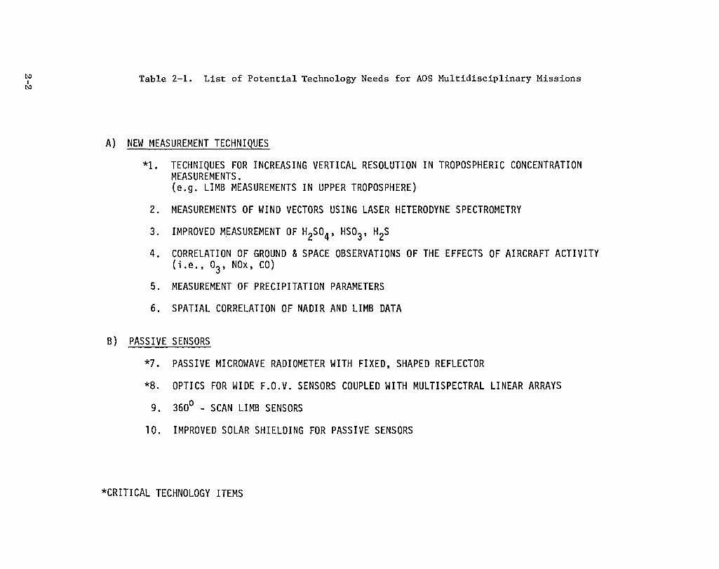
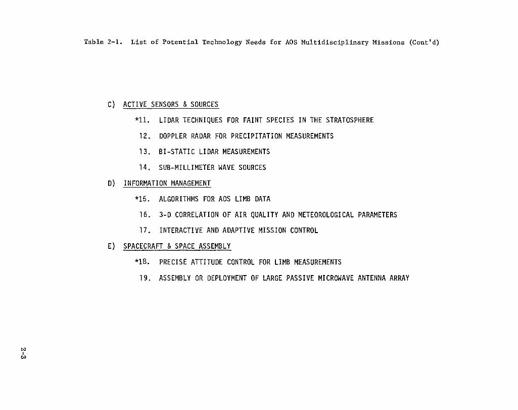

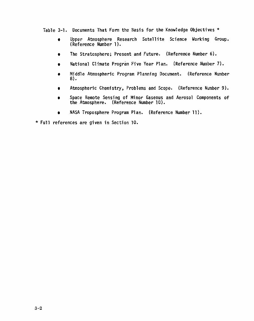
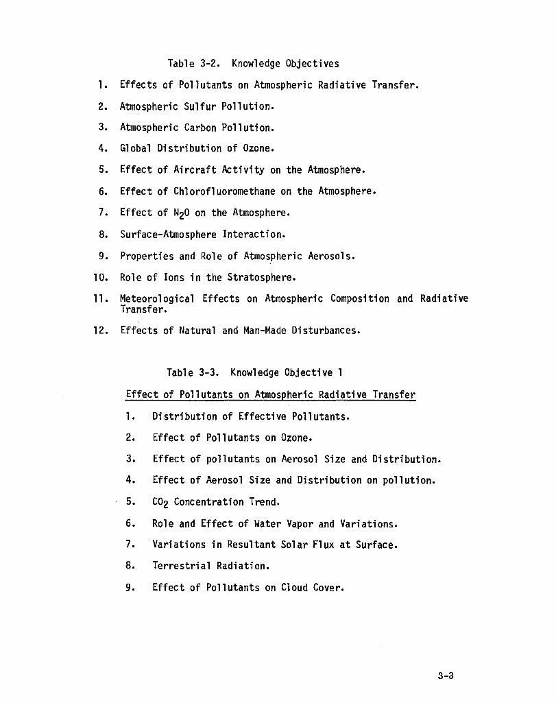
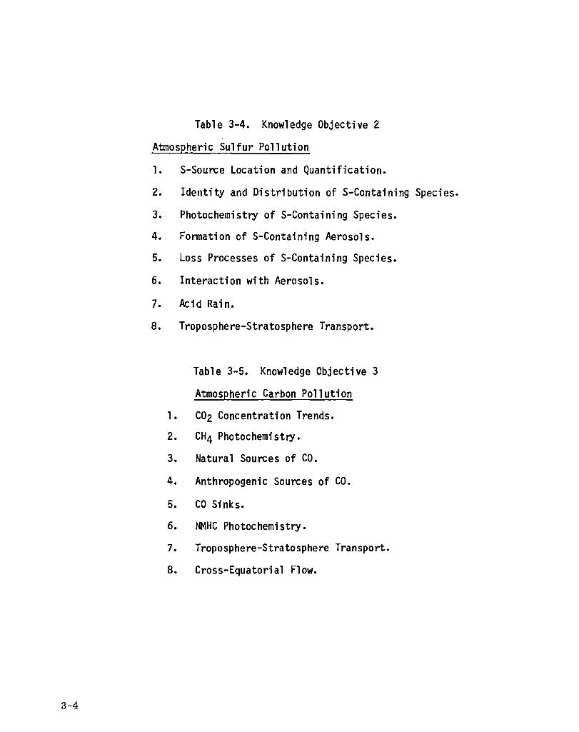
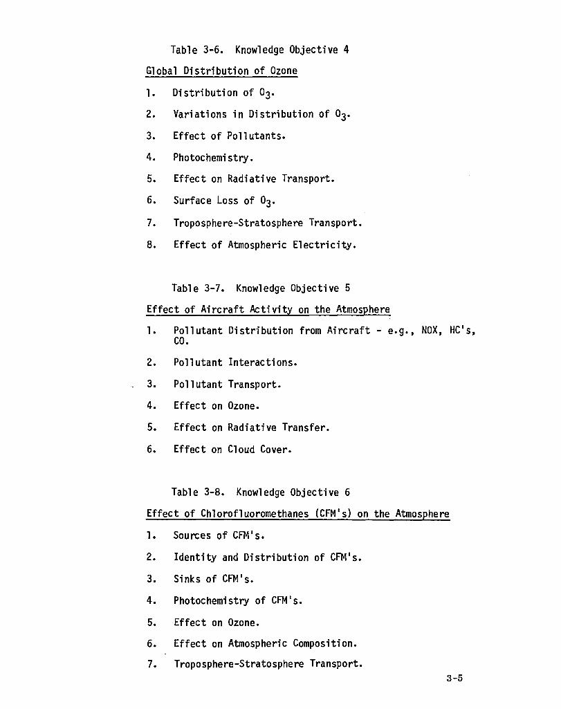
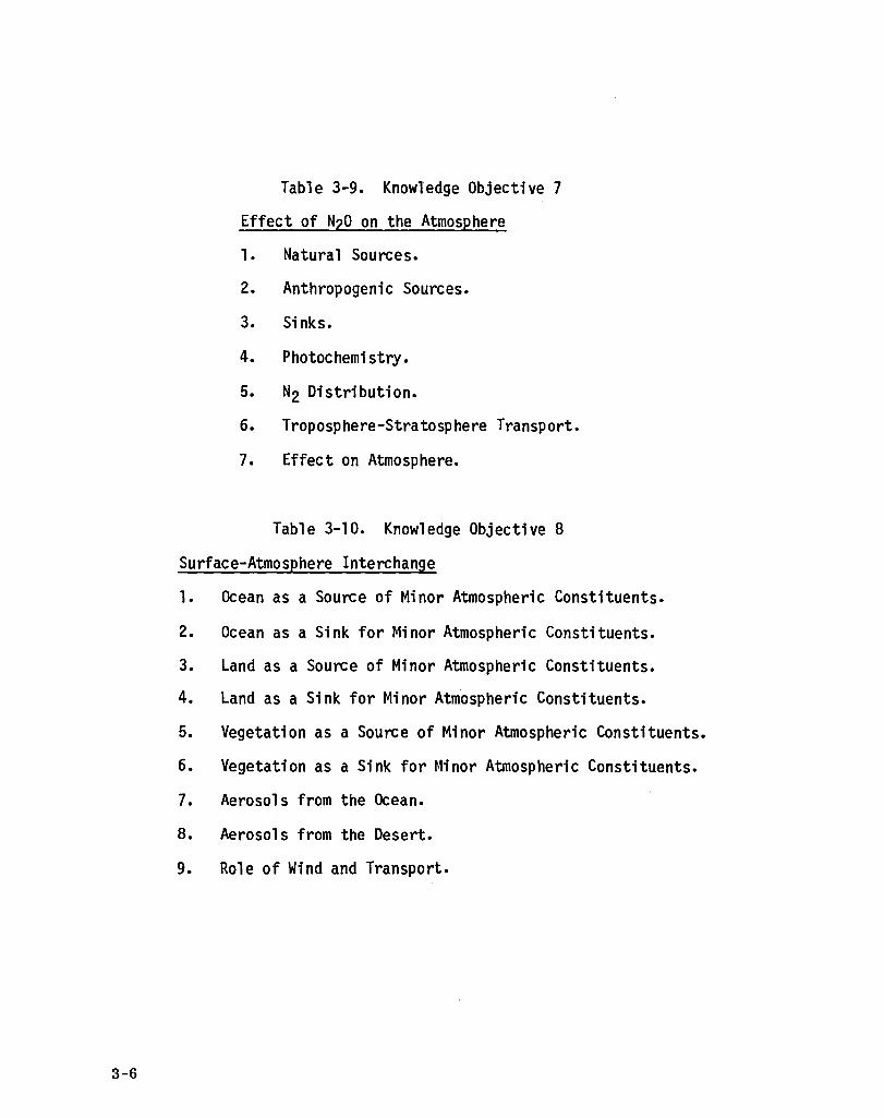
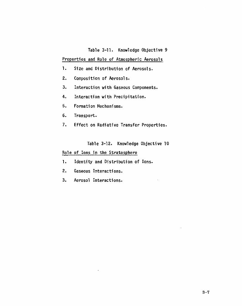
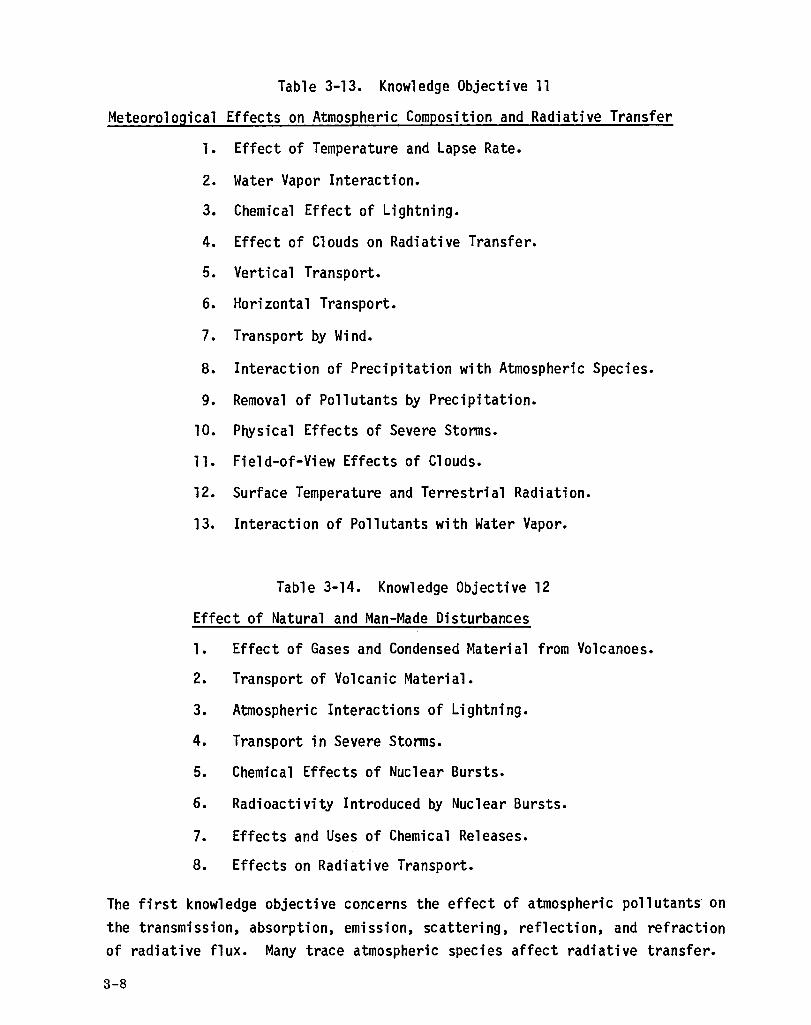

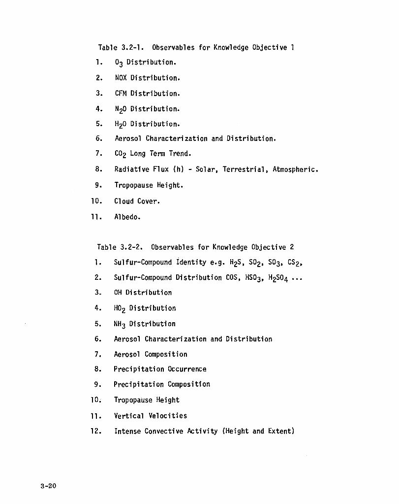
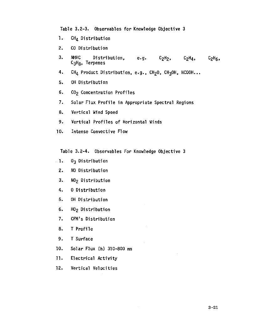
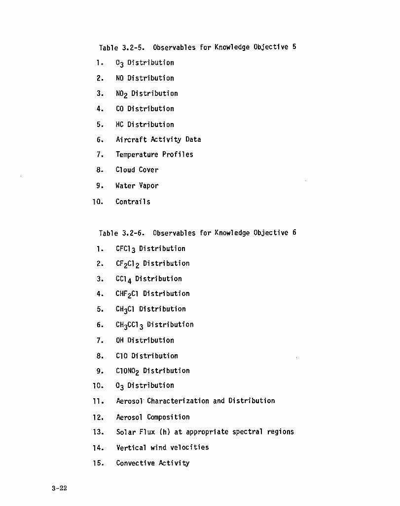

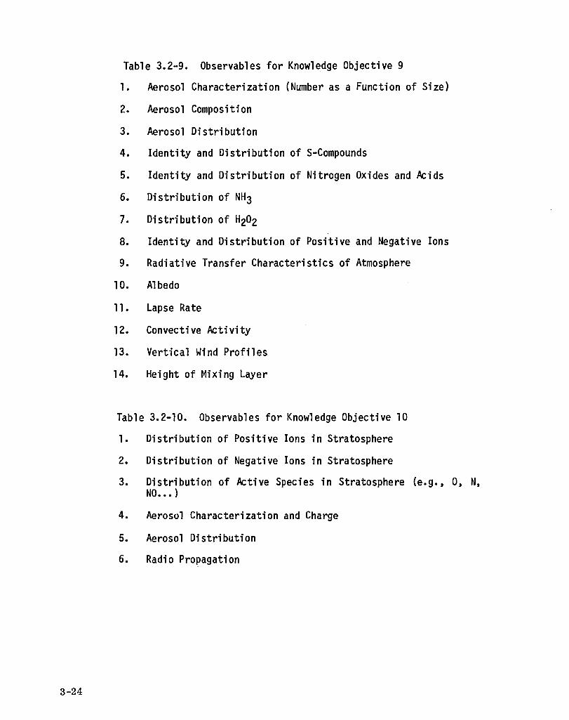

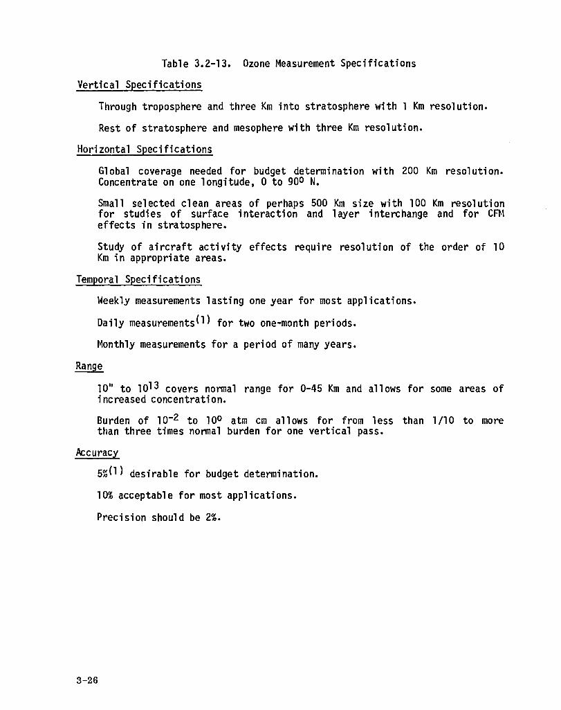
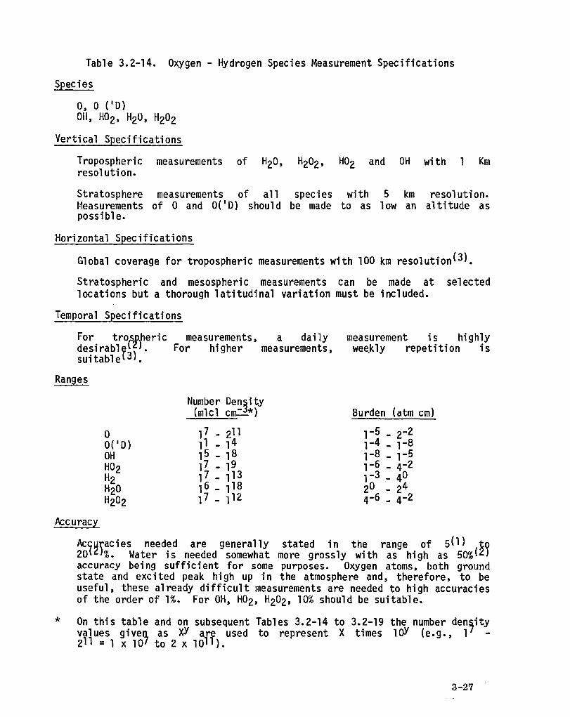
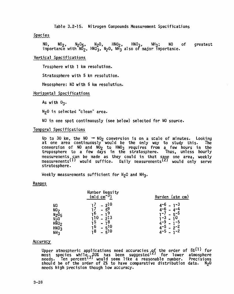
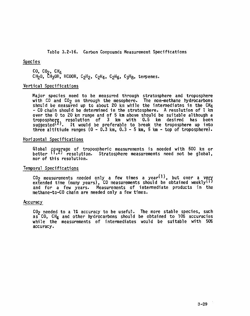
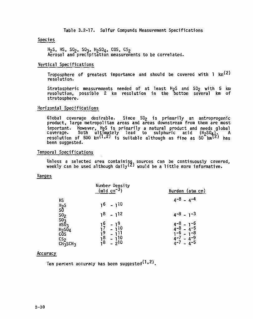
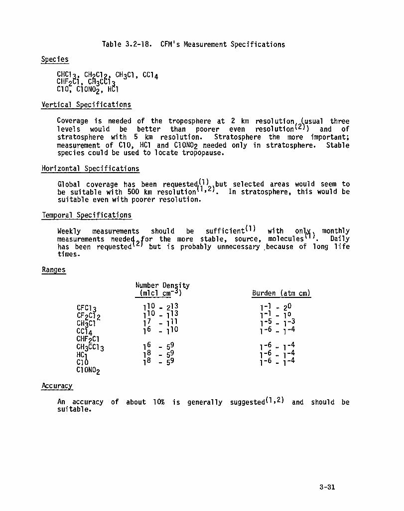

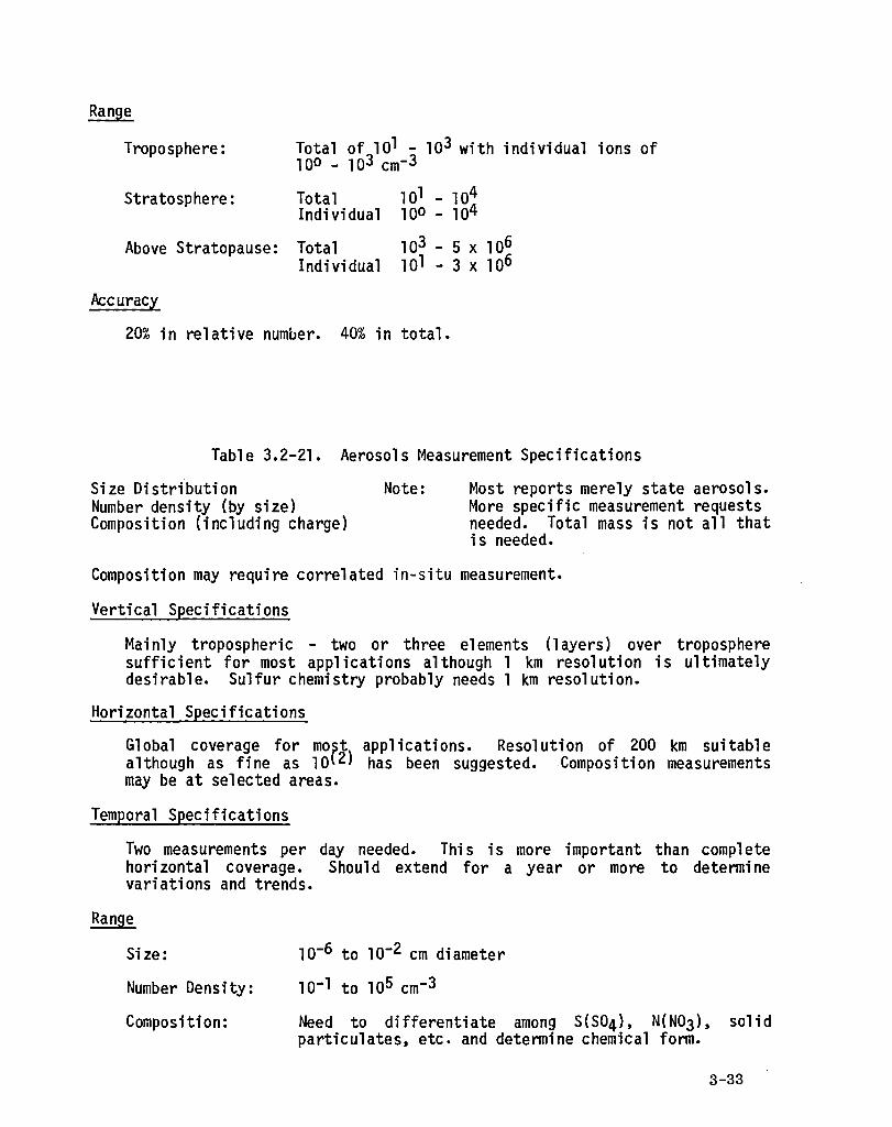
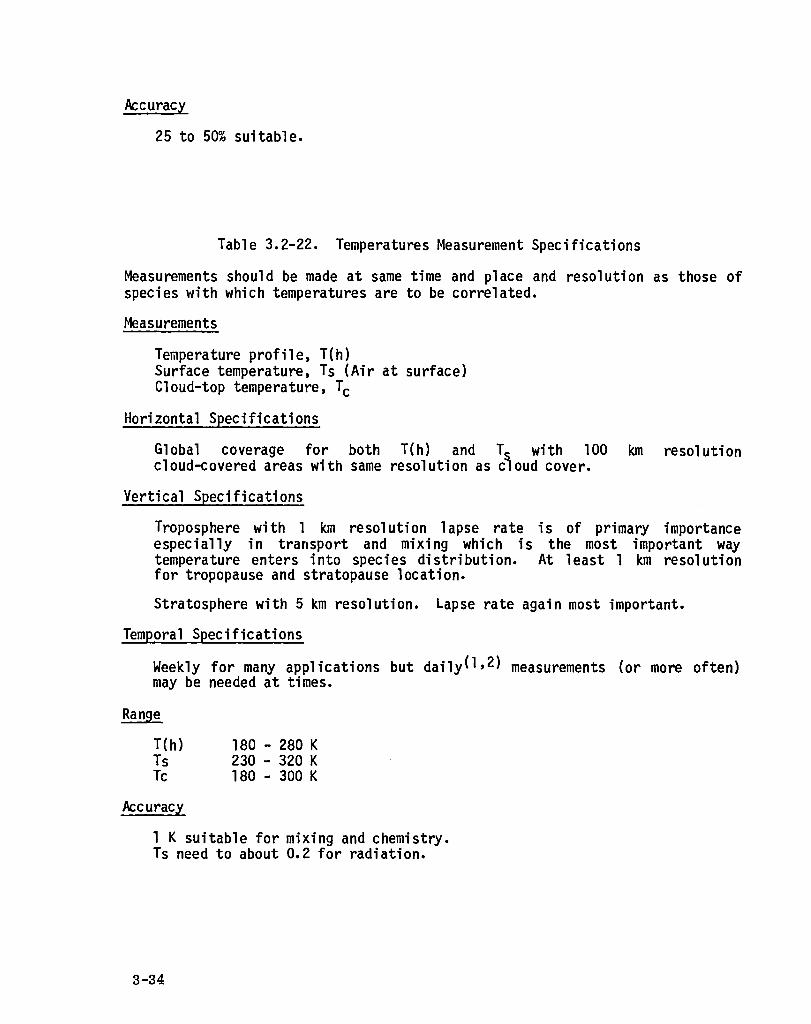

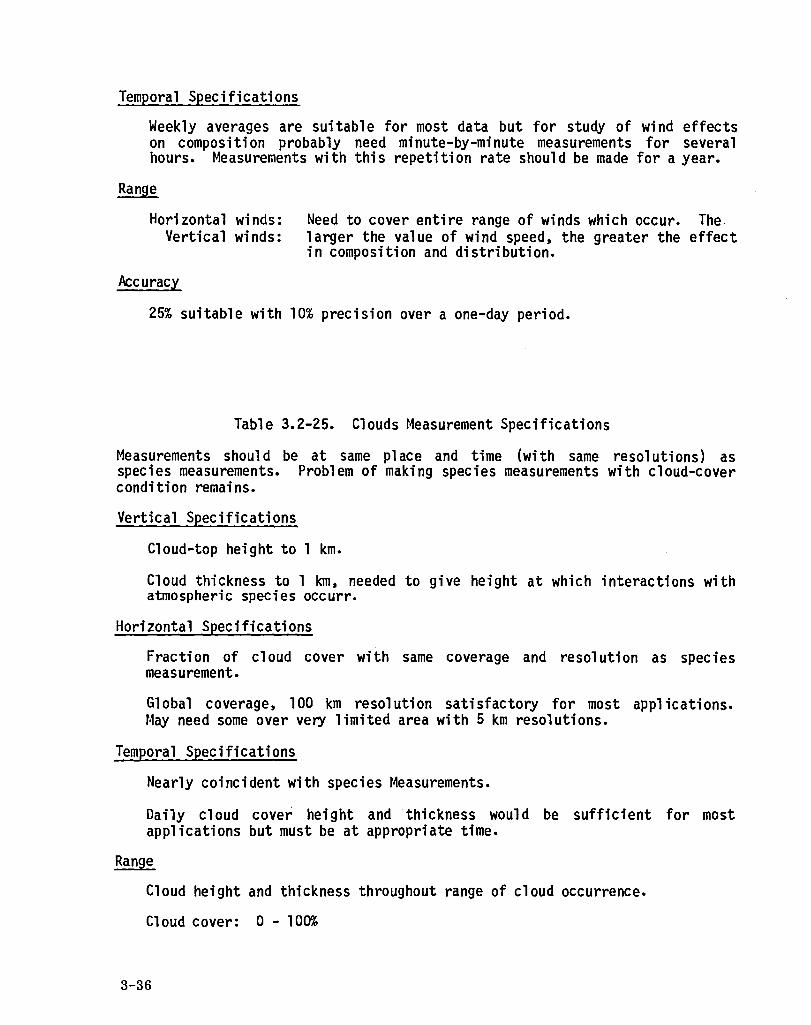
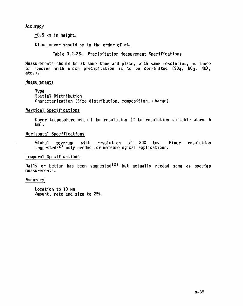
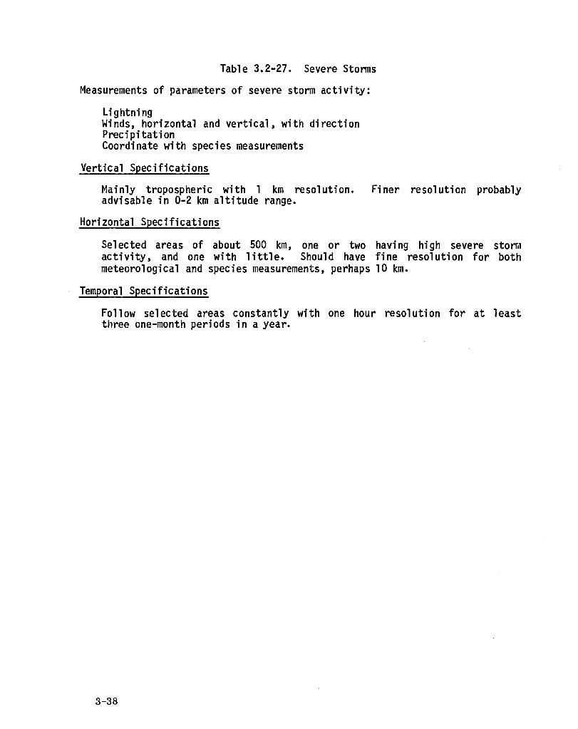
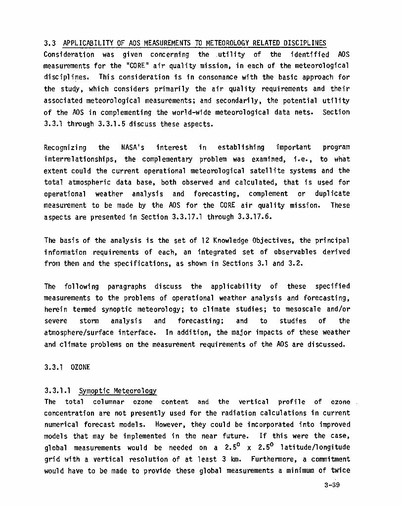
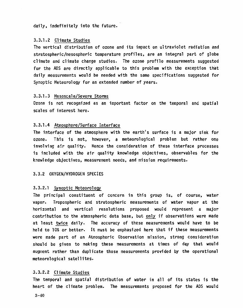
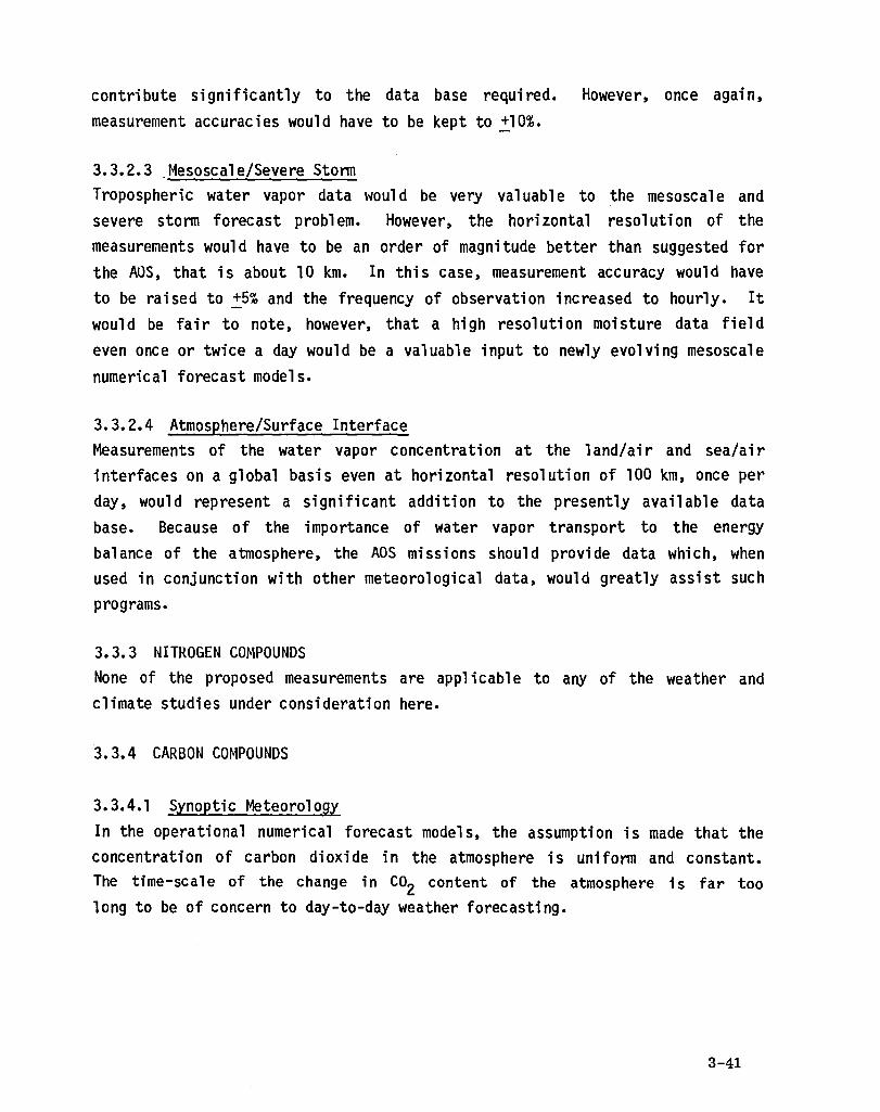
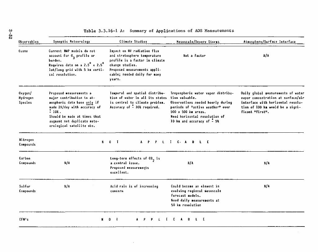
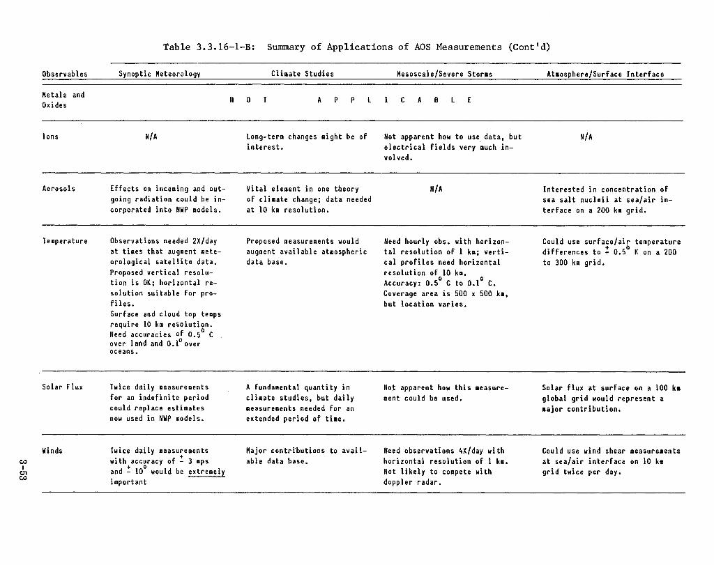
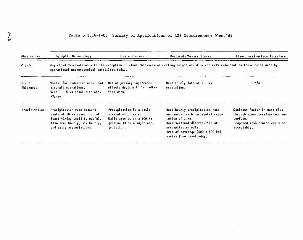
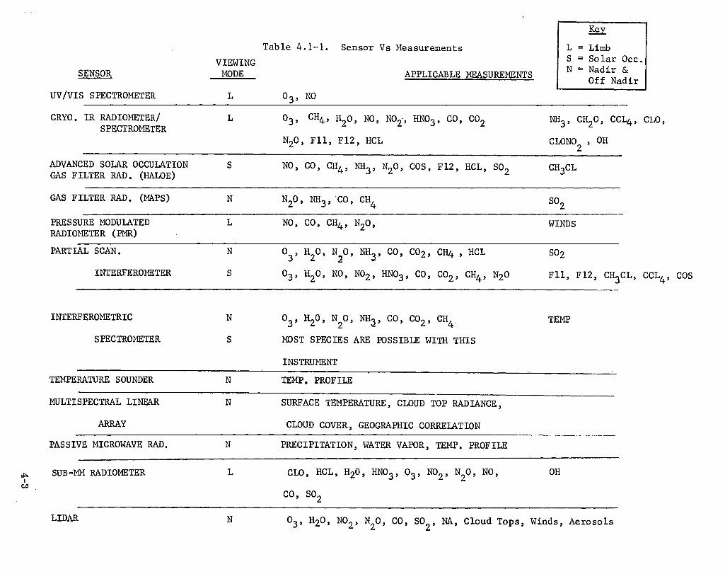
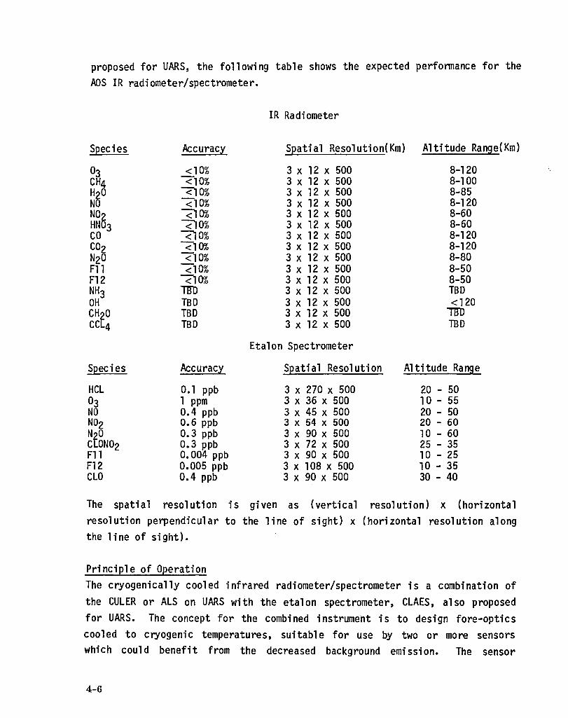
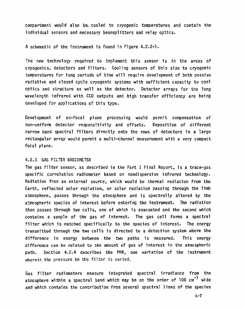
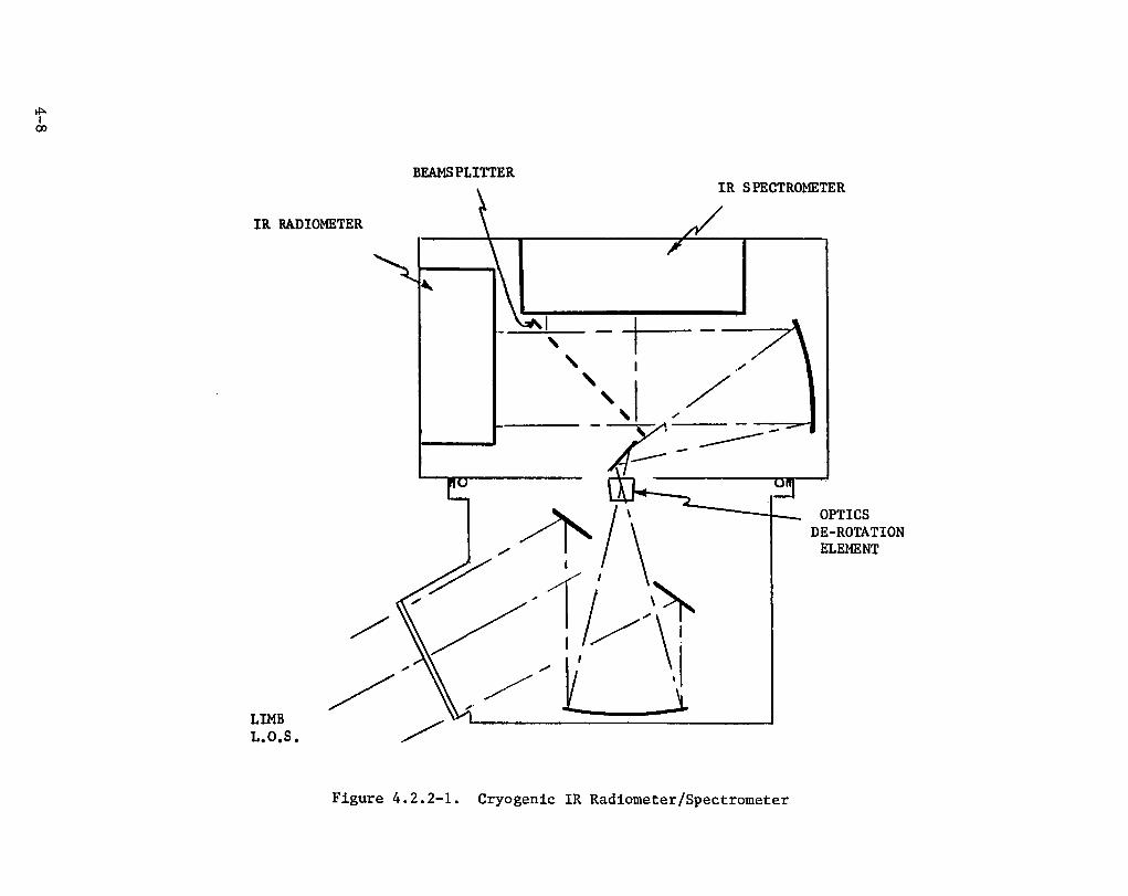

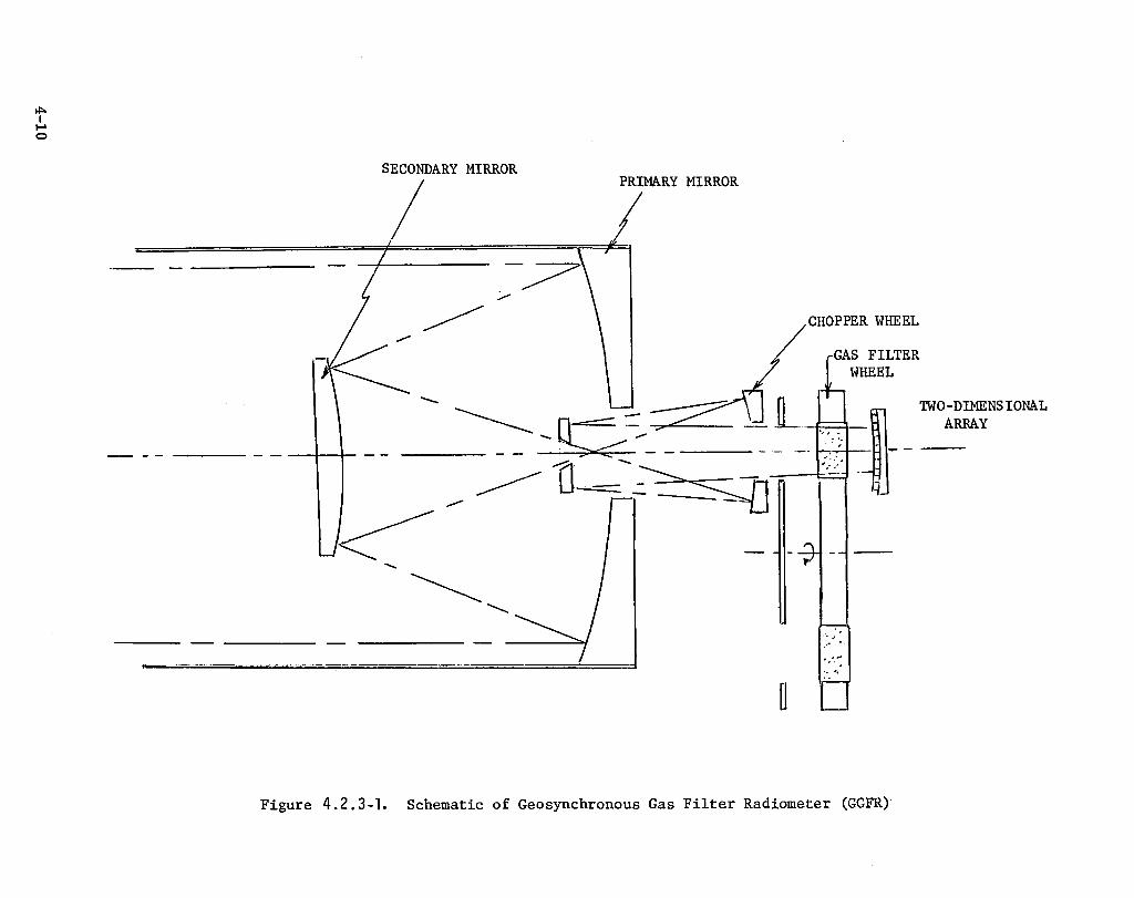
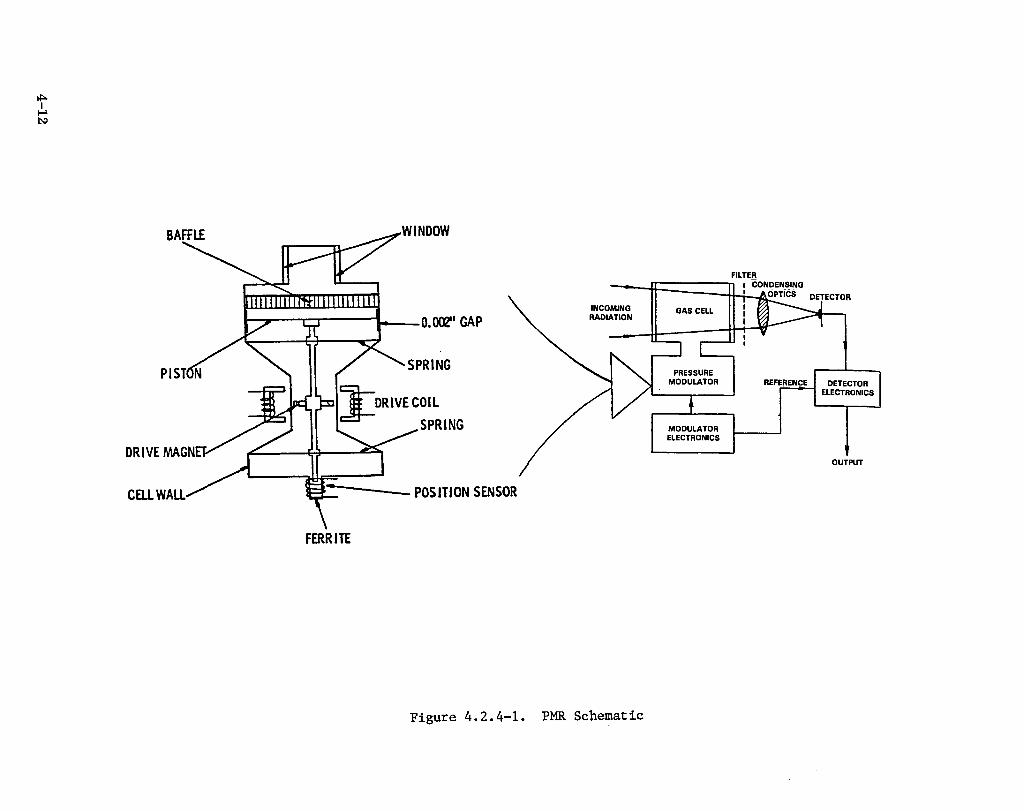
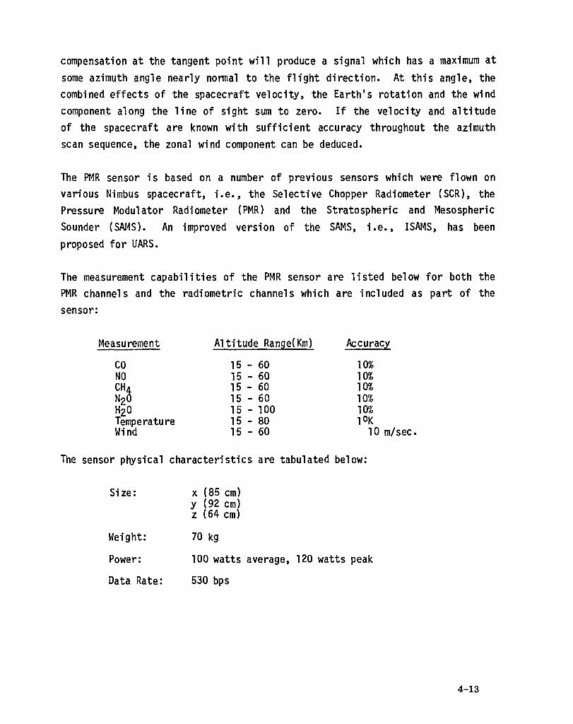
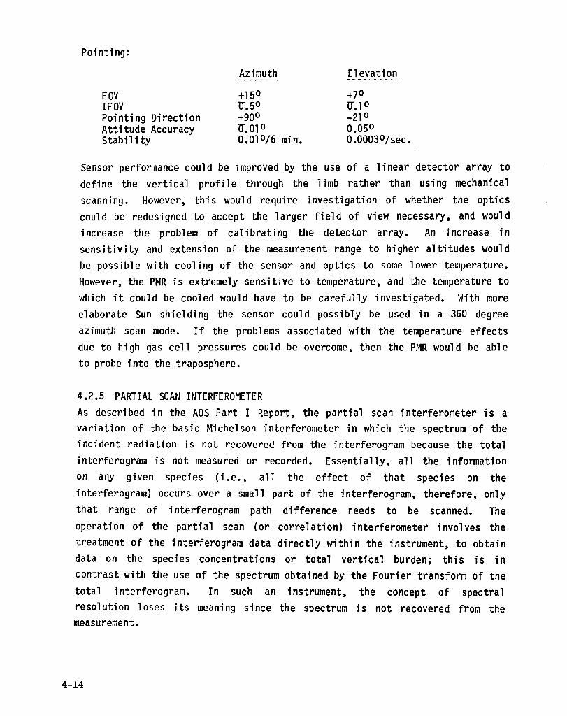

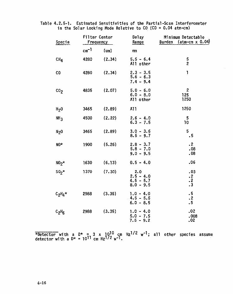

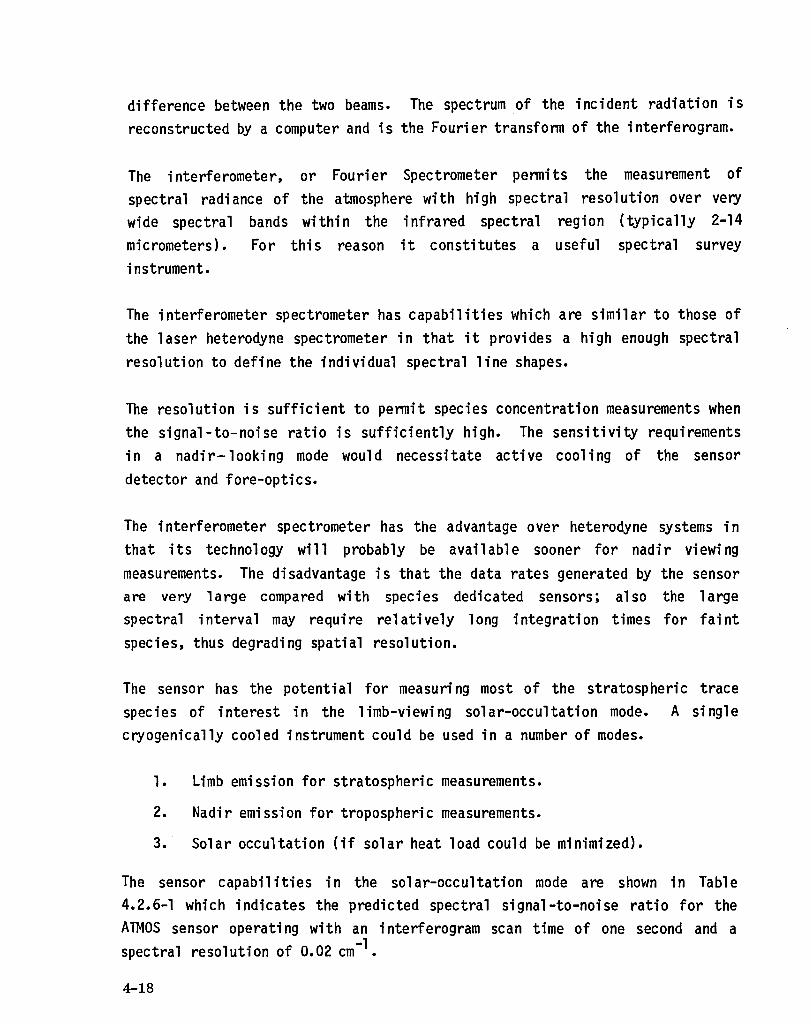
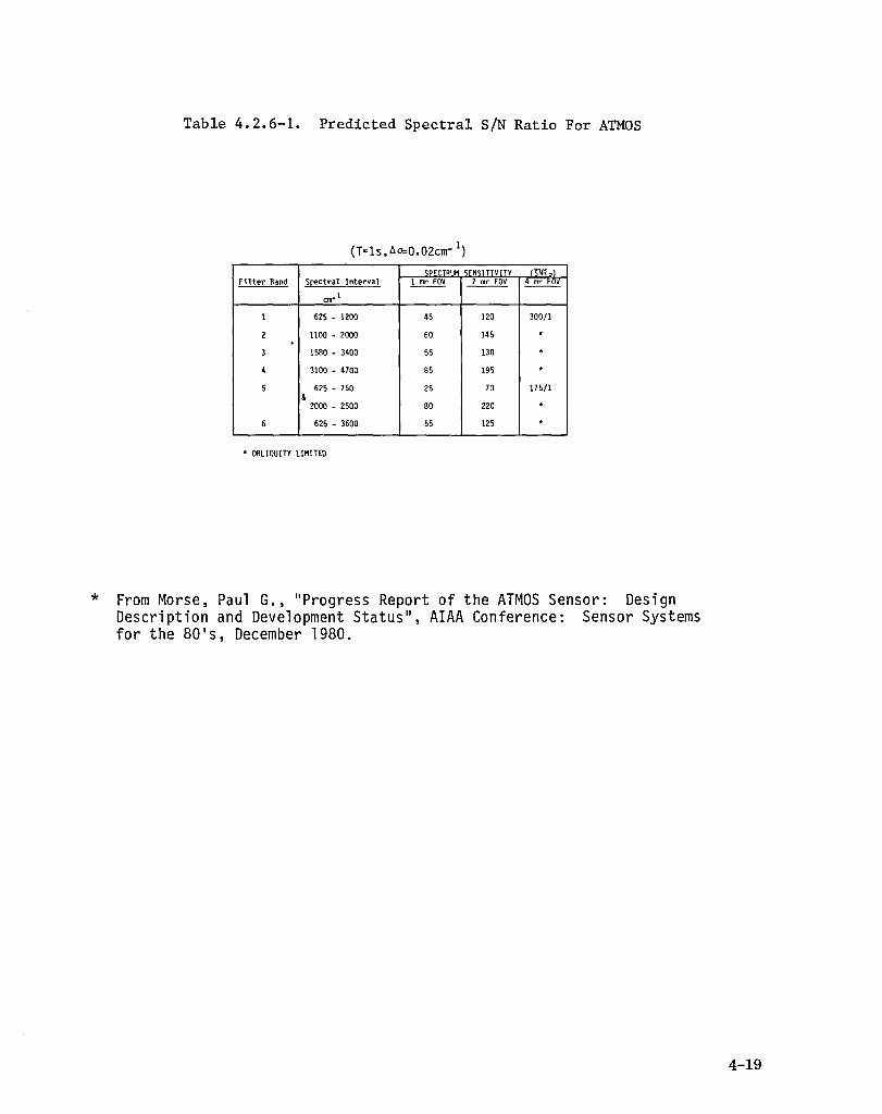
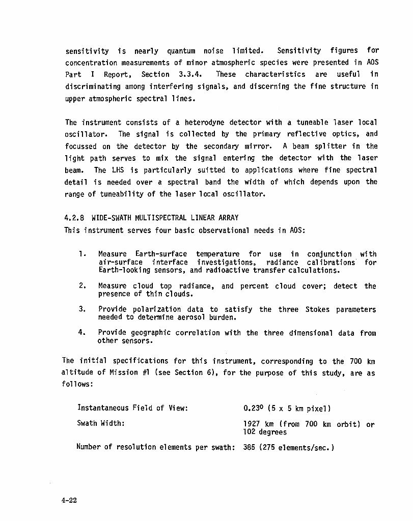
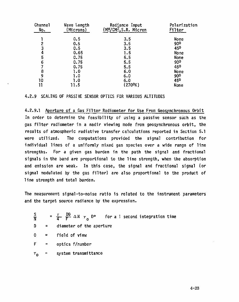
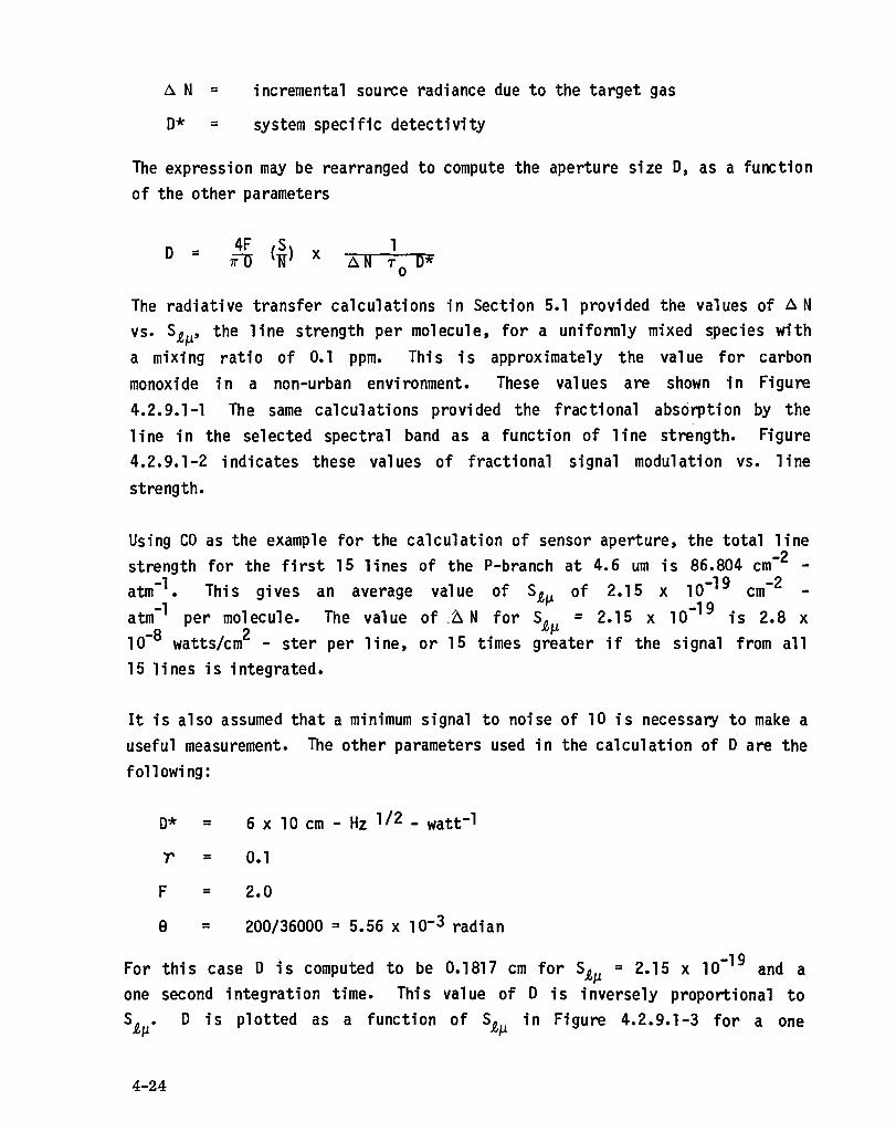

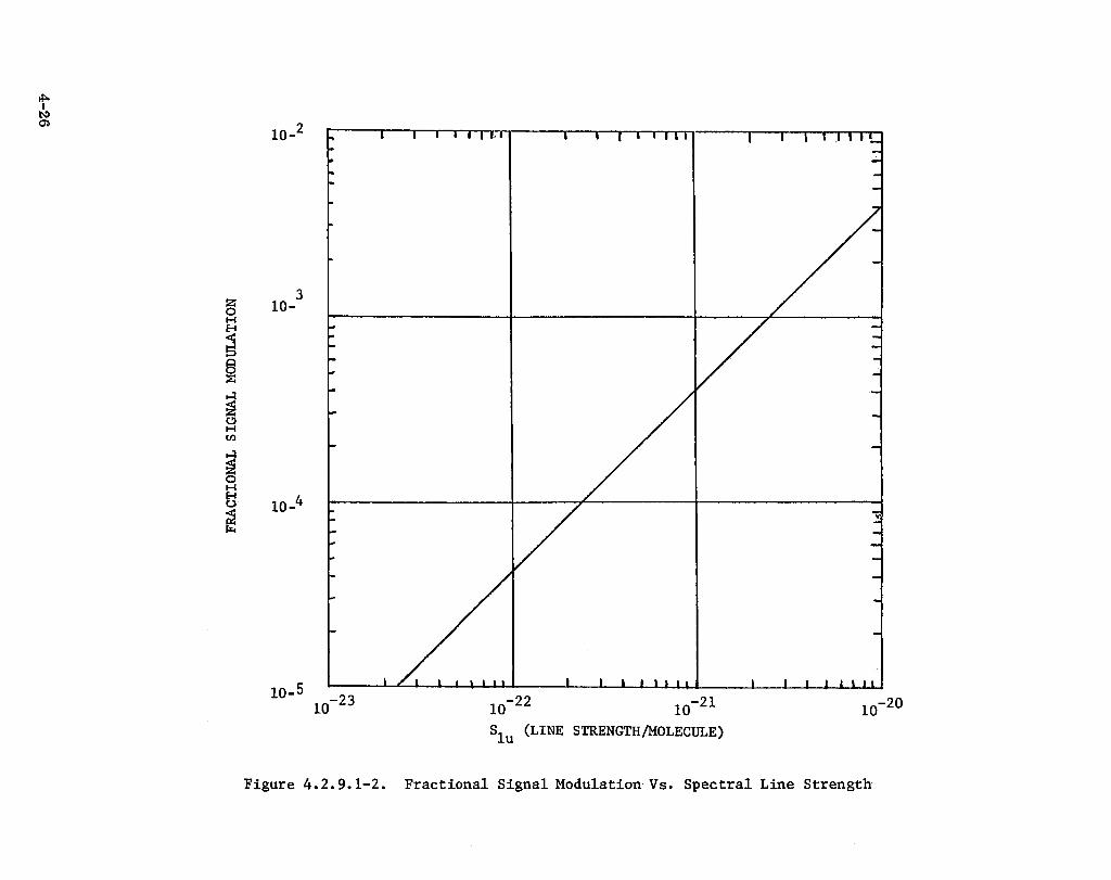
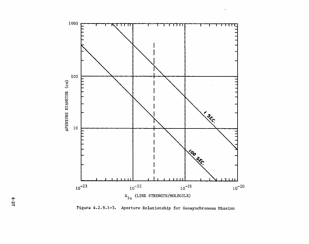
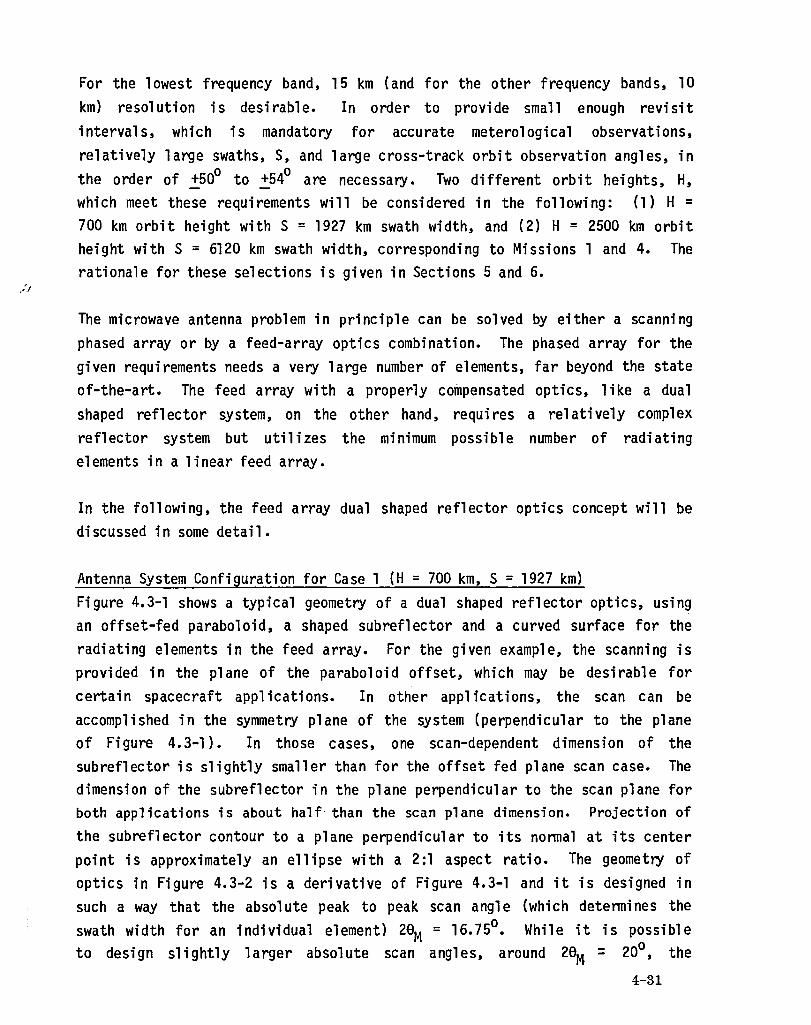
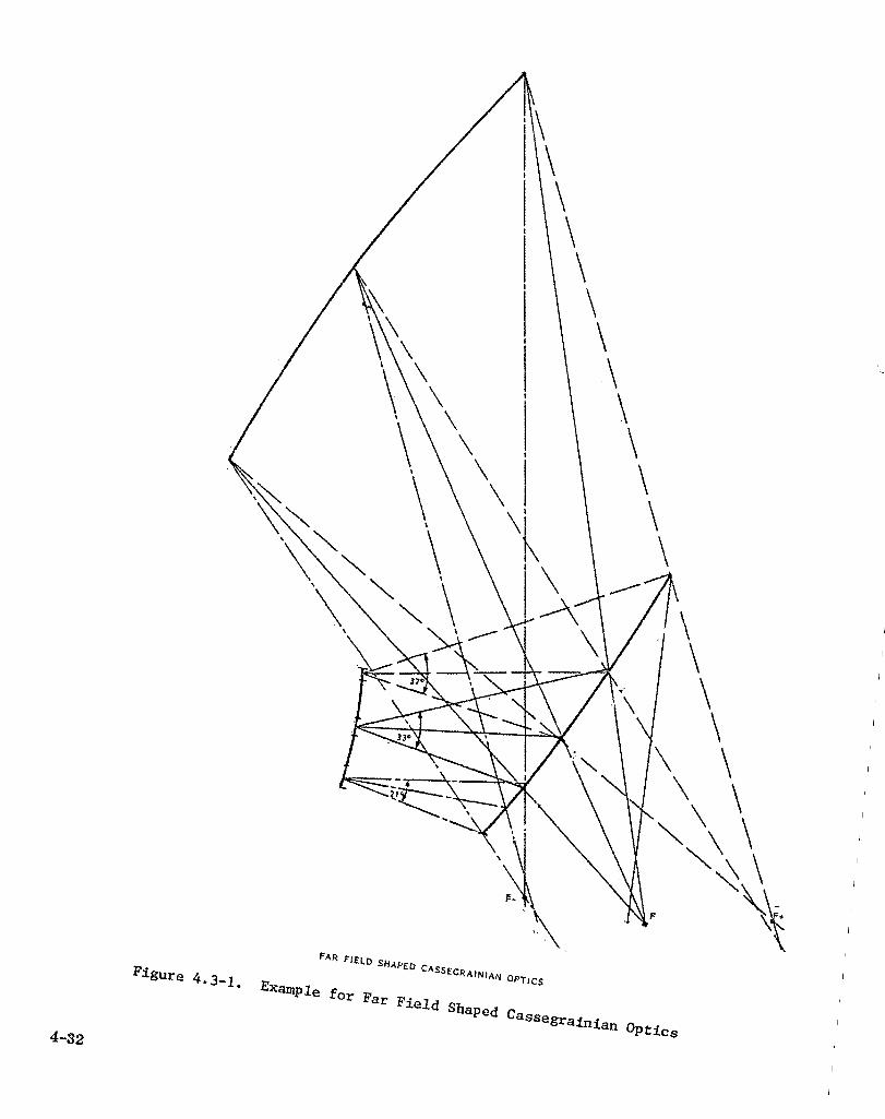
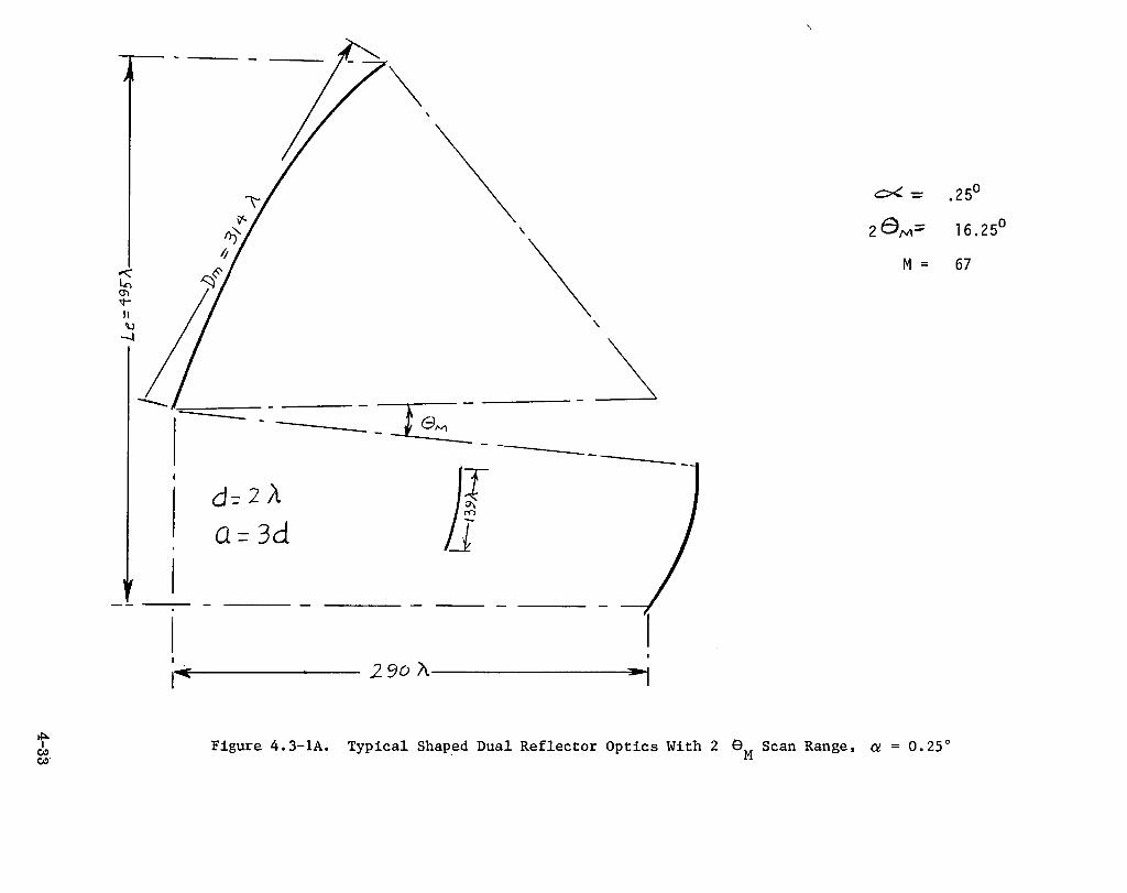
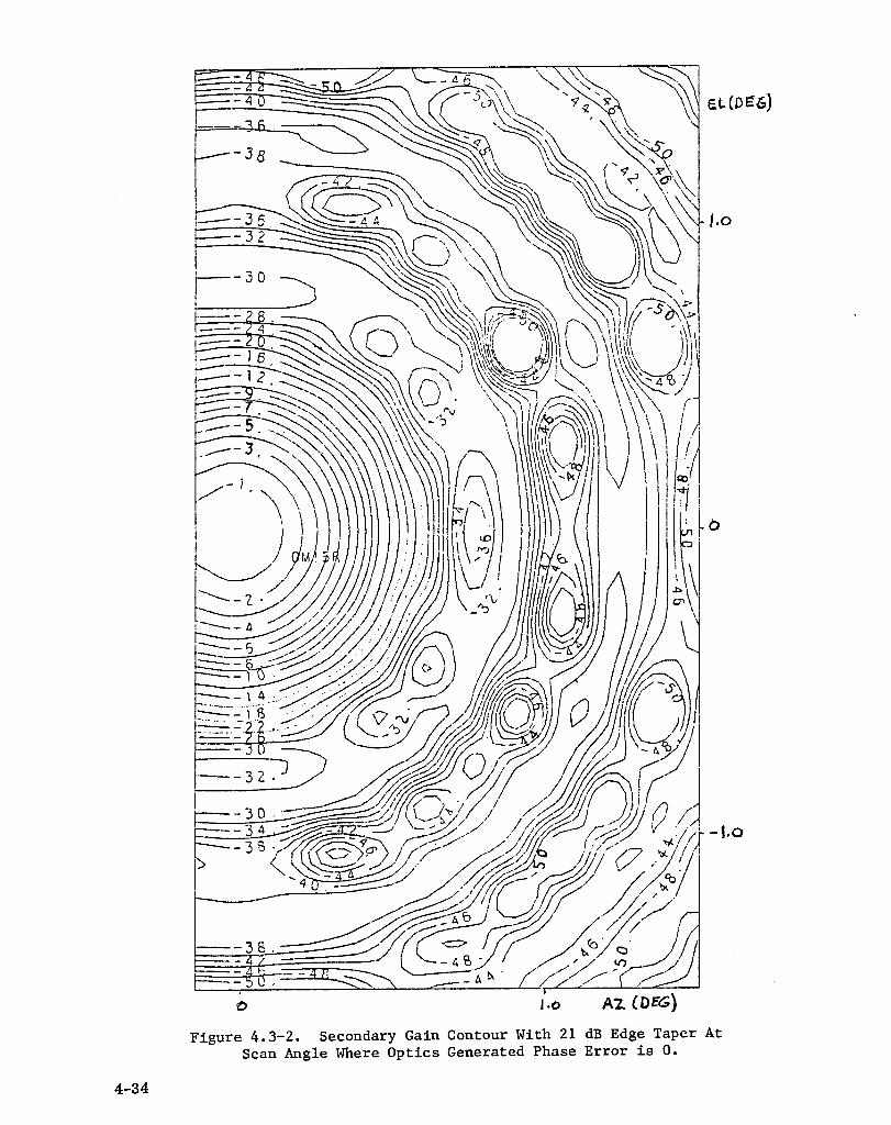
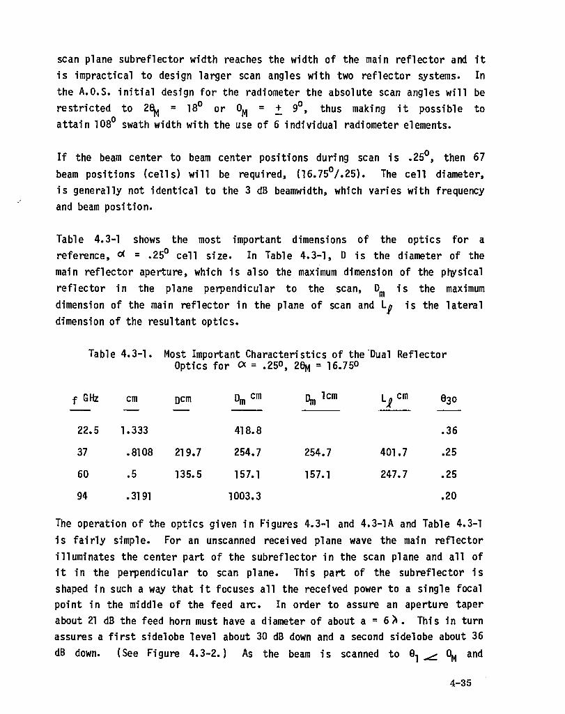
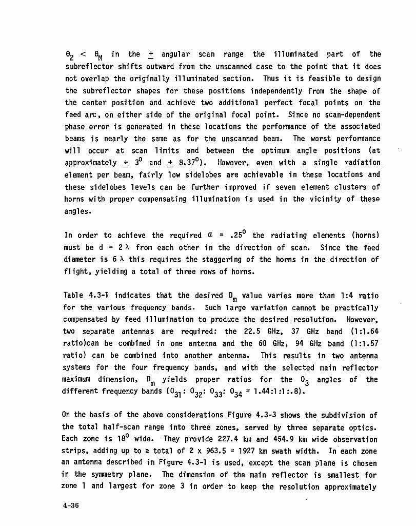
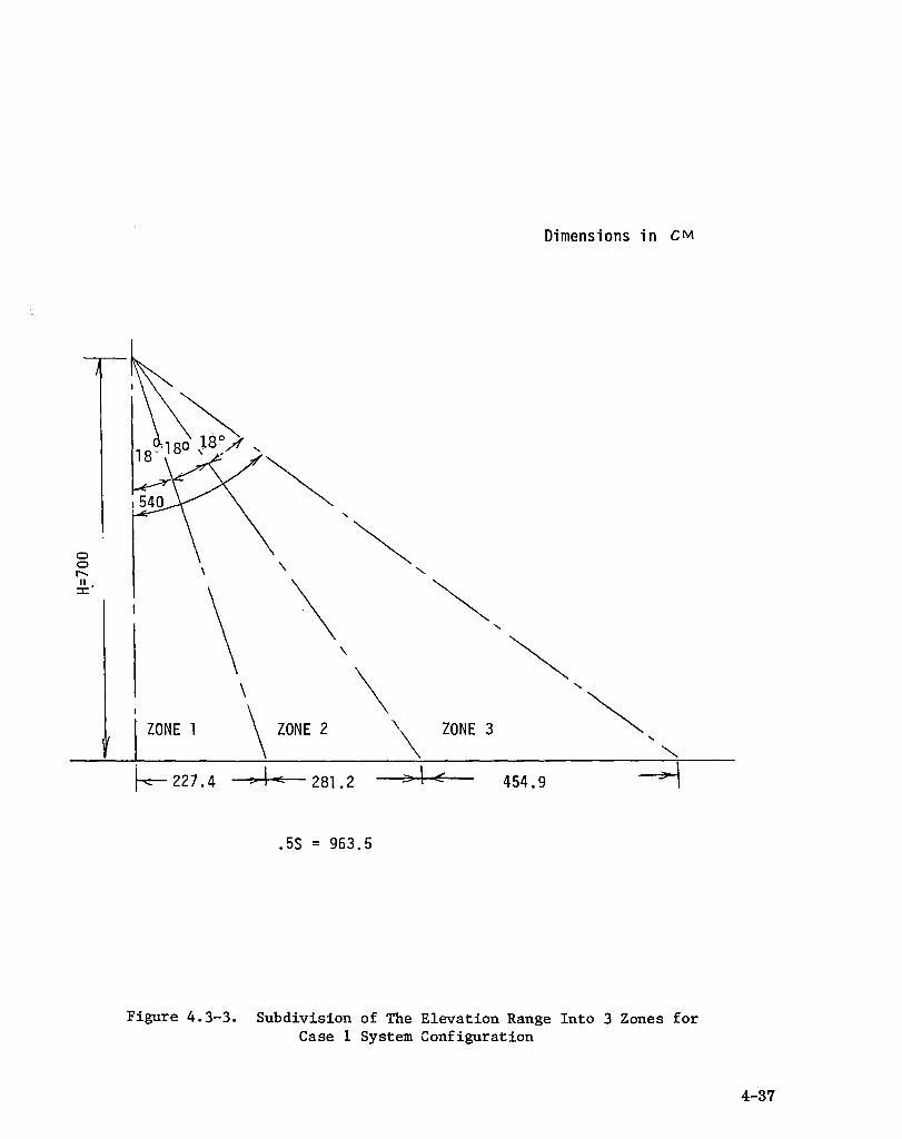
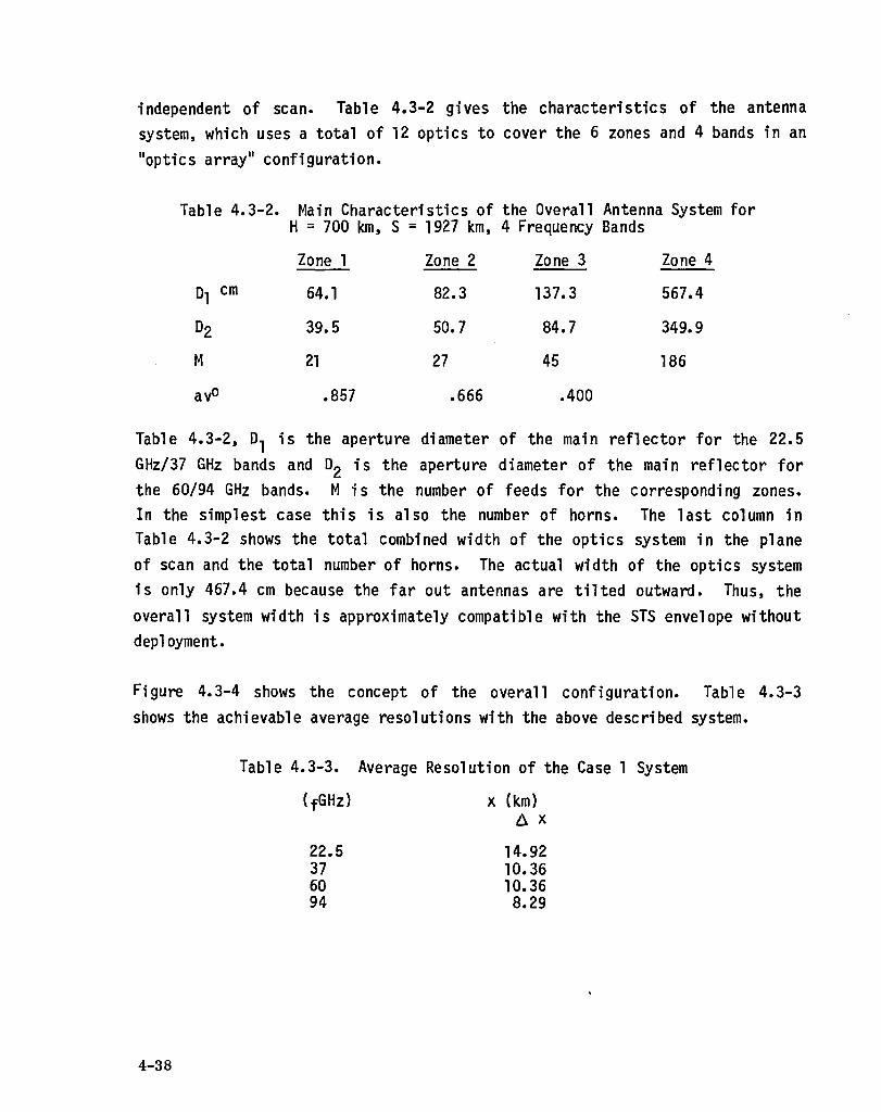
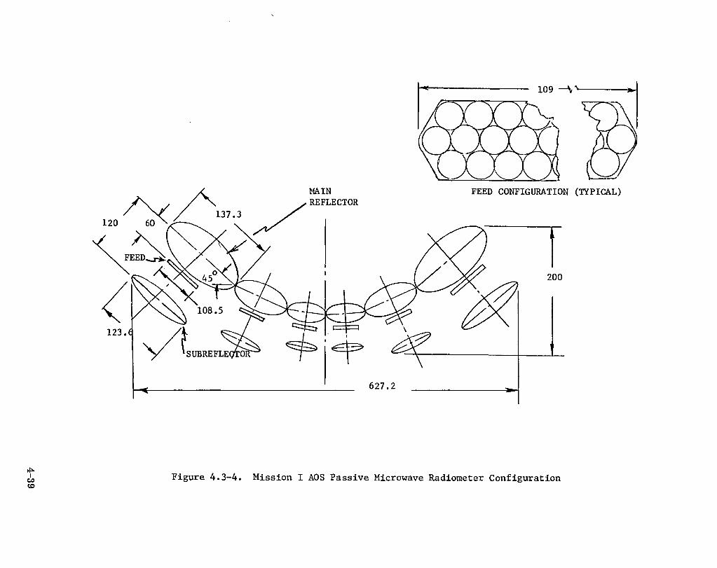
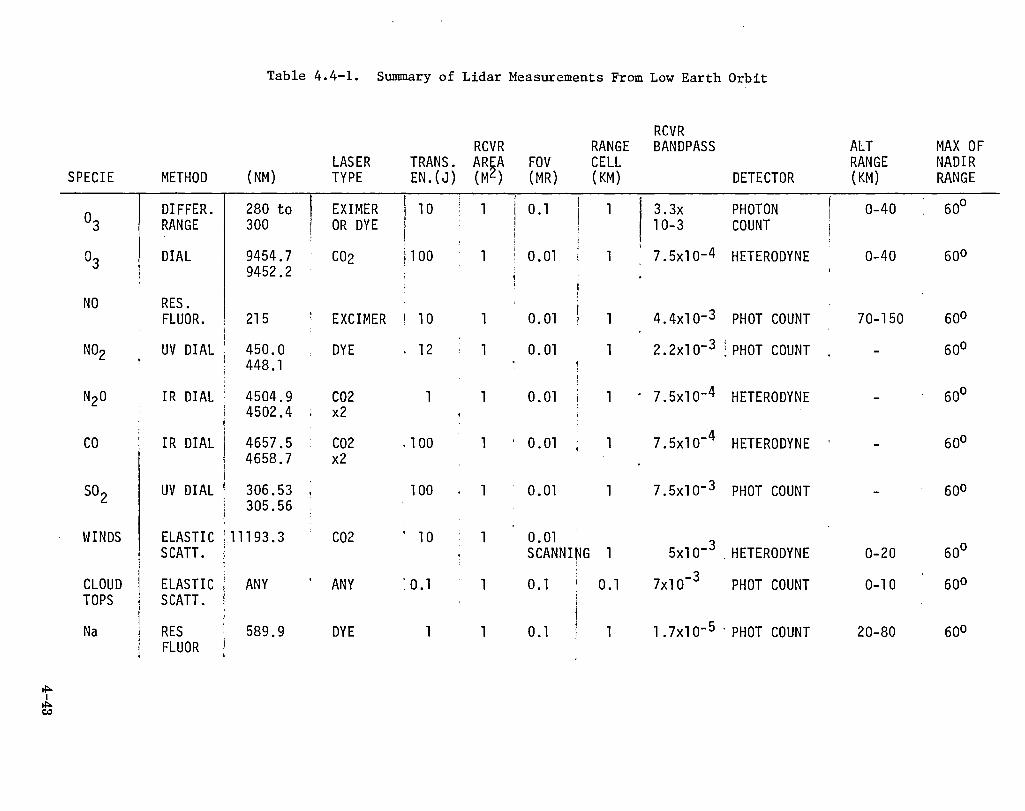

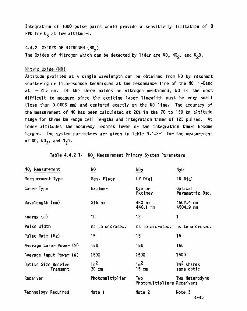
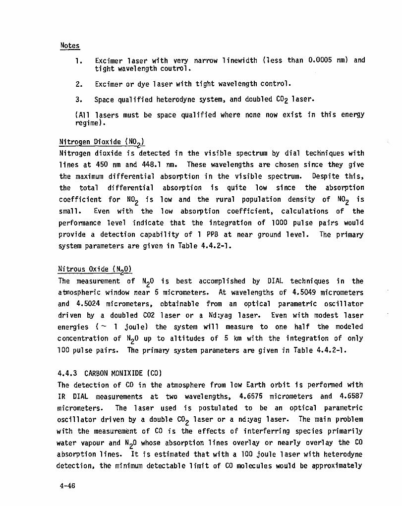
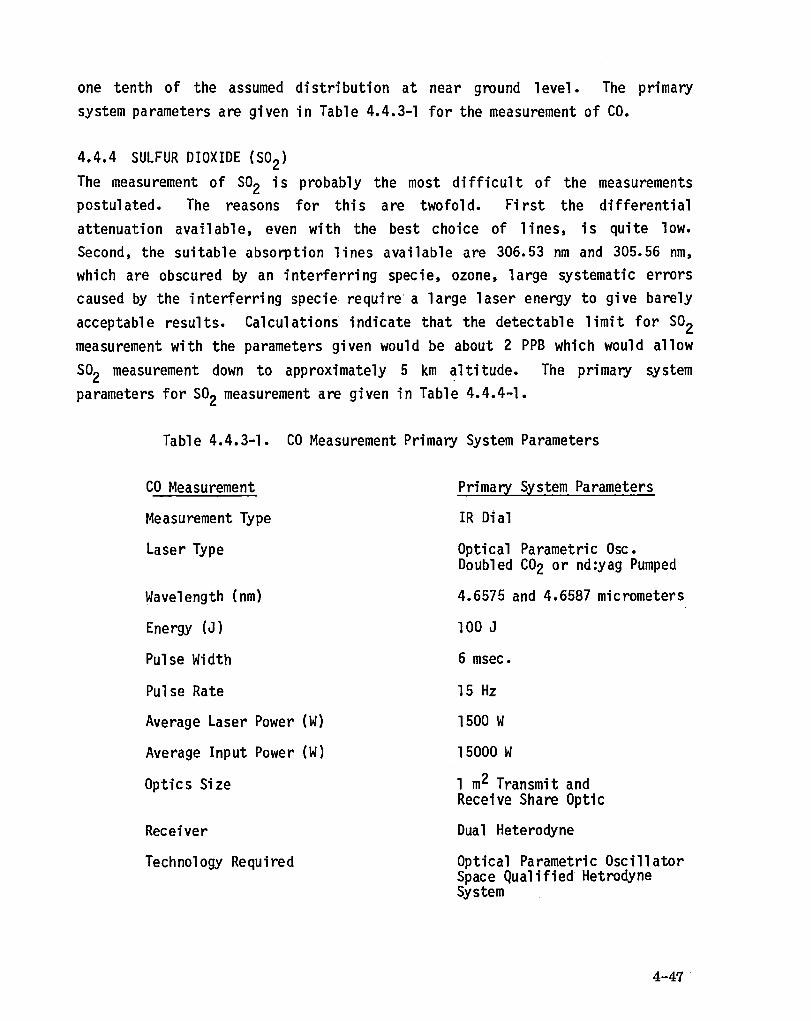
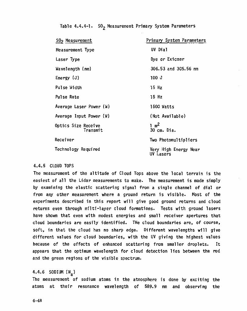
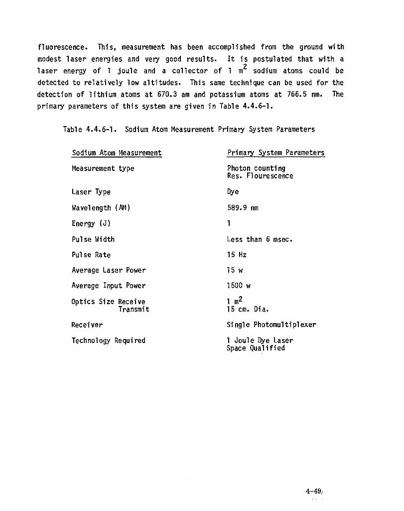
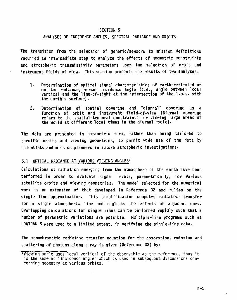
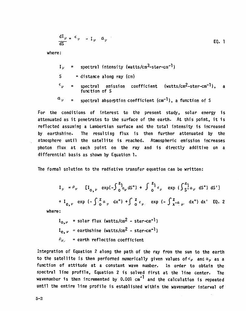
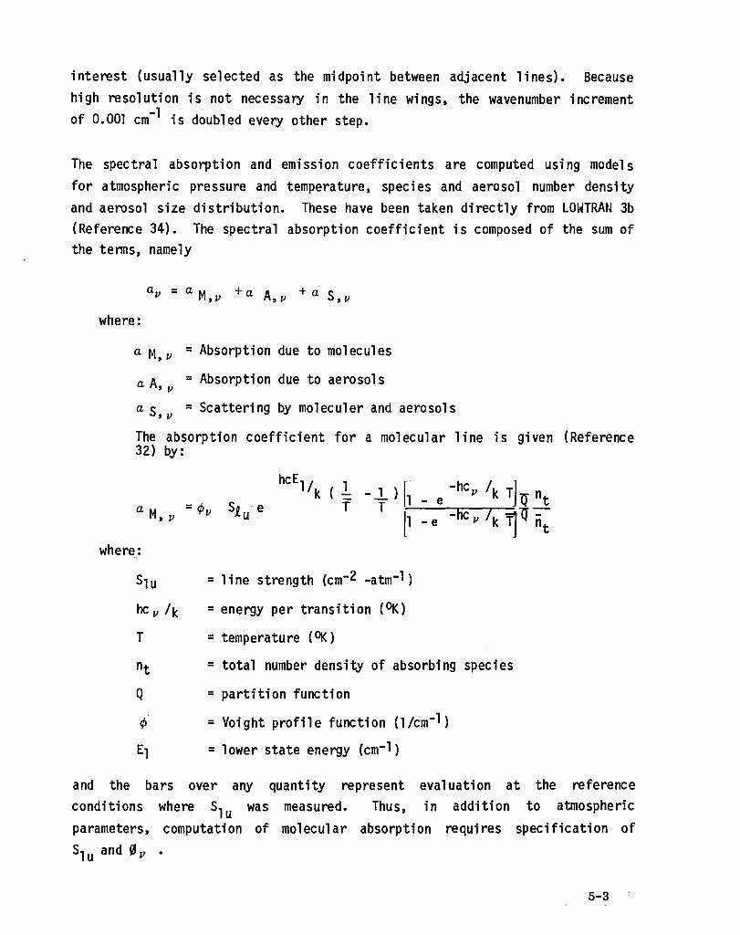
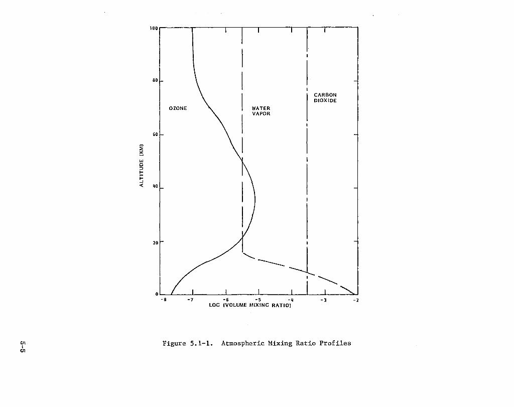
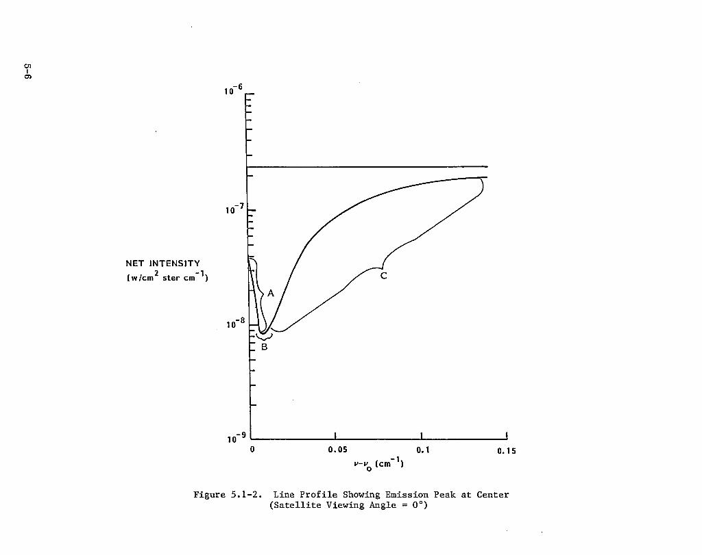
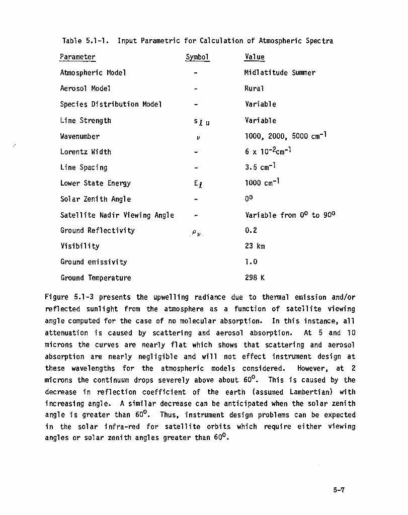
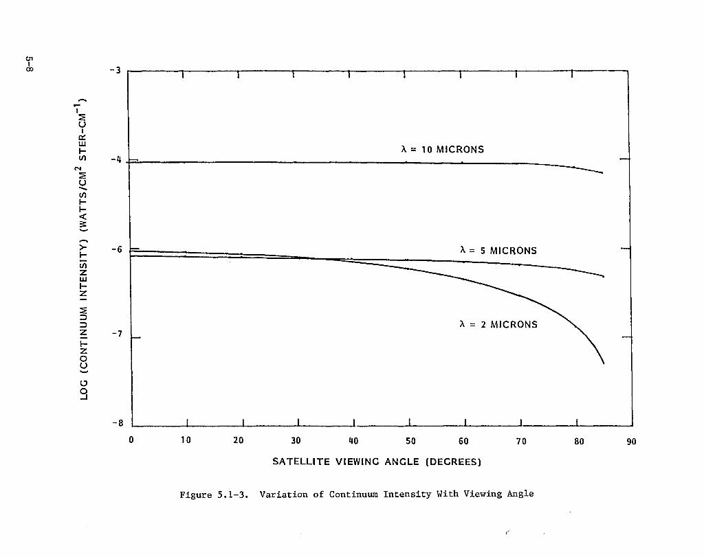
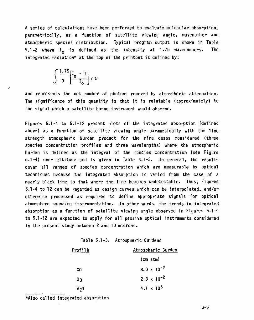
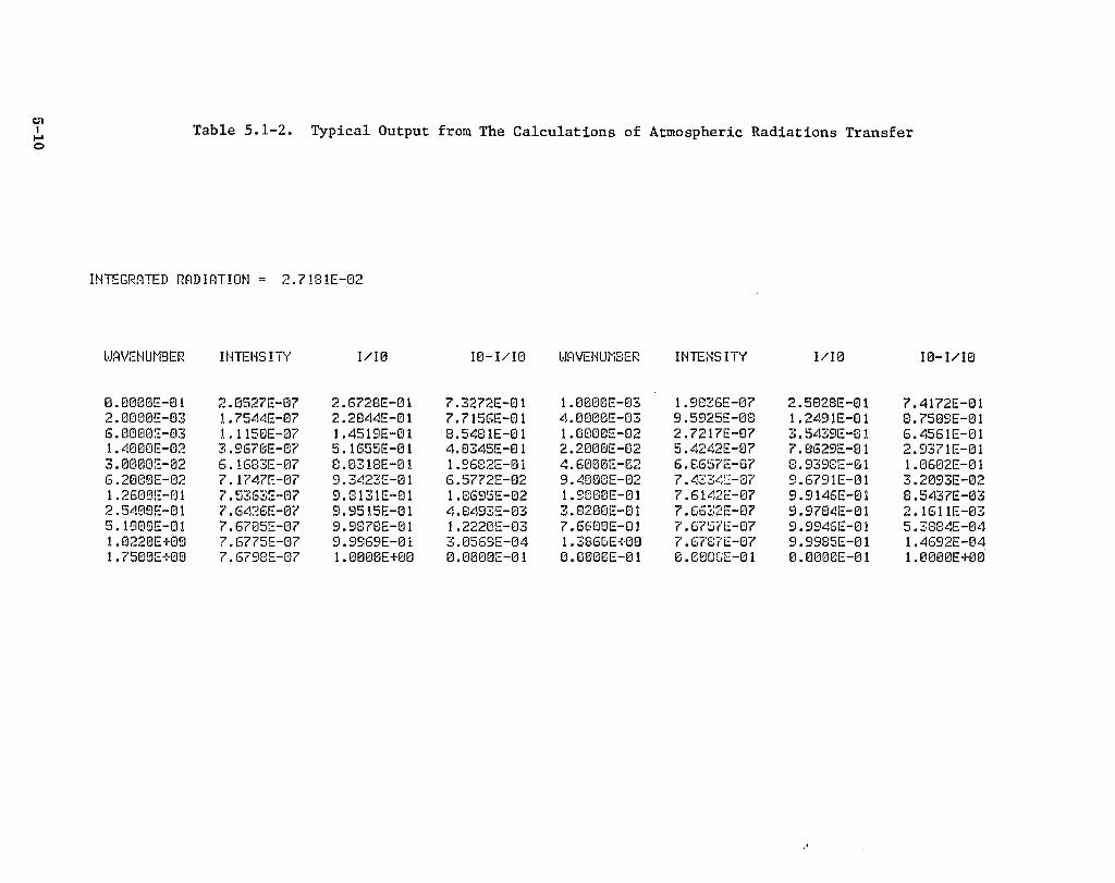
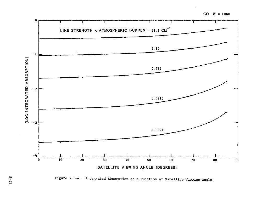
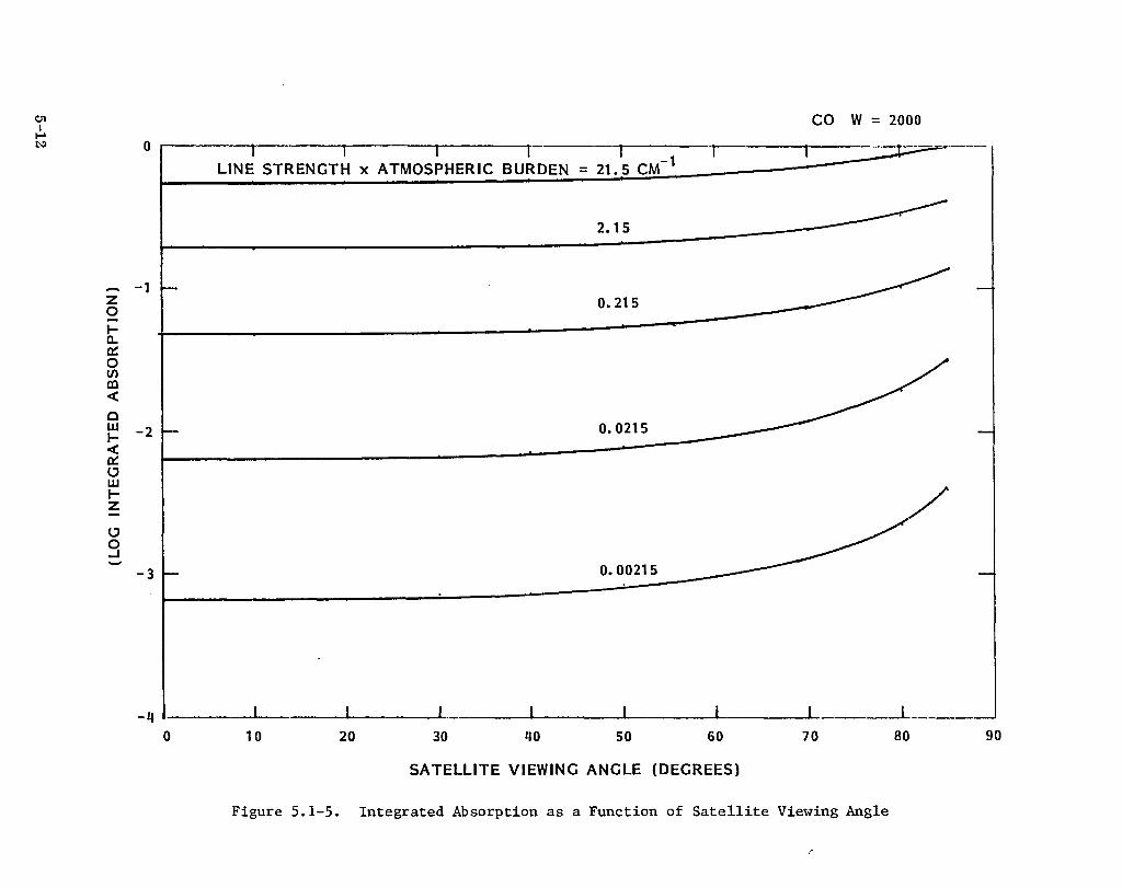
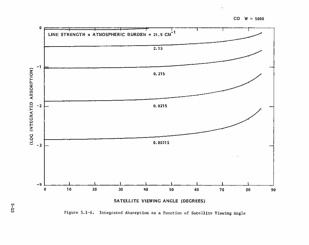
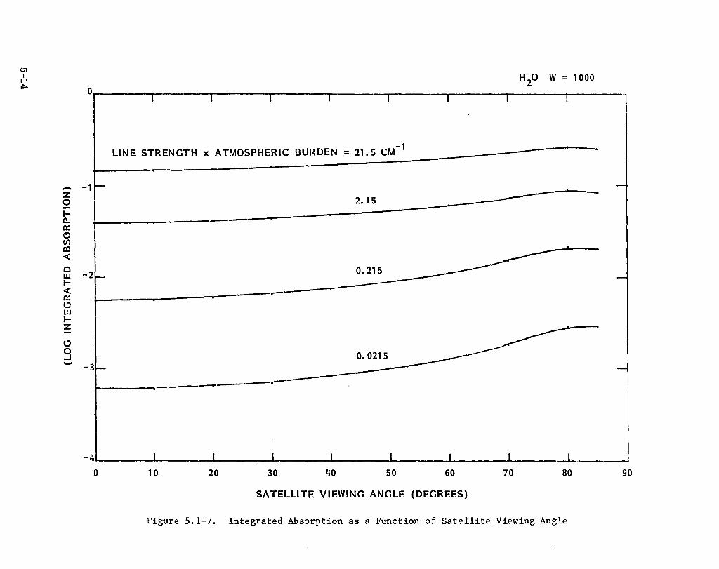
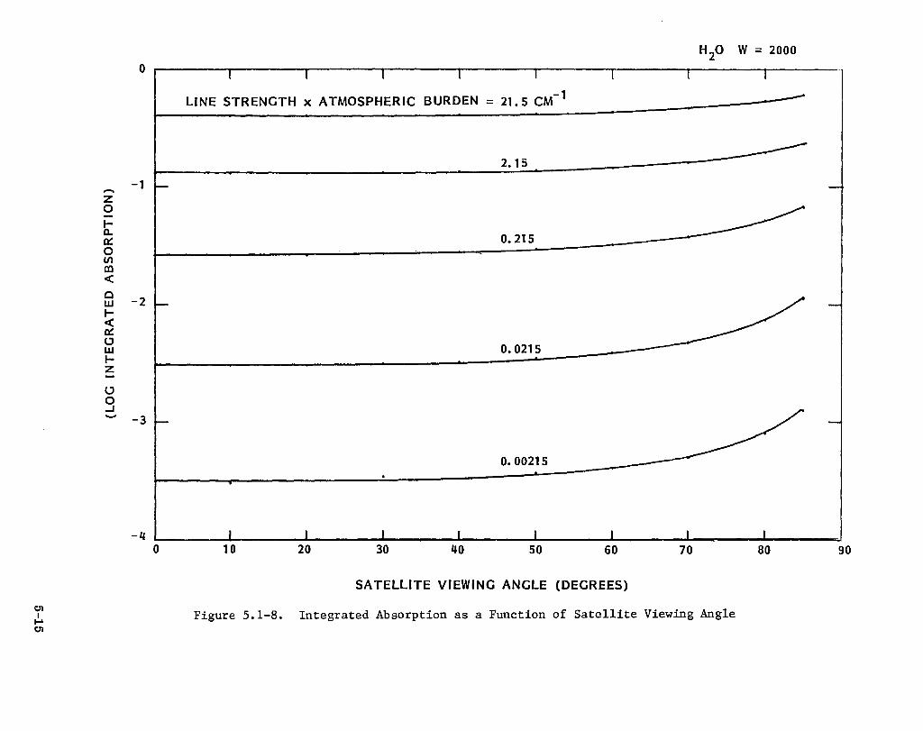
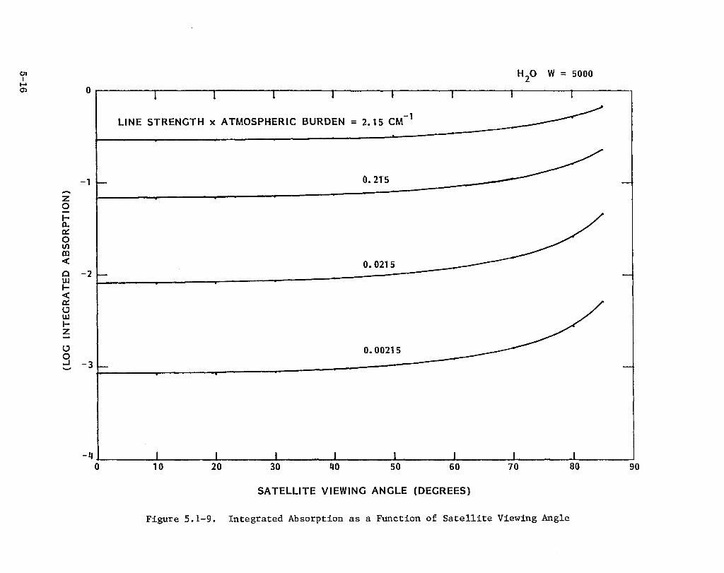

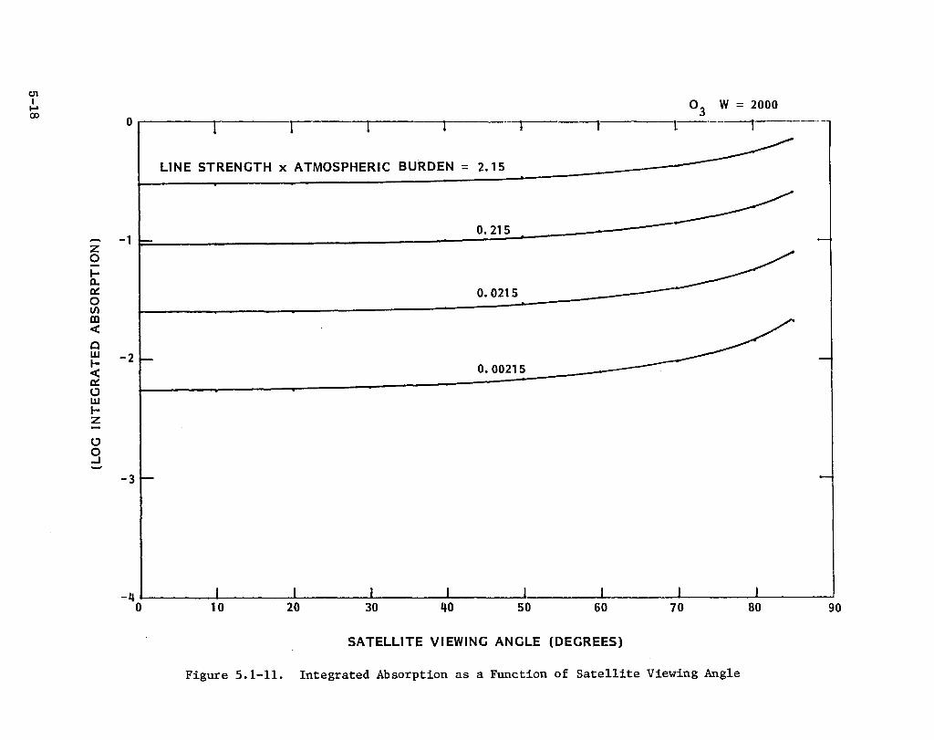
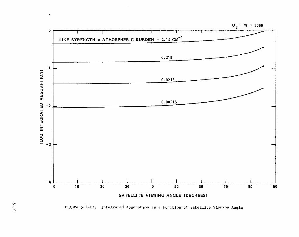
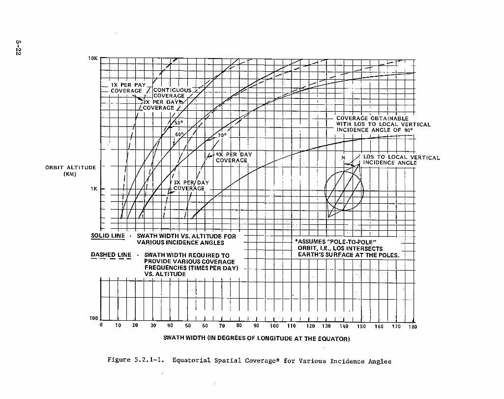
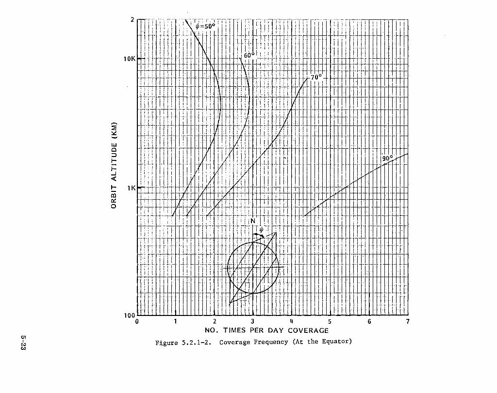
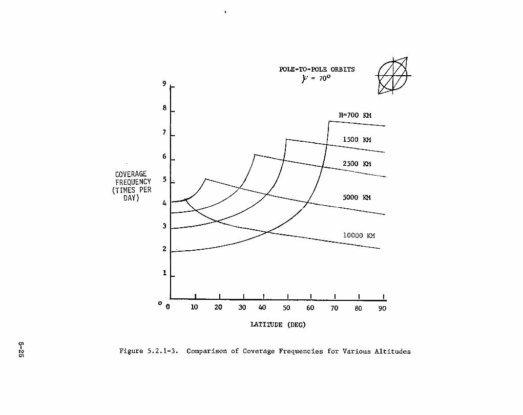
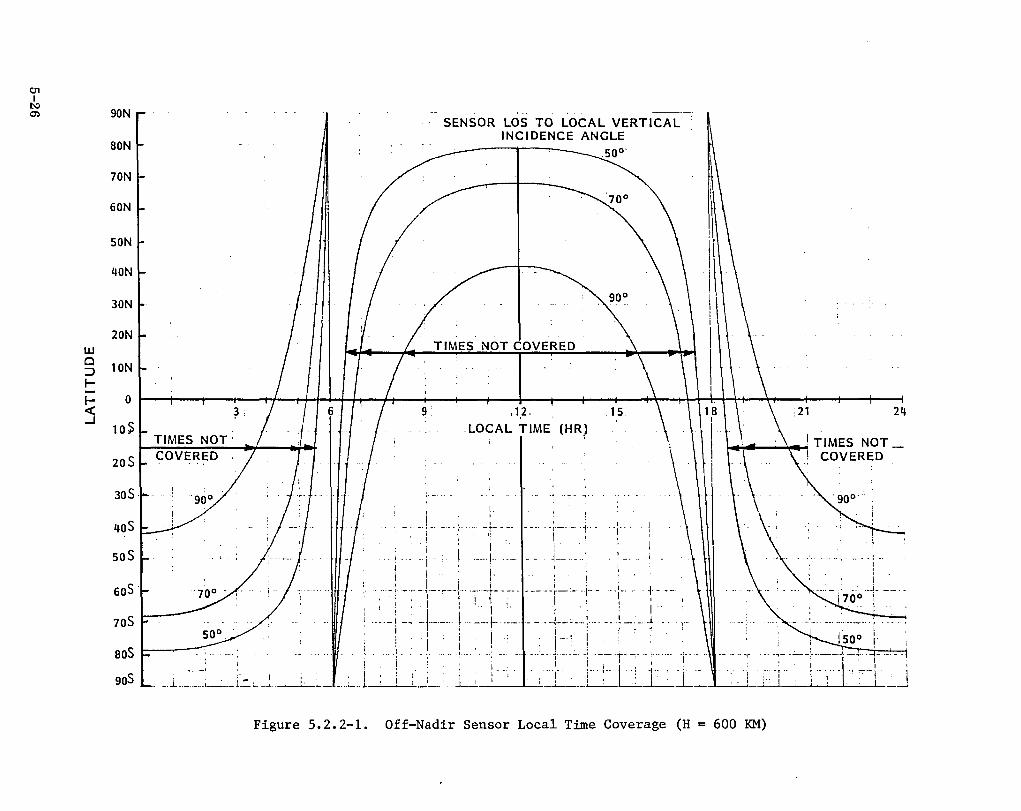

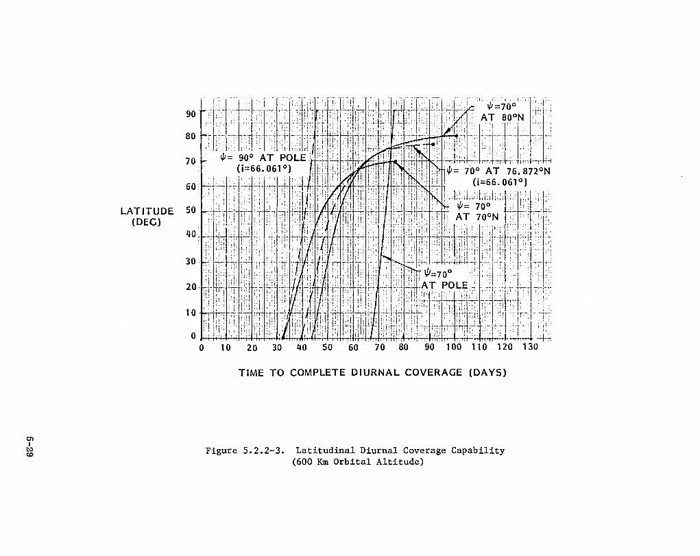
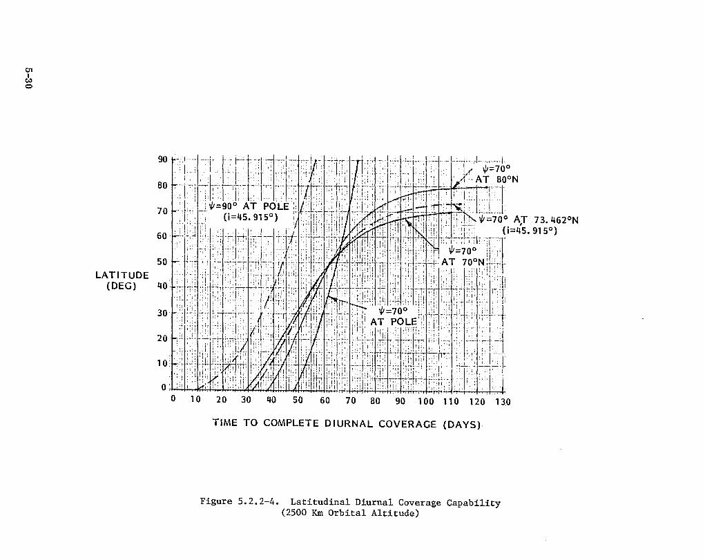

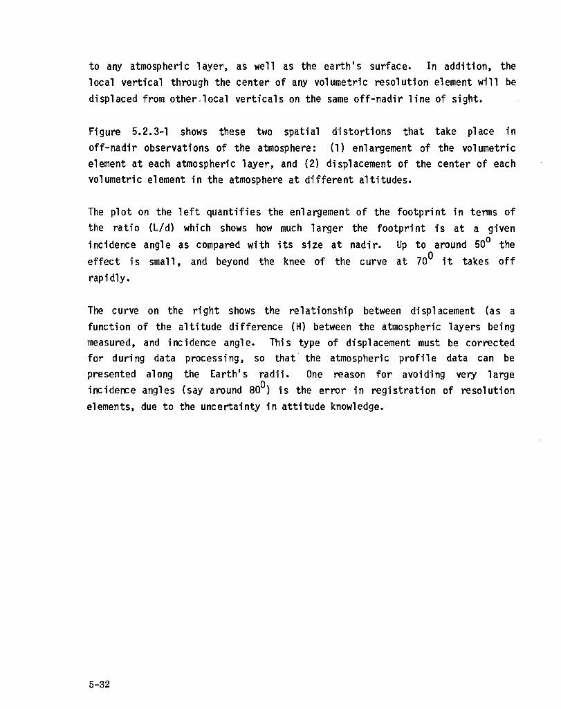
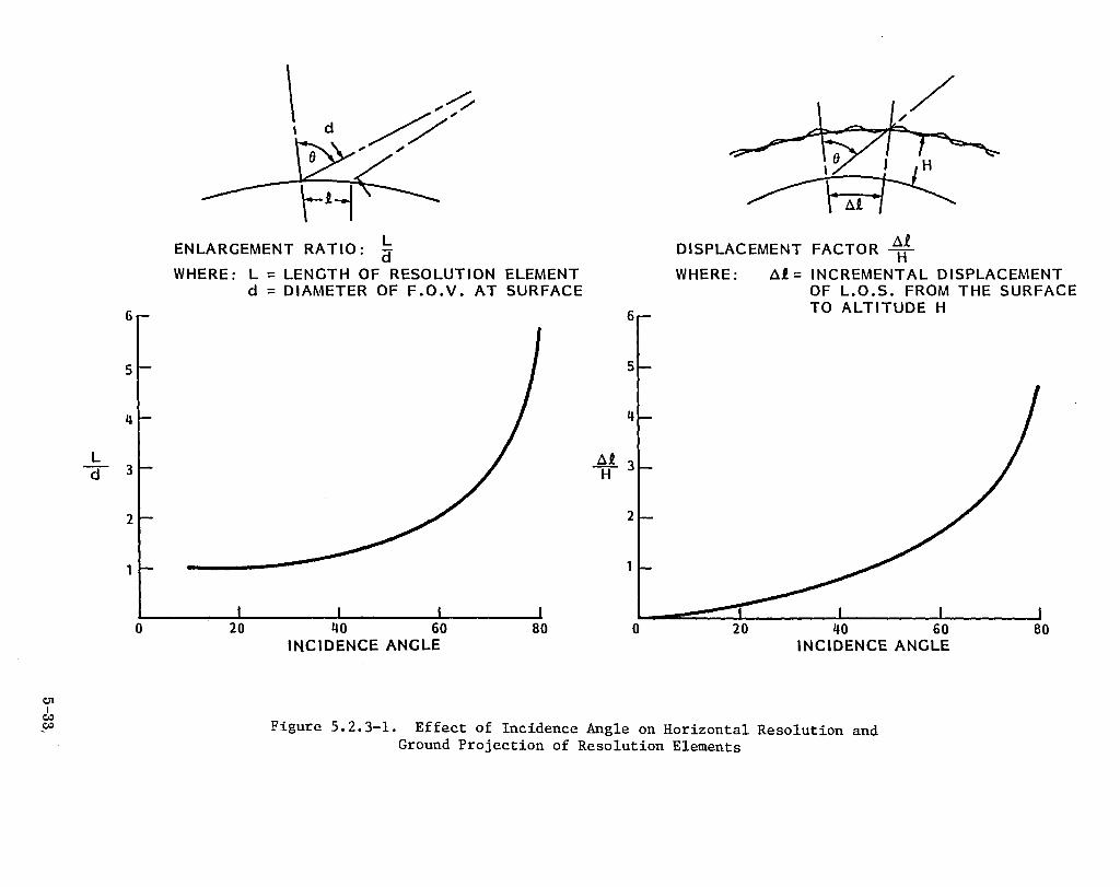
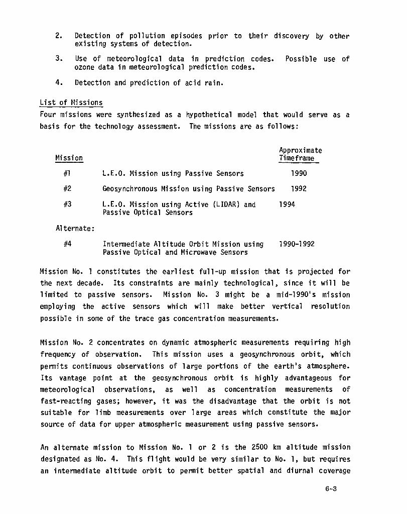
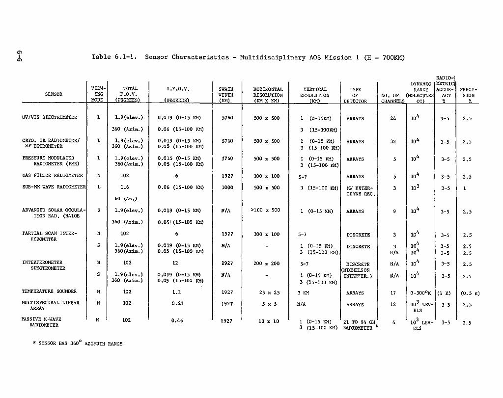
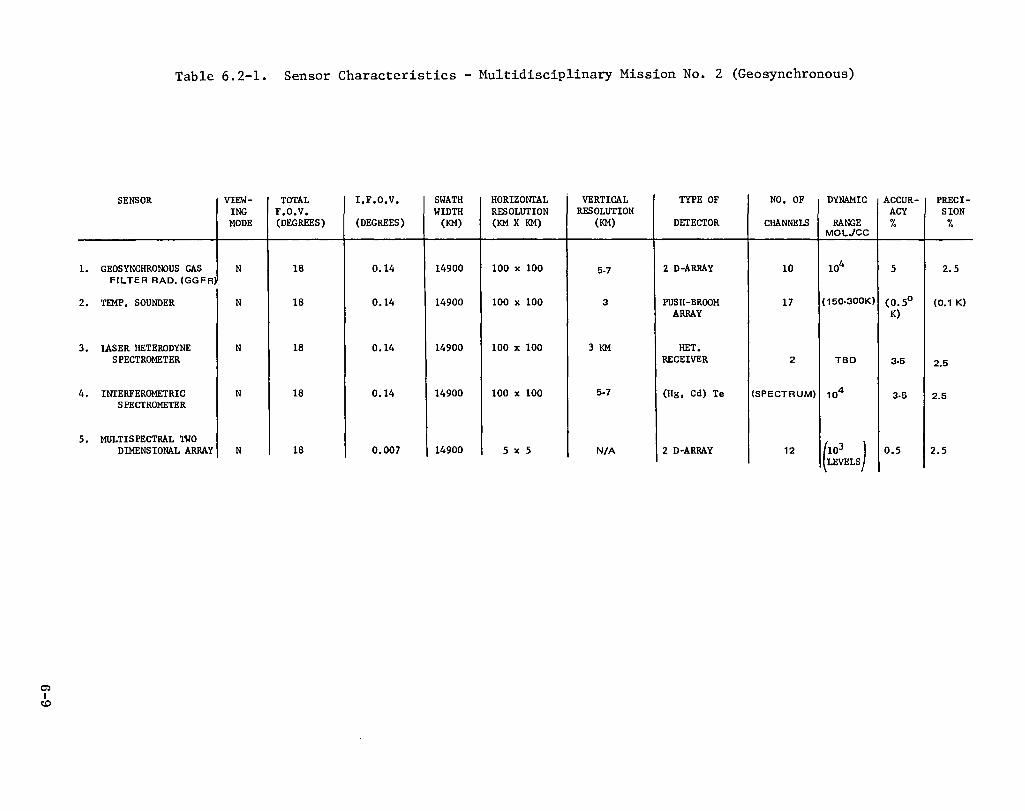
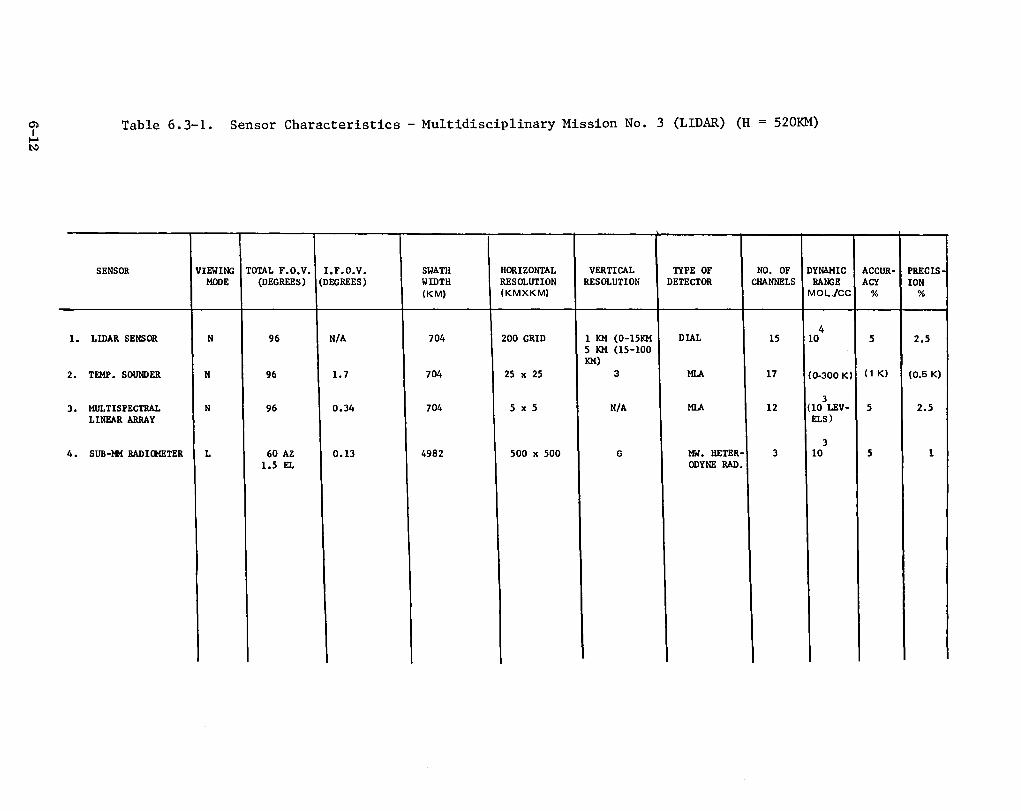
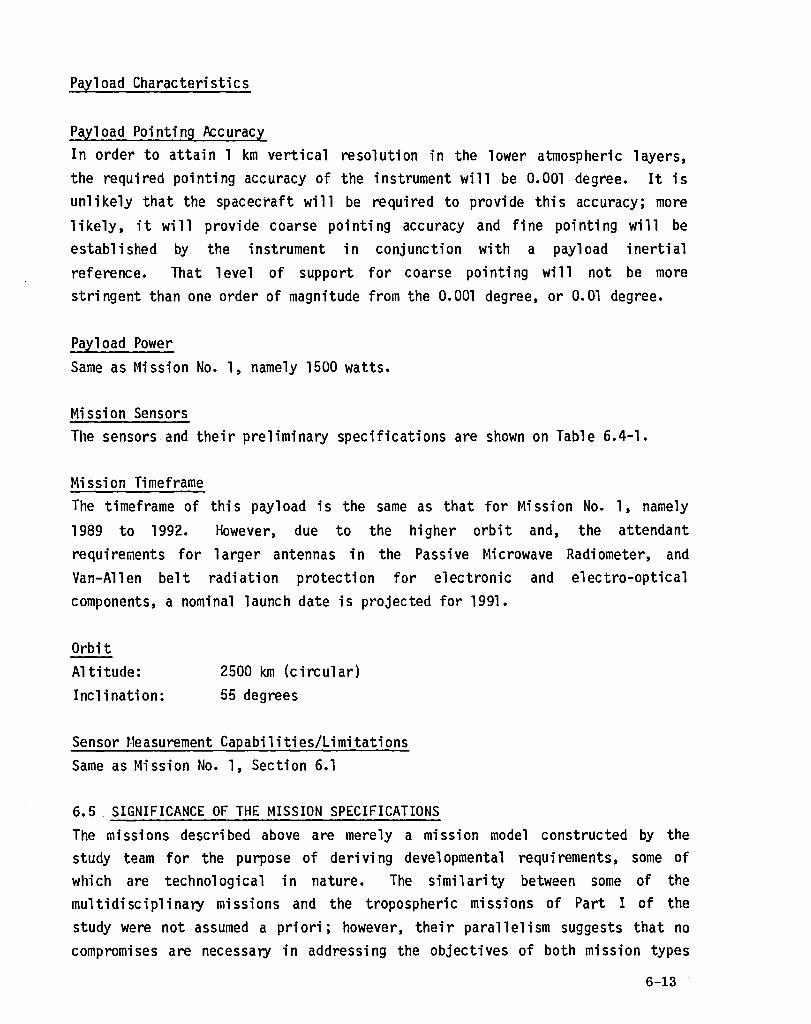
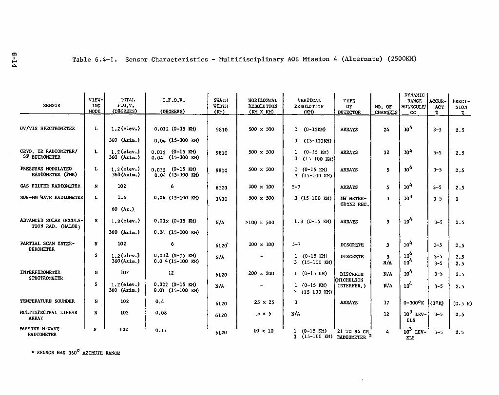

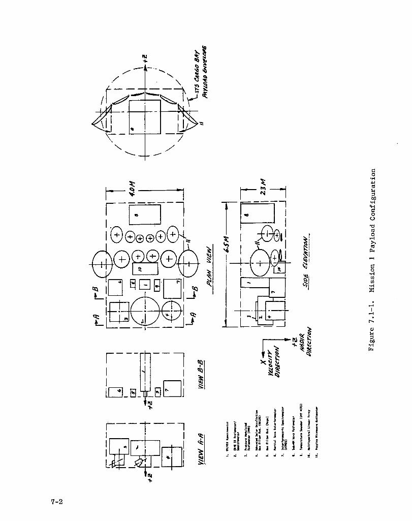
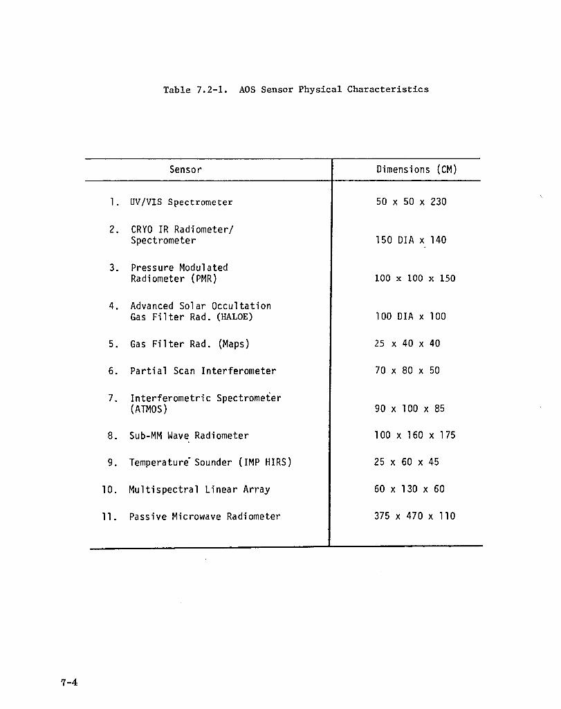
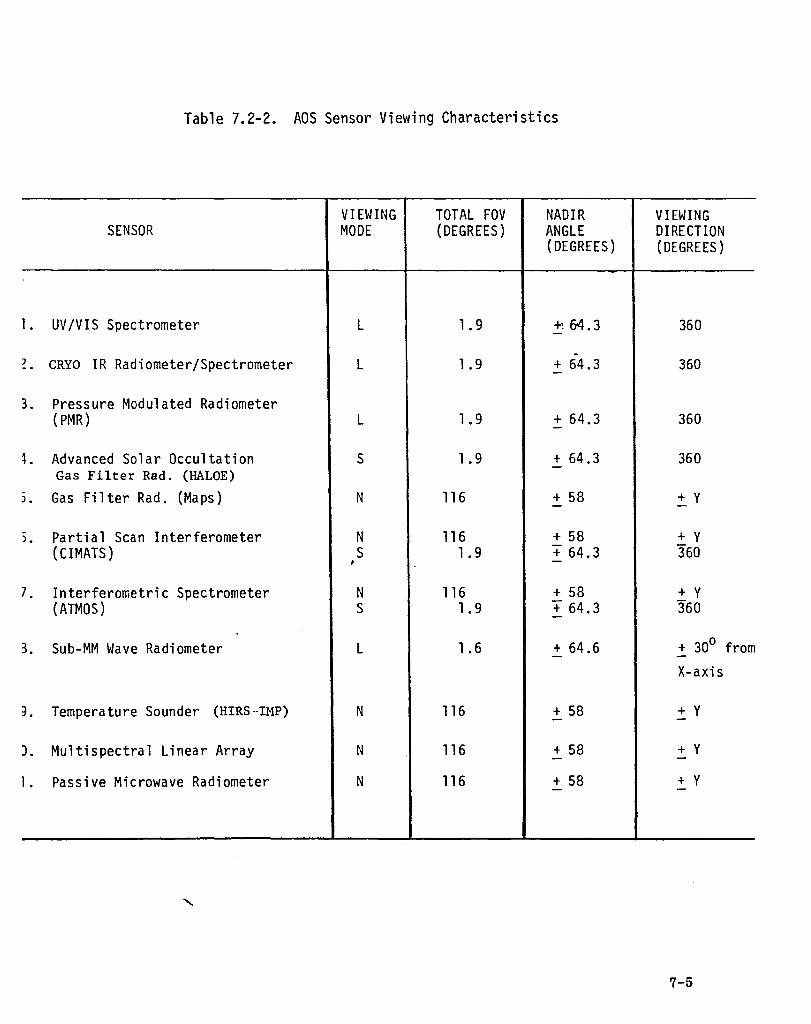
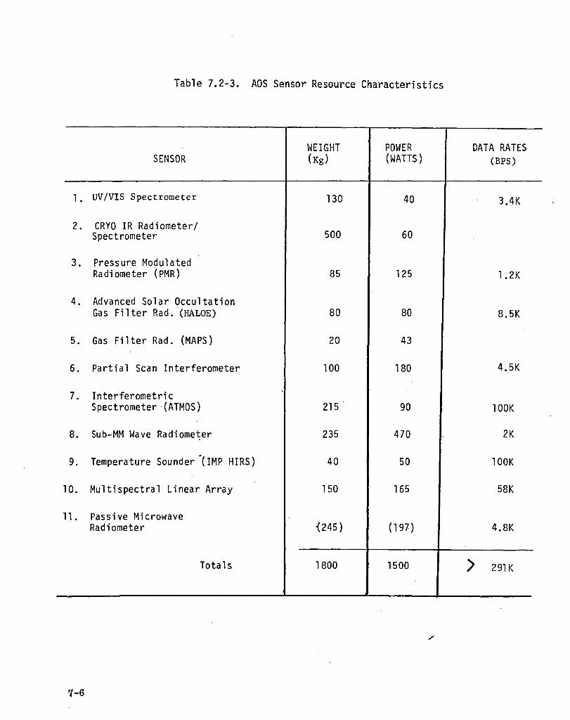
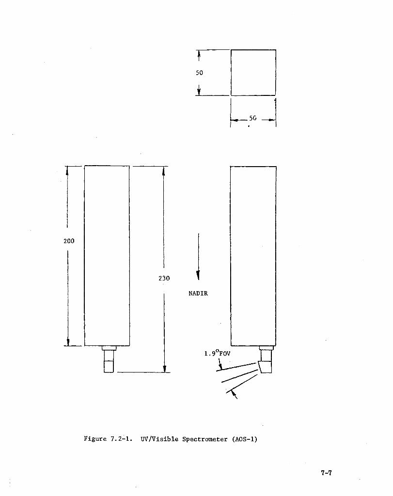
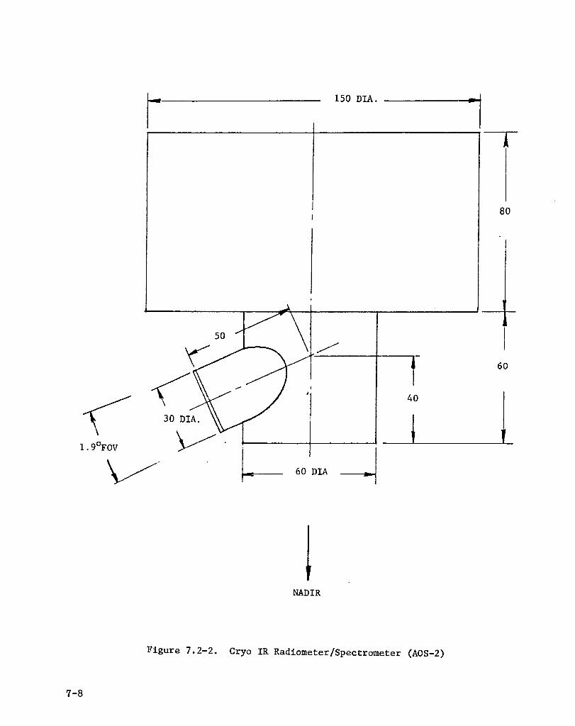
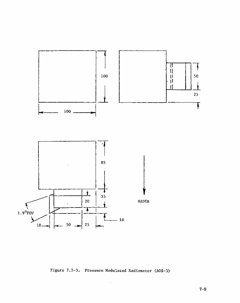
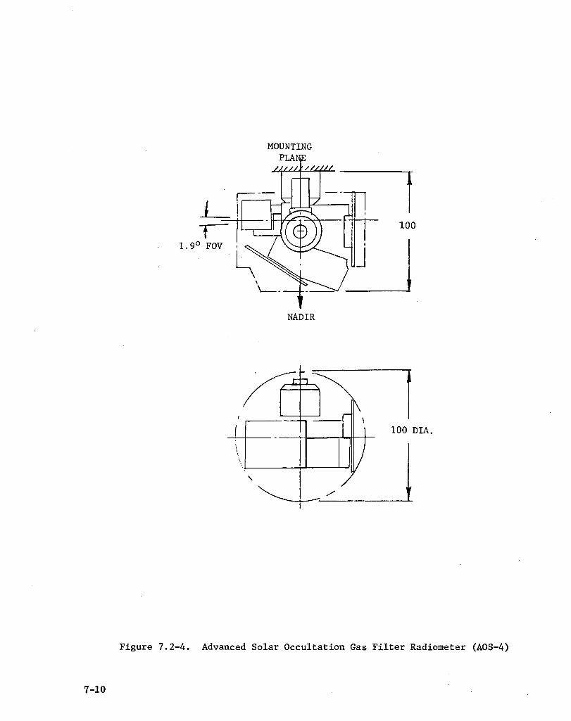
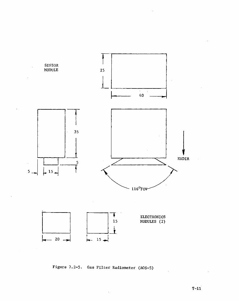
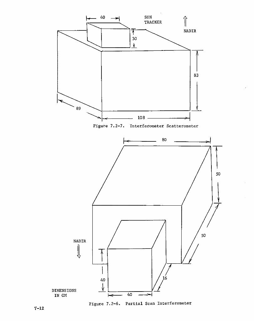

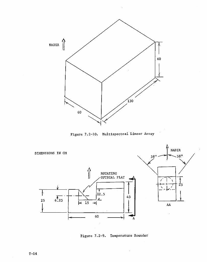
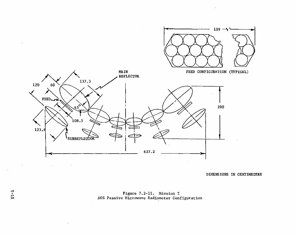
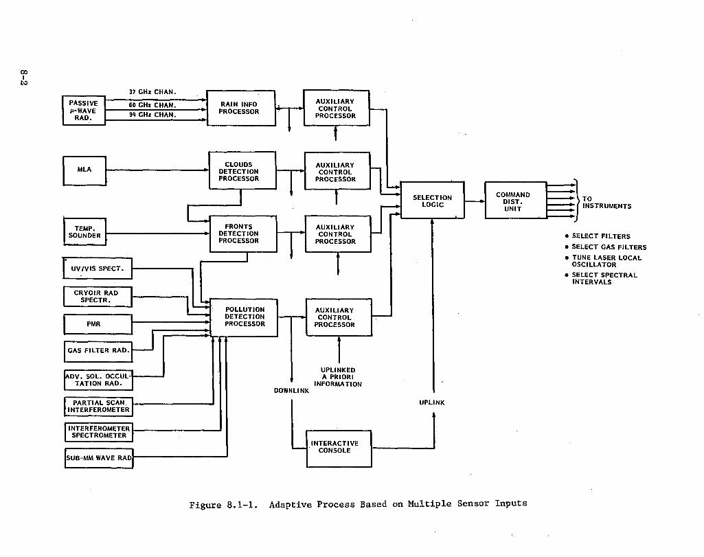
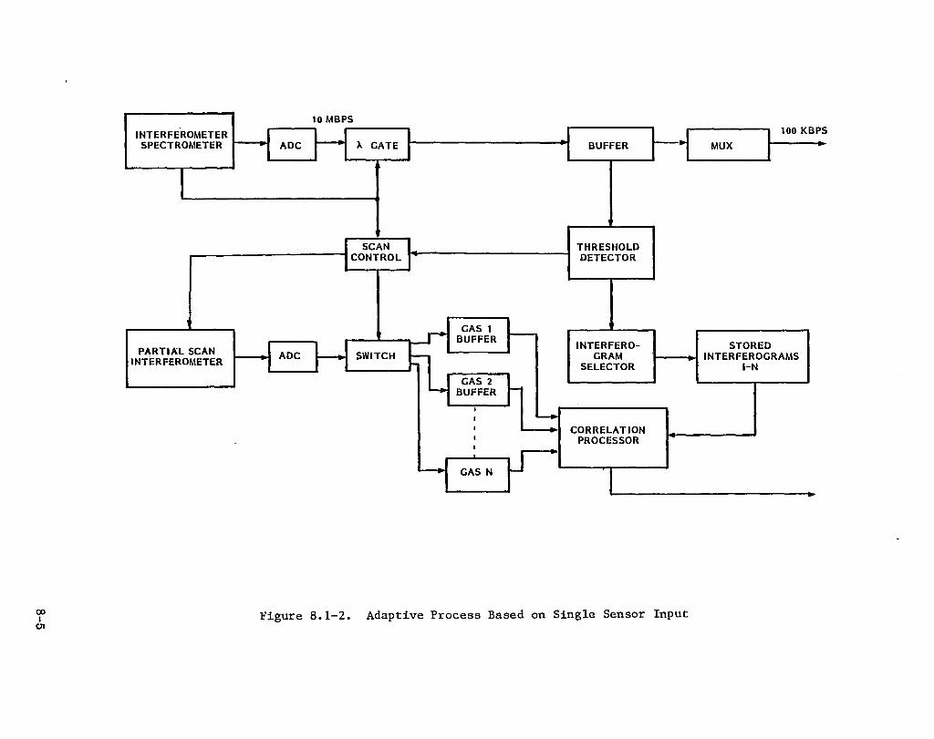
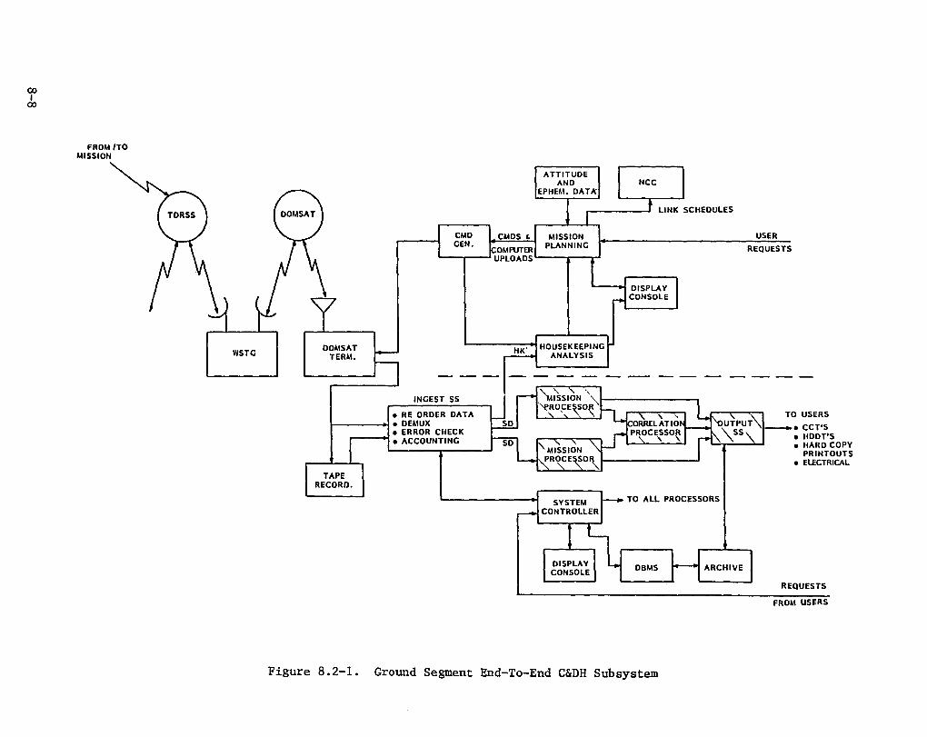
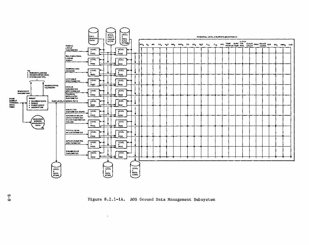
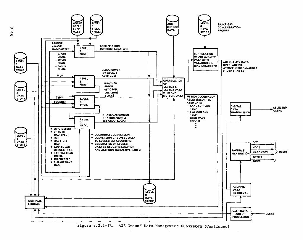
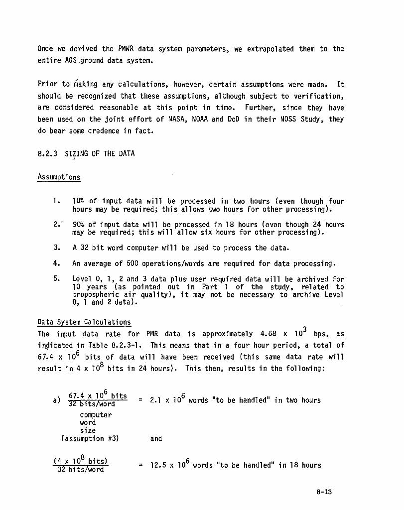
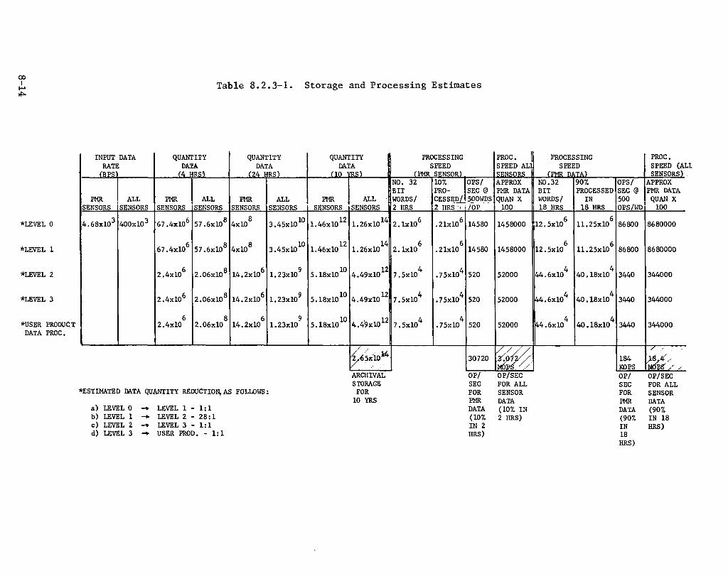
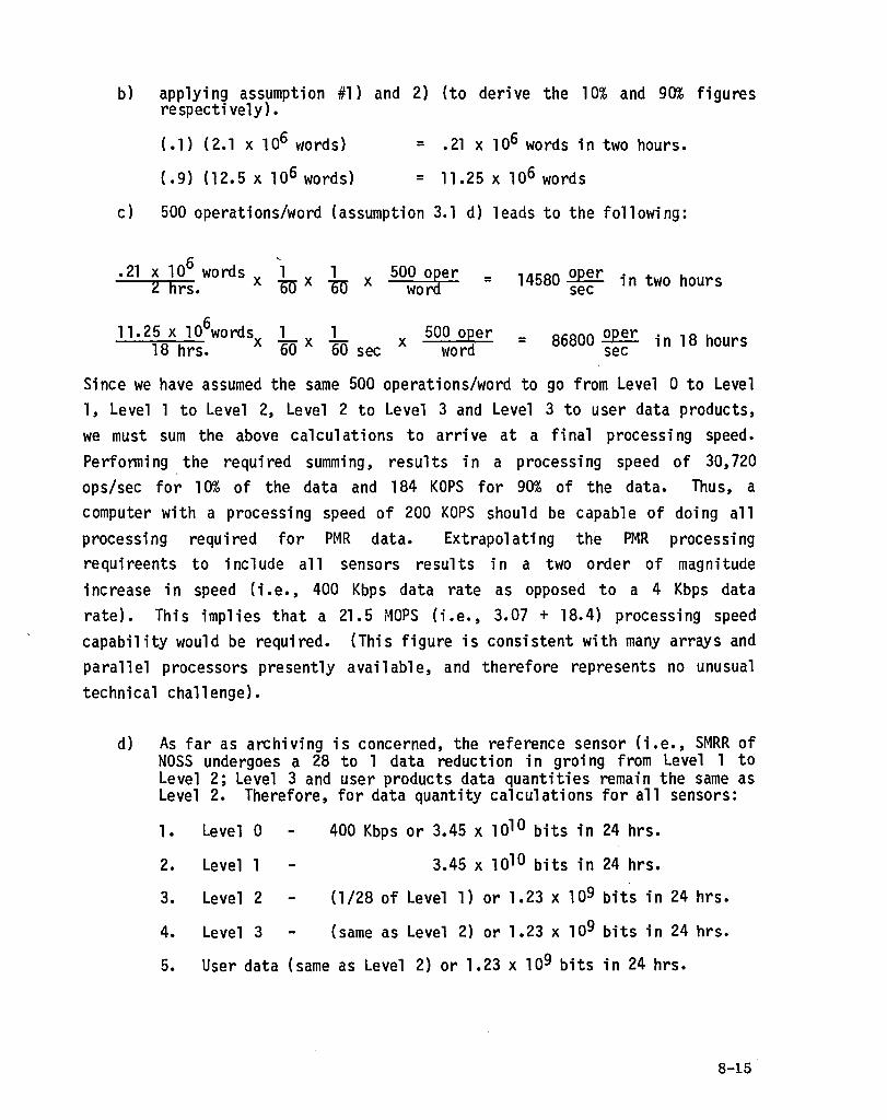

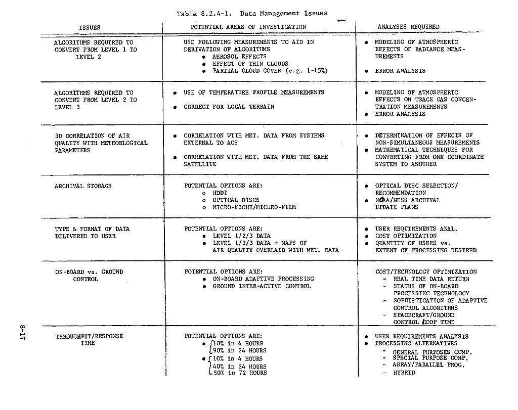
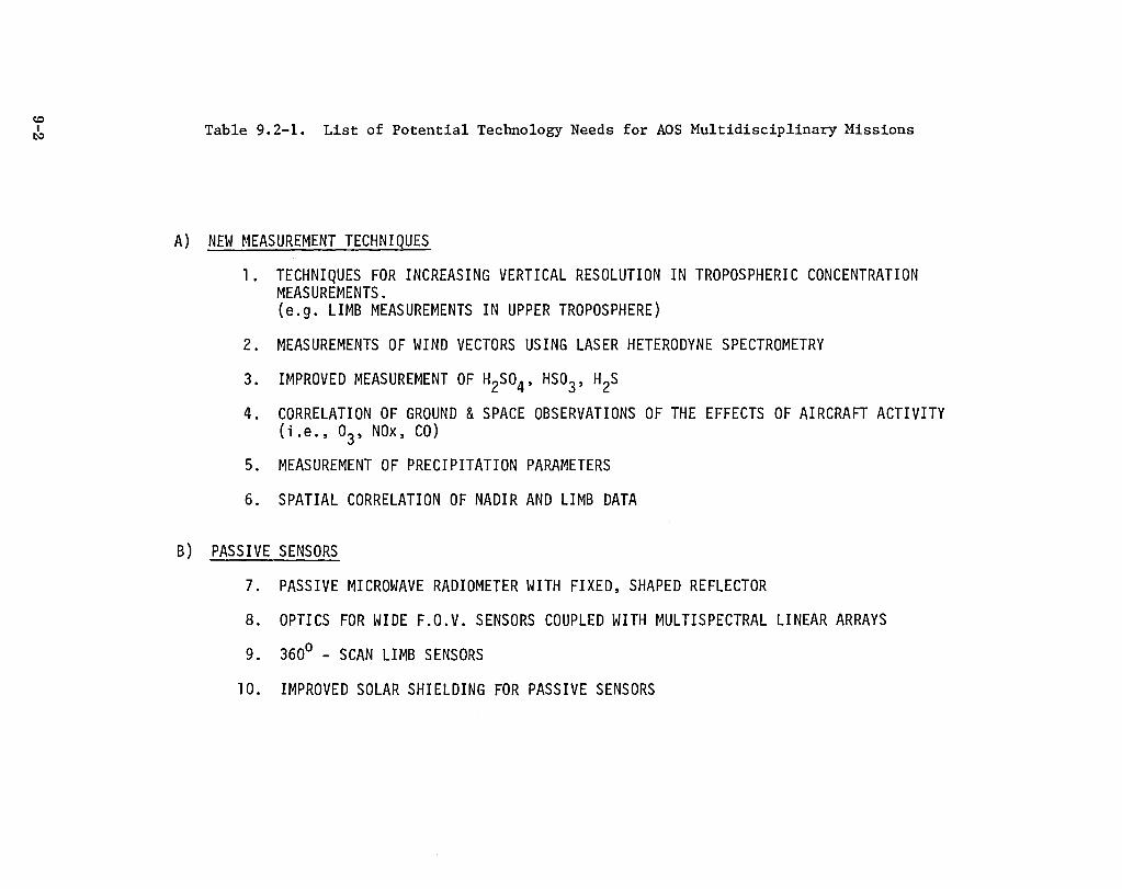
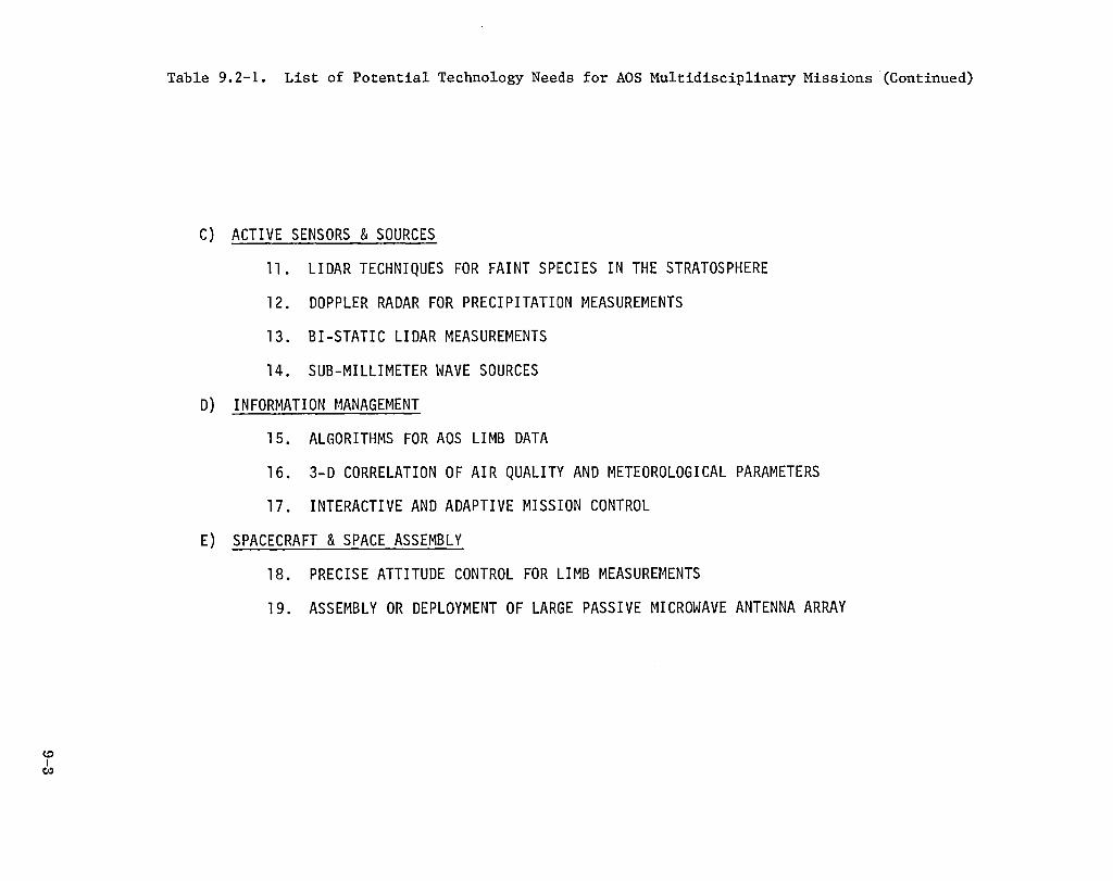
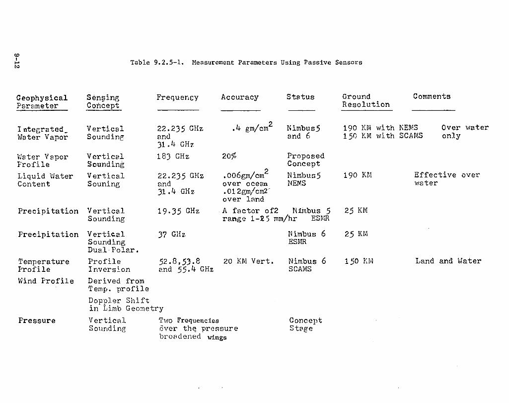
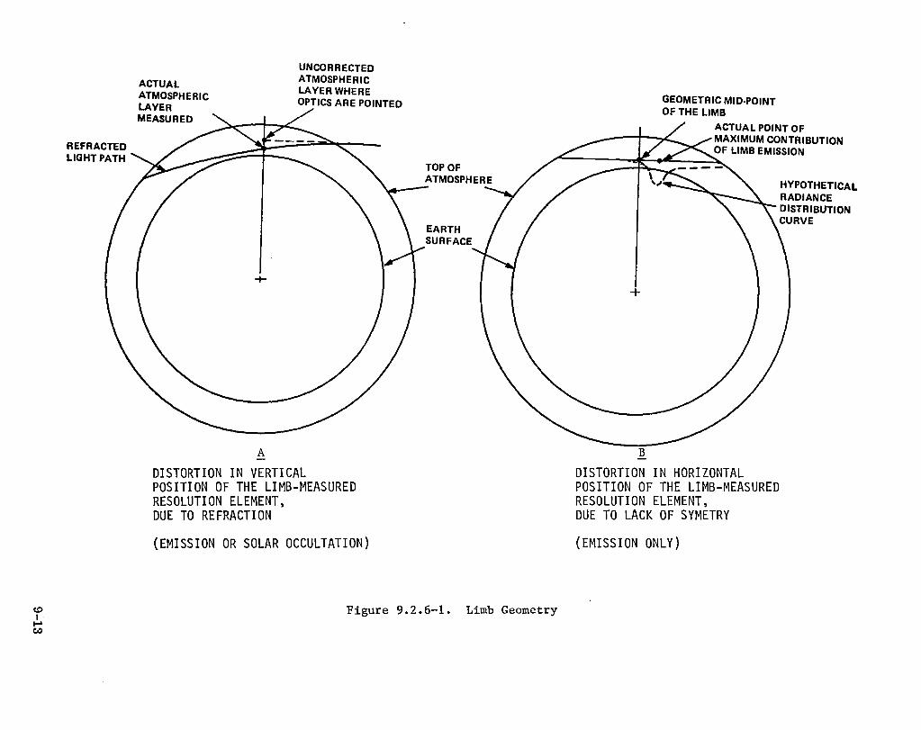
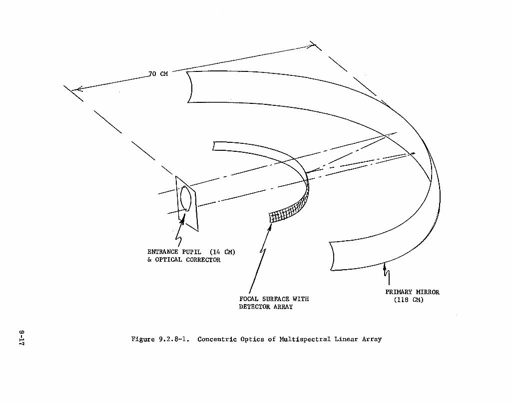
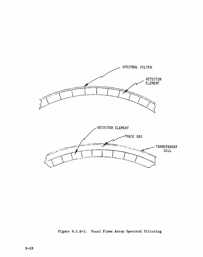
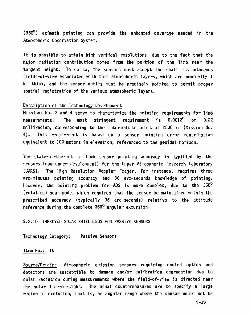
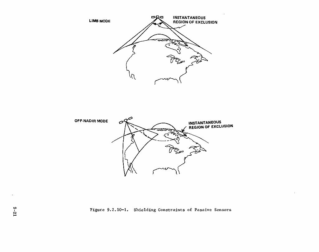
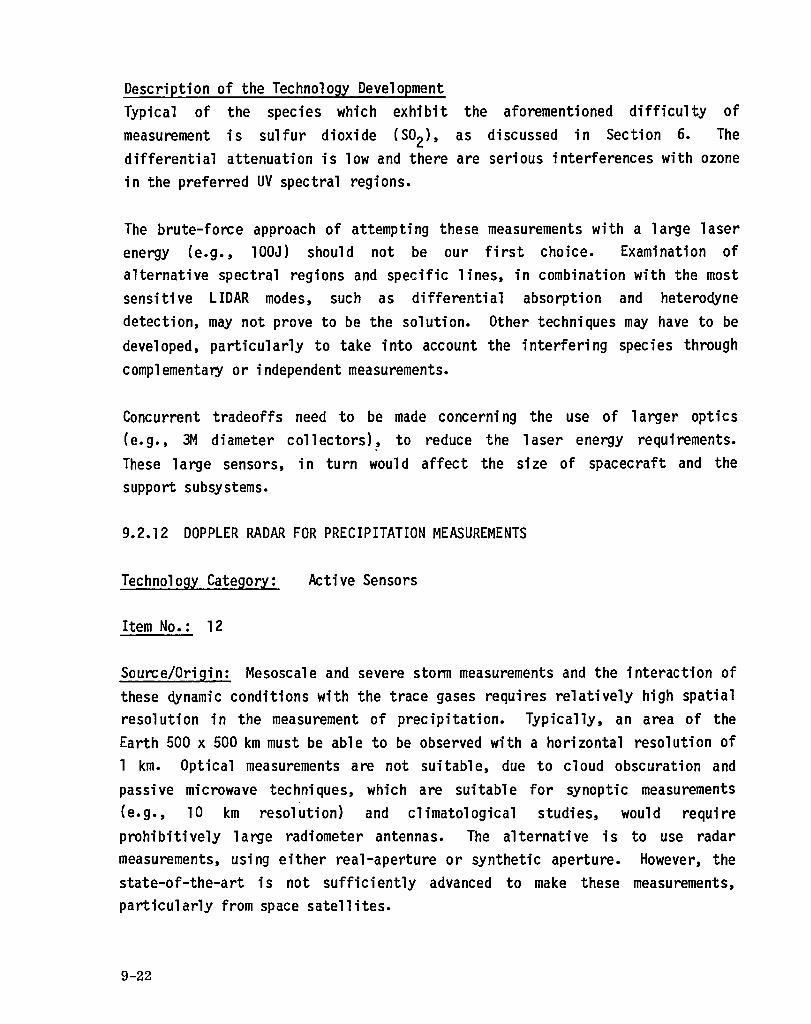
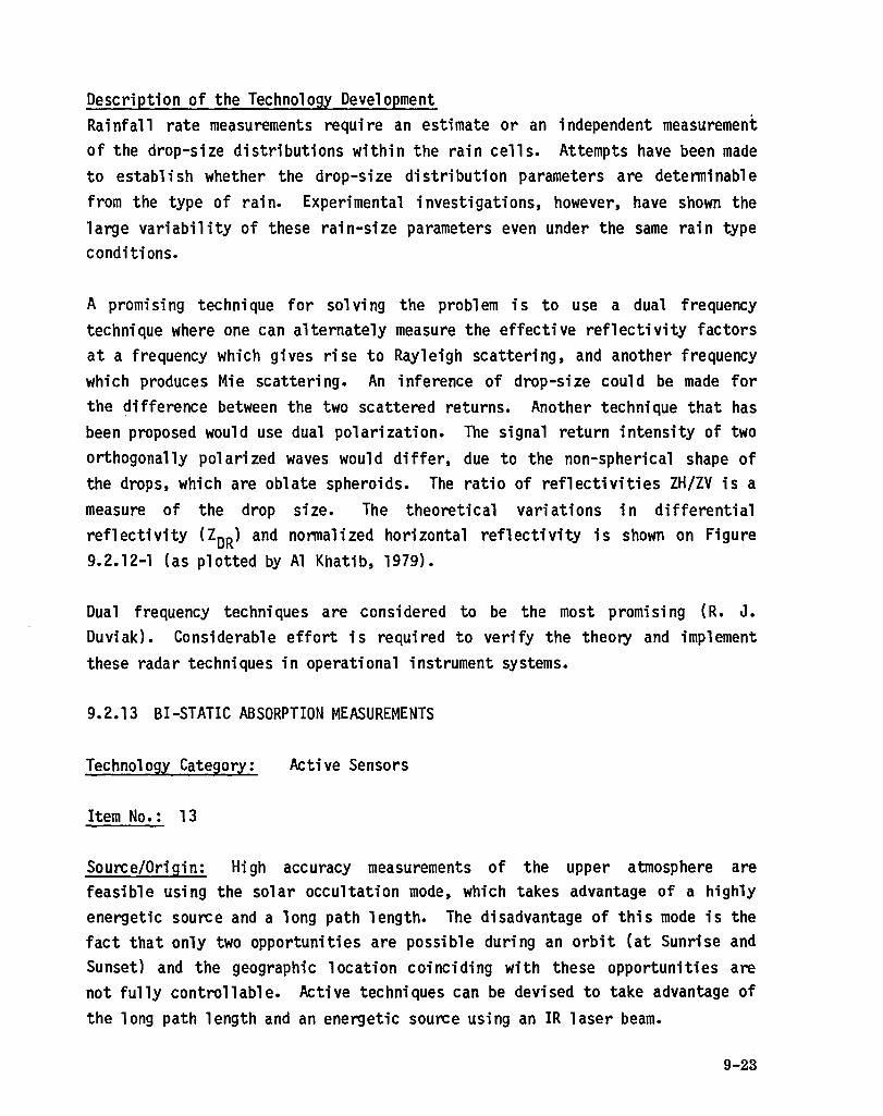
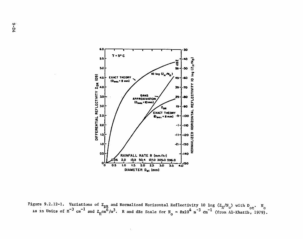

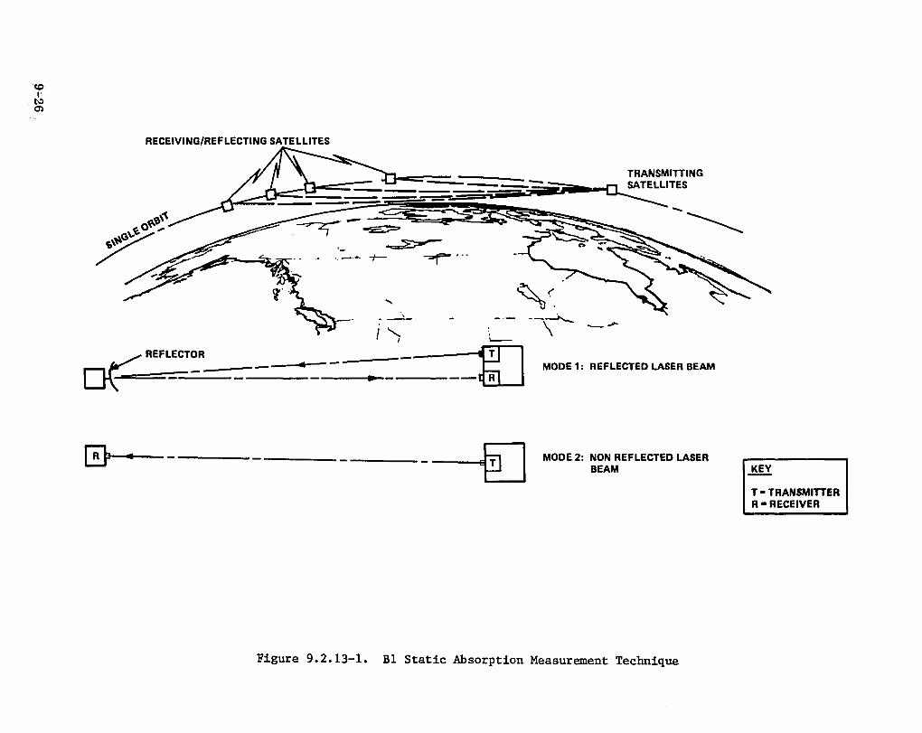
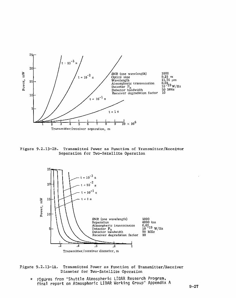
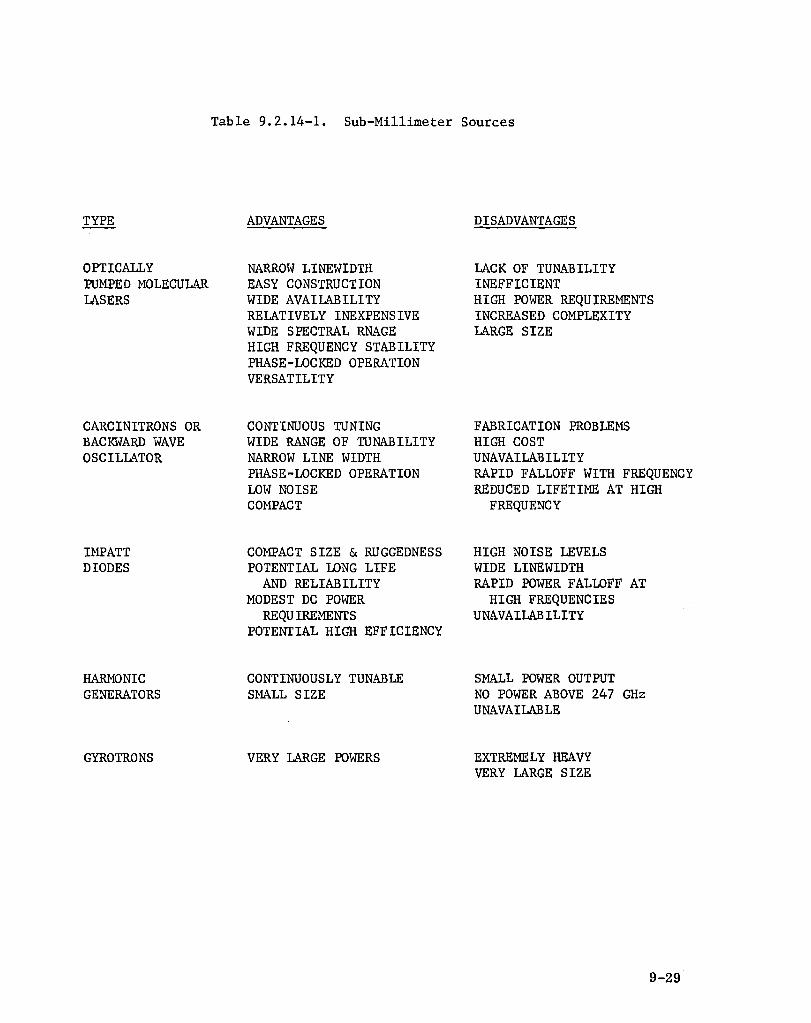
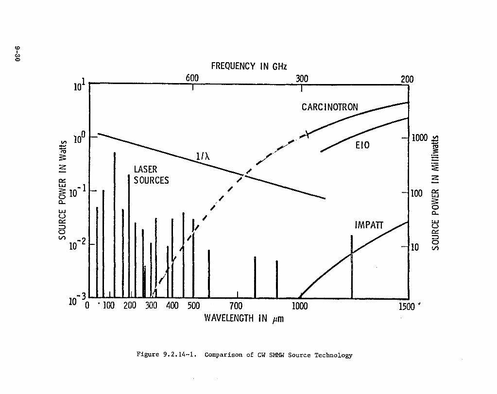
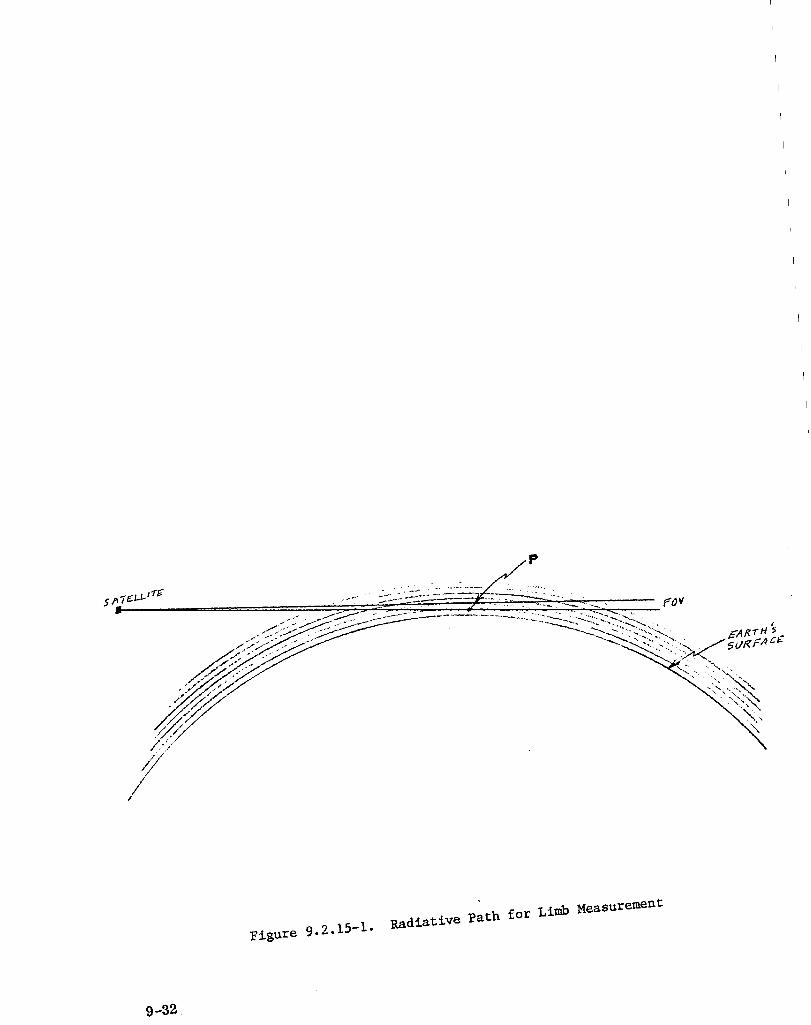
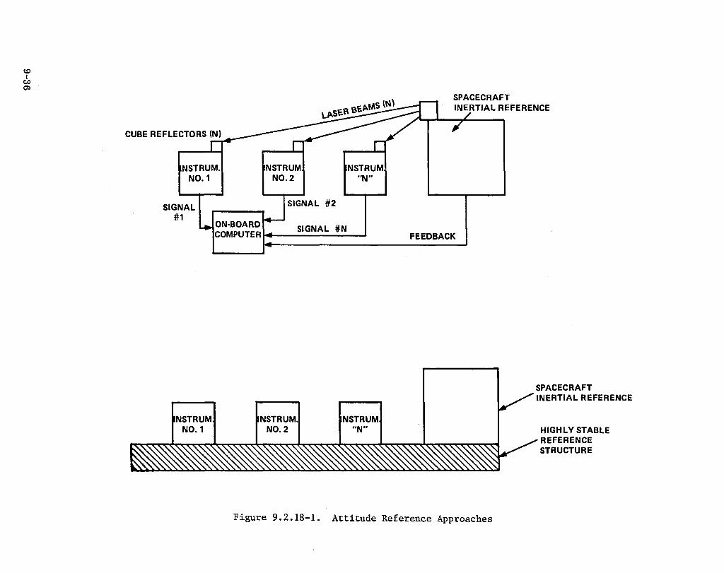
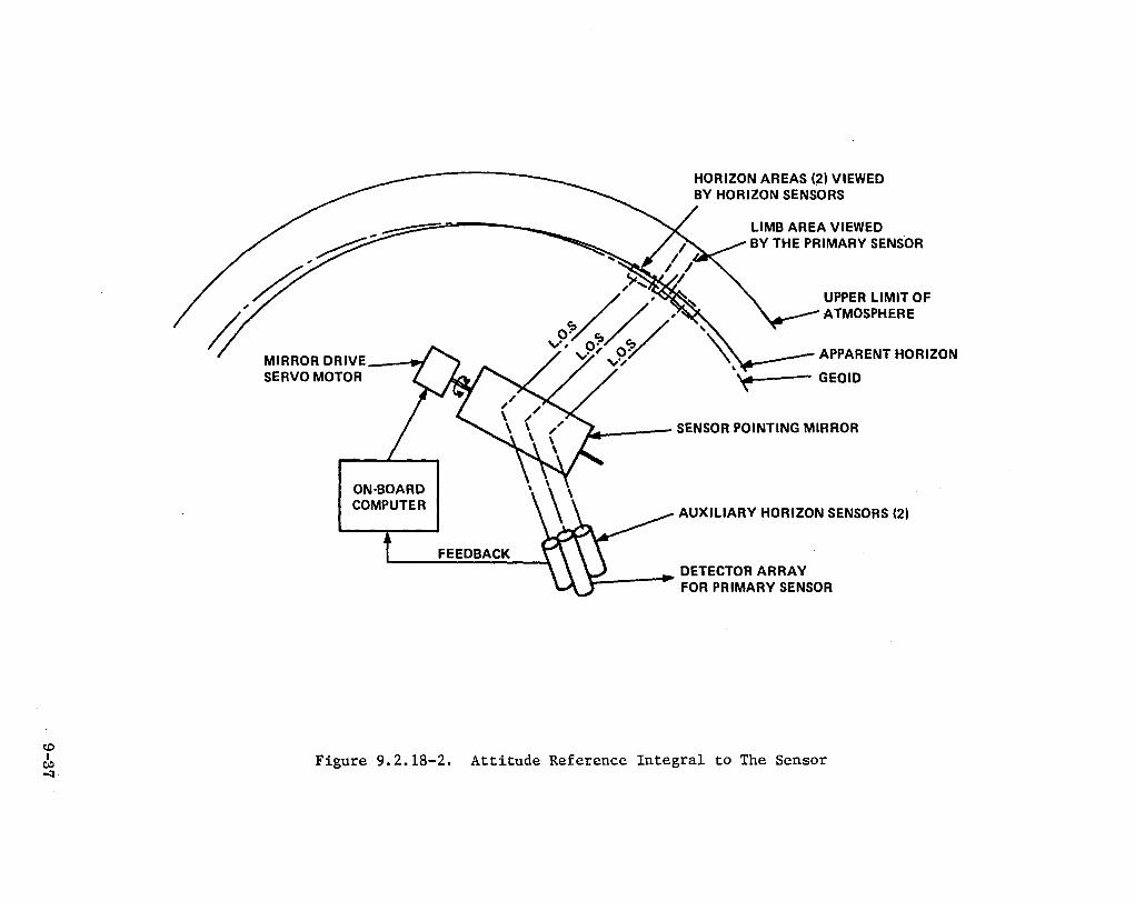
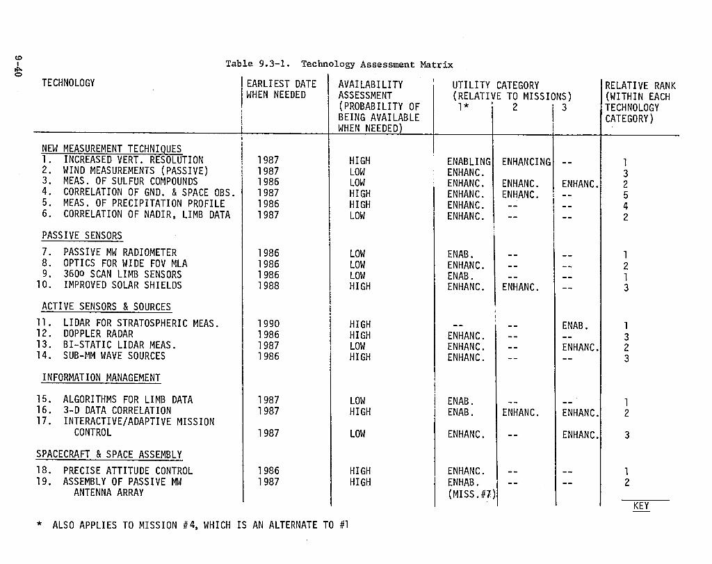
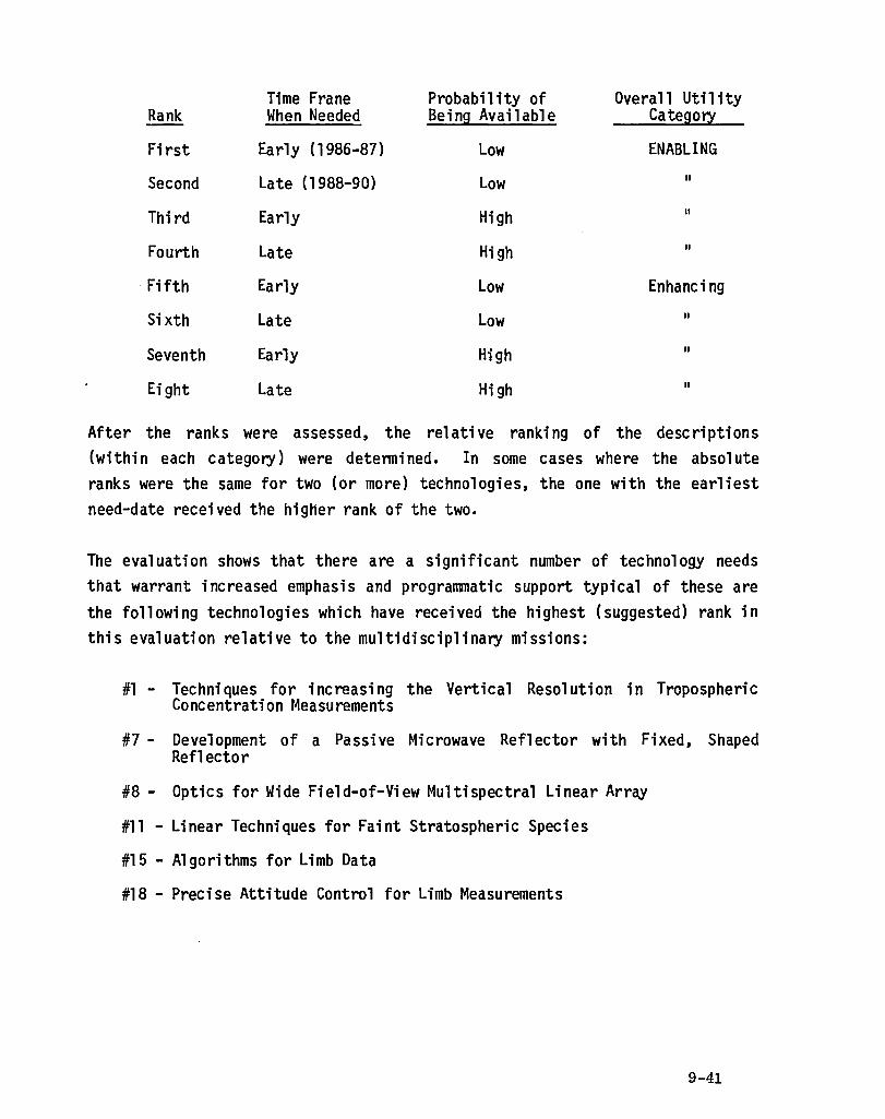
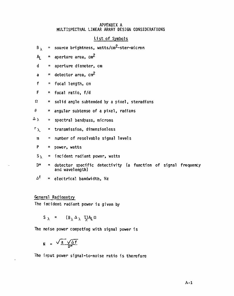
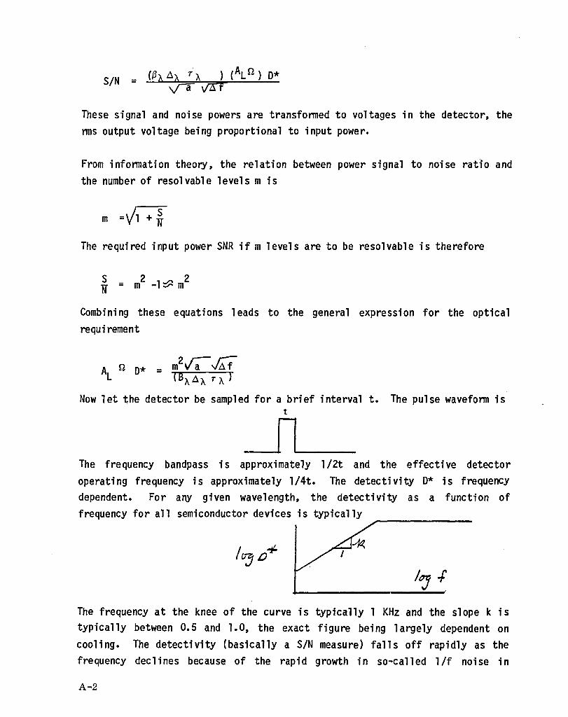
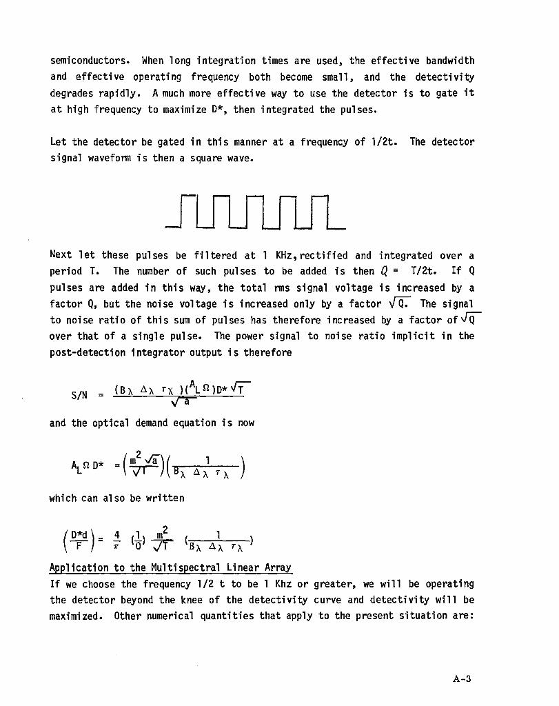
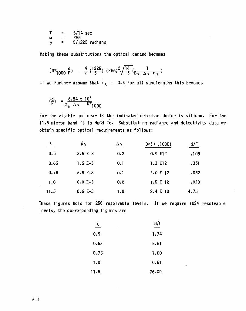
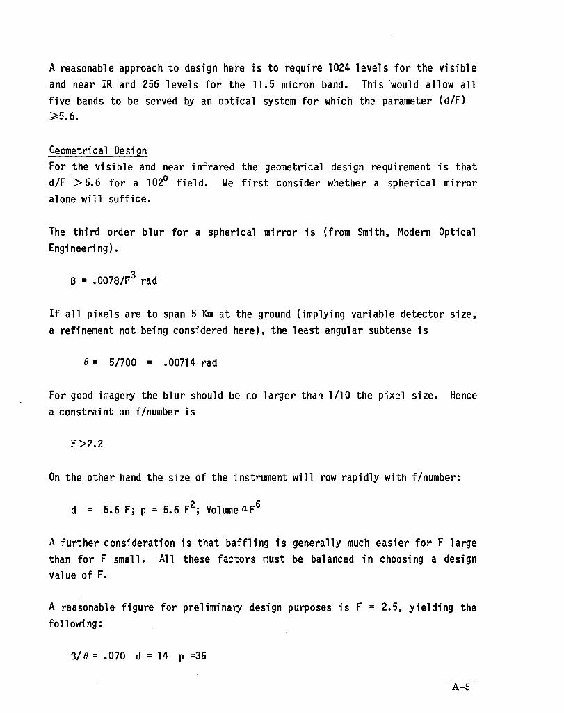


![, NASA Contractor Report ]72 8](https://static.documents.pub/doc/80x56/61f5f30f5bdb351c3b2be492/-nasa-contractor-report-72-8.jpg)

