-- NASA TECHNICAL NOTE NASA TN D-5868 del - -I - m - - - c) - 0 LOAN COPY I+ w Am% nt KIRTLBiND r I+ F r: a m z E PERFORMANCE OF TWIN GYRO ATTITUDE CONTROL SYSTEM INCLUDING PASSIVE COMPENSATION AND NONLINEAR CONTROL LAW by Richard A. Campbell George C. Marshall Space Flight Ceater Marshall Space Flight Ceater, Ala. 35812 NATIONAL AERONAUTICS AND SPACE ADMINISTRATION WASHINGTON, D. C. AUGUST 1970
Transcript
- - N A S A TECHNICAL NOTE NASA TN D-5868 d e l
--I -m---c) -0
LOAN COPY I+ w
Am% nt KIRTLBiND r
I+ Fr: a m zE
PERFORMANCE OF TWIN GYRO ATTITUDE CONTROL SYSTEM INCLUDING PASSIVE COMPENSATION AND NONLINEAR CONTROL LAW
by Richard A. Campbell
George C. Marshall Space Flight Ceater Marshall Space Flight Ceater, Ala. 35812
N A T I O N A L AERONAUTICS A N D SPACE A D M I N I S T R A T I O N W A S H I N G T O N , D. C. A U G U S T 1970
TECH LIBRARY KAFB, NM
~ ._ 1. REPORT NO. 2. GOVERNMENT ACCESSION NO. 3. R E C I P I E N T ' S CATALOG NO.
NASA mJ D~5868- - 4. T I T L E AND S U B T I T L E 5. REPORT DATE
Performance of Twin Gyro Attitude Control System Including A u g u s t 1-970 Passive Compensation and Nonlinear Control Law 6. PERFORMING ORGANIZATION CODE
L 17. AUTHOR(S) 8. PE?FORMING ORGANIZATION REPOR r
George C. Marshall Space might Center I 1 1 .
M209I Marshall Space Flight Center, Alabama 358 12 CONTRACT OR GRANT NO.
13. TYPE OF REPOR-; e PERIOD COVERE SPONSORING AGENCY N A M E AN0 ADDRESS
Technical Note
15. SUPPLEMENTARY NOTES -
Prepared by Astrionics Laboratory, Science and Engineering Directorate
L . 16, ABSTRACT
The first objective of this paper is to determine the effects on the performance of a twin control moment gyro (CMG) attitude control system, when the CMG is attached to the vehicle
The results of the investigation concerning the insertion of the passive compensation network indicate that its principal advantage is to decrease the magnitude of the gyro's developed control torques, thus increasing the bearings lives of the gimbal shafts. The nonlinear control lay accomplished all its objectives. It appears most applicable for space vehicle missions requiring many fast, accurate, large angle maneuvers.
- ~~
17.' KEY WORDS
space vehicles attitude control twin control moment gyro large angle maneuvers fast acquisition time fine pointing accuracy
G electrical parameter of gimbal shaft torque volts/rad motor ohm
Ci viscous damping coefficient of the passive N-m
H angular momentum of gyro rotor N-m-s
29 'J * 2 unit vectors
I.. g the composite mass moment of inertia of the ith 1J
platform's gimbal shaft about its jth axis I
I..P mass moment of inertia of ith
platform about u thits j axis
V principal mass moment of inertia of the vehicle Ii
about its i th
axis (kg-m2)
--K static loop sensitivity
Kfb vehicle attitude feedback gain ( rad/rad)
Ki spring rate of the passive compensation N-m
network for the ith platform rad
thKmi gimbal shaft torque motor gain for the i N-m
platform rad
R armature resistance of gimbal shaft torque (ohms)motor
viii
L IST OF SYMBOLS (Continued)
Symbol Definition Unit
r Y PY q components of the vehicle angular velocity ( rad/sec)
ri * p: q.* components of the ith platform's angular
( rad/sec)1 velocity
T torque acting on the gimbal shaft (N-m)
Text. 1
external disturbance torque acting about
the vehicle's ith axis
(N-m)
Tmi torque generated by the ith platform's gimbal
shaft torque motor (N-m)
Tt torque developed by a jet thruster (N-m)
V 0
voltage applied to the gimbal shaft during nonlinear operation
(volts)
x ,y , z vehiclefixed coordinate system
P , 01, relative angular displacement between the gyro-platform-fixed coordinate system and (rad) the vehicle-fixed coordinate system
6, Pl Y gimbal angles of the X-, Y-, and Z-axis CMG's respectively (rad)
0 Y @ Y + vehicle's Euler angles (rad)
r torque acting on the gyro rotor (N-m)
A0 0 linearity limits of the nonlinear control function (rad)
8 vehicle attitude command ( rad)C
8V
vehicle's attitude (rad)
ix
I ll1l1111l1lll I I I
LIST OF SYMBOLS (Concluded)
Symbol Definition Unit
t damping ratio
T torque acting on the vehicle
X deflection of light source image
-X measured light source deflection by the
radiation tracking transducer
w angular velocity of the vehicle with respect to an inertial reference
w* angular velocity of ith platform with respect
i to an inertial reference
w natural frequencyn
ACKNOWLEDGMENTS Grateful acknowledgment is given Dr. Walter Haeussermann for serving as
technical advisor and I also wish to thank Mr. J. C. Farr ish, J r . , fo r acting as lead design engineer for all the experimental hardware; Mr. W. W. Woods and M r . D. C . Williams, for providing the detailed designs of the experimental hardware; Mr . H. C . Haven and M r . A. D. Reasor, for the fine workmanship they performed in machining and assembling the experimental hardware; and M r . R. L. Keefer, for his efforts in programing the analog computer.
X
i 1
Q F
.._. .. . ... i
PERFORMANCE OF TWIN GYRO ATTITUDE CONTROL SYSTEM INCLUDING PASSIVE COMPENSATION AND
NONL I NEAR CONTROL LAW
INTRODUCTION
Newton's second law, the Principle of Conservation of Angular Momentum, forms the foundation upon which all attitude control systems are based. These systems a r e categorized as being either active, passive, o r semipassive.
An active control system is defined as one that requires some form of onboard power. These a r e generally closed-loop systems requiring some form of sensor to provide the feedback signal [ I]; that is, instrument gyro, sun sensor, horizon sensor, o r s tar tracker. These types of systems are employed for missions requiring high pointing accuracy o r for performing complex maneuvers. The torque-producing devices for such systems a r e reaction control jets (RCJ's) , reaction wheels, o r control moment gyros (CMG's) .
Passive control systems a r e defined as those systems that do not require onboard power, but rather they make use of such natural phenomena a s solar radiation, magnetic gradients, and gravity gradient [2-41 . These a r e open-loop systems with very large time constants. Systems of this type have been used on weather satellites where long mission life and high reliability a r e key factors.
In some cases it is possible to replace active components with passive components, thereby forming a hybrid system referred to as "semipassive. " These systems take advantage of the power savings and high reliability of passive components and yet retain the advantages of the active systems.
For vehicles requiring very accurate and continuous control, the CMG is the superior device from the standpoints of power, accuracy, response, and simplicity [51 .
A CMG consists basically of a rotor with a certain constant magnitude of angular momentum and a mechanism used to precess the rotor. The configuration of this precession mechanism determines the cross coupling characteristics of the generated control torques. There a r e three basic configurations of precession mechanisms referred to as one degree of freedom, two degrees of freedom, and the twin gyro ( Fig. i).
The one-degree-of-freedom CMG, Figure ia, consists of a rotor mounted on a gimbaled shaft driven by a torque motor. The developed control torque lies in a plane perpendicular to the gimbal shaft, thus producing two-axis cross coupling. This control torque is transmitted through the gimbal axis bearings to the vehicle. A control system composed of three one-degree-of-freedom CMG's was discussed and analyzed by White and Hansen [ 61. These systems were shown to be severely c ross coupled and required a very complex control computer to decouple the control torques so that three-axis control could be attained. A failure of any one CMG would cause the loss of three-axis control.
The two-degrees-of-freedom CMG consists of a rotor mounted so that it is capable of being precessed about two axes. This is accomplished by the double-gimbal precession mechanism shown in Figure ib. This mechanism requires two torque motors, one for each of the gimbal axes, which must be capable of transmitting the control torques to the vehicle. This type of precession mechanism produces three-axis cross coupling of the control torque. A minimum of two two-degrees-of-freedom CMG's a r e required to obtain three-axis attitude control. This system is also severely cross coupled and requires a very complex control computer for its implementation [ 7 , 8 ] . Unlike the one-degree-offreedom CMG system, this system is 33 percent redundant with respect to its torque motors; that is , should one motor fail, this system would still be able to provide three-axis control.
The third configuration, the twin gyro shown in Figure IC, consists of two one-degree-of-freedom CMG's geared together s o that their angular momentum vectors always remain in a position that is the mirror image of the other. This configuration, like the one degree of freedom, requires only one torque motor and permits the control torques to be transmitted through the gimbal shaft bearings to the vehicle, The major advantage of this configuration over the previous two is that it eliminates the first-order cross coupling terms, thereby forming a single-axis control device. A minimum of three twin CMG's a r e required for three-axis attitude control [91 . This control system possesses only second-order cross coupling effects and therefore requires the simplest control computer. While it is true that the weight and power requirements a re greater for this system than for either of the two systems mentioned previously, this system does possess 100 percent redundancy with respect to its rotors; that is , three-axis control can be maintained with one rotor failure for each twin gyro. However, with the loss of a rotor the twin gyro is transformed into a single-degree-of-freedom gyro; thus, an alternate control law must be implemented by the control computer to facilitate the two-axis cross coupling present. It is the opinion of H.B . Kennedy [ I O ] that the reliability of the twin CMG is greater than that of the two-degree-of-freedom CMG because of the reduced number of gimbals and gyro bearings.
2
a. One Degree of Freedom
b. Two Degrees of Freedom
W W6
c. TwinGyro
Figure I.Control moment gyros. 3
11111lIIllIllIl l1llll11l11l11l I Ill I1
Throughout this paper the complete assemblage of the twin CMG will be referred to a s being a gyro platform. When these platforms a re fastened rigidly to the vehicle structure, they a r e referred to as being rigid. When the platforms a re fastened by means of a spring-damper mechanism, they a re referred to as being compensated.
DERIVATION OF CONTROL EQUATIONS FOR A VEHICLE W ITH R IG I D PLATFORMS
Consider a three-axis attitude control system which is composed of three twin CMG platforms, as shown in Figure 2. The assumptions made for the derivation of the equations of motion for this system a r e as follows:
I.The gyro platforms are rigidly fastened to the vehicle structure; that is, the vehicle-fixed coordinate system corresponds to the gyro-platformfixed coordinate system.
2. The mass moments of inertia of each rotor and each of their gimbal structures a r e equal.
3. The magnitudes of the rotor's angular momentum vectors a re equal and constant.
4. No mass unbalance exists about the gimbal axis; that is, the center of mass of the gyros lies on the gimbal axis.
The three CMG platforms shown in Figure 2 a re designated as X, Y, and Z , corresponding to the vehicle's X-, Y-, and Z-axes, respectively. These platforms are aligned so that the developed control torques act along the vehicle's principal axis.
A vector schematic of the X-axis platform is shown in Figure 3. The angular momentum vector of each gyro is designated H and H
x2 . The
X i first subscript associates the angular momentum vector with a particular platform; the second subscript indicates the gimbal axis, axis Ibeing the torquer-driven shaft. The angular momentum vectors, written in terms of the vehicle-fixed coordinates, a r e
4 f
IZVEHICLE
Z PLATFORM
EDDY CURRENT DAMPER
Y PLATFORM
X PLATFORM
YVEH ICLE
Figure 2. Three-axis twin control moment gyro control system.
5
1111l11ll1 I I
z INERTIAL REFERENCE
ZVEHICLE
x INERTIAL REFERENCE tr'x VEHICLE
Figure 3 . Vectorial illustration of X-axis platform.
6
4 A A H = - H x2 cos 6 jv + Hx2 sin 6 k
VXZ
From classical dynamics the torque developed by precession of an angular momentum vector, with respect to an inertial reference, is given as [ ii]
Note that equation (3) yields the torques acting on the gyro rotors. To obtain the torques acting on the vehicle, one must take the negative of equation ( 3 ) , since the vehicle control torques a r e actually the reaction torques of those described by equation (3 ) . Therefore
-r =- - IdH Control dt Ref
The first term in equation (4) , , gives the torques produced by the gyro's & A
precession mecJhanism, while the second term, & x H, is produced by the angul a r velocity ( w ) of the vehicle. The angular velocity of the vehicle is defined as
where r, p, and q a r e the angular velocity components in the vehicle-fixed coordinate system. The torques acting on the rotors a r e then found by substituting equations ( i) , ( 2 ) , and (5) into equation ( 3 ) , yielding
A A
-rxi = Hxi(psin 6 - qcos ~ ' iH XI
( r + 6) s i n 6 3 v
+ H xi
( r + b ) cos tjCvV
( 6 )
A A-I? xz = H
XZ (psin 6+ qcos 6)4
1 V
- H XZ
( r - 6 ) s i n e j v
- H x2
( r - 6 ) c o s B kv . ( 7 )
7
IIIIIllll111 I I1 I III1111"1
A free body sketch of the X-axis platform is shown in Figure 4. The torque components of equatio.ns (6) and (7)a re shown acting on their respective rotors. The inverse of these rotor torques is then shown acting on the gimbal shaft's structure. The result of these rotor torques, a s reflected on the number one gimbal shaft, is obtained by adding their respective components. Note that the torques about the Y- and Z-axis add directly but, because of the gear configuration, a positive torque about the X-axis of the number two gimbal shaft will be reflected onto the number one shaft a s a negative; thus
T V = T V - T V= - H ( p s i n 6 - q c o s 6 k H ( p s i n 6 + q c o s 6 ) ( 8 ) xx xix X C xi x2
VT V = T V + Tx2Y
= H x1
( r + i ) s i n 6 + Hx2
( r - 6 s i n 6 ( 9)XY xiy
T V = T V + T V = - H ( r + h c o s 6 + H ( r - i ) c o s 6 xz XIZ x2z X1 x2
The second subscript indicates the component of the torque with respect to the first subscript's platform. The superscript v indicates the vehicle coordinate system.
Since it was assumed that the magnitude of the rotor's angular momentum vectors were equal,
Equations (8) , (9) , and ( 10) a re reduced to
T V =2Hxq cos6lm
T V = 2 H r s i n 6 XY X
8
X V A YV
- H
W Figure 4. Free body diagram of twin control moment gyro on the X-axis platform.
-- The torques T Xy
and T V a re transmitted through the gimbal axis bearings to xz
the vehicle, while T " acts upon the gimbal shaft. xx
At this time it is necessary to derive the equation of motion for the gimbal shaft. This is accomplished by summing torques about the X-axis of the gimbal shaft and equating them to the Euler equation of motion. A generalized form of Euler's equations of motion for a rigid body whose X Y Z axes a re aligned with the principal axes and whose origin is coincident with the center of mass is given as [ 111
2Tx= I E + pq(1 - I )X Z Y
Summing the torques shown in Figure 4 yields
T - D 6 + 2 H q c o s 6 = I 8 ( 17)mx x X xx
T is the torque applied by the gimbal shaft torque motor, and D 6 is a mx X rate damping torque created by an eddy current damper, whose damping coef-
N-mficient D has the units rad/sec . The moments of inertia of the gimbal shaft
associated with the X-axis platform a r e denoted a s I=' I X y , and I xz . The
first subscript defines the platform, and the second subscript defines the direc
tion in that platform. The torque described by the term pq (2-I I:) has been
neglected in equation ( 17) as being insignificant in comparison with the other terms. This term's insignificance is a result of both the low vehicle rates and the very small mass moments of inertia of the gimbal shaft.
10
r
The torque acting on the vehicle in the X-direction can now be seen to be the reaction torques of the torque motor and the eddy current damper. Hence the control torques applied to the vehicle a r e
T V = - T + D 6 xx m x x
T V = 2H r sin 6 XY X
T = -2H cos 6 xz X
These torques a r e shown superimposed on the X-axis platform (Fig. 5 ) .
The control torques developed by the Y- and Z-axis platforms are derived in the same manner. Vector diagrams of these platforms are shown in Figures 6 and 7 where p and y a r e the respective gimbal angles. The equations of motion for their respective gimbal shafts a r e
T - D f i + W r c o s p = I gp my Y Y YY
T - D + + 2 H p c o s y = I gzz 7 mz z Z
The developed control torques a r e as follows:
Y-axis platform
T v=-Wfi c o s pSTX Y
T YZ
= 2H p s i n p aY
L
T V = 2HZq sinyzx
T V ZY
= - m y c o s yZ
T V = - T + D Z yzz m z
These torques a re also shown on their respective platforms (Fig. 5) .
ARROWS INDICATE POSITIVE DIRECTIONS
ZH, q SIN 7
(X VEHICLE Y V~HICLE
Fi'gure 5 . Schematic of the control torques generated by each gyro platform.
12
z INERTIAL REFERENCE
ZVEHICLE t
TORQUER ( TMY
X VEHICLE INERTIAL REFERENCE
Figure 6. Vectorial illustration of Y-axis platform.
The equations of motion for the vehicle a r e obtained by summing the torques shown on Figure 5 and equating them to Euler's equations of motion.
13
z INERTIAL REFERENCE
z VEHICLE
/ 0 0 / / 0
0 / / / 0
/ /
' /0
y VEkICLE
'A\\ ;
REFERENCEx INERTIAL REFERENCE
Figure 7. Vectorial illustration of Z-axis platform.
External disturbance torques (Text) a re assumed to oppose positive gyro con
to1 torques.
14
X-axis
2HZq s i n y - 2H YL c o s p - T mx + Dxi + Te"tx = l v ; + p q k z - ~ g > ( 2 9 )x
Y-axis
2H X r sin 6 - 2H
Zi / COS y - T
my + DYfi + Text = Ivfi + rq@: - I:) (30)YY
7;-axis V '2HYp sin p - 2H
X cos 6 - T mz* D Z i + T ( 31)
extZ
VThe te rms I"x ' Iv , and I Z
represent the mass moments of inertia of theY vehicle about its X-, Y-, and Z-axes, respectively. Figure 8 is a block diagram of the three-axis control system. Because the torque motor's time constant is so very small, a constant, K
m' will be used for i t s transfer function. The
vehicle rates r, p, and q a re transformed into Euler rates using the following transformation equations [ 111:
4 = (p sin + + q cos c j ) sec e ( 32)
= p cos cp - q sin c j ( 33)
$ = r + z j s i n e . The integral of these Euler ra tes is used as the feedback to close the loop about the system. A constant gain Kfb i s applied to each of the feedback signals.
From the generalized vehicle equations of motion [equations (29) , (30) , and ( 3 I)1 , it can be seen that if the angular velocity of the vehicle is initially zero and an attitude maneuver is commanded about any one of the vehicle's principal axes, the equation of motion about that axis can be closely approximated as
X-axis
Text - 2 H Yfi c o s p = IV e X
X
Y-axis
T - 2 H i / c o s y = Iv . p ( 36)extY Z Y
15
I ‘tbq
*C
I
9 - p s i n + + q cos 9 cos 8
2Hycorp I +C
I 8 = p c o s + - q s in+
I
P a“9 n
Figure 8. Three-axis rigid platform control system.
Z-axis
Textz - 2H X 6 cos 6 = I v q
Z
These ewations are defined as the uncoupled, single-axis equations of motion for the vehicle.
The simplifications made a r e justified when one considers that the magnitude of the reaction torque of the torque motor and eddy current damper a r e extremely small (two orders of magnitude less than the principal control torque for the system to be discussed la te r ) , and therefore its effect on the large moment of inertia of the vehicle is negligible. Figure 9 is a block diagram of the uncoupled Z-axis control system.
This is a dual input system; one is a vehicle attitude command, 8 and C'
the other is an external disturbance torque. Assuming that
Text (s) = O ,
the forward- and open-loop transfer functions are, respectively,
2K H cos 6 mx xG(s ) =
s [IvI gs2 + I V D s + 4H X
COS' 61x x x x x
39)
This system can be described, using Houpis' and D'AZZO'Sdefinitions [ ii], as a type A system with a step e r ro r coefficient of 03, a ramp e r r o r coefficient of
KmxKfb 2H cos 6 ' and a parabolic e r r o r coefficient of 0 . Next assume
X
17
IIIIIII 111111 I I 1 1 1 1 1 I .,.,. . . . .
r
. K f b .
Figure 9. Uncoupled Z-axis control system.
The forward- and open-loop transfer functions are , respectively,
2HxKmxKfb cos 6 GH(s) =
+ I V D s + 4 H 2 COS’& x x X 1
This system is described as being type 1, with a step e r r o r coefficient 03 , Km Kfi a ramp error coefficient 2H cos 6 , and a parabolic e r r o r coefficient of 0. X
18
- -
- -
The dual input closed-loop transfer function is
2H K c o s 6 0 c ( s ) +x mxe (s) = - .. ( 42)V Iv Ix x x s3+ I V D s2+ 4HX
cos2 6s + 2H x KfbK mx COS 6x x
The vehicle's steady state attitude is found by applying the final value theorem,
ev( t )ss = lim s[ev', , l Y
s- 0
to equation (42 ) .
For a given attitude, eo ,and a constant disturbance torque, To, the vehicle's steady state attitude is
Dx Toev( t)ss - + 2K K H cos 6
Kfb fb mx x
DERIVATION OF CONTROL EQUATIONS FOR A VEHICLE WITH COMPENSATED PLATFORMS
The equations a r e derived for a three-axis attitude control system composed of three twin compensated CMG platforms (Fig. I O ) . The compensated platforms are obtained by attaching the platform to the vehicle's structure by a mechanical mechanism composed of a paralleled spring and viscous damper. This passive compensation mechanism is oriented so that its effects a re imposed only on the principal control torque; the second-order c ross coupling torques a r e applied directly to the vehicle. The assumptions previously used also apply to the compensated platforms, with the exception that the platform's coordinate system does not correspond to the vehicle's coordinate system.
19
BI ,
ZVEHICLE In
Z PLAT
I 7
VEHICLE Y VEHICLE
Figure 10. Three-axis passive compensated twin control moment gyro system.
20
A vector schematic of the X-axis platform is shown in Figure ii. Since the principal control torque for this platform acts about the vehicle's Z-axis, the compensation network will lie in the X Y plane of the vehicle, thus permitting a relative angular displacement p between the platform coordinate system and the vehicle coordinate system. The transformation matrix relating the coordinate systems is
A AThe subscripts p and v on the unit vectors 1, j, and .fi indicate platform and vehicle coordinates, respectively.
The angular momentum vectors H and H a r e described in platform X I x2
coordinates a s
H = H c o s 6 j + H s i n 6 k ( 45)XI X I P X I P
- A A H = -H c o s 6 j + H sin 6k ( 46)
x2 x2 P xz P
where 6 is the gimbal angle.
The angular velocity of the X platform with respect to an inertial reference is now given as
A
X ( 47)
where r 9 , px:k, and $" a r e the platform components.
21
F.......... . . , . .. ... .. .... . ~ ~ - _ _
1111l11lIlIl1111I1 I1 I1 I , . _. .. . ~
Z REFERENCE /
z ‘VEHICLE
/ Y PLATFORM
y REFERENCE
Figure 11. Vectorial illustration of X-axis platform.
- - . .. . . ,.
48)
* cos 6+ S cos
22
r * cos 6 - 6 cos + Hx2( x
Summing the inverse of the torque components of equations (48) and (49) as was done previously and remembering that
results in
T ' = T ' - T ' = 2 H q * cos6 ( 50)xx X P XZX x x
The equation of motion for the gimbal shaft of the X-axis platform, obtained in the same manner as previously given, is
Since the reaction torques of the torque motor and eddy current damper act on the platform in the 1 direction, the control torques are
P
T ' = D 6 - T ( 54)xx X mx
T ' = 2 H r * sin 6 XY x x
23
T p = - m L o s 6 ( 56)xz X
The superscript p denotes the torque components in the platform coordinate system.
It is now necessary to transform these control torques into vehicle coordinates. This is accomplished by using the inverse of the matrix given in equation (44).
-c o s p -s inP D L T
X mx
r* sin 4 ( 57)sin p c o s p j 2H x x
0 0 1 -2H 6 cos 6 X
The control torques described by equation (57) may be simplified by substituting an expression that relates the vehicle rates (rpq) and the relative platform rate 6 to the platform rates ( rx:::. px ::, and ~ g ) .This relationship
can be described as
w * = w 9 ( 58)X veh/ref + plat/veh
or in matrix form
X
24
Therefore, substituting these relationships into equation (57) and expanding yields
rxx = bxi - T-) cos p - mX r cos p sin p sin 6 - mxp sin2 p sin 6
r = bxi- T-) sin p + mxp cos p sin p sin 6 + mXr cos2 p sin 6 Xy
( 60)
rv=-2Hi c o s s xz X
These torques a r e shown superimposed on the X-axis platform of Figure 12.
Vector diagrams of the Y- and Z-axis platforms a r e shown in Figures 13 and 14. The derivation of their control torques follows in a similar manner but with different platform to vehicle transformation matrices. The angular displacements of the Y and Z platforms with respect to the vehicle a re $ and A, respectively.
The control torques for each of these platforms in vehicle coordinates are a s follows:
'Y' v= -2H cos pYx Y
'Y' v= -2H Y
p sin p sin a! cos a! - 2HY
q sin2a! sin p +YY
( 63)
T V YZ
= 2 H 8 sin p sin ci cos2 Q! + 2HYq sin a! cos a! sin p
where p is the gimbal angle;
25
T +2 H,p sinp cos2a+2 HY q si n a cosa sin )L
1+(Dx8-Tmx)s inB d2- 2 H y p r i n ~ r i n a c o s a - P H y q sin a s i n p -2Hxr cor B r i n p s i n 8 - 2 H x p r i n 2 B r i n 8 + (Dyr;- Tmy1cos a
+(Dx8- T;NI) COS B
Figure 12. Schematic of the control torques generated by each compensated gyro platform.
Z-axis platform
T'zx = (Dz+ - Tmz)sin h + 2HZq sin y cos2h+2Hzr s in y s in h cos h
(65)
V = - 2 H z + c o s y ( 66)
=Y
26
Figure 13. Vector illustration of Y-axis platform.
cos h - 2HZq sin y sin h cos h - 2H
Z r sin2 h sin y ,zz
67)
where y is the gimbal angle. These torques a r e also shown on their appropriate platforms in Figure 12.
27
. _. . .......
-ZREFERENCE
I _ _ _ - - - -- ,HZ*
; ,/ . I
/ I
/ / I
1
/ I
/ / /
I I
/ / I
'I
/ / /
/ Y PLATFORM
Y REFERENCE
Figure 14. Vector illustration of Z-axis platform.
The equations of motion for their respective gimbal shafts a re
T - D I ; . + ~ H r * c o s , u = ~ g P my Y Y Y YY
T - D j + 2 H p * c o s y = I g Tzz mz z z z
28
The equations of motion for the vehicle a r e derived by treating each vehicle axis a s having two degrees of freedom.
For the vehicle's Z-axis, the equations a re obtained by considering the X platform a s one rigid body, since it is isolated from the vehicle about its
N-mZ-axis by the paralleled spring, (2), and viscous damper, c(rad/sec ) ' and the vehicle plus the Y and Z platforms as the second rigid body.' Summing torques about the Z-axis of the X platform and equating them to Euler's equation of motion yields
- 2Hx6 cos 6 - Kx
+ r: p,* [ I x yP - 121 . (70)
From the matrix equation (58) it can be seen that the relative platform rate is given as
and from which the relative platform position is
Substituting these expressions into equation (7 0) yields
- 2 H ~ c o s 6 - K x P - C p = I p ~ + r ~ (71)X X xz
The second equation is obtained by summing torques about the vehicle's A1 axis, including the torques from the X and Z platforms a s shown in V
Figure 12 and equating them to Euler's equation of motion,
29
l l l l l l l I1 I I I I
+ KX
p + cXj + T~~~ - ZHZq sin y sin A cos A - ZHZ r sin2A sin y
z
+ 2HYp sin /-A cos2 CY + 2H
Yq sin (Y cos a sin /-A +
The two equations for the vehicle’s Y-axis a r e obtained by considering the Z platform a s one ‘rigidbody and the vehicle plus X and Y platforms as the second. Summation of torques yields
-m f COS y - KzA - CzA = I (73)Y zx zz
and
+ K A + Cz); - 2HY p sin /-A sin a cos a - 2H
Y q sin p sin2 a!
Z
+ 2H r sin 6 cos2p + 2H p sin 6 sin P cos P + X X
yext = IVr; + .,(I; - I,”) Y
The two equations for the vehicle’s X-axis a r e obtained by considering the Y platform a s one rigid body and the vehicle plus the X and Z platforms a s the second. Summation of torques yields
- 2HY
cos p - KY a -C
Y ol=I I ? ? *
Y + p Y * g,*(I YZ - Iy;) (75)
YX
and
30
+ KY a + CY - 2H X
r cos /3 sin p sin 6 - 2H X
p sin2p sin 6
+ 2H q sin y cos2 h + 2H r sin y sin A cos h + D i / - T sin h Z Z ( z m z
c o s p + Text = I v E + pq (I: -1;) . ( 76)xX
A block diagram of the uncoupled three-axis attitude control system is shown in Figure 15. This system control law, like the rigid system, employs only vehicle attitude feedback.
This compensated control system can also be simplified to yield three sets of uncoupled equations of motion for the vehicle. Again, assume that the vehicle is initially at rest and that an attitude maneuver is commanded about one of the vehicle's principal axes. The developed reaction torques from the torque motor and eddy current damper associated with the controlling platform are so small that the vehicle's velocity about that axis essentially remains zero. Also, the angular displacement between the vehicle and platform is very small. Hence equations (70) through (76) a r e simplified to the following:
X-axis
- 2 H f i c o s p - K a ! - C & = I p ; *Y Y Y YX Y
+ K a ! + C & + T = I V 'r Y Y ext x
Y
Y-axis
- 2 H ? c o s y - K h - C i = I P .p * z Z Z ZY z
+ K h + C Z i + T - I y- V 1; Z ext
Y
( 77)
( 78)
( 79)
( 80)
31
L
-------- ------
--------------- ------- -- ---- -------
------
--- - ------------
w to
I l l , -cosp s i n P o 01 ' 1 I - s i n b c o s p 0 0 0 I "q ! B
0
I O 0 a 0 c o s a s ina + 0 0 -sins c o s a 0
:osA 0 -sin A 0 0 1 0 I
sinA 0 COS A 0
tt ~
I --__-
A + 2 H , r s t n y s i n ~ c o s A + ~ O z y - T m 2 ~ s i n X + ~ O x ~ - T m x ~ c ~ ~ + T ~ x ~y lE W y a + C y h - 2 H X r sin 6 sin p cos p - 2H, p s i n ~ s i n 2 ~ + 2 H z q s i n y c o s 2 - X 2 - p $ ~ ' z
' sin a cos a - 2 H y q s i n p s i n Z a + 2 H x r s i n 8 c o r 2 p + 2 H x ~ s i n 8 s i n~ C O S
Y v X Z~ = + K , k + C Z ~ - 2 H y p s ~ n p p+COx8-T mX
)rinp+(Oy@-Tm ) m a + T e H - r q f l v a l I-----------
-X~ - 2 H 2 q s ~ n y s ~ n A c o s A - 2 H Z r s ~ n y s i n Z A + 2 H ~ ~ s i n p c o s 2 L m Y x I ., TTz -+K,P*Ci .
,I---__---__-- a + 2 H y q s ~ n p s t n a c o s a + ( 0 ' -T y
b i n a + ( 0 2 ~ - ~ m 2 ~ O l ~ + ~ ~ ~ ~ v - ~
Figure 15. Three-axis compensated platform control system.
P O *
Z-axis
-2H 6 c o s d - K p - C p = I gc X X x . xz
It is now possible to discuss and analyze control for each axis independently. Figure 16 is a block diagram of the uncoupled Z-axis control system. This, like the rigid system, is also a dual input control system. Assuming that
Text = 0, the forward- and open-loop transfer functions are , respectively,
m x x
x xx x z
x xz x x x + Cx x I+ I v I p D ] ~ 3 + [ ~ v + I p ) ( , g K D ) + 4 H x x c 0 s 2 6 S’ x x z x 2 v 1
cos26 s + 4 H 2 K c o s 2 61 x x 1 (83)
GH( s) = ..
s11” f v + Ixi)+ Ivx Ixx Ixz s4 +[Ix\g Cx x x Ixz” Dx] s3
+ K D I +Ixz[ x ,(; ”) + 4Hz C x
cos2 61s + 4 H 2 K cos26I . (84) x x x
This system is described a s a type i with a step e r r o r coefficient of 03 , KmxKfb a ramp er ror coefficient of 2H cos 6 ’ and a parabolic e r ro r coefficient of 0 .
X
33
+
2HX cos 6
ec 2 H X c o s 6
-Dx
Figure 16. Uncoupled compensated Z-axis control system.
Assuming that 0 (s) = 0, the forward- and open-loop transfer functions C
are, respectively,
XG ( s ) =
s -/IvIxx Ixz s4+FzC x ( I l + IxE)+ I v Ixz Dx] s3x x
Cxcos2 61s + 4H," Kx cos' 6
I p I g Cx s 4 + ( I p D Cxz xx
x x
H K cos 6 + 2KfbKmx x xG H ( s ) = -
s { I V I g Ixz g C x( I v + Ixzp ) + I v Ixz xx xx ' s 4 + [ I xx x x ' D ] s 3
cos'6 1s + 4 H 2 K cos' 6 t (86) x x
This system is described a s a type I,with a step e r r o r coefficient of
KmxKfb 03, a ramp e r r o r coefficient 2 H cos 6 ' and a parabolic e r r o r coefficient of 0.
X
35
x x x
a
The dual input closed-loop transfer function is
I g P 32Hx Kmx cos6 (Cx s + K.) 8c ( s ) + [*IXZS + g c x
XeV(SI=
x xz xx
+[(I.y +IJ)k g K + Cx x x xD )+ 4 H 2 1 v .
1
J L J
+ 2H K K K cos 6x m x f b x
The vehicle's steady state attitude for a given attitude command, eo, and a constant disturbance torque, To, is
e (t) = 80 + X To ~~.-.
v ss 2K K H cos 6Kfb mx fb x
S INGLE-AX IS ANALYS I S
The advantages and disadvantages of the compensated platform system with respect to the rigid platform system are determined by analytical methods. This analysis was performed principally by use of an analog computer; however, a root locus analysis was also performed on the linearized systems.
Since the analytical results obtained here a r e to be verified by experimental simulation of the control system, the l'physicalll parameters used in the analysis a r e those of the simulator:
36
Iv = 271 kg-m2
Ip = 0 .271 kg-m2
Ig = 0.001355 kg-m2
H = 0.676 N-m-s
The other "performance" parameters (K, C, D, Km' and Kfb) were determined
so that the system's transient response for a one-degree step command corresponds to that of a critically damped system. This was accomplished by programing the single-axis compensated platform control system, shown in Figure 16, on an Applied Dynamics 8800 analog computer.
This computer is equipped with a "rep-op'I mode of operation. This mode time scales the problem so that its transient response occurs in a very short time. The computer is then adjusted to switch automatically from reset to operate at a frequency that corresponds to the settling time of the time-scaled problem. When the system's transient response is viewed on an oscilloscope, it appears as a continuous trace. Thus, watching the trace and varying the potentiometer, which corresponds to the respective "performance" parameters, gives the desired transient response.
In addition to satisfying the imposed system performance requirement, several other conditions must also be fulfilled:
1. The gains (Km' Kfb) must be such that the gimbal angles do not
exceed or become saturated at either &60degrees, during the one-degree maneuver.
2 . The magnitude of the spring rate (K) and viscous damping coefficients ( C, D) must be realistic to enable implementation on the simulator.
3 . To minimize the attitude e r r o r induced by external disturbance D Xtorques, the term 2H K K cos 6 should be kept as small a s possible.
x my fb This can be seen from equation (88) .
37
With these constraints in mind, the following "performance" parameters were obtained:
K = 0.271 N-m/radm Kfb = 0.8 rad/rad
K = 135.5 N-m/rad
N-mC = 67.7 radJsec
N-mD = 0.014 rad/sec
The results of the analog studies for the compensated platform control system are shown in Figure 17. The system's performance curves confirming the specified transient response a r e seen in Figure 17 (Sheet 1) . The time constant and settling time were measured from the vehicle position trace to be 7.00 seconds and 25.80 seconds, respectively. The peak torque developed during this maneuver was 0.189 N-m. This system's response to a s tep command of 0 .04 radian is seen in Figure 17 (Sheet 2) . This is the maximum attitude maneuver this system can perform without exceeding o r saturating the &O-degree gimbal angle constraint.
The electrical powsr required to drive the gimbal shaft torque motor was calculated using the following equation:
Power = [(ic - K~ ev] 2 G 89)
The constant G is determined from the electrical characteristic of the torque
motor. It has the units (volts/rad)
The power curve, shown in Figure 18,ohm was derived for the one-degree maneuver by using a value of G = 454 and measuring 8 from the vehicle trace in Figure 17 (Sheet 1). This particular
V
value of G was used because it corresponds to the torquer incorporated in the experimental control moment gyro. Thus the calculated power curve can be compared with the recorded experimental power curve.
. . _ . . . _ . . - .. . _ Figure 17. Compensated platform - Linear control law (Sheet 1of 2) .
39
f.
iI
Li i 1 1i
yj 1
I
Figure 17. (Sheet 2 of 2).
40
The energy consumed by the torquer was calculated using the following equation.
N t Energy = Pave Ati = Power d t
i= i i 0
The energy curve shown in Figure 19 was derived by measuring the area under its power curve, Figure 18, with a K&E planiometer.
A root locus analysis was also performed on this system. But, because of the variable te rm cos 6, which appears in the open-loop transfer function, the analysis is valid only for the particular gimbal angle for which the equation is solved. Choosing the gimbal angle a s zero and substituting the values of the parameters found from the analog study into equation (84) yields
where K is defined as the static loop sensitivity. The roots of the denominator were fo%d by using an IBM 94 digital computer. They appear in the open-loop transfer function as
-K ( s + 2)
GH( s ) = s ( s + 3 5 3 8 ) ( s + 224,72) ( s + 0.4029+ j 0.3934) ( s + 0.4029 -j0.3933)
The effects on the predominant open-loop poles and zero caused by various spring rates (K) and viscous damping coefficients (C) a re shown in Figure 20 for a gimbal angle of zero degree.
The root locus of equation (92) is shown in Figure 21. The closed-loop poles correspond to a static loop sensitivity of 200, which was determined by the analog study. Also seen in Figure 21 is the effect of the cos6 term on the predominant ( complexed) closed-loop poles. he damping ratio and natural frequency of these poles vary from 0.275 < F; < 0. f63 and 0 .2 < w n (rad/sec) < 0.488,
respectively, for gimbal angle excursions of 0 to 60 degrees. I
41
l11111111111ll11l111 I I Ill I
COMPENSATED SYSTEM
RIGID SYSTEM
.04
.02 -
I 1 1 ..d 4. I J
2 4 6 8 1 0 1 2 14 16 18 20 22
TIME (SECONDS)
Figure 18. Power curves.
COMPENSATED SYSTEM n
u W *801 /v) .60 1I It3 Y
>t3 a wz w
2 4 6 8 IO 12 14 16 18 20
TIME (SECONDS)
Figure 19. Energy curves.
42
I
1’1.5 !
I.o
1 0 0-25 .5
50 -t CONSTANT SPRING RATE- INCREASING DAMPING- 100 70
- I25 100 I 00 80I O 0 - - - 25 50 50 70
I 50 1 I
v W U V .
4.0 3.5 3.0 2.5 2.o I .5 I .O .5
.5
SPRING RATE lNDtCATES DAMPING COEFFICIENT 1.0
1.5
Ipw Figure 20. Open-loop poles and zero values for various spring and damping coefficients.
* .275
--46--1) - . \---f: I .
224.7 35.08 2.0 .5 .4 .3 .2 . I
x OPEN-LOOP POLES
0 CLOSED-LOOP POLE FOR 8 = 0.
Figure 21. Root locus of compensated platform system.
I .6
.5
.4
.3
.2
. I
.I
.2
.3
.4
.S
.6
i
The closed-loop transfer function of this dual input system, for a gimbal angle of zero degrees, appears in factored form as
6V
( P I e v ( j N Bode plots of e c ( W and . a r e shown in Figures 22 and 23, respec-
Text(jw)
tively. The frequency bandwidth of this system is 0.25 rad/sec.
The equation of motion for the vehicle in the time domain, for a step command A,, assuming the external disturbance torque is zero, is
-0.25t -6 -35.08teV
( t )=A, [i.25 - 1.79e - 2 9 . 4 ~10 e (94)
+ 1.08 x 1.018e-0'276tsin(0.3535t - 31.8O)l .
The transient response curves of the rigid platform control system a r e used to form the basis upon which the effects of the compensation network can be determined. For this comparison to be valid, the control system shown in Figure 9 was also programed on the Applied Dynamics 8800 analog computer and the same system parameters and attitude commands were applied to this system as to the compensated systems.
This system's transient response curves for a step command of one degree a r e shown by the solid lines in Figure 24. The measured time constant and settling time for this system a r e 7.15 and 19.40 seconds, respectively. The peak developed control torque was 0.298 N-m. The dotted lines superimposed in this figure a r e the response curves of the compensated platform system for a step command of one degree. Thus, the difference between the performance characteristics of the two platform configurations is easily distinguished. These curves were traced from the original strip chart recordings.
The power required to drive the gimbal shaft torque motor during this one-degree maneuver was also calculated using equation (85) . The value of G w a s 454 and 8 w a s again measured from the vehicle's attitude trace in Figure
V
24. This system's power curve is also shown in Figure 18. The corresponding energy curve was developed by measuring the area under its power curve, which is shown in Figure 19.
45
W wJ P
U w Q v)a UI Q
1 1 I . I I .o 10.0
FREQUENCY (RAD/SEC)
Figure 22. Normalized Bode plot [t:- for the compensated platform system.
-. . c
0
-9(
h
cn w w [L0 -181 w n Y
w v)a
-27(
-361
- -20;-
I-
J (L
a -80
-100-
I 1
1.o 10.0 100.0 FREOUENCY (RADISEC)
Figure 23 . Normalized Bode plot for the compensated platform system.
I
llIl1111ll11111l1111l11lllIlI I1 I I I1 I1 I
.4 t -RIGID PLATFORM SYSTEM - - - COMPENSATED PLATFORM SYSTEM
p -.002+
TIME SCALE 5 SEC
-.02 + Figure 24. Linear control law.
48
--
I
A root locus analysis was also performed on this system. Like the compensated system, this system also has the variable term cos 6 in its open-loop transfer function. Choosing the gimbal angle to be zero and substituting the values of the parameters into equation (36) yields the open-loop transfer function
-K-
GH( ') =s ( s + 0. 5074) ( s + 9. 852)
The root locus of this system is shown in Figure 25. The closed-loop poles correspond to a static loop sensitivity of 0.8, which was defined by the analog study. The effects of the cos 6 term on the complex poles a r e also shown in Figure 25. These poles have a damping ratio and natural frequency variance of 0.3 < 5 < 0.878 and 0.197 < w (rad/sec) < 0.285, respectively, for gimbaln angle positions of 0 to 60 degrees.
The closed-loop transfer function in factored form for th i s dual input system for which the gimbal angle is 0 degrees is
8 C
( s ) + 0.005 ( s + 10.36) Text( s ) 8 ( t ) = I_ ~-
V ( s + 9. 86) i s z + 0.498s+ 0.0809) ( 96)
Assuming that the external disturbance torque is zero, the equation of motion of the vehicle in the time domain for a s tep command A, is
I. 25 - I. 098 x IO-^ e -9. 86t V
( 97) - 2.59e -0. 245t sin( 0, 1375t+ 29.40)]
Qv(jw) and [ e v ( W
Bode plots of [-] ( jw) ] a r e shown in Figures 26 and 27, S c ( j 4 Text
respectively. This system has a frequency bandwidth of 0.245 rad/sec.
I ii ai 0
(= .878
\ K=.so T
X OPEN-LOOP POLES 0 CLOSED-LOOP WLES FOR 8.0"
Figure 25. Root locus of rigid platform system.
I
� s.300 \
\ '\
L
t
3
.4
.3
.2
. I
I
L
. I
.2
.3
.4
3
I
-9 -v)W WK W a- -18 w v)a r Q
-27
.IO I.o 10.0 FREQUENCY (RAD/SECI
Figure 26. Normalized Bode plot [ ] for the rigid platform system.
0
c 0i Lrc W n a TI 0 (3W
-20 Y (3
a -40
-6c
-1701I
AMPLITUDE RATIO
PHASE ANGLE
I I I I .o 10.0 100.0
IFREQUENCY (RAD/SEC)
i
Figure 27. Normalized Bode plot for the rigid platform system.
NONLINEAR CONTROL LAW
During the analog study previously performed, it was apparent that the gimbal angle constraint of G O degrees without saturation seriously restricted the magnitude of the attitude maneuver. With this fact in mind, a nonlinear control law was developed that enables the same control systems to perform attitude maneuvers of up to 360 degrees at rates exceeding those developed by the linear systems previously analyzed. The control system's performance will be demonstrated by analog and experimental simulation. All of the previous assumptions and constraints are still valid with the exception of the gimbal angle saturation constraint.
This control law produces performance characteristics similar to those of a CMG-reaction control jet system; that is , for attitude e r r o r s exceeding the chosen limits, &AGO, the generated control torque approximates an impulse. As the error is decreased to within the *AGO limits, the control torque becomes continuous and proportional , thereby enabling the system to acquire and maintain any given attitude command.
A block diagram of the nonlinear control law and the gyro-recaging (momentum dump) logic is shown in Figure 28. An explanation and analog simulation of the recaging logic will be presented later. An explanation of the nonlinear control law follows.
Assume that the vehicle's initial conditions and external disturbance torques a r e zero and that a positive step command, A,,, has been applied to the system. The developed attitude e r r o r , -AG(t) , is applied to a nonlinear function, which is described a s having the following piecewise characteristics:
Assuming that the attitude e r r o r is greater than -AGO, the output of the function is -V volts. This voltage is in turn applied to a relay that is drive
0
by the output of logic block III. This relay is polarized so that it is closed for a
53
I
LO61 B I D C K XLi+u--i !' LOGIC BLOCK II
I
RECAOINO LOGIC
88-60'
ILc c tI +THRUSTER I I -THRUSTER I B R A K E 1
Figure 28. Nonlinear control law.
1
logic level input of i and open for 0. At this instant the attitude e r r o r is negative and the gimbal angle is less than -60 degrees. Thus the outputs of logic blocks I and I1 a r e -i and 0 , respectively. Their sum (-i)is applied to logic block 111, thus producing an output of 1. Therefore the relay is closed and the voltage ( -Vo) is applied to the torque motor. Since this voltage is greater than that
which would be applied during linear control, the related motor torque, gimbal rate, control torque, and vehicle rate a r e also greater. When the gimbal angle reaches -60 degrees, the brake logic, also shown in Figure 28, induces an electromagnetic brake located on one of the gimbal shafts to be energized, thereby holding the gimbal shaft at -60 degrees. At the same time the output of logic block 11 changes from 0 to -2. The sum, now -3, produces an output of 0 from logic block III. This opens the relay and removes the voltage (-V ) from the
0
torque motor. The vehicle continues to rotate at its developed angular velocity until the vehicle's attitude exceeds the commanded attitude. At this time the brake is de-energized and the output of logic block I changes from -1 to +l.The sum (-i) produces an output of i from logic block III. Thus the relay is again closed and the e r r o r signal, now within the &A0 limits, is applied to the torque motor. The control torque is now continuous and proportional, thus enabling the system to acquire and maintain the commanded A, attitude.
This nonlinear control law was applied to both the rigid and the compensated platform systems. The performance of these systems was simulated using the Applied Dynamics 8800 analog computer. The piecewise characteristics of the nonlinear function were arbitrarily chosen to be
v(t) = A @ ( t ) - 0,0175 rad 5 A @ ( t )zs 0.0175 rad
v(t) = 0.2 volts A0(t) < 0.0175 rad
v( t) = -0. 2 volts A0(t) <-0.0175 rad
while the system's parameters correspond to those used in the analog studies.
The performance curves for the systems employing the nonlinear control law a r e identical to their corresponding system configurations studied for attitude e r r o r s equal to o r less than 0 . 0 175 rad.
The transient response of the compensated platform system to s t ep commands of 0.175 rad is seen in Figure 29. The peak control torque developed during this maneuver was 2.57 N-m.
. . . 1 . . . . - _ . . . . . . . . . . - . . . . . . A. A y . A . n . h _ . A . h- h A . k - y . A _ n n.
Figure 29. Compensated platform - Nonlinear control law.
56
The electrical power applied to the gimbal shaft torque motor was calculated by using the following equations during nonlinear time of operation
Power = v / R ~ (98)0
where R is the motor's armature resistance and by using equation (89) during linear operation. A value of G = 454 and R = 12 ohms was used to derive the power curve in Figure 30, since the same control moment gyro will be used to perform all the various system and control law experimental maneuvers. The attitude of the vehicle was read from the vehicle's attitude trace in Figure 29.
The energy curve shown in Figure 3 Iwas derived by using equation (90) and its power curve in Figure 30. The transient response curves for a step command of 0 . 175 rad applied to the rigid platform control system, which employs the same nonlinear control law, a r e shown by the solid lines in Figure 32. The dotted lines indicate the response of the compensated platform, nonlinear control law system shown in Figure 29. The difference between the performance characteristics for each system is clearly visible. These curves were also traced from the original strip chart recordings.
The torque motorls power and energy curves were derived by using the same equations and constants that were used for the compensated platform system. The vehiclels attitude was measured in Figure 32. These curves a re also shown in Figures 30 and 31.
A rather unique feature of this nonlinear control law, as seen from the analog simulation of both systems, is that for attitude maneuvers of greater than one degree, the power ana energy requirements a r e a constant; that is , they a r e independent of the magnitude of the maneuver.
To explain the function of the recage logic shown in Figure 28, it is sometimes easier to think of the control moment gyro a s a momentum management device; that i s , it can absorb either positive o r negative angular momentum from the vehicle. The amount of manageable angular momentum is a function of the magnitude of the gyro's angular momentum and gimbal angle constraint. For the systems under consideration, it is found to be
H manage able = 2Hsin 6max = ( 2 ) (0.676) sin 60' = I.17 N-m-s .
57
-30-kRIGID SYSTEM-25
n
F COMPENSATED SYSTEM a 20 -L)I
15
-10
5 -
I
nz: 2 0 fn
I I-
I >; I I I 1 I I I I
Figure 30. Power curve.
COMPENSATED SYSTEM
Figure 3 I.Energy curve.
58
1
-I
- r---\., It
I I
-I- W > -.004
. 2
. I
-.I
Figure 32.
-RIGID PLATFORM SYSTEM - --COMPENSATED PLATFORM SYSTEM
Nonlinear control law.
59
IIIIIIll Ill I1 I I l l I I
The presence of an external disturbance torque on the vehicle induces angular momentum into the system. This additional angular momentum must be absorbed (cancelled) if the angular momentum of the system is to remain constant and thus maintain the vehicle in a nonrotating state. This is accomplished by precession of the gyro's angular momentum vectors in the direction that will nullify the added angular momentum. This process appears in equation form a s
Textt + 2Hsin 6(t) = 0 . (99)
The angular velocity of the vehicle is assumed to be zero.
When the gimbal angle reaches its designated constraint, the gyros a r e no longer capable of absorbing any additional angular momentum. The recage logic i s , therefore, devised to remove this absorbed angular momentum so that the gyros can again perform their momentum management tasks. This is normally accomplished by firing a set of reaction control jets.
The recaging logic is as follows: When the gimbal angle becomes saturated at either *60 degrees and the rate of change of the absolute value of the
attitude e r r o r dt
is positive, the firing command is given to the appropriate
pair of reaction control jets.
The length of time the thrusters are fired is determined by the following equation
where the term Tt is the torque developed by a control jet and 6 is the max
gimbal angle constraint.
An analog simulation of the recaging process fo r the rigid and compensated platform systems is shown in Figures 33 and 34, respectively. The disturbance torque for both cases was 6.78 x N-m. The i. 17 N-m-s of stored angular momentum was removed by firing 0.469 N-m thrusters for 2.5 seconds.
60
I III
i4-I 4-
II
I I I!
/ I / I I l l i
I II I - I
I
i i.
Figure 33. Rigid platform - Text = 0.00678 N-m.
EXPERIMENTAL SINGLE-AXIS SIMULATION
A single-axis experimental simulator was built to verify the analog data previously presented. This simulator (Fig. 35) was designed with the capabilities of performing maximum attitude maneuvers of + I O degrees, with an accuracy of 0 . 1 degree. The simulation hardware will be discussed with respect to three areas: the twin CMG, the single-axis vehicle motion simulator, and the control and recording electronics.
Figure 35. Single-axis two 4egree-of-keedom motion simulator.
Twin Control Moment Gyro The design of the twin CMG was infLuenced primarily by two factors: the
first is the physical parameter; that is, the gimbal shaft's mass moments of inertia, the gyro platform's mass inertia, the gimbal shaft damping coefficient, and the angular momentum of the gyros; and the second is the desire to maintain the lowest possible friction level about the gimbal shafts. This desire for minimal gimbal shaft friction is based on the knowledge [5] that pointing accuracy (attitude error) is inversely proportional to the gimbal shaft friction. Figure 36 is a photograph of the experimental twin CMG.
63
Figure 36. Experimental twin control moment gyro,
The gyro rotors and housing were obtained from two Minneapolis Honey-well JG044D-4 cageable vertical gyros. The gyro motors were rated a s having 0.630 N-m-s angular momentum. The spin motors are two phase 400-Hz, 115-volt synchronous motors, which rotate at 21 000 rpm. The power to drive these spin motors was obtained from two number 42 wires that were looped down from the wire support bracket and passed through the hollowed gimbal shafts. A 0.33 yF capacitor was cemented on the housing of each gyro to develop the two-phase voltage required by the spin motors. The required voltage was thereby obtained from two wires instead of the normal three; thus the imposed wire spring rate acting on the gimbal shafts was reduced by 33 percent.
The gimbal shaft torque motor was a brushless dc torquer, Model #TQ18W-23, manufactured by the Aero Flex Corporation. This motor features no commutator, brushes, o r contact friction. It has infinite resolution; that is, a linear torque output versus current input over a range of +60 degrees. This motor has a permanent magnet rotor and will develop a peak torque of 0.845 N-m. Its electrical characteristics a r e a motor sensitivity of 0.705 N-m/amp, an-electrical time constant (L/R) of 8 x iod4 sec I,and a developed back emf of 0.07 volts/rad/sec.
An eddy current damper was incorporated into the CMG to develop the needed gimbal rate damping necessary for stability. This damper was designed and built by the Astrionics Laboratory of Marshall Space Flight Center. The damping coefficient was developed by rotating a 0.208 c m copper disk between eight electromagnetic poles, which were equally spaced around an 8.14-cmdiameter circle. After fabr.ication of the unit, calibration tests dictated that
N-m0.86 amps were required to develop the 0.014 rad/sec damping coefficient.
Its corresponding power consumption was 9.26 watts.
The gimbal shaft potentiometer was manufactured by the Bendix Corporation. This device operates on the reluctance principle and therefore has no windings on the rotor. Thus the necessity for slip rings o r brushes was eliminated and thereby reduced the unit's friction to the breakaway level (4.53 x N-cm) of its bearings. This unit requires 10-volt, 400-Hz power and yields a linear output over a range of *60 degrees with an accuracy of less than 2 degrees e r ror . However, an accuracy of 20 a r c min is obtainable over the range of 245 degrees.
65
.....-.---
The gimbal shaft brake is a Model BA-100 made by Dial Products Company. This is an electromagnetic brake designed for on-off service. The brake is composed of two separate pieces, the electromagnet and the pole shoe assembly. The pole shoe assembly consists of a piece of magnetic iron attached to the gimbal shaft hub by a spring disk of heat-treated beryllium copper. This unit features zero backlash, zero residual drag, up to 3 degrees allowable angular misalignment, and response time of approximately 10 ms. The brake is energized by 28 mA and 100 volts dc.
The two aluminum spur gears used to connect the two gimbal shafts were machined by the Pic Design Corporation. These a re precision machined gears with 288 teeth, a pressure angle of 20 degrees, and a pitch diameter of 10. 16cm. During assembly of the twin CMG, the gears were mated s o that minimum backlash (approximately 30 a r c sec) and conta.ct friction were realized.
The gimbal shaft bearings were manufactured by New Hampshire Ball Bearing, Inc. These a r e instrument-type ball bearings and were machined to ABEC-7 tolerances. These bearings a r e composed of 8-400C stainless steel balls held by a stainless steel crown-type retaining ring. No side shields o r lubrication was used with these bearings. A nominal breakaway friction level for these bearings is 2.96 x N-cm. They were mounted in their housings so that one bearing on each shaft was permitted to float while the other was held fixed. This configuration eliminates the axial loads that would occur as a result of thermal expansions.
Another feature incorporated into the gimbal shaft design was the use of two flex couplings for minimizing bearing side loads that would result from misalignment of the gimbal shafts. The machining tolerance on all dimensions related to alignment and bearing fits were held to &O. 005 mm. All of the above precautions were in keeping with the design objective for minimum gimbal shaft friction.
The electrical power was supplied to all of the CMG components by a conical arrangement, consisting of 22 number 41 copper-varnish coated wires. These wires were suspended from a circular ring attached to the ceiling. This method of power transmission enables the simulator to perform attitude maneuvers of A 0 degrees with no measurable loading effects.
66
S ingle-Axis Motion Simulator The experimental simulation of the vehicle performing single-axis
maneuvers was accomplished primarily through the use of a single-axis, twodegree-of-freedom, a i r bearing motion simulator. The test capabilities and design objectives to be met by this simulator were a s follows:
I.It must have the same physical characteristics previously given; that is, mass moment of inertia of the vehicle and the gyro platform.
2. It must be a s f ree of contact friction and external disturbance torques a s is practical.
3. It must be capable of simulating either the rigid o r the compensated platform configuration.
4 . It must be capable of performing momentum dumping operations.
The first design objective was fulfilled for the gyro platform by sizing (weight) and locating the various CMG components on the gyro platform. In addition, the center of gravity of the gyro platform was made to lie on the simulator's axis of rotation. To satisfy the mass moment of inertia requirement for the vehicle, a structure consisting of four cantilever a r m s was built, and to each arm was attached a 38.5 kg mass. The center of gravity of the simulated vehicle was also made to lie on the axis of rotation by placing small lead weights on the cantilever a rms .
The second and third items were accomplished by the use of two concentric, combination "thrust-journal" a i r bearings shown in Figures 37 and 38. The outer- o r vehicle-bearing supports the simulated vehicle inertia and also isolates it from the simulator stand. This bearing is composed of both a thrust bearing and a journal bearing. The thrust bearing has 16 nozzles equally spaced around a 21.05 cm-diameter circle. Each nozzle has an orifice diameter of 0.356 mm and is pressurized by a common manifold to 2.06 x I O 5 N/m2 gage. The journal bearing was incorporated into the design to produce a high torsional stiffness in the plane perpendicular to the journal bearing's axis of rotation. This is a 15.20-cm diameter bearing machined to have a 0.0508 -I: 0.00508-mm diametrical clearance. The bearing is composed of two rows, each having 12 nozzles equally spaced around the circumference. These nozzles were designed specifically to develop a high stiffness ( 12.6 x I O 6 N/m) . This was accomplished by using an orifice diameter of 0.305 m and pressurizing them to 5.05 x I O 5 N/m2. A set of three equally spaced vent holes was machined into the bearing at the intersection
67
I
VEHICLES THRUST BEARING
VEHICLES JOURNAL BEARING
LABYRINTH SEAL
A.C. TOROUE MOTOR
PLATFORM BEARINGS
<SIMULATOR STAND
Figure 37. Two-degree-of-freedom single-axis a i r bearing simulator.
Figure 38. Aix bearings. 69
of the thrust and journal bearing surfaces. This was done to stabilize the bearing by eliminating any cross coupling of journal bearing air pressure with the thrust bearing air pressure and also to simplify the design analysis [ 12, 131.
The inner or platform bearing is used to form the compensated gyro platform configuration. This bearing is also a thrust-journal bearing. When pressurized, this bearing supports the CMG platform and isolates it from the vehicle. The torques generated by the twin CMG a r e then transmitted through the passive compensation network to the vehicle. To maintain a minimum contact friction level, a labyrinth seal was employed to supply air to the bearing. This dictates the use of one common source of a i r pressure for both the thrust and journal portions of this bearing. This thrust bearing was also composed of 16 nozzles equally spaced around a 15.20-cm diameter circle. Each of these nozzles has a 0.177-mm diameter orifice and is pressurized to 2.06 x io5 N/m2 gage. The journal bearing has 15.20-cm diameter and was also machined to have a 0.0508 0.00508-mm diametrical clearance. This bearing is also composed of two rows of 12 nozzles, each orifice having a diameter of 0.305 mm. These nozzles develop a stiffness of 2.72 N/m when pressurized to 2.06 x I O 5 N/m2gage.
The air pressure for each of the bearing's supply manifolds was regulated by a one-stage Grove pressure regulator. The a i r from each of three pressure regulators is then filtered by a 10-micron absolute filter before entering the bearings. This precaution prevents foreign particles from clogging the nozzle orifices or from scratching and galling the bearing surfaces.
The passive compensation network is shown in the photograph in Figure 36 and by a sectioned illustration in Figure 39. It should be noted that two compensating systems were employed, one on either side of the gyro platform. This configuration tends to induce pure rotation of the platform, with respect to the vehicle, by cancelling unbalanced forces resulting from mechanical misalignment of the compensating devices.
The compensation springs a re helical with a linear spring rate of I.07 x io3 N/m. The spring housing was designed to preload the springs so that even during their deflections they were always kept under compression. This method ensures a linear force versus displacement relationship.
The viscous dampers were manufactured by Houdaille Industries, Inc. These a r e piston-type , linear motion dampers. The dampers were modified by removing the unit's piston shaft O-ring seals and operating them submerged in a bath of silicon based oil. This peculiar method of operation was necessary to eliminate the high coulomb friction level induced by the O-rings. Silicon oil was chosen as the damping fluid for its low thermal viscosity gradient.
70
i
Figure 39. Passive compensation network.
The fourth simulator design objective concerns the capability of performing momentum dumping operations. This was met through the use of an ac torque motor. This motor was incorporated into the design of the vehicle a i r bearing by bolting the rotor, which consists of a solid steel cup, to the bottom of the journal portion of the vehicle a i r bearing. The stator was in turn mounted into the base of the fixed half of the vehicle's air bearing manifold. Thus a pure torque was applied on the vehicle in the same manner as reaction control jets would be applied on an actual vehicle, and yet there a r e no brushes, slip rings, o r other contact type devices to impart retarding torques that would inhibit normal simulation maneuvers.
The gimbal shaft torque motor was an Inland Model X-3001. This motor operates on two-phase, 400-Hz power and develops a peak torque of 0.472 N/m. During simulation the fixed phase voltage was set for 115 volts, while the control phase voltage was set so that the motor would develop a torque of 2 Tt' which
would satisfy equation (99) .
Electronics
The third major area to be discussed concerns the associated electronic devices used to implement and record this control system. Figure 40 is a photograph of the equipment.
The system gains, Kfb
and Km'
'were obtained from two Hewlett-
Packard Model 2470A data amplifiers. These amplifiers were chosen for their gain stability ( s o . 005 percent per month) and output linearity ( & O . 002 percent of full scale). These amplifiers have a maximum output of 100 m A 5 10 volts.
Additional amplifiers were obtained from two analog computers; a Pace-TR-10, which has 20 amplifiers with a maximum output of *ti0 volts, and a Donner-3200, which has 10 amplifiers with.a maximum output of &io0 volts. The Pace amplifiers were wired to act a s comparators. The comparators were set to develop a +5.O-volt output. These outputs were used to drive digital logic elements. The Donner amplifiers were wired to differentiate and filter the vehicle, platform, and gimbal position signals to yield their respective velocities, These velocities were derived solely for the purpose of recording.
The nonlinear control law's logic was developed by using Sylvania SNG 14/F-530 NAND gates and Siemens polarized relays. The NAND gates were triggered by the +5 volts of the comparators, and the relays were in turn energized by the outputs of the NAND gates. These relays have a response time of 10 ms.
72
d Figure 40. Control and recording equipment,
, , .,
The recordings of both analog and experimental simulations were made on an eight-channel, Model RF-1783, Brush recorder, which has a dc linearity of 0.5 percent full scale, an input impedance of I.25 megohms, and a time constant of 2.65 ms .
Analog measurements of the vehicle's and gyro platform's attitudes were made with an electro-optical measuring system. The vehicle's attitude measurement was used a s the feedback signal for the control system. Both measurements were also used to record their respective transient behavior during maneuvers.
The system functioned by reflecting the light from a fixed high intensity light source off a mir ror mounted on the side of the moving vehicle and into a lens. The lens converged the light to a point on the face of a photovoltaic element. The element in turn develops an output voltage proportional to both the light's intensity and position. Figure 35 shows both the vehicle's and platform's attitude measuring system. The light source was a Sylvania FAL High Silica1 Halogen lamp. This lamp develops I1 000 lm, which is enough to saturate the intensity variable of the photovoltaic element. Thus, the attitude sensor 's output was reduced to only a function of the position of the light source's image. The photovoltaic device is called a Radiation Tracking Transducer (R. T . T .) and was manufactured by Electro-optic Systems, Inc. This unit is rated by the manufacturer to have an output responsitivity of 19.7 mV/mm, an output linearity of 2 percent, and a usable angular field of &6 degrees with a standard lens. The Angenieux lens has a focal length of 2.54 cm and f /O. 95.
A schematic of the vehicle's attitude measuring system is shown in Figure 4 I. The following mathematical relationships were derived to establish the distances W and L at which the light source and R. T . T . must be placed from the mir ror for the system to be capable of measuring vehicle angles of & I O degrees.
The zero position of the measuring system is adjusted so that the R. T. T. and the light source lie along a line of centers which runs through the axis of rotation of the vehicle and the longitudinal center of the mir ror . The reflecting surface of the mir ror is adjusted to be perpendicular to this imaginary line. The dimension AR, shown in Figure 41, defines the distance between the mir ror ' s surface and the edge of the vehicle simulator, measured along the line of centers. This dimension is given by the geometrical relationship,
74
VEHICLE SIMULATORS VEHICLE SIMULATOR AXIS OF ROTATION
L INE OF CENTERS
IGHT SOURCE IMAGE
TRANSDUCER
Figure 41. Schematic of the attitude tracking system.
where R is the radius of the vehicle disk. The distance x, shown in Figures 41 and 42, is the lateral displacement of the light-source image when measured from the line of centers. By the use of Figure 42, two geometric relationships for x were obtained,
75
a
W-AR+( W-AR)cos28
L-AR +(W-AR)cos 28
Figure 42. Geometric relationships of the attitude tracking system.
I
B
x = Mw - AR) COS 201 tan 20 (102)
x = [ ( L - A R + ( W - A R ) c o s 2 0 ] t a n a ! (103)
Substituting equation ( i01) into equations ( 102) and (103) and then equating equation (102) to equation (103) yields
The equation relating W and L fo r the vehicle's attitude measuring system was obtained by substituting the following parameters into equation ( 104) :
R = 3 8 . 1 cm
0 = 10.5 deg
CY = 6 . 0 deg Y
therefcre
L = 2.476 W + 0 . 1952
Equation ( 105) was satisfied by letting W equal 2 5 . 4 cm and L equal 6 3 . 4 cm.
The dimensions W and L for the platform's attitude measuring system a r e given by substituting the following platform parameters into equation ( 104) :
R = 2 . 5 4 cm
0 = 10.5 deg
CY = 6 . 0 deg Y
therefore
L = 2 . 4 7 6 W - 0 . 0 2 5 5 . ( 106)
Equation ( 106) was satisfied by letting W equal 2 5 . 4 cm and L equal 6.29 cm.
77
Because of the configuration of the attitude measuring systems, certain e r ro r s a re induced in these measurements. These e r r o r s a r e the result of measuring angular displacements with a linear measuring device. The nonlinear equations that relate the angular displacements 0
V of the vehicle with the linear
displacement (7)of the point of light on the R.T.T. were derived using the similar triangle relationship
Substituting equations ( 10 i) and ( 102) into equation- ( 107) yields
x = (W+R)COSe - R s i n 2 8 V V
( W + R ) c o s 2 8 + R + L cos0V
- R ( i + c o s 2 8 V
) ( 108)
V
The attitude e r r o r that occurs a s a result of the transcendental nonlinearities of equation ( 108) was calculated by substituting the parameters associated with the vehicle's attitude measuring system into equation (108) . The curve 7 versus 0 obtained from equation ( 108) was then linearized to obtain
V
a gain ( v o l d r a d ) that could be used for the R. T .T. A comparison of the calculated with respect to the linearized for the same 8 indicated a
V
maximum e r ro r of 2 .99 min occurring at 8 = 6.0 degrees.V
Exper i mentaI Maneuvers
Before any experimental maneuvers were performed with this simulator , each of the parameters previously described was measured. Their measured values a r e
VI = 271 kg-m2
IP = 0.257 kg-m2
Ig = 9.48 x kg-m2
H = 0.627 N-m-s
K = 130 N-m/rad
78
N-mC = 65 rad/sec
N-mD = 0.01395 rad/sec
The experiments were performed in the order of their increasing complexities. The same commands were given to the experimental systems as were given to the analog systems studied. Before each experimental maneuver was performed, a pretest check of the simulator was made to establish that no measureable disturbance torques o r unbalanced forces were acting on the system.
The first experiment was performed using the rigid platform vehicle configuration and the linear control law. The system's performance curves for a step command of 0 . 0 174 rad a r e shown by the solid lines in Figure 43. An evaluation of the analog computer and experimental data for all the control system configurations will be given later.
The next series of experiments were performed using the compensated platform vehicle configuration and the linear control law. The simulator was converted to this configuration by pressurizing the platformls air bearing. The control electronics remain unchanged.
The experimental performance curves for the 0 . 0 174 rad s tep command a r e shown by the dotted lines in Figure 43. These curves were superimposed over the rigid platform system's curves by tracing them from the s t r i p chart recordings. The recordings of the maximum attitude maneuver that this system can perform ( 0 . 0 3 4 rad) a re shown in Figure 44.
Traces of the recorded power and energy curves for the one-degree maneuver of the rigid and compensated platform systems are shown in Figure 45.
The complexity of the control system was then increased by adding the electronic components that form the nonlinear control law. The simulator was converted back into the rigid platform vehicle configuration. The performance curves for a step command of 10 degrees a r e shown by the solid lines in Figure 46.
The fourth and most complex control system is the compensated platform vehicle configuration with the nonlinear control law. Again the compensated
79
-.4
.4 -RIGID PLATFORM SYSTEM
---COMPENSATED PLATFORM SYSTEM
-.2 1
.2 t ,002
92 UQ:I-w> -.002
.02 z 0k v ) no n" 2 W -A9 I -.02W>
4
it TIME SCALE 5 SEC
Figure 43. Linear control law.
80
\i11 II I4
II 1
1 -T
ki
I- 1
I
ti.
Figure 44. Compensated platform - Linear control law.
.5 -RIGID PLATFORM SYSTEM ---COMPENSATED PLATFORM SYSTEM
.4
h
u) .3 Ii
. I
c5
y 1.0v) I u)t-
Figure 45. Torque motor's power requirements with linear control law.
82
I J - -RIGID PLATFORM SYSTEM
Figure 46. Experimental system - Nonlinear control law.
platform configuration was obtained by pressurizing the platform a i r bearing. The control electronics remain unchanged from the previous experiment. The performance curves for a step command of 10 degrees are shown a s the dotted lines superimposed in Figure 46. These performance curves were traced from the original recordings.
83
Traces of the recorded power and energy curves for the rigid and compensated platform systems employing the nonlinear control law are shown in Figure 47.
The last two experiments pertain to the momentum dumping operation. The first test was performed using the rigid platform vehicle configuration. The control system was commanded to hold an attitude of zero degree while an external disturbance was applied to the vehicle. The disturbance torque was applied by air currents induced by a variable speed axial flow fan. This disturbance torque was adjusted to 0.00678 N-m. The ac torque motor used to simulate the reaction control jets was set to develop 14.15 N for 2.5 see. The performance curves for this operation a r e shown in Figure 48.
The simulator was then converted to the compensated platform vehicle configuration. The disturbance torque and ac torque motor settlings remained unchanged. The performance curve for this platform configuration is shown in Figure 49. These experimental curves correspond to Figures 33 and 34.
D I S C U S S I O N
A discussion of the passive compensation network and the nonlinear control law is presented to draw conclusions regarding the relative merit of these systems.
The passive compensation network is evaluated by correlating the analog data of the compensated platform systems with the corresponding data of the rigid platform systems. 'The experimental data a r e then used to verify the differences that were found.
First, the compensated and rigid platform system employing the linear contrbl law is discussed. The one-degree (0.0174 rad) maneuvers shown in Figures 17 and 24 are used a s the basis of this discussion.
The transient characteristics of the vehicle's attitude, a s seen by the vehicle's position trace in Figure 24, indicate that neither system possesses an overshoot. However, the rise time and settling time for the two systems a r e different. The rise time is defined a s the time it takes for the vehicle to rotate from 10 percent to 90 percent of its commanded maneuver. The measured rise time of the rigid platform was 8.75 see, while the compensated platform system was 7.4 sec. The settling time was measured to be 21 sec for the rigid platform system and 25.80 sec for the compensated platform system.
84
--- n iilI-$ Y
K w32
-RIGID PLATFORM SYSTEM COMPENSATED PLATFORM SYSTEM
TIME SCALE 5 SEC
30.0
20.c
10.0
Figure 47. Torque motor's power requirements with nonlinear control law.
85
- -
. .
.. * - ~ E
. . . . . . , . . .. . . . . . . . - . . ., .
'I . . ! : ' I ! . .
. . . . i i: ! : : I
! !
:. . . : :. . . .:
--i . . I .
. . . .
I I l , l . . . . . . . ,.i . $ , .
. , : ; . . . . .
. . .
. . . ; )'L_, .*
_ . I . iI ! i . _ . , . . . . ( i ! ; " ' . . . . . . . . .
These transient characteristics agree with the results of the linearized analytical study previously performed, where it was found that the time constant
i- of the predominant complexed closed-loop poles was greater for the tun rigid platform system, wh.ile its damping ratio was less.
The most noticeable difference between the two systems is observed in the shape and magnitude of their gimbal velocity traces. The peak gimbal velocity of the rigid platform system was measured to be 42 percent greater than the compensated platform's gimbal shaft velocity. These traces can also be interpreted as being a measure of the gyro-developed control torque, since T = 2H6 cos 6 and 2H in this case is equal to one, so for small gimbal angles T W L
86
- -
--
I"
- 1 .u , . . . . . I : '
ii
I
/ . _
. . , i . i . i . ! . . -I , , I . . . . . . . . . . . . . . . . .
The difference between the gimbal shaft velocities% the result of an inherent negative feedback torque that acts on the gimbal shafts. The magnitude of this torque is a function of the platform's o r vehicle's angular rate, depending on the type of system. Since the platform's mass moment of inertia is io00 times less than that of the vehicle's, it develops a much greater initial velocity; hence, the compensated system develops the larger feedback torque.
The peak power required to drive the gimbal shaft torque motor was the same for both cases. However, the total consumed energy was greater for the compensated platform system, as was shown in Figures 18 and 19.
The experimental performance curves for these systems a r e shown in Figure 43. The vehicle's position traces indicate an overshoot of 5 percent for the compensated platform and 10 percent for the rigid platform system. The measured rise time was 10.25 sec for the compensated platform system and li. Isec for the rigid platform system. The settling times for the rigid and compensated platform systems a r e 35 and 37 sec, respectively.
The variations between the analog and experimental data can be explained by the fact that the gyros used in the experiment had 7 percent less angular momentum than those used during the analog study. This infers a 7percent reduction in control torque.
The recorded power and energy curves for these systems a r e shown in Figure 45. These results correspond to the 0.04-rad maneuver curves of the analog study shown in Figure 17 (Sheet 2) . However, the maximum attitude maneuver that the experimental systems could perform without exceeding the rt60 degrees gimbal angle constraint was 0.034 rad. This reduction is also the result of the experimental gyros having less angular momentum than those used in the analytical study.
The two traces A0 and Ae' were not recorded during any of the compensated platform system maneuvers. The attitude differential would have to be derived from the R. T . T . ' s electrical output, and since this device is not perfectly linear, the differential could not be construed as a valid measurement of the position and velocity differential.
The transient response curves obtained from the analog studies for the systems employing the nonlinear control law a r e shown in Figures 29 and 32.
The gimbal angle and vehicle position traces clearly indicate that the system employing the linear control law is limited by a &6O-degree gimbal angle
88
constraint to a maximum attitude maneuver of *0.04 rad, while the system employing the nonlinear control law is capable of performing attitude maneuvers as great as 360 degrees. Figures 29 and 32 indicate the 10-degree maneuvers.
The initial gimbal angle, gimbal velocity, vehicle velocity, and vehicle position traces are identical for like systems performing maneuvers of greater than one degree. The variable that determines the magnitude of the maneuver is the length of time the vehicle is permitted to rotate at its developed constant angular velocity.
The overshoot and settling time of the vehicle's position trace a re also identical for the same system configurations when performing maneuvers of greater than one degree. The overshoot is caused by the nonlinear control law; that is, the control law is programed so that active control is not applied to the gimbal shaft torque motor until A0 changes from + to 7 .
The spike that appears on the gimbal velocity traces at the instant of command indicates that the developed control torque is an impulse rather than a continuous variable torque, a s in the case of the linear control law systems; however, when the vehicle reaches its commanded attitude, the gimbal velocity and control torque become continuous. .
The power and energy required by the torque motor a r e the same as their corresponding linear control law systems for maneuvers of one degree and less. For maneuvers of greater than one degree, the power and energy a r e a constant, depending on the type of system.
The principal differences between the rigid platform and compensated platform systems a r e in the magnitude and duration of the control torque's impulse a s seen in Figure 32. The magnitude is slightly greater ( 6 percent), and its duration ( 0 . i sec) is smaller for the rigid platform system. This is again because of the larger inherent negative feedback torque created by the angular ra te of the platform.
The calculated power and energy curves shown in Figures 30 and 31 indicate that the peak power required by the torque motor is the same for both systems, but the total consumed energy is greater for the compensated platform system. This is caused b y the voltage (V ) being applied to the torque motor
0for a longer period of time.
89
I .
The experimental data for the systems employing the nonlinear control law are shown in Figure 46. These results confirm the basic control law philosophy and demonstrate the feasibility of physically implementing it into an actual flight system.
The recorded traces of gimbal shaft velocity and vehicle velocity show a slower rise time than did the analog data. This is primarily caused by the filters that were used in conjunction with the differentiator circuits to derive these velocities.
Another discrepancy is in the magnitude of the developed vehicle velocity. The experimental vehicle velocity is less than that predicted by the analog studies. This condition is created because the gyros a r e not able to develop as much control torque because they have less angular momentum. Because the vehicle's velocity is smaller, it required a longer time to acquire its command attitude.
The traces of the recorded power and energy curves, Figure 47, compare very well with the analytical values.
The last area to be discussed concerns the momentum dumping (recaging) process. Since this process is independent of the type of control law being used, only the system configuration needs to be considered.
The analog data for the two systems' configurations, shown in Figures 33 and 34, depict the recaging process for an external disturbance torque of 0.00678 N-m.
The dynamic behavior of the system during the period of momentum dumping is indicated by the spiked portions of traces. The gimbal velocity is again seen to be greater ( 14.5 percent) for the rigid platform system. The maximum attitude e r r o r that results &om firing of the thrusters is 0.00875 rad for the compensated platform system and 0.008 rad for the rigid platform system. The duration of the attitude e r r o r for the compensated and rigid platform systems is 20 and 27 see, respectively. These differences in system characteristics a r e also obtained from the linearized system transfer functions previously presented.
The recorded experimental data of the recaging process for the rigid and compensated platform systems are shown in Figures 48 and 49. The magnitude of the disturbance torque was determined by dividing the maximum angular momentum which the gyros were capable of absorbing ( l.086 N-m-s) by the time it took for the gyro to be precessed to &60degrees. Although the experiments
90
were performed consecutively without changing the setting of the disturbance torque source, the calculated magnitude of these torques was different (0.00662 N and 0.00715 N-m) . Probably the difference was caused by a change in the position of the shielding polyethylene curtains, which were used to keep the air currents from the room's ventilation system off the vehicle simulator.
The experimental recordings confirm the ability of this piece of hardware to perform the momentum dumping procedure.
The vehicle's attitude e r r o r prior to recaging was greater in both cases. This was caused by two things, the lower angular momentum of the experimental gyros and a high friction level occurring between 0.4 and 0.5 rad of the gimbal shaft. This friction is evidenced by the jagged gimbal angle trace. The magnitude and time duration of the vehicle attitude e r r o r caused by the firing of the thrusters a r e also greater than those predicted by the analog studies; this again is primarily a result of the gyro's lower angular momentum.
The final subject to be discussed concerns the calculated and recorded power and energy curves shown previously. These curves were developed to ascertain the relative power and energy requirements for the different systems. They a r e not to be mistaken for the minimal power and energy requirements of these systems.
For example, one means of decreasing the energy consumption is to replace the gimbal shaft's viscous damping by a negative gimbal shaft rate feedback signal. The gain of the feedback signal is equal to the damping coefficient of the eddy current damper. The feedback signal is added to the vehicle's attitude command. This modification does not affect the dynamic performance of the system.
This method of decreasing the energy requirements was verified by experimental simulations. The gimbal shaft's rate was derived by differentiating the output of the gimbal shaft potentiometer. The eddy current damper was not energized during these experiments.
The performance curves for a s tep command of 0.0175 rad applied to the modified rigid platform linear control law system a r e shown in Figure 50. Also, the recorded power and energy consumed by the gimbal shaft torque motor during this maneuver a r e shown in Figure 50.
91
lll11l111lII I
. . . .
w
I
-1.0 4 + . . . . . . . . . - ;*I tLI . i ' . L i . ,
+ . . . , . . ' . '
Figure 50. Rigid platform - Linear control law.
92
When one compares the energy consumption indicated in Figure 50 with that of the corresponding unmodified system, Figure 45, the result is a decrease of approximately 50 percent in the energy requirements of the modified system.
This modification can also be applied to the systems employing the nonlinear control law. For example, the performance curves for a step command of 5 degrees applied to the modified rigid platform nonlinear control law system a r e shown in Figure 51; also, the power and energy curves for this maneuver a re shown in this figure.
A comparison of the corresponding unmodified system's energy curve in Figure 47 also indicates an approximately 50 percent decrease in the energy requirement of the modified systems.
CONCLUSIONS
The effects of the passive compensation network on the twin CMG control system were obtained from analog studies, experimental simulation, afid mathematical solutions to the linearized system transfer functions. The system parameters improved by the addition of this compensation network a re as follows:
i. Rise time is faster.
2. Phase margin is greater; gain margin is equal.
3 . Frequency bandwidth is greater.
4 . Time period of attitude e r r o r during recaging is shorter
5. Control torques a r e smaller; gimbal shaft bearing life is greater.
The system parameters degraded by the addition of this compensation network a r e as follows:
i. Settling time is increased.
2. More energy per degree of maneuver is required.
93
I
.. . . . . . . . . . . . . . .. . . .
. . . . . - . i . r i
. . . . . t . . . . * .
. . . . . . & : A .
. . . . . . . . . . _ _ _ . .
Figure 5.1. Rigid platform - Nonlinear control law.
3. A larger attitude e r r o r during recaging is developed.
4 . Design complexity is increased.
It should be noted that the margin of improvement of each of the advantageous characteristics is very small. Therefore, it is concluded that the insertion of the passive compensation network into a twin CMG control system is not worthy of the additional complexity and effort required to implement such a system.
The advantageous effects of the nonlinear control law on the twin CMG system, as determined by the research performed, a r e a s follows.
i. The magnitude of the attitude maneuvers is not restricted by the gimbal angle constraints.
2. Its attitude acquisition time is faster than a corresponding system (same rotor angular momentum) employing the linear control law.
3. There is no degradation in the attitude (pointing) accuracy.
4. The control law is easily applicable to the vehicle's mission requirement; that is, the magnitude of the control torcpe and the linear region of control.
Two features degraded a s a result of the nonlinear control law a r e a s follows:
I.The gimbal shaft torque motor has a constant energy requirement for any maneuver of greater than +AO; hence, the energy per degree of maneuver is excessively large for maneuvers slightly greater than AO.
2. The control system's electronics a r e more complex.
This control law has been shown to incorporate the best characteristics of both the reaction control jet and control moment gyro systems. It is therefore concluded that this nonlinear control law is worthy of consideration for
95
I lIllIIl1l1lll1111l111l1 I1 I1
future space vehicles. It is very promising for manned space vehicles used in missions requiring fast, accurate, large angle maneuvers.
George C. Marshall Space Flight Center National Aeronautics and Space Administration
Marshall Space Flight Center, Alabama 35812 January 29, 1970
962-21-01-0000
96
REFERENCES
I.
2.
3.
4.
5.
6.
7.
8.
9.
to.
11.
Haeussermann, Walter: An Attitude Control System for Space Vehicles. A R S J. , Mar. 1959, pp. 203-207.
Delisle, J. , Hilderbrant, B. M. , and Petranic, T . D. : Attitude Control of Space Vehicles. Proceedings, American Rocket Society, Space Flight Report to the Nation, New York Coliseum, Oct. 9-15, 1961.
Haeussermann, Walter: Comparison of Some Actuation Methods for Attitude Control of a Space Vehicle. Proceedings, Manned Space Station Symposium, Institute of Aeronautical Sciences, Los Angeles, California, Apr. 1960, pp. 267-274.
Ogletree, G., Sklar, S. J . , and Mangan, J. S. : Satellite Attitude Control Study. Mass. Institute of Tech. Lab. Report, No. R-308, Par t I, Jd., 1961.
Liska, D. J. and Jacot, A. D.: Control Moment Gyros in Attitude Control. J. SpacecraftRockets, Vol. 3, No. 9, Sept. 1966, pp. 1313-1320.
White, J. S. and Hansen, Q. M. : Study of a Satellite Attitude Control System Using Integrating Gyros a s Torque Sources. NASA TN D-1073, Sept. 1961.
Evans, H. N.: Analysis of One- and Two-Gimbal Attitude Gyros in Satellite Application. J. Astronautical Sci., Vol. I, No. 4, Winter, 1963, pp. 103-107.
Morine, L. A. and O'Connor, B. J.: Description of the CMG and Its Application to Space Vehicle Control. The Bendix Corporation, Publication No. 674-7, Feb. 20, 1967.
Harville, J. R. and Ratcliff, J. W.: A Twin-Gyro Attitude Control System for Space Vehicles. NASA T N D-2415, Aug., 1961.
Kennedy, H . B .: A Gyro Momentum Exchange Device for Vehicle Attitude Control. AIM J. , Vol. I,No. 5, May, 1964, pp. 110-118.
Greenwood, D. T. : Principles of Dynamics. Prentice-Hall, 1965, pp. 363, 365, and 381.
97
REFERENCES (Concluded)
12. Gross, W. A.: Gas Film Lubrication. John Wiley and Sons, 1962.
13. Tang, I. C. and Gross, W. A.: Analysis and Design of Externally Pressurized Gas Bearings. ASLE Trans. 5, 1962, pp. 261-284.
BIBLIOGRAPHY
Cannon, R , H. , Jr. : Gyroscopic Coupling, Space Vehicle Attitude Control Systems. Trans. ASME, Journal of Basic Engineering, March 1962, pp. 4 1-53.
Clark, R. N.: Introduction to Automatic Control Systems. John Wiley and Sons, 1962.
D'Azzo, J. P. and Houpis, C. H.: Feedback Control System Analysis and Synthesis. McGraw-Hill, 1960.
Grammel, R. : Der Kreisel. Springer-Verlag, Germany, 1950.
Jackson, A. S. : Analog Computation. McGraw-Hill, 1960.
Sabroff, A. E. : Advanced Spacecraft Stabilization and Control Techniques. J. Spacecraft Rockets, Vol. 5, No. 12, Dec. 1968, pp. 1377-1393.
Shames, I. H. : Engineering Mechanics Dynamics. Prentice-Hall, 1960.
Thomson, W. T. : Introduction to Space Dynamics. John Wiley and Sons, 1963.
98 NASA-Langley, 1970 -21 M.209
NATIONAL ANDAERONAUTICS SPACE ADMINISTRATION WASHINGTON,D. C. 20546
OFFICIAL BUSINESS FIRST CLASS MAIL
POSTAGE AND FEES PAID NATIONAL AERONAUTICS ANI)
)MINISTRATION0 3 U 0 0 1 46 51 3 C S 70225 00903 A I R F O R C E W E A P O N S L A B O R A T U R Y /WLOL/ K I R T L A N D AFB, NE& M E X I C O 8 7 1 1 7
A T T E . L O U B O W M A N ? CHIEFTTECH. L I B R A R Y
If Undeliverable (Section 158POSTMASTER: Postal Manual) Do Not Return
_ _ - - . ..~ ~ _. - .
~~
. I _. .. . “The;aeso?zc;;!lical and space activities of the United States shall be
coedncied sa 2s t o contribute , . , t o the expansion of hzmalz knowledge .o$ phemivienp in the atmosphew and space. The Administrntioia shall psaoide f ~ yt he widest practicable and appropriate disseiniiantion of iizfor;,in!ion concerning i ts actirlities and the resd t s thereof.’’
. . ’ ..> - ; . ,NATIONAL AERONAUTICSAND SPACE ACT OF 1958
( * .
NASA SCIEl\jTIFIC AND TECHNICAL PUBLICATIONS &: , s-- . .
TECHNICAL REPORTS::.Scientific and technical informatiori~~dnsMeredimportant, complete, and a lasting ,cori;ribution to existing knowledge.
TECHNICAL NOTES: Information less broad in scope but nevertheless of importance as a contribution t0,existing’knowledge.
TECHNICAL MEMORANDUMS: Information receiving limited distribution because of preliminary data, security classification, or other reasons.
CONTRACTOR REPORTS: Scientific and technical information generated under a NASA contract or grant and considered an important contribution to existing knowledge.
TECHNICAL TRANSLATIONS: Information published in a foreign language considered
/to merit NASA distribution in English.
SPECIAL PUBLICATIONS: Information derived from or of value to NASA activides. Publications include conference proceedings, ’
monographs, data compilations, handbooks, sourcebooks, and special bibliographies.
TECHNOLOGY UTILIZATION PUBLICATIONS: Information on technology used by NASA that may be of particular interest in commercial and other non-aerospace applications. Publications include Tech Briefs, Technology Utilization Reports and Notes, and Technology Surveys.
Details on the availability of fhese publications may be obtained from:
SCIENTIFIC AND TECHNICAL INFORMATION DIVISION
NATIONAL AERONAUTICS AND SPACE ADMINISTRATION Washington, D.C. PO546

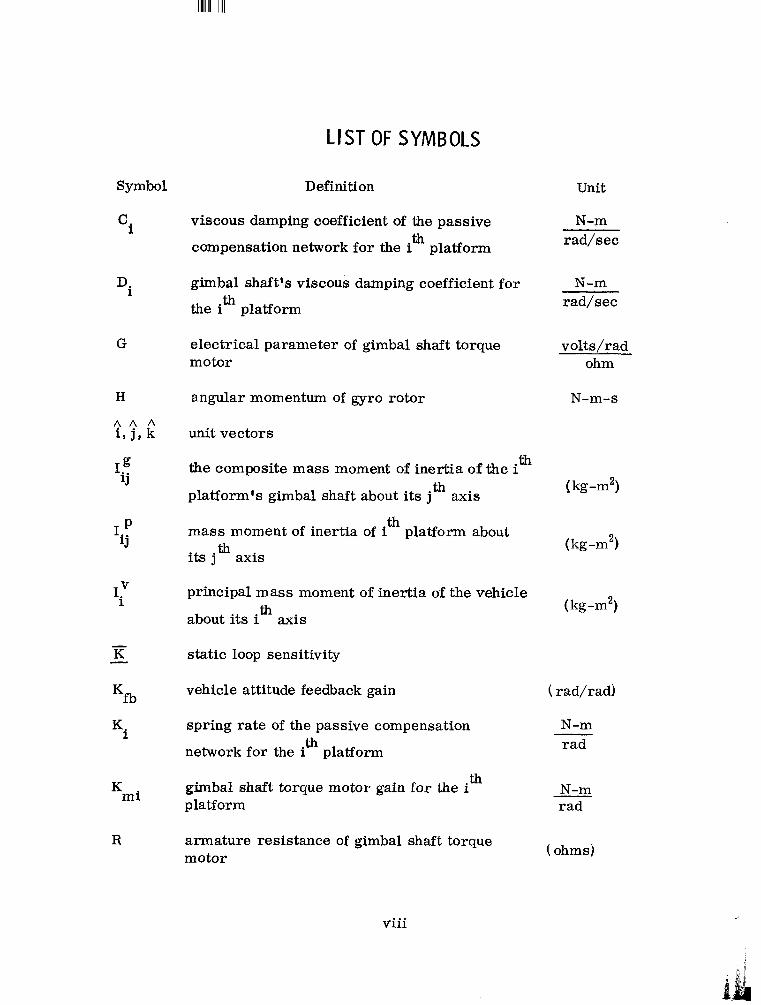
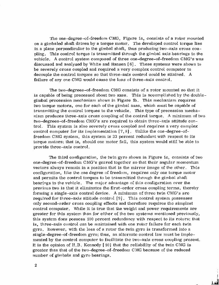
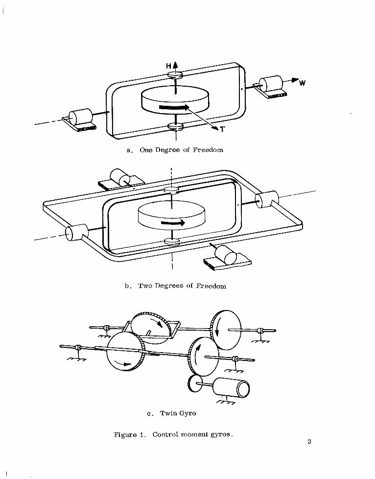
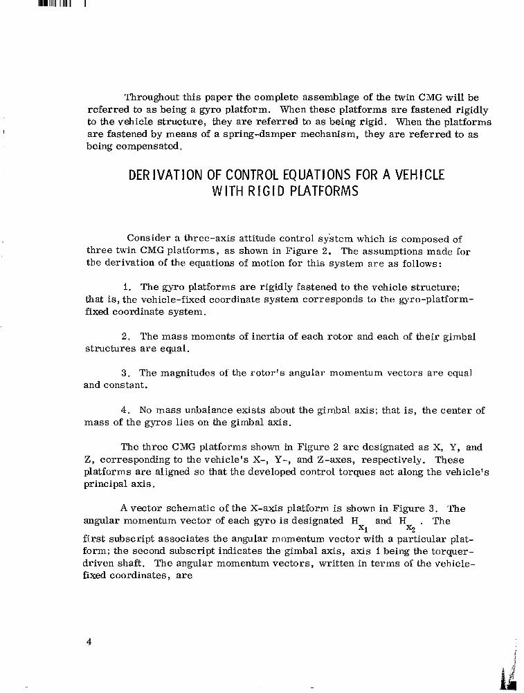
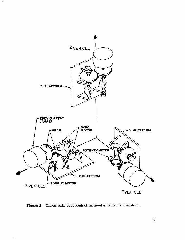
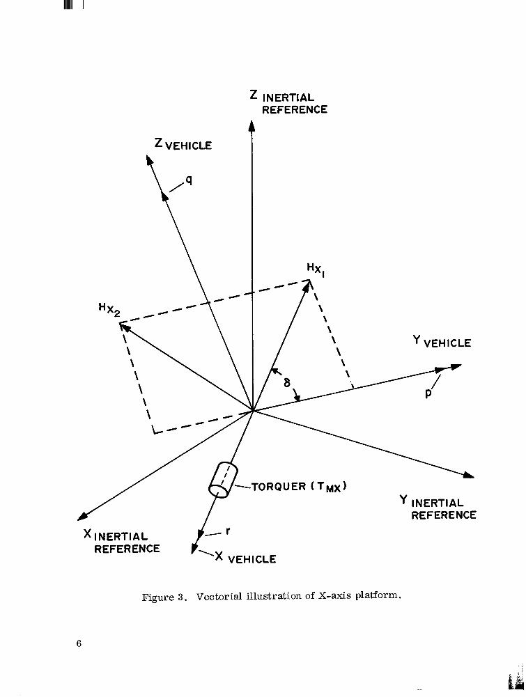
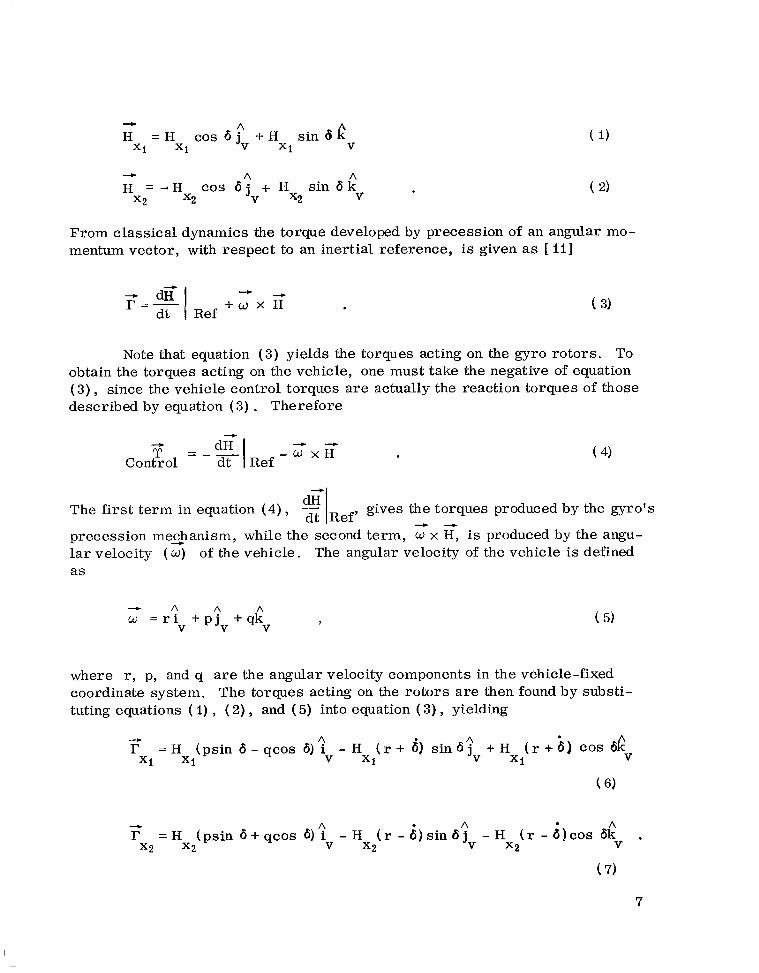
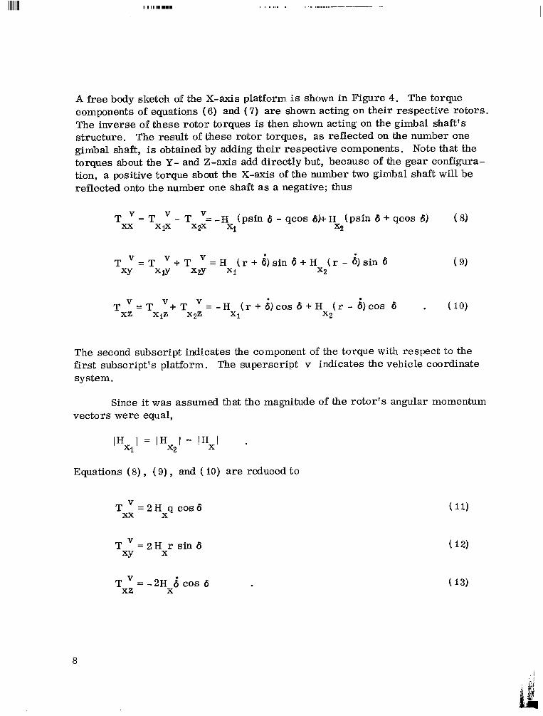
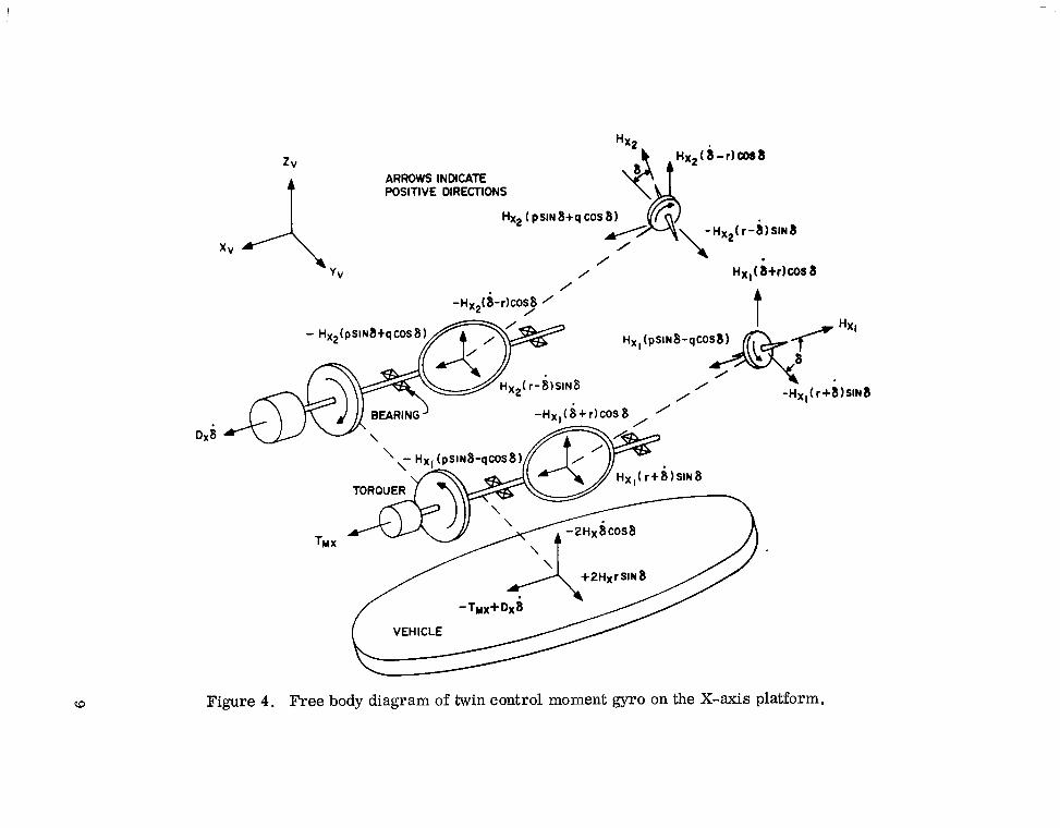
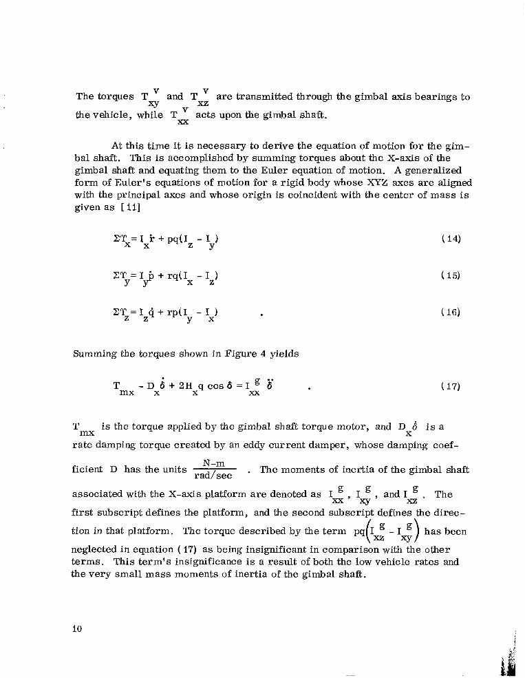
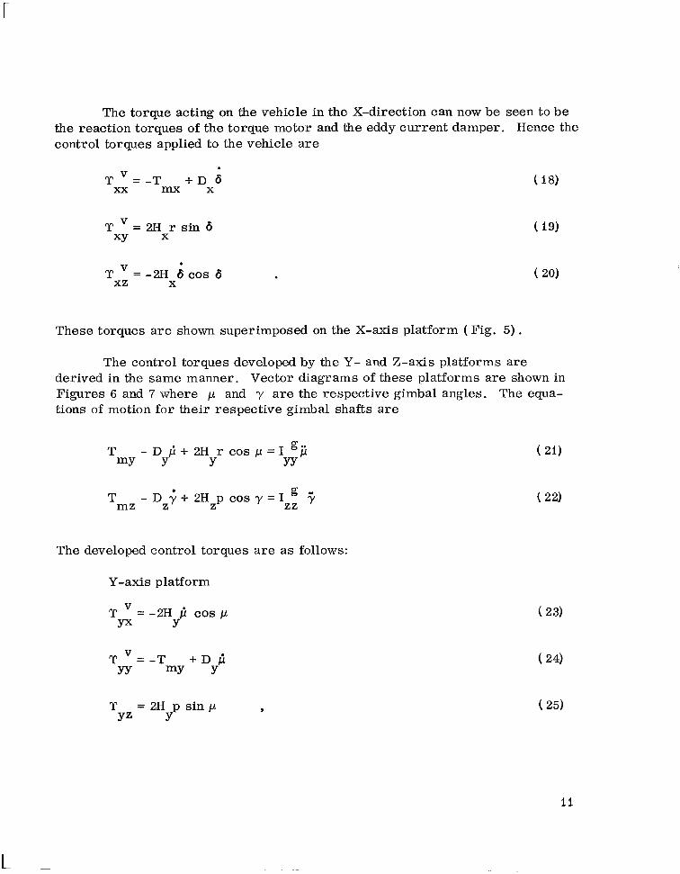
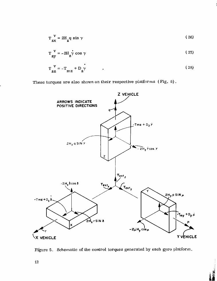
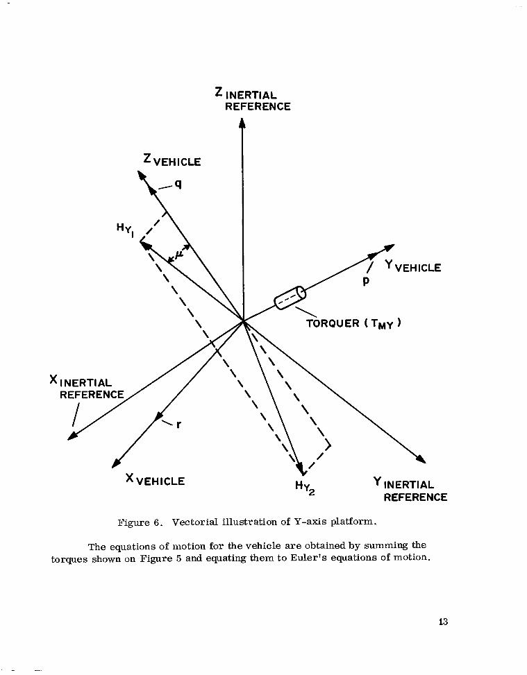
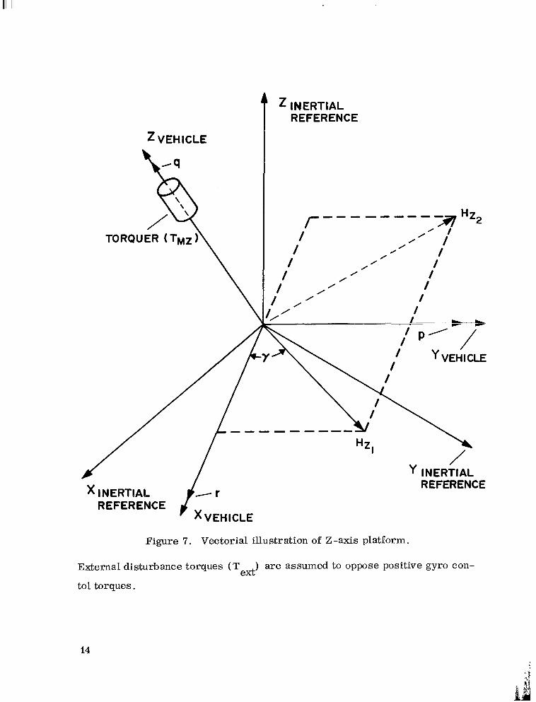
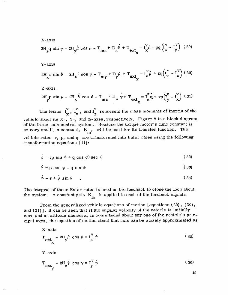
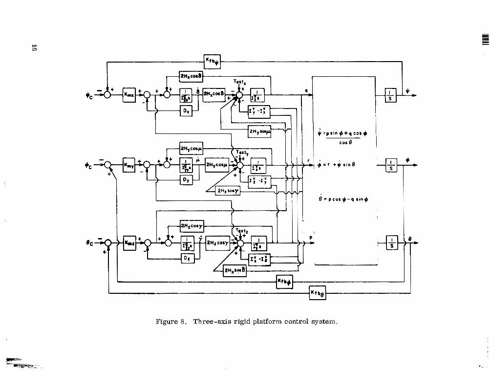
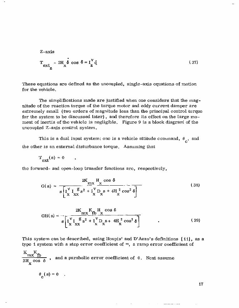
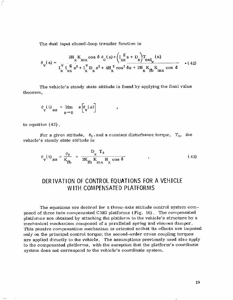
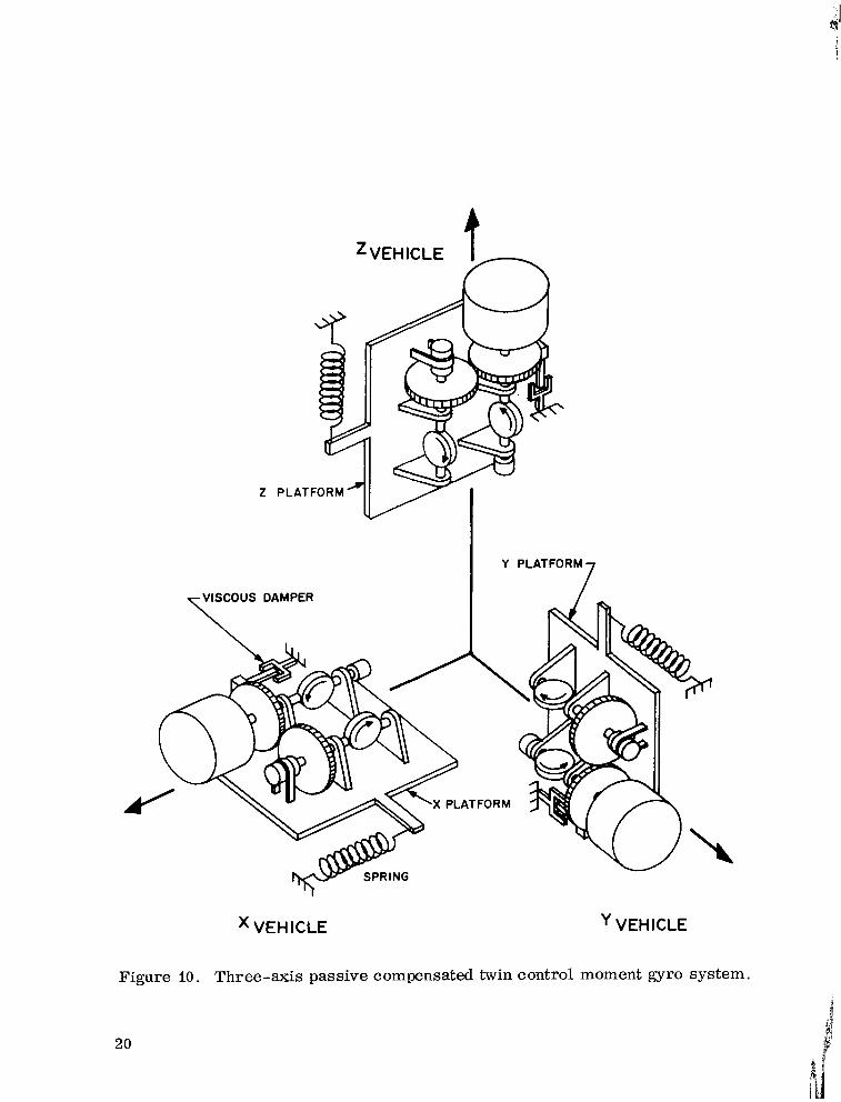
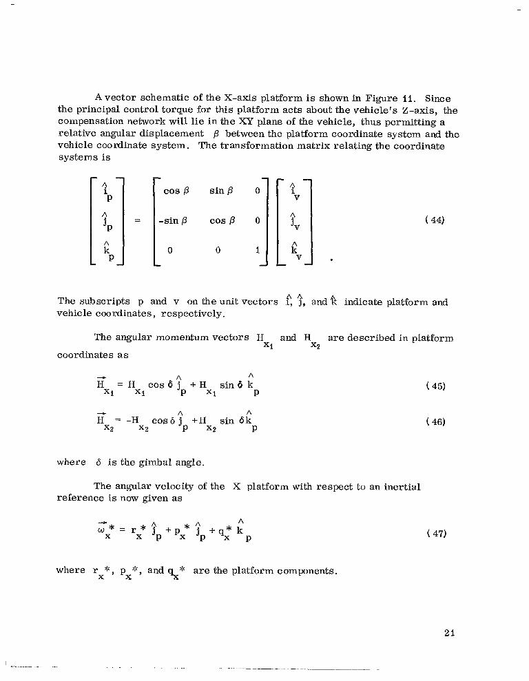
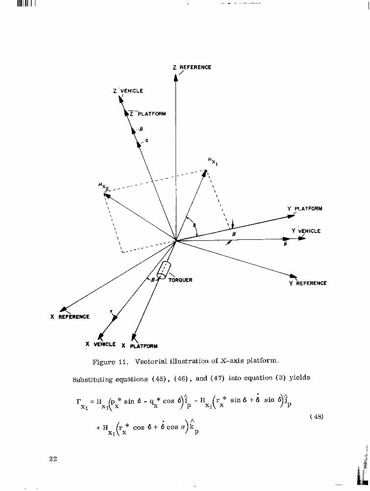
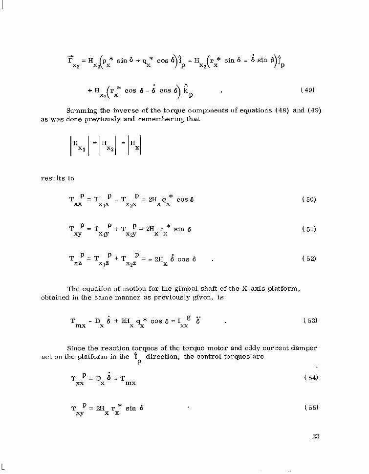
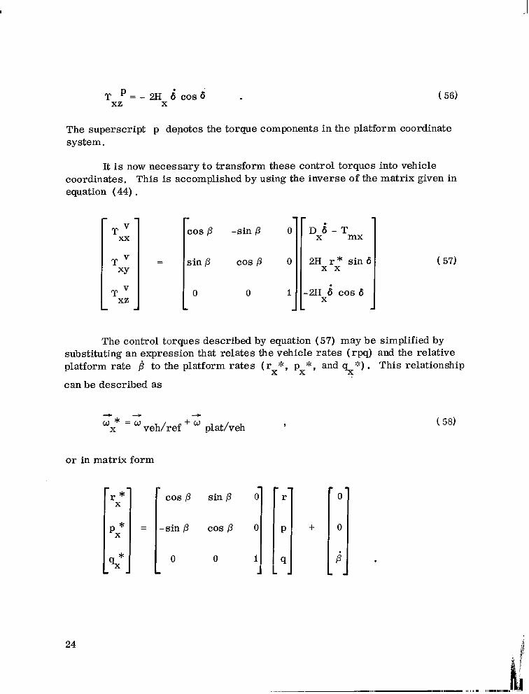
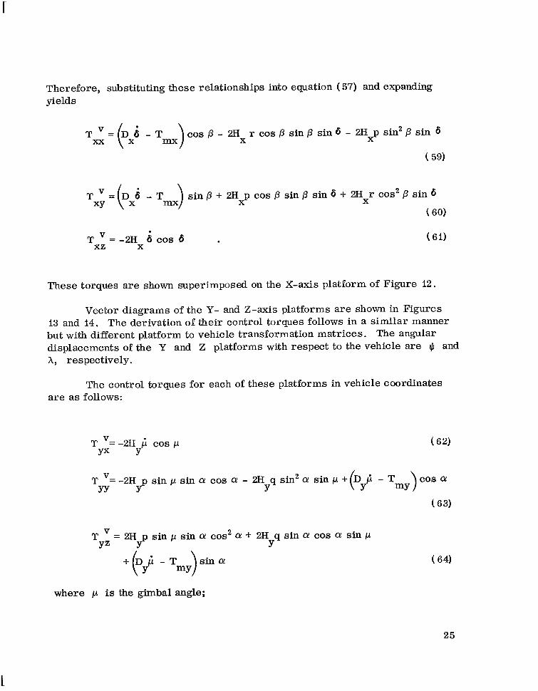
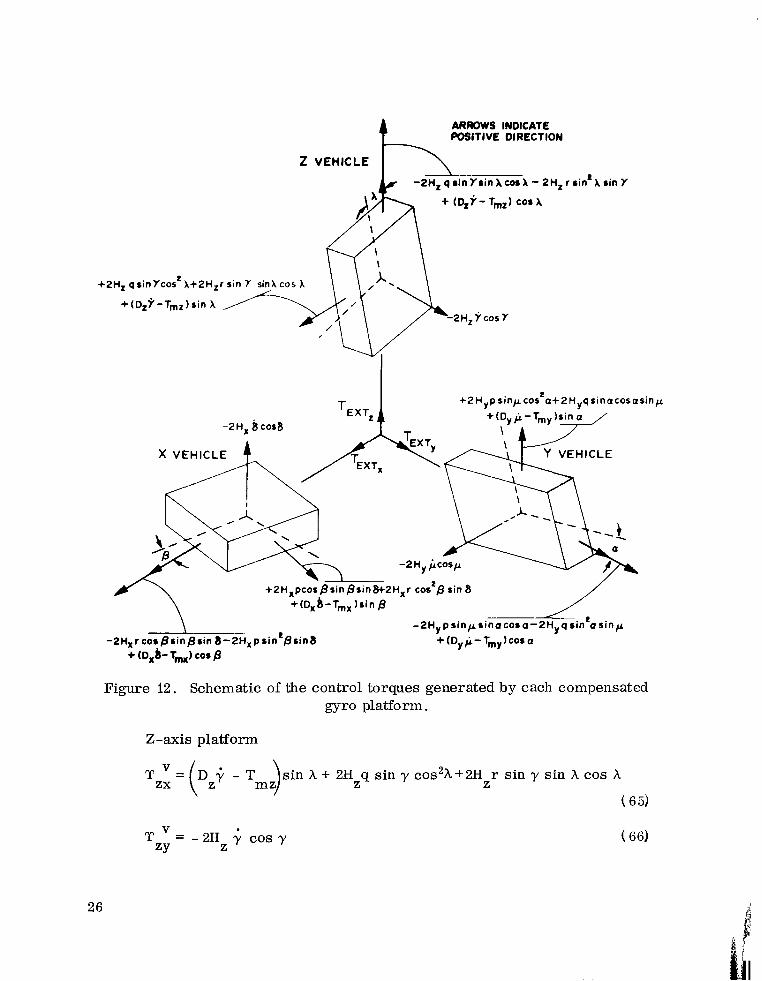
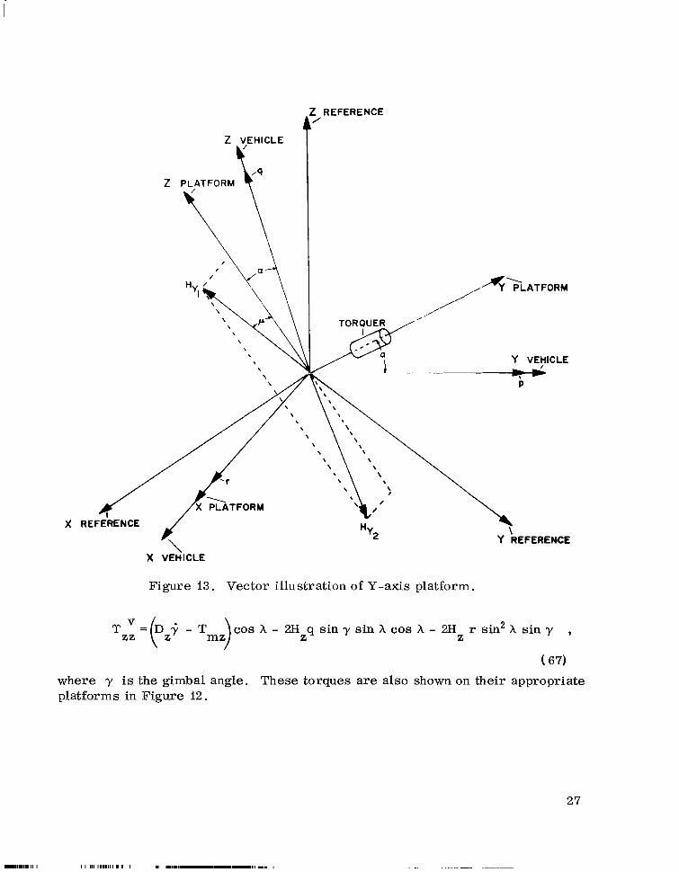
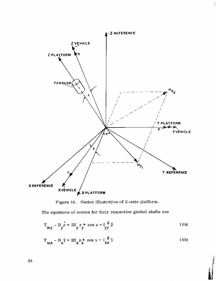
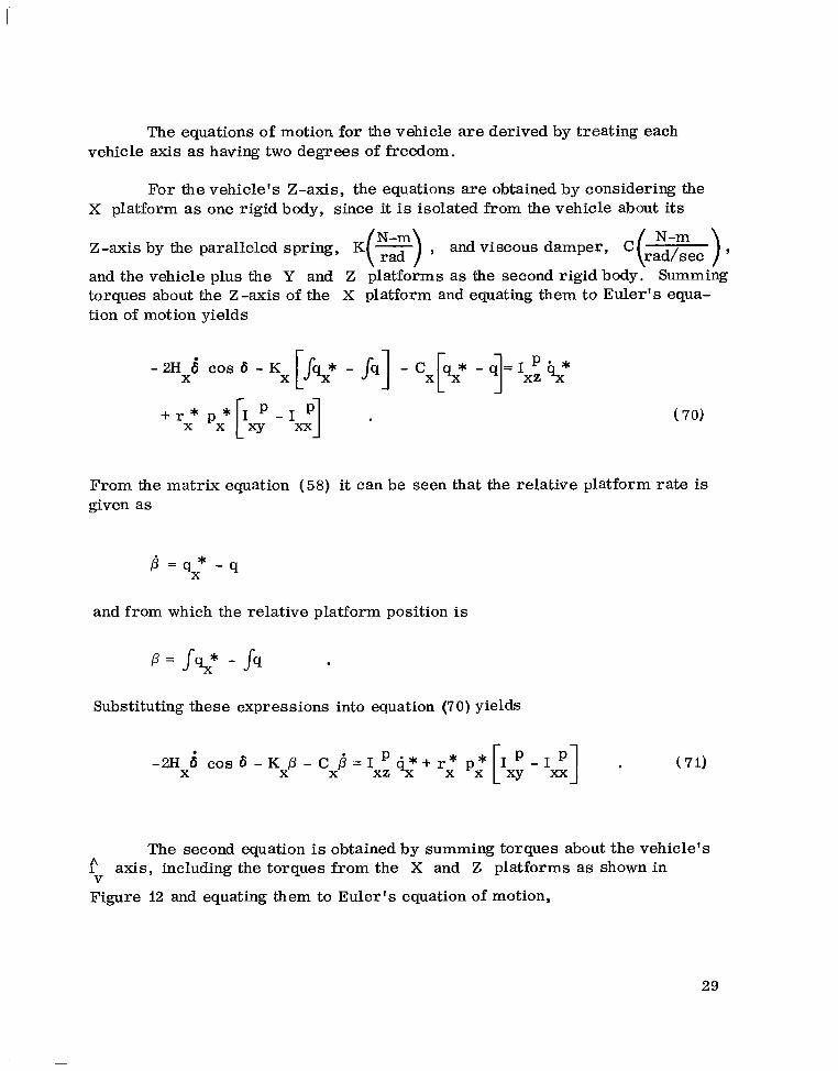
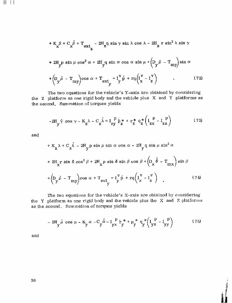
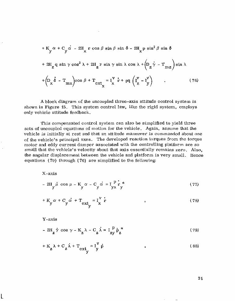
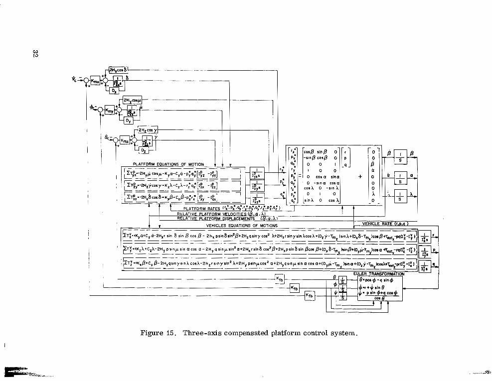
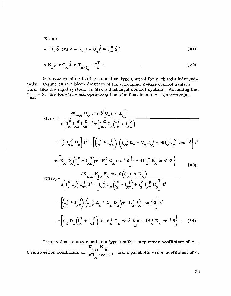
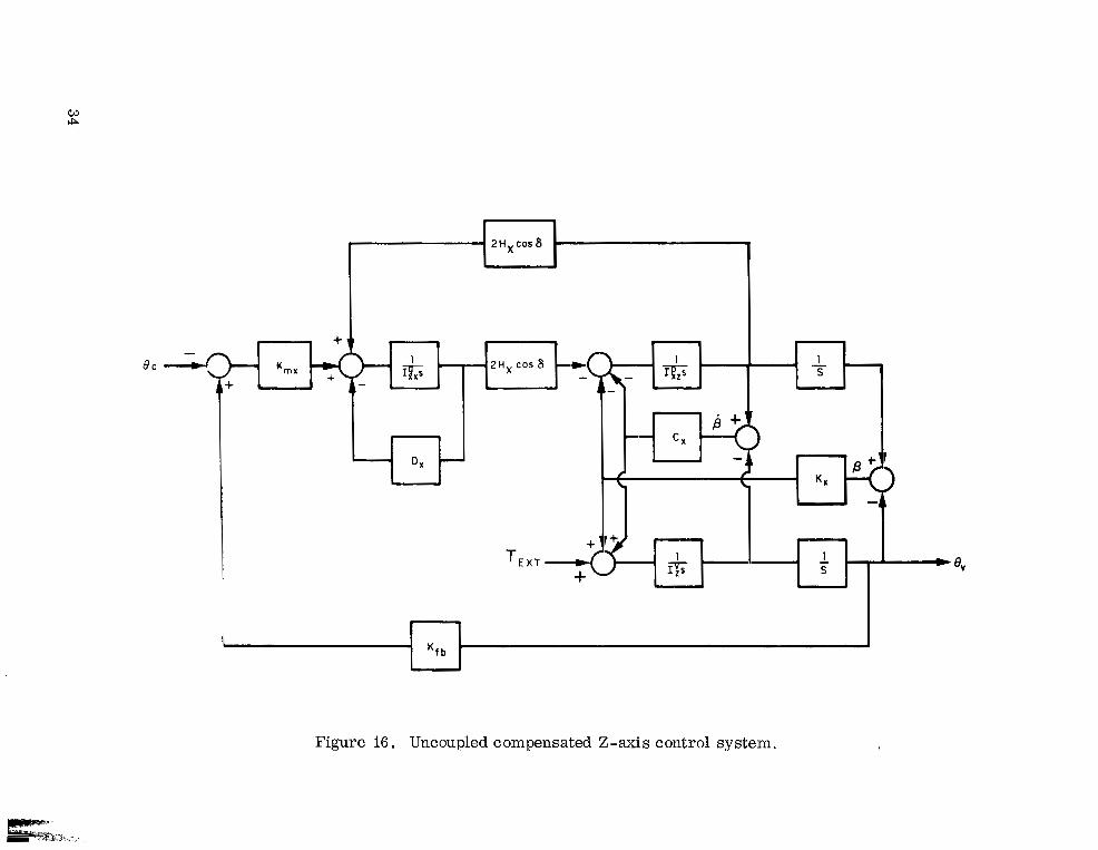
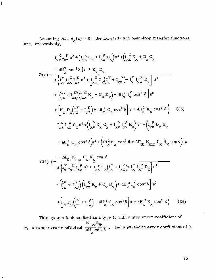
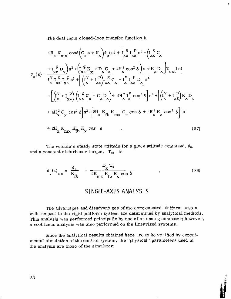
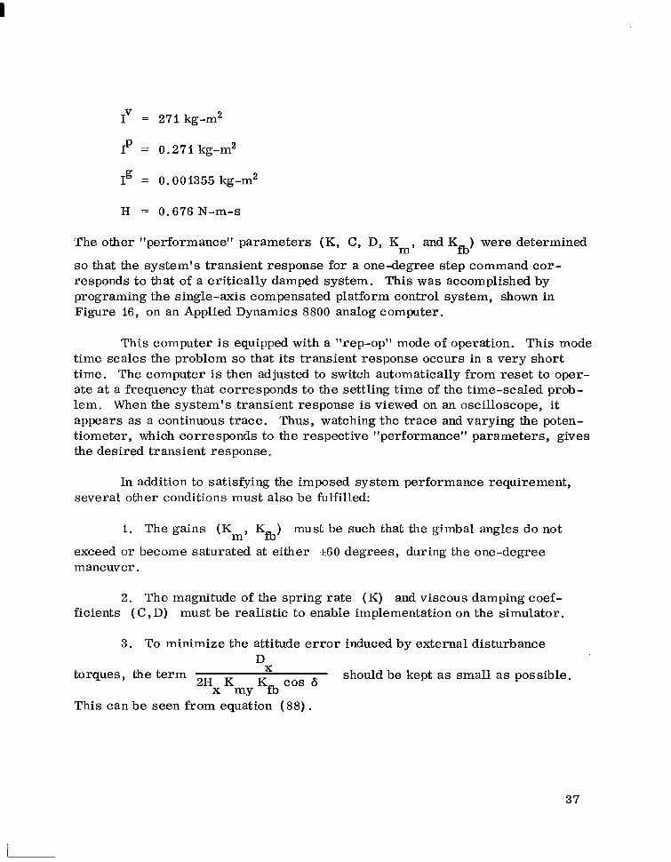
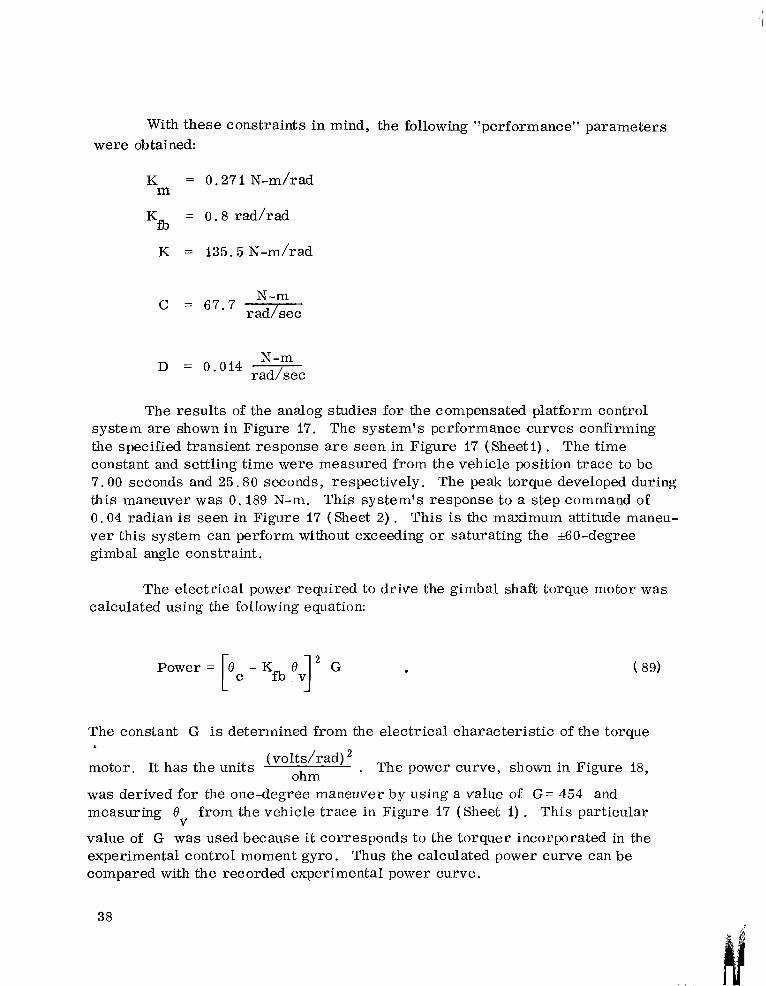
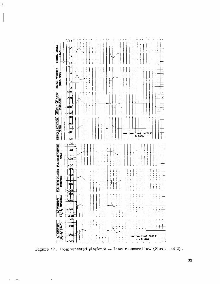
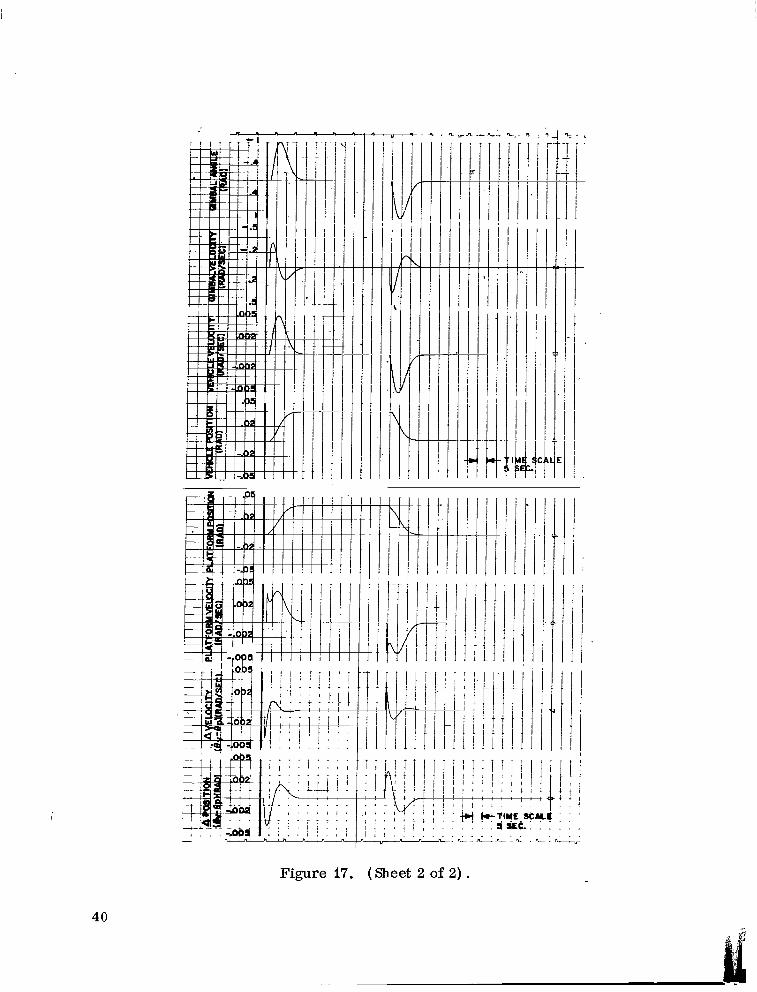
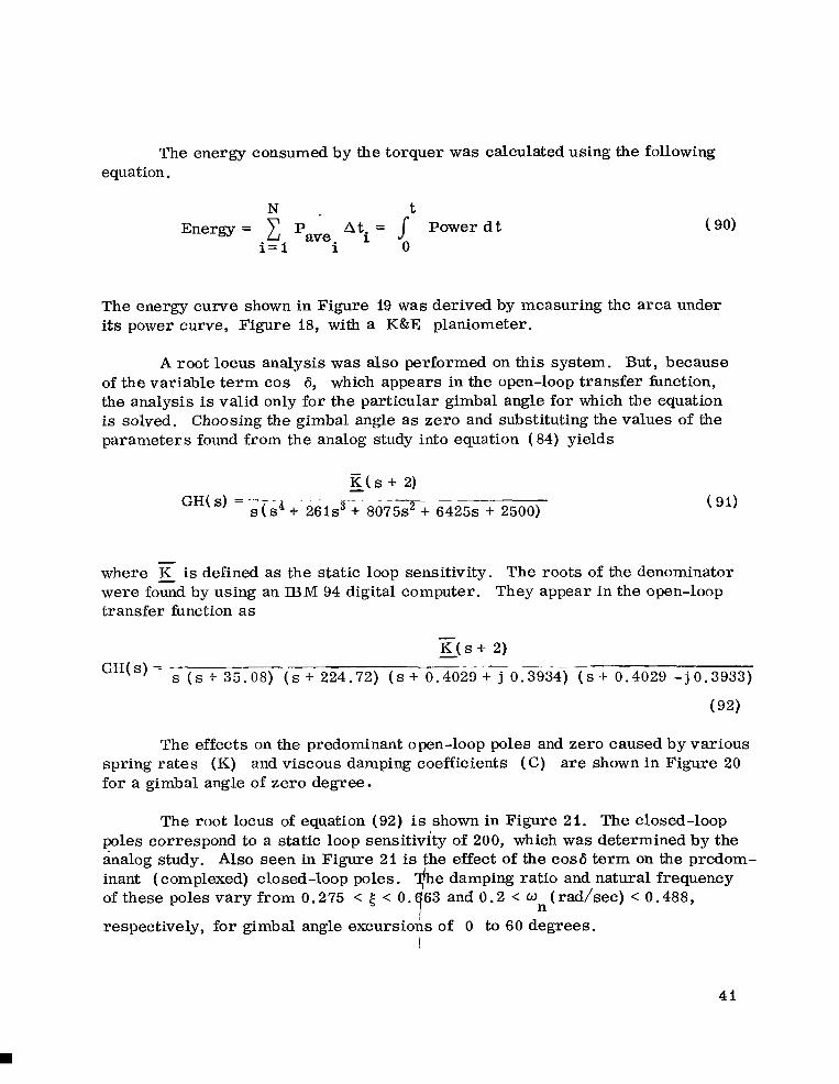
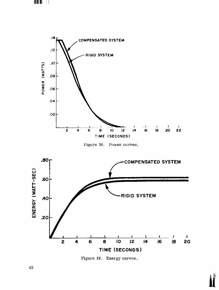
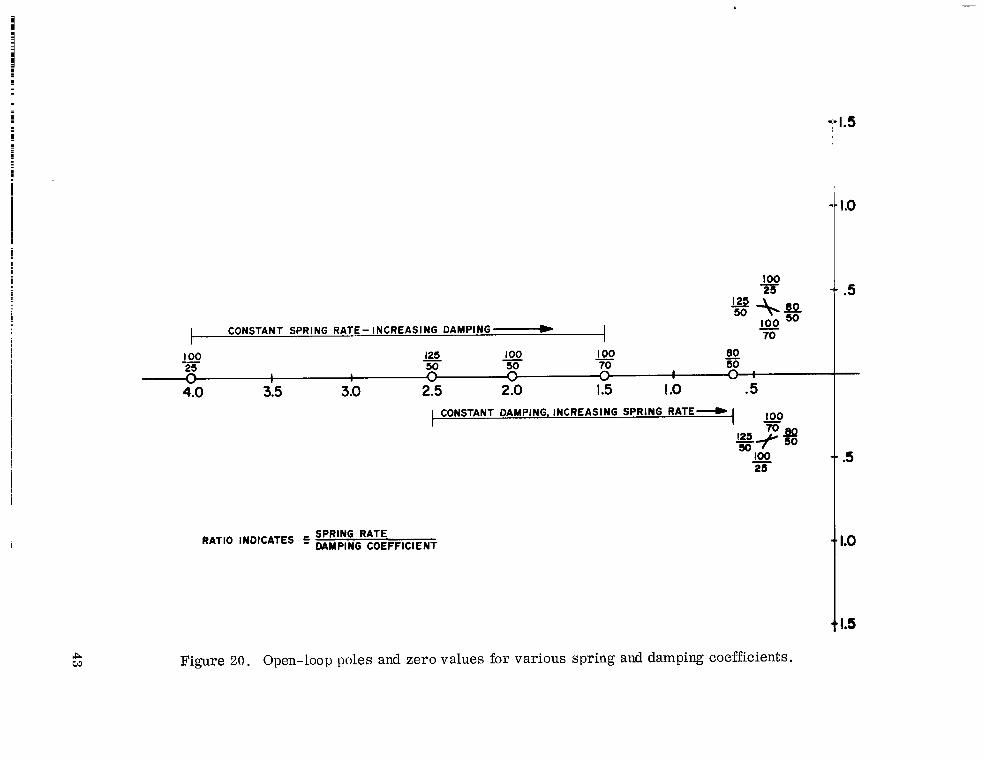
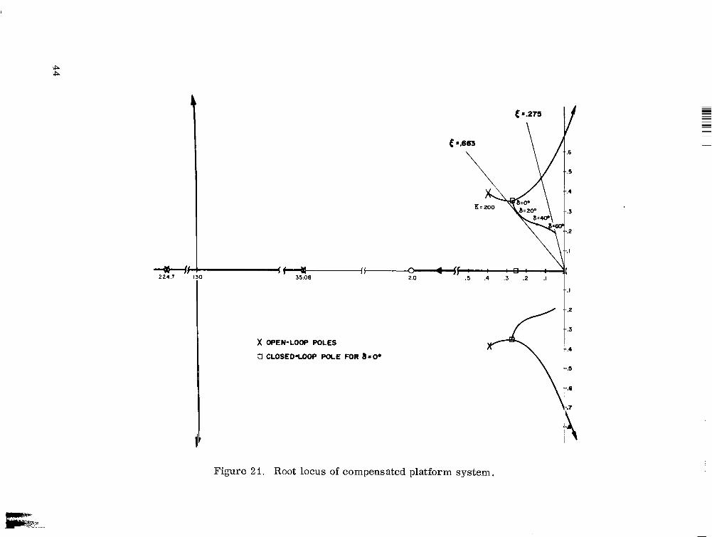
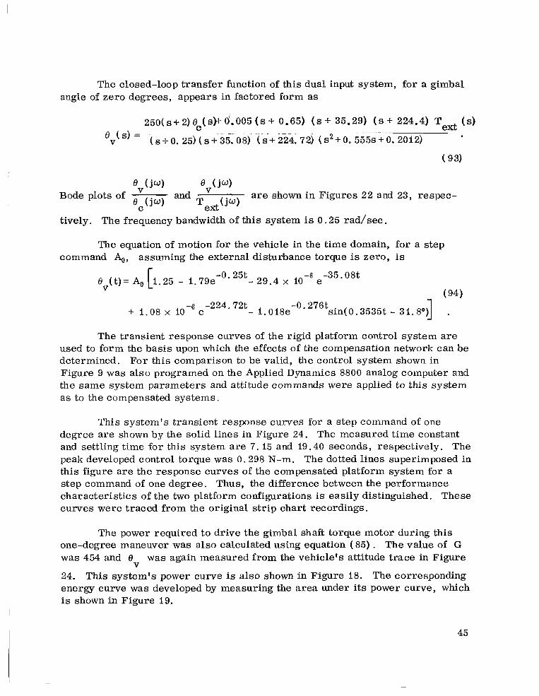
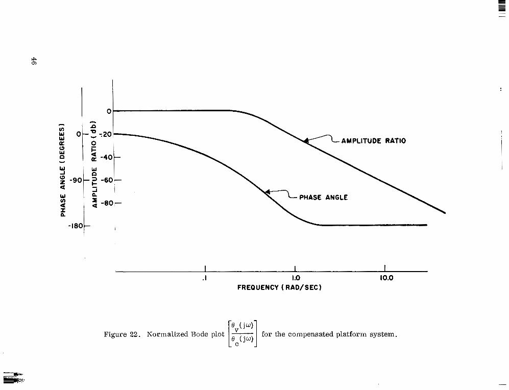
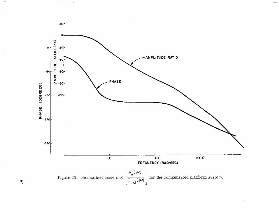
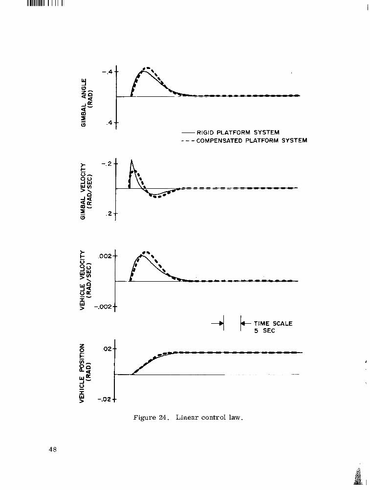
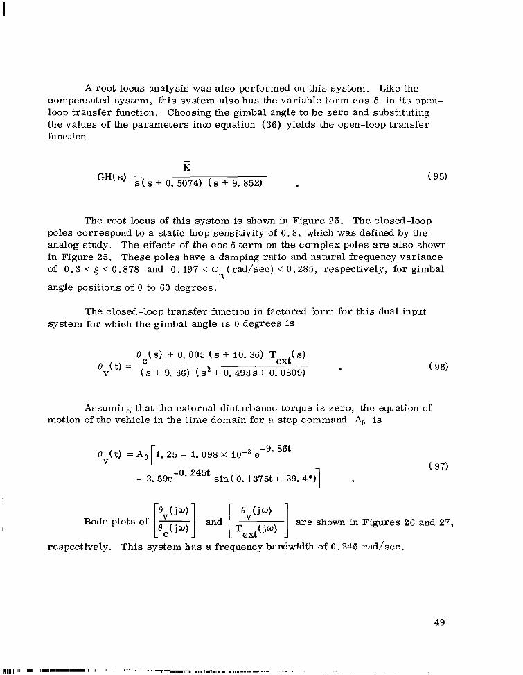
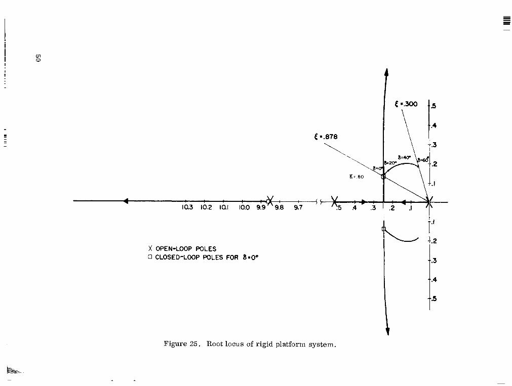
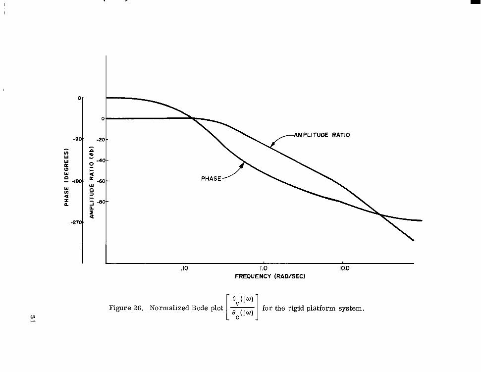
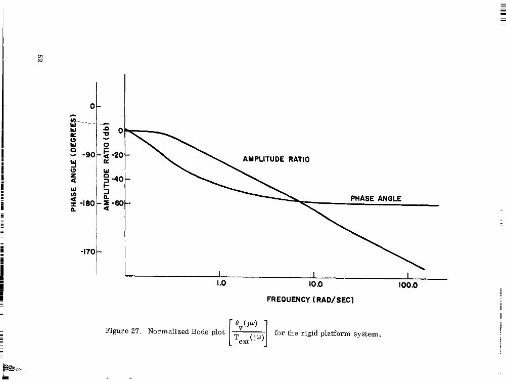
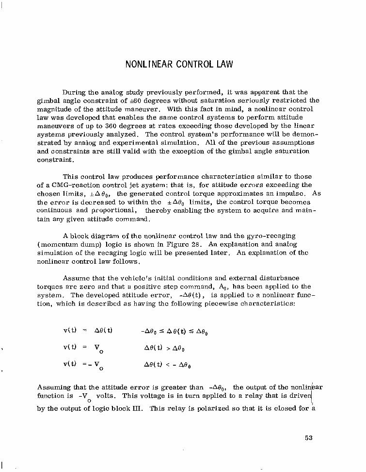
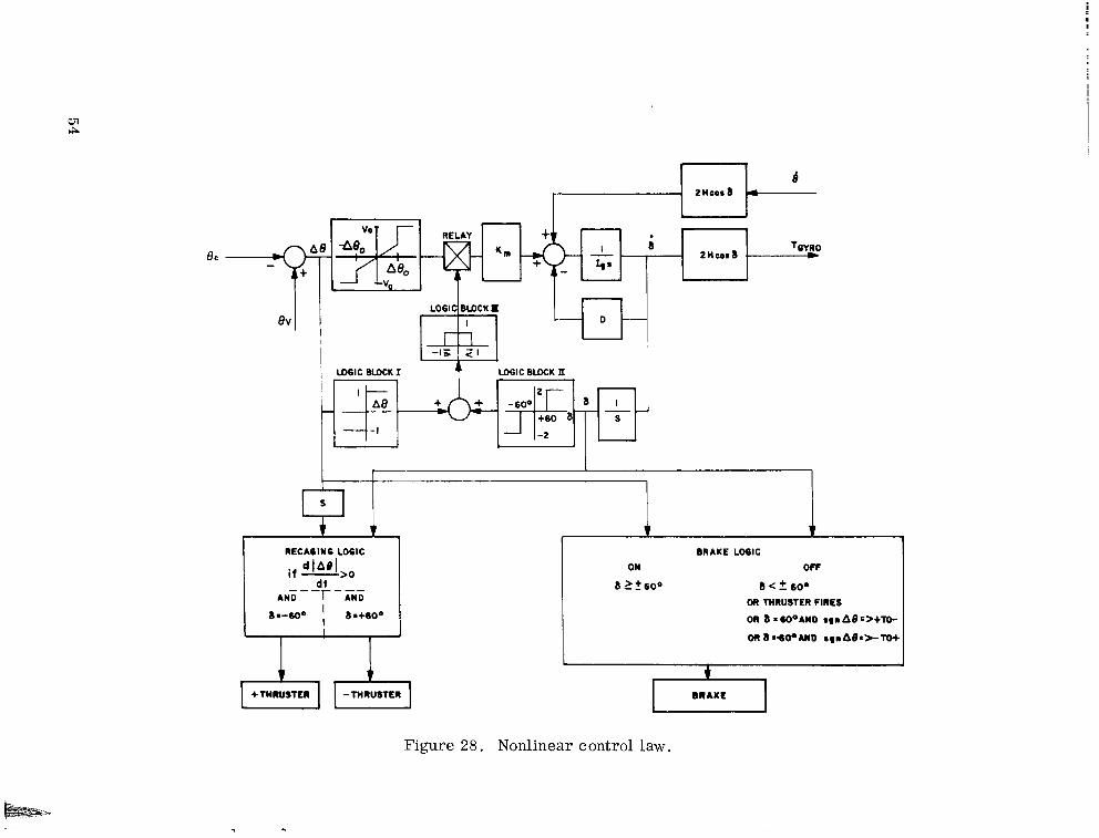
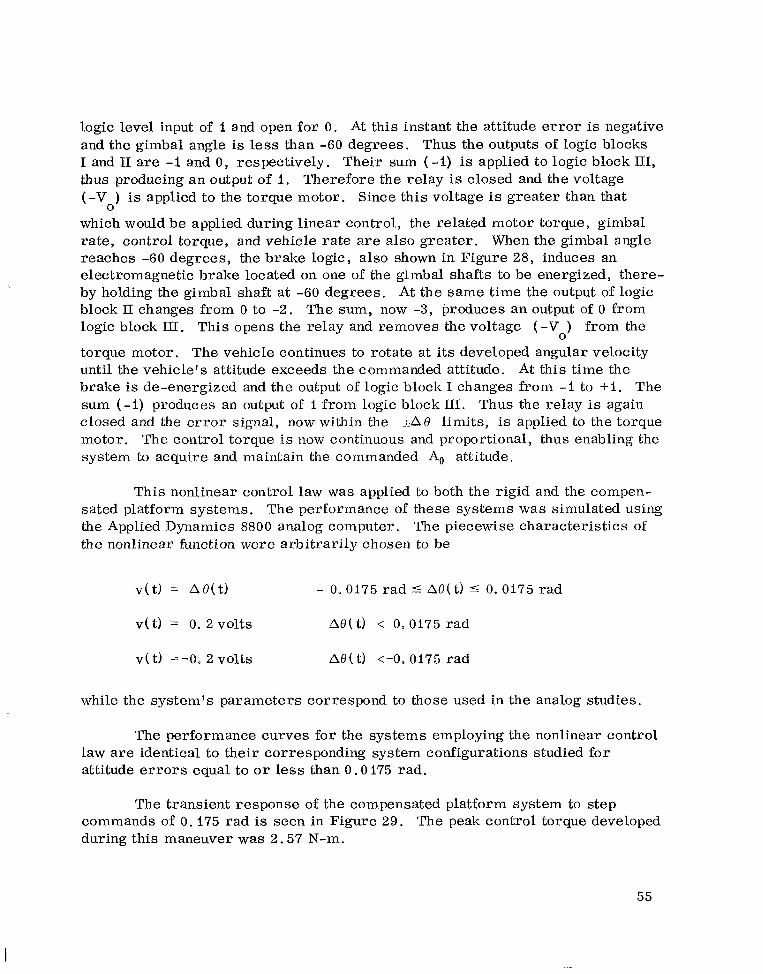
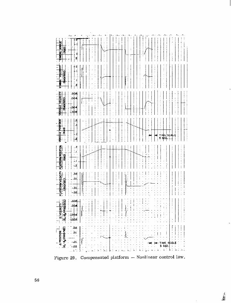
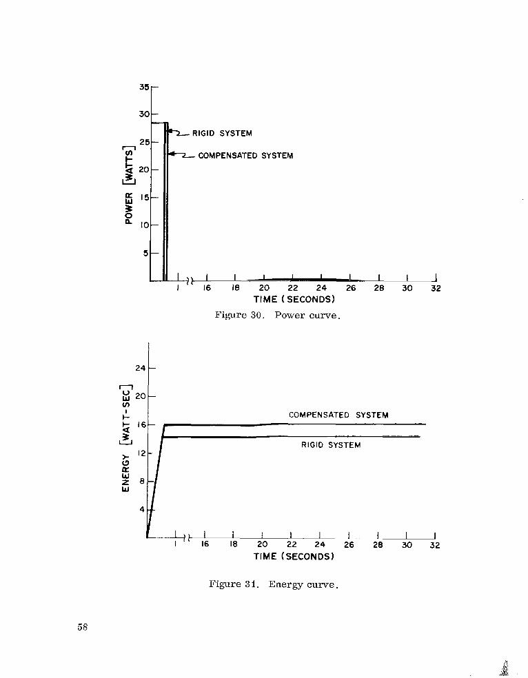
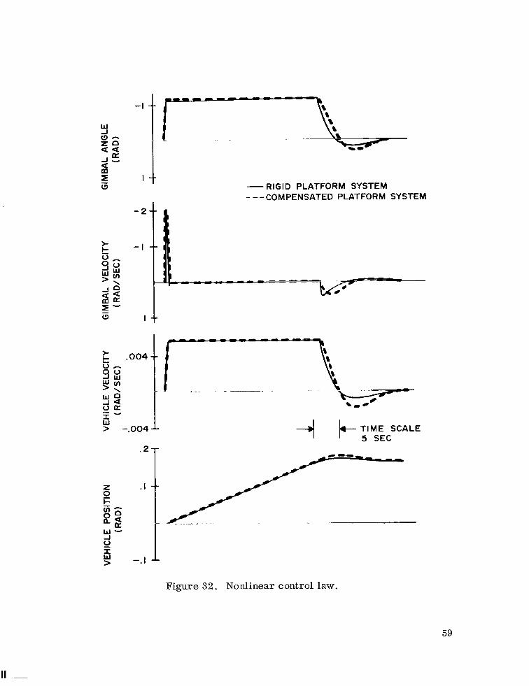
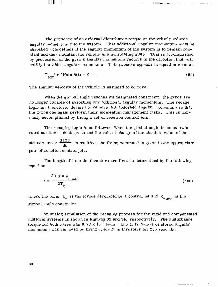
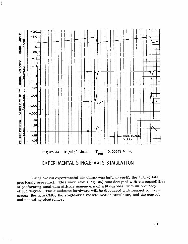
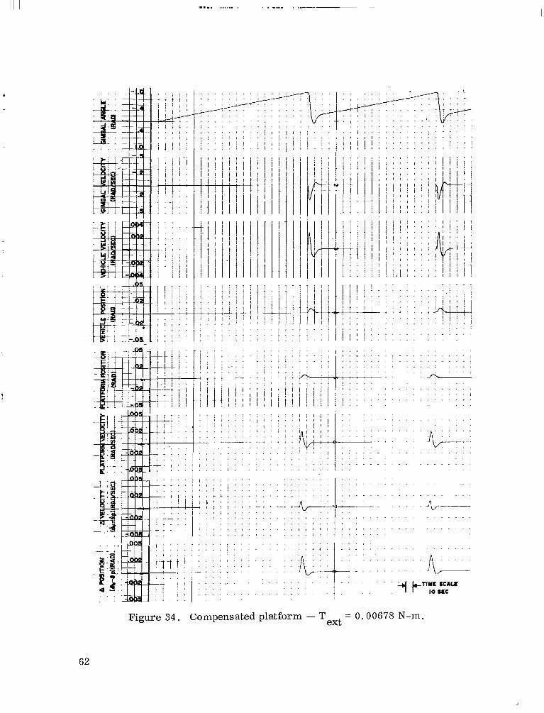
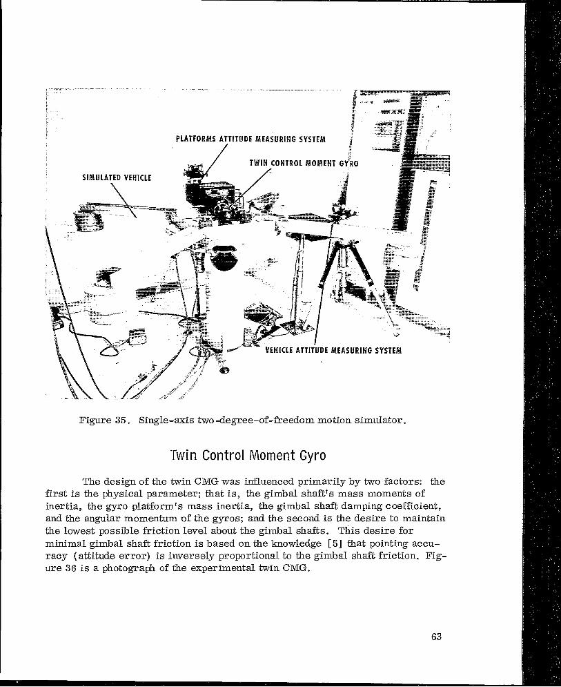
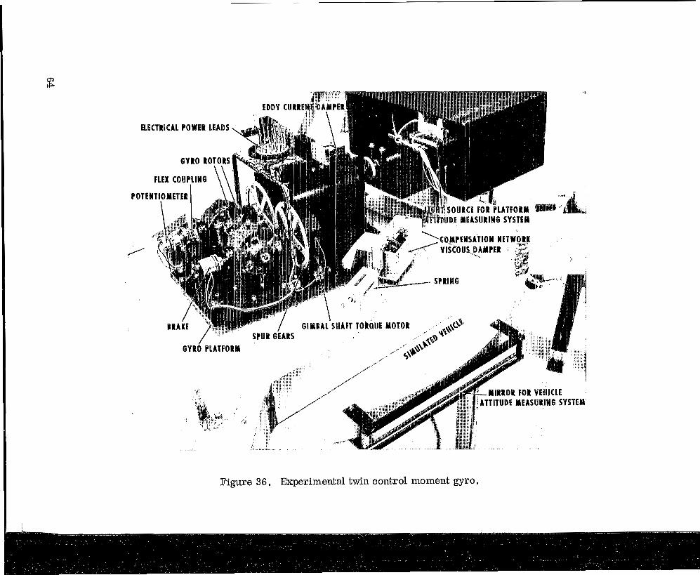
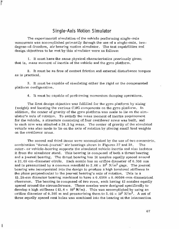
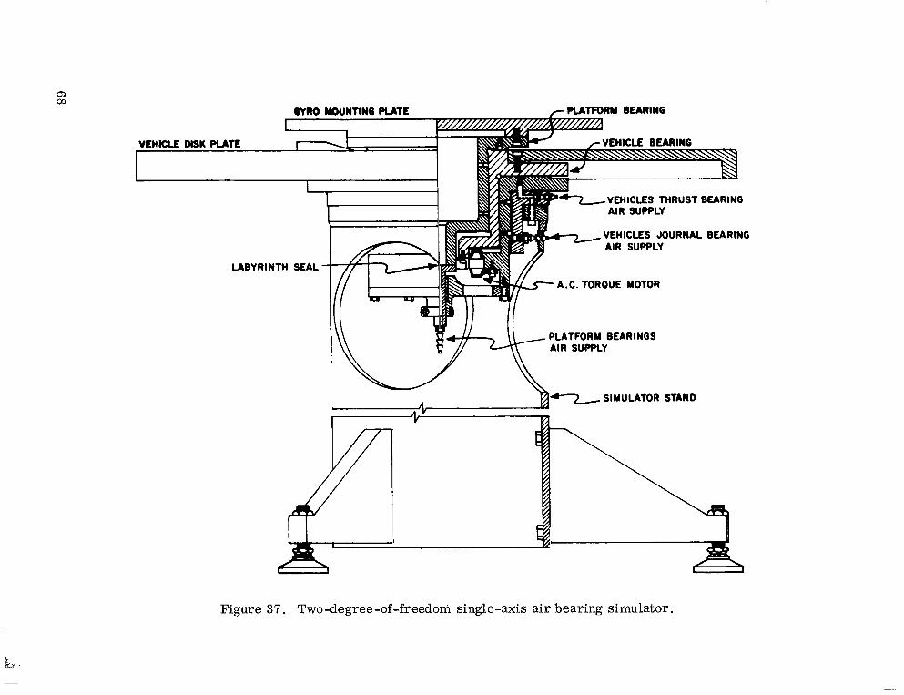
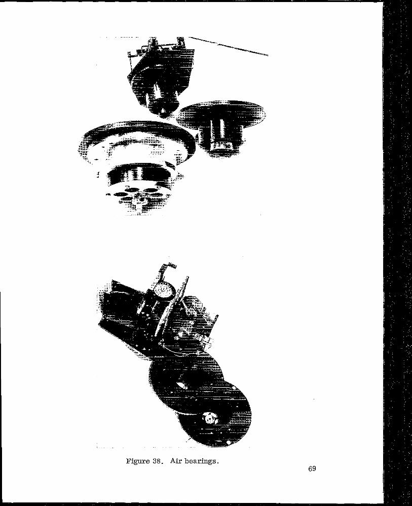
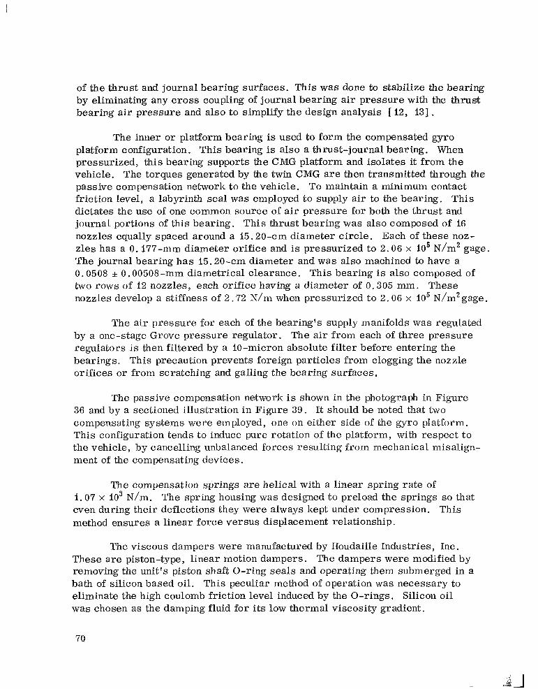
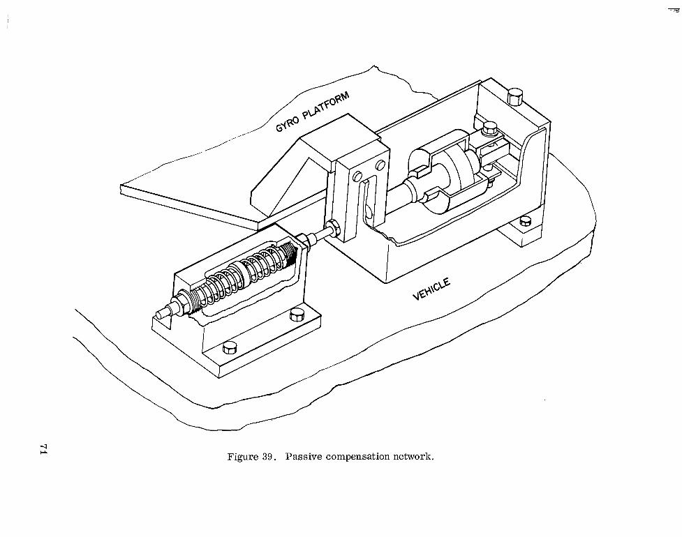
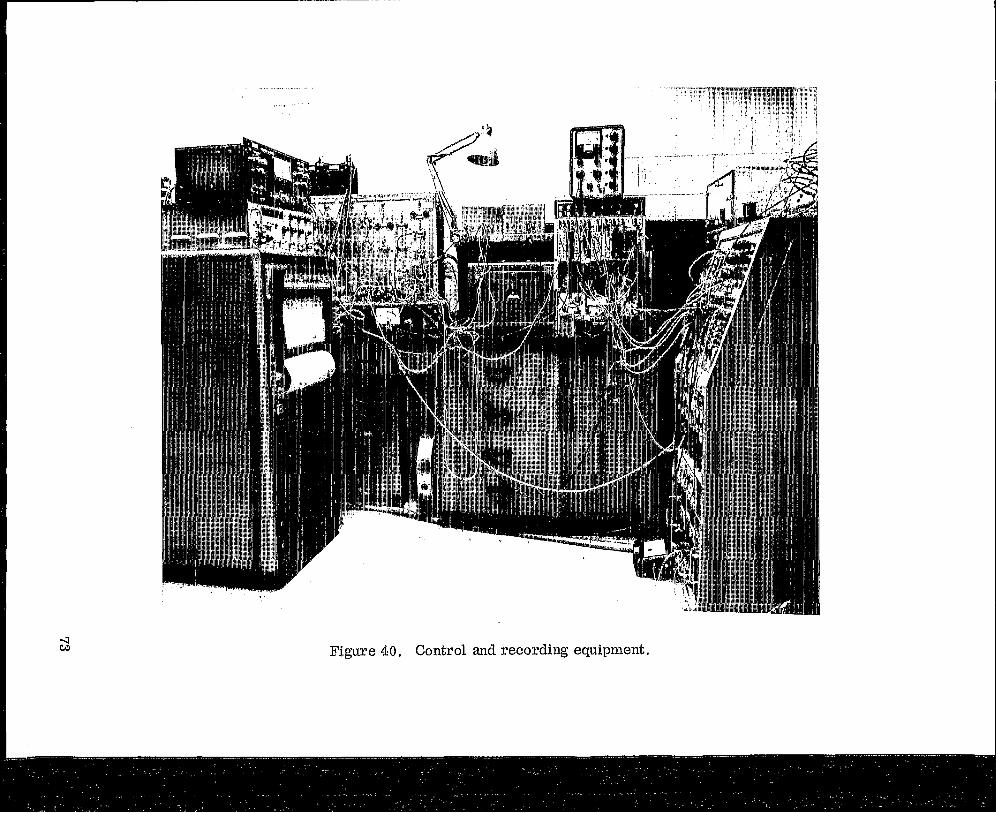
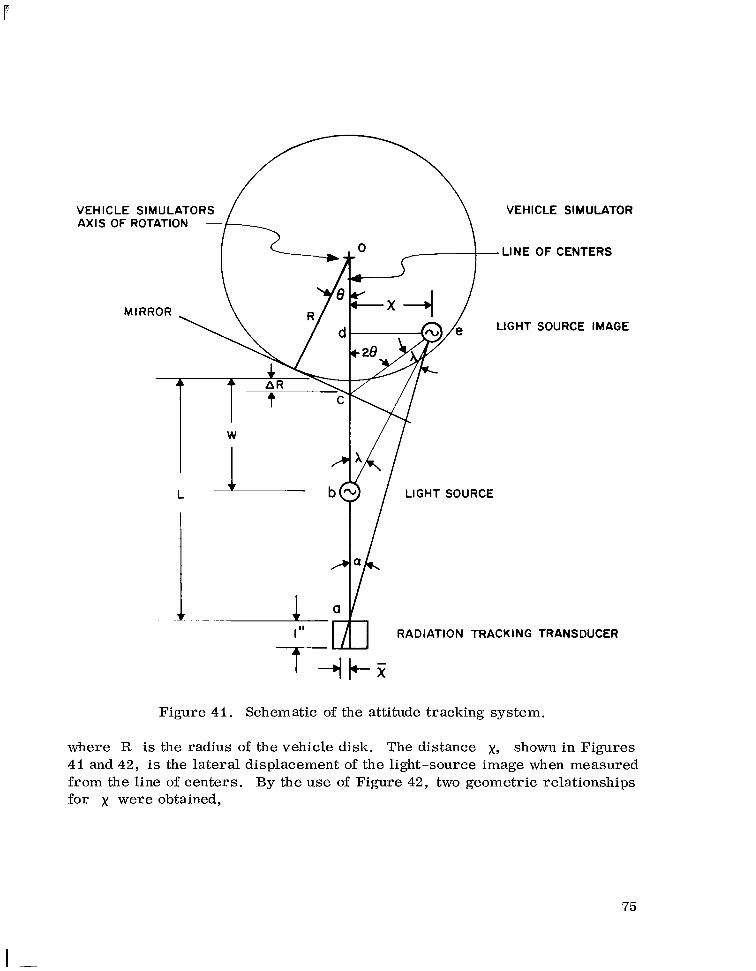
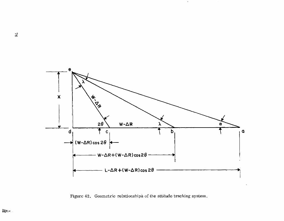
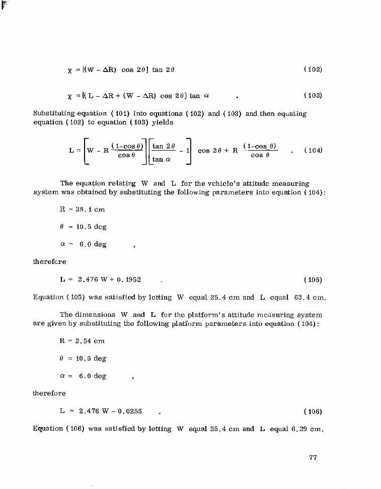
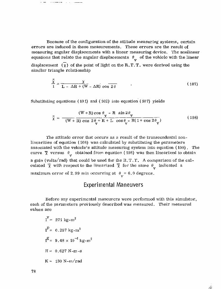
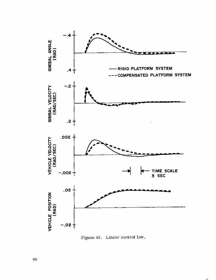
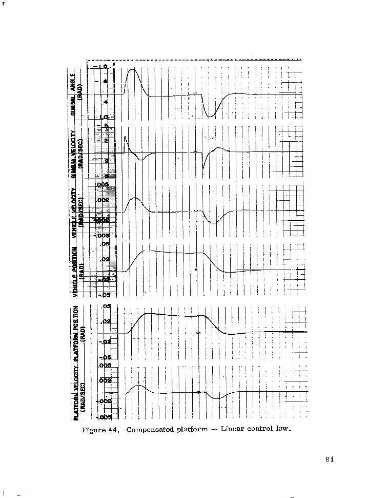
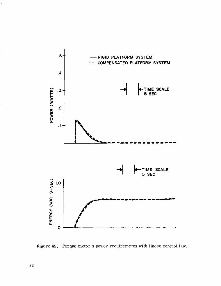
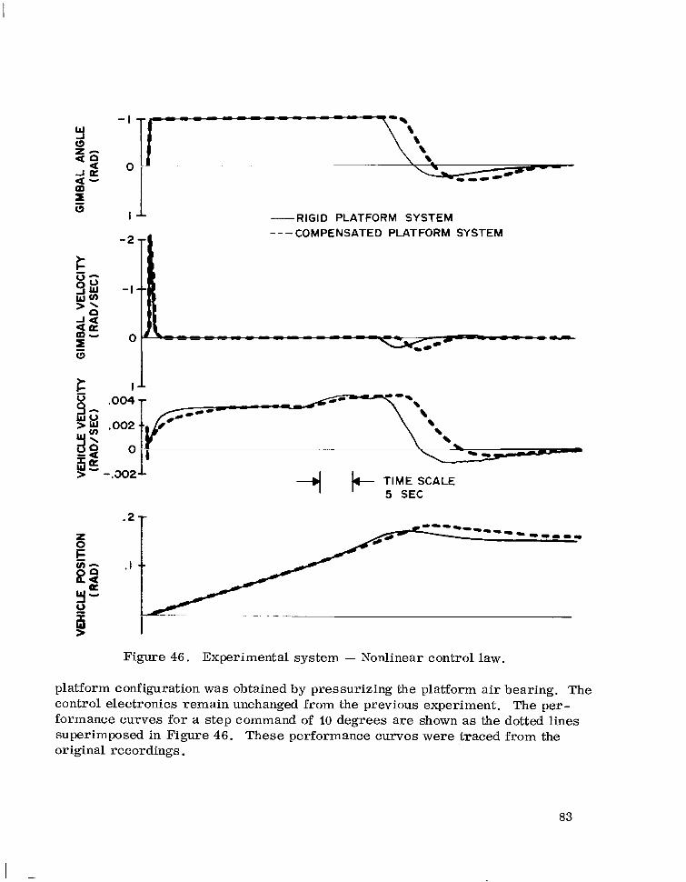
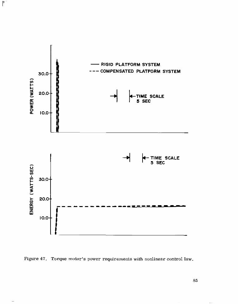

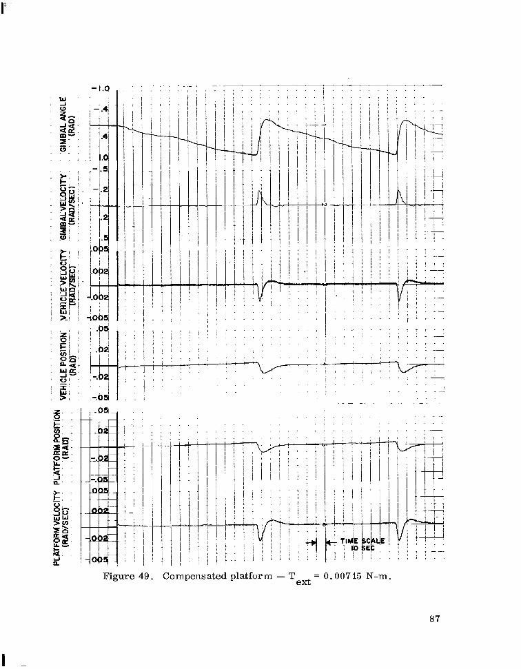
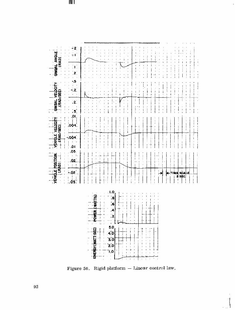
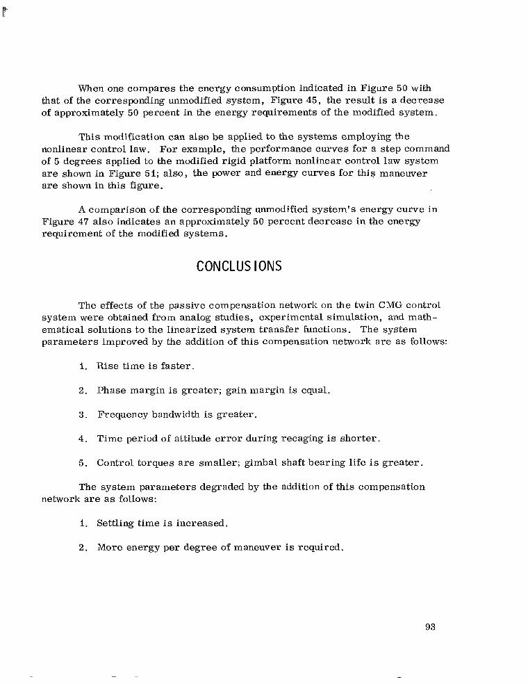
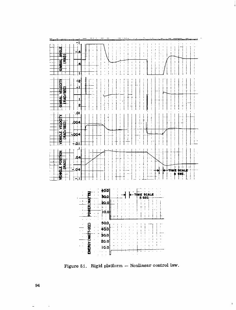


![Spartan Quark Gyro Installation Guide [Doc. v1.0]](https://static.documents.pub/doc/80x56/61fb1ed72e268c58cd5a6326/spartan-quark-gyro-installation-guide-doc-v10.jpg)


![Spartan Quark Gyro Installation Guide [Doc. v1.0] · PDF fileany size helicopter from tiny electric to the largest nitro helicopters. The holding ability of the gyro is excellent and](https://static.documents.pub/doc/80x56/5aa92c5d7f8b9a8b188c7c68/spartan-quark-gyro-installation-guide-doc-v10-size-helicopter-from-tiny-electric.jpg)


