NASA TECHNICAL NOTE - - - NASA TN D-4119 c, I A N EXPLICIT SOLUTION FOR THE LAGRANGE MULTIPLIERS ON THE SINGULAR SUBARC OF A N OPTIMAL TRAJECTORY by Rowland E. Burns George C. Marshdl1 Space Flight Center Huntsville, Ala. I NATIONAL AERONAUTICS AND SPACE ADMINISTRATION WASHINGTON, D. C. SEPTEMBER 1967 1 https://ntrs.nasa.gov/search.jsp?R=19670026339 2018-07-14T22:30:19+00:00Z
Transcript
N A S A T E C H N I C A L NOTE - - - N A S A TN D-4119 c, I
A N EXPLICIT SOLUTION FOR THE LAGRANGE MULTIPLIERS ON THE SINGULAR SUBARC OF A N OPTIMAL TRAJECTORY
by Rowland E. Burns
George C. Marshdl1 Space Flight Center Huntsville, Ala.
I N A T I O N A L AERONAUTICS A N D SPACE A D M I N I S T R A T I O N W A S H I N G T O N , D. C. SEPTEMBER 1 9 6 7 1
George C. M a r s h a l l Space Fl ight C e n t e r - Huntsvi l le , Ala.
NATIONAL AERONAUTICS AND SPACE ADMINISTRATION
For s o l e by the Clsoringhouse for Federal Scientific and Technical Information Springfield, Virginia 22151 - CFSTI price $3.00
LIST OF SYMBOLS (Cont'd)
Latin Symbols
X,Y,Z Cartesian coordinates
Y A general variable
Greek Symbols
Y Direction angle of rocket thrust
A
6
6.. 11
A
(T
Superscripts
T
N
A determinant
Direction angle of rocket thrust
Kronecker delta (6 . . = 0 if i f j : 6.. = 1 i f i = j )
If subscripted, one of three Lagrange multipliers: if not subscripted, the magnitude of the vector Lagrange multiplier A
11 11
Gravitational parameter of the attracting planet
Lagrange multiplier
Lagr ange mul tip1 i er
Denotes derivative with respect to time
Indicates the transpose of a vector or matrix
Indicates a matrix
Indicates a vector
Indicates a modified form of a quantity
V
1 I..
LIST OF SYMBOLS (Concluded)
Subscripts
Indicates an initial point ( t = t )
Indicates a final point ( t = tf)
Indicates the maximum value of a quantity
Indicates the minimum value of a quantity
0 0
f
max
min
i, j Summation indices
X,Y , Z Indicates a Cartesian component of some quantity
vi
I.
A N E X P L I C I T SOLUTION FOR THE LAGRANGE MULTIPLIERS ON THE SINGULAR SUBARC OF AN OPTIMAL TRAJECTORY
SUMMARY
The problem of optimal thrust programming of a single stage rocket- powered vehicle to achieve maximum payoff at specified end conditions is dis- cussed. gravitational field. The Lagrange multipliers are analytically determined for the so-called singular arc and the mass flow rate to maintain a singular a rc condition is derived. These Lagrange multipliers are directly related to the steering program by algebraic equations.
The vehicle is assumed to operate in vacuo in an inverse square
I NTRO DU CT I ON
An early problem posed by rocket technology to the mathematical disci- plines was the determination of the rocket trajectory which maximized the difference between the initial and final values of some function of the trajectory end points. This problem, first treated by the calculus of variations, has been the subject of numerous research papers.
A large amount of work was done in attempts to optimize the flight pro- file as a function of time under the assumption that the magnitude of the thrust w a s constant. direction of thrust as a function of time, but not the magnitude of thrust as a function of time.
I That is, the optimization was concerned only with determining the i
A s the theoretical developments became more sophisticated, the case of variable thrust magnitude was also treated. In this case, the thrust is assumed to be bounded between upper and lower limits; the lower limit may be zero (a coasting arc) but the upper limit is usually assumed to be finite so that the possibility of impulsive velocity change is excluded.
1
I
Concurrently with these efforts, work progressed in directions which may be regarded as perturbational effects of the basic problem. Such effects include aerodynamic drag, non-spherical gravitational fields, etc. These effects are not par t of the present study, and in this report the vehicle will be assumed to operate in vacuo over a spherical earth.
It is well known that if the formulation of the optimal trajectory problem allows variable thrusting maneuvers to occur , three types of subarcs , which are categorized by thrust level, may occur in the overall flight profile. The first possibility is arcs which have constant (non-zero) thrust levels over a non- zero portion of the trajectory. The second possible type of arc is the zero thrust arc. This possibility can be easily justified on an intuitive basis by considering an orbit transfer maneuver with a high thrust vehicle between widely separated orbits.
The third type of a r c is the so-called singular subarc of an optimal tra- jectory. This a r c occurs when the portion of the Hamiltonian which yields the direction or magnitude of thrust as a function of time (via Euler 's equations) vanishes identically. In this case, the thrust level is not immediately available from the Hamiltonian and further work must be done to determine the magnitude of thrust as a function of time.
A s long as the problem is formulated in the calculus of variations frame- work , Lagrange multipliers o r equivalent auxiliary variables must be intro- duced to determine the direction of thrust as a function of time. Much of the difficulty in the numerical calculation of optimal trajectories arises from the fact that the initial values of these Lagrange multipliers are not known and the resulting split boundary value problem requires repeated integrations of the equations which result from the theory. Any technique which solves analytically for the multipliers (hence, thrust direction) as a function of the state variables, time, and constants of integration would greatly reduce the labor and time involved in numerical isolations of optimal trajectories. tion of the three types of arcs which may occur along an optimal trajectory is particularly well suited to statements about which cases allow such an analytic solution of the Lagrange multipliers. The case of zero thrust is simplest, and yielded such a solution before the other types. several years [ 1 , 21 .*
The above classifica-
This solution has been known for
t W. E. Miner appears to be the first to have obtained this determination. The results of his work are reported in Aeroballistics Internal Note 20-63, Trans- formation of the A-Vector and Closed Form Solution of the A-Vector on Coast Arcs, George C. Marshall Space Flight Center, Huntsville, Alabama, 1963.
2
I
The case of constant (non-zero) thrust has not, as yet, been completely solved in the sense that is referred to here. A solution for three of six Lagrange multipliers in terms of state variables and constants of integration has been achieved through the use of a vectorial integral.
It is the third case that is treated in this paper. It is shown that for the case of the singular arc of an optimal. trajectory, a complete analytic solution for the steering program is possible. The solution is demonstrated in the form of three simultaneous algebraic equations. Subsidiary equations then yield the additional Lagrange multipliers in te rms of the solutions to these equations. Questions concerning the conditions under which these arcs actually do occur as segments of the trajectory are not discussed. siderations, the reader is referred to References 3 , 4 and 5.
For such con-
The analytic solution presented for the steering program is applicable to numerical trajectory calculations. necessary to integrate the differential equations which normally are used to calculate the Lagrange multipliers over that portion of the trajectory which fulfills the definition of a singular subarc.
Using these algebraic equations, it is not
FORMULATION OF THE PROBLEM
We wish to determine the extremumvalue of the difference between the initial and final values of some function of the end points, G. fuel expenditure is minimized if we choose G as the difference between the initial mass , m , and the final mass , m
0 f '
For example, the
i. e. ,
G = m - m 0 f '
In order to specify the constraints to which the rocket vehicle is subjected, w e w r i t e the rocket equation as
--c T A - v = - u - g m T
3
where
4
V = velocity
T = t h r u s t
m = mass
u = unit vector in the thrust direction
g = acceleration of gravity
A
T - The thrust, T, is assumed to satisfy the inequality
5 T 5 T min max
T
The velocity, is related "3 the posit-m vector, T, by
t - r = V .
Finally, the thrust, T, and mass flow rate, mc, are related by
T = - & c . (3)
Using the standard techniques of variational calculus, w e now introduce vector Lagrange multipliers and and a scalar multiplier cr to form the Lagrange fundamental function, F , as
4
The problem we now wish to examine is to determine the extremal values of
To initiate this study we first r e w r i t e F in the more tractable scalar nolation by introducing
4
= (x , y, 2)
A u = (cos y cos 6, s i n y cos 6 , sin 6) T
4
A where y and 6 are control angles (i. e. , direction angles of the vector u ) as shown in the figure below and subscripts indicate components, not partial derivatives.
T
5
We may now rewr i te F as
F = hi(Vx - T/,m cos 6 cos y + g 2 + h z ( t - T/m cos 6 s i n y + g ) Y Y
+ V3(h - Vz) + CJ(T/C + m) . (9)
The Euler-Lagrange equations, a necessary condition for an extrema1 path, are
%(%)-e = o
where the variables y. are V V , Vz, x, y, Z, y , 6, T, andm. 1 xs Y
Applying the Euler-Lagmnge equation to the variables V V , and V xs Y Z we have
hi + v i = 0
h2 + v2 = 0
h 3 + v 3 = O . (13)
Defining the ordered set (hi, Az, h3) as the vector AT and ( vi, vz, v3) as the -L
vector vT , we can write equations (11) , (12) , and (13) as
- 4
h + v = o .
6
Turning our attention to the variables (x, y, z) for the Euler-Lagrange equations, we find
These may be conveniently rewritten in matrix notation as
Using our Eevious notation for the vectors matrix by A": we have
and T, and abbreviating the
The Euler-Lagrange equation for variable y yields
T/m(AI cos 6 sin y - A2 cos 6 cos y) = 0 .
7
For a powered arc , T/m is not equal to zero. If w e assume that
we obtain
Similarly, for variable 6
T/m(hi sin 6 cos y + A2 sin 6 sin y - h3 cos 6) = 0 .
Again, for T/m f 0, we have
Ax hi cos y + h2 s i n y tan6 =
Eliminating y from this equation by use of equation ( 16) we obtain
f As t a n 6 =
It may now be seen that the variables y and 6 have been related to the Lagrange multipliers via equations (16) and (17) .
The Euler-Lagrange equation cannot be applied directly to variable T, since T enters linearly. Writing the equation for F as
8
(where h has been written for dhf + A$ + Ai )we see that F can become independent of T for certain situations; namely, i f the coefficient of T vanishes
If the coefficient of T vanishes, the value of T becomes indeterminate and we may wri te (at the moment) only that T is bounded within the physical limits of the problem, i. e. ,
T s T 5 T min max
The sign ambiguity in the expression a/c r A/m = 0 can be resolved by the Weierstrass test. Originally
tan y = hz/hl
so that
f hi cos y = QT$-
and
with
sign (cos y ) = sign (sin y ) .
Then
f As tan 6 =
9
'\,
. , t
giving
sign (tan 6) = sign (cos y ) .
Then
J T q hf + A$ + A3
cos 6 = f
and
with
sign (cos 6) = sign (s in 6) .
In order to pursue the question of sign choice further, w e may w r i t e F as
F = A i ( V x + g,) + A2(+ + g ) + A3(+ z z + g ) + v i ( k - VX’ Y Y
+ v2(9 - v ) + V S ( i - VZ) + am Y
+ T[ a/m - l /m (hi cos 6 COS y + & cos 6 sin y + h3 sin 6) 3 .
The Weierstrass condition now requires that for a minimum the function
- F(t, Y, 9) E = (t, y, 9, y8, 9:;:) = F(t, Y:;:, i z : )
10
be positive for all sets y"' sufficiently near y and for all sets y . member of this equation vanishes under consideration of the strong variations of the controls y and 6 since i, and 6 do not appear. Thus
The last
For y. f y and y. Z 6 we have 1 1
c
yi = Y l
so that
T/m(Al cos 6 cos y + h2 cos 6 s i n y + A3 sin 6)
w e have
cos 6 ( A l c o s y + & s h y ) 2 0 .
Then
cos 6 (* djhf + h i ) 2 0
111l1l1lll Ill 111l11111ll111111111111lllllllllllllll1lll111 Ill Ill1 I1 IIIII I II
or
sign = sign cos 6 .
Choosing
gives
Ai cos 6 c o s y + A z cos 6 siny + A 3 s i n 6 2 0
o r
then
Our function F now becomes
and the condition for the singular arc is
a/c - A/m = 0 .
12
The remaining sign ambiguity, f m, corresponds to the physical choice of initial firing direction. Further discussions will be restricted to the case of the singular arc.
This cannot be expected to be a result of mathematics.
O u r final variable, m, gives the equation
& - T/m2(Al cos 6 cos y + & cos 6 sin y + A3 sin 6 ) = 0 .
Again, expressing y and 6 in terms of AI, A2, and A3 we have
b =F T/m2 A = 0
which becomes - by our discussion of sign choice
b - T / m 2 A = 0 .
Before proceeding to the solution for the multipliers, we note that from equation ( 14)
t - .. A = - v
so that equation ( 15) may be written
The matrix x" is too general for our purposes. We specify a Keplerian field
13
where 1.1 is the gravitational parameter MG, i. e. , the mass of the attracting i planet multiplied by the universal gravitational constant. From this definition
6.. 3x.x. ( i , j = i , 2 , 3 )
where
x. = x o r y o r z 1
r has been written for dx? + y2 + 22
6.. is the Kronecker delta. 1J - .b -c
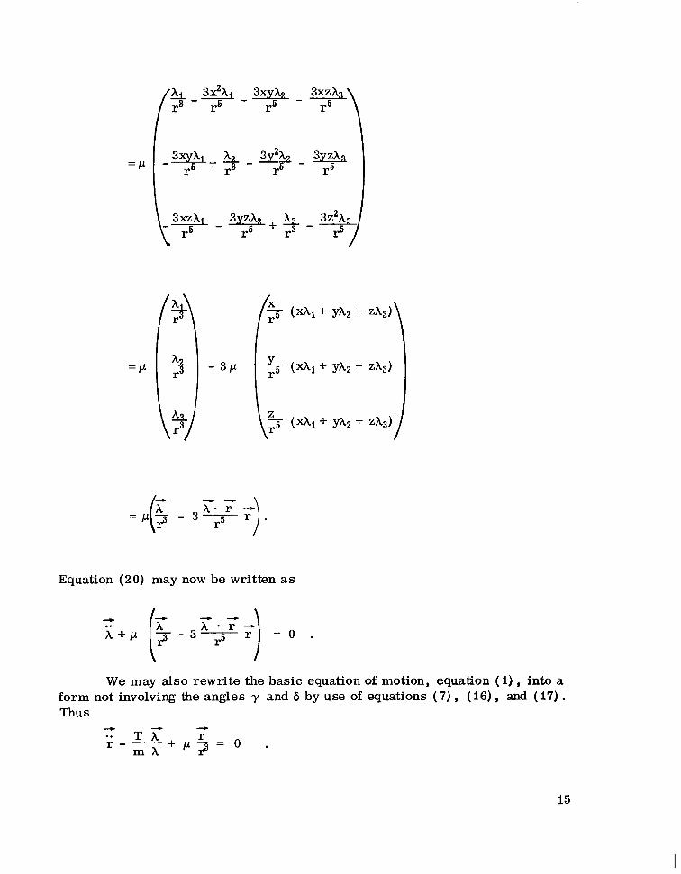
We can now w r i t e the expression A"A under the Keplerian field assump- N d
tion, A A , as
p-+ 3 x2 -3Ewry r5 9
-3pyz r5 9
14
Equation (20) may now be written as
We may also rewrite the basic equation of motion, equation (I), into a form not involving the angles y and 6 by use of equations (7), (16), and (17) . Thus
15
, . . . . . .. . .. . ._ -. . . ... .. . .. .-
The principal results of this section may now be summarized as
4
T C r - .. r - - - + p - - - O , m h 2 -
a h C M
- - = o . -
Equation (24) specifies that we remain on a singular arc .
Before proceeding to the integration of this system of equations, it is worthwhile to consider the following. In equation (21) we have three position and three velocity components which must be initially specified.+ Innequations (22) and (23) we must specify the initial values of the vectors h , x , and of the scalars u and T (or 6). Since the equations in the Lagrange multipliers a r e homogeneous, one initial value is arbitrary. Furthermore, equation (24) gives a relationship between h and u which must be maintained, thus reducing the number of initial conditions to 12. For a solution which yields the Lagrange multipliers a s an algebraic relationship, we may expect to obtain six independent constants of integration.
This gives 14 initial conditions.
D E R I V A T I O N OF INTEGRALS
From equation ( 23) we have
= o , Th m k - - m
16
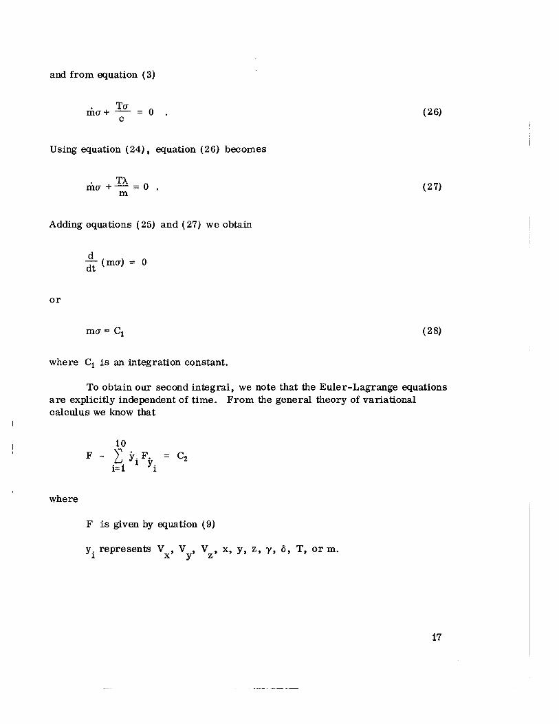
l and from equation (3)
m u + = C = 0 ,
I
I Using equation ( 2 4 ) , equation (26) becomes
m u + y = o . TA
Adding equations (25) and (27) w e obtain
d ma) = 0
o r
m u = Ci
where C, is an integration constant.
To obtain our second integral, we note that the Euler-Lagrange equations are explicitly independent of time. From the general theory of variational calculus we know that
10
i= 1 F - 9. F. = C,
1 Yi
where
F is given by equation (9)
y. represents V V , Vz, x, y, z, y, 6, T, orm. 1 x’ Y
17
Furthermore, since F is identically equal to zero, the above equation becomes
10 -c y . F. = C2 i= I 1 Y i
By differentiating and summation we obtain
Ai" + AzV + A,* Z + Vik + v2i + v3i 4- 0r;l = - c2 . Y
which may be written as
+ Taking the dot product of with *e as given by equation ( 2 1) and inserting
the result into equation (29) we find
The term in parentheses of this equation may be written
= irm + um
d dt
-- - (ma) = O ,
18
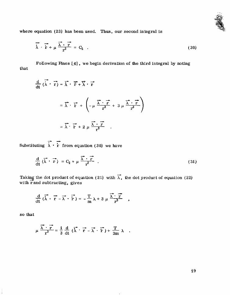
where equation (23) has been used. Thus, our second integral is
Following Pines [,6] , w e begin derivation of the third integral by noting that
4 4
Substituting > from equation (30) we have
Takins the dot product of equation (21) with r, the dot product of equation (22) with rand subtracting, gives
so that
- - A - r I d r , - - + - - T
1 - 1 7 = - - 3 dt 3m ( A ' r - h . j r ) + - - - ~ .
19
4 +
from this expression into equation ( 3 1 ) gives A - r 1.3 Inserting p
o r
d - 4 T - ( 2 ~ r + A * T>= 3 c 2 + - A . dt m
Now, using the defining equation be written as
d ? - - - - p - - ( 2 h r + A - r ) = 3C2 dt
for T in terms of m, equation ( 3 ) , this may
m - c A m .
To perform the integration we must f i rs t note that equations ( 2 4 ) and ( 2 8 ) yield
( 3 3 ) h = % C
making A a constant. Equation ( 3 2 ) now integrates to yield
- 4 - 4 mO
m 2 h r + A I. = 3C2t + C i I n -+ C 3 . ( 3 4 )
To obtain our final integral, we return to equations ( 2 1 ) and ( 2 2 ) . From these
4 - + - h x r h x r + p ~ = 0 r
20
Subtracting gives an immediately integrable equation yielding
- . - - - P r ) - z
h x r - h x r = C4
4
where C4 = (C4, C,, c6) is a vector integration constant.
To determine if the constants C4, C5, and (26 a r e independent, we apply the Jacobi test. Thus
c4 = jl2z - i3y - h2i + A&
c5 = i3x - i i Z - A3k + A i i
c, = i1y - i2x - hly + A2k . Now
ac ---fi=O ac ac ac ac ac ax a Y * az ax a Y - = i 3 , -=-ii , - - ; -5=-h3, -"=o , a ; = h l
ac ac a c , = o az Y $=A2 ' aj,
-=-i2, ac -Lii ac , ax a Y az
we may write
21
A non-vanishing sub-determinant is
0 z -y
A = -Z 0 x
y -x 0
in general, so our integration constants C4, C5, and c6 a r e independent.
= ZXY - ZXY E 0
The preceding statement cannot be taken to imply that w e may solve for - - -Dy 4
hi, &, and A3 in te rms of A , r , r , and Cd. To see this we write equation (35) as
Now
T so that w e cannot invert the coefficient matrix of (iI, jlz, i3) . his situation occurs in similar fashion with the angular momentum integral of the three-body problem.
DETERMINATION OF THE IAGRANGE MULTI PLIERS
The purpose of this section is to demonstrate three independent equations The f i r s t such which involve Lagrange multipliers &, A2, and A3 algebraically.
equation, equation (331, has already been derived. from equation (35). From this relationship we obtain
The second will be derived
22
4 t - D
since r ' ( A x r ) = O . To obtain our third relationship we first note that from equation (35) we
obtain
4
t - 7 r x (i, x 3 = F x ( E 4 + A x r ) , or
t - Inserting r - i from equation (30) into this expression gives
Now taking the cross product of ;with equation (35) gives
4 -
Introducing r A from equation (34) gives
m ( r . r ) h = -
2
7 Eliminating h between equation (37) and (38) under the assumption that
r - i- 20 gives - 4
23
t ?
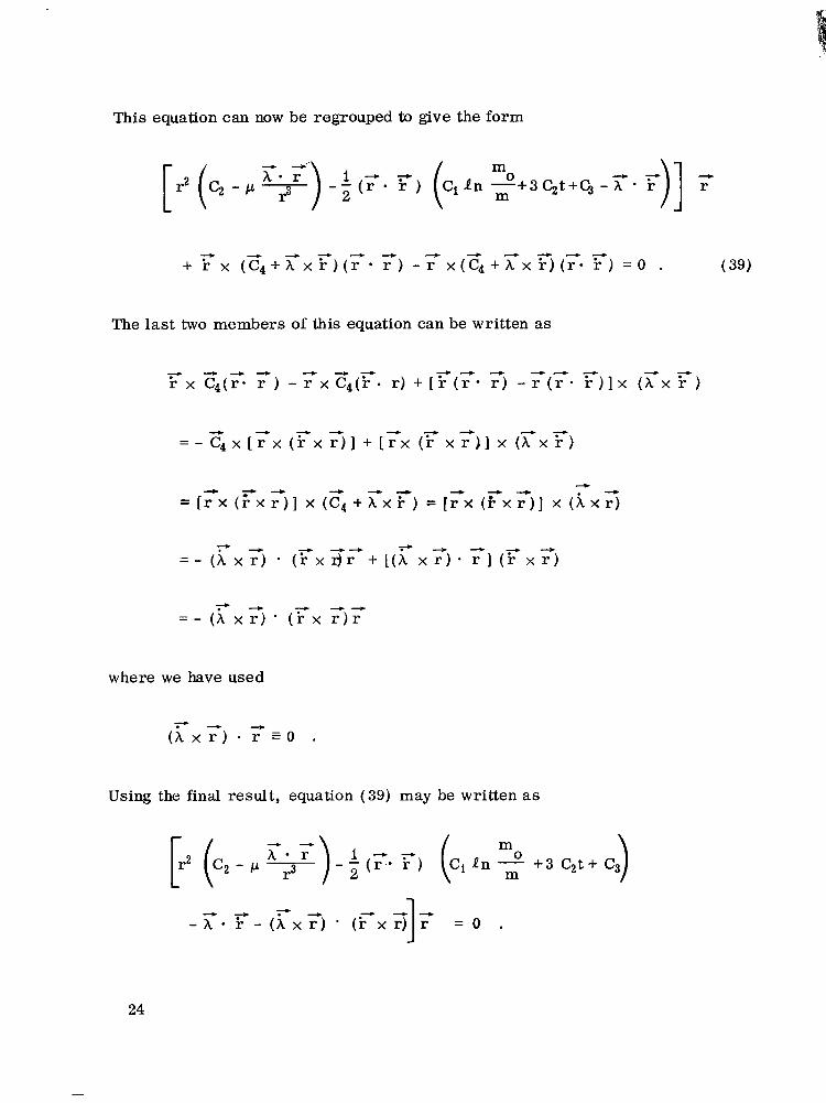
This equation can now be regrouped to give the form
The las t two members of this equation can be written as
* - D -- 4
= - (A x r ) * ( E x r ) r
where we have used
Using the final result, equation (39) may be written a s
24
- - - r
Since T'Z 0, the coefficient must vanish. Introducing A x r back into the coefficient yields
Equations (33) , (36), and (40) now define the Lagrange multipliers
Ai, A2, and A3 in te rms of r , r , m, and the integration constants. multiplier (T comes from equation (28) and vl, v2, v3 can be obtained from
equations (11) , (12), and (13) once A is computed from equation (35).
- 9 The
7-
DERIVATION OF THE M A S S FLOW RATE EQUATION
The preceding information is not sufficient for a complete solution of the problem for we do not yet know either m or T as a function of the problem variables. The necessary information is available, though obscure.
From equation (24),, which is the requirement that the singular a r c be followed, we have
ir i, A n i - - - + 2 = 0 . c m m
Inserting the values for iT and m we find that
i = O
or A is a constant which
L
5;'. 5;'- (?)' w e have ascertained from equation (33) . Furthermore
9
25
so that
and
From equation (22) w e obtain
The derivative of equation (42) is
but from equations (41) and (22)
26
so that equation (43) may be written
4 + * - 5 ( T - r ) ’ ( r - r ) = o .
By use of equation (34) , the previous equation may be written
The derivative of equation (44) is
27
Now c Z 0 for a powered arc , and assuming
we can solve for m, with m given by equation (44) , if
From equation (42), as noted by Corben [7] , w e may wri te
Since the left side of this equation is non-negative, we can w r i t e the angle be-
tween h and as a and conclude - I - 3 cos2 a 2 0
o r
I 3 - 2 C 0 S 2 Q .
Our criterion of equation (46) becomes
c o s 2 a f 3/5 .
Since this condition is excluded by the previous inequality, w e need only insure that
to s'olve for m; m is given by equation (44) .
28
CONCLUSIONS
The general problem of an optimal rocket trajectory in vacuo in an inverse square gravitationai field is composed of three possible types of seg- ments. The first of these is the coasting arc, and, for this case, a complete determination of the Lagrange multipliers as algebraic functions of the state variables, time, and integration constants has been obtained [ 1, 21.
The second case, sub-arcs of constant thrust, is most important from the practical standpoint and has not, as yet, yielded an analytical solution.
The third case is sub-arcs of optimal intermediate thrust (singular sub-arcs) and this area has been treated in this report. It has been shown that integrals which exist in the literature, equations (28) , ( 30), (34 ) , and (35 ) , are sufficient to explicitly yield the set of Lagrange multipliers which govern the guidance law along an optimal trajectory. The simultaneous algebraic equations governing the Lagrange multipliers associated with dynamical constraints are equations ( 33) , (36) , and ( 4 0 ) . Once this set of equations has been solved, equations ( 11) , ( 12), ( 13) , and ( 28) then yield the additional multipliers which were associated with kinematical constraints in the original formulation. Equa- tions ( 16) and ( 17) relate the Lagrange multipliers to the thrust direction angles. Finally, equation (45 ) supplies necessary information about the mass flow rate which is required to maintain the singular arc condition. Using these equations it is possible to compute an optfmal singular subarc without encountering the difficulties associated with the usual split boundary value problem.
George C . Marshall Space Flight Center National Aeronautics and Space Administration
Huntsville, Alabama, February 20 , 1967 933-50- 0 1- 00-62
29
h
5
RE FE RE N CE S
i. Eckenwiler, M. W. : . Closed Form Lagrangian Multipliers for Coast Periods of Optimum Trajectories. AIAA Journal, Vol. 3, 1965, pp. 1145-1 151.
2. Ng, C. H. and Palmadesso, P. J. : Analytical Solutions of Euler- Lagrange Equations for Optimum Coast Trajectories. The Boeing Co. , Huntsville, Alabama, NASA Accession Number N 66 34933.
3. Robbins, H. M. : Optimal Rocket Trajectories with Subarcs of Inter- 17th International Astronautical Congress ( Madrid, mediate Thrust.
Spain), Oct. 1966.
4. Kopp, R. E. and Moyer, A. G. : Necessary Conditions for Singular Extremals. AIAA Journal, Vol. 3, 1965, pp. 1439-1444.
5. Johnson, C. D. : Singular Solutions in Problems of Optimal Control. Volume I1 of Advances in Control Systems, Ch. 4, C. Leondes, ed. , Academic Press , 1965.
6. Pines, Samuel: Constants of the Motion for Optimum Thrust Trajectories in a Central Force Field. AIAA Journal, Vol. 2, No. 11, Nov. 1964; pp. 2010-2014.
7. Corben, Herbert C. : A Note on Optimization of Powered Trajectories in an Arbitrary Gravitational Field. Ramo-Woolridge, RW Rpt. ERL-IM-150, 4, Dec. 1957.
BIBLIOGRAPHY
I. Burns, Rowland E. : An Analytical Reduction of the Optimal Trajectory Problem. M. A. Thesis , University of Alabama, University, Alabama, August 1965. This thesis contains essentially the same material as is contained in this report.
2. Lawden, Derek F. : Optimal Trajectories for Space Navigation. Butterworth ( London) , 1963.