NASAContractor eport38 1 jNASA-CR-3851 19850007886
Fundamentals of Microcrack
Nucleation Mechanics
L. S. Fu, Y. C. Sheu, C. M. Co,
W. F. Zhong, and H. D. Shen
GRANT NAG3-340
JANUARY 1985
N//X
https://ntrs.nasa.gov/search.jsp?R=19850007886 2018-06-18T05:51:46+00:00Z
NASA Contractor Report 3851
Fundamentals of Microcrack
Nucleation Mechanics
L. S. Fu, Y. C. Sheu, C. M. Co,
W. F. Zhong, and H. D. Shen
The Ohio State University
Columbus, Ohio
Prepared forLewis Research Centerunder Grant NAG3-340
National Aeronauticsand Space Administration
Scientific and TechnicalInformation Branch
1985
TABLEOF CONTENTS
Page
SECTION
I. INTRODUCTION........................ i
II. TECHNICALBACKGROUND.................... 3
i. Definition of Microcrack Nucleation ........... 32. Microcracking in Polycrystals ............. 33. Microcracking in Ceramics and High Temperature Materials. 44. Dynamic Models of Microcracking ............. 45. Plan of Study ...................... 5
III. THEORETICALSTUDIES..................... 7
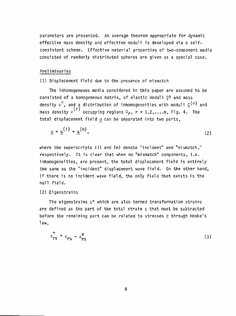
I, Preliminaries ...................... 8(i) Displacement field due to the presence of mismatch . 8(2) Eigenstrains .................... 8(3) Volume average and time average .......... i0(4) Volume integrals of an ellipsoid associated
with inhomogeneous Helmholtz equation ....... i0
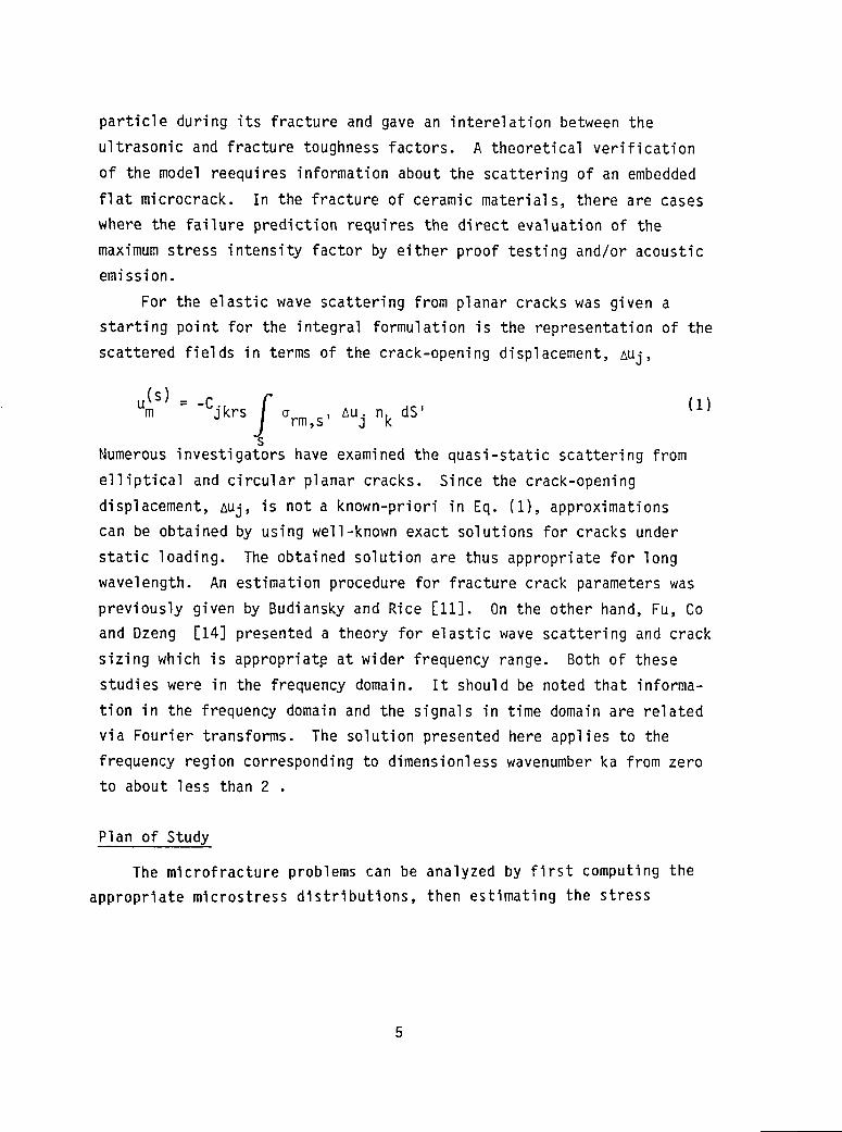
2. An Isolated Flat Ellipsoidal Crack ........... 12(i) Formulation and limiting concept .......... 12(2) Far-feild scattered quantities ........... 13(3) Determination of A_ and B_k .......... 15(4) Stress intensity factors and crack opening
displacement .................... 19(5) Numerical calculations and graphical displays 20
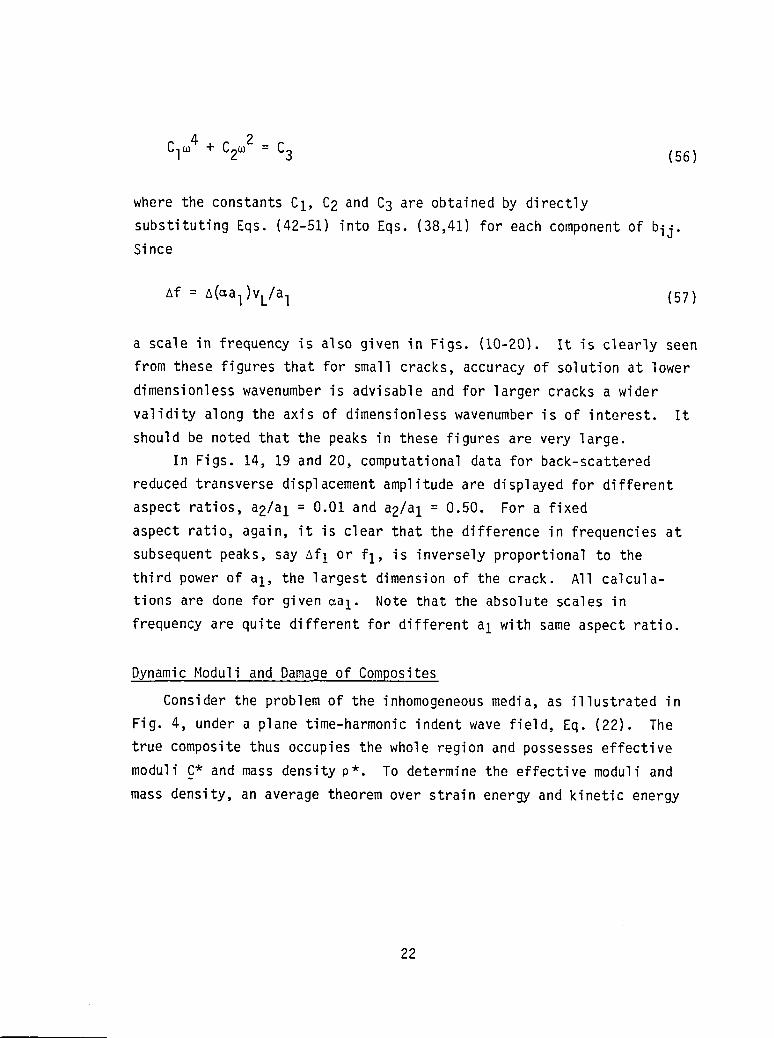
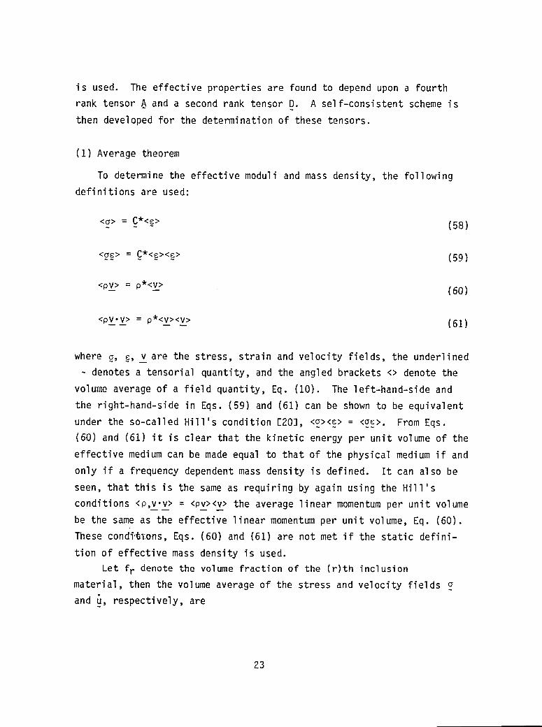
3. Dynamic Moduli and Damageof Composites ......... 22(i) The average theorem ................ 23(2) A self-consistent scheme for the
determination of effective properties ....... 26(3) Effective properties of two-component
media: randomly distributed spheres ........ 26(4) Example ...................... 28
IV. CLOSINGREMARKS....................... 31
REFERENCES............................ 34
APPENDIXA Volume Integrals Associated with the InhomogeneousHelmholtz Equation .................. 75
APPENDIXB The l-lntegrals and r-Functions ........... 78
iii
SECTIONI
Introduction
Previous theoretical [1-3] and experimental studies [4] established
the foundation for a correlation between the plane strain fracture
toughness klc and the ultrasonic factors ULB_/mthrough the
interaction of waves with material microstructures, i.e. grain size or
second-phase particle spacing depending upon the material system. This
• suggests a means for ultrasonic evaluation of plane strain fracture
toughness. Ultrasonic methods can therefore be used not only in the
evaluation of material properties such as moduli and porosity but also
in the fracture properties such as crack size and fracture toughness.
There are situations where material properties keep changing.
Stress induced deformation during manufacturing processes often cause
continued changes in material properties. It is well-known that pre-
cipitation, martensitic transformation, void nucleation, etc. often lead
to changes in material properties. Fracture toughness enhancement has
been observed in a number of ceramic systems due to stress induced
transformations e.g. Zirconia (ZrOz) particles contained in ceramic
matrix are observed to transform from a tetragonal to a monoclinic
crystal structure at sufficiently high stress environment. Circumferen-
tial microcracking may occur and a process zone is usually formed in the
vicinity of the stress raiser to reduce crack-tip stress intensity.
Precipitates, martensites and dislocations are typical examples of
inhomogeneous inclusions [5,6,27,32], i.e., regions with distributedtransformation strains alias eigenstrains. Since the scattered
displacements are directly related to the eigenstrains [7,8], thescattered field measured can be used to studied the changes caused by
the presence of precipitates, martensites, voids, etc.
The purposeof this work is to lay a foundationfor the ultrasonic
evaluationof mlcrocracklng. The work establishesan "average"theorem
and wave scatteringeffectsof a mlcrocrackand dlsbondedmlcrovold.
SECTION II
Technical Background
Definition of Microcrack Nucleation
A microcrack represents solid-vapor surfaces in a material and it
has a dimensional scale comparable to some microstructural features,
e.g. the grain size, The use of the term microcrack should not be con-
strued to imply brittle fracture. An microcracking event is obviously
the origin of fracture. In what follows, a brief review of different
mechanisms of microcracking is outlined.
Microcracking in Polycrystals
In single phase crystals, a microcrack nucleated from defect loca-
tions can grow at the competition between dislocation generation and
bond rupture of the crack tip. The activation or generation of disloca-
tions that pile up at the crack tip essentially determines whether the
crystal is brittle or ductile.
For cleavage-prone polycrystalline materials with brittle parti-
cles, such as A533B steel, the brittle fracture proceeds by a mechanism
involving a slip band blocked by a carbide. The most heavily strained
carbide particles are usually found to be a few grains ahead of the
crack-tip. The microcracking event therefore occurs at that location
under suitable loading conditions. For a polycrystalline material with
a matrix that resists cleavage the microcracking can occur by void
nucleation and growth mechanism. Stresses arising due to the incompati-
bility between the inhomogeneities and the material matrix may cause
eventual cracking of the particle (inhomogeneity) or the interface.
Depending upon the "size" of the particles involved, secondary
plastic zone near the inhomogeneities may or may not be of importance.
In essence, the continuum plasticity models can be used for large
3
inhomogeneities, _ _ 1 _mdetail dislocation structures must be
considered for the medium size particles, 0.01 _m _ 6 _ l_mand at the
decohesion of interface, the size of the plastic zone seems to be de-
pendent on the diameter of particles rather than the strains. Shearing
of the weak inhomogeneities may be an important mode of microcracking in
the case of very small particles, 6 _0.01 _m. It is clear from the
discussion above that the microcrack nucleation mechanism involves the
situations of either (1) the creation of new surfaces by tension or by
shear at a weak second-phase particle or (2} the nucleation and growth
of voids at a strong second-phase particle.
Microcracking in Ceramics and High Temperature Materials
The microcrack nucleation is an event of crack initiation. The
presence of a single microcrack is usually not of serious consequences.
It may, however, grow in size to become a macrocrack. Multiple
microcracks may nucleate near the vicinity of a macrocrack to form a
microfracture process zone thus enhance the coalescence of microcrack
that add to the length of a macrocrack. Voids nucleated along grain
boundaries may be flatened out into cracks under favorable conditions.
Spacing between the voids, can be strongly dependent both on distance
from the crack and on the duration of loading [32]. One form of
transformation toughening of ceramics with intercrystalline ZrO2 dis-persions was found to be largely caused by microcrack nucleation and
extension. The phenomenonof fracture toughness enhancement was ex-
plained by the use of circumferential microcracking model [30] and by a
continuum elastic plastic fracture mechanics approach.
Dynamic Models of Microcracking
A simple dynamic model for microcracking was first proposed by Vary
[4] where he considered the stress wave energy required to create a
microcrack of the diameter same as the second-phase particle. He
considered this potrion of the energy to be totally consumed by the
particle during its fracture and gave an interelation between the
ultrasonic and fracture toughness factors. A theoretical verification
of the model reequires information about the scattering of an embedded
flat microcrack. In the fracture of ceramic materials, there are cases
where the failure prediction requires the direct evaluation of the
maximumstress intensity factor by either proof testing and/or acoustic
emission.
For the elastic wave scattering from planar cracks was given a
starting point for the integral formulation is the representation of the
scattered fields in terms of the crack-opening displacement, Auj,
u_s) = -Cjkrs f Orm,s, _uj nk
(1)dS'
S
Numerous investigators have examined the quasi-static scattering from
elliptical and circular planar cracks. Since the crack-opening
displacement, Auj, is not a known-priori in Eq. (i), approximationscan be obtained by using well-known exact solutions for cracks under
static loading. The obtained solution are thus appropriate for long
wavelength. An estimation procedure for fracture crack parameters was
previously given by Budiansky and Rice [11]. On the other hand, Fu, Co
and Dzeng [14] presented a theory for elastic wave scattering and crack
sizing which is appropriate at wider frequency range. Both of these
studies were in the frequency domain. It should be noted that informa-
tion in the frequency domain and the signals in time domain are related
via Fourier transforms. The solution presented here applies to the
frequency region corresponding to dimensionless wavenumber ka from zeroto about less than 2 .
Plan of Study
The mlcrofracture problems can be analyzed by first computing the
appropriate mlcrostress distributions, then estimating the stress
5
intensity factor K for typical microstructural defects located in the
stress field, and finally equating K to the local material resistance to
microfracture. The microfracture problem of greatest practical interest
concerns the grain shape, size, and relative orientation that dictates the
onset condition for boundary mlcrofracture between grains.
As a beginning in this program, the elastic wave scattering from a
planar crack under incident plane waves is studied. The specific
geometries studied are the penny-shaped circular crack and the elliptical
crack. Far-fleld quantities such as the reduced scattering amplitude that
are related to the shape, size and orientation of the crack will be
determined. Near field quantities such as the crack size, the stress
intensity factors and the crack opening displacements are briefly studied
[13,14]. The approach taken is based upon the methods developed in
[7,8,12].
As a second part of the work for this program, an average theorem is
developed to study the dynamic effective properties of media with randomly
distributed Inhomogeneltles. The approach taken is deterministic in
nature and the solution is based upon the elastic wave scattering of a
single Inhomogenelty, a self-conslstency scheme and an averaging theorem
over strain energy and kinetic energy [8,15].
6
SECTIONIII
Theoretical Studies
The aim in non-destructive evaluation (NDE) by sound and ultrasound
is to extract material and fracture properties from pulses sent and re-
ceived at transducers. The analysis is usually given either in the time
domain or the frequency domain. The introduction of the size factor,
the wavelength, in the model mechanics problems in NDE, plays the impor-
tant role of relating the far-field measurable quantities such as phase
velocities and attenuation to the near-field physical situation such as
local geometric dimensions and elastic properties. This aspect of the
analysis thus allows "nondestructive" testing methods to be employed for
"experimental" validation of the predictions by the theories.
Solution to the elastic wave scattering due to a single embedded
inhomogeneity is available by different methods that are appropriate at
different frequency ranges [16,10]. The methods that offer a solution
in an analytic form and are useful for inhomogeneous media with multiple
components are the longwave approximation, the polarization approach and
the extended method of equivalent inclusion [7,8].
There are several averaging schemes or theorems that exist in the
literature for finding the dynamic effective moduli and mass density.
While some efforts concentrate on the average stress _ and strain
fields or on the average displacement field u, others concentrate on a
variational approach. These theories are appropriate mostly at Rayleigh
or longwave limits and do not exhibit dispersive effects. Dispersive-
ness and attenuation are important in dynamic material propertiesevaluation.
In what follows, the scatter of elastic waves due to a thin flat
ellipsoidal inhomogeneity is first studied. Penny-shaped and ellipti-
cally-shaped cracks are studied as special cases. Fracture crack
parameters are presented. An average theorem appropriate for dynamic
effective mass density and effective moduli is developed via a self-
consistent scheme. Effective material properties of two-component media
consisted of randomly distributed spheres are given as a special case.
Preliminaries
(1) Displacement field due to the presence of mismatch
The inhomogeneous media considered in this paper are assumed to be
consisted of a homogeneousmatrix, of elastic moduli COand masso
density p , and a distribution of inhomogeneities with moduli C(r) and(r)
mass density p occupying regions _r, r = 1,2, .... n, Fig. 4. The
total displacement field u can be separated into two parts,
: _(i) + _(m), (2)
where the superscripts (i) and (m) denote "incident" and "mismatch,"
respectively. It is clear that when no "mismatch" components, i.e.
inhomogeneities, are present, the total displacement field is entirely
the same as the "incident" displacement wave field. On the other hand,
if there is no incident wave field, the only field that exists is thenull field.
(2) Eigenstrains
The eigenstrains _* which are also termed transformation strains
are defined as the part of the total strain _ that must be subtracted
before the remaining part can be related to stresses _ through Hooke's
law,
e (3)_rs = _rs - _rs
8
e = C-I_rs jkrs °jk (4)
where C-I are the elastic compliances. The method of equivalent
inclusion is a method that allows the inhomogeneous media be replaced by
media of homogeneousmatrix effective moduli with distributed trans-
formation strains in the regions originally occupied by inhomogeneities,
hence
* I 0 in £o (5)Srs = I * in _r r : 1,2...n.Crs
For the two prolems to be equivalent, the transformation strains must
give rise to a field that is exactly the same as that of the "mismatch"
field, u(m). This leads to equivalence conditions that insure
identical field quantities at any given point be obtained in the two
probl erosf [9]:
u(m)(r)+Cj _I)(F) = -ACj u(i)(F) in _ (6)ACjkrs r,s krs krs r,s '
2 u!i)(F) in R (7)2 m)(r) + Cj *(2)(F)= -ApAp u krs _rs,k J
There are two types of transformation strains or eigenstrains that
arise in elastodynamic situations due to the mismatch in elastic moduli
Ac and mass density Ap. It is often convenient and useful to define
associated quantities such as
) (8)mjk = Cjkrs Sr
tThe conditions (6.7) are similar to those of Willis (1980) andthose of Mura, Proc. Int. Conf. on Mechanical Behavior of Materials, 5,Society of Materials Science, Japan, 12-18 (1972).
*(2)xj : Cjkrs _rs,k (9)
where mjk and _j are referred to as momentdensity tensor and
equivalent force or eigenforce, respectively.
(3) Volume average and time average
The volume average and time average of a field quantity say F(r,t)
is denoted by using brackets < >, and < >T, respectively, and aredefined as
<F(_,t)>: _ f F(_,t)dV (i0)
1<F(r't)>T: T : F(_r,t)dT (11)
where V and T stand for volume and time period, respectively.
(4) Volume integrals of an ellipsoid associated with inhomogeneousHelmholtz equation
Volume integrals of an ellipsoid associated with the integration of
the inhomogeneous Helmholtz equation are used in this work. The
inhomogeneous scalar Helmholtz equation takes the form:
V2_ + k2_ = -4_y(_) (12)
whereY(_) is the sourcedistributionor densityfunction,v2 and k are
the Laplacianand wavenumber,respectively. A particularsolutionto
Eq. (12) is
_(_) = $ Y(_')R-lexp(ikR)dV', R = Ir_-_'I (13)
I0
in which (4xR)-lexp(ikR) is the steady state scalar wave Green's
function and g is the region where the source is distributed. The
source distribution function Y(r) can be expanded in basis functions or
polynomial form, depending upon the geometry of volumetric region _.
For an ellipsoidal region, the choice of using a polynomial expansion
separates this work from other theories of elastic wave scattering:
Y(_') = (x')X(Y')P(z') v (14)
in which _, _, v are integers.
For elastic wave scattering in an is,tropic elastic matrix, two
types of volume integrals and their derivatives need to be evaluated:
_(_) : % R-lexp(i_R)dV ' (15a)
_k(r)_ : f X'k R-lexp(i_R)dV' (15b)
_Ukj_...s(r) : f x_x_...XsR-lexp(i_R)dV ' (15c)
oao
_,p(r) - _- aXp _(_) (16a)
_pk,p(r) _ _k(r) (16b)
oo.
2 2/V _ 2/where _ = = pe (X + 2u). The other type, the O-integrals, are
obtained by replacing _ with 6 in Eqs. (13,14), where B2 = pm/(mu)
Details of the integration are given in [12]. In this work only
limiting value at r_O and r+ _ are of interest.
II
An Isolated Flat Ellipsoidal Crack
(1) Formulation [28,13,8]
Consider the physical problem of an isolated inhomogeneity embedded
in an infinite elastic solid which is subjected to a plane time-harmonic
incident wave field as depicted in Fig. I. Replacing the inhomogeneity
with the same material as that of the surrounding medium, with moduli
Cjkrs and mass density p, and include in this region a distribution of
eigenstrains and eigenforces, the physical problem is now replaced bythe equivalent inclusion problem.
The total field is now obtained as the superposition of the inci-
dent field and the field induced by the presence of the mis-matches in
moduli and in mass density written in terms of eigenstrains c*_ I) and
eigenforces, x_
F = F(i) + F(m)- ~ ~ (17)
where F denotes either the displacement field uj, the strain field
cij, or the stress field _ij. The superscripts (i) and (m) denote
"incident" and "mis-match", respectively.
For uniform distributions of eigenstrains and eigenforces, thefields can be obtained as:
um(m)(r') : - 7" ' Cj l)Sjm,k, (_ j Sjm(r)- r') (18)
(m)=, (m)+ u_mm))/2Cmn £Um,n (19)
(m) (m)_Pq = Cpqmn_mn (20)
12
where a commadenotes partial differentiation and
SJm(_) = f_ gJm(_-_')dV' (21)
in which gjm is the spatial part of the steady state elastic wave
Green's function and _ is the region occupied by the inhomogeneity. It
is noted that the integrals Sjm and their derivatives must be
evaluated for the region _ > _' and for the region r < r', Ref. 12.
The solution form represented in Eqs. (15-19) gives the fields inside
and outside an isolated inhomogeneity of arbitrary shape.
(2) Far-field scattered quantities
Let the incident displacement field be longitudinal and of
frequency m, amplitude uo:
u_i) : uoqj exp[i_xik i - i_t] (22)
where i 2 = -1 and qj is the unit vector in the normal direction of
the plane time harmonic wave and k i is wave vector. For a linear iso-
tropic medium, the spatial part of the free space Green's function is
well known. Substituting gjm(r-r') in Eqs. (19,21) and using thelimiting concept 13:
limit a3 x* = Aj constants (23)a3.O J
limit a3 €_ I) = Bij constants (24)a3.O
13
the scattered displacement u_ )f= (r,t) from a thin elliptical flat crack
can easily be obtained as:
(s) (r,t) um(m)(r,t)Um _
(_al)3Uo (_al)3Uo r . _ (25)
= [(C Gmexpi_r)/mr + (D HmexpiBr)/Br]exp(-i,.,t)
where
Gm = - (a2/al)[-_m_jA _ + (l-2m2/B2)_mB_j+2(_2/B2)_m_k_jB_j] (26)
Hm = (a2/al)[-(B/m)3(_m_j-6mj)A_
- 2(B/m)2_kB_m + 2(B/m)2_m_k_jB_j ]
C = [jo(_re)+J2(_re)]/3 : sinmre/(mre )3 - coS_re/(_re )2 (27)
D = [jo(Bre)+J2(Bre)]/3 = _nBre/(Bre )3 - coSBre/(Bre )2
2= a_r e
in which m,j,k = 1,2,3, and (al,a2), _m, m, B, denote the
semi-axes of the flat ellipsoidal crack, direction cosines of scattered
displacements, longitudinal wavenumber, shear wavenumber, respectively.
Also, Aj and Bjk are the reduced non-dimensional form of Aj and
Bjk, respectively, defined as follows:
/(&pm2Uo) &p = p' -p , (p' = 0 for a crack) (28)Ae AJ J
14
B _
jk : -Bjk/(i_Uo) (29)
Expressions for the differential cross section dP(m)/dQ and total
cross section P(m) can be obtained as [19]:
dP(_) = L(e,, ) + (_/B) T(e,@) (30)d_
P(m) = fs[_L(e,@)+ (_/B)_T(e,_)]d£ (31)
where d_ is the differential element of solid angle and
_2_t(e,_) = (_al)6[C gm][C---_]m (32)
B2_T(e,@): (_al)6[DHm][D---_m (33)
in which the super bars denote complex conjugate. It is noted that the
constants A_ and B_k must be evaluated from the equivalence
conditions Eqs. (6,7) with the use of the limiting concepts in Eqs.
(22,23) and of the integration method developed in Ref. [12].
(3) Determinationof A_ and B_k
In Eqs. (22-26)the scattereddisplacementfield is given in terms
of the "reduced"formof the eigneforcesand eigenstrains,i.e.A_and
B_k. These constantsmust in turn be determinedfrom the equivalence
conditions. Writingthe incidentwave field in a Taylorseriesthe gov-
erning simultaneousalgebraicequationscan be easilyobtained. Since
fij[O]and Fmij[O]vanishautomatically,these governingequations
becomeuncoupledand lead to a three by three systemfor A_ and a six,
by six systemfor Bjk. For a linearelasticmedium,they are:
15
Apm2Uofjs * =[O]A_ + As - qs (34)
{A_6stDmmjj [0] + 2A_Dstjk[O]}B_k + {_6st B*mm+ 2uB_t}
= _ {AX_stqmqm + 2A_qsqt} (35)
where the subscripts s,t,m,j,k = 1,2,3 repeated subscripts denote sum
from I to 3, and
4_o 2fjs(_) = _ _2¢ _js + _'mj - ¢'mj (36)
4xpm2 Dstjk(Z)= 2u[@,stjk+ ¢,stjk]
- uB2[¢,jt_ks+ ¢,js6kt] (37)
_ _2 @,mnajk
in which
AX = -X, Ap = -p, Ap = -p
The €- and @-integrals and their d_rivatives are evaluated by the
method suggested in Ref. [12]. Retaining terms up to (_aI) or (BaI)of the fourth order, the constants are obtained as:
qj/{Uo_2Apfj[O]+ I} no sum on j (38)A_j
i
fj[O] = (fll[O], f22[0], f33[0]) (39)
16
{B_} : [bij]-l[cj] i,j = 1,2,3 (40)
* qiqj/[l{B..} = - + _(_i[0] + {j[0])], no sum on i,j.13i # j (41)
i,j = 1,2,3 _ = I/4_
where in Eq. (37) B_ : B_I , B_ : B_2 , B_ : B_3 ,
cj = (Ax + 2Ap)[l + q_] , j = 1,2,3, (42a)
bll = (x + 2_) + xc_,jj[0] + 2(x + 2_)_@,ii[0] + 2_C_,iI[0] (42b)
b12 : x + x_@,jj[0] + 2_@,ii[0]+ 2_x_,22[0] (42c)
b13 = _ + _@,jj[0] + 2_@,ii[0] + 2_,33[0] (42d)
b21 = _ + _@,jj[0] + 2_@,22[0] + 2_,ii[0] (42e)
b22 = (_ + 2_) + _c@,jj[0] + 2_@,22[0] + 2_(_ + 2_)@,22[0] (42f)
b23 = _ + _@,jj[0] + 2u_@,22[0] + 2_@,33[0] (42g)
b31 : _ + _@,jj[0] + 2_,33[0] + 2_,Ii[0] (42h)
17
b32 = _ + _,jj[O] + 2_,33[0] + 2_,22[0 ] (42i)
b33 = (_ + 2_) + _@,jj[O] + 2u_@,33[0]+ 2(_ 2u)_,33[0] (42j)
.[0]Note that bij _ bji. In Eq. (38), _I = @II " _2 = _22[0]' _3 : _33[0]"
The f- , _- functions are given as:
4xpm2 fjs[O]= - B2@[O]6js+ @,js[O]- @,js[O] (43)
B2@[O]= xala2B2{lo - ((Bal)2/16)ll + i(8/3)B} (44)
@,ii[0] = -[(xa_a2B4)/12)]. I l (45)
@,22[0]= -[(xala_B4)/12]. I 1 (46)
@,33[0] = 0 (47)
in which
I : f = F(e,k).al (48)o o
ii : %_ _d_ _ 2 {E(e,k) k '2o (a_ + _)A(_) al k2 - kT F(e,k)} (49)
18
12 = f_ _d@ _ 2 {F(o,k) E(e,k)2 al k2 k2 } (50)o (a2 + @)A(@)
F = I e dm E = fe (l_k2sin2)I/2dm (51)o (l_k2sin2m)I/2 ' o
and as a3.O, o_/2, k2.(l 2 2 k,2 .2, 2. 2-a2/al) and = (I-K).a2/a I, if aI > a2. If
a3.O and aI = a2, we have Io = _/al' II = 12 = _/2al" The 4@- functionsare obtained by replacing B with _ in the € - functions.
(4) Stress Intensity Factor (SIF) and Crack Opening Displacement (COD) -preliminary results.
The general expression for the total displacement field can be
easily obtained, by using Eq. (2) and the expression for the mis-match
displacement field [9], as follows:
Um(_) = fmJ(_)AJ + fmjk(_)Ajk+ (52)
+ Fmij(_)Bij + Fmijk(_)Bijk. ....
To find the crack face opening displacement the functions f< and F<
must be evaluated for r inside the crack.
In this section, the solution for a crack is that degenerated from
an ellipsoidal void by letting a3+O. The crack opening displacement
for an elliptical crack can be defined as
AUi = 2Ui : h(_ i + x#) (53)
where h is the half thickness of the ellipsoidal void in the
x3-direction:
19
h = a3(1 2 2 2- 2,1/2- xl/al- x2/a2_ (54)
For the case of uniformlydiistributedeigenstrainsand eigenforces,
the crack openingdisplacementis, therefore,obtainedas:
z_uj= [(Ai + B3j)a3h]a3+0
]• 1Uo a_ a-_JL--pA* B_i
where uo is the amplitudeof the incidentwave field and Aj and
B3j are given by Eqs. (38-41).
The stress intensityfactorscan be easilyobtainedby findingthe
strain energychange W, i.e.the interactionenergy,due to the
presenceof the crack and then differentiatewith respectto the crack
dimension. An approximationfor low frequencyrange can be obtainedby
using the SIF-CODrelation[11]. Surface-waveinteractionwith an edgecrack was studiedin [33].
(5) Numericalcalculationsand graphicaldisplays
It is clear from Eqs. (38-41)that the uniformlydistributedeigen-
strainsand eigenforces,in their reducedform, Bij and Aj, respect-ively,are dependentonly upon the incidentwave field characteristics
and the geometricfactorsof the inhomogeneityfor a given material
system. It is observedfrom Eqs. (38-42)that Bi and Bij as
functionsof dimensionlesswavenumberof aI or aI would exhibit
large peak values at certainincidentwave frequencieswhen bij O.
The valuesof these criticalfrequenciesdependonly upon the matrix
elasticmoduli,the crack dimensionsand the measurementdirection. For
a given crack aspectratio,a2/al,and a measurementdirection,
the differencein frequenciesat subsequentpeak valuesis proportional
to aI, the largestdimensionof the crack, Fig. 9.
20
Computational data of elastic wave scattering due to a flat crack
embeddedin any given isotropic material system can be obtained by
employing Eqs. (25-29) and (34-51) with Ap = -p, A_ = -_ and A_ = -u.
Scattered displacement amplitudes can easily be obtained for any given
crack aspect ratio.
(a) Elliptical Crack: In Figs. 7-9 computational data for back
scattered situation are displayed for a crack in aluminum of different
crack aspect ratios, i.e. a2/a I = i, 1/2, i/i0 at various wave
incident angle. Critical frequencies are observed to be present in
Bij but no critical frequencies are identified for Aj, j = 1,2,3
Figs. 10-13. The critical frequencies for CIGml and D[Hm[ are,
however, clearly identified. The position along the _aI axis at which
the first critical frequency occurs depend upon the crack aspect ratio
and matrix elastic moduli. Sufficiently small increment in _aI must
be used in order not to miss any peak values. Since the soulution form
given in Eqs. (25-27,38-51) is analytic in frequency, this can easily be
achieved. It is noted that most of the scattered energy is carried by
the transverse components of the scattered displacement, i.e.
IDHml > ICGml, Figs. 14,15.
(b) Penny-shaped Crack: In Fig. (7), the reduced longitudinal back
scattered displacements at _ = ¢ = 45o and the samecrack aspect
ratio, a2/a I = 1, are shown for a crack in structural steel. The
change in the absolute value of the crack size causes a compaction of
the peaks in ICGml along the axis of dimensionless wavenumber _aI.
It is of interest to observe that the difference in frequencies at
subsequent peak values, e.g. the first and the second peaks, Af I, is
inversely proportional to a certain power of a1. This fact can easily
be algebraically demonstrated by using Eq. (42) to find the critical
frequencies, i.e. finding the roots of the following algebraic equation:
21
Clm4 + C2m2 = C3 (56)
where the constants C1, C2 and C3 are obtained by directly
substituting Eqs. (42-51) into Eqs. (38,41) for each component of bij.Since
Af = A(mal)vL/a I (57)
a scale in frequency is also given in Figs. (10-20). It is clearly seen
from these figures that for small cracks, accuracy of solution at lower
dimensionless wavenumber is advisable and for larger cracks a wider
validity along the axis of dimensionless wavenumber is of interest. It
should be noted that the peaks in these figures are very large.
In Figs. 14, 19 and 20, computational data for back-scattered
reduced transverse displacement amplitude are displayed for different
aspect ratios, a2/a I = 0.01 and a2/a I = 0.50. For a fixed
aspect ratio, again, it is clear that the difference in frequencies at
subsequent peaks, say Af I or fl, is inversely proportional to the
third power of al, the largest dimension of the crack. All calcula-
tions are done for given ma1. Note that the absolute scales in
frequency are quite different for different aI with same aspect ratio.
Dynamic Moduli and Damageof Composites
Consider the problem of the inhomogeneous media, as illustrated in
Fig. 4, under a plane time-harmonic indent wave field, Eq. (22). The
true composite thus occupies the whole region and possesses effective
moduli C* and mass density p*. To determine the effective moduli and
mass density, an average theorem over strain energy and kinetic energy
22
is used. The effective properties are found to depend upon a fourth
rank tensor A and a second rank tensor D. A self-consistent scheme is
then developed for the determination of these tensors.
(1) Average theorem
To determine the effective moduli and mass density, the followingdefinitions are used:
<_> = C*<_>_. (58)
<g_>= C*<_><_> (59)
<pv_>= p*<v_> (60)
<pv-v>: p*<v><v> (61)
where 9, _, v are the stress, strain and velocity fields, the underlined
~ denotes a tensorial quantity, and the angled brackets <> denote the
volume average of a field quantity, Eq. (i0). The left-hand-side and
the right-hand-side in Eqs. (59) and (61) can be shown to be equivalent
under the so-called Hill's condition [20], <_><_> = <_>. From Eqs.
(60) and (61) it is clear that the kinetic energy per unit volume of the
effective medium can be made equal to that of the physical medium if and
only if a frequency dependent mass density is defined. It can also be
seen, that this is the same as requiring by again using the Hill's
conditions <p,v-v> : <pv><v> the average linear momentumper unit volume
be the same as the effective linear momentumper unit volume, Eq. (60).
These condi._1_ons,Eqs. (60) and (61) are not met if the staticdefini-
tion of effectivemass densityis used.
Let fr denote the volume fractionof the (r)th inclusion
material,then the volumeaverageof the stressand velocityfields
and u, respectively,are
23
n
<_> : _ fr_(r) (62)r--o
n
<u_>= z fr_(r) (63)r=o
where (r) = G(r)_(r), (r) = 0,1,2,....n,
and for time-harmonic situation
= v = -imu (64)
Equations(59)and (61)can be rearranged,by using Eqs. (62)and
(63), as
n (r)_(<_> = C°<_><_> + Z fr C r)<_> (65)r=l - ~ "
n (r)v(r)<v><pv,v> : p°<v><v> + z f Ap (66)r=l r - -
Considernow the case when the solutionform possessesa linear relation
betweenthe velocityand strainfieldsin the (r)thcomponentand the
averagevelocityand strainfieldsof the effectivemedium, i.e.
_(r) = A(r)<_> (67)
_(r) : D(r)<v_> (68)
24
where A(r) and D(r) are tensors of fourth and second rank that must
be determined with a suitable scheme. The substitution of Eqs. (67) and
(68) in Eqs. (65) and (66) leads to
n fraC(r)A(r )<q_> = {cO + _ ~ ~ }<_><_> (69)r=l ~ ~
n frAp(r)D(r)<pvv___>= {po + z }<v><v> (70)r=l ~
A comparison of the above with Eqs. (59) and (61), the expressions for
the dynamic effective moduli and mass density are obtained as follows:
n frAC(r)A(r )C* = C° + z (71)r:l
n (r)D(r) D(r) _)p. = pO + z frAp = D /3 (72)r:l
It is important to note that the tensors A(r) and D(r) are frequency
dependent and they replace the static expressions when frequency
approaches zero and when proper cares are taken. The assumption of a
general linear dependence between _(r) and <v_>,Eq. (68), will have to
be specialized such that the second rank tensor D will degenerate into a
scalar. This specialization is automatic for randomly distributed
spheres where Dmj = D_mj, in which D = DII = D22 = D33.To determine the explict form of the tensors A(r) and D(r), the
strain and velocity fields in the (r)th component are determined by
using the method of equivalent inclusion as presented in the previous
section.
25
(2) A self consistent scheme for the determination of the effectiveproperties
The tensor fields A(r) and D(r) are of ranks four and two, re-
spectively, and they are functions of wavenumbers, geometric properties,
and effective and inclusion material properties. Let the average strain
and velocity be the same as those derived from the incident wave field,
then the governing conditions for determining A{r) and D(r) for the
(r)th inclusion are simply obtained by rewriting the equivalence condi-
tions for an effective medium with mass density p* and moduli C*:
c(r)(_(i)+_(m)) : C.(_(i)+_(m)__.)_ , in _r (73)
p(r),.2(y(i)+y(m)) : p. 2(y(i)+y(m)) _ #, in _r (74)
where the superscripts (i) and (m) stand for "incident" and "mis-match",
respectively, Slightly different approaches for finding effective
moduli for hetrogeneous material are given in [20,23] that apply to
static cases with different constituents and situations. The strength
and fracture responses of composites have been investigated [17,18,20-23].
(3) Effective properties of two-component media: randomly distributedspheres
Let the moduli, mass density for the matrix, inclusion material0
particles and the effective medium by denoted by Cjkrs , pO; Cjkrs,p'; and Cjkrs and p*, respectively. Using the elastodynamic solution
for a single ellipsoidal inhomogeneity, the displacement and strain
fields inside an inhomogeneity are found, when the average displacements
are made equal to the incident time-harmonic plane wave field, to be:
26
[u(m)(_)] = D(_)u(i) _ _(_)u(i), in _r (75)
[_(m)(_)] = A(r)_(i) _ _(_)u(i), in Rr (76)
in which the superscripts (m) and (i) denote "mis-match" and "incident",
respectively. Employing the volume averaging process as described by
Eq. (10) and substituting in Eqs. (65,66), the effective properties are
easily defined as follows:
p* = p + fApD, D = 13-Djj (77)
C* = C + fACA (78)
where f is volume fraction of inclusion material. The tensor fields
and A are:
Dmj = -<fmj(K)>/{fMj[O] + 4_o'-p*)m2}, no sum on M,J. (79)
Amnpq = <Fmjk,n(_ ) + Fnjk,m(_)>Sjkpq/2p*_ 2 (80)
in which the tensors f and F are defined as:
4_p_2fmj(_ ) =_2€6mj + _'mj - ¢'mj (81)
4_p_2Fmij(_) = -[_2@,m6ij + 2_B2¢,iamj - 2_@,mj + 2U¢,mj] (82)
The ¢- andS-integrals given in Eqs. (15,16), etc. are the volume
integrals associated with the inhomogeneous Helmholtz equation. They
can be carried out for an ellipsoidal region by expanding (exp ikR)/R in
27
Taylor series expansions with respect to r', for r > r' and with respect
to r for r < r'. Here k can be either _ or B. Details are given in
Ref. [12]. This type of expansion for the integrand is particularly
useful in determining the coefficients of a "polynomial" distribution of
* *} 1)_j and _i •
The fourthrank tensor Sjkpq is the connectingtensorbetweenthe
eigenstrainsand the appliedstrains,i.e.
_.(I) (a) : Sj C ai,_)jk = Sjkpq pq ' Sjkpq kpq( ' (83)
for the case of uniform eigenstrains and eigenforces. In developing
these expressions the volume average of the _-integrals, must be
evaluated. Finally, it should be noted that p* and C* are complex where
the real and imaginary parts are associated with the velocity and
attentuation, respectively.
(4) Example: spherical inclusion materials
Let the spherical inclusion materials of radius "a" be randomly
distributed over the whole volume of the matrix. If the matrix and the
inhomogeneities are isotropy, the effective medium is also isotropic.It is straight forward to show that
Dmj = _mj {-<f33(_)>/f33[O]+ 4_(p' - p.) 2] (84)
= _mjDand
Sjkpq = Skjpq = Sjkqp = Spqjk
Sll I : $2222 = $3333 = C1 (85)
S2323 = S1313 = S1212 : C3
Sl122 = Sl133 = $2233 = C2
28
where
C1 = (C_ + C_ - 2GC_)/[(C_) 2 + C_C_- 2(C_)2]
C2 = (C_G - C_)/[(C_) 2 + C_C_ - 2(C_) 2]
C3 = {2F122,1[0] + u*/(_' - _*)}
C_ = GFIII,I[O] + (G+I)FI22,1[O] + H
C_ = FIII,I[O] + 2GF122,1[0] - F
F _ -(_* + 2_*)/G
G = (_' - _*)I[(_' - _*) + 2(_' - u*)]
H = x/G
Following the theory developed in the previous sections, the
effective moduli and mass density are found to be
P* : P . fApD (86)
_* = _ + fIAt(All11 + 2AI122) + 2A_AII22] {87)
_* = u + fA_(AI212 + A1221) (88)
K* = K + f[(Allll + 2AII22)A_
+ (2/313AI122 + A1212 + AI221)A_] (89)
29
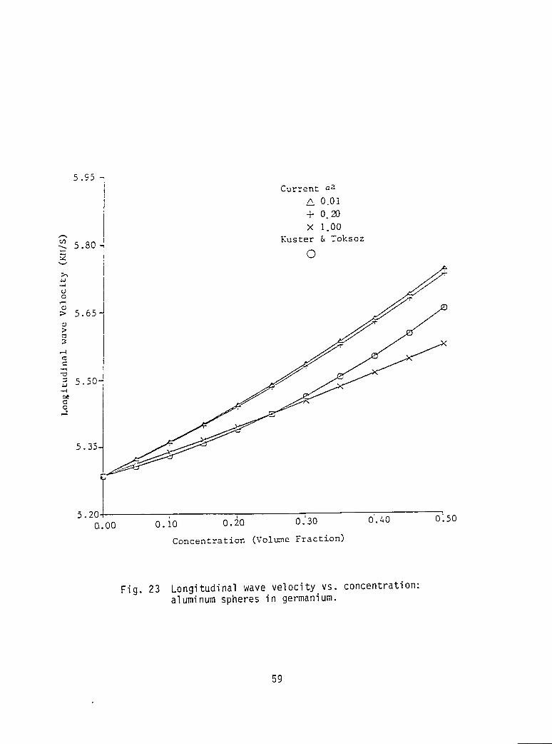
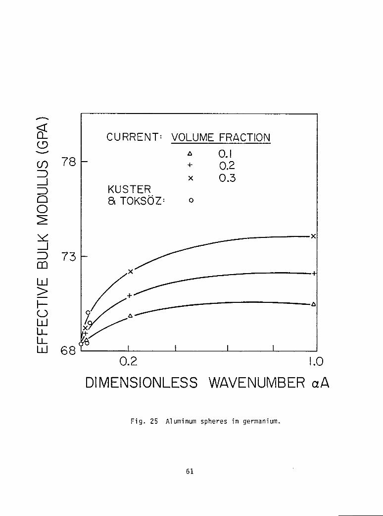
It is clearly seen that the velocities are dispersive. At frequency
range above that of the Rayleigh limit, this phenomenon is pronounced.
From Figs. 21-23, the bulk moduli, shear moduli and longitudinal veloci-
ties are shown as functions of volume concentration of spherical
inclusion materials for the cases of aluminum spheres in germanium, for
different dimensionless wavenumbers _a. For a given fixed concentra-
tion, the moduli K*, u* and velocity VL and VT are increased as the
dimensionless wavenumber_a is increased. The dispersiveness of effec-
tive shear modulus is minimal and that of effective bulk modulus is more
pronounced, Figs. 24,25.
As an example of application to detect localized damageby void
nucleation, let all small voids be locally nucleated within a localized
small region _ of radius R, Fig. 26. The effective moduli of this
composite can therefore be obtained from Eqs. (71,72). If void nuclea-
tion outside the region g can be ingored, then the scattering of the
composite sphere can easily be obtained. Using the computer program
developed in [24], the scattering cross section for a composite sphere
consisted of small voids in titanium is displayed as a function of
dimensionless wavenumber for different concentration of voids, Fig. 27.
It is noted that as the volume fraction of voids insider g is changed,
the effective properties, o*, _* and _* are also changed. Hence the
attenuation effect is pronounced as the concentration of voids is
increased. The scattering cross section, which is essentially propor-
tional to the attenuation [19], increases with increasing concentra-
tion fr- It appears that these curves can be used to locate and
calibrate porosity in a structural component. Dynamic effective
properties for this material system are presented in [15].
3O
CLOSINGREMARKS
The mechanics aspects of the characterization of microfracture and
microdamage by ultrasonics are studied by first looking into the scatter
of elastic waves by a flat ellipsoidal crack and then by seeking an
average measure of damage. The work was a part of a three-year program.
The solution to the direct scattering of a flat ellipsoidal crack
is presented by using the extended version of Eshelby's method of equiv-
alent inclusion and a limiting concept. The solution is thus obtained
by collapsing an ellipsoidal void to a flat crack, say taking a3+O.The orientation of the crack is assumed to be known. The solution form
is analytic in incident wave frequency and is in terms of the eigen-
strains and eigenforces which are governed by the incident wave charac-
teristics and the equivalence conditions, Eqs. (6,7). The solution
agrees with the Rayleigh limit [8] and goes beyond it. The solution
appears to possess a range of validity along the axis of dimensionless
wavenumber _aI less than 27.
There are identifiable critical frequencies at which the scattered
displacement amplitudes become infinite in value. For any given aspect
ratio of the crack axes, the difference in critical frequencies at sub-
sequent peaks is inversely proportional to the crack size. A procedure
for ultrasonic crack sizing is thus suggested and described as follows.
First, it is assumed that the orientation of the crack plane is
known or can be determined by finding the direction of maximumscattered
energy. The differences in frequencies at peak values in the frequency
spectra at different look angles can then be used to determine the
aspect ratio and the crack size. The details of the inverse problem of
crack sizing should be a research program by itself,
Other areas of research that should be done and can be done are the
determination of the on-set of microcracking due to orientation and
geometry by using the crack opening displacement and stress intensity
factor. Since these quantities can be written in terms of the eigen-
strains and eigenforces, they can easily be related to the scattered
31
displacements. Earlier references on microcracking in ceramics can be
found in [16,17,32,37]. Detection and determination of subsurface
cracks are also of substantial interest in the non-destructive testing
(NDT) aspect of the science and technology of fracture. The use of the
concepts in Section 111.2 for possible characterization of transducer
response is also of interest [33].
The velocity and attenuation of ultrasonic waves in two-phase media
are studied by using a self-consistent averaging scheme. It is required
that the effective medium to possess the same strain and kinetic energy
as the physical medium. The concept of volume averaging for physical
quantities is employed and the solution depend upon the scattering of a
single inhomogeneity. The thoery is general in nature and can be
applied to multi-component material system. Since the scattering of an
ellipsoidal inhomogeneity is known, the average theorem presented in
this report can be used to study the velocity and attenuation of
distributed inhomogeneities of shapes such as disks, short fibres, etc.
The introduction of the orientation of these inhomogeneities besides
their sizes as in the spherical geometry will necessarily induce
anisotropy in the effective medium. Fracture toughness and localized
damage can be studied [4].
Results for randomly distributed spherical inclusions of radius "a"
are presented. Effective moduli and mass density are found to be
dispersive. The case of a simple model of localized damage is studied.
Since it is well known that porosity is directly related to the strength
of rocks and ceramics it appears that the theoretical study of velocity
and attenuation in two-phase media may be a viable means for data
analysis in ultrasonic evaluation of dynamic material properties t for
composite bodies [23,36]. Manufacturing processing, such as rolling,
sheet metal forming, drawing, etc. often involves plastic flow and
fracture in the material. Porosity and/or plastic stains induced
tThese are defined as material properties that are obtained byusing ultrasonics.
32
or contained in the material introduce residual stresses and anisotropy
in the material and thereby limit the amount of deformation to fracture
with a directional dependence. Continuous monitor of (I) current global
moduli, strength and fracture toughness and (2) localized damagesuch as
necking may be of importance in the design and optimization of manufac-
turing procedures. One convenient means for such continupus monitor is
via ultrasonic velocity and attenuation methods. If effective moduli
and associated phase velocity and attenuation are determined for
identifiable damageparameters, then the information can be used to
reconstruct the size and shape of an internal damagezone. Together
with well developed damagetheory, correlation relations with sound
theoretical basis such as that described in [3,4] will lead to
prediction of failure or optimum design of processess.
Other possible application may include soil-structure or fluid-
structure interaction problems [34,35] where a combination of analysis
and numerical approach may be involved. The development to cover large
strain formulation may be needed.
33
REFERENCES
i. L.S. Fu, "On the Feasibility of Quantitative UltrasonicDetermination of Fracture Toughness - A Literature Review,"International Advances in Nondestructive Testing, Vol. 7, (May,1981) also appeared as NASAContractor Report #3356 (Nov. 1980).
2. L.S. Fu, "On Ultrasonic Factors and Fracture Toughness,"Engineering Fracture Mechanics, an Internatinal Journal, 18(1),59-67 (1983).
3. L.S Fu, "FundamentalStudieson the UltrasonicEvaluationofFractureToughness,"Trans.ASME, J. Appl. Mech.,to appear.
4. A. Vary, "CorrelationsBetweenUltrasonicand FractureToughnessFactorsin MetallicMaterials,"ASTM STP 677, 563-578,(1979).
5. D.M. Barnett,J.K. Lee, H.I. Aaronsonand K.C. Russell,"The StrainEnergyof a CohernetEllipsoidalPrecipitate,"Scrip.Metall.,8,1447-1450(1974).
6. G.P. Sendejkyj,"EllipsoidalInhomogeneityProblem,"Ph.D.Dissertation,NorthwesternUniversity,Evanston,(1967).
7. L.S. Fu and T. Mura, "The Determinationof ElastidynamicFieldsofthe EllipsoidalInhomogeneity,"Trans. ASME J. Appl. Mech.,5_9_0,390-397,(1983).
8. L.S. Fu, "A New Micro-MechanicalTheory for RandomlyInhomogeneousMedia,"pp. 155-174,Symposiumon Wave Propagationin InhomogeneousMedia and UltrasonicNondestructiveEvaluation,AMD-62, {June1984).
9. B. Budiansky,J.W. Hutchinsonand J.C. Lambropoulos,"ContinuumTheory of DilatantTransformationTougheningin Ceramics,"ReportMECH-25,Divisionof AppliedSciences,HarvardUniversity,Cambridge,Mass. (1982).
10. L.S. Fu, "MechanicsAspectsof NDE by Soundand Ultrasound,"AppliedMechanicsReview,Vol. 35, No. 8, (1982),pp. 1047-1057.
11. B. Budianskyand J.R. Rice, "On the Estimationof a Crack FractureParameterby Long WavelengthScattering,"J. Appl. Mech. Trans.ASME, 45, 453-454,(1978).
12. L.S. Fu and T. Mura, "VolumeIntegralsof EllipsoidsAssociatedwith the InhomogeneousHelmoltzEquations,"Wave Motion,_,141-149,(1982).
13. L.S. Fu "Scatterof ElasticWaves Due to a Thin Flat EllipticalInhomogeneity," NASAContractor Report #3705, (1983).
34
14. L.S. Fu, C.M. Co and D.C. Dzeng, "Ultrasonic Sizing of an EmbeddedFlat Crack," sub. Int. J. Solids & Struct., (May 1984).
15. L.S. Fu and Y.C. Sheu, "Ultrasonic Wave Propagation in Two-PhaseMedia: Spherical Inclusions," Composite Structures, in print.
16. Elastic Waves and Non-Destructive Testing of Materials, edited byY.H. Pao, AMD-29, American Society of Mechanical Engineers,New York, (1978).
17. C.W. Bert, "Models for Fibrous Composites with Different Propertiesin Tension and Compression," J. Eng. Mater. Technol. ASME,9__9_9,344(1977).
18. J. Dundurs, "Some Properties of Elastic Stresses in a Composite,"in Recent Advances in Engineering Science, 5, ed. A.C. Eringen,Gorden and Breach, 203-216 (1970).
19. R. Truell, C. Elbaum and B.B. Chick, Ultrasonic Methods in SolidState Physics, Academic Press, N.Y., (1969).
20. R. Hill, "The Elastic Behavior of a Crystalline Aggregate," Proc.Phys. Soc. A65, (1952), p. 319.
21. B. Budiansky and T.T. Wu, "Theoretical Prediction of PlasticStrains of Polycrystals," Proc. 4th U.S. Nat. Cong. Appl. Mech.,1175-1185 (1962).
22. A.B. Schultz and S.W. Tsai, "Dynamic Moduli and Damping Ratio inFiber-Reinforced Composites," J. Comp. Materials, 2--(3), 368-379(1968).
23. J.D. Achenbachand G. Herrmann,"Dispersionof Free HarmonicWavesin Fibre ReinforcedComposites,"AIAA J. 6--,1832-1836(19651.
24. Y.C. Sheu and L.S. Fu, "The Transmissionor Scatteringof ElasticWaves by an Inhomogeneityof SimpleGeometry: A ComparsionofTheories,"NASA ContractorReport#3659, (Jan.1983).
25. R.B. King, G. Herrmann,and G.S. Kino, "Use of StressMeasurementswith Ultrasonicsfor NondestructiveEvaluationof the J Integral,"EngineeringFractureMechanics,in print.
26. D.B. Bogy and S.E. Bechtel,"ElectromechanicalAnalysisofNonaxisymmetricallyLoadedPiezoelectricDisks with ElectrodedFaces " J Acoust.Soc. Am 72(5) 1498-1507 (1982), - . , • • •
27. R.J. Clifton,"DynamicPlasticity,"Trans. ASME J. Appl. Mech., 50,941-952,(1983).
35
28. L.S. Fu, "Micromechanics and Its Application to Fracture and NDE,"Developments in Mechanics, Vol. 12, 263-265, ed. E.J. HaugandK. Rim, University of lowa, lowa City, (1983).
29. L.S. Fu, "An Approach to the Ultrasonic Evaluation of CompositeEffective Moduli and Localized Microfracture," J. CompositeMaterials, to appear, (sub. July, 1984).
30. A.G. Evansand K.T. Faber, "Toughening of Ceramics byCircumferential Microcracking," J. Am.Ceram.Soc., 64, (7),394-398(1981).
31. R.G.HoaglandandJ.D.Embury,"A Treatmentof InelasticDeformationArounda CrackTip dueto Microcracking,"J. Am. Ceram.Soc.,63, (7-8),404-410,(1980).
32. J. DundursandT. Mura,"InteractionBetweenan EdgeDislocationanda CircularInclusion,"J. Mech.Phys.Solids,12,177-189(1964). -- '
33. J.D.Achenback,A.K.GautesenandD.A.Mendelsohn,"RayAnalysisofSurface-WaveInteractionwithan EdgeCrack,"IEEETransactionsonSonicsandUltrasonics,SU-27,124-129(1980).
34. C.D.Babcock,"ShellInstability,"J. Appl.Mech.ASME,50, 935(1983).
35. R.W.CloughandJ. Penzien,Dynamicsof Structures,McGrawaHill,(1975).
36
!
PROCESSZONE
\
CRACK -7 /J N
!
MtCROCRACK
Fig. 1 Microcrack process zonewithin the vicinity ofthe crack tip.
37
(b) /
Fig. 2 (a) Transformation + microcracking,(b) transformation + microcracking
+ twinning. (From F. Lange, 1982)
38
GRAIN BOUNDARIES
POINT
Fig. 3 A scanning electron micrograph of atypical triple point void insintered AI203. (From A.G. Evans.)
39
scattered wave
x3 matrix: X; ,u.;_/
inhomogeneity:,V,_;
X2
XI
_ incidentwave
Fig. 5 An ellipsoidal inhomogeneity embedded inelastic matrix
41
aen·l[)
CRRCK I N RLU~l I ~jU~laen·::l'
·C\J
a
0l"-
·enI
,
~l
0en·~l0,en!· ,<0'-:
1
A2/Al=1I1
PHI=25
THETA=30
QM=-LM
+ : RisC) : R2S
~ : A3S
0: 8115
X : 8225
~ ~ 8335
Z : 8125
y:813S
Z : 8235
't- :G15
)::( : G25
=* : G3S
'7" :H1S
A: H25
* :H3S*: CG
11.: OH
o
~~f-----T""i----'1----"----,,-----.,----.10 . 00 o. ~o 0.80 1. 20 1. 60 • 2.00 2'.4:0
RLFR ,AI
Fig. 7 Back scattered data.
~·3
o01
·Ul
'-
or-
aUl
..eN
I
or-·enI
ocr:jUl-j
I II
0 1
01
·c.D,
0,Ul
VOID CRRCK I N RL+ :R15
C) : A25
.6 : A35
0: 8115
X : 8225
~ : 8335
Z:8125
y : B 135
Z: 8235
4'- :G15
):( :G25
*:G35
"A : H15
I
):( :H2S
* :H35
*': CG
/\": 0H
·CO-j--------,-------.------r-,----..---------r--------,'0.00 0.40 0.80 1.20 1.60 2.00 2.40
RLFR AI
Fig. 8 Back scattered data.44
c=o
CRRCK
ee·CO ....-'oe·o
c.:J oWe
·N.
"'"oc·-
oo·c.:u-
oc
elC:: 1
CO'. CO
PHI=O
QM=-LM
r:r: A2/Rl=1/lO
C): R2/Rl=1/2
6.: R2/Rl=l/1
..-.. '
, \.. ~ 'cs..:-a r-= ~-e-~-~~ i:_~__~.~._~....~..;@~:--_-..~__----:~__"",",,"!
~'.OC ,*'.00--"'-- 6:00 8.00 to.OO t'z.ca t4 ..RLFR At
Fig. 9 Back scattered data.
45
FREQUENCYI::KHZ]0,0 1.0 2.0 3.0 4.0 5.0
! 1 I : I
_!=I.0 _2=I.0THET_,=45.0CDEGREE]F'Hi=45.0CDEGREE:I
11'3
CI
Fig. I0 Back scattered data.
4_
FREOUENCY [KHZ]0.0 t.O 2.0 3.0 _.0 S.O
I I ! I !
_!=i.0 _2=i.0THET_=45.0 [DEGREE]PHi=4,5.0 (DEC-REE]
Fig. 11 Back scattered data.
47
- - l
III
III
Al=l.O A2=1.0TH~TA=~S.O (OEGREE]PHI=45.0 (DEGREE]~Fl=1.10 0.01
.!oF11-----. ---i
I!
1.0FREQUEnCY (KHZ]
2.0 3.0 ~.D 5.0I------!--- - I -- --+--. - .t-- - ---t-
0.0
I
H
,Il'
2.0 4.0IALFHA ~ll
0·0C')
0·0~
0·0
1t'
0·0U)
-0l'oI ·*l'oI 0
(Din
0·0....0
I.1· !:0
en
0·0N
0·0-0·00.0
Fig. 12 Back scattered data.
48
FREQUEI,ICY[KHZ]O.O I..0 2.0 3.0 t,.0 5.0
I--" _ ......._- . "_-- _- 7
' RI-I.O _,2-I.0_"=Ta-LS 0 EDEgREE]| I i_--I I I--_: •
_'F!=2,0S O,Oi
AFI
° Im
c3Q
,.-, !
m __m
_,oo 2:0 1nLPHR >F_li_'° _.o
Fig. 13 Back scattered data.
49
FREOUENC¥[_"_J,_Z]0.I00 0.200 0.300 0.400 D.SOO 0.600
CRACK IN STEEL A2/AI=[.O0AI:O.OICM] THETA:45.0 CDEgREE]
PHI=aS.O[DEGREE]mF!=B3.46zO.£SKHZ
• G ' f_F2=63 £6ZO,_BKHZ ,aF2 i
±FI
em
t"
°
• {
oo.o t.oIALPHn_A!I 4.0 6.o
Fig. 14 Back scattered data.
SO
FREQUENCY CHHZ]O.lOO 0.200 0.300 0.400 0.500 O.GO0
i i I ! I
I CRACK iN STEEL fi2iRi-l.O0• GR:_JAI=O.OICH] THETA=45 0 CDE _:_I PHI:45.O CDEGREE]ii _Ft:33,46:O.gBKHZ
_F2I IaF1
041
I
I
OO
&o.o 2:o InLPHR_-A!I 4.0 6.0
Fig. 15 Back scattered data.
51
FREQUENCY CMHZ]0.001 O.OOZ 0.00_
I I
CRACK IN STEEL R2/AI=I.O0_l=2,OOCM] THETA=45.0 [DEGREE]
PHI=45.0 [DEGREE]±FI=0.64 zO.OOKHZ±F2=1.21 mO.00KHZ
zFZ! {
aFI
€_
€_
_m
uti9
€_9__J
m .
cn
c_
,4o.o _:o 4:0 6.0
1ALPHA'A11Fig. !6 Back scattered data.
52
ffREOUENCY[MHZ]D,O0£ 0,004 0.006 D.D08 O,DlO 0.012
l 1 _ I l
CRACKiN STEEL R2/Rl=l.O0.AI=O.SOCH] THETA=45.0 [DEGREE]
FHI=45.O [DEGREE]±FI=I.81 20o02KHZ±F2=3,39 20.02KHZ
_F2I l
_FI
z
°ld
C_9 "
r_
c_O,O 2.0 4.0 6.0
I LPH allFig. 17 Back scattered data.
53
FREQUENCY(HHZ]O.OOi 0.002 0.003 0.004 0.005 0.006
I I I I
CRACK IN STEEL A2/A!=I.00AI=I.00[M] THETA=45.0 [DEGREE]
PHI=45.0 [DEGREE]_FI=I.07 sO.O!KHZ_F2=2.0_ =O.01KHZ
_F2! 5
I
oo
0
_o
tJ1
_o
o,:
oo.0 2"°IALRHA_AII 4.o G.o
Fig. 18 Back scattered data.
54
FREOUENCY (HHZ]0.100 O._OO O._O0 O.&O0 O.SOO 0.600
l I I I ICRACK IN STEEL _2/_I=I.00:RI=O,OICH] THETR=4S.O COEGREE$
Pl:R1=O.SO(H$ RHI=4S.O (OEGREE]PIFI=I.81_ O.02KHZ _FI=33.46_O.98KHZ[]F2=3,3BZ 0.02KHZ _F2=63,96Z0.S8KHZ
_F2I I
! _F! 1I _F2 I
I
-t-o
o_
_O.O t S 3.0
1 I 1 I l !0.002 0.004 0.006 0.008 0.0LO 0.012
[]FREOUENCY (HHZ]
Fig. 19 Back scattered data.
55
± FREQUENCY[HHZ]0,100 0.200 0.300 0.&00 0,_00 0.600
I ! t ! !
CRgCK iN STEEL _2/AI=O.IO± :AI=O.OICH] THETR=45.0 [DEGREE][]:AI=O.SO[M] PHI=4S.O [DEGREE][]F1=2.7£ zO.O2KHZ _FI=53.14SO.SSKHZ '[]F2=3.52 ±O.02KHZ ±F2=65.£350.£SKHZ
BF2! !! !
I.S a .0 4.5 6.0[aLPHa,,, l[
! l l I ! I0_002 0.00_ 0.008 0.008 0.010 0.012
[]FREQUENCY [MHZ]
Fig. 20 Back scattereddata.
56
80..50 _aCurrent& 0.01+ 0.20x 1.00
Kuster & Toksoz78.00- 0
<
¢D
75.50-
"OO
_ 73.00->
U
70.50-
U.t_ _ AM
_.uu i ,0.00 O.i0 O.20 0.30 0.40 0.50
Concentration (.Volume Fra.ction)
Fig. 21 Effective bulk modulus vs. concentration:aluminum spheres in germanium.
57
65.00
Current aa
& 0.01
60.QO + 0.20X 1.00
60.00 Kuster & Toksoz
0
55.00 -
=
0
m 50.00 ->
45.00
40.00 _ , , ,
0.00 O. 10 0.20 O.30 0.40 0.50
Concentration (Volume Fraction)
Fig. 22 Effective shear modulus vs. concentration:aluminum spheres in germanium.
58
5.95Curren_ am
A 0.0t
+0.20x 1.00
Kuster & Toksoz-. 5.80__ O
5.65J,--4
= 550-,-I
O,-.1
5 35
5.201 _ ,a.oo o.io o.io o.30 0.40 0.50
Concentration (Volume Fraction)
Fig. 23 Longitudinal wave velocity vs. concentration:aluminum spheres in germanium.
59
6509
:3 60-n0 __
n- 55 (.I) _*<:I: _.Ld _o(.2) _×ZIZ _< xO0
i,i50-o(.3)
__. CURRENT" VOLUME FRACTION,o, " 0.1cu 45 - + 0.2LLLL x 0.5LIJ KUSTER
TOKSOZ: o40 _ I I I
0.0 0.2 0.4 0.6 0.8 1.0
DIMENSIONLESSWAVENUMBERaA
Fig. 24 Aluminum spheres in germanium
6O
_4. CURRENT" VOLUME FRACTION(D"_' " 0.1CO 78 - + 0.2
x 0.3KUSTER
C3 8_TOKSOZ. o0
_ xm_ 73-
.
g °Lt_W 68 i ! i i
0.2 1.0
DIMENSIONLESSWAVENUMBERaA
Fig. 25 Aluminum spheres in germanium.
61
0.15 I F
0 o.lo& 0.20
+ 0.30 2<
0.12 -
o
u 09_ 0.
o
0.06
0.03 -
0.00 _ _0.00 0.i0 0.20 Q.3Q 0.40 0.50
D_mension_ess Wavenumber
Fig. 27 Scatteringcross sectionvs. dimensionlesswavenumber:distributedvoidswithin a sphericaldomain in titaniummatrix,a/R=O.01.
63
APPENDIXA
Volume Integrals Associated With theInhomogeneous Helmholtz Equation
Cylindrical Region; Rectangular Region
I. INTEGRATION OVER A FINITE CYLINDRICAL REGION• Fig. I
The integrals, Eqs. (12,13) [i], see also [2]• are of either one of the
following forms :
€o : fff(x,)P(y,)q(z,)Sdv, (1)
an {sin_r'} dr' (2)cS : fifo (x' •y', z') ,n- _k r----_---
_x'_y'k_x
,c = f fro (x, ,y,•z,) _n {cosa¥'} dv' (3)_x,_y,k_x,n- _k v'
Letting x':x', y':_cos@, z':_sin@ and dv'=dx'dy'dz':_d_d@dx', these
integrals can be further evaluated as follows: [3]
(a)
€o : f/f(x,)P(y,)q(z,)Sdv,
(q_l),_(s-l)If(2_) a2*q.s .2 _l.p. (4a)= "" "" (2+-_T-)[--T_) if p,q,s all even(q.s)!!
= 0 if any one of p,q,s is odd.(4b)
where according to the definition of factorial,
(q-l)!! = (q-l)! - 1.3.5...(q-I), q even (Sa)
2(_- i)(_-i),
(_)' : 2"4"6...S(S+2)...(s.q) q,s even (Sb.)(q-s)'' = _
and a is the radius of the cylinder, _ the length.
65
(b) n=O, 6 s :
s = fff(x,)P(y,)q(z,)s sinay' dr'y'.q2m+i
m a ,(r' 2mdv'= fj'fCx')P(y')q(z')s __ (-i) (_'m+l). )m=o
= (-1)m27Tiri),Sa,p (6)m=O
where
Sin,p : f/fCx')P(y,)q(z,)S(r,)2mdv,fl (7)
Using the multinomial formula, [4]
= mt
(r') 2= (x'2.y'2+z'2)m = [ ml!m 2 (x') 2rally') 2m2(") 2m3 (8)ml,m2,m S !m3!
the integral
m!!
= [ mI fff(x')2ml.P(Y')2m2.q(z')2m3.Sdv'Sm'p ml,m2,m3 !m2!m3!
2+U.v oZI.Xm! (u-l)!!(_i)!!(2_)a (:__)= [ ml r t
mI,m2,mS !m2"m3" (u.v)11 (2_--7_-_-_)
m=O,l,_,...o , if l,u,v all even
= 0 if any one of _,U,'_is odd (9)
where (u-l)'' (v-l)" (u.v)'' are defined as the smme as (5a) and (5b)• -) .. ) . . )
and,
l'= 2ml.p
u = 2m2.q
v = 2m..s (I0)0
m = ml.m2.m3
66
(¢) n=O, €c :
c _'rrr _c°sar' dr'€ = jjjC×')P(y')q_x')s r r
2m= f?;(x,)Pcy,)q(x,)S _ (-i)m _ dr'(2m)'. r'
m=O
m a (Ii): C-l)_ C=,p
_=o
where
Cm,p : Iff(x')P(y')q(z')s _ dr'
: I 4: /flcx,)xcy,) cz,)dv,r----r (12)ml,m2,m 3 ml!m2!m3! fi
= 2ml+p
: 2m2+q
v : 2m.+s0
ml+m2*m3 = m (13)
The integral on the right hand side of Eq.(12) can be evaluated as
follows:
fff(×,)XCv,)u(z,)vdr' -
: ._u-l)!!("'l)!!(2_).l if u,v all even (14a)
= 0 if any one of u,v is odd. (14b)
In r_heabovee,rpression
i (-i) t.l (k+l)_k-l)...(k-2t*3)(a)k-2t+l [ (x,)X.2_-Z(a-.x,2)i/2dx,: -- (-i) k(k-2) (k-2t+2)I k+l t=l """ -£
kl)! £ _ o 1/'_ ,l+k)l(k-1) (k !! /" (x'X+k-l(a-*x'')'''-x dx' (I5)- C-1)" . ,-£
67
where
k = l+u.v (16)
is odd, and
(k-l)'.:: =c_!) (k_!)'= :.4...(k-l_ (17_)
k_= 1.3... (k) (17b)
(k)[[ = (._) (.__1..)2 !
The integrals
£
f (x')X+2=-2 (a2.x,2)i/2dx,-£
k 1
2 2 =i+i (k .l)(kl-i)...(kl-2tl+3 ) 2tl_2 kl_2=l. I 3/2
= k_ tl=l[ (-1) (kl.2)kl ...(kl_2tl+4) (a) .(Z) (a2.£ 2)
kl
2-- (kl'l)!! 2akl(£a2!__£2 . a2sh-I £--) if X,U,vare evena+ (-I) (kl),[(kl+2) .
= 0 if any one of l,U,v is"odd. (18)
where
k 1 = k . 2t - 2 (19)
is even, and
(kl-I)!(kl'l):" = k = l'3"S...(kl-l) (20a)
(_!-l)ck_!_i),
klk
(kl)".....22 "(_-=)! 2"a...CkI) kI is even (20b)
The integral
£ l.k-i " 2)i/2dx,f (x') (a_'x'-Z
£ k2 - I/2dx ,= f (x') Ca2.x'')-_.
68
k2
= k2.12t2=l_(_l)tO.l..(k2.2)(k°.l)~k2"(k2-1)".(k2-'"•2=2.4)(k2-2=2"3)(a)2to-2..(£)k2-2t2+I (a2.£2) 3/2
k2
-g-- (k2-i)!! k2= (-I)" (k2),, .2a (4 _-a2sh-I _) if k,_,v are even (21a)(k2.2)• ..
= 0 i£ any oneo£ ,l,_,vis odd. (21b)
where
k2 = I + k - 1 = X . B + v (22)
The integral
£ X.kdxf (x')-4
2zX+k.I- if k,U,v are even (23a)k+k+l
= 0 if any one of X,u,,_is odd. (23b)
59
II. INTEGRATION OVER A RECTANGULAR PARALLELEPIPED, Fig. 2
In the caseof a rectangularparallelepiped,the integralsin (14),
(15), (16) can be evaluated as follows:
Ca)
€0= fff(x,)P(y,)q<z,)Sdv,fl
8= (a)q+l(b)S+l(£)p+I- - - if p,q,s all are even (24a)
(p+l)(q+l)(s+l)
= 0 if any one of p,q,s is odd. (24b)
where £,a,b is length of the rectangular parallelepiped toward x' ,y',z'-
direction, respectively.
(b)n=O,cs
cs=fffcx,)p(y,)q(z,)ssin=r'r,dr'n
2m+l= J'ff(x')P(Y'lq(z')S (-1)m =_2m+l) ! (r) 2mf2 m=o
2m.l= (_i)m a (2s)m=o (2m.l) ! Sm,p
and
S : fff(x')P(y')q(z')S(r')2mdv 'm,p
= _ m! fff(x,) 2ml+P(y,)2m2+Z(z,)2m3 .s dr'ml,m2,mS ml:m2!m3!a
= [ Si!! (a)u.l(b)_'.t(£)x.Iml'm2'm3 ml!m2!m3! iX+l) (!a.l) ('J+l)
r_O,1,2,.., if X,I_,'_ all are even (26a)
= 0 if any one of X,U,u is odd. (26b)
where
70
m = ml.m2+m3
X = 2ml+p
= 2m2+q
v = 2m_+s (27)0
(c) n=0, €c
Oc = fff(x,)P(y,)q(z,)s ¢osar_______i"dr'p. r'
2m 2m= fff(x,)P(y,)q(z,)S (_l)m a (r')m=o (2m)! r'
2m= (-1)m (2m) l Cm,p (28)II1=0
and
¢ = y m, fff(x,)X(y,)_(:,),_ dr__i,r _
m,p ml'm2'm3 ml:m2lm3! P.
a b ,)= _ m! f (x,)k[/ (y,)_(f (z dz')dy']dx' (293
ml,m2,m 3 ml!m2!ms! -_ -a -b _2+z2
where
k = 2ml. p
u = 2m2+q
,a = 2m3.s
2 x,2+y,2=
ml+m2+m3 = m (30)
The integrals in (34) can be evaluated as follows:
(i) b vf (=') dz'
-b _2+z,2
= E (b)V-2t+l(x,2+y,2)_2+x,2+v,2 + (_l)'a/22(v-l)!!(x,2+y,2)v/2sh-I bv (v)!!
71
if v is even (31a)
=0 if v is odd. (31b)
where Ev is defined as an operator as follows:
2 _/2= (_l)t+l (v.l)(v-1)...(v-2t.3)IIv _ t=l v (v-23 (v-4) ... (v-2t+2) (32a)
(v-1)[[ = (v-l)! = 1.3...(v-l) (32b)V
2(_- 1) v(g- t)'V
2_C_)'(v)!! = " : 2"4...v , v is even (32c)
(ii)a b
f / (y,lU(Z,)v dz'dz'
-a -b L,2+y, 2.z,2
[ ( 1)v/2 n!= v - --(b)V-2t*l(x')2nl ll(X')
nl,n2 nl!n2!
i! 2(v-I)' 2ii
. il'i2[(-l)V/2 il!i2_. (v):"!(b)(x') 12(x')
. [ (_i)v/2 i! (v-l)!' " 2iiil,i2 ll'i2: 3(_)::"(b)°(x') l3(x')
+l(x,)2i1. Z Z ( -!)v/2+j i! 2(v-1)[! (2,i)! (b)Zj I4(x' ) (33)il,i2 j=2 il:i2! (v)!! 22J(j!)2(2j+i)
where
a 2n2._ 2Ii(x' ) : f (y') /o2.x'2.y ' dy'
-a
= .E_(a)__2tl.l(b2.x,2)tl-14a2+b2+x,2)3 . (_i)_/2 2(_-l)!!(_+2)!!(b2.x,2)_/2
a
(a/a2+b2.x,2 . (b2_x,2)sh-I _)
72
if_ is even (34a)
= 0 if _ is odd. (34b)
In the above expression
2 _ tl+l (_+I)($-i)...(_+2ti+3)
ff_ = _+---_tl=l (_+2)_... (_-2ti+4) (35)
(_-i)!! = 1-3...(_-i) _ is even (36a)
(_+2)![ = 2.a...(_+2) $ is even (36b)
= 2n2+u (37)
The integral
a 2i2+_ dy'r2(x, ) = f (Y')
-a _x' 2+y, 2
5112 2(gl-1)!! "$1-2t3+l(x'2)t3-1a2+v/a-_+x-72x'2+ (-i) ,(x,2)gl/2sh-ia__= _g (a)1 (gl) !! x'
if _ is even (38a)
= 0 if u is odd. (38b)
where _ is defined as the same as(32a), only if replace v with gl and1
gl = 2i2+_ (39a)
(_I-I)!! = l'3"''(gl-l) gl is even (39b)
(_I)!! = 2"4""(_i) _I is even (39c)
The integral
a _i
i3(x,) = f (_')-a _x'2+y'2) 3 dy'
= ii_ 1(a) { 1- 2t4+1 (xr 2) t4-1/a2Ci;2_x+x,2
- gl_2(gl-1 )!! ---1 a
+ (-1)" (g1-2) !! (x,2)2 (sh-1 a, /_W_72_)
73
if u fs even (40a)
= 0 if U is odd. (40b)
whereEl--- [
2 2 =4.1 (_i.1)(_l_l)...c_l_2t4.3):-- [ C-l)l_l _l.I =_:1 (_l-2)(_i-4)•••(_i-2=4) (41)
The integral
I_(x,): / (Y') dy'-a /(X '!+y' Z)!3_I
(a)_i-2=2+I t2-1 2= II'_' Cx'2) //Ca +x'2) 2j'l_'i
-1 _i/2 2(_i_i)!:(2)1°J_ (-1) (j-l) (i-2) (j-to)4- r " ""
to:l (_z-2j)C_l-2j-2)...C2-2j) (2j-z) C2j-3)...C2j-2:o..z)E1
(a'+XCa)Cx'2) 2 t°-[ " ,2):o/( a2.x , 2) 2j - 1
* (-I) (_i_2J)($i_2J.2)...C2_2j)(2j_l)(a)(x,2)2 1/(a2.x,2)2j-i
if U is even (42a)
: 0 if u is odd (42b)
where
_i/2 t2+l C_l*l ) C_l-I )...(_I-2t2+3)i_'-: - _.T(-l) (a3)
_1 _1 .1 to=l (_1-2j)(_1-2j-2)'''(_!-2j-zt2 .2)
74
(iii)
/X'2+y'2+Z '2
n! _-2tl+l (b)V-2t+l.ll: _v_ _ (-1) v/2 nl (a) •nl,n2 in2!
(_1)6/ 2(6-1) [! -2t.l+ _v (6 +2) [ ! (b)_ • 12
[ (_l)U/2 i! 2(u-l) ]' 6 i-2t2+i
+ _I il,i2 il!i2[ (_)!! "(a) .(b)'I3
v+61
+ [ (-1) 2 i! 2(_-1)!1 2(61-1)!!il,i 2 ll!12! (v)!! (61)![ (b) .I4
_ E, _ (_1)_/2 i! (v-l) ! ! - 5
_1 il.i 2 il!i2] 3(v)!! (a)_l 2t4.1(b) "Is
l+V-i
- _ (-i) 2 i! (v-l) !] 2(_i-i) !I
il,i 2 il!i2! 3(u)!! (_i-2)![ (b)3"16
. v _i_2t2+i
I (-1) j +_ i! 2(u-l) ! [ (2_)! (a) .(b) 2j+l.I 7+ _i iI i2 j=2 il!i2! (v)!! 22j(j!)2(2j+l)
- . v 61 2(_i_i ), ,i-1 J +2_-- i! 2(_-1) [! ""
. _ _ _ (-1) il!i2! (v)'' (6 1-2J) (_1-2j-2) (2-2j)il,i 2 j=2 to=l .....
(2_)! , (_- 1) (_-2)... (_-to) (a) (b) 2j+1.I822j(j!)2(2j.l) (2j-1)(2j-3) ..(2j-2to+l)
._1
J .'+"_-_--2 i! 2(u-1)!' (2_)1
il,i 2 j=2 il!i2! (v)![ 22J (j1)2(2j+i)
2(_t-l)_
(gl-2J) (61-2 j-2)... (2-2j) (2j-1) (a) (b)2j +i.19 (44)
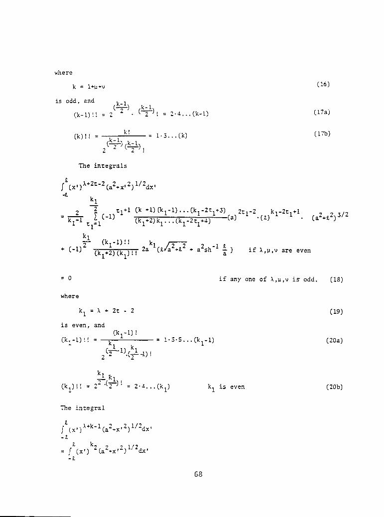
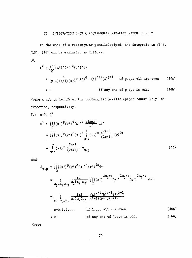
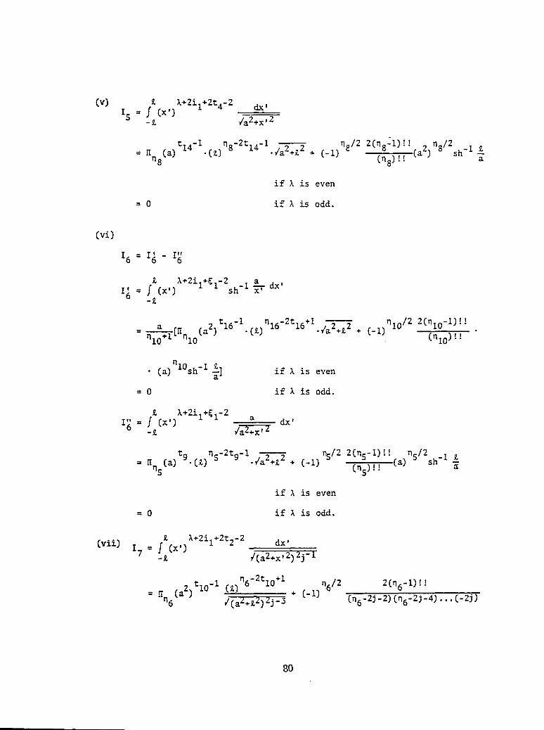
The integrals in (44) can be evaluated as in Appendix B.
75
REFERENCES
[i] L.S. Fu and T. Mura, Volume Integrals Associated with the InhomogeneousHelmholtz Equation: I. Ellipsoidai Region, NASA Contractor Report XXXX,1983.
[2] L.S. Fu and T. Mura, Volume Integrals of an Ellipsoid Associated with
the Inhomogeneous Helmholtz Equation, Wave Motion, !(2), 141-149,{April, 1982).
[3] I.S. Gradshteyn and I.M. Ryzhik, Table of Integrals, Series andProducts, Academic Press, N.Y., 196S.
[4] P.M. Morse and H. Feshbach, Methods of Theoretical Physics, McGraw-Hill,N.Y., 1277, 1953.
77
APPENDIX B
The I-Integrals and r-Functions
(a) The I-integrals
(i) £ %.Zn(bZ.x, tl-i _ _ ,2)3 dx'II : f (x') 2) /(a'.b'.x
(a2.b2)t3-i _-2t_*lF! 2Fl o 2)5= ,n.,[ FI!F2, (b) • -(.t) /',a2+b2.
il,Z2
m
. [ (_z)n/2 :_ 8(n-!)_! "'z - " n/2 - -F1 F,! (n.a)_ (b) .(a'*b _) [_Z-/(a2*b2._:) _ *FI,F2
5. 2 ,2, " ", _ v . _ _.
. Tta -,-o )CZ/a".b"_- - + (a-*b_)si _, ! _)]
if k is even
: 0 if \ is odd
in which zhe _-func=ion-, is defined in (b) of the Appendix.
(_:_ I : il " ""
Z k+2n= .:at[. -(b"'x /_/a--b'_-x'- ix'-£
: _ > : ._ ,(a) Cb) ".(a'-b-" " .(_) "_(a"b"{-) _
'_I_l,e. "1'2"
n!i_ 2( .. 2e. T (-i) . _, n_-l)'' . n_/2(a) Cb) _ _ _" " (a'*b')f , t
- eI.52 (nl-2),!el,e.
Z/a2.b- v 9 v -I Z( ". - . (a'-b-)sh,,'aZ.b 2
if I is even
: 0 if k is odd.
78
£ l+2nII_ = f (x') {b2+x,2) 3_/2sh-i a- dx'
_ /b_+x !?
28 q-+l q3/2= 2 [ e! aCb) i(£) o I e[ t6+l
el,e 2 el!e2! n_+l - y _ el!eo,( ,'7(-i)o el!e2! _" t6= 1
q3-2t6+l(b2)t6-1C _) q_/2 q.-i
.-2t.+l + (-I) o (b) o tg-i Z 2elno o • E)(a)3(b) .
co
+ [ [ (_i)jl (2Ji)! e! 2Jl+l
- -icJi)'C2Ji.l) "e2"el,e 2 jl=2 02i el ' ,,(a)
t7-1 ns-2t7+l(b 2) (£) n.12 (r13-1) !!
(Xn3 (b2+zz)j I_ i * C-i) "_ .(n3-231 +l)Cq3-2j-l),..CS-2jl)
(b)n3cE, j 1,n3(_,) + (-i) i- 2 i _. 2elE tg- T)-)]Cb)
if _ is even
: 0 if _ is odd.
Ciii) £ _+2iI+2t3-2 2I 3 = f (x') /a +x '2 dx'
ts-iC n2-2ts+i/Ca2.Z2) n2/2 2(n2-i)!! _2/2= Eo2(a2) £) 3 . C-i) (02+2)i[Ca2)
£• (£/a2+£2 + a2sh-I E) if X is even
: 0 if _ is odd.
(iv) £ l+2il+_Ish_ iI4 : f (x') __ dx'-£
a - n9-2tlS +I , ? 2 n9/2 2Cn9-i) ![
n9+l[,qn9(a2)tlS i(£) Ca-+_ + (-i) (_9). Ca)ngsh-I a£•_ J
if ,Iis even
= 0 if I is odd.
79
(v3 _IS = f (x,)t+2Xl.2t4 -2 dx'_£ /a2+x, 2
t14-1 n8/2 2(n8-1 )!!= II (a) .(_)n8-2t14-1./a2+£2 + (-1) (a2)n8/2sh-1 !
_8 (n8)!: a
1£ X is even
= 0 if I is odd.
(vi)
16= -
£ X+2il+_l-2sh_l aI_ : f (x') _-r dx'
t16-1 n16-2t16+I nlO/2 2(ni0-i) I!_ a (a 2) .C_) ./a2+£ 2 (-I)
nlo+l[Hnl0 + (nlO)! !
£(a)nlOsh-1 _] if X is even
= 0 i£ k is odd.
£ k+2ii+_i-2I_ = f (X') a dx'
_£ ,/a2+x, 2"
t 9 ns/2 2(ns-i) z:= lI (a) -(£)rls-2tg"l-c'a2+£2 + (-1) (a)nS/2sh-1 £
n5 (n5) I! _r
if I is even
= 0 if I is odd.
£ X+2il+2t2-2 dx'(vii)z?= f (x,)-z /(a2.x, 2)2j- z
tlo-1 (z)n6-2tlO +1 n6/2 2(n6-1) ! !=E (a 2) + (-i)n6 / (a2+£2) 2j-3 (n6-2J-2) (n6-2J-4)... (-2j)
8O
j-2 8k 7ll(j-2)(j-3)...(J-kll-l) (a'. 2)kll
an6Z (i + _ k )
(2j-S)a2/(a2._2)2j -5' kl!=l (2j-S)(2j-7)'''(2j-2kll-5) (4a2) ii
if X is even
= 0 if k is odd.
(viii) £ k+2il+_l-2to-2 (a2+x,2) tOdx ,18= f (x')
-Z /(a2+x, 2) 2j-1
o t12-i+€ I(Z)n7-2t12 .I
11!Q9!n7 €i,€2€1:€2! /(a2+£2)2j-a ¢I,€2 -
n7/2 2(n7-1) !!
(-1) (n7-2j-2) (n7=2 j -43 ... (=2j)
j-2 8k kl
(a2)'q7/2+€I Z (i + [ 13(j_2)(j_3)...(J_k13_l)(a2._2) 3
(2j-3)a2/(a2.Z2) 2j-3 kls=l (2j-S) (2j-7)••.(2j-2k13-3) (4a2)k13
if X is even
= 0 if k is odd.
(ix) £ X+2iI+_i-2 dx'
19=f (x'3_£ /(a2+x,2) 2j-i
= rl (aZ)t12-1(Z)_8-2t12+! + (-i)n8/2 2(n8-I) !!
n8 /(a2+£23 2J -1 (n8-2j-2) (n8-2j-4) ... (-2j)
j-2 8k12(j_2) (j-3) ... (j=k!2 -1) (a2+£-}0 k12an8_ (1 + [ )
(2j-S)a2/(a2+£2)2j -'3 k12=l (2j-S) (2j-7)...(2j-2k12-3) (4a2) k12
if I is even
= 0 if k is odd.
81
(h) The ,_-Functions
The _-ftmctions in the l-integrals listed in Ca) of this Appendix are
defined as follows:
(i) : -_=_?n/2_ (n.l)Cn-i)...Cn-Zt3+3)(-1)r,+l _- (n_-4)C_.,-2)...(n-2t.+6)iIq t3=l
n : I . 2n2 + 21"2 (is even)
F1 . F2 = F : _i-i
(ii) _nl as the same as (35), if replace _ with n1
nI : i . 2n! .292 (is even)
e 1 . e2 = 9 = _/2
(iii)n7/2
2 t7.l (n3+l)(n3-1)'''('q3-2t7+3)zEN3 q.+! (q 3- 2j 1.1) (r]3- 2j.1.1) (q3_Zj 1.217+3)
C-i):7=i •..
Jl-I
)" (_i)t8 ''z (2) t8 -1 [3-2-'(Jf"i)][S-2Jl]'''[S-2(J!-tS"2)]
_q'n3: 3-2(JI+i) t8:l" " (Jl-l)(J1-2)'''(jl-t8)
no_: k . 2nI . 2e?. (is even)
3
el * e2 : e = _ _,
(iv) En2 as the same as (35), if replace _ with n2
n2 = i + 2i! . 2t3 - 2 (is even)
(v) _n9 as the same as (32a), if"replace v with n9
n9 : I + 2ii + _i (is even)
82
(vi) .2 as the same as (32a), if replace _ with q8_8
q8 = \ + 2ii + 2t4 -2 (is even)
(vii) X as the same as (32a), if replace _ with nlOnlO
nlO = '\_ 2ii + gl 2 (is even)
(viii) H as the same as (32a), if replace ,Jwith n.q5
qS = X +2ii " _I -2 (is even)
(ix) _ q6/2 tlo+l (q6_l)(n6-1)...(q6-2tlO+3)
F.'n.: n6+l 7 (-I) (q6-2j-2)(q6-2j-4) 2io tlo=l "''(n6- --2tlo)
q6 = _ _ 2i +2t_- _ (iseven)1
, if replace n6 with n-(x) Hn. as the same as _q6 //
= +2ii _i - - _ (is even)q7 _ + +2¢2 2to
_I + 62 = ¢ = to
(xi) .qn8as the same as _q6 if replace n6 with q8
n8 = .I+ 2i! + _i - -_ (is even)
83
1. Report No. 2. Government Accession No. 3. Recipient's Catalog No.
NASACR-38514. Title and Subtitle 5. Report Date
January 1985Fundamentals of Microcrack Nucleation Mechanics
6. Performing Organization Code
7. Author(s) 8. Performing Organization Report No.
L. S. Fu, Y. C. Sheu, C. M. Co, W. F. Zhong, and RFP763340/714952H. D. Shen 10.WorkUnitNo.
9. Performing Organization Name and Address11. Contract or Grant No.
The Ohio State University1314 Kinnear Road NAG3-340Columbus, Ohio 43212 13. Type of aeport and Period Covered
12. Sponsoring Agency Name and Address Contractor Report
National Aeronautics and Space Administration 14. Sponsoring Agency Code
Washington, D.C. 20546 505-53-1A (E-2296)
15. Supplementary Notes
Final report. Project Manager, Alex Vary, Structures Division, NASALewisResearch Center, Cleveland, Ohio 44135.
16. Abstract
This work identifies a foundation for ultrasonic evaluation of microcrack nucle-ation mechanics. The objective is to establish a basis for correlations betweenplane strain fracture toughness and ultrasonic factors through the interaction ofelastic waves with material microstructures, e.g_, grain size or second-phase par-ticle spacing. Since microcracking is the origin of (brittle) fracture it is ap-propriate to consider the role of stress waves in the dynamics of microcracking.Therefore, this work deals with the following topics: (I) microstress distribu-tions with typical microstructural defects located in the stress field, (2) elas-tic wave scattering from various idealized defects, (3) dynamic effective-proper-ties of media with randomly distributed inhomgeneities.
17. Key Words (Suggested by Author(s)) 18. Distribution Statement
Microcracking; Microcrack nucleation;Ultrasonics; Ultrasonic waves;
Unclassified- unlimitedScattering; Elastic waves; Elasticscattering; Ultrasonic attenuation; STARCategory 38Inclusions; Voids ; Microstructure
19. Security Classif. (of this report) 20. Security Classif. (of this page) 21. No. of pages 22. Price*
Unclassi fied Unclassified 85 A05
*For sale by the National Technical Information Service, Springfield, Virginia 22161NASA-Langley, 1985