Probabilistic Planning 2Probabilistic Planning 2

Nathaniel OsgoodNathaniel Osgood33--2727--20042004

TopicsTopics

PERT (Cont’d)PERT (Cont’d)ReviewReviewMerge node biasMerge node biasPNetPNet refinementrefinement

Monte CarloMonte CarloSimulation approachesSimulation approaches

GeneralGeneralDemoDemoProcess InteractionProcess InteractionActivity ScanningActivity Scanning

PERT BasicsPERT Basics

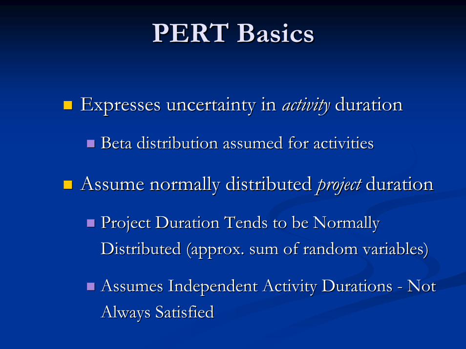
Expresses uncertainty in Expresses uncertainty in activity activity duration duration

Beta distribution assumed for activitiesBeta distribution assumed for activities

Assume normally distributed Assume normally distributed projectproject durationduration

Project Duration Tends to be Normally Project Duration Tends to be Normally Distributed (approx. sum of random variables)Distributed (approx. sum of random variables)

Assumes Independent Activity Durations Assumes Independent Activity Durations -- Not Not Always SatisfiedAlways Satisfied

Stochastic ApproachStochastic Approach

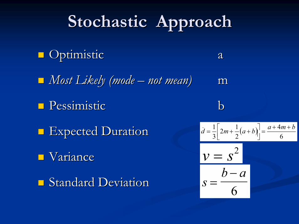
Optimistic Optimistic aa

Most Likely (mode Most Likely (mode –– not mean)not mean) mm

PessimisticPessimistic bb

Expected DurationExpected Duration

VarianceVariance

Standard Deviation

( )6

4212

31_ bmabamd ++

=⎥⎦⎤

⎢⎣⎡ ++=

v s= 2

sb a

=−6

Standard Deviation

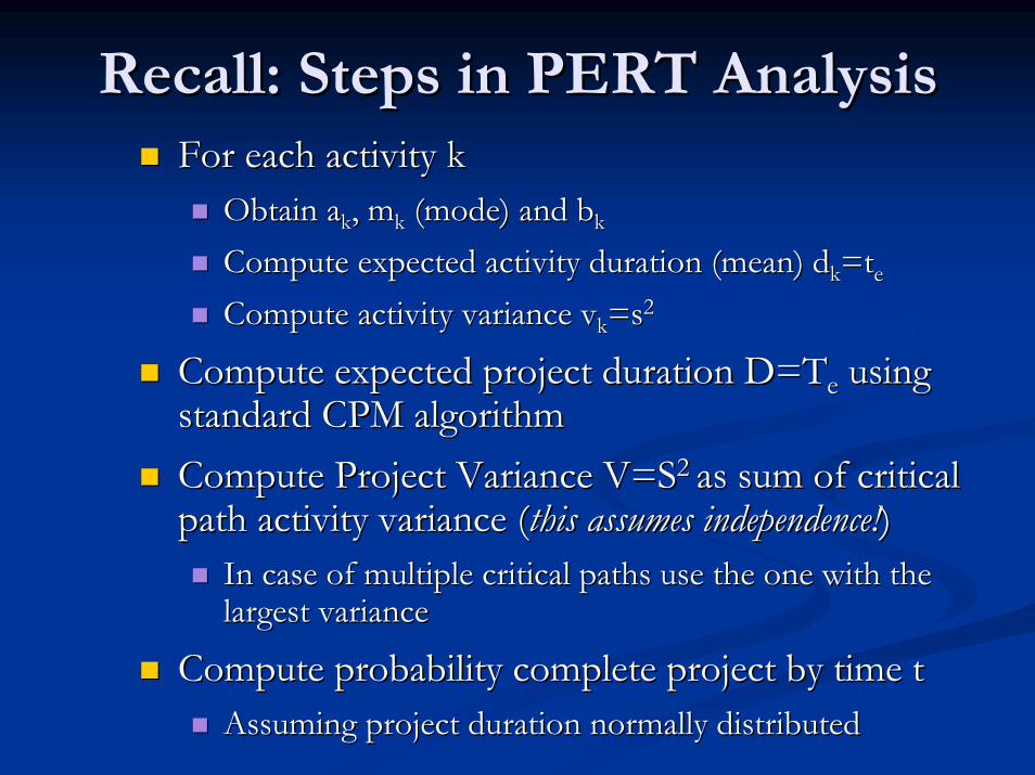
Recall: Steps in PERT AnalysisRecall: Steps in PERT AnalysisFor each activity kFor each activity k

Obtain Obtain aakk, , mmkk (mode) and (mode) and bbkk

Compute expected activity duration (mean) Compute expected activity duration (mean) ddkk==ttee

Compute activity variance Compute activity variance vvkk=s=s22

Compute expected project duration D=TCompute expected project duration D=Tee using using standard CPM algorithmstandard CPM algorithmCompute Project Variance V=SCompute Project Variance V=S2 2 as sum of critical as sum of critical path activity variance (path activity variance (this assumes independence!this assumes independence!))

In case of multiple critical paths use the one with the In case of multiple critical paths use the one with the largest variance largest variance

Compute probability complete project by time tCompute probability complete project by time tAssuming project duration normally distributedAssuming project duration normally distributed

PERT ExamplePERT Example

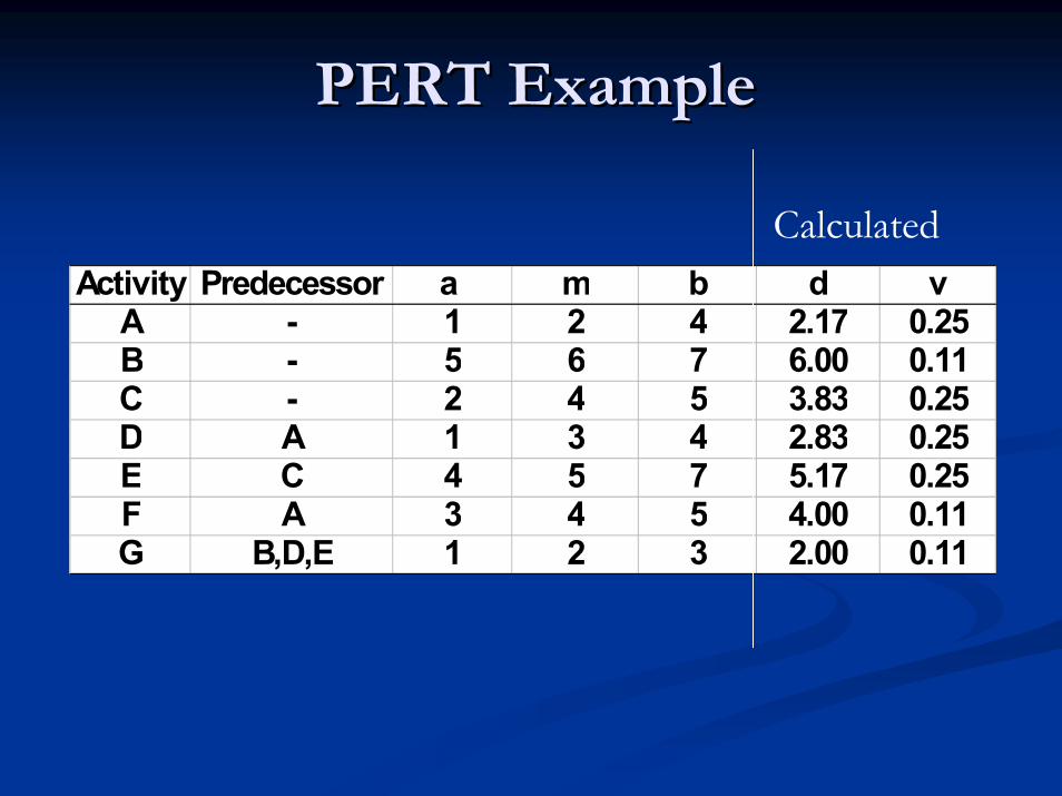
Activity Predecessor a m b d vA - 1 2 4 2.17 0.25B - 5 6 7 6.00 0.11C - 2 4 5 3.83 0.25D A 1 3 4 2.83 0.25E C 4 5 7 5.17 0.25F A 3 4 5 4.00 0.11G B,D,E 1 2 3 2.00 0.11

Calculated

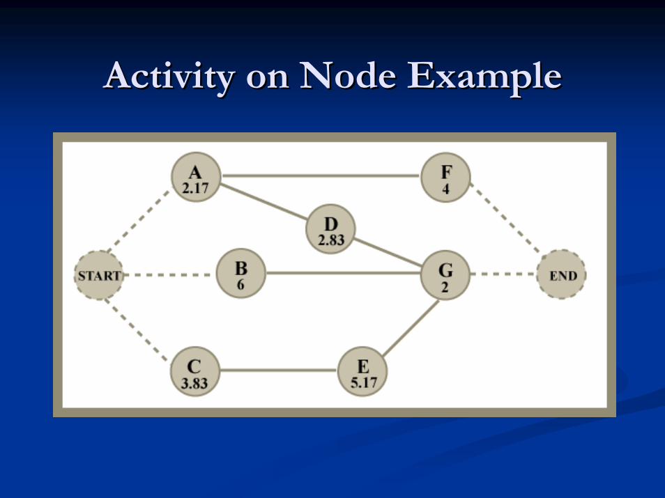
Activity on Node ExampleActivity on Node Example

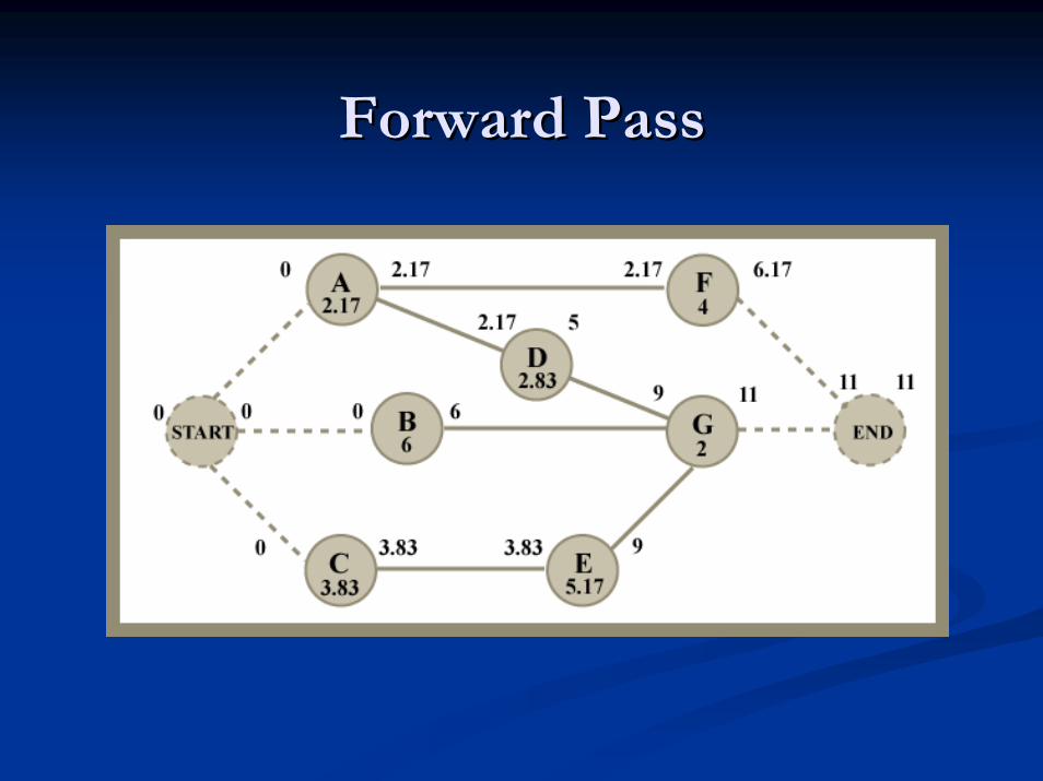
Forward PassForward Pass

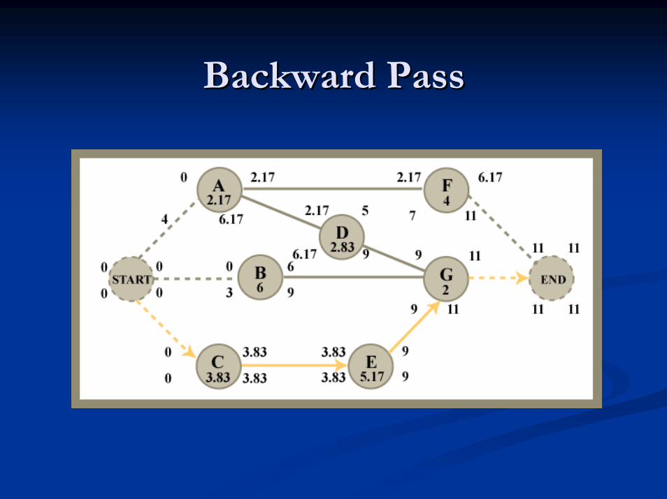
Backward PassBackward Pass

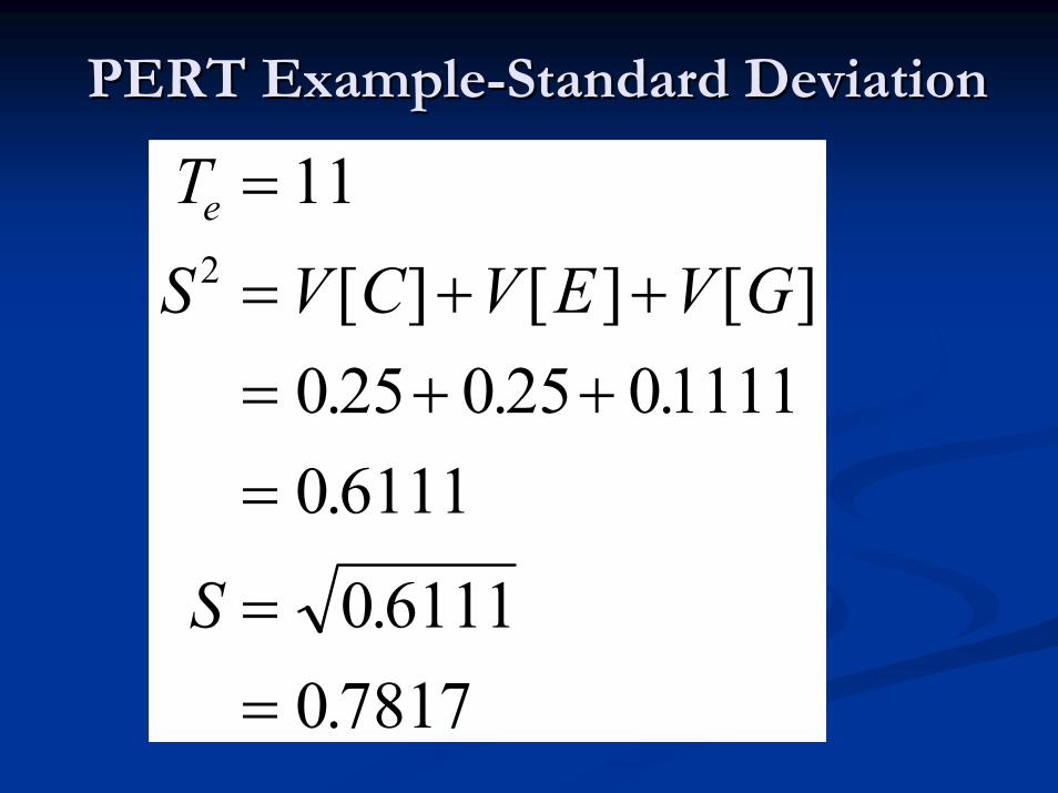
PERT ExamplePERT Example--Standard DeviationStandard Deviation

TS V C V E V G

S

e =

= + += + +=

==

11

0 25 0 25 011110 6111

0 61110 7817

2 [ ] [ ] [ ]. . ..

..

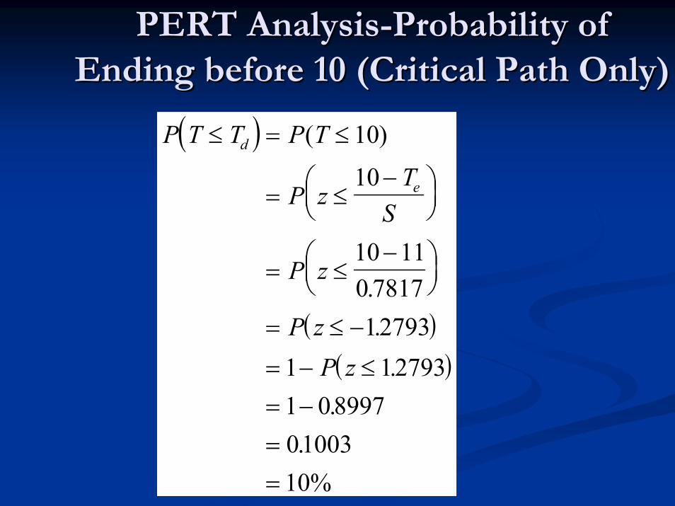
PERT AnalysisPERT Analysis--Probability of Probability of Ending before 10 (Critical Path Only)Ending before 10 (Critical Path Only)

( )

( )( )

P T T P T

P zTS

P z

P zP z

d

e

≤ = ≤

= ≤−⎛

⎝⎜⎞⎠⎟

= ≤−⎛

⎝⎜⎞⎠⎟

= ≤ −

= − ≤= −==

( )

..

..

.

10

10

10 110 781712793

1 127931 089970100310%

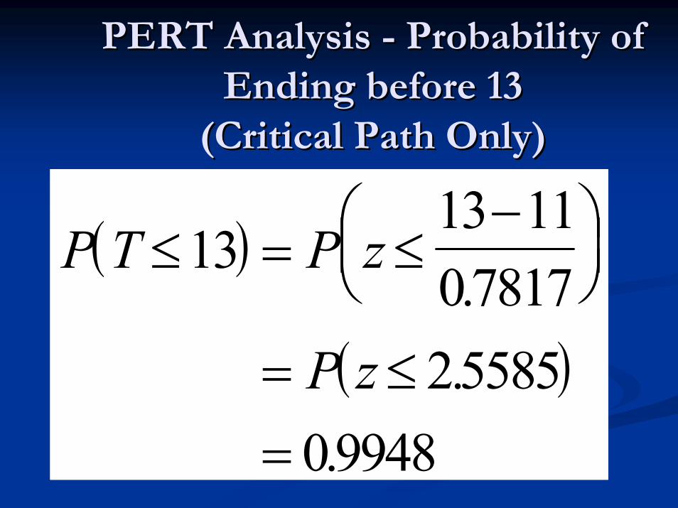
PERT Analysis PERT Analysis -- Probability of Probability of Ending before 13 Ending before 13

(Critical Path Only)(Critical Path Only)

( )

( )

P T P z

P z

≤ = ≤−⎛

⎝⎜⎞⎠⎟

= ≤=

1313 110781725585

09948

..

.

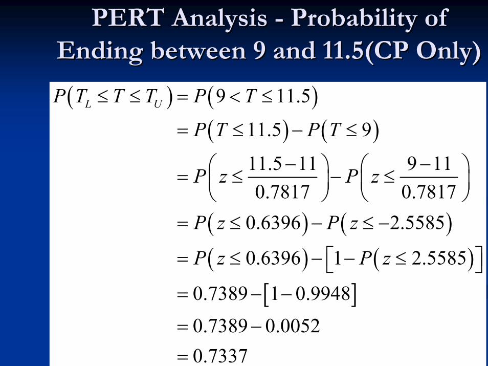
PERT Analysis PERT Analysis -- Probability of Probability of Ending between 9 and 11.5(CP Only)Ending between 9 and 11.5(CP Only)

( ) ( )( ) ( )

( ) ( )( ) ( )

[ ]

9 11.5

11.5 9

11.5 11 9 110.7817 0.7817

0.6396 2.5585

0.6396 1 2.5585

0.7389 1 0.99480.7389 0.00520.7337

L UP T T T P T

P T P T

P z P z

P z P z

P z P z

≤ ≤ = < ≤

= ≤ − ≤

− −⎛ ⎞ ⎛ ⎞= ≤ − ≤⎜ ⎟ ⎜ ⎟⎝ ⎠ ⎝ ⎠

= ≤ − ≤ −

= ≤ − − ≤⎡ ⎤⎣ ⎦= − −

= −=

TopicsTopics

PERT (Cont’d)PERT (Cont’d)ReviewReviewMerge node biasMerge node biasPNetPNet refinementrefinement

Monte CarloMonte CarloSimulation approachesSimulation approaches

GeneralGeneralDemoDemoProcess InteractionProcess InteractionActivity ScanningActivity Scanning

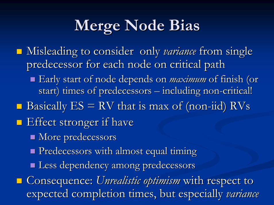
Merge Node BiasMerge Node Bias

Misleading to consider only Misleading to consider only variancevariance from single from single predecessor for each node on critical pathpredecessor for each node on critical path

Early start of node depends on Early start of node depends on maximummaximum of finish (or of finish (or start) times of predecessors start) times of predecessors –– including nonincluding non--critical!critical!

Basically ES = RV that is max of (nonBasically ES = RV that is max of (non--iidiid) RVs) RVsEffect stronger if haveEffect stronger if have

More predecessorsMore predecessorsPredecessors with almost equal timingPredecessors with almost equal timingLess dependency among predecessorsLess dependency among predecessors

Consequence: Consequence: Unrealistic optimismUnrealistic optimism with respect to with respect to expected completion times, but especially expected completion times, but especially variancevariance

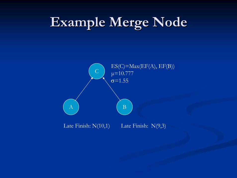
Example Merge NodeExample Merge Node

C

A B

ES(C)=Max(EF(A), EF(B))µ=10.777σ=1.55

Late Finish: N(10,1) Late Finish: N(9,3)

Sample ProblemSample Problem

Derived ParametersDerived Parameters

MEAN AND STANDARD DEVIATION OF THE CRITICAL ANDNEAR CRITICAL PATHS FOR NETWORK

0-3 1 2 3 2 0.39 2 0.39

3-7 6 8 10 8 1.56 - -

7-8 3.5 5 6.5 5 0.88 - -

3-4 1 4 13 - - 5 14.06

4-5 2 4 6 - - 4 1.56

5-8 2 3 4 - - 3 0.39

TOTALS* 15.0 2.83 14.0 16.40

STANDARD DEVIATION - 1.68 - 4.05

ACTIVITYa m b MEAN VARIANCE MEAN VARIANCE

TIME ESTIMATES PATH 0-3-7-8 PATH 0-3-4-5-8

* The mean and variance of the duration of a path is merely the sum of the means and variances of the activities along the path in question; the standard deviation of the path duration is then obtained as the square root of its variance.

(Critical Path)

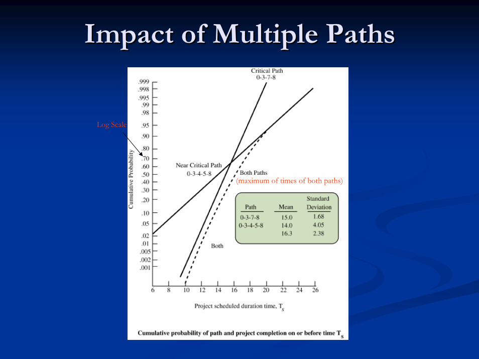
Impact of Multiple PathsImpact of Multiple Paths

(maximum of times of both paths)

Log Scale

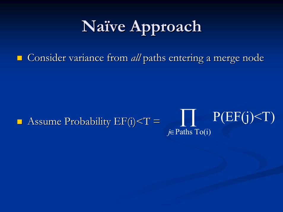
Naïve ApproachNaïve Approach

Consider variance from Consider variance from allall paths entering a merge nodepaths entering a merge node

Assume Probability Assume Probability EF(iEF(i)<T = )<T = Paths To(i)

P(EF(j)<T)j∈∏

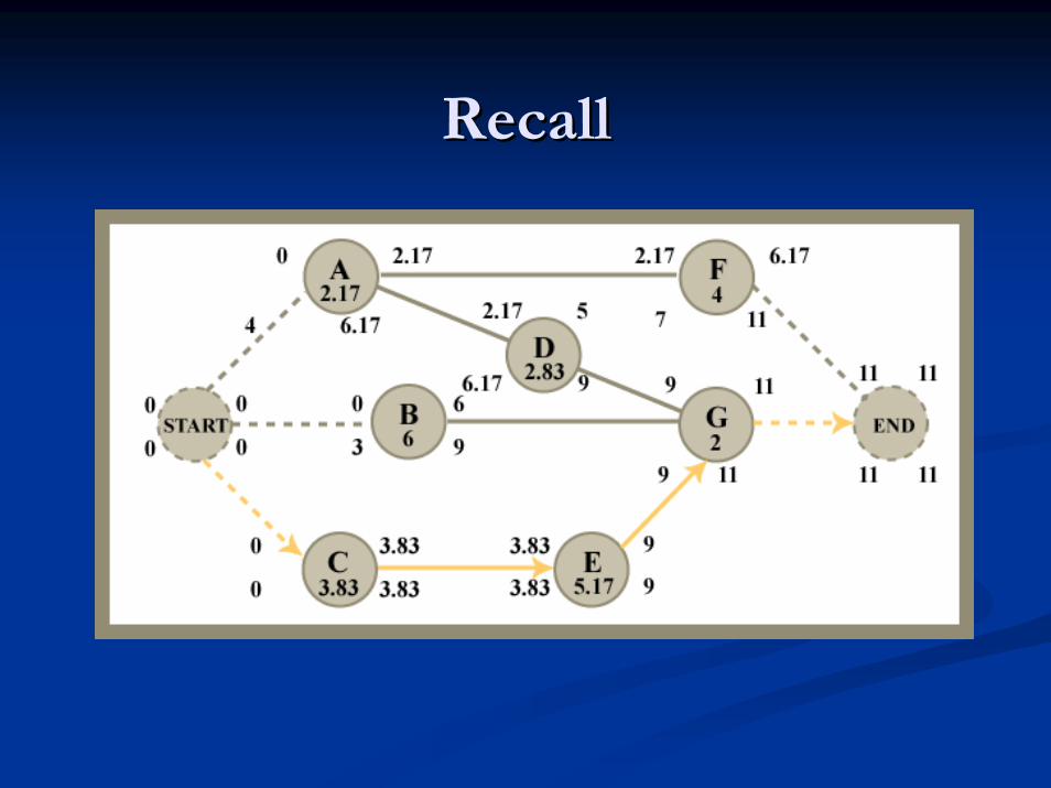
RecallRecall

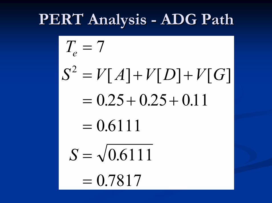
PERT Analysis PERT Analysis -- ADG PathADG Path

TS V A V D V G

S

e =

= + += + +=

==

7

0 25 0 25 0110 6111

0 61110 7817

2 [ ] [ ] [ ]. . ..

..

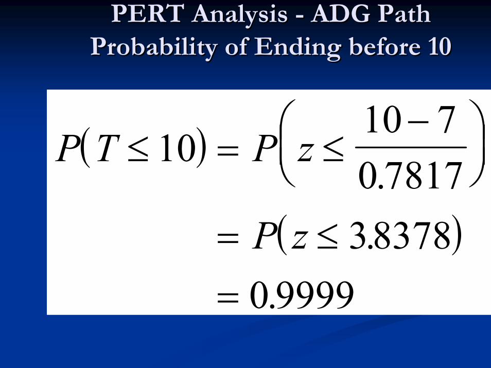
PERT Analysis PERT Analysis -- ADG Path ADG Path Probability of Ending before 10Probability of Ending before 10

( )

( )

P T P z

P z

≤ = ≤−⎛

⎝⎜⎞⎠⎟

= ≤=

1010 70 781738378

0 9999

..

.

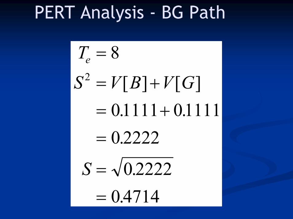
PERT Analysis - BG Path

TS V B V G

S

e =

= += +=

==

8

01111 011110 2222

0 22220 4714

2 [ ] [ ]. ..

..

PERT Analysis - BG Path Probability of Ending before 10

( )

( )

P T P z

P z

≤ = ≤−⎛

⎝⎜⎞⎠⎟

= ≤=

1010 80 47144 2429

0 9999

..

.

PERT Analysis - ADG , BG and CEG Paths Probability of Ending before 10

( ) ( ) ( ) ( )P T P T P T P Tc CEG ADG BG≤ = ≤ ≤ ≤

===

10 10 10 1001003 09999 09999

0100310%

( . )( . )( . ).

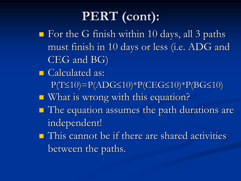
PERT (cont):PERT (cont):For the G finish within 10 days, all 3 paths For the G finish within 10 days, all 3 paths must finish in 10 days or less (i.e. ADG and must finish in 10 days or less (i.e. ADG and CEG and BG)CEG and BG)Calculated as:Calculated as:P(TP(T≤≤10)=P(ADG10)=P(ADG≤≤10)*P(CEG10)*P(CEG≤≤10)*P(BG10)*P(BG≤≤10)10)

What is wrong with this equation?What is wrong with this equation?The equation assumes the path durations are The equation assumes the path durations are independent!independent!This cannot be if there are shared activities This cannot be if there are shared activities between the paths.between the paths.

Example of Multiple Paths Example of Multiple Paths ––Dependent and IndependentDependent and Independent

Activities with duration 2 have σ=.707Activities with duration 4 have σ=1.414

PERT (cont):PERT (cont):A Solution: Use eitherA Solution: Use either

PNetPNetMonte Carlo simulationMonte Carlo simulation

PNetPNet

Aims at addressing merge node biasAims at addressing merge node biasBasically works by Basically works by

Enumerate all paths P Enumerate all paths P s.ts.t. . Dur(PDur(P)> )> ααDur(critDur(crit path)path)Rank paths by decreasing duration (by decreasing naivelyRank paths by decreasing duration (by decreasing naively--estimated variance for ties)estimated variance for ties)Compute linear correlation coefficient between pathsCompute linear correlation coefficient between pathsEnter paths, eliminating any path whose correlation Enter paths, eliminating any path whose correlation coefficient with a previouslycoefficient with a previously--entered path is > .5entered path is > .5

# remaining paths

1

( ) ( )ii

P T a P p T=

≤ = ≤∏

PERT DisadvantagesPERT DisadvantagesValidity of Beta distribution for activity Validity of Beta distribution for activity durationsdurationsValidity of central limit theorem for project Validity of central limit theorem for project durationduration

Activity durations are not independent!Activity durations are not independent!Take into consideration only critical pathTake into consideration only critical path

Not just sum of random variables Not just sum of random variables ---- have max. have max. at joins at joins Leads to Leads to overoptimismoveroptimism & underestimation & underestimation of durationof duration

Multiple time estimates required to calibrateMultiple time estimates required to calibrateCan be time consumingCan be time consuming

TopicsTopics

PERT (Cont’d)PERT (Cont’d)ReviewReviewMerge node biasMerge node biasPNetPNet refinementrefinement

Monte CarloMonte CarloSimulation approachesSimulation approaches

GeneralGeneralDemoDemoProcess InteractionProcess InteractionActivity ScanningActivity Scanning

Monte Carlo Simulation Monte Carlo Simulation CharacteristicsCharacteristics

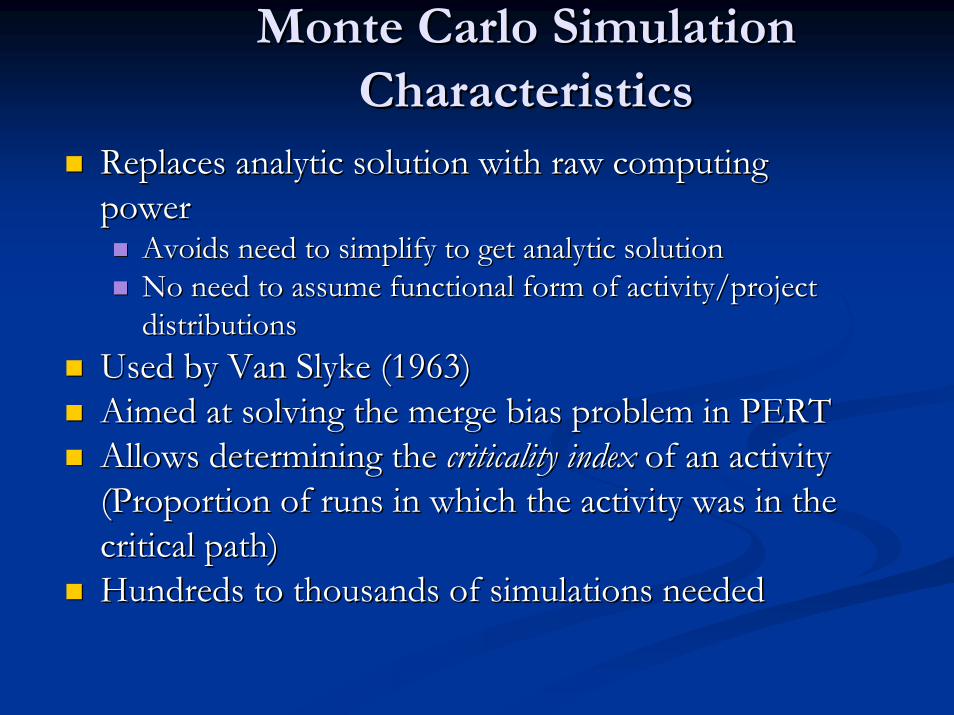
Replaces analytic solution with raw computing Replaces analytic solution with raw computing powerpower

Avoids need to simplify to get analytic solutionAvoids need to simplify to get analytic solutionNo need to assume functional form of activity/project No need to assume functional form of activity/project distributionsdistributions

Used by Van Used by Van SlykeSlyke (1963)(1963)Aimed at solving the merge bias problem in PERTAimed at solving the merge bias problem in PERTAllows determining the Allows determining the criticality indexcriticality index of an activity of an activity (Proportion of runs in which the activity was in the (Proportion of runs in which the activity was in the critical path)critical path)Hundreds to thousands of simulations neededHundreds to thousands of simulations needed

Monte Carlo Simulation ProcessMonte Carlo Simulation ProcessSet the duration distribution for each activity Set the duration distribution for each activity

No functional form of distribution assumedNo functional form of distribution assumedCould be joint distribution for multiple activitiesCould be joint distribution for multiple activities

Iterate: for each “trial” (“realization”)Iterate: for each “trial” (“realization”)Sample random duration from each distributionsSample random duration from each distributionsFind critical path & durations with Find critical path & durations with standard CPMstandard CPM

Record these resultsRecord these resultsReport recorded resultsReport recorded results

Duration distributionDuration distributionPerPer--node criticality index (% runs where critical)node criticality index (% runs where critical)

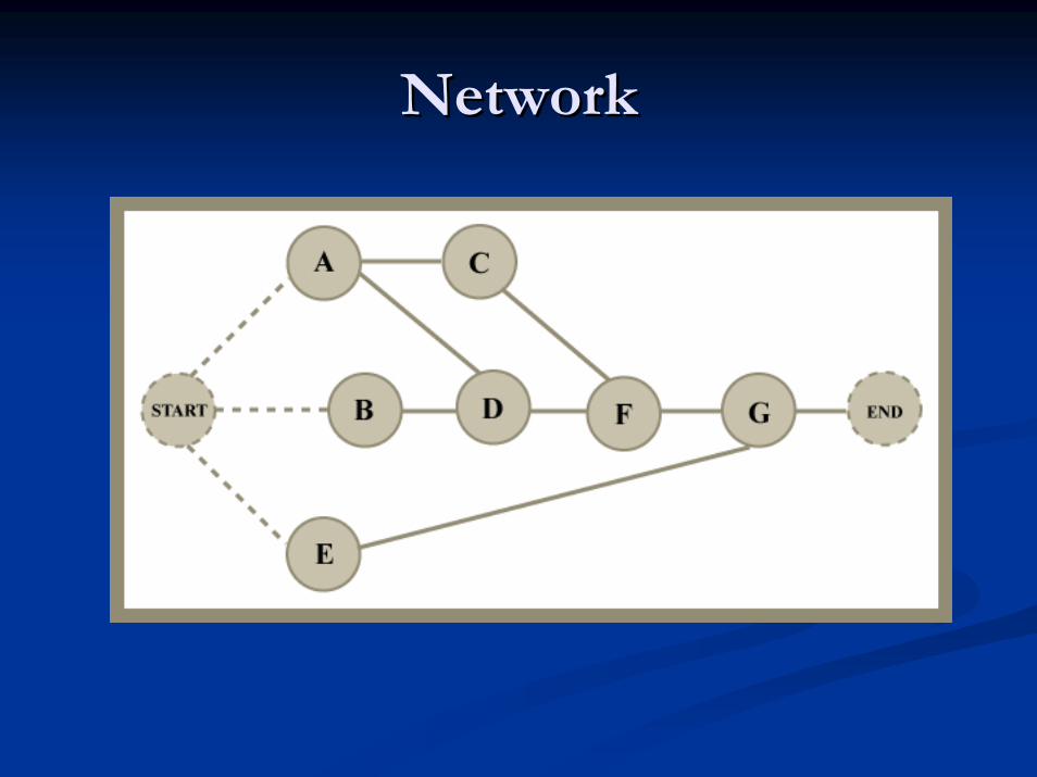
NetworkNetwork

Monte Carlo Simulation ExampleMonte Carlo Simulation Example

Statistics for Example Activities

Activity

OptimisticTime,

a

Most LikelyTime,

m

PessimisticTime,

b

ExpectedVal ue,

d

Stan dardDeviation ,

sA 2 5 8 5 1B 1 3 5 3 0.66C 7 8 9 8 0.33D 4 7 10 7 1E 6 7 8 7 0.33F 2 4 6 4 0.66G 4 5 6 5 0.33

Monte Carlo Simulation ExampleMonte Carlo Simulation Example

Activity DurationSummary of Simulation Runs for Example Project

RunNumber A B C D E F G

CriticalPath

CompletionTime

1 6.3 2.2 8.8 6.6 7.6 5.7 4.6 A-C-F-G 25.42 2.1 1.8 7.4 8.0 6.6 2.7 4.6 A-D-F-G 17.43 7.8 4.9 8.8 7.0 6.7 5.0 4.9 A-C-F-G 26.54 5.3 2.3 8.9 9.5 6.2 4.8 5.4 A-D-F-G 25.05 4.5 2.6 7.6 7.2 7.2 5.3 5.6 A-C-F-G 23.06 7.1 0.4 7.2 5.8 6.1 2.8 5.2 A-C-F-G 22.37 5.2 4.7 8.9 6.6 7.3 4.6 5.5 A-C-F-G 24.28 6.2 4.4 8.9 4.0 6.7 3.0 4.0 A-C-F-G 22.19 2.7 1.1 7.4 5.9 7.9 2.9 5.9 A-C-F-G 18.910 4.0 3.6 8.3 4.3 7.1 3.1 4.3 A-C-F-G 19.7

Project Duration DistributionProject Duration Distribution

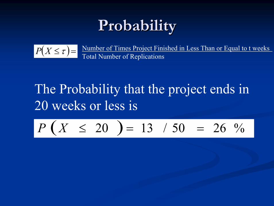
ProbabilityProbabilityNumber of Times Project Finished in Less Than or Equal to t weeksTotal Number of Replications

( ) =≤τXP

The Probability that the project ends in 20 weeks or less is( ) %2650/1320 ==≤XP

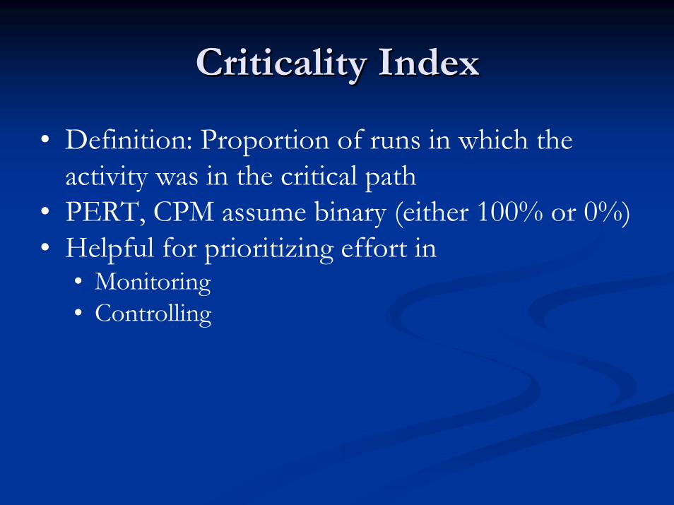
Criticality IndexCriticality Index

• Definition: Proportion of runs in which the activity was in the critical path

• PERT, CPM assume binary (either 100% or 0%)• Helpful for prioritizing effort in

• Monitoring• Controlling

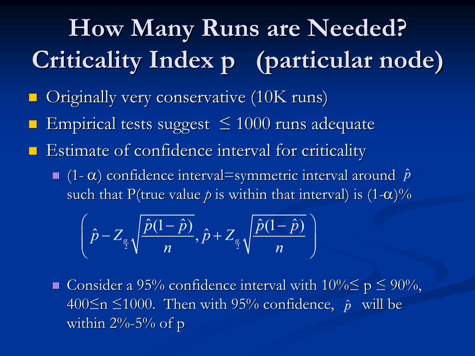
How Many Runs are Needed? How Many Runs are Needed? Criticality Index p (Criticality Index p (particular node)particular node)

Originally very conservative (10K runs)Originally very conservative (10K runs)Empirical tests suggest Empirical tests suggest ≤≤ 1000 runs adequate1000 runs adequateEstimate of confidence interval for criticality Estimate of confidence interval for criticality

(1(1-- αα) confidence interval=symmetric interval around ) confidence interval=symmetric interval around such that such that P(trueP(true value value pp is within that interval) is (1is within that interval) is (1--αα)%)%

Consider a 95% confidence interval with 10%Consider a 95% confidence interval with 10%≤≤ p p ≤≤ 90%, 90%, 400400≤≤n n ≤≤1000. Then with 95% confidence, will be 1000. Then with 95% confidence, will be within 2%within 2%--5% of p5% of p

2 2

ˆ ˆ ˆ ˆ(1 ) (1 )ˆ ˆ,p p p pp Z p Zn nα α

⎛ ⎞− −− +⎜ ⎟⎜ ⎟

⎝ ⎠

p

p

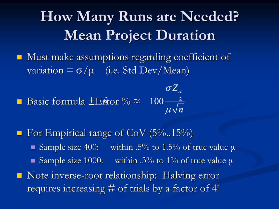
How Many Runs are Needed? How Many Runs are Needed? Mean Project DurationMean Project Duration

Must make assumptions regarding coefficient of Must make assumptions regarding coefficient of variation = variation = σσ//µµ (i.e. Std Dev/Mean)(i.e. Std Dev/Mean)

Basic formula Basic formula ±±Error % Error % ≈≈

For Empirical range of For Empirical range of CoVCoV (5%..15%)(5%..15%)Sample size 400: within .5% to 1.5% of true value Sample size 400: within .5% to 1.5% of true value µµSample size 1000: within .3% to 1% of true value Sample size 1000: within .3% to 1% of true value µµ

Note inverseNote inverse--root relationship: Halving error root relationship: Halving error requires increasing # of trials by a factor of 4!requires increasing # of trials by a factor of 4!

u 2100Z

n

ασ

µ

How Many Runs are Needed? How Many Runs are Needed? Project Duration Standard DeviationProject Duration Standard Deviation

Basic formula Basic formula ±±Error % Error % ≈≈

Sample size 400: within 7% of true value Sample size 400: within 7% of true value σσSample size 1000: within 4.38% of true value Sample size 1000: within 4.38% of true value σσ

InverseInverse--root relationship again presentroot relationship again present

σ

2

100

2

Z

n

α

σ

Monte Carlo: SummaryMonte Carlo: SummaryConceptually simpleConceptually simple

Standard CPM usedStandard CPM usedNo need for special assumptions about functional No need for special assumptions about functional form of distributionsform of distributions

Provides criticality index (valuable prioritization)Provides criticality index (valuable prioritization)Scalable analysis quality (albeit with superScalable analysis quality (albeit with super--linear linear effort required to reduce error) effort required to reduce error) Computationally expensiveComputationally expensiveEstimation of duration distributions can be Estimation of duration distributions can be expensiveexpensive

TopicsTopics

PERT (Cont’d)PERT (Cont’d)ReviewReviewMerge node biasMerge node biasPNetPNet refinementrefinement

Monte CarloMonte CarloSimulation approachesSimulation approaches

GeneralGeneralDemoDemoProcess InteractionProcess InteractionActivity ScanningActivity Scanning

(Dynamic) Simulation Approach(Dynamic) Simulation Approach

CPMCPM--Based methods use simple representationsBased methods use simple representationsOneOne--pass: No iterationpass: No iterationRepresented uncertainty only with respect to Represented uncertainty only with respect to durationduration

Explicitly representing Explicitly representing processprocess brings benefitsbrings benefitsReasoning about process designReasoning about process designIdentifying Identifying emergent behavioremergent behavior (e.g. dynamic bottleneck)(e.g. dynamic bottleneck)Simpler estimation of some uncertaintiesSimpler estimation of some uncertainties

Must be clear about whether representations are Must be clear about whether representations are just just processprocess--level or also level or also projectproject--levellevel

Detailed RepresentationDetailed RepresentationRepetitive processes for which aggregate Repetitive processes for which aggregate representation is not desirablerepresentation is not desirableProcesses where Processes where staticstatic planning is not possibleplanning is not possible

Repetitive processes for which # cycles unknownRepetitive processes for which # cycles unknownScheduling and coordinating complex interactions Scheduling and coordinating complex interactions (Large #s of brief interactions, dependent on timing)(Large #s of brief interactions, dependent on timing)Cases where timing uncertainties change scheduleCases where timing uncertainties change schedule

Cases where individual timing component can Cases where individual timing component can be estimated, but where aggregate stats not be estimated, but where aggregate stats not knownknown

Examples of Repetitive ProcessesExamples of Repetitive Processes

Earth movingEarth movingTunnelingTunnelingHotel/Apartment/Dormitory constructionHotel/Apartment/Dormitory constructionRoad/Bridge constructionRoad/Bridge constructionPlumbing and glazing in highPlumbing and glazing in high--riserise

TopicsTopics

PERT (Cont’d)PERT (Cont’d)ReviewReviewMerge node biasMerge node biasPNetPNet refinementrefinement

Monte CarloMonte CarloSimulation approachesSimulation approaches

GeneralGeneralDemoDemoProcess InteractionProcess InteractionActivity ScanningActivity Scanning

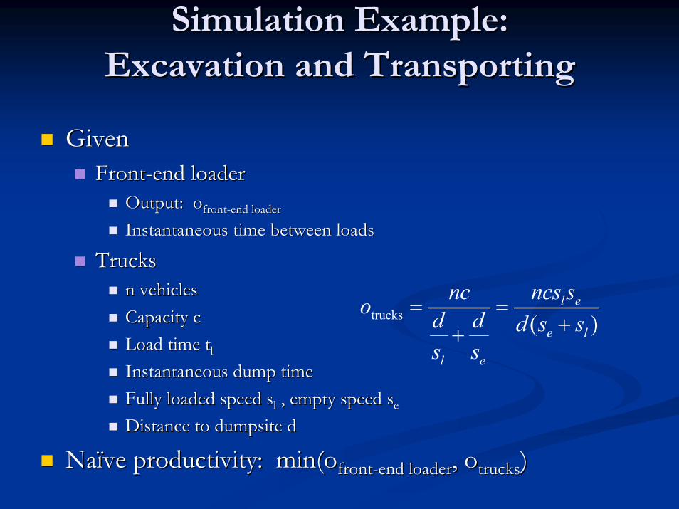
Simulation Example: Simulation Example: Excavation and TransportingExcavation and Transporting

GivenGivenFrontFront--end loader end loader

Output: Output: oofrontfront--end loaderend loader

Instantaneous time between loadsInstantaneous time between loads

TrucksTrucksn vehiclesn vehiclesCapacity cCapacity cLoad time Load time ttll

Instantaneous dump timeInstantaneous dump timeFully loaded speed Fully loaded speed ssll , empty speed s, empty speed see

Distance to dumpsite dDistance to dumpsite d

Naïve productivity: Naïve productivity: min(omin(ofrontfront--end loaderend loader, , ootruckstrucks)

trucks ( )l e

e l

l e

nc ncs so d d d s ss s

= =++

)