— .- .,, . L----- ;., NATIONAL ADVISORY COMMITTEE FOR AERONAUTICS TECHNICAL MEMORANDUM 1293 . APPROXIMATE METHOD OF INTEGRATION OF LAI@NAR BOUNDARY LAYER IN INCOMPRESSIBLE FLUID By L. G. Loitsianskii Translation ‘‘Priblizhennyi Pogranichnogo Matematika i .. ... .. Meted Integrirovania Ur avneniiLaminarnogo Sloia v Neszhimaemom Gaze. ” Prikladnaya Mekhanika, USSR, Vol. 13,no. 5, Oct. 1949. Washington July 1951 ,, :..’.,) .: .!
Transcript
—.-.,, .
L-----
;.,
NATIONAL ADVISORY COMMITTEEFOR AERONAUTICS
TECHNICAL MEMORANDUM 1293
.
APPROXIMATE METHOD OF INTEGRATION OF LAI@NAR
BOUNDARY LAYER IN INCOMPRESSIBLE FLUID
By L. G. Loitsianskii
Translation
‘‘PriblizhennyiPogranichnogoMatematika i
. . ... ..
Meted Integrirovania Ur avnenii LaminarnogoSloia v Neszhimaemom Gaze. ” PrikladnayaMekhanika, USSR, Vol. 13,no. 5, Oct. 1949.
Among all existing methods of the approximate integration ofthe differential equations of the laminar boundary layer, the mostwidely used is the method based on the application of the momentumequation (reference 1). The accuracy of this method depends onthe more or less successful choice of a one-parameter family ofvelocity profiles. Thus, for example, the polynomial of the fourthdegree proposed by ?ohlhausen (reference 1) does not give velocitydistributions closely agreeing with actual values in the neighbor-hood of the separation point, so that in the computations a strongretardation of the separation is obtained as compared with experi-mental results (reference 2). The more-accurate methods employedin recent times (references 2 to 4) assume as a single-parsmeterf~lli~yof profi~e~ the exact So].utions of sane special class offlows with given simple velocity distributions on the edge of theboundary layer (single term raised to a power, linear function).
The transition to the more complicated two- and more-parameterfawilies of profiles would require, in addition to the momentume.~u.ation,the employment of other possible equations (for example,the equations of energy (reference 5) and others (reference 6)).A greater accuracy might also then be expected fcr relatively simplevelocity profiles that satisfy only the fundamental boundary con-ditions on the surface of the body and on the edge of the boundarylayer. This second approach, however, as far as is known, has notbeen considered except for very simple solution for the case ofaxial flow past a plate (reference 7).
In the present paper, a solution is given of the problem ofthe plane laminar boundary layer in an incompressible gas; themethod is based on the use of a system of equations of successive
moments (including that of zero moment, the momentum equation) ofthe equation of the boundary layer. Such statement of the problem
l!pribli~he~yi~yetodIntegrirov~ia Uravnenii Laminarnogo po~ra-._nichnogo Sloia v NeszhiriaemomC-aze.” Prikladnaya !4atematikai 14ek-hanika, USSR, Vol. 15, no. 5, Oct. 1949, p. 515-525.
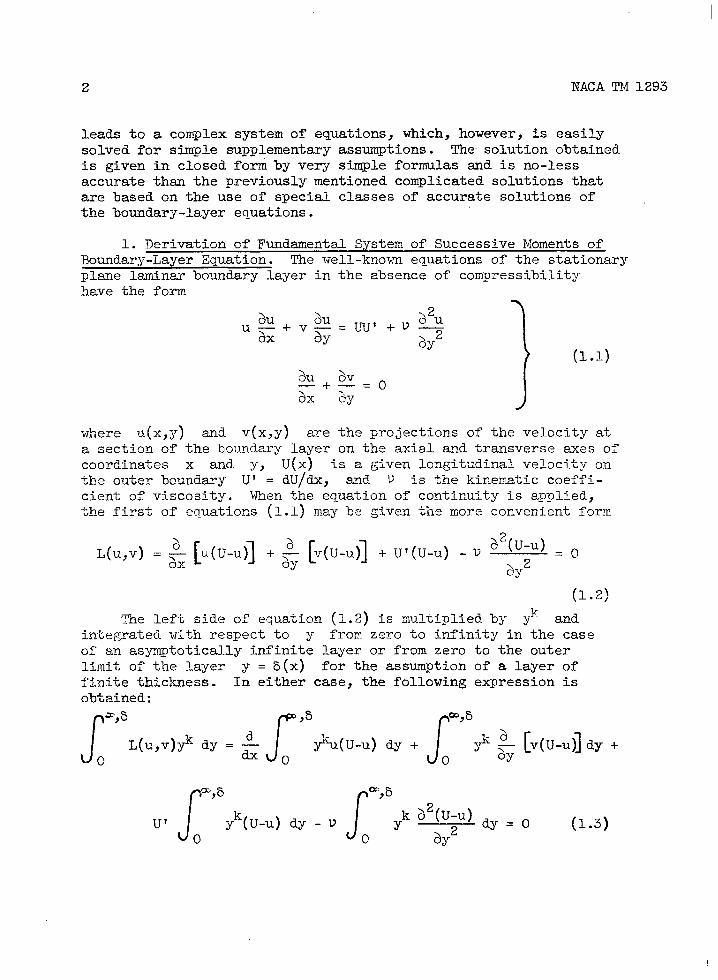
complex system of equations, which, however, is easilysimple supplementary assumptions. The solution obtained
is given in closed form by very simple formulas and is no-lessaccurate than the previously mentioned complicated solutions thatare based on the use of special classes of accurate solutions ofthe boundary-layer equations.
1. Derivation of Fundamental System of Successive Moments ofBoundary-Layer Equation. The well-kno’wnequations of the stationaryplane laminar boundary layer in the absence of compressibilityhave the form
2?h.1 au au
‘s+v F=wJ’+u#
1 (1.1)
where U.(x,y) and V(X,y) are tine projections of the velocity ata section of the bo’J.ndarylayer on the axial and transverse axes ofcoordinates x and y, U(x) is a given longitudinal %“elocityonthe outer hounda~y U’ = dU/dx, and U is the kinematic coeffi-cient of v~.scosity. When the equation of continuity is applied,the first of equations (1.1) may be given t’hemore convenient form
andint~~rated ~’fi~hresPect to y frov.zero to infinity in the caseof an asymptotically im”inite layer or from zero to the outerlimit of the layer y = b(x) for the assumption of a layer offinite thickness. In either case, the following expression isobtained:
J
=,~
[
,8 -,6
L(u,v)’} dy = $ #u(U-u) dy +J
# ~ [v(U-ujjdy +o 0 0 ay
u’J
yk(u-u) &y - uJ
yk~2(U-u) dy _ o
0 0 ayz -
(1.3)
NACA TM
Itview ofto zero
1293
is assumed in this equation and in what follows that, inthe very rapid approach of the velocity difference U -uas. y-+m, all integrals with the infinite upper limit ‘have
a finite value.
For k = O,
J’
*6
r
,5
dGo
u(U-U) dy + U’ (U-u) dy=+o
where the magnitude
(1.4)
(1.5’)
represents the friction stress on the surface of the body.
Equation (1.4), the well-known impulse or momentum equation,is readily-transformed into its usual form-
@H$ + ul&(—— (2+H) =T~dx u pu
where
‘*=Jo(’-:)dypv,b
‘*’JO a+”
(1. s)
1(1.7)
For k = 1, a new equation of the ‘first moment’ is obtainedfrom equation (1.3)
;J5Ju(u-uy+u1Jm’’(1.8)
and, in general, for kz 2, the equations of successively increas-ing moments are obtained
s
=,b
J
-6
r
)Y
d,kU.(U-U) d, - k #-%(U-u) dy+U’G #(U-u) d,
o 0 0
I
,5
= k(k-l)v +2(.-u) dy (1.9)o
In all these equations, the transverse velocity v(x,y) isassumed e~ressed in terms of the axial U(X,Y) from the equationof continuity.
It is now assumed that the family of functions
u=tiO(x, y;~@~, . . . ,Ak) (1.10)
satisfies the boundary-conditions of the problem with k param-eters Al, . . . , hkj which are functions of x, such that the
k successive moments of equation (1.3)
r-,6j3L(u0, VO) dy (1.11)Uo
become zero. On the assumptionthe limit 1{-~~, it would then
u(x,Y) = lim u“ [x, y;~.-+=
that it is permissible to pass tcbe possible to state that the function
~(& A~(x), . . . ,Ak(x]
(1.12)
with parameters Al(x), h2(x), . . . , Ak(x) satisfying the infinites:;stemof e~,uations
5
r*,EJ ;*L(uO, V“) dy = O (k = 0,1, 2,...)
G. . . . .
or, what is equivalent, system. (3..4),(1.El),and (1.9) will be emexact solution of the fund~tientalsystem (1.1) for the assumedboundary conditions.
For this solution, it is merely necessary to recall the knowntheorem that a continuous function, all successive derivatives ofwhich are equal to zero, is identically equal to zero (reference 9).
:?.,i.“f:, The question of the proof’of the validity of this theorem isy
not considered in the case of an infinite interval or of an inter-val the boundaries of which are functions of a certain vsriablewith respect to which the differentiation is effected. A certainconstruction, not based it is true on a rigorous proof, of theso~lltion~jfthe n~-oble~.~,~illl)ee~.pl~yedwith the aid of the Suc-cessive eq~~ationsof the moments of the basic boundary-lajerequstiov..
2. Choice of l’arametersof Family of VelocitjrProfiles at Sec-tions of Bcmmdsry Layer. Special Form of Equations of Moments.As is seen from the previt;uslydiscussed considerations,the funda-mental difficulty lies in the choice of a family of velocity pro-files (1.10) and the determination cf the parameters Ak of thefamily. One of the simplest methods of the sol~tion of this prob-lem is indicatecl.herein.
In the converging part of the “coundarylayer, the velocitypi-ofilesat various s>ctions of tinelayer are kno~ to be almostsifi-dlar;the velocity profile is deforr,edmainly in the diffuserpart Gf the boundary layer downstream of the point of minimum pres-sure. The deformation of the profile consists of the appearanceof a point of flexure tlnatarisss near the surface of the body snd.then moves awaj~from it as the separation point is approached.
The presence of this deformation of the profile nesr the sur-face should greatly affect the magnitude Tll proportional to the
,, normal derivative of the velociti~-on the surface of the bocj.yjitwill therefore diminish to zero as the point of separation is
,, appi-oached. The deformation of the profiie will have a smallereffect on such integral magnitudes as ~+. 6** zpd Ve?y?r.d
- little ef’feet.cn magnitutiesth~t ccntaln under the :ntegralsl.gnf’unlctj,cmt.hetrapidly decreasa as the surface of’‘tkL~ “t:ciy
is z.pprc~.che2.
6 NACA TM 1293
For the parameters characterizing the effect of the deforma-tion of the velocity profile, it is natural to assume those magni-tudes that depend relatively strongly on the deformation of thevelocity profile. ~Jithregard to the magnitudes that vary littlewith the deformation of the velocity profile, however, it is naturalto assume that they do not depend on the chosen pszameters.
For the fundamental parameters determining a change in theshape of the velocity profiles> which may be called form psrsmeters,the nondimensional combination of the magnitudes Tw, 5* and 5**will be er.ployed‘tiththe given functions U(x) and U’(x) andphysical constants, ncunely,the parameters
f = u’5**2v
1
()Tw~**
{=2m-a(y/5**) y=~ ‘--m--
/
(2.1)
JFor the computation of the remaining magnitudes in the equa-
tion of moments according to the assumption, the velocity profilewill,be assumed in a section of the boundary layer in a form thatdoes not depend on the parameters f, ~, and H:
u
()–=9* ‘v(v)‘J
(2.2)
This assumption permits, as will be subsequently seen, obtain-ing on tinebasis of very simple computations a sufficiently accuratesolution of the bcmndsry-layer equations for arbitrary distributionof the velocity on the edge of the layer. The transformation ofequation (1.6) will now he considered.
If the parameter ~ is introduced, then by equation (2.1),
m
R!/j!//;,,f
NACA 9341293
It is not difficult to obtain finally
+~~+f+’-%)f=c ‘2*3)
For the transformation of the left side of equation (1.8)the first integral canbe writtenby equation (2.2) (q = y/!54)
J@yu(u-u)
0
where the magnitude ~17 equal to
(2.5)HI =
J
7T(1AT) dq
o
represents a constant computed by the given function Q(7).
In order to compute the following integral, the transversevelocity v is first expressed by the formula
“=-l’y~dy=-+l’+
8 NACA TM 1293
There is thus obtained
or
(2.7)
1(2.8)
Finally, the last integral in equation (1.8) is transformed into
13ysubstituting the integrals obtained in equation (1.8),
or by replacing &+2/V . f/U’ by equationthe tranafomation,
When the new constants
a=
b=
1(2H1+H3+E4)f +
are introduced,
1
H1 -~H~
2H~+H3+H4
H1-~ H2
the equation of the first moment is reduced
df _ ~ (a-bf) + $ fx-u
(2.11)
(2.1) and carrying out
(2.12)
(2.13)
to the form
(2.14)
The third equation is obtained from the system (1.9) by settingk=2.
There is obtained, as before,
Jy2u(U-u)dyo
(2.15)
s H5U25**3 (2.16)
10where the constant I& IS equal to.
J
:0
H5 = ~zq(l-q)d~o
Further, by analcgy with equation (2.7)
J
w
yv(U-u)dy = H6U28-2 ~ - H7UU‘5*3o
where
I?ACATM 1293
(2.17)
(2.18)
(2.19)
The last integral on the left side of equation (2.15) is equalto
!y2(U-u)dy = H8U b*”x5
o&3=f,2,+ (2.20)
The integnl in equation (2.15) on the right reduces to theunkaown parameter H
By substituting the expressions obtained for the Integrals inthe second-moment equation (2.15), there is obtained, after simpletransfomati ens,
(2.22)
lIACATM 1293 11
The system of t’hreeequations (2.3), (2.14), and (2.22) hasthus been established for deteminlng tke three unknown magnitudes f,~, and H. .The.solution cf this system is now considered.
3. ~~t~rmimtion of the Constants Hi. Approximate Formulasfor ~arameter~ f ~ and H. For the determination of the numeri-cal values of the constants Hl, H2, . . ., H8, the form of thefunction ~ (q) must be known. The simplest velocity profile inthe theory of the asymptotic boundary layer is the velocity profilein the sections of the boundary layer of the flow past a plate.Tinefunction q(q) for this case can easily be determined fromthe generally known table of values of the velocity ratio u/U asa fuaction of : . Y~~/2 .
Super’fluou.scomputations may be avoided by noting that the con-smnbs to be computed are connected with one another by certainsimple relations.
First of all, frGm equations (2.3) and (2.14),
(3.1)
3jTsetting f’. G, there is obtained a . 2~0, where CO
denotes the ragnitude ~ ccmputed for the plate (U’ = 0, f = O).From tha definition of ~ and from the known relations for theplate,
(3.2)
Further, by coinpari~ with one another the magnitudes HI, H2,H3, and H4,
H3.H~-H2 (3.3)
(3.4)
12 N4CA TM 1293
where Ho is the value of H for f . 0, that is, the ratio IS*/5~
for a plate is equal, as is known, to
8* 1.721Ho= w=___= 2.590.664
It is then easy to obtain the value of b by equations (2.13),(3.3), and (3.4).
\Jhen df/d~ is eliminated from equations (2.22) and (2.14),
H . (H5+H7+ $8) f + 3H5-2H5 [1 - (2H1+H3+H4) f]4(H1-; Hz)
(3.6)
By setting f . 0,
‘o~ (3H5~2H6) . ~ . ~ %5.89 (3.7)
The only magnitude that must be computed again from the tableof values q(v) is the magnitude H5 + H7 + H8/2. Numerical inte-
gration gives
H5+H7++H8 = 24.73 (3.8)
after which there is immediately obtained
H = 2.59 - 7.55 f (3.9)
NACA TM 1293 13
Substituting this
t =
expression for H in equation (3.1) gives
0.22 + 1.85 f - 7.55 f2 . (3.10)
*.= ‘Fin&lQ”,‘integratingthe simple linear eg,u&tion(2.14) gives
(axP
faU’
J
~b-l(g)dg
_ 0.44U’
J
U4.5‘~ (E)M
o735.5
0(3.11)
Equations (3.9), (3.10)
The simple, approx~tewith the actual values. Theues of f obtained with theally the only one that is applied)of the preceding works (refer-ences 2 and 3) will be noted. The closed-form relation between ~and f likewise differs little from the correspondingtabulatedfunctions in the references cited.
and (3.11) gfve the required solution.
solution just obtained is now comparedalmost complete agreement of the val-first approx-tion (which is practic-
For comparison, the curves ~(f) and H(f) obtained accord-ing to the formulae of reference 2 and by the formulas (3.10) and(3.9) are shown in figure 1. The results obtained will also becompared with the formulas of Wright and Bailey (reference 9). Anapproximate method of computation of the laminar boundary layer isproposed therein In which the equation of momentum (1.6) is employedwith Tw and 5- substituted by the formulas for the flow pasta plate. By expressing the results of Wright and Bailey In theparameters of the present report, the analogs of equations (3.9),(3.10), and (3.11) are obtained.
H = 2.59)
g = 0.22 + 4.09 f}
(3.12)
JIt is easily seen that this formula for f corresponds to
equation (3.11) for b = 1. The straight lines for ( and Hshowu dotted in figure 1 indicate the considerable deviation ofthe formulas of Wright and Bailey from more accurate formulaspresented herein.
—
14 NACA TM 1293
For confirmation, the particular case of the laminar bountiylayer corresponding to the so-called single-slope velocity distri-bution at the outer boundary of the layer U = l-x will be con-sidered. This case has been theoretically solved and an exactsolution in a tabulated form (reference 10) is available. Theresults of the recomputation of these accurate solutions in theform assumed by the parameters-are given in figure 2. Also shownfor comparison are the corresponding curves obtained by the pro-posed approximate method and by the method of Wright and Bailey.
4. Possible Methods of Render~.ngthe Foregoing Solution MoreAccurate. The method described in the preceding sections was basedon the assumption of a slight dependence of Hi on the form param-
eters f, ~, and H. This assumption may be eliminated and themethcd rendered more accurate, although it thereby becomes con-siderably more complicated.
In order to discuss the possible generalizations of the method,the complete system of equations, for example, for the three-parameter case is written out; that is, a three-parameter familyof velocity profiles is assumed in place of equation (2.2).
(4.1)
By substituting this velocity profile in the system of thethree equations of successive moments (1.6), (1.8) and (2.15),there is obtained a system of three ordinary nonlinear differentialequations that determine the magnitudes of the parameters f) Csand H:
---+(waf+’f=’l~df2 Ur dx
u,=—
u[1 - (2H1+H3+H4)f]+$ (H1-~H2) f
(4.2)
(4.3)
(4.4)
in which, in additfon to the previous notations, the following
(4.5)
15
Ill –..
16 l’?ACATM 1293
It is noted that, in the systemof equations (4.2), (4.3),and (4.4), Hi and Ki are not constant magnltudea Y as pre-
viously, but known functions of the form Parroters f, {,,and H;the form of these functions depends on the chosen family ofprofiles (4.1).
The equations (2.3), (2.14), and (2.22) earlier employed evi-dently represent a particular case of the system (4.2), (4.3), and(4.4) on the assumption that the family of velocity profiles atthe different sections of the boundary layer has the form of equa-tion (2.2); in other words, these profiles are similar to oneanother. All values of Ki are of course then equal
Hi is constant=
The proposed methcilmay be rendered considerablyby assuming, for example, the single-parameterfamilyprofiles
which represents a generalization of equation (2.12) where equa-tion (4.1o) approximates equation (2.12) because of the small changein Hi with change in the parameter f and the smallness of the
magnitude (Kl+aH1/af)f in comparison with Hl - H2/2. This gen-eralization permits obtaining the integral of equation (4.10) byintroducing a correction to the solution of equation (2.12).
By dividing both sides of equation (4.Q) by the correspondingsides of equation (4.8) and thus eliminating df/dx, there isobtained
H . (H5+H7+* H8)f +
[1 - (2Hl+H3+H4)f] +
-[( )( ;~~~ (3H5-2H6) + K4+–Uu,,
HI-*H2U12
~H2 ‘k’+=? ‘ ‘i “H5-2H6)]f ~
Hl --
(4.11)
By similar considerations on the smallness of the magnitudes(K4+l/2 aH5/*)f in comparisonwith (3H5-2H6)/4 and of
(K~+aH@f)f in comparison with HI - H2/2 and on the slightvariability of Hi, it may be concluded that the value of Hdetermined by equation (4.11) is an improvement in the accuracy ofthe approximate value of H according to equation (3.6).
It may be remarked that in this more accurate approximationthere is no longer that universal relation between the parameters Hand f, independent of the form of the function U(x), character-izing the given particular problem. The presence in equation (4.11)
I--——.. . ....—- .-... .—..--— — —
18 NACA TM 1293w
of a second term with the factor UU’’/2’2 shows that in the moreaccurate ayproximatiorithe magnitude H in a given section of thelayer depends not only on the value of the form parameter f inthis section, as was the case in the rougher approximation of equa-tion (3.5) or (3.9), but also on the value of the nmgnitude UU’’/2’2in the section considered, that is, on the values of the func-tion U(x) and its first two derivatives. It is readily observedthat the second term on the right side of equation (4.11) willgive a small correction to the solution (3.6) for relatively smallvalues of the magnitude ~*1/ut2*
The same considerations hold for the expression for ~, whichmay be obtained by substituting df/dx from equation (4.10) andH from equation (4.11) Into equation (4.7):
Zf
[
1 ( @ ‘!+~ (3H5-2H6)f +K4 +-+24
+ (H5+H7+ * H8)f2-
uu4G:)f2[i+‘3H5-2H6)51-(K:+s9(H1-iHJf3u?’ ( HI
HI -~H2+Kl+
(4.12)
As is seen, in this new approximation, in contrast to the pre-ceding ,one,there is no universal relation ~etween { and f. Thepresence of a term with the factor UU’’/U’ makes the magnitude ~depend not only on the value of the parameter f but also on theform of the function U(X) and its first two derivatives in thegiven section of the boundary layer.
It ii of interest to remark that in this approximation theposition of the point of separation of the boundary layer, that is,the value of x = xs for which ~ is equal to zero, will nolonger be determined by some un~versal value of the form parem-eter fs, but in each Individual case the value of x = xs must
be determined for which the right side of equation (4.12) becomeszero.
NACA TM 1293
By assuming a particular form of a family of velocity profiles(4.6), employing, for example, the sets of velocity profilesapplied in the previous investigations (references 2 to 4), thevalues of the functions Hi and Ki are determined; the form
Ptiameters f, ~, and’ H, that is, the thickness of the momentumloss 8-, the friction stress ~w and the displacement thick-
ness” 8* may thenbe found without difficulty. The solutionof equation (4.10) and the determination of H and C by equa-tions (4.11) and (4.12) offers no particular difficulty. Furtherimprovement in the accuracy requiring the solution of a system ofthe type of equations (4.2), (4.3) and (4.4) is hardly of practicalinterest.
In the previous discussion, the scheme of the asymptoticallyinfinite boundary layer was used, but similar equations may beobtained also for the case where the boundary layer is assumed tobe of finite thickness.
The method here proposed may evidently also be applied to thecase of the thermal boundary layer. The characteristic feature ofthe method for the cases of both the dynamic and the thermal bound-ary layer lies in the fact that the friction stress and the quantityof heat given off by a unit area of the body are expressed in inte-gral form and not in terms of the derivatives of functions thatrepresent the approximate velocity and temperature distributionsin the sections of the boundary layer.
Translated by S. ReissNational Advisory Committeefor Aeronautics.
REFERENCES
1. Loitsianskii, L. G.: Aerodynamics of the Boundary Layer.G’ITI,1941, pp. 170, 187.
2. Loitsianski.i,L. G.: Approximate Method for Calculating theLaminar Boundary Layer on the Airfoil. Comptes Rendus(Doklady) de l’Acad. des Sci. de L’URSS, vol. XXXV, no. 8,1942, pp. 227-232.
19
3. Kochin, N. E., and Loitsianskii,L. G.: An Approximate Methodof Computation of the Boundary Layer. D&lady AN SSSR,T. HXVI, No. 9, 1942.
,..
20 , NACA TM 1293,,
...- ,“
4.,~Melnikov,,A.P.:,>
On Certain Prol?le”msin the Theory of a jiin’gin , :.,,a Nonideal Medium. Doctoral dissertation, L. Voenno-vozdushnaia inzhenernaia akademia, 1942v. “. ,,
5. Leibenso”n,L. S.: Energetic Formof the Integral Condition In ~the Theory of the Boundary Layer. Rep. No. 240, CAHI, 1935.
6. Kochin, N. E., Kibei, I. A., and Roze, N. V.: TheoreticalHydrodynamics, pt. II. GTT1, 3d cd., 1948, p. 450.
7. Sutton, W. G. L.: An Approximate Solution of the Boundary LayerEquations for a Flat Plate.’ Phil. Msg. and Jour. Sci.,vol. 23, ser. 7, 1937, pp. 1146-1152.
8. Cerslaw, H., and Jaeger, J.: Operational Methods in AppliedMathematics. 1948.
9. Wright, E. A., and Bailey, G. W.: Laminar Frictional Resistance ‘with Pressure Gradient.
,“Jour. Aero. Sci., vol. 6, no. .12,
Oct. 1939, Pp. 485-488.
10. Howarth, L.: On the SolutionEquations. Proc. Roy. Sot.Feb. 1938,PP. 547-579.