Working Paper 17454http://www.nber.org/papers/w17454
NATIONAL BUREAU OF ECONOMIC RESEARCH1050 Massachusetts Avenue
Cambridge, MA 02138October 2011
Special thanks go to Daniel Green and Hoai-Luu Nguyen for outstanding research assistance. Theauthors also thank Paolo Angelini, Gadi Barlevy, René Carmona, Stephen Brown, Robert Engle, MarkFlannery, Xavier Gabaix, Paul Glasserman, Beverly Hirtle, Jon Danielson, John Kambhu, ArvindKrishnamurthy, Burton Malkiel, Maureen O'Hara, Andrew Patton, Matt Pritsker, Matt Richardson,Jean-Charles Rochet, José Scheinkman, Jeremy Stein, Kevin Stiroh, René Stulz, and Skander Vanden Heuvel for feedback, as well as seminar participants at numerous universities, central banks, andconferences. We are grateful for support from the Institute for Quantitative Investment Research Europe.Brunnermeier also acknowledges financial support from the Alfred P. Sloan Foundation. The viewsexpressed in this paper are those of the authors and do not necessarily represent those of the FederalReserve Bank of New York, the Federal Reserve System, or the National Bureau of Economic Research.
NBER working papers are circulated for discussion and comment purposes. They have not been peer-reviewed or been subject to the review by the NBER Board of Directors that accompanies officialNBER publications.
CoVaRTobias Adrian and Markus K. BrunnermeierNBER Working Paper No. 17454September 2011JEL No. G17,G21,G22
ABSTRACT
We propose a measure for systemic risk: CoVaR, the value at risk (VaR) of the financial system conditionalon institutions being under distress. We define an institution's contribution to systemic risk as the differencebetween CoVaR conditional on the institution being under distress and the CoVaR in the median stateof the institution. From our estimates of CoVaR for the universe of publicly traded financial institutions,we quantify the extent to which characteristics such as leverage, size, and maturity mismatch predictsystemic risk contribution. We also provide out of sample forecasts of a countercyclical, forward lookingmeasure of systemic risk and show that the 2006Q4 value of this measure would have predicted morethan half of realized covariances during the financial crisis.
Tobias AdrianFederal Reserve Bank of New YorkCapital Market Research33 Liberty StreetNew York, NY [email protected]
Markus K. BrunnermeierPrinceton UniversityDepartment of EconomicsBendheim Center for FinancePrinceton, NJ 08540and [email protected]
1 Introduction
During times of financial crises, losses tend to spread across financial institutions, threatening
the financial system as a whole.1 The spreading of distress gives rise to systemic risk–the
risk that the intermediation capacity of the entire financial system is impaired, with potentially
adverse consequences for the supply of credit to the real economy. In systemic financial events,
spillovers across institutions can arise from direct contractual links and heightened counterparty
credit risk, or can occur indirectly through price effects and liquidity spirals. As a result of both,
measured comovement of institutions’ assets and liabilities tends to rise above and beyond levels
purely justified by fundamentals. Systemic risk measures capture the potential for the spreading
of financial distress across institutions by gauging this increase in tail comovement.
The most common measure of risk used by financial institutions–the value at risk (VaR)–
focuses on the risk of an individual institution in isolation. The %-VaR is the maximum
dollar loss within the %-confidence interval; see Kupiec (2002) and Jorion (2006) for overviews.
However, a single institution’s risk measure does not necessarily reflect systemic risk–the risk
that the stability of the financial system as a whole is threatened. First, according to the
classification in Brunnermeier, Crocket, Goodhart, Perssaud, and Shin (2009), a systemic risk
measure should identify the risk to the system by “individually systemic” institutions, which
are so interconnected and large that they can cause negative risk spillover effects on others, as
well as by institutions that are “systemic as part of a herd.” A group of 100 institutions that
act like clones can be as precarious and dangerous to the system as the large merged identity.
Second, risk measures should recognize that risk typically builds up in the background in the
form of imbalances and bubbles and materializes only during a crisis. Hence, high-frequency risk
measures that rely primarily on contemporaneous price movements are potentially misleading.
Regulation based on such contemporaneous measures tends to be procyclical.
The objective of this paper is twofold: First, we propose a measure for systemic risk. Second,
we outline a method to construct a countercyclical, forward looking systemic risk measure by
1Examples include the 1987 equity market crash, which was started by portfolio hedging of pension funds
and led to substantial losses of investment banks; the 1998 crisis, which was started with losses of hedge funds
and spilled over to the trading floors of commercial and investment banks; and the 2007-09 crisis, which spread
from SIVs to commercial banks and on to investment banks and hedge funds. See e.g. Brady (1988), Rubin,
Greenspan, Levitt, and Born (1999), Brunnermeier (2009), and Adrian and Shin (2010a).
1
predicting future systemic risk using current institutional characteristics such as size, leverage,
and maturity mismatch. To emphasize the systemic nature of our risk measure, we add to
existing risk measures the prefix “Co, ” which stands for conditional, contagion, or comovement.
We focus primarily on CoVaR, where institution ’s CoVaR relative to the system is defined as the
VaR of the whole financial sector conditional on institution being in distress.2 The difference
between the CoVaR conditional on the distress of an institution and the CoVaR conditional
on the “normal” state of the institution, ∆CoVaR, captures the marginal contribution of a
particular institution (in a non-causal sense) to the overall systemic risk.
There are several advantages to the ∆CoVaR measure. First, while ∆CoVaR focuses on the
contribution of each institution to overall system risk, traditional risk measures focus on the risk
of individual institutions. Regulation based on the risk of institutions in isolation can lead to
excessive risk-taking along systemic risk dimensions. To see this more explicitly, consider two
institutions, A and B, which report the same VaR, but for institution A the ∆CoVaR= 0, while
for institution B the∆CoVaR is large (in absolute value). Based on their VaRs, both institutions
appear equally risky. However, the high ∆CoVaR of institution B indicates that it contributes
more to system risk. Since system risk might carry a higher risk premium, institution B might
outshine institution A in terms of generating returns in the run up phase, so that competitive
pressure might force institution A to follow suit. Regulatory requirements that are stricter for
institution B than for institution A would break this tendency to generate systemic risk.
One could argue that regulating institutions’ VaR might be sufficient as long as each insti-
tution’s ∆CoVaR goes hand in hand with its VaR. However, this is not the case, as (i) it is not
welfare maximizing that institution A should increase its contribution to systemic risk by fol-
lowing a strategy similar to institution B institution and (ii) empirically, there is no one-to-one
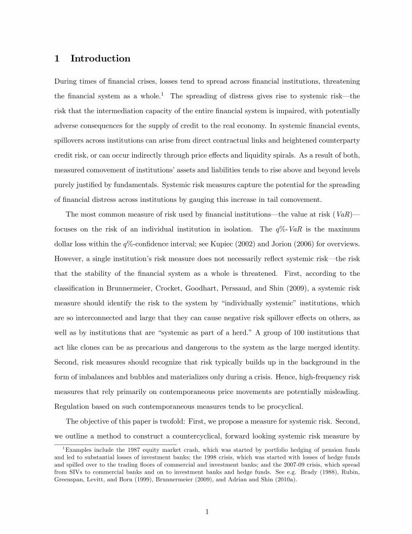
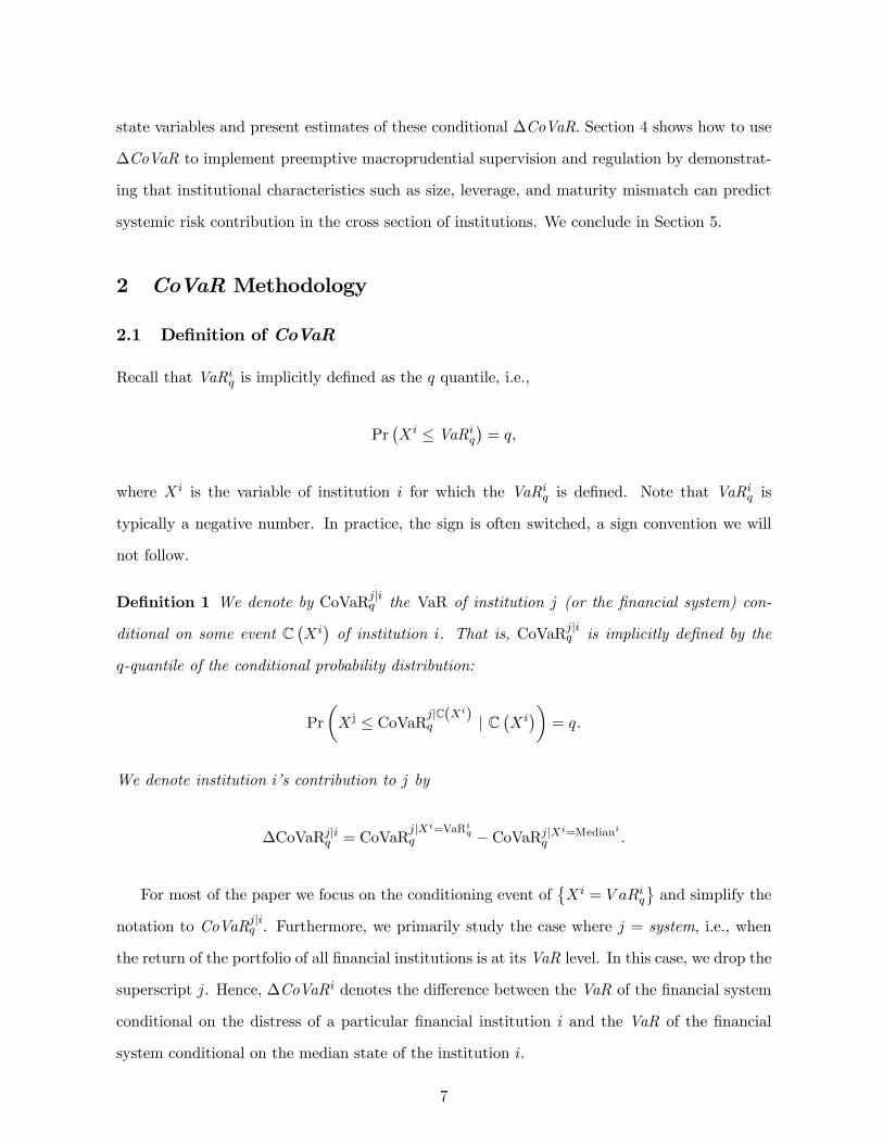
connection between an institution’s ∆CoVaR (y-axis) and its VaR (x-axis), as Figure 1 shows.
Another advantage of our co-risk measure is that it is general enough to study the risk
spillovers from institution to institution across the whole financial network. For example, ∆
CoVaR| captures the increase in risk of individual institution when institution falls into
2Just as VaR sounds like variance, CoVaR sounds like covariance. This analogy is no coincidence. In fact,
under many distributional assumptions (such as the assumption that shocks are conditionally Gaussian), the VaR
of an institution is indeed proportional to the variance of the institution, and the CoVaR of an institution is
proportional to the covariance of the financial system and the individual institution.
2
WB
WFC
JPM
BACCMER
BSC
MS
LEH
GS
AIG
MET
FNM
FRE
−6
−5
−4
−3
−2
−1
ΔCoV
aR
−12 −11 −10 −9 −8 −7Institution VaR
Commercial Banks Investment Banks
Insurance Companies GSEs
ΔCoVaR vs. VaR
Figure 1: The scatter plot shows the weak link between institutions’ risk in isolation, measured
by VaR (x-axis), and institutions’ contribution to system risk, measured by ∆CoVaR (y-axis).
The VaR and∆CoVaR are unconditional 1% measures estimated as of 2006Q4 and are reported
in weekly percent returns for merger adjusted entities. VaR is the 1% quantile of firm returns,
and ∆CoVaR gives the percentage point change in the financial system’s 1% VaR when a
particular institution realizes its own 1% VaR. The institutions used in the figure are listed in
Appendix D.
distress. To the extent that it is causal, it captures the risk spillover effects that institution
causes on institution . Of course, it can be that institution ’s distress causes a large risk
increase in institution , while institution causes almost no risk spillovers onto institution .
That is, there is no reason why ∆CoVaR| should equal ∆ CoVaR| .
So far, we have deliberately not specified how to estimate the CoVaR measure, since there are
many possible ways. In this paper, we primarily use quantile regressions, which are appealing for
their simplicity and efficient use of data. Since we want to capture all forms of risk, including not
only the risk of adverse asset price movements, but also funding liquidity risk (which is equally
important), our estimates of ∆CoVaR are based on (weekly) changes in (market-valued) total
assets of all publicly traded financial institutions. However, ∆CoVaR can also be estimated
using methods such as GARCH models, as we show in the appendix.
Our paper also addresses the problem that (empirical) risk measures suffer from the rarity of
“tail observations”. After a string of good news, risk seems tamed, but, when a new tail event
3
occurs, the estimated risk measure may sharply increase. This problem is most pronounced if
the data samples are short. Hence, regulatory requirements should be based on forward looking
risk measures. We propose the implementation of a forward-∆CoVaR that is constructed to be
forward looking and countercyclical.
We calculate unconditional and conditional measures of ∆CoVaR using the full length of
available data. We use weekly data from 1986Q1 to 2010Q4 for all publicly traded commercial
banks, broker-dealers, insurance companies, and real estate companies. While the unconditional
∆CoVaR estimates are constant over time, the conditional ones model variation of ∆CoVaR
as a function of state variables that capture the evolution of tail risk dependence over time.
These state variables include the slope of the yield curve, the aggregate credit spread, and
implied equity market volatility from VIX. We first estimate ∆CoVaR conditional on the state
variables. In a second step we use panel regressions, and relate these time-varying ∆CoVaRs–in
a predictive, Granger causal sense–to measures of each institution’s characteristics like maturity
mismatch, leverage, market-to-book, size, and market beta.
We show that the predicted values from the panel regressions (which we call “forward
∆CoVaRs”) exhibit countercyclicality. In particular, consistent with the “volatility paradox”
that low volatility environments breed the build up of systemic risk, the forward ∆CoVaRs
are strongly negatively correlated with the contemporaneous ∆CoVaRs. We also demonstrate
that the “forward-∆CoVaRs” have out of sample predictive power for realized correlation in
tail events. In particular, the forward-∆CoVaRs estimated using data through the end of 2006
predicted half of the cross sectional dispersion in realized covariance during the financial crisis
of 2008.
The forward-∆CoVaR can be used to monitor the buildup of systemic risk in a forward
looking manner. It indicates which firms are expected to contribute most to systemic financial
crisis, based on current firm characteristics. The forward-∆CoVaR can thus be used to calibrate
the systemic risk capital surcharges. A capital surcharge based on (forward) systemic risk
contribution changes ex-ante incentives to conduct activities that generate systemic risk. In
addition, it increases the capital buffer of systemically important financial institutions, thus
protecting the financial system against the risk spillovers and externalities from systemically
important financial institutions.
4
Related Literature. Our co-risk measure is motivated by theoretical research on externalities
across financial institutions that give rise to amplifying liquidity spirals and persistent distor-
tions. CoVaR tries to capture externalities, together with fundamental comovement. CoVaR
also relates to econometric work on contagion and spillover effects.
Spillovers and “externalities” can give rise to excessive risk taking and leverage in the run-up
phase. The externalities arise because each individual institution takes potential fire-sale prices
as given, while as a group they cause the fire-sale prices. In an incomplete market setting,
this pecuniary externality leads to an outcome that is not even constrained Pareto efficient.
This result was derived in a banking context in Bhattacharya and Gale (1987) and a general
equilibrium incomplete market setting by Stiglitz (1982) and Geanakoplos and Polemarchakis
(1986). Prices can also affect borrowing constraints. These externality effects are studied in
within an international finance context by Caballero and Krishnamurthy (2004), and most re-
cently shown in Lorenzoni (2008), Acharya (2009), Stein (2009), and Korinek (2010). Runs on
financial institutions are dynamic co-opetition games and lead to externalities, as does banks’
liquidity hoarding. While hoarding might be microprudent from a single bank’s perspective it
need not be macroprudent (fallacy of the commons). Finally, network effects can also lead to
externalities, as emphasized by Allen, Babus, and Carletti (2010).
Procyclicality occurs because risk measures tend to be low in booms and high in crises.
The margin/haircut spiral and precautionary hoarding behavior outlined in Brunnermeier and
Pedersen (2009) and Brunnermeier and Sannikov (2009) led financial institutions to shed assets
at fire-sale prices. Adrian and Shin (2010b) and Gorton and Metrick (2010) provide empirical
evidence for the margin/haircut spiral. Borio (2004) is an early contribution that discusses a
policy framework to address margin/haircut spirals and procyclicality.
Recently a number of systemic risk measures complementary to CoVaR have recently been
proposed. Huang, Zhou, and Zhu (2010) develop a systemic risk indicator measured by the
price of insurance against systemic financial distress, based on credit default swap (CDS) prices.
Acharya, Pedersen, Philippon, and Richardson (2010) focus on high-frequency marginal expected
shortfall as a systemic risk measure. Like our “exposure CoVaR”, they switch the conditioning
and addresses the question which institutions are most exposed to a financial crisis as opposed
to which institution contributes most to a crisis. Importantly, their analysis focuses on the cross
5
sectional comparison across financial institutions and do not address the problem of procyclical-
ity that arises from contemporaneuous risk measurement. In other words, they do not address
the stylized fact that risk is building up in the background during boom phases characterized by
low volatility and materializes only in crisis times. Billio, Getmansky, Lo, and Pelizzon (2010)
propose a systemic risk measure that relies on Granger causality among firms. Giglio (2011)
uses a nonparametric approach to derive bounds of systemic risk from CDS prices. A number of
recent papers have extended the CoVaR method and applied it to additional financial sectors.
For example, Adams, Füss, and Gropp (2010) study risk spillovers among financial institutions,
using quantile regressions; Wong and Fong (2010) estimate CoVaR for the CDS of Asia-Pacific
banks; Gauthier, Lehar, and Souissi (2009) estimate systemic risk exposures for the Canadian
banking system.
The CoVaR measure is related to the literature on volatility models and tail risk. In a seminal
contribution, Engle and Manganelli (2004) develop CAViaR, which uses quantile regressions in
combination with a GARCH model to model the time varying tail behavior of asset returns.
Manganelli, Kim, and White (2011) study a multivariate extension of CAViaR, which can be
used to generate a dynamic version of the CoVaR systemic risk measure.
The CoVaR measure can also be related to an earlier literature on contagion and volatility
spillovers (see Claessens and Forbes (2001) for an overview). The most common method to test
for volatility spillover is to estimate multivariate GARCH processes. Another approach is to
use multivariate extreme value theory. Hartmann, Straetmans, and de Vries (2004) develop a
contagion measure that focuses on extreme events. Danielsson and de Vries (2000) argue that
extreme value theory works well only for very low quantiles.
Another important strand of the literature, initiated by Lehar (2005) and Gray, Merton, and
Bodie (2007), uses contingent claims analysis to measure systemic risk. Bodie, Gray, and Merton
(2007) develop a policy framework based on the contingent claims. Segoviano and Goodhart
(2009) use a related approach to measure risk in the banking system.
Outline. The remainder of the paper is organized in four sections. In Section 2, we outline
the methodology and define ∆CoVaR and its properties. In Section 3, we outline the estima-
tion method via quantile regressions. We also introduce time-varying ∆CoVaR conditional on
6
state variables and present estimates of these conditional ∆CoVaR. Section 4 shows how to use
∆CoVaR to implement preemptive macroprudential supervision and regulation by demonstrat-
ing that institutional characteristics such as size, leverage, and maturity mismatch can predict
systemic risk contribution in the cross section of institutions. We conclude in Section 5.
2 CoVaR Methodology
2.1 Definition of CoVaR
Recall that VaR is implicitly defined as the quantile, i.e.,
Pr¡ ≤ VaR
¢= ,
where is the variable of institution for which the VaR is defined. Note that VaR
is
typically a negative number. In practice, the sign is often switched, a sign convention we will
not follow.
Definition 1 We denote by CoVaR| the VaR of institution (or the financial system) con-
ditional on some event C¡¢of institution . That is, CoVaR
| is implicitly defined by the
-quantile of the conditional probability distribution:
notation to CoVaR| . Furthermore, we primarily study the case where = system, i.e., when
the return of the portfolio of all financial institutions is at its VaR level. In this case, we drop the
superscript . Hence, ∆CoVaR denotes the difference between the VaR of the financial system
conditional on the distress of a particular financial institution and the VaR of the financial
system conditional on the median state of the institution .
7
The more general definition of CoVaR|–i.e., the VaR of institution conditional on in-
stitution being at its VaR level–allows the study of spillover effects across a whole financial
network. Moreover, we can derive CoVaR| which answers the question of which insti-
tutions are most at risk should a financial crisis occur. ∆CoVaR| reports institution ’s
increase in value-at-risk in the case of a financial crisis. We call ∆CoVaR| the “expo-
sure CoVaR,” because it measures the extent to which an individual institution is affected by
systemic financial events.3
2.2 The Economics of Systemic Risk
Systemic risk has two important components. First, it builds up in the background during credit
booms when contemporaneously measured risk is low. This buildup of systemic risk during times
of low measured risk gives rise to a “volatility paradox.” The second component of systemic risk
relates to the spillover effects that amplify initial adverse shocks in times of crisis.
The contemporaneous ∆CoVaR measure quantifies these spillover effects by measuring how
much an institution adds to the overall risk of the financial system. The spillover effects can
be direct, through contractual links among financial institutions. This is especially the case
for institutions that are “too interconnected to fail.” Indirect spillover effects are quantitatively
more important. Selling off assets can lead to mark-to-market losses for all market participants
who hold a similar exposure–common exposure effect. Moreover, the increase in volatility
might tighten margins and haircuts forcing other market participants to delever as well (margin
spiral). This can lead to crowded trades which increases the price impact even further.
The notion of systemic risk that we are using in this paper captures direct and indirect
spillover effects and is based on the tail covariation between financial institutions and the fi-
nancial system. Definition 1 implies that financial institutions whose distress coincides with the
distress of the financial system will have a high systemic risk measure. Systemic risk contribu-
tion gauges the extent to which financial system stress increases conditional on the distress of
a particular firm, and thus captures spillover effects. It should be noted, however, that the ap-
proach taken in this paper is a statistical one, without explicit reference to structural economic
3Huang, Zhou, and Zhu (2010) and Acharya, Pedersen, Philippon, and Richardson (2010) propose systemic
risk measures that reverse the conditioning of CoVaR. These alternative measures thus use the same conditioning
logic as that for the “exposure CoVaR”.
8
models. Nevertheless, we conjecture that the ∆CoVaR measure would give rise to meaningful
time series and cross sectional measurement of systemic risk in such economic theories.
Many of these spillovers are externalities. That is, when taking on the initial position
with low market liquidity funded with short-term liabilities–i.e. with high liquidity mismatch,
each individual market participant does not internalize that his subsequent individually optimal
response in times of crisis will cause a (pecuniary) externality on others. As a consequence the
initial risk taking is often excessive in the run-up phase.
In section 4, we construct a “forward ∆CoVaR”. This forward measure captures the stylized
fact that systemic risk is building up in the background, especially during in low volatility
environments. As a result, contemporaneous systemic risk measures are not suited to fully
capture the buildup component of systemic risk. Our “forward ∆CoVaR” measure avoids the
“procyclicality pitfall” by estimating the relationship between current firm characteristics and
future spillover effects, as proxied by ∆CoVaR.
2.3 Properties of CoVaR
Cloning Property. Our CoVaR definition satisfies the desired property that, after splitting
one large “individually systemic” institution into smaller clones, the CoVaR of the large
institution (in return space) is exactly the same as the CoVaRs of the clones. Put differently,
conditioning on the distress of a large systemic institution is the same as conditioning on one of
the clones.
Causality. Note that the ∆CoVaR measure does not distinguish whether the contribution
is causal or simply driven by a common factor. We view this as a virtue rather than as a
disadvantage. To see this, suppose a large number of small hedge funds hold similar positions
and are funded in a similar way. That is, they are exposed to the same factors. Now, if only one
of the small hedge funds falls into distress, this will not necessarily cause any systemic crisis.
However, if the distress is due to a common factor, then the other hedge funds–all of which
are “systemic as part of a herd”–will likely be in distress. Hence, each individual hedge fund’s
co-risk measure should capture the notion of being “systemic as part of a herd” even in the
absence of a direct causal link. The ∆CoVaR measure achieves exactly that. Moreover, when
9
we estimate ∆CoVaR, we control for lagged state variables that capture variation in tail risk
not directly related to the financial system risk exposure.
Tail Distribution. CoVaR focuses on the tail distribution and is more extreme than the
unconditional VaR, as CoVaR is a VaR that conditions on a “bad event”–a conditioning that
typically shifts the mean downwards, increases the variance, and potentially increases higher
moments such as negative skewness and kurtosis. The CoVaR, unlike the covariance, reflects
shifts in all of these moments. Estimates of CoVaR for different allow an assessment of the
degree of systemic risk contribution for different degrees of tailness.
Conditioning. Note that CoVaR conditions on the event C, which we mostly assume to be
the event that institution is at its VaR level, occurs with probability . That is, the likelihood
of the conditioning event is independent of the riskiness of ’s strategy. If we were to condition
on a return level of institution (instead of a quantile), then more conservative (i.e., less risky)
institutions could have a higher CoVaR simply because the conditioning event would be a more
extreme event for less risky institutions.
Endogeneity of Systemic Risk. Note that each institution’s CoVaR is endogenous and
depends on other institutions’ risk taking. Hence, imposing a regulatory framework that inter-
nalizes externalities alters the CoVaR measures. We view as a strength the fact that CoVaR is
an equilibrium measure, since it adapts to changing environments and provides an incentive for
each institution to reduce its exposure to risk if other institutions load excessively on it.
Directionality. CoVaR is directional. That is, the CoVaR of the system conditional on
institution does not equal the CoVaR of institution conditional on the system.
Exposure CoVaR. The direction of conditioning that we consider is ∆CoVaR| . How-
ever, for risk management questions, it is sometimes useful to compute the opposite conditioning,
∆CoVaR| , which we label exposure “Exposure CoVaR”. The Exposure CoVaR is a mea-
sure of an individual institution’s exposure to system wide distress, and is similar to the stress
tests performed by individual institutions.
10
CoES. Another attractive feature of CoVaR is that it can be easily adopted for other “corisk-
measures.” One of them is the co-expected shortfall, Co-ES. Expected shortfall has a number
of advantages relative to VaR4 and can be calculated as a sum of VaRs. We denote the CoES,
the expected shortfall of the financial system conditional on ≤ VaR of institution . That is,
CoES is defined by the expectation over the -tail of the conditional probability distribution:
£system |system ≤ CoVaR
¤Institution ’s contribution to CoES is simply denoted by
∆CoES = £system |system ≤ CoVaR
¤−£system |system ≤ CoVaR
50%
¤.
Ideally, one would like to have a co-risk measure that satisfies a set of axioms as, for example,
the Shapley value does (recall that the Shapley value measures the marginal contribution of a
player to a grand coalition).5
2.4 Market-Valued Total Financial Assets
Our analysis focuses on the VaR and ∆CoVaR
of growth rates of market-valued total financial
assets. More formally, denote by the market value of an intermediary ’s total equity, and
by the ratio of total assets to book equity. We define the growth rate of market valued
total assets, , by
=
·
−−1 ·
−1
−1 · −1
= −
−1−1
, (1)
where =
· . Note that
=
· =
·¡
¢, where
are book-valued total assets of institution . We thus apply the market-to-book equity ratio to
transform book-valued total assets into market-valued total assets.6
4Note that the VaR is not subadditive and does not take distributional aspects within the tail into account.
These concerns are however more of theoretical nature since the exact distribution within the tails is difficult to
estimate.5Tarashev, Borio, and Tsatsaronis (2009) elaborate the Shapley value further, and Cao (2010) shows how to
use Shapley values to calculate systemic risk contributions of CoVaR. See also Brunnermeier and Cheridito (2011).6There are several alternatives to generating market valued total assets. One possibility is to use a structural
model of firm value in order to calculate market valued assets. Another possibility is to add the market value of
equity to the book value of debt. We did not find that any of these alternative ways to generate market valued
total assets had a substantial impact on the qualitative outcomes of the subsequent analysis.
11
Our analysis uses publicly available data. In principle, a systemic risk supervisor could
compute the VaR and ∆CoVaR
from a broader definition of total assets which would include
off-balance-sheet items, exposures from derivative contracts, and other claims that are not prop-
erly captured by the accounting value of total assets. A more complete description of the assets
and exposures of institutions would potentially improve the measurement of systemic risk and
systemic risk contribution. Conceptually, it is straightforward to extend the analysis to such a
broader definition of total assets.
We focus on the VaR and ∆CoVaR
of total assets as they are most closely related to the
supply of credit to the real economy. Ultimately, systemic risk is of concern for economic welfare
as systemic financial crisis have the potential to inefficiently lower the supply of credit to the
nonfinancial sector.
Our analysis of the VaR and ∆CoVaR
for market valued assets could be extended to
compute the risk measures for equities or liabilities. For example, the ∆CoVaR for liabilities
captures the extent to which financial institutions rely on debt funding–such as repos or com-
mercial paper–that can collapse during systemic risk events. Equity is the residual between
assets and liabilities, so the ∆CoVaR measure applied to equity can give additional information
about the systemic risk embedded in the asset-liability mismatch. The study of the properties of
∆CoVaR for these other items of intermediary balance sheets is a potentially promising avenue
for future research.
2.5 Financial Institution Data
We focus on publicly traded financial institutions, consisting of four financial sectors: commercial
banks, security broker-dealers (including the investment banks), insurance companies, and real
estate companies. We start our sample in 1986Q1 and end it in 2010Q4. The data thus cover
three recessions (1991, 2001, and 2007-09) and several financial crisis (1987, 1998, 2000, and
2008). We obtain daily market equity data from CRSP and quarterly balance sheet data from
COMPUSTAT. We have a total of 1226 institutions in our sample. For bank holding companies,
we use additional asset and liability variables from the FR Y9-C reports. Appendix C provides
a detailed description of the data.
12
3 CoVaR Estimation
In this section we outline CoVaR estimation. In Section 3.1, we describe the basic time-invariant
regressions that are used to generate Figure 1. In Section 3.2, we describe estimation of the
time-varying, conditional CoVaR. Details on the econometrics are given in Appendix A. Section
3.3 provides estimates of CoVaR and discusses properties of the estimates.
3.1 Estimation Method: Quantile Regression
We use quantile regressions to estimate CoVaR.7 To see the attractiveness of quantile regres-
sions, consider the predicted value of a quantile regression of the financial sector on a
particular institution or portfolio for the -quantile:
= +
, (2)
where denotes the predicted value for a particular quantile conditional on institution
.8 In principle, this regression could be extended to allow for nonlinearities by introducing
higher order dependence of the system return as a function of returns to institution . From the
definition of value at risk, it follows directly that
VaR | =
. (3)
That is, the predicted value from the quantile regression of the system on institution gives
the value at risk of the financial system conditional on , since the VaR given is just the
conditional quantile. Using a particular predicted value of =VaR yields our CoVaR
7The CoVaR measure can be computed in various ways. Quantile regressions are a particularly efficient way
to estimate CoVaR. It should be emphasized, however, that quantile regressions are by no means the only way
to estimate CoVaR. Alternatively, CoVaR can be computed from models with time-varying second moments,
from measures of extreme events, or by bootstrapping past returns. In Appendix B we provide a comparison to
estimation using a bivariate GARCH model.8Note that a median regression is the special case of a quantile regression where = 50%.We provide a short
synopsis of quantile regressions in the context of linear factor models in Appendix A. Koenker (2005) provides a
more detailed overview of many econometric issues.
While quantile regressions are used regularly in many applied fields of economics, their applications to financial
economics are limited.
13
framework, our specific CoVaR measure is simply given by
CoVaR|=VaR := VaR
|VaR = +
VaR. (4)
The ∆CoVaR is then given by
∆CoVaR| =
¡VaR
−VaR50%
¢ (5)
The unconditional VaR and ∆CoVaR
estimates for Figure 1 are based on equation (5), where
an asset’s estimated VaR is simply the
-quantile of its returns. In the remainder of the
paper, we use conditional VaR and ∆CoVaR estimates that explicitly model the time variation
of the joint distribution of asset returns as a function of lagged systematic state variables.
3.2 Time Variation Associated With Systematic State Variables
The previous section presented a methodology for estimating CoVaR that is constant over time.
To capture time variation in the joint distribution of and, we estimate the conditional
distribution as a function of state variables. We indicate time-varying CoVaR and VaR with
a subscript and estimate the time variation conditional on a vector of lagged state variables
−1. We run the following quantile regressions in the weekly data (where is an institution):
= + −1 + , (6a)
= | + |
+ |−1 + | . (6b)
We then generate the predicted values from these regressions to obtain
() = + −1, (7a)
() = | +
|
() + |−1. (7b)
14
Finally, we compute ∆ for each institution:
∆ () =
()− (50%) (8)
= | ¡
()−
(50%)¢. (9)
From these regressions, we obtain a panel of weekly ∆CoVaR. For the forecasting regressions
in Section 4, we generate a quarterly time series by summing the risk measures within each
quarter.
The systematic state variables−1 are lagged. They should not be interpreted as systematic
risk factors, but rather as conditioning variables that are shifting the conditional mean and the
conditional volatility of the risk measures. Note that different firms can load on these risk
factors in different directions, so that particular correlations of the risk measures across firms–
or correlations of the different risk measures for the same firm–are not imposed by construction.
State variables: To estimate the time-varying CoVaR and VaR, we include a set of state
variables that are (i) well known to capture time variation in conditional moments of asset
returns, and (ii) liquid and easily tradable. We restrict ourselves to a small set of risk factors to
avoid overfitting the data. Our factors are:
(i) VIX, which captures the implied volatility in the stock market reported by the Chicago
Board Options Exchange.9
(ii) A short term “liquidity spread,” defined as the difference between the three-month repo
rate and the three-month bill rate. This liquidity spread measures short-term liquidity risk. We
use the three-month general collateral repo rate that is available on Bloomberg, and obtain the
three-month Treasury rate from the Federal Reserve Bank of New York.10
(iii) The change in the three-month Treasury bill rate from the Federal Reserve Board’s
H.15. We use the change in the three-month Treasury bill rate because we find that the change,
9The VIX is available only since 1990. We use the VXO for the 1986-90 period by running a regression of
the VIX on the VXO for the 1990-2010 period and then using the predicted value from that regression for the
1986-89 period.10The three-month repo rate is available on Bloomberg only since 1990. We use the three-month Libor rate as
reported by the British Bankers Association for the 1986-90 period by running a regression of the repo rate on
the libor rate for the 1990-2010 period and then using the predicted value from that regression for the 1986-89
period.
15
not the level, is most significant in explaining the tails of financial sector market-valued asset
returns.
In addition, we consider the following two fixed-income factors that capture the time variation
in the tails of asset returns:
(iv) The change in the slope of the yield curve, measured by the yield spread between the
ten-year Treasury rate and the three-month bill rate obtained from the Federal Reserve Board’s
H.15 release.
(v) The change in the credit spread between BAA-rated bonds and the Treasury rate (with
the same maturity of ten years) from the Federal Reserve Board’s H.15 release.
We further control for the following equity market returns:
(vi) The weekly equity market return from CRSP.
(vii) The weekly real estate sector return in excess of the market return (from the real estate
companies with SIC code 65-66).
The following table give summary statistics for the state variables. We also report the 1%
stress level, which is the variable’s mean conditional on the financial system being in its historical
1% tail.
[Table 1 here]
Table 1 provides summary statistics of the state variables. The 1% stress level is the level
of each respective variable during the 1% worst weeks for financial system asset returns. For
example, the average of the VIX during the stress periods is 51.66, as the worst times for
the financial system include the times when the VIX was highest. Similarly, the stress level
corresponds to a high level of the liquidity spread, a sharp decline in the Treasury bill rate,
sharp increases of the term and credit spreads, and large negative equity return realizations.
In general, by comparing the extreme values of the state variables to the numbers of standard
deviations away from their mean, we can see that the distributions appear highly skewed.
3.3 CoVaR Summary Statistics
Table 2 provides the estimates of our weekly conditional 1%-CoVaR measures that we obtain
from using quantile regressions. Each of the summary statistics constitutes the universe of
16
financial institutions.
[Table 2 here]
Line (1) of Table 2 give the summary statistics for the market-valued total asset growth
rates; line (2) gives the summary statistics for the VaR for each institution; line (3) gives the
summary statistics for ∆CoVaR; lines (4) gives the summary statistics for the 1%-stress level
of ∆CoVaR; and line (5) gives the summary statistics for the financial system value at risk,
VaR . The stress ∆CoVaR
is estimated by substituting the worst 1% of state variable
realizations into the ∆CoVaR estimates.
Recall that ∆CoVaR measures the marginal contribution of institution to overall systemic
risk and reflects the difference between the value at risk of the financial universe conditional
on the stressed and the median state of institution . We report the mean, standard deviation,
and number of observations for each of the items in Table 2. All of the numbers are expressed
in weekly percent returns. We have a total of 1226 institutions in the sample, with an average
length of 645 weeks. The institution with the longest history spans all 1300 weeks of the 1986Q1-
2010Q4 sample period. We require institutions to have at least 260 weeks of asset return data
in order to be included in the panel. In the following analysis, we focus primarily on the 1%
and the 5% quantiles, corresponding to the worst 13 weeks and the worst 65 weeks over the
sample horizon, respectively. It is straightforward to estimate more extreme tails following the
methodology laid forward by Chernozhukov and Du (2008), an analysis that we leave for future
research. In the following analysis, we find results that are largely qualitatively similar for the
1% and the 5% quantiles.
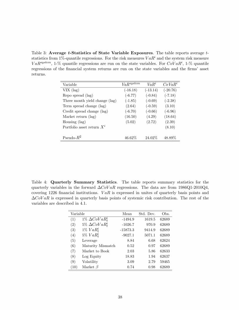
[Table 3 here]
We obtain time variation of the risk measures by running quantile regressions of asset returns
on the lagged state variables. We report average −stats of these regressions in Table 3. A higherVIX, higher repo spread, and lower market return tend to be associated with more negative
risk measures. In addition, increases in the three-month yield, declines in the term spread,
and increases the credit spread tend to be associated with larger risk. Overall, the average
significance of the conditioning variables reported in Table 3 show that the state variables do
indeed proxy for the time variation in the quantiles and particularly in CoVaR.
17
3.4 CoVaR versus VaR
Figure 1 shows that, across institutions, there is only a very loose link between an institution’s
VaR and its contribution to systemic risk as measured by ∆CoVaR. Hence, imposing financial
regulation solely based on the risk of an institution in isolation might not be sufficient to insulate
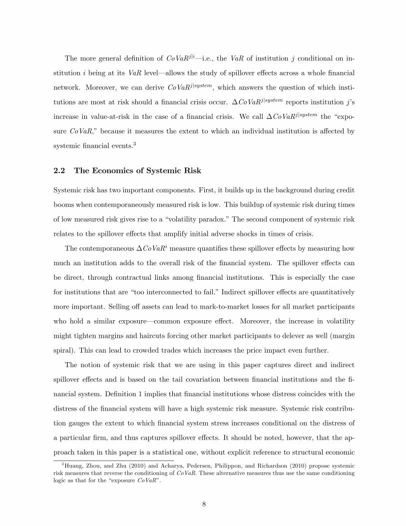
the financial sector against systemic risk. Figure 2 repeats the scatter plot of ∆CoVaR against
VaR for 240 portfolios, grouped by 60 portfolios for each of the four financial industries.11 We
do so, since one might argue that firms change their risk taking behavior over the sample span
of 1986 to 2010. Using portfolios, ∆CoVaR and VaR have only a weak relationship in the
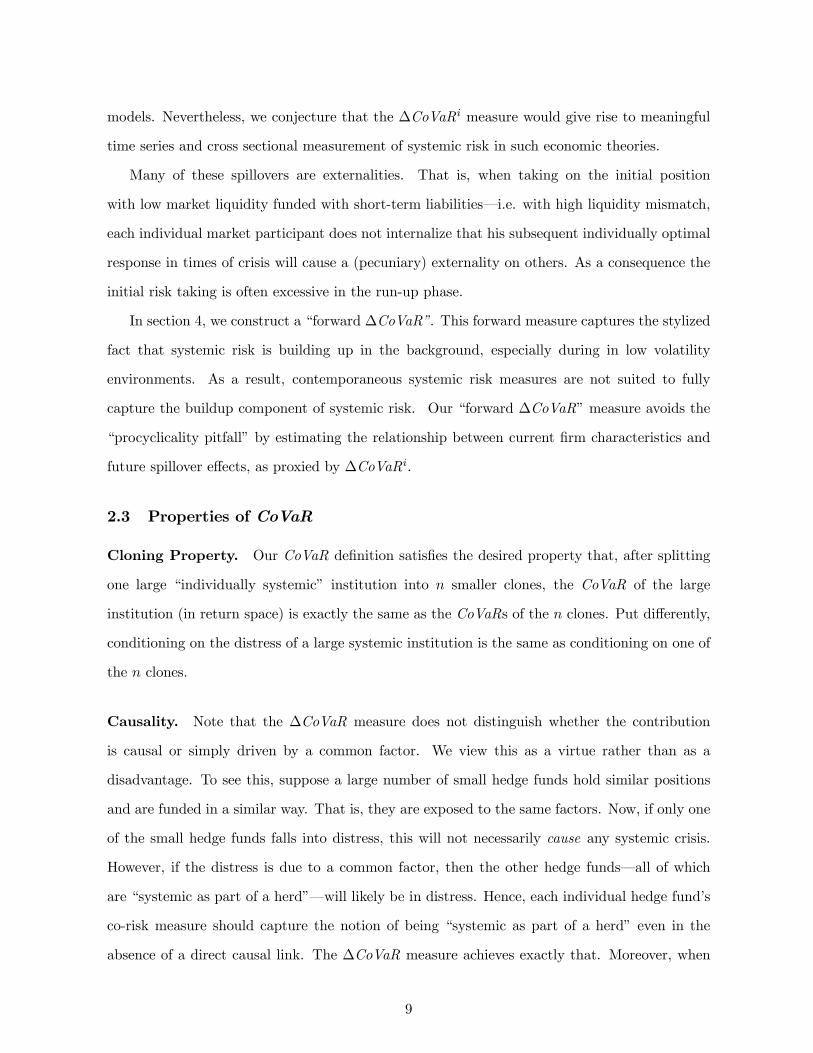
cross section. However, they have a strong relationship in the time series. This can be seen in
Figure 3, which plots the time series of the ∆CoVaR and VaR for the portfolio of large broker
dealers over time. We note that the cross sectional average of ∆CoVaR including all institutions
has a very close time series relationship with the value at risk of the financial system, VaR,
per construction. One way to interpret the ∆CoVaR is by viewing them as cross sectional
allocation of system wide risk to the various institutions.
4 Forward-∆CoVaR
In this section, we calculate forward looking systemic risk measures that can be used for financial
stability monitoring, and as a basis for (countercyclical) macroprudential policy. We first present
the construction of the “forward -∆CoVaR”, and then present out of sample tests. We finally
discuss how the measures could be used as a basis for capital surcharge calibrations.
Instead of tying financial regulation directly to ∆CoVaR, we propose to link it to financial
institutions’ characteristics that predict their future ∆CoVaR. This addresses two key issues
of systemic risk regulation: measurement accuracy and procyclicality. Any tail risk measure,
estimated at a high frequency, is by its very nature imprecise. Quantifying the relationship
between∆CoVaR and more easily observable institution-specific variables, such as size, leverage,
and maturity mismatch, allows for more robust inference than measuring ∆CoVaR directly.
Furthermore, using these variables to predict future contributions to systemic risk addresses
the inherent procyclicality of market-based risk measures. This ensures that ∆CoVaR-based
11The portfolios are constructed from quintiles by market-valued assets, 2- year market-valued asset growth,
maturity mismatch, equity volatility, leverage, and market-to-book ratio for each of the four industries.
18
−6
−4
−2
0ΔC
oVaR
−12 −10 −8 −6 −4Portfolio VaR
Commercial Banks
−6
−4
−2
0ΔC
oVaR
−12 −10 −8 −6 −4Portfolio VaR
Insurance Companies
−2.
5−
2−
1.5
−1
−.5
0ΔC
oVaR
−25 −20 −15 −10 −5Portfolio VaR
Real Estate
−5
−4
−3
−2
−1
0ΔC
oVaR
−16 −14 −12 −10 −8Portfolio VaR
Broker Dealers
Time Series Average − ΔCoVaR vs. VaR
Figure 2: The scatter plot shows the weak cross-sectional link between the time-series average
of a portfolio’s risk in isolation, measured by VaR (x-axis), and the time-series average of a
portfolio’s contribution to system risk, measured by∆CoVaR (y-axis). The VaR and∆CoVaR
are in units of weekly percent returns to total market-valued financial assets and measured at
the 1% level.
financial regulation is implemented in a forward-looking way that counteracts the procyclicality
of current regulation.
4.1 Constructing the Forward-∆CoVaR
We relate estimates of time-varying ∆CoVaR to characteristics of financial institutions. We
collect the following set of characteristics:
1. leverage, defined as total assets / total equity (in book values);
2. maturity mismatch, defined as (short term debt - cash) / total liabilities ;
3. market-to-book, defined as the ratio of the market to the book value of total equity;
4. size, defined by the log of total book equity;
5. equity return volatility, computed from daily equity return data within each quarter;
6. equity market beta calculated from daily equity return data within each quarter.
[Table 4 here]
[Table 5 here]
19
-30
-20
-10
010
2030
(Str
ess)
C
oVaR
-60
-40
-20
020
40A
sset
Gro
wth
, VaR
1985 1990 1995 2000 2005 2010
Asset Growth VaR
CoVaR Stress CoVaR
Large Broker Dealers
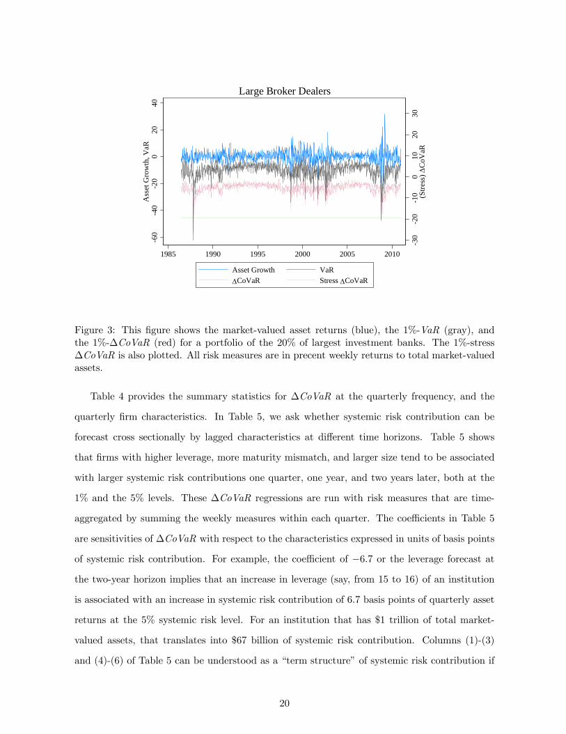
Figure 3: This figure shows the market-valued asset returns (blue), the 1%-VaR (gray), and
the 1%-∆CoVaR (red) for a portfolio of the 20% of largest investment banks. The 1%-stress
∆CoVaR is also plotted. All risk measures are in precent weekly returns to total market-valued
assets.
Table 4 provides the summary statistics for ∆CoVaR at the quarterly frequency, and the
quarterly firm characteristics. In Table 5, we ask whether systemic risk contribution can be
forecast cross sectionally by lagged characteristics at different time horizons. Table 5 shows
that firms with higher leverage, more maturity mismatch, and larger size tend to be associated
with larger systemic risk contributions one quarter, one year, and two years later, both at the
1% and the 5% levels. These ∆CoVaR regressions are run with risk measures that are time-
aggregated by summing the weekly measures within each quarter. The coefficients in Table 5
are sensitivities of ∆CoVaR with respect to the characteristics expressed in units of basis points
of systemic risk contribution. For example, the coefficient of −67 or the leverage forecast atthe two-year horizon implies that an increase in leverage (say, from 15 to 16) of an institution
is associated with an increase in systemic risk contribution of 67 basis points of quarterly asset
returns at the 5% systemic risk level. For an institution that has $1 trillion of total market-
valued assets, that translates into $67 billion of systemic risk contribution. Columns (1)-(3)
and (4)-(6) of Table 5 can be understood as a “term structure” of systemic risk contribution if
20
read from right to left. The comparison of Panels A and B provide a gauge of the “tailness” of
systemic risk contribution.
The regression coefficients of Table 5 can be used to weigh the relative importance of various
firm characteristics. To make this more explicit, consider the following example: Suppose a small
bank is subject to a tier-one capital requirement of 7%. That is, the “leverage ratio” cannot
exceed 1 : 14.12 Our analysis answers the question of how much stricter the capital requirement
should be for a larger bank with the same leverage, assuming that the small bank and the large
bank are allowed a fixed level of systemic risk contribution ∆CoVaR. If the larger bank is 10
percent larger than the smaller bank, then the size coefficient predicts that its ∆CoVaR per
unit of capital is 27 basis points larger than the small bank’s ∆CoVaR. To ensure that both
banks have the same ∆ CoVaR per unit of capital, the large bank would have to reduce its
maximum leverage from 1 : 14 to 1 : 10. In other words, the large bank should face a capital
requirement of 10% instead of 7%. The exact trade-off between size and leverage is given by
the ratio of the two respective coefficients of our forecasting regressions. Of course, in order to
achieve a given level of systemic risk contribution per units of total assets, instead of lowering
the size, the bank could also reduce its maturity mismatch or improve its systemic risk profile
along other dimensions. Similarly, for a Pigouvian taxation scheme, the regression coefficients
should determine the weight of leverage, maturity mismatch, size, and other characteristics in
forming the tax base.
This methods allows the connection of macroprudential policy with frequently and robustly
measured characteristics. ∆CoVaR–like any tail risk measure–relies on relatively few extreme-
crisis data points. Hence, adverse movements, especially followed by periods of stability, can
lead to sizable increases in tail risk measures. In contrast, measurement of characteristics such
as size are very robust, and they can be measured more reliaiably at higher frequencies. The
debate on “too big to fail” suggests that size is the all-dominating variable, indicating that
large institutions should face a more stringent regulation compared to smaller institutions. As
mentioned above, unlike a co-risk measure, the “size only” approach fails to acknowledge that
many small institutions can be “systemic as part of a herd.” Our solution to this problem is to
12We are loose here, since the Basel capital requirement refers to ratio between equity capital and risk weighted
assets, while our study simply takes total assets.
21
combine the virtues of both types of measures by projecting the spillover risk measure ∆CoVaR
on multiple, more frequently observable variables.
This method can also address the procyclicality of contemporaneous risk measures. Sys-
temic risk builds up before an actual financial crisis occurs and any regulation that relies on
contemporaneous risk measure estimates would be unnecessarily tight after adverse events and
unnecessarily loose in periods of stability. In other words, it would amplify the adverse impacts
after bad shocks, while also amplifying balance sheet expansions in expansions.13 Hence, we
propose to focus on variables that can be reliably measured at a quarterly frequency and predict
future, rather than contemporaneous, ∆CoVaR.
4.2 Forward-∆CoVaR for Bank Holding Companies
Ideally, one would like to link macroprudential policies to more instititutional characteristics
than simply size, leverage, maturity mismatch etc. If one restricts the sample to bank holding
companies, we have more characteristic data to extend our method. On the asset side of banks’
balance sheets, we use loans, loan-loss allowances, intangible loss allowances, intangible assets,
and trading assets. Each of these asset composition variables is expressed as a percent of total
book assets. The cross-sectional regressions with these asset composition variables are reported
in Panel A of Table 6. In order to capture the liability side of banks’ balance sheets, we use
interest-bearing core deposits (IBC), non-interest-bearing deposits (NIB), large time deposits
(LT), and demand deposits. Each of these variables is expressed as a percent of total book
assets. The variables can be interpreted as refinements of the maturity mismatch variable used
earlier. The cross-sectional regressions with the liability aggregates are reported in Panel B of
Table 6.
[Table 6 here]
Panel A of Table 6 shows which types of liability variables are significantly increasing or
decreasing systemic risk contribution. Bank holding companies with a higher fraction of non-
interest-bearing deposits have a significantly higher systemic risk contribution, while interest
bearing core deposits and large time deposits are decreasing the forward estimate of ∆CoVaR.
13See Estrella (2004), Kashyap and Stein (2004), and Gordy and Howells (2006) for studies of the procyclical
nature of capital regulation.
22
Non-interest-bearing deposits are typically held by nonfinancial corporations and households,
and can be quickly reallocated across banks conditional on stress in a particular institution.
Interest-bearing core deposits and large time deposits, on the other hand, are more stable sources
of funding and are thus decreasing the systemic tail risk contribution (i.e., they have a posi-
tive sign). The share of deposits is not significant. The maturity-mismatch variable that we
constructed for the universe of financial institutions is no longer significant once we include the
more refined liability measures for the bank holding companies. In fact, in some specifications,
the maturity mismatch variable is significant with the wrong sign.
Panel B of Table 6 shows that loan-loss allowances and trading assets are particularly good
predictors for the cross-sectional dispersion of future systemic risk contribution. The fraction of
intangible assets is marginally significant. Conditional on these variables, the size of total loans
as a fraction of book equity tends to decrease systemic risk contribution, which might be due
to the accounting treatment of loans: loans are held at historical book value, and deteriorating
loan quality is captured by the loan-loss reserves. By including loan-loss reserves, trading assets,
and intangible assets in the regression gives rise to lower estimates of systemic risk contribution.
In summary, the results of Table 6, in comparison to Table 5, show that more informa-
tion about the balance sheet characteristics of financial institutions can potentially improve
the estimated forward ∆CoVaR. We expect additional data that capture particular activities
of financial institutions, as well as supervisory data, to lead to further improvements in the
estimation precision of forward systemic risk contribution.
4.3 Out of Sample Forward-∆CoVaR
We compute “forward ∆CoVaR”as the predicted value from the panel regression reported in
Table 5. We generate this forward ∆CoVaR “in sample” through 2000, and then out of sample
by re-estimating the panel regression each quarter, and computing the predicted value. Since
one cannot use time effects in an out of sample exercise, we use the macro state variables to
capture common variation across time.
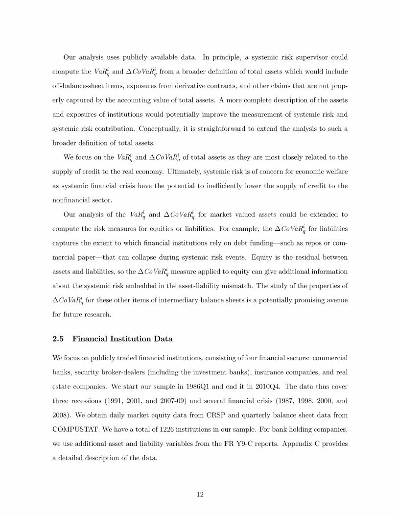
We plot the ∆CoVaR together with the two-year forward ∆CoVaR for the average of the
largest 50 financial institutions in Figure 4. The figure clearly shows the strong negative corre-
lation of the contemporaneous ∆CoVaR and the forward ∆ CoVaR. In particular, during the
23
-60
-40
-20
0C
onte
mpo
rane
ous
-24
-22
-20
-18
-16
2-ye
ar F
orw
ard
1985 1990 1995 2000 2005 2010
2-year Forward Contemporaneous
Countercyclicality
Figure 4: Out-of-Sample Forward ∆CoVaR: This figure shows average forward and contem-
poraneous 5% ∆CoVaR estimated out-of-sample for the top 50 financial institutions estimated
out-of-sample. First, weekly contemporaneous ∆ is estimated out-of-sample starting in
2000Q1 at one quarter increments with an expanding window. Forward ∆ is generated
as described in the paper but in an out-of-sample fashion, again beginning in 2000Q1. The
forward ∆ at a given date uses the data available at that time to predict ∆ two
years in the future.
credit boom of 2003-06, the contemporaneous ∆CoVaR is estimated to be small (in absolute
value), while the forward ∆CoVaR is large (in absolute value). Macroprudential regulation
based on the forward ∆CoVaR are thus countercyclical.
Next, we extend the in sample panel estimates reported in Tables 5 and 6 to out of sample
estimates. In particular, we show that the forward∆CoVaR predicts the cross section of systemic
risk realizations out of sample. In order to show the out of sample performance, we need a
measure of realized systemic risk contribution. As a proxy, we compute covariances of financial
institutions with the financial system during the financial crisis. In particular, we estimate this
crisis covariance as the realized covariance from weekly data for 2007Q2 - 2009Q1. We use the
forward ∆CoVaR estimated with data as of 2006Q4 in order to forecast the cross section of
realized crisis covariances. We use the 5% level, though we found that the 1% gives very similar
results.
24
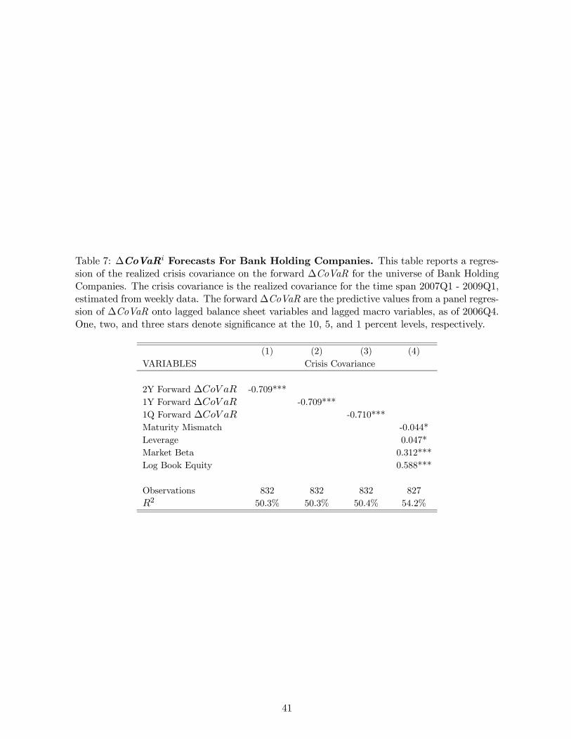
[Table 7 here]
Table 7 shows that the forward ∆CoVaR as of the end of 2006 was able to explain a little bit
over 50% of the cross sectional covariance during the crisis. We view this result as a very strong
one. Comparison of columns (1)-(3) shows that the forward horizon did not matter much in
terms of cross sectional explanatory power. Furthermore, column (4) shows that the information
contained in the estimated forward measures captures most of the ability of firm characteristics
to predict crisis covariance, as the individual characteristics only generate a slightly higher -
squared statistic. The forward ∆CoVaR thus summarizes in a single variable for each firm the
extent to which it is expected to contribute to future systemic risk.
5 Conclusion
During financial crises or periods of financial intermediary distress, tail events tend to spill across
financial institutions. Such spillovers are preceded by a risk-buildup phase. Both elements are
important contributors to financial system risk. ∆CoVaR is a parsimonious measure of systemic
risk that complements measures designed for individual financial institutions. ∆CoVaR broadens
risk measurement to allow a macroprudential perspective. The forward-∆CoVaR is a forward
looking measure of systemic risk contribution. It is constructed by projecting ∆CoVaR on
lagged firm characteristics such as size, leverage, maturity mismatch, and industry dummies.
This forward looking measure can potentially be used in macroprudential policy applications.
25
References
Acharya, V. (2009): “A Theory of Systemic Risk and Design of Prudential Bank Regulation,”
Journal of Financial Stability, 5(3), 224 — 255.
Acharya, V., L. Pedersen, T. Philippon, and M. Richardson (2010): “Measuring Sys-
temic Risk,” NYU Working Paper.
Adams, Z., R. Füss, and R. Gropp (2010): “Modeling Spillover Effects Among Financial In-
stitutions: A State-Dependent Sensitivity Value-at-Risk (SDSVaR) Approach,” EBS Working
Paper.
Adrian, T., and H. Shin (2010a): “The Changing Nature of Financial Intermediation and the
Financial Crisis of 2007-2009,” Annual Review of Economics, (2), 603—618.
Adrian, T., and H. S. Shin (2010b): “Liquidity and Leverage,” Journal of Financial Inter-
mediation, 19(3), 418—437.
Allen, F., A. Babus, and E. Carletti (2010): “Financial Connections and Systemic Risk,”
European Banking Center Discussion Paper.
Bassett, G. W., and R. Koenker (1978): “Asymptotic Theory of Least Absolute Error
Regression,” Journal of the American Statistical Association, 73(363), 618—622.
Bhattacharya, S., and D. Gale (1987): “Preference Shocks, Liquidity and Central Bank
Policy,” inNew Approaches to Monetary Economics, ed. byW. A. Barnett, and K. J. Singleton.
Cambridge University Press, Cambridge, UK.
Billio, M., M. Getmansky, A. Lo, and L. Pelizzon (2010): “Measuring Systemic Risk in
the Finance and Insurance Sectors,” MIT Working Paper.
Bodie, Z., D. Gray, and R. Merton (2007): “New Framework for Measuring and Managing
Macrofinancial Risk and Financial Stability,” NBER Working Paper.
Borio, C. (2004): “Market Distress and Vanishing Liquidity: Anatomy and Policy Options,”
BIS Working Paper 158.
Brady, N. F. (1988): “Report of the Presidential Task Force on Market Mechanisms,” U.S.
Government Printing Office.
Brunnermeier, M., and Y. Sannikov (2009): “A Macroeconomic Model with a Financial
Sector,” Princeton University Working Paper.
Brunnermeier, M. K. (2009): “Deciphering the Liquidity and Credit Crunch 2007-08,” Jour-
nal of Economic Perspectives, 23(1), 77—100.
Brunnermeier, M. K., and P. Cheridito (2011): “Systemic Risk Charges,” Princeton Uni-
versity working paper.
Brunnermeier, M. K., A. Crocket, C. Goodhart, A. Perssaud, and H. Shin (2009):
The Fundamental Principles of Financial Regulation: 11th Geneva Report on the World Econ-
omy.
26
Brunnermeier, M. K., and L. H. Pedersen (2009): “Market Liquidity and Funding Liq-
uidity,” Review of Financial Studies, 22, 2201—2238.
Caballero, R., and A. Krishnamurthy (2004): “Smoothing Sudden Stops,” Journal of
Economic Theory, 119(1), 104—127.
Cao, Z. (2010): “Shapley Value and CoVaR,” Bank of France Working Paper.
Chernozhukov, V., and S. Du (2008): “Extremal Quantiles and Value-at-Risk,” The New
Palgrave Dictionary of Economics, Second Edition(1), 271—292.
Chernozhukov, V., and L. Umantsev (2001): “Conditional Value-at-Risk: Aspects of Mod-
eling and Estimation,” Empirical Economics, 26(1), 271—292.
Claessens, S., and K. Forbes (2001): International Financial Contagion. Springer: New
York.
Danielsson, J., and C. G. de Vries (2000): “Value-at-Risk and Extreme Returns,” Annales
d’Economie et de Statistique, 60, 239—270.
Engle, R. F., and S. Manganelli (2004): “CAViaR: Conditional Autoregressive Value at
Risk by Regression Quantiles,” Journal of Business and Economic Statistics, 23(4).
Estrella, A. (2004): “The Cyclical Behavior of Optimal Bank Capital,” Journal of Banking
and Finance, 28(6), 1469—1498.
Gauthier, C., A. Lehar, and M. Souissi (2009): “Macroprudential Capital Requirements
and Systemic Risk,” Bank of Canada Working Paper.
Geanakoplos, J., and H. Polemarchakis (1986): “Existence, Regularity, and Constrained
Suboptimality of Competitive Allocation When the Market is Incomplete,” in Uncertainty,
Information and Communication, Essays in Honor of Kenneth J. Arrow, vol. 3.
Giglio, S. (2011): “Credit Default Swap Spreads and Systemic Financial Risk,” working paper,
Harvard University.
Gordy, M., and B. Howells (2006): “Procyclicality in Basel II: Can we treat the disease
without killing the patient?,” Journal of Financial Intermediation, 15, 395—417.
Gorton, G., and A. Metrick (2010): “Haircuts,” NBER Working Paper 15273.
Gray, D., R. Merton, and Z. Bodie (2007): “Contingent Claims Approach to Measuring
and Managing Sovereign Credit Risk,” Journal of Investment Management, 5(4), 5—28.
Hartmann, P., S. Straetmans, and C. G. de Vries (2004): “Asset Market Linkages in
Crisis Periods,” Review of Economics and Statistics, 86(1), 313—326.
Huang, X., H. Zhou, and H. Zhu (2010): “Measuring Systemic Risk Contributions,” BIS
Working Paper.
Jorion, P. (2006): “Value at Risk,” McGraw-Hill, 3rd edn.
Kashyap, A. A., and J. Stein (2004): “Cyclical Implications of the Basel II Capital Stan-
dards,” Federal Reserve Bank of Chicago Economic Perspectives, 28(1).
27
Koenker, R. (2005): Quantile Regression. Cambridge University Press: Cambridge, UK.
Koenker, R., and G. W. Bassett (1978): “Regression Quantiles,” Econometrica, 46(1),
33—50.
Korinek, A. (2010): “Systemic Risk-taking: Amplification Effects, Externalities and Regula-
tory Responses,” University of Maryland Working Paper.
Kupiec, P. (2002): “Stress-testing in a Value at Risk Framework,” Risk Management: Value
at Risk and Beyond.
Lehar, A. (2005): “Measuring systemic risk: A risk management approach,” Journal of Bank-
ing and Finance, 29(10), 2577—2603.
Lorenzoni, G. (2008): “Inefficient Credit Booms,” Review of Economic Studies, 75(3), 809—
833.
Manganelli, S., T.-H. Kim, and H. White (2011): “VAR for VaR: Measuring Systemic
Risk Using Multivariate Regression Quantiles,” unpublished working paper, ECB.
Rubin, R. E., A. Greenspan, A. Levitt, and B. Born (1999): “Hedge Funds, Leverage,
and the Lessons of Long-Term Capital Management,” Report of The President’s Working
Group on Financial Markets.
Segoviano, M., and C. Goodhart (2009): “Banking Stability Measures,” Financial Markets
Group Working Paper, London School of Economics and Political Science.
Stein, J. (2009): “Presidential Address: Sophisticated Investors and Market Efficiency,” The
Journal of Finance, 64(4), 1517—1548.
Stiglitz, J. (1982): “The Inefficiency of Stock Market Equilibrium,” Review of Economic
Studies, 49, 241—261.
Tarashev, N., C. Borio, and K. Tsatsaronis (2009): “The systemic importance of financial
institutions,” BIS Quarterly Review.
Wong, A., and T. Fong (2010): “An Analysis of the Interconnectivity among the Asia-Pacific
Economies,” Hong Kong Monetary Authority Working Paper.
28
Appendices
A CoVaR Estimation via Quantile Regressions
This appendix explains how to use quantile regressions to estimate VaR and CoVaR. Suppose
that returns have the following linear factor structure
= 0 +−11 +
2 +¡3 +−14 +
5¢ (10)
where −1 is a vector of state variables. The error term is assumed to be i.i.d. with zero
mean and unit variance and is independent of −1 so that h |−1
i= 0. Returns are
generated by a process of the “location scale” family, so that both the conditional expected return
h
|−1
i= 0+−11+
2 and the conditional volatility −1h
|−1
i=¡
3 +−14 +5¢depend on the set of state variables−1 and on
. The coefficients 0
1, and 3 could be estimated consistently via OLS of on −1 and
. The predicted value
of such an OLS regression would be the mean of conditional on −1 and
. In order to
compute the VaR and CoVaR from OLS regressions, one would have to also estimate 3, 4 and
5, and then make distributional assumptions about .14 The quantile regressions incorporate
estimates of the conditional mean and the conditional volatility to produce conditional quantiles,
without the distributional assumptions that would be needed for estimation via OLS.
Instead of using OLS regressions, we use quantile regressions to estimate model (10) for
different percentiles. We denote the cumulative distribution function (cdf) of by ¡¢, and
its inverse cdf by −1() for percentile . It follows immediately that the inverse cdf of
is
−1
¡|−1
¢= +−1 +
, (11)
where = 0 + 3−1(), = 1 + 4
−1(), and = 2 + 5
−1() for quantiles
∈ (0 1). We call −1
¡|−1
¢the conditional quantile function. From the definition of
14The model (10) could otherwise be estimated via maximum likelihood using a stochastic volatility or GARCH
model if distributional assumptions about are made. The quantile regression approach does not require specific
Real Estate Excess Return -0.081 2.8 -14.5 21.330 -4.0
Table 2: Summary Statistics for Estimated Risk Measures. The table reports summary
statistics for the asset returns and 1% risk measures of the 1226 financial firms for weekly data
from 1986Q1-2010Q4. denotes the weekly market-valued asset returns for the firms. The
individual firm risk measures and the system risk measure are obtained by
running 1-% quantile regressions of returns on the one-week lag of the state variables and by
computing the predicted value of the regression. ∆ is the difference between 1% − and the 50% − , where − is the predicted value from a − %quantile regression of the financial system asset returns on the institution asset returns and on
the lagged state variables. The stress ∆ is the ∆ computed with the worst 1%
of state variable realizations and the worst 1% financial system returns replaced in the quantile
regression. All quantities are expressed in units of weekly percent returns.
Variable Mean Std. Dev. Obs.
(1) 0.34 7.3 791231
(2) -12.17 8.00 790868
(3) ∆ -1.16 1.30 790868
(4) Stress-∆ -3.22 3.86 790868
(5) -6.24 3.53 1226
37
Table 3: Average t-Statistics of State Variable Exposures. The table reports average t-
statistics from 1%-quantile regressions. For the risk measures and the system risk measure
, 1-% quantile regressions are run on the state variables. For , 1-% quantile
regressions of the financial system returns are run on the state variables and the firms’ asset
returns.
Variable VaR VaR CoVaR
VIX (lag) (-16.18) (-13.14) (-20.76)
Repo spread (lag) (-6.77) (-0.84) (-7.18)
Three month yield change (lag) (-1.85) (-0.69) (-2.38)
Table 7: ∆CoVaR Forecasts For Bank Holding Companies. This table reports a regres-
sion of the realized crisis covariance on the forward ∆CoVaR for the universe of Bank Holding
Companies. The crisis covariance is the realized covariance for the time span 2007Q1 - 2009Q1,
estimated from weekly data. The forward∆CoVaR are the predictive values from a panel regres-
sion of ∆CoVaR onto lagged balance sheet variables and lagged macro variables, as of 2006Q4.
One, two, and three stars denote significance at the 10, 5, and 1 percent levels, respectively.
(1) (2) (3) (4)
VARIABLES Crisis Covariance
2Y Forward ∆ -0.709***
1Y Forward ∆ -0.709***
1Q Forward ∆ -0.710***
Maturity Mismatch -0.044*
Leverage 0.047*
Market Beta 0.312***
Log Book Equity 0.588***
Observations 832 832 832 827
2 50.3% 50.3% 50.4% 54.2%
41
Table 8: ∆CoVaR Forecasts using GARCH estimation. This table reports the coef-
ficients from forecasting regressions of the two estimation methods of 5% ∆CoVaR on the
quarterly, one-year, and two-year lag of firm characteristics. The methodology for computing
the quantile regression ∆CoVaR is given in the captions of Tables 2 and 3. FE denotes fixed
effect dummies. The GARCH ∆CoVaR is computed by estimating the covariance structure of
a bivariate diagnonal VECH GARCH model. All regressions include time effects. In this table
VaR is estimated using a GARCH(1,1) model. Newey−West standard errors allowing for up tofive periods of autocorrelation are dispalyed in parentheses. One, two, and three stars denote
significance at the 10, 5, and 1 percent levels, respectively.
Table 9: ∆CoVaR Forecasts using alternative system returns variable. This table re-
ports the coefficients from forecasting regressions of the two estimation methods of 5%∆CoVaR
on the quarterly, one-year, and two-year lag of firm characteristics. In the columns labeled
, ∆CoVaR is estimated using the regular system returns variable described in Section
3, while in columns labeled −, ∆CoVaR is estimated using a system return variable
that does not include the firm for which ∆CoVaR is being estimated. The methodology for
computing the quantile regression ∆ CoVaR is given in the captions of Tables 2 and 3. FE
denotes fixed effect dummies. All regressions include time effects. Newey−West standard errorsallowing for five periods of autocorrelation are displayed in parentheses. One, two, and three
stars denote significance at the 10, 5, and 1 percent levels, respectively.