Page 1
National Institute for Higher Education, Dublin
School of Electronic Engineering
Thesis Submitted for Degree of Masters of Engineering
VOWEL CODING USING AN ARTICULATORY
The research contained herein was completed by me, the undersigned.
MODEL
By
Mary Murphy B.E. (Elee)
Submitted to
Dr. Sean Marlow B.Sc. PhD.
September 1988
Page 2
TABLE OF CONTENTS
Abstract
Acknowledgements
1. Introduction
1.1 Coding of Speech at Low Bit Rates
1.2 Vocoders 4
1.3 Articulatory Vocoders 5
1.4 Thesis Overview 7
2. The Mechanism of Speech Production 8
2.1 Introduction 8
2.2 Human Speech Production 8
2.2.1 Voice source Generation 9
2.2.1 Articulation 9
2.3 Models for Speech Production 11
2.3.1 Source Models 11
2.3.2 Articulatory Models 13
2.4 The ASY Synthesiser 13
2.4.1 Meimelstein’s Model 14
2.4.2 Source Excitation for ASY 15
3. Sound Propogation in the Vocal Tract 17
3.1 Introduction 17
3.2 Sound Propogation 17
3.2.1 Transfer Function in the Sampled
Time Domain 20
Page 3
3.3 Transfer Function of the ASY synthesiser 21
Linear Predictive Coding of Speech
4.1 Introduction 23
4.2 LPC Model for Speech Production 23
4.3 Solution of LPC 27
4.3.1 Prony’s Method 27
4.3.2 Autocorrelation Method 29
4.3.2.1 Solution of the Autocorrelation
Method 30
4.3.2.2 Choice of Window 31
4.3.3 Covariance Method 31
4.3.3.1 Solution of the Covariance
Method 32
4.3.4 PARCQR Analysis (Lattice Method) 33
4.4 Relationship between PARCOR Analysis and
the Acoustic Tube Model 35
Estimation of the Vocal Tract Transfer Function
5.1 Introduction 37
5.2 A New Model of Speech Production 37
5.3 Methods for extracting the Vocal Tract
Transfer Function 39
5.3.1 Inverse Filtering Methods 39
5.3.1.1 Experimental Procedures 42
5.3.2 Covariance over the Closed Glottis
Interval 45
5.3.2.1 Existing Methods for obtaining
Glottal Closure 46
Page 4
5.3.2.2 Algorithm for Extracting Optimum
Location 50
5.3.2.3 Experimental Procedures 52
5.4 Extraction of Glottal Parameters 55
5.5 Experimental Results and Conclusions 57
5.5.1 Comparison of Preemphasis Methods 57
5.5.2 Comparison of CGI and First-Order
Preemphasis Methods 62
5.5.3 Explanation of Results 74
5.3.3.1 Autocorrelation vs. Covariance
Methods 74
5.5.3.2 Source-Tract Interaction 74
Articulatory Speech Coding
6.1 Introduction 77
6.2 General Speech Coding System 77
6.3 Quantization 78
6.3.1 Vector Quantization 79
6.4 Distortion Measures 80
6.4.1 Distortion Measures Based on the Mean
Squared Error 81
6.4.2 Distortion Mesures Based on the Weighted
Mean Squared Error 83
6.4.3 Itakura-Saito Distortion Measure 83
6.5 Articulatory Speech Coding System 84
6.6 Generation of the Articulatory Codebook 86
6.6.1 Sensitivity Analysis Method 86
6.6.2 Limitations of the Sensitivity Analysis
Method 87
Page 5
6.7 Linked Codebook Generation 88
6.8 Evaluation of Distortion Measures
6.9 Glottal Codebook Design 94
6.6.3 Training Set Method 88
89
7. Estimation of Articulatory Parameters from the Speech Wave
7.1 Introduction 95
7.2 Inverse Problem of the Vocal Tract 95
7.2.1 Regression Analysis 96
7.2.2 Constrained Optimization 96
7.3 Shirai’s Method 97
7.4 Application of Shirai’s Method 99
7.4.1 Minimization Algorithm 100
7.4.1.1 Adaptation of Mermelstein’s
Model 101
7.4.1.2 Choice of Initial Estimate
7.4.1.3 Choice of Weighting Matrices
7.4.1.4 Computation of derivative of
h(x) 102
7.4.1.5 Choice of Acoustic Parameters
7.4.1.6 Convergence Criteria 103
7.5 Analysis Results and Possible Improvements
95
101
102
103
103
8. Discussion, Improvements and Conclusions 106
8.1 Convergence Techniques 106
8.2 Bit Rates 106
8.3 Resources and Computation 107
8.4 Recording Conditions 107
8.5 Sampling Rate 108
Page 6
8.6 Limitations of CGI / Alternatives
8.7 Completion of Articulatory Vocoder
8.8 Conclusions 109
References
Page 7
ABSTRACT
An investigation into articulatory vocoding for vowels, as a means of achieving high quality coding at low bit rates, is carried out in this thesis. Methods of estimating the vocal tract transfer function from thespeech wave are compared, and an algorithm for closed glottis interval(CGI) analysis is developed. CGI analysis is chosen over autocorrelationbased inverse filtering methods.
Various distortion measures for use in Vector Quantization are evaluated,and a new covariance distortion measure is proposed. It is shown that this measure yields close matches from an acoustic codebook.
An articulatory coding system is designed, including a linked codebook of articulatory shapes, based on synthetic speech. A method of generating a similar codebook from real speech is proposed, and an investigation into estimating articulatory parameters from the speech wave is carried out to this end.
1
Page 8
ACKNOWLEDGEMENTS
Much thanks to my supervisor, Dr. Sean Marlow, for his advice and encouragement during the last two years. I would also like to thank Dr. Ronan Scaife of UCG for providing the ASY synthesiser, and Dr. Frank Owens and Sean Murphy of the University of Ulster, Jordanstown for helping me obtain speech data. Thanks to all my fellow Post-Grads for the crack, coffee, pool and crosswords, and finally to my parents, without whom this would never have been written.
2
Page 9
CHAPTER 1 INTRODUCTION
Despite the fact that high bandwidth channels and networks are becoming more
viable, coding speech at low bit rates has retained its importance. Specific
applications include:
(i) Digital encryption i.e. situations where high security is required over
low data rate channels such as radio links.
(ii) Cases where memory efficient systems for voice storage e.g. voice mail
are required.
(iii) Mobile telephony, In this case more users can be accommodated on
cellular radio or satellite links.
Developers of digital speech coders strive to optimize the interplay of four
parameters: bit rate, quality, complexity and delay time. As bit rate is reduced,
quality naturally drops off, unless complexity is increased. At high bit rates e.g.
64Kb/s, used in pulse code modulation, quality is not a problem, but it is
believed that high quality coding may eventually be practical at rates as low as
2Kb/s [4].
There are two main types of coders:
(i) Waveform coders, which attempt to send an approximation of the
speech signal,
(ii) Vocoders (Voice Coders), which attempt to model the speech
production mechanism directly, and send parameters which accurately
describe the speech production process.
Vocoders results in a drastic reduction in bit rates, and are of primary importance
for speech coding,
1.1 Coding of Speech at low bit rates
3
Page 10
1,2 Vocoder
In the basic vocoder synthesiser, it is assumed that speech is generated by a vocal
tract filter being excited by either a regular pulse source or random noise.
Spectral coefficients specifying the vocal tract filter response define the speech
formants, while pitch and voicing are defined by the pitch value and a binary
voiced / unvoiced decision to select the source of excitation.
There are two main types of vocoders:
(i) Channel Vocoders: In this type, typified by Holmes [1], there are
typically 15-20 channels, each being a spectrum analyser consisting of
a bandpass filter, a rectifier and a low pass filter. These are used to
determine the spectral shape.
(ii) LP (Linear Predictive) Vocoders: This type is based on linear
predictive coding (LPC), a speech analysis method first introduced by
Atal et al. [2]. Coefficients of an N-pole digital filter, determined
from LPC analysis, are used to describe the speech.
In both cases, a pitch value and voicing parameter are extracted simultaneously.
In general, speech quality for the two types are comparable with the signal
processing required somewhat greater for the channel type [3].
Features of the above basic vocoder types impose fundamental limitations on the
speech quality obtainable. The main restricting features are:
(i) Regular pulses for the voiced excitation
(ii) Binary voicing decision - the synthesised speech can only be purely
voiced or unvoiced.
Both the above lead to an artificial quality. It is generally agreed that LPC is
based on a clearly oversimplified model of the voice source [5], although this
Page 11
simplification gives the advantage that a direct and efficient analysis can be used.
1.3 Articulatory Vocoders
An alternative approach to the general vocoder approach design is to use
articulatory parameters for coding speech. As well as providing an economical
description of speech, an articulatory vocoder has the following advantages over
traditional vocoders:
(i) Articulatory parameters model speech production directly, thus inherently
incorporating physiological constraints that exist in the human vocal
tract. For example, transitional effects due to tongue and jaw inertia
may be modelled directly. An articulatory synthesiser has the potential
to produce natural sounding speech at bit rates below 4800b/s.
(ii) The coding (including excitation) parameters have a physiological base
and vary slowly. A parametric model of voiced excitation i.e. a
glottal source model is usually incorporated in an articulatory vocoder.
This overcomes the disadvantages of a binary voicing decision.
(iii) Interpolation between parameters (shapes) result in physically realisable
inteirnediate shapes, which is not always the case for LPC parameters.
Slightly erroneous parameters do not usually result in unnatural speech.
Flanagan [3] has extolled the possibilities of an articulatory vocoder, and
recommended it above other types. However, the success of an articulatory
vocoder is dependent on how accurately articulatory data may be obtained from
the speech signal. Much research has been done into this problem, however
results have mainly been used for speech recognition, and surprisingly little
knowledge has been applied to articulatory vocoding. The simplest type of
articulatory vocoders use area functions obtained from direct speech analysis (LPC)
as the parameters, which offers no significant advantage over traditional vocoder
types. At the other end of the scale is a vocoder recently developed by Sondhi
5
Page 12
types. At the other end of the scale is a vocoder recently developed by Sondhi
et al„ based on their extremely complex speech synthesiser [4], the parameters of
which are difficult to obtain from the speech signal. One of the main problems
of this type is that its voicing parameters have a physiological base, the detail of
which introduces many problems for speech analysis.
To extract the source excitation (glottal signal), the vocal tract model estimated
from the speech wave must be very accurate. Thus a method which extracts the
true glottal waveform would simultaneously extract excellent parameters to
represent the vocal tract transfer function. From these vocal tract parameters an
accurate representation of the vocal tract shape, and hence positions of the
articulatory organs may be estimated.
1.4 Thesis Overview
In this thesis, a compromise between the two extreme articulatory vocoder types is
proposed, and a quality articulatory vocoder for vowels sounds is designed. The
glottal waveform is extracted from the speech wave by a technique generally
known as glottal inverse filtering. Specifically, this involves a modified type of
linear predictive analysis. Conventional LPC methods are first detailed, and from
these, methods for extracting an accurate vocal tract shape for vowels are
developed and compared. Closed glottal interval covariance analysis is
investigated, and a new improved algorithm is presented for the method. This
method is compared to pitch synchronous and asynchronous analyses which use the
autocorrelation method with various types of preemphasis.
The application of vector quantization to articulatory coding is then discussed, and
a comparison of suitable distortion measures undertaken. A distortion measure,
based on one developed for the autocorrelation method of LPC, but modified for
the covariance method, is then proposed. The results of the comparisons are later
taken into account in determining the best acoustic match for constructing a
6
Page 13
codebook.
The construction of an articulatory codebook, and methods for quantizing
articulatory parameters are discussed. The idea of a linked codebook of acoustic
and articulatory parameters is presented, and one is generated, based on synthetic
speech. A natural follow-on, using real speech, is proposed, and methods for
constructing such a codebook discussed. This prompts a discussion on methods of
obtaining the articulatory parameters directly from the speech wave, and one of
these methods is investigated in detail.
Finally, methods for improving the existing set-up are proposed, and possibilities
of its extension to other types of speech sounds are outlined. Directions for
future research are proposed.
7
Page 14
2. THE MECHANISM OF SPEECH PRODUCTION
2.1 introduction
In this chapter, the human physiological speech production process in relation to
vowels, is presented. The generation of voiced source excitation, and the
articulation process are discussed. Articulatory models, which attempt to model
this process to reproduce the acoustic speech waveform, are reviewed. Finally, an
introduction to ASY, the articulatory synthesiser used in this research, is presented.
This chapter forms the background to Chapter 3, which examines the acoustic
process of speech production.
2.2 Human speech production
Voiced speech waveforms are generated by a speech production process consisting
of two main parts:
(i) Voice source generation
(ii) Articulation
The machinery involved is shown in Fig 2.1.
Fig. 2.1 The human speech production mechanism [3]
8
Page 15
12A Yoicg-Sourgg Generation
The energy source for speech production is the respiratory system pushing air out
of the lungs. The air passes through the trachea and vocal cords of the larynx
into the pharynx (throat cavity) and mouth. The voiced sounds of speech are
produced by the vibratory action (i.e. phonation) of the vocal cords. The larynx
is also known as the voice box, as its purpose is to hold the vocal cords in the
correct position and tension for phonation. The orifice between the cords is
known as the glottis. The vocal cords are suspended within a cage of cartilage,
and by using a set of muscles attached to this cartilage, they can be moved as
required. The action proceeds as follows:
Assume initially that the cords are together. The subglottal pressure increases,
forcing them apart. As the air flow through the cords increases, the local
pressure drops, according to the Bemouilli effect, and this results in the cords
being sucked together again. Thus quasi periodic pulses of air excite the vocal
tract for voiced sounds.
The pitch (frequency of oscillation) depends on both the vocal cord tension and
their mass per unit length. The volume of air through the glottis as a function
of time is roughly proportional to the area of glottal opening. The waveforms are
approximately triangular in shape, and typical duty cycles (i.e. ratio of open time
to total period) are of the order of 0.3 to 0.7. The glottal waveform shape
varies greatly for a given individual, depending on sound pitch and intensity. The
pitch normally ranges from 50 - 200Hz for men, with women and children an
order of an octave higher.
2,2.2- Articulation
The vocal tract is a nonuniform acoustic tube formed by the articulatory organs,
It begins at the glottis and ends at the mouth. It is connected to the nasal tract,
which stretches from the velum to the nostrils. The velum controls the acoustic
9
Page 16
coupling between the tracts, i.e. when it is open the tracts are coupled
acoustically, and nasalized sounds are produced. The tract accentuates certain
frequencies by resonance, producing each sound with an individual quality. This
process is called articulation.
From observation, vowel sounds are dependent on the vocal tract shape as a
whole, and may be characterised by three parameters:
(i) the minimum cross-section area, usually at the tongue hump
(ii) the distance of (i) from the glottis, and
(iii) the magnitude of the lip opening.
F!g 22 Corresponding positions in die tract for vowels in the words: (1)
"heed", (2) "hid", (3) "head", (4) "had", (5) "hod", (6) "hawed". (7)
"hood", (8) "who’d" [5]
These characteristic shapes are produced by the movement of a combination of
articulators, i.e. the tongue, jaw, lips, and to a lesser extent the velum. The
position of the tongue separates vowels into front/back and high/low classifications.
Klatt [6] also used a lip classification i.e. rounded/unrounded. For nonnazalized
Page 17
voice sounds, the velum is closed. The physiological basis for these
classifications may be seen in Fig 2.2. A rapid transition from one vowel to
another is known as a dipthong.
Following articulation, the speech is radiated at the mouth. The acoustic
consequences of lip radiation are discussed in Chapter 3.
2.3 Models for speech productioa
All speech utterances, however varied, have one unifying factor - their origin, the
human speech production process. For this reason, the advantages of mimicking
this process are many - such problems as speaker differences, accents and
coarticulation effects may be overcome by accurate modelling. Hence speech
production modelling is a very active area of speech research, contributing to more
natural sounding speech synthesis, better recognition rates, and improved coding
quality. Models for speech production consist of two parts, the excitation of the
vocal cords, and the articulators of the tract.
2.3.1 Source models
Source models vary greatly in detail and accuracy. The most realistic
physiologically based model of the vocal cords is Ishizaka and Flanagan’s two
mass model [7], shown in Fig 2.3.
LUNGS TRACHEA VOCAL VOCAL TR A CT MOVTHM O N CH I COROS
Fig 2.3 Flanagan’s Two - Mass Model [7]
11
Page 18
The model is a non-linear system, dependent on the supraglottal pressure in the
vocal tract. Thus, it accounts for the interaction between the glottal volume
velocity and the input impedance of the vocal tract. Each vocal cord is described
by two masses, with associated stiffnesses and losses. For voiced sounds
SuR, . u + L. . — -£ = P - P , (2. 1)t ot g 8 t s i v '
where Ps is the lung (subglottal) pressure, P 1 is the supraglottal (vocal tract)
pressure, and Ug is the volume velocity. Rtot and are the total
quasi-stationary resistance and inductance representing the expansion and contraction
of the vocal cords and are dependent on both the glottal area and the area of the
first section of the vocal tract.
The model parameters are the lung pressure, vocal cord tension, and glottal
opening area. Both the pitch and glottal waveform are dependent on the lung
pressure and glottal rest area. The pitch is controlled by the vocal cord tension.
The effect of the acoustic properties of the trachea and lungs have been shown to
be minor by Wakita and Fant [8], and are ignored. Experiments with one-mass
models found that the source tract interaction was very dependent on the assumed
intraglottal pressure distributions [3], while experments with multi-mass models [10]
found they were no better than the two-mass model, in fact they overemphasised
source tract interaction.
While this model produces very natural sounding speech, and is the most accurate
developed, limited knowledge of the voice anatomy and the difficulties of
obtaining the model parameters from the speech wave has meant that more
simplified glottal models are often used. These model the glottal waveform, rather
than its physiological base [10].
12
Page 19
2.3.2 Articulately models
The design of articulatory models i.e. those which attempt to model the movement
of articulators directly, has always been a prominent area of speech research. The
first articulatory model of significance was developed by Stevens and House [11],
who presented the three parameter model described earlier, representing the vocal
tract shape for English vowels. Using this, Fant [12] attempted to reconstruct
speech spectra based on X-ray data for Russian vowels.
Initially, tract models for speech synthesis [13] used area functions as input.
Following the success of Stevens and House, however, models controlled by
articulators have been developed. This approach supports the view that the value
of an articulatory model is to what extent it can produce significant detail in its
output from simple inputs. Articulator movements try to match the vocal tract
shape rather than resolve individual muscles. For the generation of most
articulatory shapes, a model with seven to ten degrees of freedom should suffice.
Coker’s model [14] uses independent and semi-independent articulators, e.g. (tongue
tip relative to tongue body). A target approach is used where the motion of each
articulator is characterized by a time constant dependent on its weight and the
available muscular forces. Like Coker’s model, Mermelstein’s [15] attempts to
match real X-ray data. Although similar in many respects, each places a different
emphasis on speech production. Coker’s, through incorporating a dynamic
controller, stresses synthesis by rule, while the latter concentrates on interactive
and systematic control of articulatory configurations and the subsequent acoustic
and perceptual effects.
2.4 The ASY Synthesiser
AS Y, the research synthesiser developed by Rubin and Baer [16] using
Mermelstein’s model, is used in this project.
13
Page 20
The movable articulators in this model (see Fig 2.4), are the tongue, jaw, lips,
velum and hyoid.
2.4.1 Mermelstein’s Model
Fig 2.4 Mermelstein’s Model
These are surrounded by a fixed structure consisting of the rear pharyngeal wall
and the maxilla, which limits the range of the articulators for consonant
articulations. The emphasis when developing the model was manual matching
with X-ray tracings obtained from Perkell [17]. The specification of the key
articulator positions completely determines the vocal tract outline. These are
described as follows:
(i) The jaw is defined by its location, J, (in polar coordinates Sj and 0j)
relative to to the fixed point F ; Sj is usually constant.
(ii) The hyoid has horizontal and vertical coordinates at point H, such that
below H the curve is a function of H alone. The hyoid does not
move much for vowels.
(iii) The tongue body outline is represented by a circle of moving centre
Page 21
and fixed radius, with polar coordinates (sc and 0C) referenced to FJ.
This makes its position dependent on jaw movement as well as moving
independently.
(iv) The tongue tip and blade move relative to the tongue body. The tip
appears to rotate about point B so is defined by polar coordinates (s
and 0t) relative to B. The blade outline is a curve represented by a
radial coordinate. For vowels, this is simplified, where it is effectively
only a function of jaw and tongue body coordinates.
(v) The lips open and protude relative to the jaw and maxilla. These
positions are described by the height and protrusion, respectively
and pi.
(vi) The velum opens for nasals, and may be ignored for vowel
production.
The anterior outline of the pharynx was observed to be controlled by the hyoid
and tongue body positions and this is incorporated in the model. The rigid outline
was accurately matched with X-ray tracings. By imposing a grid structure on the
resulting outline, the area of function of the tract may be determined, with the
help of previously published data to closely match the vocal tract shape. Section
lengths of 0,875cm are produced, with the number of discrete area sections (and
hence vocal tract length) dependent on the particular configuration. The acoustic
properties of the synthesiser (i.e. its transfer function) are discussed in section 3.3
2.4.2 Source Excitation for ASY
A time domain acoustic waveform, representing Ug, is used to excite the vocal
tract, which can be represented by time varying parameters. These parameters are
based on the Rosenberg model [18] of glottal pulse excitation, shown in Fig 2.5,
and are:
15
Page 22
(i) pitch period T ( = 1 / fundamental frequency),
(ii) amplitude a,
(iii) duty cycle i.e. ratio of open time to pitch period, = Tp/T
(iv) speed ratio i.e. ratio of rise time to fall time, = Tp/Tn
Fig 2.5 Model for the glottal pulse [18]
16
Page 23
3. SOUND PROROGATION IN THE VOCAL TRACT.
3.1 introduction
In this chapter, the acoustic properties of the vocal tract described in Chapter 2
are presented. Using various assumptions, the transfer function of the vocal tract
is derived, and reflection coefficents which describe the acoustic sound propogation
through the tube are derived in terms of the cross-sectional area of the tube. The
transfer function of the ASY synthesiser is then described.
3.2 Sound Propogation
To analyse the propogation of sound through it, the vocal tract is modelled as a
nonuniform, time-varying cross-section tube. For frequencies corresponding to
wavelengths that are long in comparison to the tract dimensions, plane wave
propogation of sound along its axis may be assumed. Assuming no viscous or
thermal conduction losses in the air or the tract walls, the sound waves in the
tube satisfy Portnoff’s equations [19]:
8p 8( u / A)- ---- = p (3.1a)
5x 8t
5u 1 5(u/A) SA
8x pc^ 8 t 5t(3.1b)
wherec = velocity of sound;
p = p(x,t) = variation in sound pressure, position x, time t;
u = u(x,t) = corresponding change in volume velocity;
p = density of air in tube;
A = A(x,t) = cross (X) - section area normal to axis of the tube.
Boundary conditions are imposed at either ends of the tube: accounting for sound
radiation at the lips and the nature of the excitation at the glottis.
17
Page 24
Closed form solutions of eqns. (3.1) are not possible, however numerical solutions
may be obtained. The area function A(x,t) must be known, whether from detailed
direct measurements, or from the speech wave. The solution is very
complicated, thus various assumptions are made.
The vocal tract is regarded as a series of tubes, each of constant cross-section.
As the vocal tract changes slowly, it is reasonable to assume the areas are
constant over a short space of time i.e. the analysis interval (20 - 30ms). Thus
for each section
A(x,t) = A = constant. (3.2)
Thus for the mth uniform tube, eqns. (3.1) are simplified into difference equations
to give a solution of the form:
um ( x , t ) = [ um ( t ■ x/ c ) ' % ^ + x/c) ] (3.3a)
Pm ( x , t ) = [ p* ( t - x/c) + p^ ( t + x/c) ] (3.3b)
which are interpreted as forward and backward travelling waves, with the centre of
each section defined as x = 0, as shown in Fig 3.1.
-£<* + *> t m(t - x) l-------> --------->
1 I
! um(t - T> ! "m<‘ + T> !1 <------ 11 1
<-------- 1
x = - 1/2 x = 0 x = 1/2l <---------------------------------- I >1
sectio n m< >g lo t t is lip s
Fig 3.1 Forward and reverse volume velocity waves in section m.
Page 25
From eqn. (3.3), and using Portnoff’s equations, a relationship between pressure
and volume velocity may be derived, i.e.
Pm ( x , t ) = pc . [ uffl ( t - x/c) - um"(t + x/c) ]
m
u + ( t - T )----- >
----- >
U B ( t ♦ l )<--------
V i < ‘ -<----------
section m- area Am a
section m-1area A,m- 1
g l o t t i s l i ps
(3.4)
Fig 3.2 Continuity conditions for volume velocity between section m and
section m - 1 .
Examining the continuity considerations between boundaries, shown in Fig 3.2,
and defining the time taken for a wave to propogate half way along a section as
21 / c (3.5)
it follows that
- u " ( t + t:) mm- 1
m-1
- • u +( t - t ), mm
(3.6)
19
Page 26
and from this a reflection coefficient may be defined:
A 1 Am-1 m /o *7\
•V ” A , - " A ( 3 -7)m- 1 m
or
Am 1 “
(3.8)A . 1 + um- 1 m
For the tubes at either end, boundary conditions are imposed. From Wakita [20],
the acoustic tube is assumed open at the lips, i.e. zero radiation impedance
Ho = 1 (3-9)
From this, the volume velocity at the lips is
uL( t ) = 2 u j ( t - x) (3.10)
At the glottis end, assuming a volume velocity Ug(t) with source impedance Zg,
the glottal area is defined as
pcAm = — (3.11)
g
3.2.1 Transfer function in the sampled time domain
The transfer function of the vocal tract will now be developed in terms of jx.
Defining
mcm = n (1 + |Xj) m > 0 , Cq = 1 (3.12a)
i =1
and
t = 2 (m + 1)t . (3.12b)m
20
Page 27
a new variable {y} is introduced such that
(3.13a)
(3.13b)
Sampling at T = 4x, manipulating and obtaining the Z - transforms of eqn (3.13)
results in
These expressions will be used to establish a relationship between the acoustic
tube model presented here and the LPC model of Chapter 4.
3.3 Transfer function of the ASY synthesiser
The transfer function for ASY is derived in a similar fashion to the model above.
However its boundary conditions are different, and it incorporates propogation
losses dependent on each X-section area. The attentuation (propogation loss) a is
defined as
Non ideal terminations are accurately accounted for. The radiation at the lips is
represented by a non-zero radiation impedance Zp which consists of a parallel RL
circuit i.e.
(3.14a)
and
(3.14b)
a l / 2 = 1 - 0.007 (A) 1 / 2 (3.15)
Z (3.16)r[ 2 / R + 0 .7 ( 1 - z ' 1 ) ]
21
Page 28
where
The glottal impedance Zg is modelled by a series RL circuit,where Rg and Lg
are dependent in the glottal area, and averaged over an interval, similar to the
glottal impedance discussed in Section 2.3.1. They are adjusted to account for
effects of yielding vocal tract walls. In the default state, Rg = 50Q and Lg =
1200i2
R = effective radius of lips = (A0 / it).
22
Page 29
4. LINEAR PREDICTIVE CODING OF SPEECH
fLl Introduction
In this chapter, the fundamental concept of Linear Predictive Coding (LPC) is
introduced, and its suitability to speech acoustics discussed. The basic equations
of LPC are derived, and various formulations are presented for their solution. In
particular, solutions for the autocorrelation and covariance methods are derived, and
the relationship between these and the lattice method derived. Then the lattice
formulation, by showing how the area functions of the vocal tract may be
obtained from its results, unifies the acoustic tube model of Chapter 3, and the
waveform analysis here. These solutions form the basis of the analysis of the
next chapter.
4.2 LPC Model for speech production
In order to efficiently analyse speech at an acoustic level, a knowledge of speech
production is essential. A suitable model of speech production is presented here
which leads to linear predictive analysis of the speech waveform.
Speech waveforms are the result of the vocal tract being acoustically excited. The
vocal tract may be represented by a slowly time varying linear filter. For most
sounds, particularly voiced, the tract changes slowly, and the speech may be
considered to be stationary over a short interval (e.g. up to 20ms). For this
reason, it may be modelled by a digital filter, whose parameters are updated at
regular at regular intervals. The tract is excited by the volume velocity waveform
from the glottis. In the case of voiced speech, this wave is smooth and periodic,
whereas for unvoiced speech, it corresponds to random white noise. This source -
filter model of speech production, shown in Fig 4.1, leads to a simple and
effective method of speech synthesis and coding.
23
Page 30
V O I C E D
4
V O C A L T R A C T
PARAMETERS
S k
G L O T T A L T I M E - V A R Y I N G> O s(n
E X C I T A T I O N^ D I G I T A L F I L T E R
■'WHITE"E X C I T A T I O N
Fig. 4.1 Source-Filter Model of Speech Production
For LPC, the model may be further simplified by representing the combined
spectral contributions of glottal flow, the vocal tract, and radiation at the lips into
a single time varying all pole filter (see Fig 4.2). The filter is excited by either
a series of periodic pulses generated by the vocal cords (in the case of voiced
speech), or random noise (unvoiced). Thus the difficult problem of separating the
source from the speech spectrum is bypassed.
IMPULSETRAIN
GENERATOR
SP ECT RAL E N V E L O P E
T I M E - V A R Y I N G^ A L L - P O L E ---------> s<n)
D I G I T A L F I L T E R
GRANDOMNGISE
GENERATOR
Fig. 4.2 Linear Prediction Model of Speech Production
Page 31
An all-pole filter model represents the vocal tract quite accurately and extra poles
compensate for zeros in the spectrum (which occur in nasals). By avoiding zeros,
the filter parameters may be readily determined.
Thus the transfer function of the all-pole filter is of the form
1
where {%} are the coefficients of the digital filter.
In the time domain, the speech samples s(n) are related to the excitation u(n) by
the simple difference equation
where G is the gain.
This is in the form of a linear predictor i.e. the essence of LPC is that, due to
the high correlation between adjacent speech samples, a sample s(n) may be
approximated as a linear combination of previous samples i.e.
H(z) (4.1)M -k
1 - I a^. zk=l
Ms(n) = E ak . s(n - k) + G u(n)
k=0
(4.2)
Ms(n) = I cx s(n - k)
k=0
(4.3)
Using this approximation, the prediction error is
Me(n) = s(n) - s(n) = s(n) - E a. s(n - k)
kk=0
(4.4)
If = ajC) then e(n) = G u(n) is the output of a system having transfer
Page 32
M - kA(z) = 1 - E a. . z (4.5)
k=l
and since e(n) = G u(n), the prediction error filter is an inverse filter for H(z)
1H(z) = (4.6)
A(z)
S(z)
function
= H(z) (4.7)E(z)
Thus the basic problem of LPC is to find a set of predictor coefficients which
minimise the mean squared error over a finite interval. These coefficients are
obtained by partially differentiating
E = E e (n ) 2 (4.8a)
i . e .
8E[ e(n) ]2 0 k _ j H (4.8b)
8ak
with respect to each % and setting the result equal to zero. This leads to a set
of simultaneous linear equations:
M Ek=0 nE a^ X s(n * k ) . s ( n - i ) = E s(n - i ) . s ( n ) , 1 à i é. M (4.9)
Defining
*P(i,k) = E s(n - i ) . s ( n - k) (4.10)n
26
Page 33
this can be simplified to
MI ak . V ( i , k ) = ‘P(i.O) 1 ^ i ± M (4.11)
k=l
4.3 Solution of LPC
Ideally, the mean squared error of eqn. (4.8) should be minimized over an infinite
interval, but this cannot be used in practise. The definition of the range of
minimization of the error leads to separate approaches to LPC. Many different
solutions exist for the solution of eqn. 4.11. Four are discussed in this research:
(i) Prony’s method [21]
(ii) Autocorrelation method [21,22]
(ii) Covariance method [23]
(iv) Lattice method [24]
4.11 .£c?n y X msttiod_
Prony’s method is very old, and is important in understanding linear prediction of
speech as it shows explicitly how the voiced speech model may be represented by
complex exponentials in the time domain.
The speech model during voicing corresponds to a sequence of unit samples
(separated by the pitch period) driving an all-pole filter 1/A(z). If transients from
preceding pitch periods are ignored, voiced speech samples during the period will
be proportional to the unit sample response of an all pole filter. Thus the sampled
speech data {s(n)J may be modelled as a linear combination of M complex
exponentials, i.e.
Ms(n) = Z u. ( z . ) (4.12)
i=l 1 1
where zj, i = 1„.M defines roots or zeros of A(z):
27
Page 34
A ( z j ) = 0 i = 1 , . ,M. (4.13)
E(z) 1S(z) = = (4.14)
A(z) A(z)
If speech were precisely representable by the model of eqn. (4.12), the unknowns
uj and Zj (2M in number) could be obtained by solving the set of 2M
simultaneous equations. Thus if a signal s(n) is composed of precisely M
complex exponentials, then 2M samples suffice to exactly determine the model
parameters.
As M becomes large, the solution to these equations becomes unwieldly. To
avoid solving them, another approach is :
S(z) A(z) = P(z) (4.15)
or
M M-lZ a. s(n - i ) = Z p. 8 . (4.16)
i =0 1 i =0 1 n,J
MZ a. s(n - i ) = 0 n = M,. . .N-l (4.17)
i =0 1
To account for the possibility that the model may not exactly represent a single
pitch period of real speech, an error term is introduced so
MZ a. s(n - i) = e(n) an = 1 (4.18)
i =0 1 u
With the driving sequence e(n) =
28
Page 35
So {aj} are obtained by minimizing the squared error a where
N-l -a = E e ( n r (4.19)
n=M
which will be shown to be the same result as the covariance method, hi this
case, zeros are also allowed i.e. P(z) is not necessarily equal to 1.
4.3.2 Autocorrelation method
In this method, the speech samples are assumed to be zero outside a certain
interval N, i,e. a windowing procedure is used:
stf(n) = s(n) . w(n) (4.20a)
where
w(n) = 0 n < 0 and n > N - 1 (4.20b)
In this case the limits of summation for E are
N+M-l .E = E e (n) (4.21)
n=0
It can be shown that 4/(i,k) = R(i-k) where R(k), the short time autocorrelation
function is defined as
N+M-lR(k) = E s ( n ) . s (n + k) (4.22)
n=0 w w
Since R(i-k) = R(k-i), eqn. (4,11) is simplified to
ME a . . R(i - k) = R ( i ) 1 4 i ^ M (4.23)
k=l K
29
Page 36
In matrix form this is
R(0) R(1) R(2) ......... - R(M-l) a l R(0 )R(l ) R(0) R(l) ......... R(M-2) a2 R(l)R(2) R(l) R(0) - - - - - - R(M-3) a 3 = R(2 )
R(M-l) R(M-2) R(M-3) -- R(0) R(M)
4.3.2.1 Solution of the autocorrelation method
The solution of eqn (4.23) is obtained by exploiting the fact that the
autocorrelation matrix is a Toeplitz matrix i.e. it is symmetric and all its elements
along a given diagonal are equal. Thus, an efficient algorithm may be used for
its solution. Many have been proposed [25,26], the most efficient being Durbin’s
recursive procedure [25]. This may be stated as follows:
E(0)= R(0) (4.25a)
k. = [ R(i) - V a ^ ^ R U - j ) ) / E(l_1) (4.25b)j=l J
a ^ = k. (4.25c)l i
aj i} = aj i l ) ' k i a i - j 1} (4.25d)
E( l ) = (1 - k . 2 ) . E(i_1) (4.25e)
Solving these equations recursively for 1 ^ i ^ M, the final solution is
a. = a^M) 1 ^ j ^ M (4.25f)J J J
The quantity E0) is the mean squared prediction error for a predictor of order i.
It can be shown [21] that the quantities kj are bounded by unity i.e.
1 ^ k i ^ 1 (4 .2 6 )
30
Page 37
and this is a necessary and sufficient condition for A(z) to be stable i.e. for all
its roots to be inside the unit circle.
4.3.2.2 Choice of Window
Because of its assumption of zero valued samples outside the analysis interval, the
autocorrelation method needs a window. The ideal window should have a high
frequency resolution (i.e. its main lobe should be narrow and sharp) and small
spurious distortion outside of this lobe (sharp drop off). A Hamming window [
27] is normally chosen as it has good frequency resolution and side lobes of less
than -40dB. It is of the form
w(n) = 0.54 - 0.46 * cos ( 2IIn / N - 1) 0 ^ n ^ N-l (4.27)
4.3.3 Covariance method
In this method, an interval of length N is also taken, but no assumptions are
made outside this interval, and no windowing is used. Thus E is taken over all
except the first M samples, so that samples outside the interval are not used i.e.
N-l 9E = Z e (n) (4.28)
n=M
Here 'F(i.k) becomes
N-l^ O . k ) = Z s (n - i ) . s (n + k) (4.29)
n=M
'F(i.k) is a cross-correlation function unlike the autocorrelation function used
earlier. From eqn (4,29), eqn. (4.11) may be written as
MZ a . T ( i , k ) = ¥ ( i , 0 ) (4.30)
k=l K
31
Page 38
which in matrix form is
¥(1,1) ¥(1,2) ........... ¥ ( 1 ,M) ' a l ¥ ( 1 ,0 )¥( 2 , 1 ) ¥ ( 2 ,2 ) ......... ¥ ( 2 ,M) a2
¥ ( 2 ,0 )¥ (3 ,1) ¥(3,2) ........... ¥(3,M) = ¥(3,0)
¥(M,1) ¥(M*;2) ........... ¥(M;M) ¥(m!0 )
4.3.3.1 Solution of the covariance method
The matrix above is symmetric (but not Toeplitz), and has the properties of a
covariance matrix, hence the name. An algorithm known as Cholesky
decomposition [28] is used here by noting that the covariance matrix T is a
positive definite symmetric matrix. may be expressed in the form
¥ = V D V 1 (4.32)
where V is a lower triangular matrix and D a diagonal matrix. These are readily
determined from above by solving for the (ij)^1 element on both sides of the eqn
(4.32) giving
V j " V 1 < J < 1 - 1 (4-33)
and for the diagonal elements
j - 1d. = ¥ ( i , i ) - I V. 2 dk i ^ 2 (4.34a)
k= 1
d j = ^ (1 ,1) (4.34b)
Once V and D are determined, a two step procedure is used to solve for {a}
¥ = V D V 1 (4 .3 5 a )
32
Page 39
written as
Vl a = D '1 Y (4 .3 5 b )
where VY = VF. Using a simple recursion eqns. (4.35) may be solved for Y
i - 1Y. = - Z V. . Y. M ^ i ^ 2 (4.36a)
i i j = 1 U J
with
Yj = Yj (4.36b)
4.3.4 PARCQR analysis (lattice method)
This method shows that an intermediate set of parameters is obtainable from the
autocorrelation and covariance methods, thus presenting a unified approach to the
solutions. Partial autocorrelation (PARCOR) analysis has found uses in many
practical applications as it is less disturbed by quantization effects, and is not
dependent on the order of analysis used.
The PARCOR formulation defines both forward and backward prediction errors.
These are defined respectively as:
me f ( t ) = s t - s t = s t + Z a. (4.37a)
(4.37b)
m= s, Z b. s t . (4.37c)t - (m+1 ) j = 1 j t - j
m+ 1Z b. s. . (4.37d)
j=l J J
33
Page 40
bj " V l - j J = l . - . m+l (4.38)
PARCOR is defined as the correlation between residual waves that are the
remainders of the subtraction of predictable parts utilizing the data between the
samples, i.e.
When (s) is stationary
v _ [ e f , t ] [ e b , t - ( m + l ) ] (4 . g s
" r ^ - i i / 2 r~"^2------------- 1 1 / 2I e f , t J I b , t - ( m + l ) J
From the above, it can be shown that the relationship between aj and lq is:
(m+l) . (m) . k (m) (4 4Q)i i m+l m+l-i v
and hence, using earlier formulae,
A 1 (z ) = A (z) - k Ll B (z) (4.41a)m+lv ' nr ' m+l nr ' v
■ 2 - 1 [ - km+l Am<z > ] <4 -41b)
These relations are used to recursively calculate With Aq (z)=1, the inverse
filter in temis of {B,(z)} is
mA (z) = 1 + Z k. Bj . j (z ) (4.42)
i=l
Thus, the PARCOR coefficients are derived sequentially in a multi-stage lattice
circuit, as shown in Fig. 4.3, hence the name lattice method.
It can be shown by direct substitution that the parameters lq are identical to those
obtained from Durbin’s recursion. For the covariance method, they may be
determined from a step-up procedure using eqn (4.42).
34
Page 41
\— Residual
Fig 4.3 Inverse Filter A(z) in the PAR COR formulation
4.4 Relationship between PARCOR analysis and the acoustic tube model
The problem of extracting the vocal tract shape from the acoustic speech
waveform has been the subject of much research. From Atal [29], the areas of the
acoustic tube model presented earlier can be extracted from formant frequencies
and bandwidths, or from an all-pole transfer function. Wakita [20], using the
boundary conditions imposed in Section 3.2 in the previous chapter, showed that
the same acoustic tube model is equivalently represented by the inverse filter A(z).
This is shown by comparing eqns. (3.14) and (4.41). It can be seen that these
transfer functions are equivalent under the following conditions:
( i ) u = k (4.43)
(ii) The order of the inverse filter A(z), M, equals the number of acoustic
tube sections, M.
(iii) The sampling rate, fs must be the same for both analyses. From eqn.
(3.9), this means
Mef = (4.44)
S 2L
35
Page 42
(iv) The effect of glottal and radiation characteristics must be removed from
the speech waveform before LPC analysis is carried out. This is
illustrated in Fig. 4.4, which shows a typical glottal waveform obtained
from LPC inverse filtering with no preemphasis. For analysis purposes,
the vocal tract system is assumed linear, and ideal boundary conditions
are assumed, so these effects have to be removed separately. Methods
for removing them are discussed in Chapter 5.
Thus, the reflection coefficients which define the area ratios of the tube may be
obtained directly from the speech waveform.
Fig 4.4 Glottal Waveform Obtained using no preemphasis
Page 43
5. ESTIMATION OF THE VOCAL TRACT TRANSFER FUNCTION.
5.1 Introduction
In this chapter, the limitations of the linear prediction model of speech production
are discussed, and a more realistic model is introduced. Two classes of methods,
based on LPC analysis, for extracting the vocal tract transfer function are
proposed. The first type, known as inverse filtering, is based on the
autocorrelation method with preemphasis. The second is based on the covariance
method over the closed glottis interval. The inadequacies of existing procedures
for the covariance method are discussed, and a new algorithm is proposed.
Procedures for both methods are outlined, including a robust algorithm for
extracting the glottal parameters. Then results for both methods are presented, and
a qualitative comparison done. The effects of source tract interaction on both
methods is discussed.
5,2. A new model Qf-Speccli_ProduaiQa
The speech production model of Chapter 4 for LPC analysis is rather simplistic.
The system function H(z) is obtained under the assumption of a voice source with
a flat spectrum. Thus it does not directly correspond to the vocal tract transfer
function. A more accurate speech production model is shown in Fig 5.1.
5.1 Improved Linear speech production model
37
Page 44
The quantities are as follows:
E(z) <—> e(n) = glottal excitation model input
Uq (z) <—> UQ(n) = glottal volume velocity
Ul (z) <—> ul(z) = lip volume velocity
S(z) <—> s(n) = speech pressure wave
e(n) is a mathematical input to a glottal model filter G(z) to generate UQ(n). For
voiced sounds, e(n) is taken to be a a periodic train of pulses, and is the usual
LPC input.
Thus
S(z) = G(z) V(z) R(z) E(z) (5.1a)
= G(z) V(z) R(z) s ince E(z) = 1 (5.1b)
where the corresponding system functions are
G(z) <—> source generation
V(z) <—> vocal tract resonance
R(z) <—> radiation from the lips.
Comparing this with the LPC model of eqn. (4.7),
H(z) = G(z) V(z) R(z) (5.2)
Thus, to obtain V(z), R(z) and G(z) have to removed. Once V(z) is determined
(as discussed in the next section), the corresponding glottal waveform Uq (z) =
G(z) may be extracted by first inverse filtering to obtain
H (z)= UG(z) R(z) (5.3)
V(z)
and then approximating R(z) as
R(z) = 1 - z ’ (5.4)
i.e. integrate the residual to obtain the glottal waveform.
38
Page 45
5.3 Methods for extracting the vocal tract transfer function
To extract V(z), and hence the true area function, the effects of glottal and
radiation characteristics have to be removed. Two main methods exist for
estimating V(z) accurately:
(i) Inverse filtering (possibly adaptive), followed by the autocorrelation
method.
(ii) Covariance analysis over the closed glottis interval.
5.3.1 Inverse filtering methods.
The pre-processing of the speech signal to remove the effects of G(z) and R(z) is
referred to as inverse filtering. Roughly speaking, the source frequency
characteristic is -12dB/oct and the radiation is +6dB/oct. Thus H(z) has an
approximately -6dB/oct low pass filtering characteristic. To flatten the gross
spectral character, the following methods have been proposed:
(i) First order differentiation:
This involves taking a straight difference i.e.
h = Xt • x t - li . e .
F(z) = 1 - z ' 1
(ii) Adaptive first - order inverse filtering:
This is a low pass filter of the form
F(z) = 1 - kj z ’ * (5.6)
where k\ is the first PARCOR coefficient. This may be improved by repeated
adaptive inverse filtering until kj becomes sufficiently small i.e.
F . ( z ) = F i _1 (z) (1 - k{ i_1) z ’ 1) (5.7)
(5.5a)
(5.5b)
39
Page 46
(iii) Adaptive multi - order inverse filtering:
A comprehensive method has been proposed by Nakajima [30], It uses a five
stage filter, as shown in Fig 5.2. {e} are correlation coefficients determined from
the waveform at each stage. The first, second and fourth stages are second order
filters which compensate for radiation and source characteristics, while the third
(second order), and fifth (third order) stage filters, compensate for the characteristic
curvature of the spectrum envelope. Though rather empirically derived, this
technique is reported to have yielded very accurate area functions.
Fig 5.2 Adaptive Multi-Order Multi-Stage Filter.
(iv) Pitch synchronous first order inverse filtering.
In this method [31], the radiation effect is first removed by the preemphasis
method (i), i.e. straight differentiation. Then an analysis frame centred at glottal
closure is taken to determine V(z). The motivation for this is seen by looking at
Fig 5.3. Fig, 5.3a shows an idealized glottal waveform. This waveform is
effectively differentiated once during the speech production process (due to lip
radiation), and once during preemphasis. Thus the source contribution to the
output speech waveform is shown in Fig. 5.3b. Large impulses occur at glottal
closure, with smaller peaks at opening. The difference in peak size is due to the
fact that glottal waveform at closure is far steeper than at opening. If
secondary peaks are ignored, the source contribution in a frame centred at the
closure peak will have a flat spectrum (i.e. impulse response), so the spectrum
40
Page 47
obtained by analysing this frame will be that of the vocal tract alone.
(a) Idealized Glottal Waveform, Uq
Fig 5.3 (b) U0 differentiated twice
By applying a Hamming window, the peaks at opening will be attenuated even
further, enforcing the validity of the proposal. In order to avoid the effects of
the opening location further, a frame of slightly less length than a pitch frame
may be used.
41
Page 48
5.3.1.l Experimental procedures
(i) Preemphasis over a long analysis frame
The algorithm for extracting V(z) by this method is shown in Fig 5.4. This
algorithm, and all those following, were implemented in ’C’ on a MicroVax
computer. The speech in this, and all other, cases was sampled at 7.5Khz. An
initial estimate of the pitch is obtained to determine an appropriate analysis frame
length, as well as for estimating the glottal parameters later. the chosen
preemphasis is carried out, and the frame Hamming-windowed. An overlap of
half a frame is used. The LPC predictor coefficients are extracted using Durbin’s
recursion algorithm (autocorrelation method), as described earlier in Section 4.3.2,
with a filter order of M=8. These coefficients are then used in a direct form
all-zero filter, V(z), through which the unwindowed, unpreemphasised speech is
filtered to obtain the residual signal. This is then integrated over a pitch period,
chosen so that the approximate closure point (as depicted from the maximum
value of the residual) is towards the end of the interval, so as to facilitate
extraction of the glottal parameters. The corresponding formants and bandwidths,
are obtained using a root solving procedure for V(z). The area function is
obtained from the reflection coefficients of Durbin’s recursion.
fin Pitch synchronous method.
The algorithm for extracting V(z) by this method is shown in Fig 5.5, In this
method, an initial estimate of V(z) is first obtained, as in (i). Again the
maximum excitation of the residual is taken as the closure point. This is then
used as the centre of a pitch frame. The speech is preemphasised using method
(i) and a Hamming window applied, followed by Durbin’s recursion. The speech
is then inverse filtered to obtain the residual, which in turn is integrated to obtain
the glottal waveform, and its corresponding parameters. The formants, bandwidths
and area function are then extracted.
42
Page 49
Fig 5.4 Algorithm for extracting V(z) using preemphasis
43
Page 50
Fig 5.5 Algorithm for pitch synchronous extraction of V(z)
44
Page 51
5.3.2 Covariance over the Closed Glottis Interval
The basis of this method is that the glottis, as discussed in Chapter 2, closes for
a significant portion of each pitch period.
Hence, for the model of Fig 5.1
uQ (n) = 0 (5.8)
over the closed glottis interval (CGI).
Defining the effective driving function Q(z) as
Q(z) = UG (z) R(z) (5.9)
the speech production model is of the form :
Ms(n) = Z a^ . s(n - k) + q(n) (5.10)
k=0
When the glottis closes, uç(n) = 0, hence q(n) = 0, and
Ms(n) = Z ak . s(n - k) (5.11)
k=0
Thus one sample after closure, the waveform becomes a freely decaying oscillation
(as in Prony’s method). In practise there is an error term e(n), the total mean
squared error defined as in the covariance method.
n+N-M-1c<vj(n) = Z e ( j ) 2 (5.12)
j=n
where e(n) and ajyj(n) are theoretically zero for n ^ Lc + 1 and n + N - M <
L0. Usually, the normalized mean squared error r|(n) (NMSE) is used i.e.
a M(n)ri(n) = (5.13)
aQ (n)
where ot^n) is the input signal energy. The NMSE for the vowel /a/ is shown
45
Page 52
in Fig 5.6.
Fig 5.6 Normalized Mean Squared Error for the vowel /a/
5.3.2.1 Existing Methods for obtaining glottal closure
Two methods have been postulated which extract the instant of glottal closure, and
hence the vocal tract filter over the CGI, using the NMSE. These are:
(i) Wong, Markel & Gray’s method [32]
(ii) Strube’s determinant method [33].
Both methods use the covariance method of analysis, performed sequentially over
the analysis frame. However, they differ in their interpretation of the NMSE.
(i) If the glottis is assumed closed for
Lc + 1 ^ n < LQ (5.14)
then q(n) = 0 over this interval, with initial conditions taken from sil^). In this
method, the point of glottal closure is found by noting the first sample n, such
that Tij^Cn,) = 0, or in practise below a certain threshold, dependent on the
46
Page 53
minimum error. At the next sample n 2 where non - zero (or above threshold)
error occurs, the opening location is defined as
LQ = n2 + N - M - 1 (5.15)
Normally the segment taken for obtaining V(z) is the place of minimum error in
this interval.
(ii) Here, it is assumed that the vocal tract is most strongly excited at the instant
of glottal closure. This instant should correspond to the highest increase in
amplitude of the speech waveform, as the glottis closes far more abruptly than it
opens. The prediction error will be large at this point, followed by good
predictability, based on the speech being represented by freely decaying oscillations
after closure. Thus for a segment which contains the glottal closure, the NMSE
is maximum, after which it drops rapidly. This maximum corresponds to the
maximum value of the Gram determinant [33], i.e the determinant of the
covariance matrix over the chosen interval.
The above methods were tested for various vowels from two different speakers.
A good indication of the accuracy of the transfer function obtained by any method
is the quality of the glottal waveform obtained after filtering. If the correct
transfer function has been extracted, the waveform should be smooth, contain no
ripple due to formant remnants, and in shape and appearance generally approach
an idealized glottal waveform, such as the one shown in Fig 5.3a. While the
methods extracted good glottal waveforms in some instances, there were also cases
where the methods failed.
These are illustrated in Figs. 5.7 and 5.8. Fig 5.7a shows the NMSE graph for
the vowel /er/ (T = pitch frame length). In this case, it can be seen that the
minimum error occurs during the open phase (shown at (b)), nowhere near closure,
which actually occurs shortly after the maximum drop (shown at (a)). So, using
method (i), the corresponding glottal waveform for /er/, shown in Fig 5.7b,
47
Page 54
Tic c:
(a)
(b)
Fig 5.7 (a) NMSE and (b) corresponding glottal waveform for the vowel
/er/ obtained using Wong, Markel and Gray’s Method
48
Page 55
(a)
Fig 5.8 (a) NMSE and (b) corresponding glottal waveform for the vowel
AV obtained using Strube’s Method
49
Page 56
obtained by taking point (b) as the start of the CGI, is totally inaccurate.
Fig 5.8a shows the NMSE graph for the vowel /u/. In this case, from Fig 5.8a
the maximum location occurs at the beginning of the open phase for /u/, (shown
at (b)), and there are spurious drops which do not coincide with glottal closure
(shown approximately at (a)). So, using method (ii), the glottal waveform for /u/,
shown in Fig 5.8b, obtained by taking point (b) as the beginning of the CGI
interval, is totally inaccurate.
It is obvious from the above that a method is required which takes into account
both the minimum and maximum errors, and their relative positions. Neither of
the above methods have discussed instability which often occurs for the covariance
method. Methods have been proposed for stabilizing the covariance result [34].
However, it is accepted that the area function obtained after stabilization is
meaningless, so doing this would be unacceptable for this research. A new
method is proposed here, which starting with a reasonable estimate of closure
location, extracts a very accurate stable vocal tract transfer function, and hence the
area function.
5.3.2.2 Algorithm for extracting the Optimum Location
The flow chart for extracting the optimum location is shown in Fig 5.9. Because
of the postitioning of the pitch analysis frame, the point of closure should be
located in the first part of the frame. Initially the error range i.e. the maximum,
Hmax minimum, rimin are obtained. From this the threshold value ri^ is
defined as
n th = 2 '° * \ i n ( 5 - 16>
First the general location of the maximum drop is obtained by finding the
maximum of r|(n) - r|(n-5) in the first half of the frame, such that
T |(n -5 ) ^ 1 .5 * n th ( 5 .1 7 )
50
Page 57
Fig 5.9 Algorithm for extracting glottal closure location
Once the general area is established, the maximum drop 8 is searched for in the
immediate location such that
5 (1W - W (5 18a)
51
Page 58
and
just after the maximum. If this is clearly defined, the optimum location, L, is
taken as
L = 5 + 4 (5.18c)
Taking four samples after is advisable, as there may be an oscillatory effect at
exact closure [35]. Otherwise the error is smoothed in order to eliminate the
effects of any spurious rises above the threshold in the CGI to be located.
Starting at the first drop location found earlier, the first point to go below the
threshold is found, according to method (i). The interval below the threshold must
be at least M samples long, so the threshold may have to be increased slightly,
or decreased if the interval seems too long e.g. corresponding to an open quotient
^ 0.8, which would be extremely rare. The minimum error, as near to the
beginning as possible, is chosen. This is to avoid the risk of entering the open
region, which is quite possible for short closures and large analysis lengths, as is
used in method (i). Including the open region would have a very detrimental
effect on the formant frequencies extracted.
Usually such a comprehensive method results in a stable filter. However in cases
where it does not, the immediate location is searched for appropriate filter
coefficients.
5.3.2.3 Experimental Procedure
The flow chart of the analysis is shown in Fig 5.10. A block of speech is read
in and its pitch determined using the SIFT algorithm [21]. The value of pitch is
updated every third pitch frame. The approximate closure point is initially taken
as the maximum excitation of the speech signal. By starting at twenty samples
before this, the pitch frame used for analysing the NMSE will definitely include
the full closed glottis interval (CGI). Starting at this location, the speech is
T|(n) ^ 1 .5 * T)th (5 .1 8 b )
52
Page 59
Fig 5.10 Algorithm for extracting V(z) using CGI analysis
53
Page 60
preemphasised and sequential covariance analysis, using Cholesky decomposition, is
carried out. Preemphasis is used because it makes the drop in the NMSE more
pronounced. An interval of length N=22 is taken, with the order of analysis
M=8. Computation is saved by noting that each time a new covariance matrix is
required, only one new row is added, as only one sample is being advanced at a
time. The NMSE from each sample is saved in an array. At the end of the
pitch frame, this array is analysed to extract the location from which to determine
V(z).
For the chosen location, the LPC coefficients are determined, and the
corresponding filter stability is tested by obtaining the corresponding reflection
coefficients, according to eqn. (4.41), and checking for stability according to eqn.
(4.26). An alternative location in the immediate area is chosen, if necessary.
Often, by examining the stability of each location, long regions of stability may
be found, and this may be a good alternative indication of the closure region.
However, the additional computation does not deem it worthwhile, unless
absolutely necessary.
The residual (error) signal q(n) is now obtained by passing the unpreemphasised
speech through the inverse filter V(z). In order to extract the glottal waveform
and corresponding parameters, an interval of at least two pitch periods is used.
The glottal waveform over an interval of a pitch period is obtained by integrating
q(n), such that a full glottal pulse is included i.e. the interval begins just before
opening, ending after closure. This simplifies extraction of the glottal parameters.
Three frames are analysed at a time, and the frame with the most realistic
parameters is used to code the speech. To decide which frame to use, the
foimants, bandwidths and area functions are compared for the three cases. Frames
with abnormally large bandwidths, or unstable filters are discarded immediately.
Of the remaining, the one with the most realistic looking area function is
extracted, for example, an area function may have a large range (extreme values)
54
Page 61
due to the small bandwidths extracted. If necessary, to ensure continuity between
frames, and reasonable vocal tract shapes, the bandwidths may be systematically
damped e.g. by 50Hz, i.e. a corresponding change in the filter parameters of
aj = a j exp( -5 0 in T ) (5.19)
where T is the sampling rate, as suggested by Mallawany [36]. In fact much
research in formant analysis in the past has used default values for bandwidths
[12], so this is not unreasonable. In order to ensure continuity and stability,
Mallawany suggested using a special Hamming window on the covariance analysis
frame. However, when this was tried, it resulted in a total smearing of the
formants obtained. This was to be expected, as the advantages of the covariance
method (i.e. no need for windowing) was destroyed, making its accuracy no better,
and probably worse than the autocorrelation method.
5.4 Extraction of glottal Parameters
The algorithm for extracting the glottal parameters, as defined in Section 2.4.2, is
shown in Fig 5.11. A robust, reliable algorithm for extracting these parameters is
required, particularly in the case of the glottal waveform obtained from
autocorrelation methods, as it may contain undesirable ripple. For this reason, the
glottal waveform is smoothed before examination.
The peak value, which separates opening and closing portions, is first found, as it
is always the most reliable point in the waveform. The closure point is found by
the cessation of negative slope to the right of the peak, or else by the pitch
period end, whichever comes first. This second clause is required, particularly in
the case of an autocorrelation derived waveform, as sometimes the negative slope
continues beyond closure. The opening location, which can be more difficult to
locate, is obtained by going left of the peak in the same manner. Bumps in the
waveform (due to formant ripple) are ignored if the amplitude between the peak
55
Page 62
Fig 5.11 Algorithm for extracting glottal parameters
56
Page 63
location and the current location is less than the overall range of the signal
divided by 2.5. This value was found to be appropriate from visual examination
of signals.
Once these three locations are determined, the glottal parameters are easily
extracted. The closure location is used to determine the amplitude of the glottal
pulse.
5.5 Experimental Results and Conclusions
In this section, a comparison of the waveforms obtained from each
autocorrelation-based method is carried out, and then the best of these, the
first-order preemphasis method is compared to the covariance derived analysis
method. This is followed by a general discussion and explanation of results
obtained.
5.5.1 Comparison of Preemphasis Methods
The glottal waveforms obtained for each inverse filtering method for the vowels
/a/ and /er/ are shown in Fig 5.12 and 5.13. These waveforms are consistent
with the general trend of results obtained from all the vowels analysed. The
most consistent results for the vast majority of vowels are obtained using first
order preemphasis. It appears that the other methods use too much preemphasis,
which is as bad as too little [37].
While good results for the adaptive multi-stage method are reported for Japanese
vowels, it does not work well for English vowels. For the vowel /er/, it yields
reasonable looking waveforms, however in general the results were similar to that
for the vowel /a/. A filter whose coefficients are based on the incoming signal
should detect when less preemphasis is required, so in the majority of cases, the
method is not much use. Similar results are obtained for the first order adaptive
57
Page 64
(a) First Order Preemphasis
(b) Adaptive First Order Preemphasis
5.12 Glottal Waveforms obtained for the vowel /a/ using preemphasis
methods
Page 65
(c) Adaptive Multi Order Preemphasis
(d) Pitch Synchronous with First Order Preemphasis
5.12 Glottal Waveforms obtained for the vowel /a/ using preemphasis
methods
I
Page 66
ti
(a) First Order Preemphasis
(b) Adaptive First Order Preemphasis
5.13 Glottal Waveforms obtained for the vowel /er/ using preemphasis
methods
Page 67
' « et ' < i .e : ' r.i : : 1 > u , U j 'is « ' j l T I ? j w e :' j io T c c «Ve : :N«r** h 1 « 4 Ti»#
(c) Adaptive Multi Older Preemphasis
(d) Pitch Synchronous with First Order Preemphasis
5.13 Glottal Waveforms obtained for the vowel /er/ using preemphasis
methods
Page 68
method, in this case it works well for /a/ but not for /er/.
In the case of the pitch synchronous method, the results were also inconsistent.
This may be attributed to the difficulty of defining glottal closure and opening,
the former from the residual, and the latter from the resulting glottal waveform.
Using iteration to improve the waveform, as suggested by Hedelin [38], actually
worsens the situation, due to the lack of a very accurate starting estimate. In
cases where the open quotient is high, the interval for analysis should be a lot
less than a pitch period to avoid the open region as discussed earlier, which is
not recommended for the autocorrelation method.
Thus, ordinary preemphasis, despite its discontinuities and occasional erratic
behaviour, is the preferred inverse filtering method. It will be compared to the
CGI method in the next section.
5.5.2 Comparison of CGI and first order preemphasis methods
The glottal waveforms obtained for the two methods are shown in Fig 5.14 - 5.17
for the vowels /u/, /ae/, /ah/ and /uh/. It is immediately obvious that in all cases
the waveforms obtained from CGI analysis are superior, containing far less (if
any) formant ripple. Generally the waveforms obtained from CGI analysis are of
a high standard. In some cases, reasonable waveforms are obtained from both
methods, and a comparison of the properties of the transfer function obtained from
both methods is advisable.
The area functions and corresponding bandwidths obtained for both methods for a
wide cross-section of vowels are shown in Fig 5.18 - 5.24. In most cases, the
area profiles obtained from both methods are quite similar, differing in finer
details. It is noted that formant bandwidths are in general far greater for the
autocorrelation method, First formants are reasonably close in both cases, with
the percentage error greater for the higher formants.
62
Page 69
(a) First Order Preemphasis
(b) CGI analysis
5.14 Glottal Wavefoims obtained for the vowel /u/
63
Page 70
XT? ITe? 377? >U c:1 3» N o r m I i< d T i i m
(a) First Order Preemphasis
(b) CGI analysis
5.15 Glottal Waveforms obtained for the vowel /ae/
Page 71
»I
V os 1 « i . ; : 1 d : : ' , i s , 1 c c:1 3 7 1 ? 3 T c ? j l o : : ' j t c e : ' *ieNirnn I I led T | *«
(a) First Order Preemphasis
(b) CGI analysis
5.16 Glottal Waveforms obtained for the vowel /ah/
Page 72
(a) First Order Preemphasis
(b) CGI analysis
5.17 Glottal Waveforms obtained for the vowel W
66
Page 73
o*.O’"
$ iw 'Zr_ •j JU*
n
} w -i— 71^-1— fi” t-
N C R M A L I It'D 01 Vt *HCr " r oh' o l O T t i sVit
1 2 3 4
F 254 1795 2215 3004 Hz
B 44 108 440 153 Hz
(a) CGI method
F 272 1898 2542 3072 Hz
B 18 184 622 191 Hz
(b) First order Preemphasis method
Fig 5.18 Area Functions, Formants and Band widths for vowel fi/
67
Page 74
rf-v,>
§<rK*
C-5^
t-
*1» T .Ix ' / « T /•; ' «'x T jtncrmalizio oisUNcr « \ tt vcc
FROM OuOTTICL ' >'*
1 2 3 4
F 497 749 2000 2869 Hz
B 188 322 495 250 Hz
(a) CGI method
’J"(M,
t:-|
Vx ' .V ' .'v. ' 1 .■;< ' >’« ' ' -'cc ' r.V.HCKMALlZtD OIOUNCf FROM OuOTIIS
F
B
1
666
301
799 2542
258 134
3072
232
Hz
Hz
(b) First order Preemphasis method
Fig 5.19 Area Functions, Formants and Band widths for vowel /ah/
68
Page 75
vJVCNt-D-
&iM '3-a-',
r - —i— t — i— “r ~ >— rr— i— i ij ?s /:* . * * j « ^ te *■«NOSMALtZED OiSTANCt FROM Ol OTTIS
1 2 3 4
F 601 1199 1953 2870 Hz
B 70 173 345 44 Hz
t*- < "mJ ,UJ“'S,
(a) CGI method
V I 111 T — I I I -T I — 'Ift ' ' - ! « ' r, •; ' i1«
HO'iMM.IZfO 0 1liTANCI FROM OlOTTIS
F
B
1 2 3 4
646 1399 2056 2873 Hz
306 600 375 83 Hz
(b) First order Preemphasis method
Fig 5.20 Area Functions, Formants and Band widths for vowel /uh/
69
Page 76
1 2 3 4
F 405 1441 2063 3021 Hz
B 54 244 2 1 2 97 Hz
(a) C G I method
1 2 3 4
F 396 1648 214 9 2905 Hz
B 134 302 340 156 Hz
(b) First order Preemphasis method
Fig 5.21 Area Functions, Formants and Band widths for vowel /er/
70
Page 77
1a
£»
<*
1 2 3 4
F 6 16 1088 2 2 2 3 3206 Hz
B 42 3 1 2 196 79 Hz
(a) CGI method
1 2 3 4
F 604 110 6 2 19 5 3 19 5 Hz
B 105 778 344 83 Hz
(b) First order Preemphasis method
Fig 5.22 Area Functions, Formants and Band widths for vowel /a/
71
Page 78
(j
ft
¥
1 2 3 4
F 341 1 2 1 6 20 14 2 7 8 1 Hz
B 35 134 270 109 Hz
(a) CGI method
s'-s—■
¥>#« i n< '
« 1 t!« ' ' / fj >':tnc* m a i : j i d o i i t
' i'« 1 i'« ' •’« 'ANCt FROM O l O t T!S
« % ; 1 >\h
1 2 3 4
F 3 2 1 1269 1902 310 9
B 189 429 436 520
Hz
Hz
(b) First order Preemphasis method
Fig 5.23 Area Functions, Fonnants and Band widths for vowel M
72
Page 79
PUj '*■». t- » < <Ujorv
« ' ' /.« ' l - . \ ' V NORMAL 1Zf D DliUNCt oc ' V« ' *!<c 'fRCM olottig i!o: ' .lot
1 2 3 4F 4 14 1607 2 19 2 338 1 HzB 81 18 5 283 296 Hz
(a) C G I method
1 2 3 4
F 362 1724 2265 314 6 HzB 1 1 9 334 527 303 Hz
(b) First order Preemphasis
Fig 5.24 Area Functions, Formants and Bandwidth« for vowel /ae/
73
Page 80
separate headings i.e. inherent properties of the L P C analysis, and the
corresponding effect of source tract interaction.
5.5.3.1 Autocorrelation v s. Covariance Methods
For comparable frame lengths, of the order of two to three pitch periods, both the
covariance and autocorrelation method yield similar results. In general long
windows for the autocorrelation method provide poor time resolution, with
variation in formants smeared or averaged out. Shorter windows have bad
frequency resolution, and are not recommended. For shorter frame lengths, it is
acknowledged that the covariance method is the most accurate, although instability
problems may arise.
5.5.3.2 Source-Tract Interaction
The perceptual significance of source-tract interaction due to the supraglottal
pressure, as discussed in Section 2 .3.1, is the subject of much discussion. Its
effects on asynchronous and pitch synchronous analysis are quite pronounced, with
formant shifts and significant formant damping, which in turn affect the glottal
waveform extracted. It is generally agreed that the main effect of source tract
interaction is a widening of bandwidths, particularly of the first two formants.
This is apparent from examining the spectra obtained from the two methods being
compared.
For the above reasons, C G I analysis is preferred. However it is claimed by
Holmes [39] that even for this method, source tract interaction cannot be
discounted completely, and base line drift, for example, can result in significant
formant and bandwidth errors. This would explain the need for the interactive
vocal cord model described in Section 2.3.1. According to Anath et al. [40],
however, it can be discounted except in cases of vowels with a very low first
5.5.3 Explanation o f Results
To understand the results, it is necessary to consider the analysis under two
74
Page 81
formant This is attributed to [41] the fact that the assumption of plane wave
propogation breaks down at frequencies below about 300Hz, and non-negligible
interaction takes place. This is borne out by the glottal waveform for the vowel
N , shown in Fig 5.25 which contains remains of formants in some cycles.
However, the C G I waveform will still be more accurate than the preemphasis
method. Due to this interaction, the detection of the C G I region is more difficult
for vowels with low first formant. This is shown in Fig 5.26, which is the
N M SE waveform obtained for the vowel /u/. Here, the C G I could not be
obtained easily from manual inspection. However, the method for extracting the
C G I proposed here resulted in the ripple free waveform of 5.14b, because its
general location was predefined in the algorithm.
Fig 5.25 Glottal Waveform (CGI analysis) for the vowel N
75
Page 82
NO
RMAL
IZED
ME
AN
SQUA
RED
ERRO
R
F ig 5.26 Normalized Mean Squared Error for the vowel A1/
76
Page 83
CHAPTER 6 ARTICULATORY SPEECH CODING
6.1 IntroductionMethods for using the closed glottal interval analysis described in the previous
chapter, in conjunction with the A S Y synthesiser, to develop an articulatory coding
system are discussed. This includes a general discussion of speech coding, in
particular articulatory coding, and a comparison of quantization methods, including
an analysis of suitable distortion measures. A method for generating an
articulatory codebook using existing techniques is presented, along with a procedure
for extending it to a linked codebook with the acoustic domain. The limitations
of the method are then discussed, and a new proposal for generating an optimum
articulatory codebook is investigated. Finally, the design of a glottal codebook is
discussed.
6.2 General Speech Coding System
A typical speech coding system is shown in Fig 6.1. The input speech, s(n), is
analysed, and a set of parameters, x(n), are extracted.
INPUT
SPEECH
<o> TRANSMITTER
c(n) ^ DECODERy < n > <^ SYNTHESISER
RECONSTRUCTED
<b> RECEIVER
Fig 6.1 Speech Coding System
Page 84
These continuous amplitude signals are then quantized to y(n) and encoded into
transmission parameters c(n) before being sent over a communications channel. At
the receiver, assuming a noise free channel, the signal, c(n), is decoded and the
speech is reconstructed from the resulting parameters using a speech synthesiser.
6,2 jpuanflzationQuantization is the process whereby continuous amplitude signals are converted to
discrete amplitude signals, i.e. from above
y = Q(x) ( 6 . 1 )
where Q is the quantization transformation. There are a certain number of
allowable levels, dependent on the bit allocation for each parameter, or set of
parameters. There are two main types of quantization:
(i) Scalar: In this case each parameter from a set is quantized
independently.
(ii) Vector: Here, each set of parameters, known as a vector, is quantized
as a block, and is represented by a single symbol. This can result in
great reductions in bit rates, and is the type to be considered here.
TOCHANNCL
Fig 6.2 Vector Quantization
78
Page 85
The application of Vector Quantization (VQ) to speech coding was first
investigated by Gray [42]. The usual process of V Q in speech coding is shown
in Fig 6.2. There are two main steps. First a group, or codebook, of
representative vectors is generated from a large set of training vectors. This
codebook should be the best possible representation of the entire space of vectors,
and should be designed to minimize the overall quantization distortion. It is
generated by partitioning the vector space into
L = 2B ( 6 . 2 )
partitions, where B is the number of bits available to represent each vector. Each
partition is known as a cell, i.e. the partition,
P = { C i ; 1 £ i ^ L } ( 6 . 3 )
defines L regions (clusters), each represented at its centre by its centroid
(template). Thus each vector of the training set is allocated to a particular
cluster, which is chosen so as to minimize the overall quantization error between
the training data and templates. Many iterative clustering algorithms are available
[43,44].
Once the codebook of templates has been generated, each input vector is quantized
by searching the codebook to find its closest match, according to a suitable
distortion measure.
The main advantage of V Q is that once a suitable vector (of arbitrary length) is
chosen from the codebook, a symbol to represent this vector is transmitted from
the encoder, rather than the vector itself. Thus a significant saving in bit rates is
achieved. The vector is then reconstructed from the symbol at the receiver by
the decoder. Using lower bit rates carries the penalty of lower fidelity. So
distortion minimization is very important.
6.3.1 Vector Quantization
79
Page 86
V Q is especially useful when the vector parameters have statistical
interdependence. It has been shown [45] that, in these cases particularly, it is far
more economical than scalar quantization.
6.4 Distortion Measures
Establishing a suitable distortion measure is of major importance in coding L P C
parameters, as it is used in both the codebook generation stage, and in the
quantization of the speech to be transmitted.
Distortion measures used in coding have the following properties:
(i) It must be easy to compute
(ii) It must be easily analysed
(iii) It should be subjectively relevant i.e. differences in distortion values
Three most common categories of distance measures will be defined here, to be
enlarged on in Sections 6.4.1 - 6.4.3. In all cases, the vector dimension is
denoted as M, corresponding to the order of the prediction filter.
(i) The most mathematically obvious, and also the most common measure
should indicate similar variations in speech quality.
is the mean squared error. This is defined as
d ( x , y ) - H - C* - y)T (X - y) ( 6 . 6 )
2 (6.7)
It can be applied to many coefficient transformations as discussed
below.
(ii) A weighted mean squared error distortion measure is sometimes used,
in order to emphasise certain parameters which are more relevant.
80
Page 87
where W is a constant weight matrix.
(iii) A third type of measure is a form of (ii) where the weighting matrix
is variable, dependent on the input vector, x. In this category is a well
known L P C distortion measure, named after its developers, Itakura and
Saito [48].
6.4.1 Distortion Measures based on the Mean Squared Error
The distortion measures considered here are based on the predictor coefficients,
and corresponding transformations.
(i) The simplest L P C distortion measure is the straight forward difference of
predictor coefficients, {a}. Thus, if [a] is an approximation to {a}, the distortion
measure is defined as:
1 M 2d( a ,a ) = 4 - Z <a i * ( 6 . 9 )
i=1 1
(ii) Problems with instability may arise when quantizing the predictor coefficients.
Interpolation between two vectors of stable coefficients may result in unstable
filters. Also, less than perfect accuracy of transmission can also lead to
instability. For this reason, the P A R C O R coefficients, {k} are preferred. Since,
when stable, they are bounded by unity, it is easy to detect instability, and
interpolation between two sets of P A R C O R coefficients is guaranteed to result in
a stable filter.
For values of {k} approaching unity, the poles approach the unit circle, and small
changes in [k} can result in large changes in the spectrum. Also, while all
81
This is generally defined as
d ( x , y ) = (x - y ) T W (x - y) ( 6 . 8 )
Page 88
P A R C O R coefficients are bounded by unity, there is a non-uniform distribition of
coefficients over this interval, with the distributions of all except the first two
coefficients concentrated around zero (the first two are close to unity). Thus
uniform quantization is both wasteful and illadvised.
For this reason, P A R C O R coefficients are usually transformed into another set of
coefficients that exhibit lower spectral sensitivity. A particular transformation, and
one which is often used, is that to the log area ratios, (LA R), which have the
property that small changes in the L A R are approximately proportional to
corresponding changes in the log spectrum of H(z). These are defined as follows:
G. = 0 .5 * log1 + k i
1 - k.( 6 . 10)
Thus these parameters are suitable for a uniform quantization by the mean squared
error distortion measure.
(iii) Another coefficient transformation used in L P C is the transformation to the
corresponding cepstrum coefficients. These are spectral parameters, defined as
1
c nlo g I S(a>) I ejnw 00) ( 6 . 1 1 )
2 n
where
S(oo) = H ( z ) I ( 6 . 1 2 )z = eJ
It can be shown [46] that the appropriate L P C transformation, which obtains the
cepstrum coefficients of the L P C derived spectrum envelope from the predictor
coefficients is
ra-1
c = - am - Z (m/n) c a 1 à i é M ( 6 . 1 3 )m m i n m-nn=l
82
Page 89
It has been noted by Shirai [47] that the lower order cepstrum coefficients show
the global spectral shape. For this reason, they can be omitted from the
distortion measure to emphasise the matching of the pole structure. Thus a
modified distortion measure for the cepstrum coefficients is
1 ^ 2 d ( x , y ) = -n jj- I (x . - y . ) n > 3 ( 6 . 1 4 )
i=n
6.4.2 Distortion Measures based on the Weighted Mean Squared Error
An example in this category is a weighted measure of formant and bandwidths
differences. They are first normalized with respect to average formant values, and
extra weighting is put on matching the first three formants in particular. Another
example, using articulatory parameters will be discussed in Section 6.6.3
6.4.3 Itakura - Sato Distortion MeasureSince the Itakura-Saito distortion measure, which is based on the vector position in
parameter space, was first postulated [48], it has been used extensively in vector
quantization of speech. From Fig 6.1, it can be seen that there are two sources
of error introduced in a speech coding system, that introduced during L P C
analysis, and the error due to quantization. L P C analysis is designed to minimise
the residual (error) energy. Thus ideally the quantization step should also
minimize this error. Using statistical principles, Itakura showed that the log
likelihood ratio can be expressed as the log of the ratio of prediction residuals.
Given a segment of speech, X , with estimated predictor coefficients, {a}, a
distortion measure between X and a template [a] which is a centroid from the
codebook, is sought. The log of the conditional joint probability density, known
as the log likelihood ratio, is denoted as
log [ p ( X , a ) ] = L ( X , a ) = L ( a , a ) ( 6 . 1 5 )
It can be shown [48] that this ratio may be reduced to a powerful distortion
measure,83
Page 90
i.e.
d(a,a) = loga V a
(6.16)
V is the correlation matrix obtained during L P C minimization. Usually the
distortion measure is defined for the autocorrelation method of linear prediction, so
that
v ( i ) =1
N-i- r r - Z x ( n ) x ( n + i ) 1 i i £ M
w n =l( 6 . 1 7 )
Numerical methods are available for simplifying this distortion measure, in order
to save on matrix multiplication. It is noted that the correlation matrix is a
by-product of L P C , and does not have to be recomputed.
The corresponding matrix for the covariance method is the covariance matrix, as
already discussed in section 4.3.3. The Itakura-Saito distortion measure is not
symmetric, since for any two vectors, u and v, V u * V v . Because of this an
asymmetrical distortion measure is proposed, such that
d ( X , a ) = 0 . 5 * ( d ( a , a ) + d ( a , a ) ) ( 6 . 1 8 )
i . e .
d ( X , a ) = 0 . 5 * ( l o g a V a loga V a
a V a J
) ( 6 . 1 9 )
where V ’ is the corresponding matrix obtained from (a). This matrix must be
stored for each codeword.
6.5 Articulatory Sneech Coding System
In Fig 6.1, the type of synthesiser used at the receiver determines the type of
84
Page 91
parameters used for coding. In this research, an articulatory synthesiser Is used,
hence the articulatory parameters must be obtained from the speech signal, both
for on-line coding and codebook generation. This will be discussed further in
Chapter 7, suffice to say here that it is a non-trivial problem, which has no
simple solution. It is certainly impossible to do on-line.
To overcome this problem, the idea of a linked codebook i.e. a look-up table of
acoustic parameters matched to corresponding articulatory parameters is proposed.
The procedure for generating such a codebook is shown in Fig. 6.3.
Fig 6.3 Construction of Linked Codebook
First, the articulatory space is sampled in a representative manner to generate an
articulatory codebook. Thus centroids are obtained in the articulatory domain.
Once the articulatory codebook is generated, speech is synthesised from each
centroid, and the corresponding acoustic parameters extracted. This is the basis of
the linked codebook, or look-up table. Thus once this linked codebook is created,
speech coding is carried out, as shown in Fig 6.4. Acoustic parameters are
extracted from the incoming speech, and the closest match in the acoustic part of
the codebook is found using a suitable distortion measure. The corresponding
articulatory parameters are found in the look-up table, and these are encoded for
Page 92
transmission.
LINKED CODEBODK
Fig 6.4 Articulatory Speech Coding System
6.6 Generation of the A rticulatory Codebook
The procedure for sampling the articulatory space is more difficult than for usual
codebooks, particularly as centroids obtained in the acoustic domain do not, in
general, coincide with centroids on the articulatory domain. Two methods are
proposed here, the first of which is used for evaluating distance measures.
6.6.1 Sensitivity analysis, method
In this method, a form of which has been used by Schroeter et al. [49] for
articulatory coding, a training sequence is not used. Instead the positions of
certain key features (in this case vowels) are obtained in the articulatory domain,
and interpolation carried out between these positions to generate a codebook of
shapes. The procedure carried out here is based on a sensitivity analysis of the
articulatory parameters of A S Y, carried out by Kuc et al. [50] for vowel
recognition applications. It was observed from analysis that the order of
sensitivity of the articulatory parameters, in order of greatest to least sensitivity
was as follows: jaw angle, tongue body coordinates, lip coordinates, tongue tip
coordinates and hyoid, all as defined previously in Section 2.4.1. For quantization
86
Page 93
four extreme vocal tract shapes in the articulatory space were identified by the
vowels /a/, M, /u/ and /ae/. The range of each parameter between these extreme
shapes was established, and divided into equal increments, the number of
increments depending on the sensitivity. The number of increments were as
follows: jaw angle(lO), tongue body, C(length = 8,angle = 8), lips, L(height = 4,
protusion = 2), tongue tip, T(length = 0, angle = 3), hyoid, H(0).
Those parameters which were not quantized were set at their mean values obtained
from the four extreme positions. This quantization produced 15,360 discrete vocal
tract shapes.
6.6.2 Limitations of Sensitivity Analysis method
While the sensitivity analysis method of generating the articulatory codebook
should sample the articulatory space quite representatively, there is no guarantee
that this codebook is the optimum one. No clustering is done as such, because
there is no training data used, so no distortion is measured. For vector
quantization the number of bits used to describe a vector is usually about B =
10. So the average codebook size is
L = 2 1 0 = 1024 ( 6 . 2 0 )
Codebook sizes greater than this are usually too large to handle, in terms of both
storage costs and particularly computational considerations e.g. codebook searches.
Attempts to reduce the number of shapes have been tried by proportionally
reducing the number of increments used. This only reduces fidelity even more.
The basic problem is that the codebook is generated purely from synthetic shapes.
For a codebook of size L , generated by clustering, the number of training data
vectors is recommended to be ^ 50L, which for this case would be the order of
50,000 vectors. The ideal situation would be to use real speech to generate the
codebook, which returns the problem to that of estimating the articulatory
parameters from the speech wave.
87
Page 94
& & 2-Ia iD in g set method
A method has been proposed by Shirai et al [47] for estimating the articulatory
parameters from the speech wave, using a non-linear iterative procedure. It has
been used successfully for Japanese vowel recognition. This procedure will be
described in Chapter 7.
Using this method, applied to the A S Y synthesiser, a large training set of
articulatory parameters could be obtained directly from the speech wave. These
articulatory parameters would then be clustered in the articulatory domain, using a
suitable distortion measure. The distortion measure proposed here would be a
weighted mean squared error of articulatory parameters, with the weights
determined from the relative sensitivity of each parameter, as outlined previously.
So centroids are obtained in the articulatory domain, speech is synthesised from
these, and the corresponding acoustic parameters are obtained. These parameters
are then used to construct a linked codebook in the same manner as the
sensitivity analysis method.
6.7 Linked Codebook Generation
The generation of the linked codebook involved synthesising speech from the
15,360 shapes obtained from quantization of the articulatory space, as discussed in
Section 6.6.1. For this, A S Y , which is essentially an interactive synthesiser, was
converted for use as a subroutine. A S Y was written in Fortran, so this involved
interfacing C and Fortran subroutines. For each articulatory shape, a speech
segment of approximately 20ms long was generated, using default source
parameters, i.e. open quotient of 0.5, speed qoutient of 3.0, and pitch of 100Hz.
A S Y generates speech at 20Khz, so this speech had to be down-sampled to
7.5Khz (the sampling rate of the incoming speech), and then analysed using the
closed glottal interval analysis of Chapter 5.
Initially, it was proposed to compute the transfer functions from for the look-up
88
Page 95
table directly from the cross-sectional areas, as described in Section 3.3. However
it was felt that the acoustic parameters of the model and of the real speech
should be extracted under identical conditions, otherwise the results would be
inconsistent. Only the first four formant frequencies could have been compared
directly, as the L P C transfer function does not correspond to the transfer function
of A S Y , which as well as incorporating losses, actually extracts a much larger
number of formants, due to the number of cross-sectional areas used (greater than
twenty). By using the same method for both, limitations of the L P C analysis are
inherent in both sets of parameters, and are effectively cancelled out.
The linked codebook generated from an articulatory codebook generated from using
a training set of real speech data would be generated in a similar manner, with
speech being synthesised from the centroids obtained from articulatory clustering.
6.8 Evaluation of Distortion Measures
A study of the discussed distortion measures was undertaken for various vowels.
The closest match, according to the minimum distance for each type of measure,
was found from the acoustic part of the codebook described above.
An example of the chosen vectors from the codebook, and their corresponding
area functions are shown in Fig 6.5, for the vowel /a/. In general, all the
distortion measures yielded similar results. The closest matches obtained were
from the log area ratio and covariance measures, whereas those obtained from the
predictor and cepstrum coefficients were not as accurate. The high order cepstrum
coefficients produced the same results as the ordinary mean squared error cepstrum
measure. The Itakura-Saito autocorrelation measure yielded the worst results, as
would be expected, since the L P C autocorrelation method was not used. The
formant and bandwidth measures were not very consistent either. The difficulty
with this method is choosing the right weights, and in general methods which
essentially use normalized parameters, such as the predictor coefficients, are
preferred.
89
Page 96
(a) Actual match required
(b) Italcura-Saito Method
Fig 6.5 Area Functions obtained from various distance measures
90
Page 97
(c) Covariance Matrix Method
(d) Log Area Ratio Measure
Fig 6.5 Area Functions obtained from various distance measures
Page 98
(e) MSE of Cepstrum Coefficients
( f ) MSE of predictor coefficients
Fig 6.5 Area Functions obtained from various distance measures
92
Page 99
Fig 6.5 Area Functions obtained from various distance measures
It must be said, however, that a true evaluation could only be done in a full
speech coding system, by comparing the results for large amounts of parameters,
and by listening to the transmitted speech. However, for the reasons discussed in
Section 6,4,3, it is likely that the covariance measure, developed along the same
lines as the Itakura-Saito distortion measure, should yield the best results. The
log area ratios would also be very useful, particularly for articulatory applications,
as it is concerned with minimizing the error in vocal tract shape.
Another problem with the analysis is that as A S Y generates speech at a 20Khz
sampling accuracy, down-sampling this will obviously have a detrimental effect.
A S Y may be converted easily enough to output speech at lOKhz, and sampling
rates below this are not recommended for articulatory synthesis, as its advantages
over L P C synthesis would no longer be apparent. So, it is suggested, for future
93
Page 100
work, that the input speech should also be sampled at lOKhz, and the filter
order for L P C analysis increased to 10. Because of the relatively low sampling
rate, higher formants (above 3500Hz) will not be detected, and sometimes only
three formants will be extracted. This is another reason why direct comparison of
formants and bandwidths was not very successsful in this analysis.
6.9 Glottal Codebook Design
The design of a glottal codebook to best represent the four source parameters, i.e.
pitch, amplitude of glottal pulse, open quotient and speed quotient, is
straightforward. The parameters are extracted from the glottal waveform obtained
from the algorithm for C G I analysis (Fig. 5.10), using the algorithm described in
Section 5.4 (Fig. 5.11). A fairly crude quantization should suffice, e.g. 3-4 bits
per parameter, if scalar quantization is used. If vector quantization is used, lower
bit rates should be possible, although the fact that the vector parameters are
essentially statistically independent of each other may mean that the extra
computation and resources required for codebook generation is not worthwhile. If
vector quantization is chosen, an example of an appropriate clustering algorithm
would be the modified K-means algorithm [42].
94
Page 101
T H E S P E E C H W A V E
CHAPTER 7 ESTIMATION OF ARTICULATORY PARAMETERS FROM
7 .1 Introduction
A general discussion of the inverse problem of the vocal tract is presented here,
followed by a particular method (Shirai’s [47]), for which an algorithm is derived.
Analysis conditions are discussed at length, and possible reasons for the
disappointing results are presented. Ideas for improvement are then proposed,
including the need to try a wide range of methods.
7.2 Inverse Problem of the Vocal Tract
Let {y} be an M - dimensional vector which represents the acoustic parameters
of a speech wave, and {x} an N - dimensional vector to represent its
corresponding articulatory parameters. The acoustic parameters may be expressed
as a function of the articulatory parameters
y = h ( x ) ( 7 . 1 )
where h(x) is the vocal tract function. The inverse problem
x = h ’ ! ( y ) ( 7 . 2 )
of the vocal tract is thus defined as the problem of estimating the articulatory
parameters from the acoustic parameters, or from the speech wave.
Direct methods for determining the vocal tract shape from the speech wave are
available, e.g. Wakita’s method [20], discussed in previous chapters. There are
inherent problems with these methods. As discussed in Section 3.2, a lossless
tube model of the vocal tract is assumed, with ideal boundary conditions for the
glottis and lips. This approach leads to ambiguity in that two different area
functions can represent the same vocal tract transfer function, depending on the
imposed boundary conditions. In addition, no analytical solution exists for the
95
Page 102
In reality, h(x) is a non-linear function of (x). There are two main sources of
this non-linearity. Firstly, the fundamental ambiguity, known as the ’ventriloquist
effect’ is apparent, where different vocal tract shapes can produce an identical
transfer function. Secondly, the articulators themselves impose natural constraints
on the vocal tract shape.
Because of the absence of analytical solutions for the lossy case, two alternatives,
based on numerical methods, are usually investigated, i.e. regression analysis and
constrained optimization.
7.2.1 Regression Analysis
The first is a direct approximation approach, i.e. representing h'l(y) as a
combination of simple functions e.g. piecewise linear or polynomial. These
regression techniques have been shown by Atal [51] to give good results, provided
that enough non-linear terms are contained in the approximating function. A
training set of (x,y) data is required for this method, which is obtainable from the
model itself.
7.2.2 Constrained Optimization
The second approach is that of an non-linear optimization of parameters, based on
the minimization of the error between the model output and the measured data.
This approach is usually preferred, as it should yield more accurate results, and is
more subjectively meaningful in relation to the non-linear estimation problem.
Also it is based on real speech, rather than synthetic, as in Section 7.2.1.
The inverse problem, as discussed in this research, is therefore a non-linear
optimization of parameters under a certain criterion, and must be solved iteratively.
Unfortunately, this transformation is ill-posed i.e. known problems are uniqueness
of solution and stability of the convergence. To convert it to a well-posed
problem, constraints must be imposed on the range of the articulatory parameters
lossy case.
96
Page 103
and an appropriate initial estimate should be obtained. Many optimization
algorithms have been proposed [52-55], basically differing in the type of
constraints imposed and choice of initial estimate. The method chosen here was
that of Shirai et. al [47], because, as well as imposing comprehensive constraints
on the range of the articulatory parameters, it has claimed to yield excellent
results for Japanese vowel recognition.
7 .2 - SMraTsJ flgfliPd
This method is essentially a modified version of the Newton-Raphson formula
i+ l i f(X) n ™x = x + --------1— ( 7 . 3 a )f (x)
which may also be written as
i+ 1 ix = x + X f ( x ) ( 7 . 3 b )
where X is a convergence parameter, which controls the speed of convergence.
Constraints on the direction of convergence are added to this basic formula.
Let {y} be the acoustic parameters measured accurately from the speech wave.
These parameters may be spectral parameters such as cepstrum coefficients or L P C
parameters. For each frame, the best estimate {x} of the articulatory parameters
is obtained so as to minimise the cost function
2 2 2
J ( x ) = iy - h ( x ) | + i x i + ix - 1 i ( 7 . 4 )R Q r
where R, Q and T are weighting matrices and 1 is the articulatory estimate of the
previous frame. R is an M x M matrix, Q is an N x N matrix , and T is an
N x N matrix. The notation above results in a scalar distance measure for each
group of vectors.
97
Page 104
The first term is the weighted square error between the measured acoustic
parameters and those of the model. The second term restricts the deviation from
the neutral position, while the third term restricts the deviation from the estimate
of the previous frame.
It can be shown [47] that the solution minimising the function J is obtained by
the following iterative form:
i + 1 i _ix + A,. 5x ( 7 . 5 )
where
8x8 h ( x k )
SxR
8h ( x k )
Sx+ r
-l
8h(xk )
5xR ( yk - h ( x k ) ) - Q xk + r <i - *k> ( 7 . 6 )
where i is the iteration number, and k the frame number. Xj, the parameter
which is used to monitor the speed of convergence, can be changed as the
iteration proceeds. It is often called the stepsize parameter or weighting
constant.
Eqn (7.5) and (7.6) together are of the form
i + 1 i ,x = x + A,. { B A } ( 7 . 7 a )
where A and B are matrices. In terms of scalar parameters, this can be written
in the form
98
Page 105
i+1 Ax X + (7.7b)
B
As A contains the term (y - h(x)) and B contains the derivative of h(x), this is
in the same form as eqn. (7.3a).
The term (8h(Xj) / 5xj} is a partial derivative with respect to each articulatory
parameter xj in (x). Thus since h(x) is an M xl matrix, its derivative is an M xN
The derivative of h(x) cannot be obtained analytically, so it is calculated by
getting small changes around {x}, i.e. h(x + *x). The weight matrices can be
varied as the iteration proceeds.
7.4 Application of ShiraTs Method
A block diagram of the analysis procedure is shown in Fig 7.1. It comprises
three main parts: an articulatory synthesis algorithm, a spectral estimation
algorithm, and a minimization algorithm. The input speech, s(t), is analysed and
its acoustic parameters, y, extracted. From an initial estimate, x, synthesis is
carried out by the A S Y synthesiser, using default glottal parameters, as was done
in Chapter 6. The synthetic speech s ’(t), the approximation to s(t), is analysed to
extract its acoustic parameters, h(x), using the C G I analysis of Chapter 5. These
5h ( 7 . 8 )
99
Page 106
acoustic parameters are then compared to y using a specific error criterion, as
discussed in the previous section. From this comparison, a new estimate of the
articulatory parameters is obtained, and the iteration proceeds until the acoustic
parameters of the model are sufficiently close to the real speech. The first two
algorithms have been covered elsewhere, so the discussion here is mainly
concerned with the minimization algorithm, and analysis considerations.
D E F A U L T G L O T T A L PARS.
x + d x
-N l/ .A R T I C U L A T O R Y
S Y N T H E S I S
<ASY>
L P C ( C G I )
A N A L Y S I S
dx
h<x)
/ \s<t>-
>
L P C ( C G I ) ER RO R
A N A L Y S I S / M INIMIZATION
\ ✓
Fig 7.1 Adaptive Estimation Algorithm
7.4.1 Minimization Algorithm
The third section, the minimization algorithm, is basically an implementation of
eqns, (7.5) and (7.6), i.e. the appropriate change in the articulatory parameters is
computed, and they are then changed accordingly for the next iteration. For the
implementation of this algorithm, various factors had to be considered.
100
Page 107
7.4.1. 1_ Adaptation of-Menflelsteinla ModelThe estimation algorithm was originally developed for Shirai’s articulatory model
[56]. This model, which is based on the statistical analysis of real data,
automatically incoiporates physiological and phonological constraints, making it
possible to represent each articulatory position accurately using a minimum number
of parameters. Only six parameters are used in all, compared to ten for the
Mermelstein model.
Mermelstein’s model, also developed from real X-ray data, should incoiporate
natural constraints, and therefore should be suitable for this type of analysis. In
order to reduce the number of parameters, average values were taken for four
parameters i.e. the hyoid (X and Y ) coordinates, tongue tip length, and nasal
parameter (velum). This was justified by the sensitivity analysis discussed in
Chapter 6. In addition, the four extreme positions established for vowels in
Chapter 6 were used as constraints, and the articulatory parameters were
normalized with respect to these within the range -1 ^ x 4 1. This normalization
was done mainly because all the parameters of Shirai’s model were bounded by
unity. It also made it easier to see the deviation from the neutral condition (x=0),
a condition of the minimization procedure, as well as helping to ensure that the
articulatory parameters did not extend outside the admissable range. It also aided
in the computation of the derivative of h(x), for determining a small change in
{xj, and in the determination of the weighting matrices values.
7.4.1.2 Choice of Initial Estimate
In Shirai’s method, the importance of an initial estimate is stressed, as the
stability and speed of convergence are very much dependent on this. Apart from
the first frame of speech, the initial estimate is taken as the estimate of the
previous frame, which as well as being the most likely position, also ensures
continuity in vocal tract shapes. For the first frame however, the starting value is
obtained using a piecewise-linear estimate, obtained from regression analysis, as
101
Page 108
discussed in Section 7.2 .1. For the A S Y model here, it was decided to look up
the linked codebook, generated in Section 6.7, to first find the closest acoustic
match, according to the covariance measure, and then the corresponding articulatory
position.
7.4.1.3 Choice of Weighting Matrices
From Shirai, the matrix R was taken as the identity matrix, to give equal
weighting to each acoustic coefficient. The choice of the other two diagonal
weighting matrices, Q and T, was somewhat arbitrary, but from examination of
the values used for Shirai, it was decided to base them loosely around the relative
sensitivity of each articulatory parameter. From Shirai, it was observed that, in
general, the choice of weights corresponding to each parameter was inversely
proportional to its sensitivity. For example, the N x N matrix Q is taken to be
Q =
0 . 1 2 5
0.0IIIII
0.0
0 . 1 2 5
0.0
0 . 3 3
0.1
0 . 5
( 7 . 9 )
0.0 0 . 2 5
where the articulatory parameters are, in order, tongue centre, tongue angle, tongue
tip angle, jaw, lip protrusion and lip height. The values correspond directly to
the inverse of the number of increments used in Section 6.6.1 for computing the
articulatory codebook. The matrix T, which weights the change in articulatory
parameters between frames, is similarly derived, however it is given more
emphasis than Q.
7.4.1.4 Computation of derivative of h(x)
As discussed earlier, the derivative of h(x) cannot be obtained analytically.
102
Page 109
Therefore, a small value of was taken i.e. 0.01 (normalized). In addition, the
derivative was taken so as to avoid extreme values, particularly as initial estimates
were at the extremities for some articulatory parameters. Therefore, in order not
to go outside the range, 8h(x) was defined as
S h (x ) = h ( x + ^x) - h ( x ) - 1 ù x i 0 ( 7 . 1 0 a )and
8h ( x) = h ( x ) - h ( x - * x ) 0 à x à 1 ( 7 . 1 0 b )
For each articulatory vector estimate, this derivative was computed for each
direction in the articulatory space, and the corresponding change in each acoustic
parameter was obtained, resulting in the M xN matrix of eqn. 7.8.
7.4.1.5 Choice of Acoustic ParametersThe acoustic parameters recommended by Shirai were the cepstrum coefficients as
a change in the cepstrum coefficients is equivalent to a change in the log spectra,
from their definition.
7.4.1.6 Convergence Criteria
The value of the convergence parameter is critical, as discussed above. As there
were no strict guidelines, apart from a general limit of 1.0, it was decided to
make it very small i.e. 0.05 initially, to avoid divergence and instability. As
regards the definition of convergence, a value depending on the total mean
squared error of the cepstrum coefficients was proposed, i.e. 0.1. Convergence was
also governed by a maximum number of iterations i.e. 100.
7.5 Analysis Results and Possible Improvements
What is obvious from the preceding discussion is that there is a large number of
choices and variables in this algorithm. It proved no trivial matter to establish
optimum conditions for the convergence, and in fact no convergence could be
obtained. This was not very surprising for many reasons.
103
Page 110
Perhaps the most important factor is that the mean vocal tract length should be
matched initially for each speaker. Methods for removing the effects of individual
speakers have been proposed [56], which should be investigated. This
normalization would also have an effect on the determination of the weighting
matrices. A fairly large number and cross-section of speakers would be required
to do this.
Another problem could be the acoustic distance measure used in the algorithm.
In Chapter 6, it was found that the best possible distortion measure was the
covariance measure. This would essentially involve replacing a weighting matrix
with the variable covariance matrix, although a new algorithm would need to be
derived, as this measure would not exactly fit in with its present form. Another
idea, which would be easier to implement, would be the log area ratio measure,
also recommended in Chapter 6.
The ratio of the acoustic to articulatory parameters, M :N , should also be
considered. For uniqueness of solution, it is recommended that the number of
acoustic parameters should exceed as much as possible that of the articulatory
parameters. The current ratio is 8:6. B y increasing the sampling rate, or
alternatively by using linear combinations of the acoustic parameters, this ratio
could be increased. In fact, Shirai used twelve cepstrum coefficients in his
analysis.
Finally, it is obvious that an independent study of general convergence techniques,
beyond the scope of the current research, would be very beneficial. Other
algorithms exist, notably those of Chaipentier [55], Levinson et al. [54] and Atal
et al. [52]. Atal uses a table search, followed by optimization, similar to that
proposed here. Levinson uses an unconstrained optimization, starting at the neutral
shape. Using the neutral shape as an initial estimate was tried here, both for a
general unconstrained optimization and the method described above. However, the
104
Page 111
results were no better. Charpentier, on the other hand, also uses a table search,
but in the table construction, incorporates an analysis of curvature, and
concentrates on the highly non-linear regions. This would be a possibility here,
for obtaining a more accurate initial estimate, as it was found that the initial
articulatory estimate was very dependent on the distortion measure used to extract
it from the look-up table.
105
Page 112
CHAPTER 8 DISCUSSION, IMPROVEMENTS AND CONCLUSIONS
£J Convergence Techniques
The complete implementation of an articulatory vowel vocoder is outside the scope
of this thesis. The main reason for this is the difficulty encountered in the
generation of an articulatory codebook using a training set of real speech. This
involved using convergence techniques to solve the inverse problem of the vocal
tract, as described in Chapter 7. Methods for improving the analysis in order to
achieve convergence were already discussed extensively there, and will not be
discussed here. However, it must be said that a large amount of data from
various speakers would need to be analysed, in order to establish optimum
conditions. Apart from the fact that this was not readily available, each iteration
of the convergence requires a synthesis from an articulatory estimate, and a full
C G I analysis. This is very computationally intensive, and would not be possible
with available resources.
&2 Bit Rates
The emphasis in this thesis has been on improving the quality of speech while
still retaining low bit rates. Once a linked articulatory-acoustic codebook is
generated, the number of bits required to represent each shape vector would be
comparable to conventional coding of L P C parameters, i.e. for a codebook of say,
1024 shape vectors, 10 bits would be required. As the vocal tract changes
slowly, the parameters would only need to be updated, for example, every third
pitch frame, as already discussed in Chapter 5. As discussed in Section 6.9, the
glottal parameters could be quite crudely quantized, say a maximum of 4 bits
each, if scalar quantization was used. Assuming a parameter update every 20ms
approximately, bit rates as little as 1200b/s could be achieved theoretically. Of
course, the effect of vector quantization on speech quality would need to be
investigated.
106
Page 113
8.3 Resources and Computation
An example of the resources required for clustering can be seen in the work
carried out by Schroeter et al. [], where it took 1000 hours of CP U time on a
super-minicomputer to cluster 10,000 shapes, using the modified K-means
algorithm. Sub-optimal solutions could also be found, for a lot less computation,
but it is obvious that a huge amount of overall computation is required for the
clustering and iteration processes. Fortunately, all this is only done on a once-off
basis. More of a problem is the amount of computation involved in the C G I
analysis. Methods for reducing this were discussed in Chapter 5, including the
need to update the covariance matrix only one row at a time for sequential
covariance analysis. Also, since the algorithm for extracting the closure region
only examines the normalized mean squared error from the first half of the pitch
frame, the sequential analysis does not need to be done for the whole frame, thus
reducing computation considerably. The effect on quality of only analysing every
third pitch frame for parameter extraction instead of picking the best of three
could also be examined. A ll these factors contribute to making the vocoder a
viable proposition. The possibility of converting A S Y to run in real-time, should
also be investigated.
8.4 Recording Conditions
A feature of any coder is that it should be robust. However, great care must be
taken in recording speech for C G I analysis. A phase linear system is required, as
otherwise the glottal waveform will be seriously degraded. The most serious
degradation of results is caused by analogue tape distortion. This can be
overcome by digitizing the speech directly, and with the advent of digital tapes, it
may not be a problem in future. In addition, a low noise microphone with good
low frequency resolution is required (e.g. an electret microphone). Ambient noise
should be kept to a minimum.
Methods for compensating for phase distortion have been tried, with some success.
107
Page 114
Veeneman et al. [57] used a prerecorded calibration signal to characterize the
recording system, and hence design compensating filters. For analysing the true
effect of distortion on both the glottal waveform and the transfer function
obtained, equipment is required which would record the glottal opening and
closing, e.g. an electroglottograph, (EGG).
Sampling EatsThe advantages of using a higher sampling rate, e.g. lOKhz, for articulatory
coding were already discussed in Chapters 6 and 7. Increasing the sampling rate
should also help the C G I analysis, as there will be more speech samples in the
closed glottis interval. Thus, the analysis interval length could also be increased,
which would in turn increase stability, as in general, the longer the interval for
covariance analysis, the less likelihood of instability. This would be particularly
useful in areas of slight constriction in the vocal tract, where the C G I analysis
would not be expected to work as well, as the assumption of plane wave
propogation is not as justified.
8.6 Limitations of C G I / Alternatives
Due to the sensitivity of the C G I analysis to the recording conditions, its accepted
failure for high pitched voices (not enough samples in the closed glottis interval),
and also the larger amount of computation involved in comparison to conventional
L P C techniques, it is felt that more research should be done into adaptive inverse
filtering techniques. These techniques would also be more adaptable to other
types of speech sounds than the C G I analysis. However, it was seen that
currently there is a wide difference in results obtained from the two classes of
methods, the C G I analysis being far superior. While it would be expected that
C G I analysis would extend easily to semivowels (i.e. liquids, such as /w/ and /I/,
and glides, such as /r/ and /y/), which are essentially voiced sounds, there is no
way it would work for consonants. A possibility would be to include some sort
of binary voicing decision at the speech input to decide if C G I analysis is
108
Page 115
appropriate. Then unvoiced sounds could be dealt with using a different analysis.
8.7 Completion of the A rticulatory Vocoder
As mentioned in Section 8.1, the main task still outstanding is to perfect the
convergence technique used to extract the articulatory parameters from the speech
wave. The next step is clustering of the resulting articulatory shapes, using a
reliable algorithm, followed by the generation of a glottal codebook in a similar
manner. Once the codebooks are completed, the overall quality can be assessed,
and the suitability of the proposed covariance distortion measure evaluated.
8.8 Conclusions
A n investigation into articulatory vocoding was carried out in this thesis. In
Chapter 2, the articulatory mechanism of speech production was described in
detail, along with a description of the articulatory synthesiser to be used in the
research. This was followed in Chapter 3 by an acoustic tube model
representation of the vocal tract, and its corresponding transfer function was
derived, using Portnoff’s equations. In Chapter 4 an investigation into Linear
Predictive Coding, a time domain method, which is now the most popular of
speech analysis methods, was carried out. Various methods of L P C were
compared, and algorithms for the solution of the autocorrelation and covariance
method presented. Using the lattice method, a correlation between the reflection
coefficients of L P C and those of the acoustic tube model was derived.
The above results were used in Chapter 5, where methods of extracting the vocal
tract shape from the speech wave were investigated. These methods were
primarily based on modifications of the L P C technique, and were concerned with
removing the glottal and radiation characteristics which are not removed by
standard LP C . Algorithms were first presented for the autocorrelation method,
using four different types of preemphasis. Three types were asynchronous
109
Page 116
methods, i.e. first order preemphasis, adaptive first order preemphasis and adaptive
multi-order preemphasis. The last was a pitch synchronous method, based on
detecting glottal closure. The methods were compared by applying glottal inverse
filtering to the vocal tract transfer function obtained. The glottal waveform
extracted was examined to see how closely it resembled a smooth idealized pulse,
an indication of the analysis accuracy. Of all these autocorrelation based
preemphasis methods, it was shown that the best results were obtained for the
straight-difference first order method, as all the rest were found to impose too
much preemphasis.
The second type of method was based on the covariance method of L P C , known
as C G I analysis, and was based on the detection of the closed glottis interval
using the normalized mean squared error obtained from sequential covariance
analysis. Drawbacks with existing methods were illustrated, and a new robust
algorithm for detecting the appropriate location was derived, from close
examination of the error waveforms. A method for extracting the glottal
parameters from the glottal waveform was also presented. It was shown that, in
all cases, the C G I method yielded superior results to the first order preemphasis
autocorrelation method. This was apparent in both the glottal waveforms
extracted, and the values of the bandwidths obtained. The smaller C G I
bandwidths agreed more with general trends of measured bandwidths [28].
The C G I method was used in Chapter 6 for the acoustic analysis part of the
articulatory vocoder. In this Chapter, the concept of a linked codebook of
articulatory-acoustic parameters was introduced, and two methods for generating
such a codebook were proposed, one based on synthetic speech, and one based on
real speech. An evaluation of suitable distortion measures was carried out in the
acoustic domain, and it was decided that the best distortion measure to use was a
covariance measure, proposed here as a modification of the existing Itakura-Saito
measure for the autocorrelation method of LP C . The disadvantages of using an
110
Page 117
articulatory codebook derived from synthetic speech were discussed, and a method
for constructing one based on real speech was proposed.
To construct an articulatory codebook from real speech, a method is required
which extracts articulatory parameters from the speech wave. Chapter 7
investigated an algorithm developed by Shirai for this purpose, and modified it for
the A S Y model. As useful results were not obtained from the algorithm, the
difficulties of such an analysis were detailed. Various improvements were
suggested, which if implemented, should eventually result in a robust algorithm.
To conclude, this thesis proposed an accurate method of extracting useful acoustic
parameters from the speech wave, for use in an articulatory vocoder. A full
design for an articulatory vocoder, with the articulatory codebook based on
synthetic speech, was presented. The need to improve on the estimation of
articulatory parameters from the speech wave was stressed, in order to generate a
codebook from a training set of real data.
I l l
Page 118
REFERENCES
1. J.N. Holmes, "Formant synthesisers - Cascade or Parallel", Speech Comm.,
Vol. 2, pp. 251-273.
2. B.S. Atal and M .R. Schroeder, "Adaptive Predictive Coding of Speech
Signals", BeU Syst Tech. J.t Vol 49, pp. 1973-1987, Oct. 1970.
3. J.L. Flanagan, "Speech Analysis, Synthesis and Perception", New York:
Springer Verlag, 1972.
4. M. Sondhi and J. Schroeder, "A Non-Linear Articulatory Speech Synthesiser
using both Time and Frequency domain elements", Pioc. TREE ICA SSP,
Tokyo, Japan, Vol. 3, pp. 1999-2002, 1986.
5. F. Fallside and W. Woods, "Computer Speech Processing", Englewood Cliffs,
New Jersey: Prentice Hall 1985.
6. D.H. Klatt, "Synthesis by Rule of Consonant-Vowel Syllables", Speech Comm.
Group Working Papers, Vol. 3, M IT, Cambridge, M A , pp. 93-104.
7. K . Ishizaka and J.L. Flanagan, "Synthesis of Voiced Sounds from a Two
Mass Model of the Vocal Cords", Bell Syst. Tech. J„ V o l 51(6), pp.
1233-1268, 1972.
8. H. Wakita and G . Fant, "Towards a better Vocal Tract Model", Speech
Transmission Lab. Quarterly Progress and Status Report, (STL-Q PSR ), Vol. 1,
R IT , Stockholm, Sweden, pp. 9-29 1978.
9. J.L. Flanagan and L . Landgraf, "Self oscillating source for Vocal Tract
Synthesisers", IE E E Trans. Audio and Electroacoust, V o l A U -16 , pp. 57-64,
1968.
112
Page 119
10. H. Fujisaka and M. Ljungvist, "Proposal and evaluation of models for the
glottal source waveform", Proc. IE E E IC A S SP , pp. 1605-1608, Tokyo 1986.
1 1 . K .N . Stevens and A.S. House, "Development of a quantitative description of
vowel articulation", JA SA , Vol. 27, pp 484-493, 1955.
12. G . Fant, "Acoustic Theory of Speech Production", Mouton, The Hague, 1970.
13. J.L. Kelly and C. Lochbaum, "Speech Synthesis", Proc. Stockholm Speech
Comm. Seminar, R IT , Stockholm, Sweden, September 1962.
14. C.H . Coker, "A Model of Articulatory Dynamics and Control", Proc. IE E E
Vol. 64, No. 4, pp. 451-460, April 1976.
15. P. Mermelstein, "Articulatory Model for the study of Speech Production",
JA S A Vol. 53, No. 4, pp. 1070-1082, 1973.
16. P. Rubin, T . Baer and P. Meimelstein, "An Articulatory Synthesiser for
Perceptual Research", Haskins Lab. Status Report on Speech Research",
SR -57, pp. 1 -16, 1979.
17. J.S. Perkell, "Physiology of Speech Production: Results and Implications of a
Quantitative and Cineradiographic Study", M IT, Cambridge, M A, 1969.
18. A .E. Rosenberg, "Effect of glottal pulse shape on the quality of natural
vowels", JA S A Vol. 49, No. 2, Part 2, pp. 583-590, 1971.
19. M ,R. Portnoff, "A Quasi-One-Dimensional Digital Simulation for the
time-varying Vocal Tract", M .S. Thesis, Dept, of Electrical engineering, M IT,
Cambridge, M A, June 1973.
20. H. Wakita, "Direct Estimation of the Vocal Tract Shape by Inverse Filtering
of Acoustic Speech Waveforms", IE E E Trans. Audio and ElectroacousL, Vol.
2 1 , No. 5, pp. 4 17-427, Oct. 1973.
113
Page 120
2 1. J.D. Markel and A.H. Gray Jr., "Linear Prediction of Speech", New York,
N Y : Springer Verlag, 1976.
22. J. Makhoul, "Linear Prediction: A Tutorial Review", Proc. IE E E , Vol. 63, pp.
561-580, April 1975.
23. B.S. Atal and S.L. Hanauer, "Speech Analysis and Synthesis by Linear
Prediction of the speech wave", JA SA , Vol. 50, pp. 637-655, 1971.
24. J. Makhoul, "Stable and Efficient methods for Linear Prediction", IE E E Trans.
ASSP, Vol. 25, No. 5, pp. 423-428, Oct. 1977.
25. J. Durbin, "The Fitting of Time Series Models", Rev. Int’L Statist Inst, Vol
28, pp. 233-244, 1960.
26. N. Levinson, "The Wiener RM S Error Criterion in Filter Design and
Prediction", J. Math. Phys., Vol.25, pp.261-278, 1947.
27. A .V . Oppenheim and R.W . Schafer, "Digital Signal Processing", Englewood
Cliffs, New Jersey : Prentice Hall, 1975.
28. L .R . Rabiner and R.W . Schafer, "Digital Processing of Speech Signals",
Englewood Cliffs, New Jersey : Prentice Hall, 1971.
29. B.S. Atal, "Determination of the Vocal Tract Shape directly from the Speech
Wave", JA SA , Vol. 47 (A), p. 64, Jan. 1970.
30. T . Nakajima, H. Omura and S. Ishizaki, "Estimation of Vocal Tract Area
Functions by Adaptive Inverse Filtering Methods and Identification of
Articulatory Model", Proc. Speech Comm. Seminar, Stockholm, John Wiley
and Sons. 1974.
3 1. S. Murphy, University of Ulster, Jordanstown, Belfast, (Direct communication).
114
Page 121
32. D .Y Wong, J.D. Markel and A.H . Gray, "Least squares glottal inverse filtering
from the acoustic speech waveform", IE E E Trans. IC A S S P , Vol. 27, No. 4,
pp. 350-355, Aug. 1979.
33. H.W . Strube, "Determination of the instant of glottal closure from the speech
wave", JA SA , Vol. 56, No. 5, pp. 1625-1629, 1974.
34. B.S. Atal and M .R. Schroeder, "Predictive Coding of Speech Signals and
Subjective Error Criteria", IE E E Trans. ASSP, Vol. 27, No. 3, June 1977.
35. J.N. Larar, Y .A . Alsaka and D .G . Childers, "Variability in Closed Phase
Analysis of Speech", Proc. IE E E IC A S SP , pp. 1089-1092, 1985.
36. I. Mallawany, "Area Function extraction over the closed glottal interval",
Articulatory Modelling Symposium, Grenoble, July 1977.
37. H .W Strube, "Can the Area Function of the Human Vocal Tract be
determined from the Speech Wave? ", U.S - Japan Joint Seminar on
Dynamic Aspects of Speech Production, Tokyo University Press, pp. 279-302,
1977.
38. P. Hedelin, "A glottal L P C vocoder", Proc. IE E E IC A S S P , pp. 6-10, 1984.
39. J.N. Holmes, "Formant Excitation before and after Closure", Proc. TFF.F,
IC A S S P , pp. 39-42, April 1976.
40. A.S. Anath, D.G. Childers and B. Yegnanarayana, "Measuring source - tract
interaction from speech", Proc. IE E E IC A S SP , pp.1093-1096, 1985.
41. B. Cramen and L . Boves, "Aerodynamic Aspects of Voicing: Glottal Pulse
Skewing Revisited", Proc. IE E E IC A S SP , pp. 1093-1096, 1985.
42. R.M . Gray, "Vector Quantization", IE E E A S SP Magazine, April 1984.
115
Page 122
43. J. Makhoul, "Vector Quantization in Speech Coding", Proc. IE E E , Vol. 73,
No. 1 1 , Nov. 1985.
44. Y . Linde, A. Buzo and R.M. Gray, "An Algorithm for Vector Quantizer
Design", IE E E Trans. Com mua, Vol. 28, No. 1, pp.84-95, Jan. 1980.
45. A. Buzo, A.H. Gray, R.M. Gray and J.D. Markel, "Speech Coding based on
Vector Quantization", IE E E Trans. A SSP, Vol. 30, No. 2, pp. 294-303, April
1982.
46. S. Saito and K. Nakata, "Fundamentals of Speech Signal Processing", Florida:
Academic Press 1985.
47. K . Shirai and T . Kobayashi, "Estimating Articulatory Motion from Speech
Wave", Speech Comm. 5, pp.159-170, 1986.
48. F . Itakura, "Minimum Prediction Residual Principle Applied to Speech
Recognition", IE E E Trans. ASSP, Vol. 23, No. 1, pp. 67-72, Feb. 1975.
49. J. Schroeter, J.N. Larar and M.M. Sondhi, "Speech Parameter Estimation
using a Vocal Tract / Cord Model", Proc. IE E E IC A S SP , pp. 308-311, 1987.
50. R. Kuc, F. Tuteur and J.R. Vaisnys, "Determining Vocal Tract Shape by
Applying Dynamic Constraints", Proc. IE E E ICA SSP , pp. 1 1 0 1 - 1 1 0 4 , 1985.
51. B.S. Atal, "Towards Determining Articulator Positions From the Speech
Signal", Speech Comm. Seminar, Stockholm, Sweden, pp. 1-9, Aug. 1974.
52. B.S. Atal, J.J. Chang, M .V. Matthews and J.W. Tukey, "Inversion of
articulatory-to-acoustic transformation in the Vocal Tract by a Computer
Sorting Technique", JA SA , Vol. 63, No. 5, pp. 1535-1550, May 1978.
116
Page 123
53. M. Sondhi and J.R. Resnick, "The inverse problem of the Vocal Tract:
Numerical Methods, Acoustical Experiments, and Speech synthesis", JA SA ,
Vol. 73, No. 3, pp. 985-1002, March 1983.
54. S.E. Levinson and C.E. Schmidt, "Adaptive Computation of Articulatory
Parameters from the Speech Signal", JA SA , Vol. 74, No. 4, pp. 114 5 -115 4 ,
Oct. 1983.
55. F. Charpentier, "Determination of the Vocal Tract Shape from the formants
by analysis of the Articulatory-to-Acoustic Non-Linearities", Speech Comm.,
Vol. 3, pp. 291-308, 1984.
56. K . Shirai and M. Honda, "Estimation of Articulatory Motion from Speech
Waves, and its application to Automatic Recognition", Spoken Language
Generation and Understanding, pp. 87-99, : D. Reidel Publishing Co., 1980.
57. D.E. Veeneman and S.L. BeMent , "Automatic glottal inverse filtering from
speech and electographic signals", IE E E Trans. ASSP, Vol. 33, No. 2, April
1985.
117


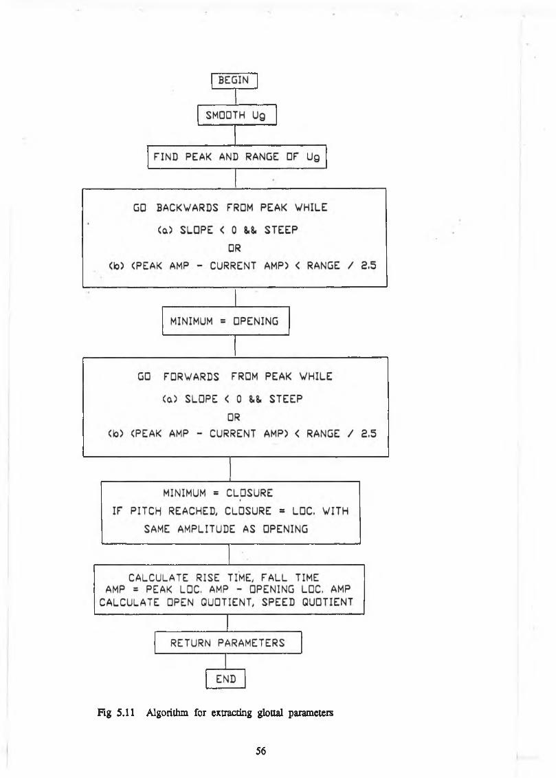


![7 Catheter-associated Urinary Tract Infection (CAUTI) · UTI Urinary Tract Infection (Catheter-Associated Urinary Tract Infection [CAUTI] and Non-Catheter-Associated Urinary Tract](https://static.documents.pub/doc/80x56/5c40b88393f3c338af353b7f/7-catheter-associated-urinary-tract-infection-cauti-uti-urinary-tract-infection.jpg)


