Water 2014, 6, 271-300; doi:10.3390/w6020271

water ISSN 2073-4441

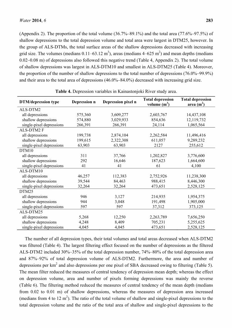
www.mdpi.com/journal/water

Article

Nationwide Digital Terrain Models for Topographic Depression Modelling in Detection of Flood Detention Areas

Jenni-Mari Vesakoski 1,*, Petteri Alho 1,2, Juha Hyyppä 3, Markus Holopainen 4,

Claude Flener 1 and Hannu Hyyppä 2,5

1 Department of Geography and Geology, University of Turku, Turku FI-20014, Finland;

E-Mails: petteri.alho@utu.fi (P.A.); claude.flener@utu.fi (C.F.) 2 Department of Real Estate, Planning and Geoinformatics, School of Engineering, Aalto University,

Aalto FI-00076, Finland; E-Mail: hannu.hyyppa@aalto.fi 3 Department of Remote Sensing and Photogrammetry, Finnish Geodetic Institute, Masala FI-02431,

Finland; E-Mail: juha.hyyppa@fgi.fi 4 Department of Forest Sciences, University of Helsinki, Helsinki FI-00014, Finland;

E-Mail: markus.holopainen@helsinki.fi 5 Civil Engineering and Building Services, Helsinki Metropolia University of Applied Sciences,

Helsinki FI-00079, Finland

* Author to whom correspondence should be addressed; E-Mail: jmeves@utu.fi;

Tel.: +358-2-333-5669.

Received: 19 November 2013; in revised form: 15 January 2014 / Accepted: 22 January 2014 /

Published: 28 January 2014

Abstract: Topographic depressions have an important role in hydrological processes as

they affect the water balance and runoff response of a watershed. Nevertheless, research

has focused in detail neither on the effects of acquisition and processing methods nor on

the effects of resolution of nationwide grid digital terrain models (DTMs) on topographic

depressions or the hydrological impacts of depressions. Here, we quantify the variation of

hydrological depression variables between DTMs with different acquisition methods,

processing methods and grid sizes based on nationwide 25 m × 25 m and 10 m × 10 m

DTMs and 2 m × 2 m ALS-DTM in Finland. The variables considered are the mean depth

of the depression, the number of its pixels, and its area and volume. Shallow and

single-pixel depressions and the effect of mean filtering on ALS-DTM were also studied.

Quantitative methods and error models were employed. In our study, the depression

variables were dependent on the scale, area and acquisition method. When the depths of

depression pixels were compared with the most accurate DTM, the maximum errors were

OPEN ACCESS

Water 2014, 6 272

found to create the largest differences between DTMs and hence dominated the amount

and statistical distribution of the depth error. On the whole, the ability of a DTM to

accurately represent depressions varied uniquely according to each depression, although

DTMs also displayed certain typical characteristics. Thus, a DTM’s higher resolution is no

guarantee of a more accurate representation of topographic depressions, even though

acquisition and processing methods have an important bearing on the accuracy.

Keywords: ALS; DTM; nationwide DEM; grid size; topographic depression; flood detention

1. Introduction

Spatial information is widely used in fluvial applications, the potential of which is increasing owing

to technological advances in topographic data acquisition. Laser scanning in particular has enabled

more accurate data gathering with decreased horizontal and vertical error and better availability of

detailed spatial data. For example, airborne laser scanning (ALS) [1–5], ALS systems for bathymetric

measurements [6], fixed-position terrestrial laser scanning (TLS) and mobile laser scanning (MLS),

such as boat- and cart-based mobile mapping systems (BoMMS/CartMMS) [7,8], have shown new

potential in fluvial research.

The acquisition method [9–12] and data processing method, such as grid size resampling [13,14],

of the elevation dataset impact on the accuracy of represented terrain derivatives. Furthermore,

horizontal [10–16] and vertical accuracy [10,17], terrain relief [13], algorithms used for terrain

derivative delineation and data structure affect the accuracy of a digital terrain model (DTM) [10].

Grid DTMs, which store elevation values in a regular matrix of pixels, are commonly used in

hydrologic analyses. The resolution, acquisition method and processing methods of a grid mainly

determine its error as a level of accuracy. The effects of the acquisition method and grid size of a DTM

on hydrologically interesting terrain derivatives, such as river network and watershed representation,

slope and aspect, specific catchment areas and CTI-values (Compound Topographic Index), have been

studied [10–12,18]. Additionally, the impact of vertical errors of DTMs on terrain derivatives has been

examined [10,17] as well as the impact of DTMs on hydrologic modelling [15,16,19] and flood

simulation [3,14,18]. The suitability of a DTM for terrain analysis has also been examined. For example,

Oksanen [20] focused on developing a three-step framework for exploring the suitability of a DEM for

terrain analyses; visualisation tools for detecting morphological gross errors [21], exploratory spatial

analysis of DTM error [22] and DEM error propagation analysis [23,24]. The last-mentioned step

focused on the results of error propagation analysis of slope, aspect and drainage basin delineation.

Because topographic depressions have an important role in hydrological processes as they affect the

water balance and runoff response of a watershed [25], they are used in flood risk management.

Nevertheless, research has not focused in detail on the effects of acquisition and processing methods

and resolution of a grid DTM on topographic depressions or the hydrological impacts of depressions.

Few studies have considered the effect of DTM grid size resampling on geometric attributes of

depressions [25–27]. To be more precise, Zandbergen [26] resampled 6 m grid size laser scanning

based DTM, Abedini et al. [25] resampled 3 mm grid size laser scanning based DTMs covering

Water 2014, 6 273

15 runoff plots, and Yang and Chu [27] resampled 5 mm grid size small laboratory surfaces and field

plots based on laser scanning and also watershed surfaces based on 30 m USGS-DTMs (U.S.

Geological Survey). Special attention has been paid to the total volume of depressions [13,28–30].

Research has also been performed on the effects of DTM grid size and the effects of a grid matrix

placement in relation to terrain on spurious depressions in DTMs [31] and also the effects of DTM

vertical error on depressions [32]. Furthermore, the potential of high-resolution DTMs to represent

linear anthropogenic features, such as depressions, and the use of these for more accurate flow pattern

modelling in human modified landscapes [4] has been examined. Additionally, research concerning the

effects of depressions on hydrologic models [5], the effects of the terrain slope [33], the effects of

surface roughness [34,35] on depressions and also the impacts of grid size on hydrologic connectivity

has been performed.

There have been no studies, as far as the authors are aware, concerning the characteristics of

nationwide DTMs in topographic depression detection. Recently, many countries have conducted

nationwide ALS surveys, principally for DTM purposes (e.g., the Netherlands, Switzerland, Denmark,

Finland, Sweden, Austria, Germany and the USA). For example, Denmark produced a digital elevation

model in 2006 and 2007 with national average point accuracy of 5.9 cm and point density of 1.6 m [36],

and Sweden’s new national elevation model will be available by 2015 and will have 2 m grid spacing

with mean vertical error of 0.5 m or less [37]. The National Land Survey of Finland (NLS) began to

gather new ALS-DTM data in 2008 that are planned to cover the whole country by 2019 [38]. Initially,

the collection concentrated on flood-prone areas. After the scanning of spring 2013, the total coverage

was approximately 235,000 km2 [39]. Thus, there is a growing need for better knowledge of the

suitability of nationwide elevation datasets for different study fields. All in all, detailed comparison

between accessible nationwide ALS-DTMs with different grid sizes and DTMs that represent more

conventional acquisition methods, such as photogrammetric methods, is needed.

The objective of this study is to quantify the variation of hydrological depression variables between

nationwide DTMs with different acquisition methods, processing methods and grid sizes. Our

depression detection is based on nationwide 25 m × 25 m and 10 m × 10 m DTMs and 2 m × 2 m

ALS-DTM produced by NLS of Finland. The depression variables considered are the mean depth of the

depression, the number of its pixels, and its area and volume. Furthermore, shallow and single-pixel

depressions are examined and also the effect of mean filtering on high-resolution ALS-DTM. The

results are compared with both field reference VRS-GNSS data (Virtual Reference Stations, Global

Navigation Satellite Systems) and the most accurate DTM verified with the aforementioned field

reference. Moreover, the differences of depression pixel depths in relation to the most accurate DTM

are determined and the effect of resolution on the detention areas for flooding is evaluated.

2. Background

Topographic depressions are part of a large framework of flood protection to control water

movement in a specific time scale (Figure 1). These effects cause changes in the shape and size of

hydrographs, runoff volume and time [5,25,40]. Thus, the aforementioned influences are brought about

by changes in water detention and direct surface runoff and are mainly achieved by adding, storing and

restoring detention and absorption areas for water on a watershed scale.

Water 2014, 6 274

Figure 1. Topographic depressions in the field (left) and in a grid digital terrain model

(DTM) (middle and right). Depressions can be simple or complex. Simple depressions

have one pour point (PP) and complex ones have more than one pour point of which one is

the actual pour point (APP) and the others are shared pour points (SPP) [40].

Topographic depression is defined as local minima of elevation values that have no downslope flow

paths [41] (Figure 1). Consequently, depressions are removed from a grid DTM prior to hydrologic

analyses that are based on automated simulation of surface runoff [41–43]. These analyses require

hydrologically connected flow networks, in which the flow to the actual pour point of the watershed is

not prevented.

There are two main conventions in depression preprocessing [44]. In the first one, depressions in

DTMs are real landscape features, and thus, methods do not modify them. According to the second

convention, depressions are spurious features caused by errors in DTM. These can be divided into

methods that process the whole DTM and methods that process only the problematic areas. These

methods that process only specific areas are commonly used in hydrology, and comprise filling,

breaching and combination methods (Figure 2) [42]. For example, Jenson and Domingue [41]

developed a filling method that is now implemented widely in commercial software products [1],

whereas several studies [1,45,46] have developed filling methods that are more suitable for large data

processing than the aforementioned method. A breaching method known as the phenomenon-based

approach, in which main flow paths are formed, was developed by Rieger [47]. These flow paths form

continuous paths from the deepest part of a depression to the actual pour point of the area studied

(Figure 2). A combination method called the Impact Reduction Approach (IRA) was developed by

Lindsay and Creed [48]. This method selects either the filling or the breaching method based on the

impact factor (IF) that indicates the amount of change in a DTM necessary for hydrologic correction of

the area processed. The method requiring the smallest change is chosen.

Water 2014, 6 275

Figure 2. Main principles of depression preprocessing methods. Depressions are caused by

underestimation of elevation values following filling methods that raise elevation values of

depression pixels. With the breaching methods, however, depressions are caused by

overestimation of elevation values which form topographic features that block water flow.

Depressions in a DTM are a combination of spurious and real terrain features. The separation of

these depression types is essential because of the impacts of real topographic depressions on

environmental processes such as watershed hydrology [49]. The development of a depression classifier

as a selective removal method is emphasised in low and smooth terrain, when accurate ALS-models

are used in which vertical error is near to the elevation differences of neighbouring pixels [26] or when

DTMs are used whose grid sizes are too large for detailed topography representation [31]. The

availability of more accurate DTMs that contain large amounts of depressions owed to LiDAR (Light

Detection and Ranging) technology also underlines the need for a classifier. For example, Liu and

Wang [2] classified modelled depressions from high-resolution ALS-DTM based on their spatial

variables. Zandbergen [32] focused on the effects of vertical accuracies of DTMs on the probability of

modelled depressions being actual landscape features. Lindsay and Creed [49] represented five

approaches for distinguishing real and spurious depressions from DTMs: ground inspection,

examination of source data, classification, and knowledge-based and modelling approaches.

3. Study Areas

Our study areas are the Lehmäjoki River (166 km2), the Nenättömänluoma River (107 km2) and the

upper reaches of the Kainastonjoki River (87 km2) whose watersheds are sub-basin areas (SBAs) of the

Kyrönjoki River watershed (Figure 3). The Kyrönjoki River watershed is located in the western part of

Finland and its main river bed drains into the Gulf of Bothnia. It mainly drains on a relatively flat

terrain, if the slopes of the three main tributaries of the Jalasjoki, Kauhajoki and Seinäjoki Rivers are

greater than the very gentle slopes of the main river bed [50]. The catchment area is 4923 km2 in size

and the proportion of lakes is small (1.23%). The principles of flood risk management were applied

to this flood-prone watershed in the 1960s. Consequently, extensive flood protection initiatives

(1966–2004) were executed. Also, flood risks have been evaluated and the significant flood risk areas

are listed by the Ministry of Agriculture and Forestry [51]. Two of these are situated in the Kyrönjoki

River watershed.

In this study, the watersheds were delineated by using techniques that involve the integration of a

specified vector hydrography layer [52], in which the stream network produced by the Finnish

Environment Institute was used. This stream network was added to the DTM by subtracting elevation

values of the river network from the unprocessed DTM. Thus, the pixels of the river network were

lowered. The flow directions, flow accumulation values, pour points and watersheds were delineated to

this processed DTM; additionally, the unprocessed DTM was cut by a watershed polygon.

Water 2014, 6 276

Figure 3. The watershed of Kyrönjoki River and the SBAs studied.

4. Materials and Methods

4.1. Field Survey Data

Field data were collected to provide reference data for the accuracy delineation of the DTMs. We

gathered 10,022 reference points from depressions in the Lehmäjoki River SBA with VRS-GNSS with

average horizontal standard deviation of 0.023 m and average vertical standard deviation of 0.04 m.

The satisfactory measure of DOP-value (Dilution of Precision) as PDOP-value (Position Dilution of

Precision) of gathered points was set at ≤5. PDOP is a figure that expresses the relationship between

the error of GPS position and the error of satellite position. Thus, it illustrates the positional

measurement accuracy and the smaller the value the more accurate the point gathered.

4.2. Laser Scanning Data

Recently, several countries have performed nationwide ALS surveys primary for DTM purposes.

In our study, ALS-DTM with 2 m grid size was used (Figure 4). This DTM is based on the ALS

point cloud that covers terrain with at least 0.5 points per 1 m2 (later ALS-DTM2) with accuracy

of 0.3 m [53,54]. The vertical point accuracy of the DTM is 0.15 m and horizontal accuracy is 0.6 m in

an unambiguous terrain surface. The ground points were selected from the point cloud and checked

Water 2014, 6 277

with TerraScan software and Espa environment [54,55]. The water bodies added were based on the

borderlines of topographic database (NLS) and the water heights were based on the average water

heights at the time of scanning. The checked ground points were interpolated by Lagrange’s method

and visualised. The vertical accuracy of ALS-DTM2 is approximately 0.3 m [53].

4.3. Conventional Nationwide DTMs

Nationwide 25 m × 25 m and 10 m × 10 m grid DTMs (later DTM10 and DTM25) produced by

NLS of Finland were used in this study (Figure 4). The elevation values of DTM25 are based on the

elevation data and water elements of the topographic database; in other words, on digitised and

interpolated contour lines of base maps of the 1990s. The vertical accuracy of DTM25 is 1.76 m

referenced to the national reference points of elevation [55,56]. DTM10 has been produced since

2001 along with the update and maintenance of the topographic database. In the aforementioned

updating process, water heights and shorelines, heights digitized in stereo workstations, heights of

water elements and other known elevation heights are added and data points of contour lines are

checked [55,56]. The vertical error of DTM10 is 1.4 m (95% of cases and 2 m 99% of cases) [57].

Figure 4. DTMs used in this study. (a) Pairs and groups of DTMs; (b) DTMs were

processed before analysis with the filling algorithm and the original DTMs were subtracted

from the processed DTMs. In this process, the depression pixels and their depths were

delineated. The depression pixels were selected and converted to polygons, for which the

depression variables were computed based on the processed DTMs.

4.4. Input Data Processing

In this study, ALS-DTM2 was resampled to 10 m × 10 m and 25 m × 25 m DTMs (later

ALS-DTM10 and ALS-DTM25) by using nearest-neighbour method. This method is commonly applied

in studies that concentrate on the impacts of different grid sizes of DTMs on terrain variables [26].

Method delineates new elevation values to output data without changing input elevations in any other

way. The changes in elevation values results from the resolution changes made. Thus, it was possible

to compare DTMs that represent the same grid size but different acquisition and processing methods.

Furthermore, the idea was to find alternatives to the high-resolution DTMs used in studies that require

high accuracy with DTMs that are faster to process. In our study, it was stated that the high-resolution

DTMs are used instead of DTMs with smaller representative accuracy but the same grid and data sizes

because of the growing availability of high-resolution ALS-DTMs. Furthermore, the ALS-DTM2 was

Water 2014, 6 278

filtered with mean filter (later ALS-DTM2 F) to delineate whether the representation of depressions

changed essentially from a flood risk perspective and if the number of small-in-volume depressions

and data sizes decreased. Consequently, this study was based on two elevation model groups and three

pairs of DTMs (Figure 4). Nevertheless, all DTMs were studied crosswise in statistical methods and

some tables and figures summarise all DTMs studied.

DTMs were processed with the depression filling algorithm developed by Wang and Liu [1]

(Table 1). This algorithm processes the grid from the edge areas to the inner parts by using the

least-cost search technique and raising the original elevation of a pixel (Elevation(n)) to its spill

elevation (Spill(c)) when needed. Spill elevation is the smallest elevation value to which the elevation

value of processed pixel needs to be raised in order for water to flow from the processed pixel to the

actual pour point of a grid. The pixel processing order is based on least-cost search-algorithm, which

selects the direction of propagation based on the smallest spill elevation value. Thus, the

depression-less flow path follows the spill elevations which become smaller towards the lower reaches.

The algorithm was chosen because of its small memory requirements and time complexity for large

high-resolution ALS-DTMs. A selection between filling algorithms was not essential because of the

parallel results among available filling algorithms, as also mentioned by Dhun [4].

Table 1. Pseudo-code for Wang and Liu algorithm [1].

Line Code

1 For b ← [cells on data boundary] 2 Spill[b] ← Elevation[b] 3 OPEN.push(Spill[b]) 4 While OPEN is not empty 5 c ← OPEN.top() 6 OPEN.pop(c) 7 CLOSED[c] ← true 8 For n ← [neighbours of c] 9 If n ϵ OPEN or CLOSED[n] = true

10 Then [do nothing] 11 Else 12 Spill[n] ← Max(Elevation[n], Spill[c]) 13 OPEN.push(n)

Notes: The spill elevation values are delineated starting from the lowest elevation pixel in the border of the

elevation data. A priority queue is declared as OPEN and it includes row number, column number and spill

elevation variables. The priority queue OPEN includes OPEN.push(), OPEN.top() and OPEN.pop() functions.

Function .push adds new nodes to the queue, .top finds the least-cost nodes and .pop removes least-cost nodes

from the queue. The array is declared as CLOSED and it marks the pixels that are processed as the central

pixels and removed from the OPEN queue.

4.5. Statistical Methods

The variation of depression variables in DTMs was examined both within and between SBAs using

descriptive statistics and statistical techniques. Descriptive statistics were mean, median and mode as

measures of central tendency, and standard deviation, minimum, maximum and percentiles as

Water 2014, 6 279

measures of dispersion. The statistical techniques were parametric Levene’s test and independent

samples t-test, and also nonparametric Kolmogorov-Smirnov test, Mann-Whitney U test and

Kruskal-Wallis test. The variables considered were mean depth of depression, and its number of pixels,

area and volume.

The research between SBAs focused on finding reasons for region dependency of depression

variables, while the research within SBAs was based on scale and acquisition method dependency. In

this study, parametric and non-parametric statistical techniques were used in parallel, as the fulfilment

of the assumptions of the parametric tests varied. In cases in which the aforementioned results differed,

the most probable result was considered.

4.6. Error Models

The elevation differences between gathered field reference data and DTMs were discovered by

digital elevation models of difference (DoD). These were made by subtracting elevation values of

DTMs from the elevation values of reference data points by using corresponding elevation values from

DTMs. Minimum, maximum and mean errors, standard deviations and root mean squared errors

(RMSEs) were calculated to describe the accuracy of DTMs in representing depressions. We also

applied the Nash-Sutcliffe model efficiency coefficient (NSE) to the predictive accuracy of a DTM

performance compared with field reference data (Equation (1)): = 1 − ∑ , ,∑ , (1)

where , is the ith surveyed elevation; , is the ith modelled elevation; is the mean surveyed

elevation; and n is the total number of observations [58,59]. NSE ranges between −∞ and 1.0, in which

NSEs from 0.0 to 1.0 are acceptable levels of performance, NSE 1.0 is the optimum and NSE < 0.0

means unacceptable performance in which the mean value of surveyed data is a better predictor than

the simulated values. It has been applied in hydrologic and hydraulic simulations [58,59], but it has

also been used to describe the predictive accuracy of other models, like suspended sediment and

morphodynamic models [60,61].

After the above-mentioned statistics were established, the depths of depression pixels were

compared with the most accurate DTM with error models in which depth errors were examined as

matrix of absolute values. The error values were calculated by subtracting depression pixel values of

DTMs studied and converting errors to absolute values. The dispersions of these error values, the

maximum and mean errors, standard deviations and surface area of error in SBAs were delineated.

4.7. Detention Area Survey

The threshold value for depression volume was delineated to 6000 m3 based on the example

presented in the general plan for flood risk management of the municipality of Ilmajoki (Figure 3) [62].

Preconditions were also set for the location, according to which the depressions located on acceptable

land use classes and at a range of 500 m from the stream channel were accepted. The selection between

land use classes was based on CORINE Land Cover, in which all but artificial areas were accepted.

Water 2014, 6 280

This survey was performed on depressions from which the river network was cut off. On the whole,

the detention area survey performed exemplified the spatial distribution of the error within SBAs.

5. Results

5.1. Accuracy Assessment of Depressions in DTMs Used

In our study, ALS-DTM2 was the most accurate DTM compared with reference data with RMSEs

ranging from 0.176 to 0.406 m (Table 2). R2 values of fitted linear regression lines of scatter plots

representing field reference elevations versus DTM elevations ranged from 0.947 to 0.982 and NSEs

ranged from 0.933 to 0.982 (Tables 2 and 3, Figure 5). ALS-DTM2 F was the next most accurate and

DTM25 was the least accurate DTM. NSEs of DTM25 are viewed as unacceptable performance [59].

DTM10 and ALS-DTM25 also had large RMSE values (0.728–1.698 m), unacceptable NSE values

((−0.844)–0.48) and R2 values ranged from 0.100 to 0.670. Only ALS-DTM2, ALS-DTM2 F and

ALS-DTM10 had NSEs that were considered as acceptable; in addition, ALS-DTM25 in reference

area G had an acceptable performance value of 0.51. The absolute mean errors were also calculated in

order to delineate the mean amount of the depth error (Table 2).

Figure 5. Scatter plots of reference data versus DTM elevations in reference area B.

(a) ALSDTM2; (b) ALS-DTM2 F; (c) ALS-DTM10; (d) DTM10; (e) ALS-DTM25;

(f) DTM25.

Water 2014, 6 281

Table 2. Difference between reference data and DTMs. N is the number of reference points in the reference area.

DTM Area N Minimum

dz (m) Maximum

dz (m) Absolute mean

error (m) RMSE (m) NSE

ALS-DTM2 A 2355 −2.27 4.097 0.230 0.406 0.958 ALS-DTM2 F A 2355 −2.29 4.279 0.249 0.426 0.951

DTM10 A 2355 −4.32 3.599 0.949 1.183 0.480 ALS-DTM10 A 2355 −3.90 4.029 0.521 0.839 0.816

DTM25 A 2355 −6.62 3.345 2.641 3.318 −0.594 ALS-DTM25 A 2355 −5.69 5.259 0.998 1.601 0.375 ALS-DTM2 B 2836 −1.03 1.132 0.184 0.214 0.949

ALS-DTM2 F B 2836 −1.01 1.313 0.200 0.243 0.927 DTM10 B 2836 0.00 1.408 0.540 0.728 0.130

ALS-DTM10 B 2836 −2.42 2.309 0.337 0.528 0.684 DTM25 B 2836 −3.76 1.557 1.261 1.538 −0.556

ALS-DTM25 B 2836 −2.74 2.207 0.595 0.918 0.058 ALS-DTM2 C 731 −2.22 1.298 0.238 0.321 0.966

ALS-DTM2 F C 731 −2.08 1.428 0.265 0.352 0.954 DTM10 C 731 −4.73 2.103 1.040 1.492 −0.574

ALS-DTM10 C 731 −3.37 3.349 0.609 0.899 0.710 DTM25 C 731 −5.41 1.472 1.802 2.493 −0.999

ALS-DTM25 C 731 −5.27 4.175 1.093 1.594 0.202 ALS-DTM2 D 578 −2.77 1.045 0.259 0.391 0.933

ALS-DTM2 F D 578 −2.51 1.317 0.326 0.464 0.896 DTM10 D 578 −3.13 1.549 1.484 1.698 −0.368

ALS-DTM10 D 578 −3.83 2.697 0.731 1.161 0.459 DTM25 D 578 −3.65 1.895 2.038 2.369 −0.679

ALS-DTM25 D 578 −3.73 3.656 1.196 1.643 −0.202 ALS-DTM2 E 922 −1.81 0.825 0.174 0.324 0.954

ALS-DTM2 F E 922 −1.73 1.071 0.214 0.357 0.939 DTM10 E 922 −2.89 4.380 1.000 1.290 −0.052

ALS-DTM10 E 922 −3.17 2.533 0.428 0.741 0.749 DTM25 E 922 −3.86 1.935 1.456 1.923 −1.866

ALS-DTM25 E 922 −3.37 4.793 1.224 1.606 −0.844 ALS-DTM2 F 865 −1.57 5.656 0.134 0.294 0.977

ALS-DTM2 F F 865 −1.56 5.618 0.160 0.323 0.971 DTM10 F 865 −1.92 5.734 1.121 1.368 −0.825

ALS-DTM10 F 865 −3.09 5.678 0.349 0.585 0.906 DTM25 F 865 −5.54 4.867 2.434 3.091 −0.734

ALS-DTM25 F 865 −4.87 5.362 0.810 1.311 0.510 ALS-DTM2 G 1734 −0.98 2.234 0.104 0.176 0.982

ALS-DTM2 F G 1734 −1.06 2.151 0.123 0.202 0.976 DTM10 G 1734 −3.58 3.776 1.018 1.271 0.203

ALS-DTM10 G 1734 −2.79 2.735 0.307 0.543 0.851 DTM25 G 1734 −5.03 1.519 3.904 4.115 −0.161

ALS-DTM25 G 1734 −4.35 4.078 0.768 1.250 0.305

Water 2014, 6 282

Table 3. R2 values of fitted regression lines of scatter plots representing DTM elevations

versus reference elevations. Scatter plots with fitted linear regression lines were used for

the Nash-Sutcliffe model efficiency coefficient (NSE) evaluation, as recommended

by [63–65], because of the high extreme values that could affect the NSE because of the

squared differences.

DTM/Area A B C D E F G ALS-DTM2 0.9633 0.9810 0.9782 0.9468 0.9594 0.9776 0.9824

ALS-DTM2 F 0.9590 0.9665 0.9723 0.9327 0.9503 0.9733 0.9773 DTM10 0.6697 0.5516 0.4137 0.5587 0.3337 0.5929 0.3709

ALS-DTM10 0.8326 0.7229 0.7429 0.5506 0.7755 0.9111 0.8532 DTM25 0.0091 0.0015 0.0030 0.0273 0.0073 0.0005 0.0053

ALS-DTM25 0.4717 0.2712 0.3520 0.1636 0.0995 0.6060 0.3835

5.2. Depression Variables in DTMs Studied

The total area of depressions, total number of depression pixels, area of depressions per km2 and

depression area in relation to the total surface area of SBA decreased with increasing grid size in both

DTM groups (Tables 4 and 5). In the group of NLS grid DTMs, the number of depressions was the

smallest in DTM10 and the largest in ALS-DTM2. Thus, depressions per km2 and number of

depressions per one pixel of SBA were smallest in DTM10. In the group of ALS-DTMs, the amount of

depressions per one pixel of SBA increased owing to resampling process, whereas the number of

depressions decreased with increasing grid size.

There were a large number of small depressions in terms of both area and volume in DTMs studied.

Depressions were the deepest in DTM25 and ALS-DTM25 (Table 6). Median and mode of depression

volume were also the largest in DTM25 in the group of NLS grid DTMs, whereas volume, area and

mean depth of depressions were the smallest and the shallowest in ALS-DTM2 (Table 6). Conversely,

the measures of the central tendency of the depression area and the pixel number in a depression were

largest in DTM10. In the group of ALS-DTMs, the mean depths (medians 0.02–0.12 m), volumes

(medians 0.11–91.25 m3) and areas (medians 4–625 m2) of depressions increased with grid size.

Single-pixel depressions were predominant in DTMs studied. The relative number of these mainly

increased with grid size (46.3%–79.8%), whereas the absolute number of single-pixel depressions

mainly decreased in both DTM groups with increasing grid size (Table 4). Yet, single-pixel depressions

were small in volume, the ratio of the total volume of single-pixel depressions to the total volume of

depressions increased (0.4%–22.3%) mainly with grid size in the group of ALS-DTMs (Appendix 1).

In the group of NLS grid DTMs, the DTM10 departed from the aforementioned trends with a relatively

small number of single-pixel depressions (10.6%–17.9%) and their volumes (0.002%–0.02%).

Shallow depressions (mean depth ≤0.3 m) were great in number. The absolute number of shallow

depression pixels decreased with increasing grid size in both DTM groups (Table 4). Furthermore, the

mean depth (medians 0.02–0.10 m) and median volume (0.11–63.12 m3) of depressions increased with

grid size (Appendix 2). In the group of NLS grid DTMs, the absolute number of shallow depressions

was smallest in DTM10 (Table 4). Furthermore, the ratio of the number of shallow depressions to the

total number of depressions (92.3%–93.9%) and their area to the total depression area (44.1%–57.5%)

was smallest in DTM10. These depressions were nevertheless largest in area (medians 750–1500 m2)

Water 2014, 6 283

(Appendix 2). The proportion of the total volume (36.7%–89.1%) and the total area (77.6%–97.5%) of

shallow depressions to the total depression volume and total area were largest in DTM25, however. In

the group of ALS-DTMs, the total surface areas of the shallow depressions decreased with increasing

grid size. The volumes (medians 0.11–63.12 m3), areas (medians 4–625 m2) and mean depths (medians

0.02–0.08 m) of depressions also followed this negative trend (Table 4, Appendix 2). The total volume

of shallow depressions was largest in ALS-DTM10 and smallest in ALS-DTM25 (Table 4). Moreover,

the proportion of the number of shallow depressions to the total number of depressions (76.0%–99.9%)

and their area to the total area of depressions (46.0%–84.0%) decreased with increasing grid size.

Table 4. Depression variables in Kainastonjoki River study area.

DTM/depression type Depression n Depression pixel n Total depression

volume (m3) Total depression

area (m2) ALS-DTM2

all depressions 575,360 3,609,277 2,603,767 14,437,108 shallow depressions 574,880 3,029,933 854,636 12,119,732 single-pixel depressions 266,391 266,391 24,114 1,065,564

ALS-DTM2 F all depressions 199,738 2,874,104 2,262,584 11,496,416 shallow depressions 199,615 2,322,308 611,057 9,289,232 single-pixel depressions 63,903 63,903 2127 255,612

DTM10 all depressions 311 37,766 1,202,827 3,776,600 shallow depressions 292 16,646 187,623 1,664,600 single-pixel depressions 41 41 61 4,100

ALS-DTM10 all depressions 46,257 112,383 2,752,926 11,238,300 shallow depressions 39,544 84,463 988,415 8,446,300 single-pixel depressions 32,264 32,264 473,651 2,528,125

DTM25 all depressions 946 3,127 214,935 1,954,375 shallow depressions 944 3,048 191,498 1,905,000 single-pixel depressions 597 597 37,312 373,125

ALS-DTM25 all depressions 5,268 12,250 2,263,789 7,656,250 shallow depressions 4,248 8,409 705,231 5,255,625 single-pixel depressions 4,045 4,045 473,651 2,528,125

The number of all depression types, their total volumes and total areas decreased when ALS-DTM2

was filtered (Table 4). The largest filtering effect focused on the number of depressions as the filtered

ALS-DTM2 included 30%–35% of the total depression number, 74%–80% of the total depression area

and 87%–92% of total depression volume of ALS-DTM2. Furthermore, the area and number of

depressions per km2 and also depressions per one pixel of SBA decreased owing to filtering (Table 5).

The mean filter reduced the measures of central tendency of depression mean depth; whereas the effect

on depression volume, area and number of pixels forming depressions was mainly the reverse

(Table 6). The filtering method reduced the measures of central tendency of the mean depth (medians

from 0.02 to 0.01 m) of shallow depressions, whereas the measures of depression area increased

(medians from 4 to 12 m2). The ratio of the total volume of shallow and single-pixel depressions to the

total depression volume and the ratio of the total area of shallow and single-pixel depressions to the

Water 2014, 6 284

total area of depressions decreased owing to filtering (Table 4). Additionally, mean filter decreased the

mean depths of single-pixel depressions (medians from 0.01 to 0.004 m), and thus the measures of

central tendency of volumes decreased (medians from 0.05 to 0.02 m3) (Appendix 1).

The number of all depression types, depression number per km2, depression area per km2, depression

area in relation to the total surface area of SBA and depressions per one pixel of SBA were mainly larger

in ALS-DTM10 than in DTM10 (Tables 4 and 5). Depressions were also deeper, in regards to measures

of central tendency, in ALS-DTM10 (means 0.14–0.17 m) than in DTM10 (means 0.06–0.11 m), whereas

DTM10 represented depressions larger in volume and area than ALS-DTM10 (Table 6). The total area

and volume of shallow and single-pixel depressions were mainly larger in ALS-DTM10 than in DTM10

(Table 4). Furthermore, the proportion of the total volume of the single-pixel and shallow depressions to

the total volume of all depressions and also the proportion of the total area of aforementioned depressions

to the total area of all depressions were mainly larger in ALS-DTM10 (17%–36%; 65%–75%) than in

DTM10 (16%–21%; 44%–58%) (Table 4). The shallow depressions in the ALS-DTM10 were smaller in

area (medians 100 m3) and volume (medians 7–9 m3) than in DTM10 (medians 750–1500 m2; 30–41 m3)

(Appendix 2). Single-pixel depressions were deeper in ALS-DTM10 (medians 0.05–0.08 m) and larger

in volume (medians 5.2–7.8 m3), than in DTM10 (medians 0.003–0.1 m; 0.3–1 m3) (Appendix 1).

The ALS-DTM25 included a larger number of all depression types studied than DTM25; in addition,

the total number of depression pixels, total volumes and areas of depressions were larger (Table 4).

The number and area of depressions per km2 were also larger in ALS-DTM25 than in DTM25 (Table 5).

Also, depression area in relation to the total surface area of SBA (5.8%–13.8%) and the number of

depressions per one pixel of the studied watershed (0.03–0.04/km2) were larger in ALS-DTM25 than

in DTM25 (2.3%–8.3%; 0.007–0.02/km2) (Table 5). The differences between DTM25 and

ALS-DTM25 depression variables were small (Table 6). In the ALS-DTM25, the depressions were

mainly larger, regarding their mean and median depth (medians 0.1 m) and volume (medians 81–91 m3),

than in DTM25 (0.1 m; 63 m3) when the standard deviations (SDEs), maximum values of variables

and percentiles were taken into account. Furthermore, mean depth, pixel number in a depression,

volume and area of shallow depressions were parallel, although the depressions were slightly larger in

volume, area and mean depth in DTM25 (Appendix 2). The total volume and area of the single-pixel

depressions were larger in ALS-DTM25 than in DTM25 (Appendix 1). Additionally, the relative

number of single-pixel depressions to the total area and volume of all depressions were larger in

ALS-DTM25 (17%–41%; 8%–22%) than in DTM25 (16%–27%; 7%–17%). The studied depression

variables of single-pixel depressions were parallel in DTM25 and ALS-DTM25 when the standard

deviations were taken into account.

Table 5. Distribution of depressions in Kainastonjoki River study area.

DTM Depression area/km2 Depressions/km2 % depression area of SBA

Depressions/one pixel of SBA

ALS-DTM2 166,422 6,632 16.6 0.0265 ALS-DTM2 F 132,249 2,298 13.2 0.0092

DTM10 43,534 4 4.4 0.0004 ALS-DTM10 129,548 533 13.0 0.0533

DTM25 22,531 11 2.3 0.0068 ALS-DTM25 88,256 61 8.8 0.0380

Water 2014, 6 285

Table 6. Statistical variables of all depressions in the Lehmäjoki River SBA;

(a) ALS-DTM2 and ALS-DTM2 F; (b) DTM10 and ALS-DTM10; and (c) DTM25 and

ALS-DTM25.

(a)

ALS-DTM2 ALS-DTM2 F

Pixels/

depression

Mean

depth (m)

Volume

(m3) Area (m2)

Pixels/

depression

Mean

depth (m)

Volume

(m3) Area (m2)

Mean 9.34 0.03 10.75 37.37 23.31 0.02 29.69 93.23

Median 2.00 0.02 0.13 8.00 3.00 0.01 0.13 12.00

Mode 1.000 0.002 0.008 4.000 1.000 0.001 0.004 4.000

SDE 772.02 0.04 2,330.56 3,088.07 1,363.55 0.03 4,071.90 5,454.19

Minimum 1.000 0.001 0.004 4.000 1.000 0.001 0.004 4.000

Maximum 493,837 3.72 1,662,117 1,975,348 497,226 3.72 1,667,566 1,988,904

Percentiles

25 1.000 0.008 0.040 4.000 1.000 0.005 0.031 4.000

75 4.00 0.04 0.46 16.00 8.00 0.02 0.64 32.00

(b)

DTM10 ALS-DTM10

Pixels/

depression

Mean

depth (m)

Volume

(m3) Area (m2)

Pixels/

depression

Mean

depth (m)

Volume

(m3) Area (m2)

Mean 57.49 0.11 2,604.54 5,748.826 3.63 0.14 119.19 363.02

Median 9.00 0.06 45.35 900.00 1.00 0.06 9.20 100.00

Mode 1.000 0.002 0.200 100.000 1.000 0.007 0.700 100.000

SDE 427.14 0.18 34,961.60 42,713.77 85.81 0.20 6,912.35 8,581.18

Minimum 1.000 0.001 0.100 100.000 1.000 0.001 0.100 100.000

Maximum 17,954 3.34 1,684,317 1,795,400 18,676 3.54 1,524,178 1,867,600

Percentiles

25 2.000 0.002 5.599 200.000 1.000 0.023 2.800 100.000

75 30.00 0.14 359.38 3,000 2.00 0.18 30.80 200.000

(c)

DTM25 ALS-DTM25

Pixels/

depression

Mean

depth (m)

Volume

(m3) Area (m2)

Pixels/

depression

Mean

depth (m)

Volume

(m3) Area (m2)

Mean 3.81 0.10 532.96 2,381.27 4.10 0.19 1,082.06 2,561.96

Median 1.00 0.10 62.50 625.00 1.00 0.10 80.63 625.00

Mode 1.000 0.100 62.499 625.000 1.000 0.004 2.500 a 625.000

SDE 41.64 0.03 13,499.30 26,024.013 52.94 0.26 23,446.43 33,090.2014

Minimum 1.000 0.100 62.500 625.000 1.000 0.001 0.625 625.000

Maximum 2,729 1.43 671,376 1,705,625 2,992 2.52 1,480,272 1,870,000

Percentiles

25 1.00 0.10 62.50 625.00 1.00 0.04 25.63 625.00

75 2.25 0.10 187.50 1,406.25 2.00 0.24 248.13 1,250.00

Note: a Variable has multiple modes, from which the smallest is represented in the table.

5.3. Statistical Methods

The statistical distributions of depression variables diverged between corresponding DTMs of SBAs.

This variation was statistically significant (p < 0.05) in the majority of variables (Tables 7 and 8).

,argest similarities were found in volumes of DTM10 and DTM25. Furthermore, the distribution of

Water 2014, 6 286

depression variables within SBA varied with grid size, acquisition method and processing method of a

grid DTM (p < 0.05) with some similarities.

Some particular statistical characteristics were found: (1) the distributions of depression variables

diverged statistically from ALS-DTM2 within areas. Thus, the statistical variation of depression

variables between ALS-DTM2 and ALS-DTM2 F was statistically significant (p < 0.001); (2) The

statistical distributions of depression variables differed (p < 0.001) between DTM10 and ALS-DTM10

within areas; (3) The amount of statistical similarity was greatest between DTM25 and ALS-DTM25.

Table 7. Kruskal-Wallis test results, when the similarities of distributions of the depression

variables were studied (a) within SBAs (b) between SBAs. The confidence level was set

to 95%. According to the results the difference of distributions are statistically significant

(p < 0.001), with some exceptions.

(a) Kauhajoki River upper

reaches Lehmäjoki River

watershed Nenättömänluoma River

watershed Pixel/depression p < 0.001 p < 0.001 p < 0.001

Volume of a depression p < 0.001 p < 0.001 p < 0.001 Area of a depression p < 0.001 p < 0.001 p < 0.001

Mean depth of a depression p < 0.001 p < 0.001 p < 0.001

(b) ALS-

DTM2 ALS-DTM2

F DTM10

ALS-DTM10

DTM25 ALS-

DTM25 Pixel/depression p < 0.001 p < 0.001 p < 0.001 p < 0.001 p < 0.001 p < 0.001

Volume of a depression p < 0.001 p < 0.001 p = 0.104 p < 0.001 p < 0.001 p = 0.082 Area of a depression p < 0.001 p < 0.001 p < 0.001 p < 0.001 p < 0.001 p < 0.001

Mean depth of a depression p < 0.001 p < 0.001 p < 0.001 p < 0.001 p < 0.001 p < 0.001

Table 8. The statistical similarity (X) and difference (*) of the distributions of depression

variables (a) between SBAs and (b) within SBAs, when the Kolmogorov-Smirnov test,

Levene’s test, independent samples t-test and Mann-Whitney U test were used (See notes).

(a) Trend

ALS-DTM2 ALS-DTM2 F DTM10 DTM25 ALS-DTM10 ALS-DTM25 Lehmäjoki River and Kainastonjoki River SBAs

Pixels/depression -/* -/*** -/*** -/X -/*** -/*** Volume */*** */*** X/*** X/*** */*** */X

Area ***/* **/*** */X X/*** ***/*** **/*** Mean depth ***/*** X/*** ***/*** X/*** ***/*** X/***

Kainastonjoki River and Nenättömänluoma River SBAs Pixels/depression -/*** -/*** -/X -/X -/*** -/***

Volume X/*** X/*** X/X X/* X/*** X/X Area X/*** X/*** X/X **/X X/*** X/***

Mean depth ***/*** X/*** **/* X/** ***/*** ***/** Lehmäjoki River and Nenättömänluoma River SBAs

Pixels/depression -/*** -/*** -/*** -/*** -/*** -/*** Volume X/*** X/*** X/X X/*** X/*** */*

Area ***/*** ***/*** **/*** */*** ***/*** ***/*** Mean depth ***/*** X/*** X/*** */*** ***/*** ***/***

Water 2014, 6 287

Table 8. Cont.

(b) Trend

ALS-DTM2 ALS-DTM2 F DTM10 DTM25 ALS-DTM10 ALS-DTM25 Depression volume (upper part) and area (lower part) in Kainastonjoki River

ALS-DTM2 X/*** **/*** ***/*** ***/*** ***/*** ALS-DTM2 F ***/*** **/*** ***/*** ***/*** ***/***

DTM10 ***/*** ***/*** **/*** **/*** */*** DTM25 ***/*** ***/*** ***/*** ***/*** ***/***

ALS-DTM10 ***/*** ***/*** ***/* ***/*** X/X ALS-DTM25 ***/*** ***/*** ***/*** ***/*** **/***

Depression mean depth (upper part) and pixels per depression (lower part) in Kainastonjoki River SBA ALS-DTM2 ***/*** ***/*** ***/*** ***/*** ***/***

ALS-DTM2 F -/*** ***/*** ***/*** ***/*** ***/*** DTM10 -/*** -/*** ***/*** ***/*** ***/X DTM25 -/*** -/*** -/*** ***/*** ***/***

ALS-DTM10 -/*** -/*** -/*** -/*** ***/*** ALS-DTM25 -/*** -/*** -/*** -/*** -/***

Depression volume (upper part) and area (lower part) in Lehmäjoki River SBA ALS-DTM2 */*** ***/*** ***/*** **/*** ***/***

ALS-DTM2 F ***/*** ***/*** **/*** **/*** ***/*** DTM10 ***/*** ***/*** ***/*** ***/*** */*** DTM25 ***/*** ***/*** ***/*** */*** ***/***

ALS-DTM10 ***/*** ***/*** ***/*** ***/*** X/*** ALS-DTM25 ***/*** ***/*** ***/X ***/*** X/*** Depression mean depth (upper part) and pixels per depression (lower part) in Lehmäjoki River SBA ALS-DTM2 ***/*** ***/*** ***/*** ***/*** ***/***

ALS-DTM2 F -/*** ***/*** ***/*** ***/*** ***/*** DTM10 -/*** -/*** ***/*** **/*** ***/*** DTM25 -/*** -/*** -/*** ***/*** ***/***

ALS-DTM10 -/*** -/*** -/*** -/*** ***/* ALS-DTM25 -/*** -/*** -/*** -/*** -/***

Depression volume (upper part) and area (lower part) in Nenättömänluoma River SBA ALS-DTM2 */*** **/*** ***/*** ***/*** ***/***

ALS-DTM2 F ***/*** **/*** ***/*** ***/*** ***/*** DTM10 ***/*** ***/*** **/*** **/*** **/X DTM25 ***/*** ***/*** ***/*** X/*** ***/***

ALS-DTM10 ***/*** ***/*** ***/*** ***/*** **/X ALS-DTM25 ***/*** ***/*** ***/*** ***/*** X/***

Depression mean depth (upper part) and pixels per depression (lower part) in Nenättömänluoma River SBA ALS-DTM2 ***/*** ***/*** ***/*** ***/*** ***/***

ALS-DTM2 F -/*** ***/*** ***/*** ***/*** ***/*** DTM10 -/*** -/*** ***/*** X/*** ***/*** DTM25 -/*** -/*** -/*** ***/*** ***/***

ALS-DTM10 -/*** -/*** -/*** -/*** ***/*** ALS-DTM25 -/*** -/*** -/*** -/X -/***

Notes: The pairs of DTMs represented by green backgrounds fulfilled the hypothesis of same variances; otherwise, pairs with a red background did not fulfil this hypothesis with 95% confidence value. Red fonts represent pairs that obeyed normal distribution after logarithmic transformation, although non-normal distributions can be dismissed based on central limit theorem in cases where the hypotheses of same variances were fulfilled. Thus, boxes with a red background are read from the right side of the backslash (non-parametric tests) and boxes with a green background are read from the left side (parametric tests). Pixels per depression represent the ordinal scale, and thus only the non-parametric tests were applied. Here *** represents statistically highly significant difference (p < 0.001); ** significant difference (p < 0.01); and * almost significant difference (p ≤ 0.05).

Water 2014, 6 288

5.4. Error Models

A substantial amount of depth error was small in relation to ALS-DTM2 as reference data and also

in relation to the vertical errors of the DTMs studied. Thus, the maximum values of errors represented

the largest differences between DTMs (Table 9, Figure 6). ALS-DTM10 and ALS-DTM25 had a

smaller maximum of errors than DTM10 and DTM25, whereas the filtered ALS-DTM2 had the

smallest maximum error values. The maximum errors of ALS-DTMs increased with grid size.

The surface area of studied SBA containing depth error improved the idea about the characteristics

of depth error in DTMs (Table 9). The relative proportions of the error surface area increased with

grid size in both DTM groups. The filtered ALS-DTM2 included the smallest error surface area

(14%–21%). ALS-DTM10 contained a smaller proportion of error area (36%–56%) than DTM10

(48%–63%), whereas the surface areas of error were parallel in DTM25 and ALS-DTM25.

Table 9. Depth error in relation to ALS-DTM2.

Area/DTM Maximum (m) Mean (m) SD (m) Median (m) Surface areas of error in SBAs (%) Kainastonjoki ALS-DTM2 F 2.07 0.007 0.03 0.023 19.1

DTM10 6.43 0.03 0.18 0.007 63.1 ALS-DTM10 2.69 0.03 0.09 0.002 35.9

DTM25 6.32 0.03 0.18 0.006 84.3 ALS-DTM25 3.33 0.03 0.10 0.007 84.4

Nenättömänluoma ALS-DTM2 F 2.05 0.005 0.04 0.019 13.5

DTM10 8.14 0.06 0.33 0.006 48.2 ALS-DTM10 3.89 0.02 0.11 0.006 47.1

DTM25 8.10 0.04 0.28 0.004 66.7 ALS-DTM25 5.44 0.04 0.19 0.005 66.8

Lehmäjoki ALS-DTM2 F 1.54 0.01 0.04 0.025 21.1

DTM10 5.03 0.07 0.22 0.011 59.1 ALS-DTM10 3.52 0.04 0.12 0.008 56.2

DTM25 5.44 0.06 0.24 0.008 77.7 ALS-DTM25 3.71 0.03 0.10 0.008 76.9

Figure 6. The distributions of depth error in (a) Kainastonjoki and (b) Nenättömänluoma

River SBAs. In ALS-DTMs, the surge of depth error occurred at higher percentage points

than in NLS grid DTMs.

Water 2014, 6 289

On the whole, the amount of depth error varied uniquely with depression. Figure 7 represents

typical characteristics of specific DTMs to describe depressions and also illustrates the formation of

depth error.

Figure 7. Terrain and depression representations of DTMs studied. An aerial photograph

acts as a background. The blue line illustrates the stream channel and red depressions;

when the tone gets darker the depression pixels are deeper.

Water 2014, 6 290

5.5. Survey of Detention Areas for Water

There were differences between locations, total numbers and total volumes of depressions that met

the criteria set in Section 4.7 (Figures 8 and 9). The total number of depressions ranged from 7 to 46 and

total volume ranged from 1.39 to 3.97 million m3 between DTMs studied. When the above-mentioned

depression variables were compared with the depressions represented in ALS-DTM2, both the DTM25

and ALS-DTM10 varied most from the reference data (Figures 8 and 9). Furthermore, the difference in

ALS-DTM2 F, DTM10 and ALS-DTM25 was the smallest.

When the DTMs were studied in more detail some observations were possible: (1) the difference

between filtered ALS-DTM and ALS-DTM2 was the smallest with 84% equivalence in total

depression number and 96% in total volumes. Filtered ALS-DTM2 was the only DTM that represented

all of the largest depressions represented in reference DTM; (2) The difference of depression variables

in relation to reference DTM was larger in ALS-DTM10 than in DTM10. ALS-DTM10 represented

only 39% of the total depression number and 50% of the total depression volume in relation to the

depressions in DTM10; (3) DTM25 differed more from the reference DTM than ALS-DTM25.

DTM25 represented 27% of the total depression number and 38% of the total depression volume in

relation to the depressions in ALS-DTM25; (4) ALS-DTM25 generalised the terrain representation of

ALS-DTM2 as expected, although the ALS-DTM10 was an intermediate form that was lacking some

of the information represented in ALS-DTM25.

Figure 8. The modelled detention areas for water: (a) number ;and (b) volumes of depressions

that met the set criteria; (c) maximum and (d) minimum volumes of depressions chosen.

Water 2014, 6 291

Figure 9. Locations and volume classes of depressions that met the set criteria.

6. Discussion

6.1. The Accuracy of DTMs for Representing Terrain

In our study, ALS-DTM2 was the most accurate DTM used in relation to reference data and also

was most successful in terms of terrain representation. ALS-DTMs represented terrain more accurately

than nationwide NLS grid DTMs, and also the accuracy of a DTM to represent terrain decreased with

increasing grid size in both DTM groups studied. This finding is supported by earlier studies [3,55,66]

which assert that the nationwide 25 m × 25 m and 10 m × 10 m NLS grid DTMs do not meet all the

modern requirements for representation accuracy. These findings are supported by Oksanen [20]

according to whom an increase in the DTM vertical error will increase the error in surface derivatives

such as slope, aspect and watershed delineation in fine toposcale elevation datasets that are typically

represented in a 5‒50 m grid and derived from contour data.

6.2. The Variation of the Hydrological Depression Variables

In our study, acquisition method, processing method and grid size of DTMs affected both the

location and the hydrological variables of depressions. Furthermore, the variables studied were

dependent on the scale and acquisition method of the DTM and also the area studied. This finding is

Water 2014, 6 292

supported by Chu et al. and colleagues [13,25–27] concerning the area and scale dependency of

depression variables. In our study, the depression variables also showed more regularity in the group of

ALS-DTMs in which DTMs based on the same acquisition method were resampled than in the group

of NLS grid DTMs based on different acquisition and processing methods. Similar results can be also

found in earlier studies [10,18].

The number of all depressions and depression pixels decreased with increasing grid size in the

group of ALS-DTMs. For example, Abedini et al. and colleagues [25–27,33] obtained parallel results

in relation to the depression number. In our study, both the shallow and the single-pixel depressions

also followed this negative trend in the group of ALS-DTMs. Furthermore, the number of depression

pixels followed the aforementioned negative trend in the group of NLS grid DTMs. These observed

regularities can mainly be explained by the accurate representation of terrain microtopography in the

high-resolution DTMs and the generalisation of this representation with growing grid size [1,26].

In addition, the number of pixels for a given area decreases by a power of two with increasing grid

size [31] and consequently explains our findings.

The total areas of depressions followed a decreasing trend with increasing grid size in both DTM

groups. This finding can be explained by the changes of both small-in-size and artificial depressions

with increasing grid size [26]. The occurrence of small depressions is substantial in high-resolution

DTMs. The absolute numbers of small depressions decreases with increasing grid size, because larger

grid sizes do not enable the representation of small depressions in the same way as DTMs with smaller

grid sizes. Additionally, the vertical accuracy of high-resolution DTM approaches the height difference

between neighbouring pixels, resulting in small depressions. This hypothesis needs to be separated

from the observation made in our study that DTM25 and ALS-DTM25 included the highest relative

numbers of single-pixel depressions. These findings can be partly explained by the squaring of

the pixel number with increasing grid size [31] and the fact that the grid size of a DTM affects

the accuracy of its terrain representation [26]. Thus, the results of our study parallel those of

Zandbergen [26], but diverge from those of Abedini et al. [25] and partly diverge from those of

Chu et al. [13] and also Yang and Chu [27]. According to Abedini et al. [25], the total areas of

depressions (%) follow an increasing trend with grid size in a group of laser scanning based DTMs.

According to Yang and Chu [27], the total areas of depressions followed decreasing trend with grid

size in laser scanning based laboratory and field plot surfaces. Whereas, resampled 30 m USGS-DEM

followed increasing trend with grid size. According to Chu et al. [13], depression area (m2) is

area-dependent. In our study, total areas of depressions varied between SBAs maintaining the

trends aforementioned.

In our study, the regional dependency of the depression total volumes was highlighted. This

variable did not follow any clear trend between SBAs. Our results are parallel with that of

Chu et al. [13], in that the regional dependency is influenced by the microtopography of the SBA and

also the acquisition method and grid size of the DTM. The results of our study were different from

those of earlier studies [25–28,67]. Only the volumes of nationwide NLS grid DTMs in Kainastonjoki

and Nenättömänluoma River SBAs followed the decreasing trend with increasing grid size presented

by earlier studies [26,28–30]. The generalisation of the terrain representation with increasing grid size

is mentioned as the main reason for this negative trend. Kamphorst [67] represents that the total

volume of depressions increases at first but is stabilised with increasing grid size.

Water 2014, 6 293

The mean filter did not change the representation of depressions or the values of depression

variables excessively, because in the flood risk management perspective, depressions which are small

in volume and separate are not the most essential. Furthermore, the data sizes decreased. Our finding

was expected, because the mean filter determines new elevation values based on the neighbouring

pixels of processed pixels. The mean filter generalised slightly the elevation values of DTMs. Thus,

different kinds of filters are used for reducing data noise and removing small depressions [41,43,68].

ALS-DTM10 and ALS-DTM25 were more accurate in relation to the reference data than

DTM10 and DTM25. This difference between NLS grid 10 and ALS-DTM10 is also mentioned by

Vilhomaa [55]. In our study, ALS-DTMs included a larger number of all studied depression types than

DTM10 and DTM25. Additionally, ALS-DTM10 and ALS-DTM25 included more depressions per

square kilometre and per one pixel of SBA. The depression area per square kilometre, relative amounts

of depressions from the total area of SBA and relative amounts of single-pixel depressions from all

depressions were generally also greater in ALS-DTMs than in DTM10 and DTM25. These results

were expected, because ALS-DTM2 represented the terrain microtopography accurately and the

generalisation of this due to the resampling process created separate but scattered depression pixels.

The difference between ALS-DTM25 and NLS grid DTM25 was the smallest and the difference

between ALS-DTM10 and DTM10 was the largest of all pairs studied. The number of depressions was

lowest in DTM10, but these depressions were largest in area.

6.3. Error Models and Detention Area Survey

The maximum depth errors in relation to ALS-DTM2 gave us a general idea about the differences

between DTMs in terms of representing depressions. Furthermore, error models and statistical

parameters illustrated some typical characteristics of specific DTMs for representing certain types of

depressions. The spatial distribution of errors and the impact of the depth errors on separate

depressions were not seen, however, until more detailed visual examinations were performed.

The results of the detention area survey supported the conclusions drawn from depth error models

and statistics, according to which the variables of depressions were acquisition method, processing

method and scale dependent. The varying accuracy of specific DTMs in terms of representing separate

depressions in relation to reference data was emphasised. This heterogeneous quality of nationwide

NLS grid DTMs is also mentioned by earlier studies [22,55]. It is caused by errors in photogrammetric

stereo interpretation which are in turn caused by systematic errors in contour data, the low accuracy of

terrain elevations, and coverage of terrain that causes difficulties in the interpretation of stereo images.

Problems can also arise with the aerial photography techniques available, large grid sizes, different

methods used to produce contour lines, problems updating contour lines and the algorithms used to

create the elevation datasets. The representation of low-lying and flat areas can be very erroneous

because of the generalised terrain representation [69]. In our study, the variation in accuracy was

limited by the statistical distribution of depression variables and the results of error models performed.

This distribution of error is best described by robust descriptors of distributions as quantiles and

maximums, in addition to conventional measures of distribution. This is also supported by Oksanen

and Sarjakoski [22].

Water 2014, 6 294

The results of the detention area survey were the same as those of depth error models in that

mean-filtered ALS-DTM2 was the closest to ALS-DTM2. The impact of filtering was particularly

evident in the depressions whose volume was near the threshold set. In contrast to error models,

DTM10 was closer to ALS-DTM2 than ALS-DTM10 in the detention area survey, whereas

ALS-DTM25 was closer to ALS-DTM2 than DTM25, as also shown in error models. The typical

ability of DTM10 to represent depressions as unbroken in shape and large in area in relation to other

DTMs explains the above-mentioned observations, whereas DTM25 represented the same as a group

of scattered pixels. Furthermore, the generalisation of ALS-DTM2 represented depressions with

varying degrees of success, depending on the depression examined.

7. Conclusions

Our study has demonstrated the effects of acquisition method, processing method and grid size of

nationwide DTMs on the detection of topographic depressions and their hydrological variables. This

was performed by using quantitative statistics, digital elevation models of difference and error models.

According to our study, the decision about the suitability of the available DTMs for a specific purpose

should be made based on the demands of the problem settings and accuracy. In future studies with a

relatively low demand for accuracy, awareness of the error, its level, and effects on analyses in general

is sufficient. In more accurate studies, the awareness of the varying spatial accuracy of a DTM in

representing terrain is emphasised. Furthermore, knowledge about certain typical characteristics of

available DTMs in representing a studied terrain variable or variables is essential. Field work also

needs to be considered. It is also recommended to use the most accurate DTM that computing

resources can process. Furthermore, the interpretation of results is recommended together with the

classification of variables under study (e.g., depth classification of depressions), as well as setting

thresholds for it (e.g., volumes of depressions considered).

Furthermore, the following specific conclusions can be drawn:

ALS-DTMs are closer to the real topography of depressions than DTMs based on more

conventional acquisition and processing methods. The accuracy of terrain representation

decreased with increasing grid size in both groups of DTMs.

The acquisition method, processing method and grid size of a DTM has an impact on modelled

depression variables. This variation was found to be area, acquisition method, processing method

and scale dependent.

• The difference between ALS-DTM10 and DTM10 is the largest. The principal reason was

the scattered depression pixels that were great in number because of the resampling process

performed. The number of these separate fragmental pixels decreased as the degree of

terrain representation became greater with increasing grid size. DTM10 also differed from

the other DTMs in terms of statistical significance.

• The absolute number of depressions and depression pixels is larger in ALS-DTM10 and

ALS-DTM25 than in DTM10 and DTM25. This is a consequence of the resampling process

of ALS-DTM2 that produces scattered depression pixels.

• The mean filtering of ALS-DTM2 focuses on the small and shallow depressions, and is thus

suitable for detection of water detention areas in flood risk management.

Water 2014, 6 295

The maximum pixel depth error of a DTM illustrated the amount of depth error in relation to

ALS-DTM2 in a most descriptive way. ALS-DTMs have smaller maximum error values than the

nationwide NLS grid DTMs 10 m × 10 m and 25 m × 25 m.

The accuracy of DTMs in representing separate depressions varied. Thus, the decreasing grid

size of a DTM is no guarantee of increasing spatial accuracy when there is a demand for the

most accurate data available. According to the aforementioned findings, the acquisition method,

processing method and grid size of a DTM have an impact on the location, number and total

volumes of depression areas.

Acknowledgments

Funding for this study (GIFLOOD, FLOODAWARE, LuhaGeoIT and RivCHANGE projects) was

supplied by the Finnish Funding Agency for Technology and Innovation (Tekes), the Maj and Tor

Nessling Foundation, the Ministry of Agriculture and Forestry and the Academy of Finland.

Conflicts of Interest

The authors declare no conflict of interest.

Appendix

Appendix 1. Variables for single-pixel depressions. The mean values are represented in

brackets because of the skewed distributions of depression variables.

Area/DTM Depression

number Median mean

depth (m) SD mean depth (m)

Median volume (m3)

SD volume (m3)

Max depth (m)

Upper reaches of Kainastonjoki River SBA ALS-DTM2 266,391 0.01 (0.02) 0.03 0.05 (0.09) 0.12 0.51

ALS-DTM2 F 63,903 0.005 (0.008) 0.01 0.02 (0.03) 0.04 0.19 DTM10 41 0.003 (0.01) 0.05 0.30 (1.49) 5.29 0.34 DTM25 597 0.10 (0.10) 0.000002 62.50 (62.50) 0.001 0.10

ALS-DTM10 32,264 0.08 (0.15) 0.19 7.80 (14.98) 18.91 2.74 ALS-DTM25 4045 0.10 (0.19) 0.25 64.38 (117.10) 156.08 4.51

Nenättömänluoma River SBA ALS-DTM2 266,830 0.01 (0.02) 0.03 0.04 (0.03) 0.12 0.47

ALS-DTM2 F 55,901 0.005 (0.009) 0.01 0.02 (0.01) 0.04 0.19 DTM10 50 0.004 (0.01) 0.02 0.40 (0.98) 2.25 0.15 DTM25 954 0.10 (0.10) 0.01 62.50 (62.83) 6.71 0.40

ALS-DTM10 29,459 0.07 (0.17) 0.22 7.50 (16.52) 22.12 2.43 ALS-DTM25 3619 0.11 (0.22) 0.30 68.75 (137.19) 186.96 3.72

Lehmäjoki River SBA ALS-DTM2 365,225 0.01 (0.02) 0.03 0.04 (0.54) 0.12 0.54

ALS-DTM2 F 76,014 0.004 (0.008) 0.01 0.02 (0.15) 0.04 0.15 DTM10 701 0.01 (0.02) 0.04 1.00 (2.29) 3.90 0.55 DTM25 3178 0.10 (0.10) 0.01 62.50 (62.18) 7.68 0.60

ALS-DTM10 40,073 0.05 (0.14) 0.21 5.20 (13.98) 21.05 2.37 ALS-DTM25 5854 0.08 (0.19) 0.26 52.50 (116.97) 160.63 2.42

Water 2014, 6 296

Appendix 2. Variables for shallow (mean depth ≤ 0.3 m) depressions. The mean values are

represented in brackets because of the skewed distributions of depression variables.

Area/DTM Depression

number

Depression

pixel

number

Median

mean

depth (m)

SD

mean

dept

h (m)

Median volume

(m3)

SD

volume

(m3)

Median area

(m2)

SD area

(m2)

Upper reaches of Kainastonjoki River SBA

ALS-DTM2 574,880 3,029,933 0.02 (0.03) 0.04 0.14 (1.49) 40.46 8.00 (21.08) 309.68

ALS-DTM2F 199,615 2,322,308 0.01 (0.02) 0.02 0.12 (3.06) 81.94 12.00 (46.54) 397.37

DTM10 292 16,646 0.03 (0.05) 0.06 29.50 (642.55) 2,357.1

6

1350

(5,700.68) 13,931.44

DTM25 944 3048 0.10 (0.10) 0.006 62.50 (202.86) 496.20 625 (2018) 4,869.32

ALS-DTM10 39,544 84,463 0.07 (0.09) 0.08 9.20 (25) 235.30 100 (213.59) 994.02

ALS-DTM25 4248 8409 0.08 (0.10) 0.08 63.12 (166.01) 1,179.6

8

625

(1,237.20) 5,150.54

Nenättömänluoma River SBA

ALS-DTM2 514,387 2,260,555 0.02 (0.03) 0.03 0.11 (1.08) 34.20 4.00 (17.58) 162.14

ALS-DTM2F 156,593 1,573,508 0.01 (0.02) 0.02 0.10 (2.34) 45.92 12.00 (40.19) 260.31

DTM10 434 31,456 0.03 (0.06) 0.07 40.80 (1,124.32) 4,052.1

2

1500

(7,247.93) 18,371.54

DTM25 1462 3077 0.10 (0.10) 0.004 62.50 (1,315.41) 234.39 625 (1,315.4) 2,253.94

ALS-DTM10 31,026 55,190 0.06 (0.08) 0.08 7.00 (18.33) 147.74 100 (177.88) 715.02

ALS-DTM25 3445 5278 0.08 (0.10) 0.08 55.63 (111.19) 383.61 625 (957.55) 1,784.74

Lehmäjoki River SBA

ALS-DTM2 777,433 4,916,916 0.02 (0.03) 0.03 0.13 (1.89) 88.50 8.00 (25.30) 487.48

ALS-DTM2F 249,806 3,683,152 0.01 (0.02) 0.02 0.13 (4.12) 112.42 12.00 (58.98) 605.74

DTM10 3630 108,636 0.05 (0.07) 0.07 33.20 (479.81) 2,922.8

4

750

(2,992.73) 112.90

DTM25 5293 15,686 0.10 (0.10) 0.008 62.50 (195.81) 838.97 625

(1,852.20) 4,851.34

ALS-DTM10 50,649 139,039 0.05 (0.08) 0.07 6.60 (29.97) 475.64 100 (274.51) 1,885.08

ALS-DTM25 6531 15,470 0.07 (0.09) 0.08 53.13 (185.38) 1,012.3

3

625

(1,480.44) 4,040.79

References

1. Wang, L.; Liu, H. An efficient method for identifying and filling surface depressions in digital

elevation models for hydrologic analysis and modelling. Int. J. Geogr. Inf. Sci. 2006, 20, 193–213.

2. Liu, H.; Wang, L. Mapping detention basins and deriving their spatial attributes from airborne

LiDAR data for hydrological applications. Hydrol. Process. 2008, 22, 2358–2369.

3. Alho, P.; Hyyppä, H.; Hyyppä, J. Consequence of DTM precision for flood hazard mapping: A

case study in SW Finland. Nord. J. Surv. Real Estate Res. 2009, 6, 21–39.

4. Dhun, K. Application of LiDAR DEMs to the Modelling of Surface Drainage Patterns in Human

Modified Landscapes; The University of Guelph: Guelph, ON, Canada, 2011.

Water 2014, 6 297

5. Wang, L.; Yu, J. Modelling detention basins measured from high-resolution light detection and

ranging data. Hydrol. Process. 2012, 26, 2973–2984.

6. Hilldale, R.C.; Raff, D. Assessing the ability of airborne LiDAR to map river bathymetry.

Earth Surf. Processes 2008, 33, 773–783.

7. Alho, P.; Kukko, A.; Hyyppä, H.; Kaartinen, H.; Hyyppä, J.; Jaakkola, A. Application of

boat-based laser scanning for river survey. Earth Surf. Processes 2009, 34, 1831–1838.

8. Vaaja, M.; Hyyppä, J.; Kukko, A.; Kaartinen, H.; Hyyppä, H.; Alho, P. Mapping topography

changes and elevation accuracies using a mobile laser scanner. Remote Sens. 2011, 3, 587–600.

9. Bolstad, P.V.; Stowe, T. An evaluation of DEM accuracy—Elevation, slope, and aspect.

Photogramm. Eng. Remote Sens. 1994, 60, 1327–1332.

10. Thompson, J.A.; Bell, J.C.; Butler, C.A. Digital elevation model resolution: Effects on terrain

attribute calculation and quantitative soil-landscape modeling. Geoderma 2001, 100, 67–89.

11. Burdziej, J.; Kunz, M. Effect of digital terrain model resolution on topographic parameters

calculation and spatial distribution of errors. In Proceedings of the 26th Annual Symposium of the

European Association of Remote Sensing Laboratories (EARSel), Warsaw, Poland, 29 May–2

June 2006; pp. 615–626.

12. Vaze, J.; Teng, J.; Spencer, G. Impact of DEM accuracy and resolution on topographic indices.

Environ. Modell. Softw. 2010, 25, 1086–1098.

13. Chu, X.; Zhang, J.; Yang, J.; Chi, Y. Quantitative evaluation of the relationship between grid

spacing of DEMs and surface depression storage. In Proceedings of the World Environmental

and Water Resources Congress 2010: Challenges of Change, Providence, RI, USA, 16–20 May

2010; pp. 4447–4457.

14. Haile, A.T.; Rientjes, T. Effects of LiDAR DEM resolution in flood modelling: A model

sensitivity study for the city of Tegucigalpa, Honduras. In Proceedings of the ISPRS WG III/3,

III/4, V/3 Workshop “Laser scanning 2005”, Enschede, The Netherlands, 12–14 September 2005.

15. Wolock, D.M.; Price, C.V. Effects of digital elevation model map scale and data resolution on a

topography-based watershed model. Water Resour. Res. 1994, 30, 3041–3052.

16. Zhang, W.H.; Montgomery, D.R. Digital elevation model grid size, landscape representation, and

hydrologic simulations. Water Resour. Res. 1994, 30, 1019–1028.

17. Gyasi-Agyei, Y.; Willgoose, G.; Detroch, F.P. Effects of vertical resolution and map scale of

digital elevation models on geomorphological parameters used in hydrology. Hydrol. Process.

1995, 9, 363–382.

18. Li, J.; Wong, D.W.S. Effects of DEM sources on hydrologic applications. Comput. Environ. Urban

2010, 34, 251–261.

19. Wu, S.; Li, J.; Huang, G.H. Characterization and evaluation of elevation data uncertainty in water

resources modeling with gis. Water Resour. Manag. 2008, 22, 959–972.

20. Oksanen, J. Digital Elevation Model Error in Terrain Analysis; Academic Dissertation in

Geography, University of Helsinki: Helsinki, Finland, 2006.

21. Oksanen, J. Tracing the gross errors of DEM—Visualisation techniques for preliminary quality

analysis. In Proceedings of the 21st International Cartographic Conference, Durban, South Africa,

10–16 August 2003.

Water 2014, 6 298

22. Oksanen, J.; Sarjakoski, T. Uncovering the statistical and spatial characteristics of fine toposcale

DEM error. Int. J. Geogr. Inf. Sci. 2006, 20, 345–369.

23. Oksanen, J.; Sarjakoski, T. Error propagation analysis of DEM-based drainage basin delineation.

Int. J. Remote Sens. 2005, 26, 3085–3102.

24. Oksanen, J.; Sarjakoski, T. Error propagation of DEM-based surface derivatives. Comput. Geosci.

2005, 31, 1015–1027.

25. Abedini, M.J.; Dickinson, W.T.; Rudra, R.P. On depressional storages: The effect of DEM spatial

resolution. J. Hydrol. 2006, 318, 138–150.

26. Zandbergen, P.A. The effect of cell resolution on depressions in digital elevation models. Appl. GIS

2006, 2, doi:10.2104/ag060004.

27. Yang, J.; Chu, X. Effects of DEM resolution on surface depression properties and hydrologic

connectivity. J. Hydrol. Eng. 2013, 18, 1157–1169.

28. Huang, C.; Bradford, J.M. Depressional storage for markov-gaussian surfaces. Water Resour. Res.

1990, 26, 2235–2242.

29. Carvajal, F.; Aguilar, M.A.; Aguera, F.; Aguilar, F.J.; Giraldez, J.V. Maximum depression storage

and surface drainage network in uneven agricultural landforms. Biosyst. Eng. 2006, 95, 281–293.

30. Alvarez-Mozos, J.; Angel Campo, M.; Gimenez, R.; Casali, J.; Leibar, U. Implications of scale,

slope, tillage operation and direction in the estimation of surface depression storage. Soil Tillage Res.

2011, 111, 142–153.

31. Lindsay, J.B.; Creed, I.F. Sensitivity of digital landscapes to artifact depressions in remotely-sensed

DEMs. Photogramm. Eng. Remote Sens. 2005, 71, 1029–1036.

32. Zandbergen, P.A. Accuracy considerations in the analysis of depressions in medium-resolution

LiDAR DEMs. Gisci. Remote Sens. 2010, 47, 187–207.

33. Ullah, W.; Dickinson, W.T. Quantitative description of depression storage using a digital surface

model. 2. Characteristics of surface depressions. J. Hydrol. 1979, 42, 77–90.

34. Chi, Y.; Yang, J.; Chu, X. Characterization of surface roughness and computation of depression

storage. In Proceedings of the World Environmental and Water Resources Congress 2010:

Challenges of Change, Providence, RI, USA, 16–20 May 2010; pp. 4437–4446.

35. Yang, J.; Chu, X.; Chi, Y.; Sande, L. Effects of rough surface slopes on surface depression

storage. In Proceedings of the World Environmental and Water Resources Congress 2010:

Challenges of Change, Providence, RI, USA, 16–20 May 2010; pp. 4427–4436.

36. Denmark’s Digital Elevation Model. Available online: http://www.niras.com/Business-

Areas/Mapping/Map-products/Denmarks-elevation-model.aspx (accessed on 1 September 2013).

37. Fakta om Laserskanning. Available online: http://www.lantmateriet.se/Kartor-och-geografisk-

information/Hojddata/Fakta-om-laserskanning/ (accessed on 22 November 2013).

38. Pitkän aikavälin laserkeilaussuunnitelma kattaa kattaa vuodet 2014–2019. Available online:

http://www.maanmittauslaitos.fi/kartat/laserkeilausaineistot/laserkeilausindeksit/laserkeilaussuun

nitelma-2014–2019 (accessed on 1 September 2013).

39. Laser Scanning Data. Available online: http://www.maanmittauslaitos.fi/en/maps-5 (accessed on

1 September 2013).

40. Ullah, W.; Dickinson, W.T. Quantitative description of depression storage using a digital surface

model. 1. Determination of depression storage. J. Hydrol. 1979, 42, 63–75.

Water 2014, 6 299

41. Jenson, S.K.; Domingue, J.O. Extracting topographic structure from digital elevation data for

geographic information-system analysis. Photogramm. Eng. Remote Sens. 1988, 54, 1593–1600.

42. Martz, L.W.; Garbrecht, J. The treatment of flat areas and depressions in automated drainage

analysis of raster digital elevation models. Hydrol. Process. 1998, 12, 843–855.

43. Rieger, W. A phenomenon-based approach to upslope contributing area and depressions in

DEMs. Hydrol. Process. 1998, 12, 857–872.

44. Freeman, T.G. Calculating catchment-area with divergent flow based on a regular grid.

Comput. Geosci. 1991, 17, 413–422.

45. Planchon, O.; Darboux, F. A fast, simple and versatile algorithm to fill the depressions of digital

elevation models. Catena 2002, 46, 159–176.

46. Ukkonen, T.; Sarjakoski, T.; Oksanen, J. Distributed computation of drainage basin delineations

from uncertain digital elevation models. In Proceedings of the 15th Annual ACM International

Symposium on Advances in Geographic Information Systems, Seattle, WA, USA, 7–9 November

2007; pp. 236–243.

47. Rieger, W. Automated river line and catchment area extraction from DEM data. Int. Arch.

Photogramm. Remote Sens. 1993, 29, 642–642.

48. Lindsay, J.B.; Creed, I.F. Removal of artifact depressions from digital elevation models: Towards

a minimum impact approach. Hydrol. Process. 2005, 19, 3113–3126.

49. Lindsay, J.B.; Creed, I.F. Distinguishing actual and artefact depressions in digital elevation data.

Comput. Geosci. 2006, 32, 1192–1204.

50. Mansikkaniemi, H.; Seura, S.M. Sedimentation and water quality in the flood basin of the river

Kyrönjoki in Finland. Geogr. Soc. Finl. 1985, 163, 155–194.

51. Flood Risk Management Planning in Finland. Available online: http://www.environment.fi/en-

US/Water_and_sea/Floods/Flood_risk_management/Flood_risk_management_planning (accessed

on 20 September 2013).

52. Saunders, W. Preparation of DEMs for Use in Environmental Modeling Analysis. In Hydrologic

and Hydraulic Modeling Support with Geographic Information Systems; ESRI Press: New York,

NY, USA, 2000; pp. 29–52.

53. Digital Elevation Model 2 m. Available online: http://www.maanmittauslaitos.fi/en/digituotteet/

digital-elevation-model-2-m (accessed on 31 January 2013).

54. Laserkeilausaineisto. Available online: http://www.maanmittauslaitos.fi/digituotteet/

laserkeilausaineisto (accessed on 31 January 2013).

55. Vilhomaa, J. Valtakunnallisen korkeusmallin tuotantoprosessin kehitystyö (Development of a

production process for a national elevation model). Licentiate’s Thesis, Aalto University, Espoo,

Finland, 2008.

56. Korkeusmalliryhmä. Valtakunnallisen korkeusmallin uudistamistarpeet ja -vaihtoehdot; Ministry

of Agriculture and Forestry: Helsinki, Finland, 2006; p. 76.

57. Korkeusmalli 10 m. Available online: http://www.maanmittauslaitos.fi/digituotteet/korkeusmalli-10-m

(accessed on 31 January 2013).

58. Nash, J.; Sutcliffe, J. River flow forecasting through conceptual models Part I—A discussion of

principles. J. Hydrol. 1970, 10, 282–290.

Water 2014, 6 300

59. Moriasi, D.N.; Arnold, J.G.; Van Liew, M.W.; Bingner, R.L.; Harmel, R.D.; Veith, T.L. Model

evaluation guidelines for systematic quantification of accuracy in watershed simulations.

Trans. ASABE 2007, 50, 885–900.

60. French, J.R. Critical perspectives on the evaluation and optimization of complex numerical models

of estuary hydrodynamics and sediment dynamics. Earth Surf. Processes 2010, 35, 174–189.

61. Lotsari, E.; Wainwright, D.; Corner, G.D.; Alho, P.; Käyhkö, J. Surveyed and modelled one-year

morphodynamics in the braided lower Tana River. Hydrol. Process. 2014, 28, 2685–2716.

62. Suomen Salaojakeskus Oy. Ilmajoen tulvariskien hallinnan yleissuunitelma; Suomen

Salaojakeskus Oy: Ilmajoki, Finland, 2010; p. 67.

63. American Society of Civil Engineers. Criteria for evaluation of watershed models. J. Irrig. Drain.

Eng. ASCE 1993, 119, 429–442.

64. Legates, D.R.; McCabe, G.J. Evaluating the use of “goodness-of-fit” measures in hydrologic and

hydroclimatic model validation. Water Resour. Res. 1999, 35, 233–241.

65. McCuen, R.H.; Knight, Z.; Cutter, A.G. Evaluation of the nash-sutcliffe efficiency index.

J. Hydrol. Eng. 2006, 11, 597–602.

66. Ahokas, E.; Kaartinen, H.; Hyyppä, J. On the quality checking of the airborne laser scanningbased

nationwide elevation model in Finland. Int. Arch. Photogramm. Remote Sens. Spat. Inf. Sci. 2008,

37, 267–270.

67. Kamphorst, E.C.; Jetten, V.; Guerif, J.; Pitkanen, J.; Iversen, B.V.; Douglas, J.T.; Paz, A.

Predicting depressional storage from soil surface roughness. Soil Sci. Soc. Am. J. 2000, 64,

1749–1758.

68. Tribe, A. Automated recognition of valley lines and drainage networks from grid digital elevation

models—A review and a new method. J. Hydrol. 1992, 139, 263–293.

69. Sane, M.; Alho, P.; Huokuna, M.; Käyhkö, J.; Selin, M. Opas yleispiirteisen

tulvavaarakartoituksen laatimiseen (Guidelines for flood hazard mapping on a coarse scale);

Environment Guide 127; Finnish Environment Institute: Helsinki, Finland, 2006; p. 73.

© 2014 by the authors; licensee MDPI, Basel, Switzerland. This article is an open access article

distributed under the terms and conditions of the Creative Commons Attribution license

(http://creativecommons.org/licenses/by/3.0/).