J. Thijssen, LLC P: 206 229 6882 4910 163 rd Ave NE Redmond, WA 98052 e: [email protected]Natural Gas-Fueled Distributed Generation Solid Oxide Fuel Cell Systems Projection of Performance and Cost of Electricity Report Number: R102 04 2009/1 Date: March 9, 2009 Prepared for: US Department of Energy, National Energy Technology Laboratory, and RDS Contract Number: 41817M2846
Transcript
J. Thijssen, LLC P: 206 229 6882 4910 163rd Ave NE Redmond, WA 98052 e: [email protected]
Natural Gas-Fueled Distributed Generation Solid Oxide Fuel Cell Systems
Projection of Performance and Cost of Electricity
Report Number: R102 04 2009/1
Date: March 9, 2009
Prepared for: US Department of Energy, National Energy Technology Laboratory, and RDS
Contract Number: 41817M2846
1 Table of Contents
1 Table of Contents .................................................................................................................... 2
Appendix A Detailed Simulation Results .................................................................................. 35
Appendix B Development of Stack Performance Model ........................................................... 36
Goal ........................................................................................................................... 36 Model Approach ....................................................................................................... 36 Model Calibration ..................................................................................................... 37 Use in Study .............................................................................................................. 38
Appendix C Treatment of Stack Degradation ............................................................................ 40
Introduction ............................................................................................................... 40 Background: Understanding SOFC Stack Degradation ............................................ 41 Implications for System Operation ........................................................................... 45
3
2 Executive Summary A conceptual design of a 5 MW natural gas fueled solid oxide fuel cell system for distributed power generation was developed based on knowledge of state-of-the-art SOFC stack technology. The conceptual system is a simple (i.e. all power comes from the fuel cell, no bottoming cycles) system with hot anode recycle and partial reforming of the fuel entering the stack. The stacks (producing about 5 MW each are aggregated in 500 kW modules and combined to meet system demand. Based on detailed system heat and material balances overall system performance was projected:
• System efficiency will be around 57%. High efficiency is possible by operating the stack at a relatively high voltage (0.83V), using hot anode recycle to achieve high overall fuel utilization, and ensuring effective thermal integration. There is additional potential for about 1.6 MW of waste heat (250 – 600 °F, more is available for condensing systems) to be used in CHP mode where suitable heat loads are accessible.
• Water use is expected to be low (around 0.15 gal/kWh) as the system is air-cooled and because most of the steam for the reformer is provided by the anode recycle.
• Emissions of typical air pollutants other than carbon dioxide are negligible. Greenhouse gas emissions are expected to be around 340 g/kWh (as CO2 equivalent).
Although several approaches to capturing and sequestering additional carbon from the system appear technically viable and capable of reducing GHG emissions down to well below 50 g/kWh, the logistics implications of capturing about 40 tpd for each DG site appear especially daunting.
Building on the heat and material balances, a levelized cost of electricity estimate was developed for the system, considering three principal operating modes: baseload operation (80% capacity factor), following a top-hat profile (operate during day, idle at night), and a baseload model with CHP.
A detailed cost model was used to estimate the stack and system cost, which was projected to be around $940/kW installed (manufactured system cost of ~$650/kW and stack cost of around $120/kW, all figures in 2007$). Considering a natural gas fuel cost of $6.75/MMBTU (long-term EIA projection for well-head price) this leads to a LCOE ranging from 7.2 – 9.3 ¢/kWh. Even with the aggressive gas price assumption, this is not especially competitive compared with the LCOE for state-of-the-art natural gas combined cycle central generating facilities without CCS. However, DG systems can reduce the cost of power T&D for the utility. For example, if one considers the impact of demand charges which may be avoided by installing DG capacity (about 1-2 ¢/kWh for every 5$/kW/mo demand charge) NGDG systems may well be competitive in some markets (those with the highest demand charges).
Overall, it appears that SOFC technology has advanced to the point where it could form the basis for a truly high-efficiency power system at the 5 MW scale (higher efficiency than full-scale NGCC). The LCOE will likely be competitive if gas prices are moderate and if some reduction in T&D cost can be achieved by installing the DG capacity. However, if CCS is required, the complexity and cost associated especially with the transport of the captured CO2 would likely make NGDG SOFC uncompetitive with other options.
4
3 Introduction Background The potential for solid oxide fuel cells (SOFC) to dramatically improve the efficiency of power generation from fossil and renewable fuels while reducing emissions has long been recognized (Surdoval, Singhal et al. 2000). More recently the considerable benefits of SOFC in coal-fueled power systems with carbon capture and sequestration (CCS) have been recognized. The US Department of Energy’s (DOE’s) National Energy Technology Laboratory (NETL) has been a leader in the development of this technology for large-scale power generation through a series of programs aimed at improving the performance of the technology and lowering its cost (Surdoval 2000; Williams, Strakey et al. 2006; Surdoval 2008). Currently, DOE’s Coal-Based Fuel Cell Power Systems program combines fundamental science with industrial technology development to develop and demonstrate cost-effective SOFC technology suitable for use in coal-fueled powerplants.
However, aside from coal-fueled applications the use of SOFC in other power generation applications, such as natural gas fueled distributed generation (NGDG) and biopower applications has been considered extensively. Indeed, throughout the 1990s, when natural gas hub prices hovered in the 1- 3 $/MMBTU range, NGDG applications of SOFC were considered to be the main potential market for SOFC. In the period from roughly 2002 – 2008 natural gas prices rose so much (to 6-12 $/MMBTU for much of that time) that natural-gas-fueled DG, even with highly efficient fuel cells, became an uneconomic proposition. Given the significant changes in equipment and fuel costs, DOE thought it useful to better understand the likely levelized cost of electricity that would be associated with SOFC systems for both coal-based and NGDG systems, especially in comparison with state-of-the-art coal-fueled power technologies such as supercritical pulverized coal (SCPC) and integrated gasification combined cycle (IGCC).
This paper aims to put such an understanding on a firm analytical footing, using assumptions used in the widely-vetted US DOE Baseline Study (Klara, Woods et al. 2007).
Technology Basis
SOFC Stack The core technology for SOFC systems, the SOFC stack, is still in the laboratory development stage, and will not be commercially available for several years; hence our analysis is aimed at technology that will be available in 2020. The technology basis that underpins the analysis therefore deserves special attention. To that end, we’ve chosen a stack technology definition consistent with the technology targets of the DOE Coal-Based SOFC program (Surdoval 2008). Given that several industrial participants in the program appears to be on track to meet the 2015 demonstration targets in terms of performance and cost, commercial availability 5 years later appears plausible.
The stack technology definition used in the performance cost analysis is a rectangular planar anode-supported SOFC with internal fuel manifolding and external manifolding of
5
the inlet air (cathode outlet is collected in the containment vessel). The stacks are assumed to be operated at atmospheric pressure between 650°C and 800°C (Figure 3-1). The configuration is of a generic architecture but representative of the general stack geometry under development by at least some of the DOE program industrial teams (Doyon 2006; Minh 2006; Norrick 2006; Shaffer 2006) which have reported current densities ranging from 0.3 – 0.5 A/cm2.
The stack performance in the baseline configuration is based on the nominal stack performance and does not take into account the impact of stack degradation on the average power density over the life of the stack or the impact of any stack oversizing that may be required to compensate for stack degradation. In conventional power systems, subsystems or components are routinely oversized to ensure that the system output doesn’t fall below the desired threshold (typically 90-95% of nominal capacity). For example, typical coal-fired 800 MW units would have 6-10 mill-burner units, which provide an overcapacity of between 15 – 20% in order to compensate for the impact of ongoing maintenance (one burner is always out of service while being rebuilt).
Although this is not the place for an in-depth discussion of system impacts of stack degradation(see a separate paper by J. Thijssen, LLC on that topic), a bit more discussion on the degradation of the stacks and its treatment in the analysis is warranted. The analysis assumes constant voltage operation which limits the required overcapacity to the stack itself, not impact system energy and material balances, only the amount of active stack surface area required. (unlike most discussions of SOFC stack degradation, which assume constant current operation). It is further assumed that the degradation in stack current is compensated by adding fresh stack capacity. With a degradation rate consistent with 0.10%/1,000hr based on typical contemporary measurements can be shown that over the assumed 5 yr life of a stack its average output is about 25% below the fresh capacity. This extra capacity required is taken into account in the sensitivity analysis for cost, but not in the performance figures (Figure 3-1, see Appendix B for additional more detailed consideration on degradation).
Figure 3-1 Assumed Stack Characteristics
6
Balance of Plant The balance of plant equipment was specified based on currently available technology, though specific components obviously need to be engineered for the application (i.e. they are not necessarily available off-the-shelf).
Figure 3-2 shows a simplified process flow diagram (PFD) of the analyzed 5 MW NGDG system (stream properties can be found in Appendix A). Key features of the system include:
• The system optimized for maximum fuel cell output and efficiency (not necessarily for lowest cost of electricity);
• High-conversion steam reformer provides chemical waste heat recovery; • High-efficiency fuel cell power island is comprised of 11 modules with 10 stack
producing about 50 kW each; • Hot anode recycle of ~60% of anode exhaust provides most of steam required for
SMR and ensures overall fuel utilization of about 86% (with single-pass utilization of 70%);
• The only raw water use is for make-up steam generation (no water cooling required) and is limited to about 800 gallons per day. However, the water use is a strong function of recycle rate and stack operating conditions, and the fuel flowrate. Our analysis was based on a conservative S/C in the reformer of 3:11
• The only rotating equipment required are the hot anode recycle blower and blower for cathode air (if supply gas pressure is insufficient, steam educator suffices to raise gas pressure). The hot anode blower is expected to use similar technology as that used in current MCFC systems for recycle of anode to the MCFC cathode.
;
1 Some analyses for SOFC DG systems have assumed lower S/C recognizing the oxidative potential of the CO2 present in the anode recycle. However, we conservatively used 3:1 typical in conventional SMRs.
Figure 3-2 Simplified Process Flow Diagram for 5 MW NGDG System
7
Performance Analysis The performance analysis was performed by carrying out a detailed heat and material balance for the entire system (Figure 3-3). The analysis is carried out using a MS Excel spreadsheet with several modules:
• Cell performance analysis, which computes cell operating voltage:
Starts with Nernst potential for the cell operating conditions; Computes electrode polarizations based on Buttler-Volmer kinetics
with parameters fitted based on literature data for state of the art stacks (Doyon 2006; Minh 2006; Norrick 2006; Shaffer 2006)for the assumed average current density and temperature;
Computes bulk ohmic losses (electronic and ionic) based on assumed stack architecture (which comes from cost estimating module, discussed later) and operating conditions, and contact resistance (backed out of literature data);
Computes cell degradation (in terms of ASR increase) based on assumed degradation rate and stack life2
• System heat and material balances analysis:
;
Computes heat & material balance around the stack, adjusting cathode stoichiometry to close heat balance for given temperatures, anode flowrate, and heat losses (this is done iteratively as changing the cathode stoichiometry changes the Nernst potential etc.);
Computes heat & material balances for each of the other unit operations, adjusting temperatures to close heat balances;
Calculates system parasitic power requirements considering airflow, and assumed efficiencies;
• This calculation is iterated until all heat & material balances have residuals < 10-4.
2 For the stack life analysis the stack operating voltages were kept constant. Based on the current decay over the 5 yr stack life the average current density was then determined and used in the performance and cost analysis
8
Figure 3-3 Calculation Approach for System Performance Analysis
To understand the energy balance in the system it is useful to look at a Sankey diagram (Figure 3-4). It clearly shows how the heat generated in the stack is removed by the reactants and recovered by thermal recuperation (by preheating the cathode air and raising and superheating steam) and chemical recuperation (by reforming part of the hydrocarbons, mainly methane, in the fuel).
The figure also clearly shows the magnitude of the recuperation streams required to achieve the projected efficiency: the heat transfer through the various recuperators is slightly larger than the net output from the system (5.5 vs 5.2 MW).
The anode recycle plays an important role in providing the steam needed for the reformer, and in optimizing the stack power density, but from an energy balance perspective it does not have much impact (compared with a case with no recycle but higher single-pass conversion).
9
Figure 3-4 Sankey Diagram of the Baseline NG DG SOFC System.
The resulting system achieves a system efficiency of around 57% (based on HHV, Figure 3-5, typical gas composition). Variation in the gas composition can result in small changes in system efficiency as it affects the heat balance in the stack and hence the cathode air requirement and parasitic power. Adjustment of the anode recycle can compensate for changes in the gas composition to some extent.
Also significant can be the fresh water requirement, which can easily doubled if the fuel changes from typical natural gas to a gas with high content of ethane, propane, and other non-methane hydrocarbons. In practice, if water availability is an issue, the anode recycle rate and S/C provide a powerful control over water use. Together with the conservative S/C assumption, we feel comfortable that ~800 gpd will suffice. Additional details may be found in Appendix A.
The decision to analyze a simple cycle system was made to keep technical uncertainties acceptable. Hybridization of the system with may eventually allow somewhat higher system efficiencies, especially if / when pressurized SOFC stacks become available. A combined cycle with a brayton or rankine bottoming cycle might result in system efficiencies in the 60 -65% range. Similar improvements may be achievable through cascading stack design approaches. Though this would be an additional improvement in performance, it appears unlikely to fundamentally change the conclusions of this work either in terms of CO2 footprint or LCOE.
10
Business Model Unlike nuclear or coal-fueled generating units (which are typically built to be baseloaded) a variety of operating strategies have been considered for NGDG units. Three factors can drive such considerations:
1. Low capital cost (in the late 1990s there was considerable speculation over the availability of micro turbines and PEMFC at under $200/kW installed, this did not materialize). This would allow installation of excess capacity that would be run only during peak demand / price periods. In reality, installed DG system costs have been higher than those for central NGCC plants, so this strategy does not provide a rationale for DG by itself: DG units need to operate for substantial fractions of the time to be viable.
2. Variations in Fuel Cost. The price of natural gas changes seasonally in many markets, especially for customers who accept an interruptable gas supply. Prices tend to be low in summer and high in winter; opposite to the fluctuation in electric power prices. While theoretically sensible, in reality natural gas market prices do not fluctuate enough in the seasonal manner required to make this effect significant. The suggested operating strategies are also constrained by the need to achieve a reasonable capacity factor (see point 1 above). Our baseline gas price assumption ($6.75/MMBTU) already assumes a marginal mark-up of well-head gas prices.
Figure 3-5 Overview of System Performance for 5 MW NGDG System
11
3. Time-of-Use Electricity Pricing / Valuation. Considering strategies other than baseloading would make no sense if the value of the power to the unit owner’s customer were constant. In case of non-utility ownership fluctuations are represented as time-of-use electricity pricing (Figure 3-6). Time-of-use charges can apply to energy as well as demand charges. For utility-owned DG, the situation is more complex, depending on asset portfolio, fuel prices, regulations, as well as many other factors. For simplicity we only considered the effect of time-dependency through time-of-use electricity pricing.
4. Avoided T&D Expansion Cost / Demand Charge. It is often claimed that because DG units can be located very near the user they can help reduce the utility’s T&D costs, especially the investment cost associated with grid expansion required to keep up with local demand growth. Detailed studies of DG market opportunities call this claim into question, showing that in many situations the grid can be de-bottlenecked at modest cost (with capital cost ranging from tens of $/kW to several hundred $/kW, including required additional reserve capacity, see below), though in some specific circumstances DG systems can offer the lowest-cost solution. Because most of the T&D cost is in fact a fixed (almost independent on grid loading) for commercial and industrial customers it is typically incorporated into a demand charge, which is typically expressed in $/kW/mo (where kW refers to the maximum load used during each month). Typically the T&D portion represents more than 50% of the demand charge, but less than 25% of the energy charge. Typically, monthly T&D demand charges can range from 2 – 10 $/kW/mo. In the most optimistic case (for DG) this demand charge can be avoided for the capacity of the DG system. But in most situations, addressing reliability requirements (reserve capacity) and need to upgrade natural gas infrastructure may reduce or offset part of this (see below). Given the wide variation in the impact of NGDG on T&D cost, we performed a sensitivity analysis on the potential to avoid demand charges rather than attempting to predict the average or most likely impact.
To provide a relevant perspective on the cost of electricity generated from NGDG systems then, considering the above range of potential business models and location-specific considerations, while also permitting ready comparison to the central generation coal-based case, we analyzed three different business cases:
• Tophat daily operating profile with seasonal adjustment, representing a broad range of DG operating scenarios. In this scenario the fuel cell system is operated at near full capacity during 10-14 hr shifts (e.g. from 8 am – 9 pm) to reduce demands on the T&D infrastructure during peak hours of business activity, and sell power when its value is highest. The system would be placed in a hot idle state during the night. This operating strategy makes sense when the variable operating cost of power generation during the night exceeds the marginal lowest-cost producer on the grid (as is likely to be the case because other generators will have lower fuel cost).
• Baseload power operation. This analysis was carried out to facilitate direct comparison with central generation applications of SOFC. With gas prices above 6 $/MMBTU even a 57% efficient system will have a variable cost (including fuel) of more than 4 c/kWh, which is certainly higher than the marginal cost for coal-fired powerplants let alone nuclear units.
12
• In addition, we analyzed a baseloaded CHP case, in which the remaining waste heat in the cathode exhaust is cooled providing hot water or heat.
In both cases the impact of avoided demand charges (in case of a customer-owned unit) were considered. The rationale is that if a DG unit is site at the customer site (or at least between the substation and the customer) the basis for the demand charge could be reduced by the output of the DG system (provided that it runs during peak demand times of course). In our analysis we evaluated the impact of this demand charge reduction by treating it as a reduction in fixed cost.
Figure 3-6 Time of Use Electricity Prices and Proposed Unit Operating Profiles (power price data from 2007)
Infrastructure Implications of NGDG By definition, NGDG systems impact the electric distribution infrastructure by locating generating capacity near the power user rather than in central (more or less remote) locations as is in the existing situation. As mentioned in the discussion of the drivers, this can have benefits for the cost of the infrastructure, but there are other considerations, including:
• Reserve Capacity Requirements may be impacted. The existing grid has reserve capacity built-in to assure the reliability of power availability expected by customers (on average 99.91%, sometimes higher for some customers). To meet the requirement there must be reserve capacity in generation (there are several types classified by the time it takes to bring it on-line) as well as in the transport and the distribution parts of the grid. The impact of DG varies by the type of reserve capacity, e.g.:
13
o Generation Reserve Capacity. Generation reserve capacity must be available to deal with planned and un-planned outages of generation units. The cost of reserve capacity depends on how rapidly the capacity can be brought on-line (e.g. frequency-responsive spinning reserve: <10 sec; supplemental reserve: < 10 min; back-up power: < 30 min). Values of reserve capacity typically lie in the 10-15 $/MWh range, though in some cases the value may exceed this.
During peak hours NGDG systems must operate at or near capacity, hence will not have reserve capacity available. Installation of NGDG capacity (Compared with installation of additional central generation capacity) does not change the need for reserve capacity in the system: there still needs to be reserve capacity to back up the DG capacity. Since this is not different from central generation cases we did not consider this impact in the business models we considered.
During off-peak hours, NGDG units operating below capacity might offer capacity as reserve but there is (by definition) ample supply of reserve capacity (and hence the value is low). The T&D grid may require upgrading to enable the NGDG power to be fed back appropriately through the grid. In addition, the NGDG system would have to offer more sophisticated dispatchability which may increase its cost. It appears unlikely that this would be economically attractive so we did not account for this in the business models we considered.
o T&D Reserve Capacity. While NGDG systems might reduce the required T&D investments in some cases, the reserve capacity of the grid will likely need to be increased to maintain reliability3
• Upgrades of the Natural Gas Infrastructure. As with the impact of NGDG on the power grid, the need to upgrade the natural gas infrastructure will likely vary drastically from location to location. The cost structure of natural gas transport and distribution are similar in principal (similar elements) as that for electric power, but the cost of the infrastructure is a smaller fraction of the overall cost, especially for large volume customers. In an effort to manage the daily business and operations
. The increase in reserve T&D capacity would presumably be similar to what would be required in the case of a traditional grid expansion / de-bottlenecking (though figures would vary widely depending on the particular existing grid infrastructure). We did not specifically incorporate such costs in any of the business models we considered.
3 Incorporating redundancy in DG unit (i.e. isolating the reserve capacity) would require redundancy far well outside what is economically viable. For example, if the DG unit were to achieve 95% availability, it would require 170% redundancy (not necessarily all of which would have to be frequency-responsive spinning) to meet the typical 99.1% reliability. This is clearly not viable (and it demonstrates the original reason for having a T&D grid).
14
pipeline companies offer their services through a subscription for the volume of natural gas requested, measured in mmbtu, to transport through the pipeline to a specified destination. There are different levels of services such as firm capacity which ranks as top priority and interruptible services having low priorities. The priority selected determines the cost. In addition there are seasonal charges for the winter (November thru March) and summer (April thru October) reflecting the demand requirements of natural gas. Destinations also have charges with the ones in high demand having restricted flow creating restrictions and trading in the secondary market at premium prices. Excess capacity is offered on the open market at prevailing pricing not to exceed maximum tariff rates governed by the Federal Energy Regulatory Commission (FERC) for transmission lines on the Federal level and the Public Utility Commission (PUC) to local markets at the state level.
Tariff rates have three components associated with them. They are, demand charges – a fixed charge per mmbtu for the right to transport a specified amount of gas across the pipeline system based on the level of service subscribed regardless if you use it, capacity charges – a variable charge per mmbtu based on the amount of gas volumes transported on the system, commodity charges - a percentage shrinkage factor applied to the volume of gas transported on the system. Each pipeline has its own set of rules, regulations, operational procedures, and charges. Restrictions and operational limitations (volumes and pressures) will determine how gas is moved to the destination point. Alternative routes can be elected based on charges and capacity. Your acceptable desire of risk, required deliverability of gas, and cost concerns will determine the level of service to elect.
Site location will determine what pipelines you can use along with the associated charges. Multiple charges can be incurred to move gas across geographical zones into the local market. In summary a$1.00 per mmbtu charge is not uncommon to get your gas from wellhead to burner tip. This is the total cost taken all charges into consideration including the shrinkage.
Cost to lay pipe will require right of ways, materials, labor, machinery, reclamation, damages, permitting, overhead, and project management. Cost average between $50.00 and $100.00 per foot based on the size and type of pipe used along with the terrain to overcome. Pipe factors to consider are plastic or steel, wall thickness, coating, and joint length to name a few. This requires a sum of capital with carrying charges. These charges become fixed costs. To benefit you will need to consume a large volume of gas for an extended period of time with a minimal distance to travel.
At an average cost of $75.00 per foot it will cost $75,000.00 per 1000 foot of pipe laid. 20,000 feet of pipe will require a capital outlay of $1,500,000.00. A 5 MW DG unit uses about 30 mmbtu per hour or 360 mmbtu per (12 hours) peak day (top hat profile) at a transportation charge of $1.00 per mmbtu cost you $360 per day or $131,400 per annum (double the amounts for a baseload operation). To achieve reasonable rates of return, a 1 mile expansion would require about 5x that cost.
We did not incorporate the cost impact on natural gas infrastructure into the baseline business models we considered. Our $6.75/MMBTU gas price assumption (see
15
Chapter 4) assumes a rather aggressive scenario in which the price for a DG system is essentially the same as that for a central NGCC plant (see first scenario below). We offer a sensitivity analysis to natural gas price to evaluate the impact on NGDG SOFC’s competitiveness. To provide a perspective on the potential magnitude of the impact we considered two cases that we feel reasonably bracket the relevant situations:
o No Upgrade Required, NGDG Improves Utilization. An often-discussed situation (Almost an ideal case for NGDG) is where the peaks in electric power demand and gas demand are counter-cyclical: gas is used for DG in summer, when electric demands are at peak (due to air conditioning loads), and when there is little demand for gas (no heating). In winter, the situation is reversed. If in this situation the NGDG system were only operated in summer (or generally only when there is excess capacity in the gas infrastructure), the cost of natural gas T&D could be reduced to its variable cost (for compression, etc.). Large industrial customers with interruptable supplies can thus get rates of about $1/MMBTU in excess of the well-head prices (vs a mark-up of 4-6 $/MMBTU for smaller-volume customers). However, if this operating strategy conflicts with the need to achieve a high capacity factor increased cost of capital cost amortization may off-set the reduction in fuel cost. This scenario is essentially what is required for the baseline natural gas price of $6.575/MMBTU (See Chapter 4) we assumed to materialize.
o Average T&D Infrastructure Cost. On average, gas T&D adds about $2-6 / MMBTU to well-head prices for commercial customers. If required expansion were assumed to have the same cost on average, gas prices would rise to $8.75 - $10.75/MMBTU for the NGDG system. This range is included in our sensitivity analysis.
o Gas T&D Infrastructure Upgrades. A 5 MW NGDG SOFC would require around 30 MMBTU/hr gas supply. This is significant in many locations, and upgrades to the infrastructure may be required to be able to supply it. As explained above, a 1000 ft addition to the infrastructure would cost about $1/MMBTU, a 1 mile addition about $5/MMBTU. This cost would have to be added to the cost of getting gas from the well-head to the location from where the expansion is made.
16
4 General Evaluation Basis Site Characteristics While siting considerations for NGDG plants will inherently be location-specific we developed general characteristics assumed for potentially successful DG sites:
• Ready access to natural gas and water. The capacities for both natural gas (28 MMBTU/hr) and water (800 gpd) are in a range typical for medium-large commercial buildings and given that NGDG systems are expected to be sited in areas with significant demand this is not expected to be a significant constraint.
• Constrained local electric power grid (current or future). In such sites the value of avoided T&D costs (as demand charges or otherwise) would be highest, leading to the most attractive locations for DG.
• Local grid amenable to NGDG both physically and from a regulatory perspective. • Nearby users of waste heat (in case of CHP cases). The 5 MW NGDG SOFC systems
could provide about 5-6 MMBTU/hr of heat (between 250 - 600 °F). This is not a very large amount of heat but finding locations with a sufficiently consistent demand may be challenging. It appears likely that for gas price scenarios where the base NGDG system is viable the value of CHP provides only a marginal commercial incentive, likely requiring some form of incentive.
• Basic physical infrastructure is already in place (i.e. site preparation does not involve major civil works, other than preparation of a foundation). Again, given that the NGDG units are most likely to be sited near locations with significant electric demand this is not likely to be a significant constraint.
Site Considerations for CCS If CCS is required, the siting considerations for NGDG systems may be complicated considerably. CCS would add the following requirements to NGDG sites:
• Close proximity to a potential carbon storage site or transport network. If carbon must be transported from the NGDG site to the storage site (or tie-in-point for pipeline) it would dramatically increase the cost (because of the poor economy of scale of carbon transport at only about 40 tpd).
• If a pipeline is used to transport the carbon, rights of way would have to be acquired for the pipeline. This may be challenging (and construction costly) in typical NGDG sites (which would tend to be more built-up than those of typical central generating stations).
• Sufficiently close proximity to other sources of carbon to allow either storage sites or transport pipeline to achieve adequate economy of scale.
• Sufficient space for additional CCS equipment as well as for CO2 storage if needed. • Location that allows handling and storage of large quantities of CO2. These additional constraints, along with the cost of dealing with the additional planning and permitting would appear to severely limit the viability of many potential NGDG sites. Along with the efficiency and cost impacts of CCS at such a small scale it seems
17
that in that case application of SOFC in central NG generating units may be more sensible.
Environmental Boundary Conditions We assumed NGDG SOFC without CCS would enjoy straightforward permitting with respect to local environmental issues. Typically sited closer to population or business centers than central generating stations, NGDG installations tend to face stricter scrutiny than central stations with regards to noise, local air quality, and the impact on other infrastructure (water, traffic). But given the ultra-low emissions expected from a NGDG plant (virtually zero local air pollutants, no solid waste except period replacement of spent catalyst) SOFC are expected to enjoy significant permitting advantage compared with conventional NGDG technologies (e.g. engines, combustion turbines). The noise, water and traffic requirements would also be lower than those for other types of DG systems so in that respect too we expect the NGDG SOFC systems to face few problems. In fact, some regulators have a policy of providing DG fuel cell systems with blanket permits.
The effect of carbon constraints on DG has received little attention (as the natural gas price has resulted in waning interest in DG as the likelihood of future carbon constraints has risen over the past years). CO2 emissions per kWh from a NGDG SOFC system will be among the lowest from any fossil-fueled power generation source without CCS (~350 gCO2/kWh, compared with a US average of about 600 gCO2/kWh). Taking full credit for CHP-related natural gas savings could further reduce that figure to about 260 gCO2/kWh.
However, matching the ~100 gCO2/kWh or lower figures that would be achieved by coal-fueled central facilities with CCS would require >60% (more likely >75%) carbon capture or (co-)use of a low-carbon fuel (e.g. biogas). Scenarios for the application of CCS at the 5 MW scale (or thereabouts) are far from practical for a variety of reasons, including:
• Depending on the method of CCS used, CCS would complicate the flowsheet for the DG plant considerably, requiring shift reactors and/or pressurization, along with the addition of a CO2 capture system (MEA, Selexol). A simpler arrangement would be to simply use pure oxygen to combust the tailgas, and then condense the gas and compress the remainder. However, it is not clear whether the resulting gas (which would be contain about the same amount of nitrogen as the original natural gas plus some oxygen or carbon monoxide) would meet the specifications for CO2 transport storage.
• The addition of CCS would likely reduce the net output of the system by 5-10% or more, reduce efficiency by 5-10 percent points and increasing variable cost by more than 20%.
• The added complexity at this small scale would lead to a significant economy of scale disadvantage, and would certainly more than double the capital cost of the facility.
• The added complexity of the system and the need to handle or store CO2 (nearly 40 tons per day is produced) will certainly place limitations on siting in typical DG settings because of space requirements and safety considerations. It would most certainly add to staffing requirements for the unit, an likely require 24/7 staffing.
18
• Transport of the CO2 will likely be expensive in most locations. Batch transport (truck, rail, barge, combined with temporary storage, handling) would easily add $25-50/ton at that scale (around 1 ¢/kWh or more) to the cost of carbon transport and storage typically considered for coal-fired units.
Taken together, this would likely drive NGDG outside the competitive range. The added cost of the construction of even 5 miles of (additional) pipeline to transport CO2 to a storage site or pipeline transfer point would add more than $1000/kW to the capital cost: clearly not a viable option.
If the use of a low-carbon fuel could be done via a sort of gas “wheeling” arrangement it might avoid the complexities and siting issues associated with CCS, making it technically more plausible. However, the cost of biogas is estimated to range from $15-30/MMBTU, making it virtually impossible for NGDG to be cost-competitive with other low-carbon technologies. There may be niche opportunities that are significantly more attractive, but it would appear to be difficult to apply at a rate that would justify ~0.5 GW of construction per year or more. Realistically, strict carbon constraints (forcing net emissions below 250 gCO2/kWh) will likely all but eliminate small-medium DG using fossil fuels.
Cost Estimating Methodology The methodology used to estimate the LCOE for the NGDG plant is similar to that used in a number of other studies (Thijssen 2004; Thijssen 2006):
• Heat and material balances were determined for the NGDG system, which were then used to size major equipment, and to determine efficiency and consumption of other materials (chemicals, water).
• Equipment cost for the major equipment was scaled based on equipment sizing from other broadly-referenced and vetted studies (Thijssen 2002) via conventional engineering scaling rules. The reference used provided 2002 costs, so costs needed to be escalated to 2007 dollars for this study. The fuel cell modules were escalated by 22% (result from 2007 study by J. Thijssen, LLC) and the balance of plant was escalated by 50% (based on comparison of PPI for 2007 and 2002).
• Stack degradation was taken into account by assuming constant-voltage operation. The reduction in stack current is off-set by periodic addition of stack capacity. Eventually, this results in a steady-state operation in which stacks are replaced in a staggered manner. Given a 0.25%/1,000 hrs degradation rate and a 5 year stack life this requires an average extra capacity of about 25%. The 25% extra stack capacity (as well as associated additional enclosures, manifolding, etc.) is taken into account in the capital cost. The replacement cost of the stacks is taken into account in the operating cost (we assume the manifolding and enclosures are not replaced on a routine basis). These assumptions assure near-constant system performance (efficiency as well as output).
• Total capital required was then determined by applying an installation factor of 42%, which is the same as that embedded in the assumptions for the DOE baseline study for coal-based systems. This figure appears consistent with industry experience, notwithstanding the undoubtedly considerable differences between the two systems in the way these cost factors are built-up. In any event, it is doubtful whether a different figure would improve the overall accuracy of the analysis.
19
• Capital cost was then amortized using an annual capital charge rate of 17% of initial capital per year, the same as that used in the baseline study.
• Fixed operating costs were taken from typical figures for small industrial natural gas combined cycle systems (EPRI source).
• For the fuel cost, estimates were based on EIA’s 2007 Annual Energy Outlook for 2020. The 2007 AEO shows natural gas prices ranging from about 6 $/MMBTU (well-head prices) to about 11 $/MMBTU (for small commercial customers). We used $6.75 as the baseline figure (as in the DOE baseline study (Klara, Woods et al. 2007)) and carried out a sensitivity analysis covering the entire range.
• Non-fuel variable operating costs were computed based on the actual consumption of consumables and their prices.
The effect of the two operating regimes resulted in a different capacity factor, but otherwise the cost structure was assumed to be the same.
20
5 Performance Energy Efficiency Natural gas fueled simple cycle (non hybrid) SOFC DG plants are expected to achieve around 57% efficiency (HHV basis). Sensitivity analysis (Figure 5-1) appears to indicate that the result is relatively robust as even the most drastic variations in assumptions still yield efficiencies comfortably above 52%. A sensitivity analysis of the system efficiency to key input assumptions was made (Figure 5-1Error! Reference source not found.). As is by now commonly expected the key parameters determining system efficiency are cell voltage (i.e. cell losses) and the stack thermal operating parameters.
The cell voltage variation represents uncertainty in electrode polarizations, resistances, and cell degradation rate. To a certain extent however, the cell voltage can be controlled by selecting the desired cell current density (resulting in different system cost of course).
The stack temperature rise is the primary parameter impacting efficiency because of the effect it has on parasitic power consumption. However, other factors determining the required cooling rates are important too (e.g. stack heat loss, and cell voltage). Though the stack temperature rise has the potential for significantly limiting system efficiency, its impact is progressively stronger as the temperature difference gets smaller. A temperature rise of 75 °C results in a system efficiency of 52.4% (HHV, a drop of 4% vs the baseline with a 150 °C temperature rise) but a 100 °C temperature rise results in an efficiency loss of only 1.7% (54.7% HHV).
As expected the voltage loss in the fuel cell along with the stack temperature rise have the greatest potential impact on efficiency. At the same time there is only modest opportunity for upside with the current flowsheet. Ultimately, hybridization could further increase that figure to over 60% but at this point we would not project a lower LCOE except for much larger (>100 MW) plant sites.
The anode recycle rate does not have such a strong impact on system efficiency, as various effects (residence time in stack, Nernst potential, heat balance) cancel each other out.
21
Water Use While the water demand for the NGDG system is considerable, net water use for the NGDG system is minor (only about 0.15 gal/kWh or 790 gal/day, Figure 5-2). The steam reformer has a steam demand more than 10 times this amount (about 0.55 kg/s) to maintain the desired steam to carbon ratio (principally to avoid coking in the reformer). However, the anode recycle (60% of anode exhaust) provides the vast majority (about 95%) of this steam demand directly. Steam is raised from make-up water to balance the demand. In the baseline design this flow would be about 800 gpd.
While such a small amount of make-up steam may appear precarious from a control perspective, in fact the recycle rate provides powerful leverage over the steam to carbon ratio. In principle the recycle could easily provide all the water required but some added control is desirable (especially if the fuel is high in higher hydrocarbons).
Because the system is entirely aircooled (using cathode air to cool the stack, as well as the power electronics) it requires no cooling water (which represents most of the water demand for conventional power stations).
Figure 5-1 Sensitivity of System Efficiency to Key Performance Assumptions
22
Figure 5-2 Water Balance in the Baseline NGDG SOFC System
Environmental Performance Air pollution other than CO2 from natural gas SOFC DG systems is expected to be negligible, as confirmed by testing from functionally similar SOFC fuel cell systems (Vora 2006).
The carbon footprint for natural gas DG plants producing power is expected to be ~350 g/kWh. For CHP plants (using the substitution method) the carbon footprint is expected to be 280 g/kWh (if the benefit of reduced fuel use for the heating task is attributed entirely to the power production). Emissions of greenhouse gases other than CO2 (e.g. N2O, CH4) from well-maintained NGDG SOFC will be negligible.
In such carbon intensity is too high, and carbon capture and sequestration (CCS) is necessary, the performance of the system will be significantly impacted. The magnitude of the impact will depend strongly on the method of CCS employed. Figure 5-3 shows the impact of two extreme cases (based on a high-level factored analysis4
• A conventional amine-based carbon capture system is added to capture 90% of CO2 from the exhaust of the NGDG baseline system:
):
o This would reduce net GHG emissions to ~30 g/kWhCO2eq o The combination of increased auxiliary load (for CO2 compression, and other
pumping and circulation auxiliaries for the amine system) and additional steam demand (at most about half of this could be covered from the remaining waste heat) would reduce system efficiency by about 10% (i.e. heat rate up by ~25%) and system output by about 4%.
o CO2 could be produced to meet currently expected purity requirements for transport and storage.
4 For this analysis energy use for the end-of-pipe option was simply scaled from the NGCC carbon capture case (case 14) in the DOE Baseline report. For the Oxyfuel case oxygen demand was calculated and the energy demand calculated based on typical energy intensity for air separation.
23
o Water use would increase ~5x and significant additional space would be required o The amine plant could raise permitting issues in some areas
• The tailgas could be burned with oxygen instead of cathode air, then the tailgas could be cooled, dried, and compressed in its entirety: o Resulting greenhouse gas emissions could be close to zero (some CO2 may
escape with the condensate) o Increased auxiliary load (mainly for oxygen production and compression), would
lead to a 3-5% drop in system efficiency (i.e. heat rate up by ~7-10%). o This would require about 7 tpd of oxygen, which is in the range for which PSA /
VPSA units are available (smallest ones are in the 5 tpd range). However, if high purity (greater than 95%) oxygen is required, the oxygen may have to be delivered as liquid oxygen. This method of oxygen delivery is much more energy intensive and would likely add significantly to the carbon footprint of the plant (depending on the source of power used to produce the LOX and the mode of transport it may increase the carbon footprint of the power generated by as much as 30 -100 g/kWh).
o Since there is no opportunity to remove any of the other gases, there would likely be significant quantities of nitrogen, oxygen, and argon associated with the compressed CO2. This may not be acceptable for some transport and storage options.
Yet another approach to carbon capture would be to fully reform the natural gas, perform water gas shift reaction, and capture the CO2 prior to the stack (and then recycle the entire anode exhaust to the reformer as steam supply). This approach likely fits between the two approaches discussed above in terms of impact on heat rate, system output, and cost. If pressurized SOFC stacks were available, this method may be relatively more attractive.
Independent of the capture method, a considerable challenge will result from the need to transport the CO2. If it is possible to connect the plant directly to a pipeline the additional energy impact of the additional transport will be modest, but if road or rail transport is required, this could again significantly impact the CO2 footprint of the plant.
The cost impacts of CCS will be discussed in Chapter 6.
24
Figure 5-3 Impact of CCS on Expected NGDG System Efficiency
25
6 Cost Total Plant Cost The capital cost of the baseline NGDG plants is expected to be around $650/kW (in 2007 $). This is consistent with a stack cost of ~$122/kW. The total capital requirement (including installation) is projected to be about $940/kW. A breakdown of the capital cost is shown in Figure 6-1. For a system with the larger scaled-up cells (1470 cm2 vs the 300 cm2 active area) the cost of the equipment would be reduced by around $40/kW, mainly due to reduced stack infrastructure (enclosure, insulation, manifolding) cost (installed cost is reduced by around $60/kW. Most of the SOFC stack and system operating experience with planar cells has been with cells smaller even that the “small cells” considered here, while more recent experience has been with cells in between (around 700 – 900 cm2). For the analysis we conservatively used the small-cell figure for the baseline.
Clearly, while the stack cost represents a significant part of the manufactured cost of the system, the packaging and the electronics represent larger fractions of the total cost equipment cost. As is typical in stationary plant installations, the installation cost is a
Figure 6-1 Breakdown of Total Output-Specific Capital Requirement for 5 MW NGDG System (2007 $)
26
significant fraction of the total (Even though it assumes a standardized design and a well-trained workforce for the installation).
For comparison, in 2001 $ (Which may be closer to the current price levels) the stack cost would have been $100/kW (for the small cells), manufactured system cost $454/kW, and installed system cost about $650/kW.
Levelized Cost of Electricity (LCOE)
Baseload Overall, the LCOE levels projected based on these assumptions under the baseline gas price scenario (Figure 6-2) range from 7.2– 9.3 ¢/kWh (all without carbon sequestration). All these costs lie above those projected for power generated from either baseline coal (SPC, ~6.3 c/kWh) or natural gas (NGCC, ~ 6.8 c/kWh), again without carbon capture and sequestration5.
Figure 6-2 LCOE Projections for NGDG SOFC Systems with Baseline Gas Price. Following the DOE Baseline Fossil Power Generation Study: (1) CAPEX is amortized using a 17.5%
5 These costs do not take into account the cost of T&D. For that impact, look at the paragraph below on the impact of demand charges.
27
annual CAPEX charge; (2) Fuel costs are levelized using a 1.2 levelization factor; (3) O&M costs are levelized using a 1.16 levelization factor.
Compared with the NGCC system from the baseline study, the LCOE of a baseloaded NGDG SOFC is 1.2 ¢/kWh higher (with the same fuel price and financial assumptions). The LCOE of the baseloaded CHP system is about 0.5 ¢/kWh higher. These higher LCOE values are due to:
• High CAPEX. The high CAPEX of the NGDG SOFC system (~939$/kW vs ~ $554/kW for NGCC results in ~1 ¢/kWh higher capex-related cost) is the main reason for the uncompetitive LCOE. In addition, the high CAPEX increases fixed OPEX by ~0.15 ¢/kWh. The combined impact of the higher CAPEX is therefore $1.15/kW. A reduction of CAPEX by to about the same level as the NGCC system ($575/kW or a ~40% reduction) would be required to bring the LCOE on par with that of the NGCC6
• Stack Replacement. The cost of stack replacement (~ 0.29 ¢/kWh) also represents a significant additional cost factor vs the NGCC case. However, an extension of stack life to 15 yrs alone would reduce the LCOE by 0.24 ¢/kWh: not sufficient to make it competitive with NGCC.
. While there are significant uncertainties in the CAPEX estimate, a 40% reduction appears to be on the edge of the uncertainty envelope and would likely require additional structural cost reduction. Given that there is significant idle NGCC capacity currently the competitive position of NGDG would actually be still weaker.
• Lower Fuel Cost. The higher efficiency (the NGDG system efficiency is 57.5% vs 50.8% for NGCC) provides a 0.65 ¢/kWh fuel cost savings which is insufficient to offset the other cost increases.
Compared with a baseload coal power system, the NGDG SOFC systems have an even greater competitive LCOE disadvantage of about 1.7 ¢/kWh because of the high fuel cost. The natural gas price would have to be below $4.40/MMBTU to make the NGDG SOFC system competitive with the coal baseload plant (but of course at that price it would be even less competitive with the NGCC systems).
Top-hat In a top-hat operating profile, the average cost of generation will of course be higher, as the CAPEX is amortized with a lower capacity factor (i.e. over fewer kWhs generated). Given the high CAPEX of NGDG SOFC this is strategy less attractive than for technologies with lower CAPEX but if the marginal price for off-peak power lies below the variable cost (almost 5 ¢/kWh for the base gas price of $6.75/MMBTU) it might be more attractive than baseload operation. The cost of power production for the top hat profile option appears to be around 9.3 ¢/kWh range with year-around operation for 13 hrs per day. This premium exceeds most peak energy charges (which are around 25% above base rate in the summer season) in most regions for the past few years, and significantly exceeds the average retail price that can be expected for year-round operation (~10% above the fixed flat rate). 6 If 2001 $ were used the CAPEX amortization would be 30% (or about 0.8 – 1.3 ¢/kWh) lower. Using fuel prices typical for 2001 were used (around $4.50/MMBTU for industrial prices) this would reduce LCOE by another 1.5 ¢/kWh. Of course competing technologies also had lower cost in 2001 so it would not necessarily make NGDG any more competitive.
28
If the unit were operated during summer peak power price hours only (noon – 6 pm for 6 months in most of California) only, the LCOE soars to ~24 ¢/kWh: obviously not a viable scenario. Clearly the NGDG systems are too expensive to operate only during peak demand, and must be operated with relatively high capacity factors to be economically viable.
Impact of Demand Charges By siting NGDG units close to loads it may be possible to alleviate grid congestion / overloading. The simplest way to place a value on this potential is to consider the demand charges levied against some (mostly commercial and industrial) customers by utilities. These charges (usually expressed in $/kW, but as they are monthly charges they are actually in $/kW/mo) are based on the peak demand reach in each month. Demand charges vary considerably depending on the type of customer, the season, and in some locations the time of day. A sampling of various utilities nationwide indicates that commonly the charges range from about 1 $/kW/mo during off-peak times to as much as $8/kW/mo during peak times in the summer season.
As mentioned before, DG units may help customers avoid demand charges. For example, taking credit for a $2.5/kW/mo flat (i.e. year-around) reduction in demand charge would reduce the LCOE of the baseloaded by 0.5 ¢/kWh and that of top-hat profile by 0.8 ¢/kWh. This could make NGDG (E.g. with CHP) competitive in some markets with high demand charges.
Impact of CO2 Capture / Avoidance NGDG units would considerably reduce carbon emissions even vs conventional coal units (by more than 50%) or even somewhat vs NGCC units (by 10%). The reduction vs coal plants would not be in-expensive (~50 $/ton avoided) unless demand charges are taken into account (below $30/ton avoided with a demand charge reduction of $5/kW)).
The reduction compared with conventional units would be greater if the NGDG SOFC were to enable CHP (65%, provided the benefit of CHP is attributed entirely to power production) and the cost of reduction would be modest ($25/ton avoided). If demand charges are reduced by 5 $/kW cost could be reduced to < 10 $/ton.
As discussed, the implications of requiring carbon capture at any level would likely make NGDG impractical. The cost implications of CO2 capture and sequestration would be severe:
• Project capex would likely increase by 1000 $/kW or more (actually likely to be far more). The additional plant cost for capture and compression would likely add from a minimum of 500 $/kW7
• The increase in heat rate would add about 0.5 – 1 ¢/kWh to the LCOE.
to over 2,500 $/kW to the CAPEX of the plant depending on the capture method used (see Chapter 5). In addition, either a pipeline (~ 1 MM$/mile) or storage and loading facilities (for road or rail transport) would be required. This would add about 5 ¢/kWh to the LCOE.
7 This assumes the oxyfuel option with the oxygen production capital outside the project: i.e. oxygen is bought over the fence.
29
• Variable costs would increase by about 0.1 ¢/kWh for the case with the amine-type capture system to about as much as 0.3 – 0.6 ¢/kWh for the oxyfuel case.
Overall, the LCOE for NGDG SOFC with CCS would be in the 12 – 20 c/kWh range. If a carbon neutral fuel such as biogas were used (At a price of about 15 $/MMBTU), the LCOE would reach a similar range of prices (14 – 16 ¢/kWh).
The combination of a gasifier (e.g. the Batelle-type gasifier) with the type of SOFC system described here may be worth considering, but the implications for contaminant removal and integration are more complex than can be reasonably dealt with in the context of this paper.
Impact of Demand Charges With Figure 6-3 we assessed what combination of gas price and avoided demand charge can be competitive at a given LCOE. To be competitive with NGCC or SPC without CO2 capture (LCOE <7 ¢/kWh) would require gas prices below $4/MMBTU even if the highest average demand charges (~8$/kW/mo) can be avoided. If the system can be baseloaded, the LCOE would obviously be lower (by a little over 2 ¢/kWh, see Figure 6-2), but the value of additional power produced during off-peak hours will likely also be significantly lower in most cases.
Figure 6-3 Impact of Gas Price and Demand Charges on LCOE for NGDG SOFC Operating under the Top Hat Profile
30
Summary of Sensitivities Figure 6-4 summarizes the sensitivity of the LCOE of the 5 MW DG to key performance and cost assumptions made. Clearly the greatest uncertainties lie in the fuel price and in whether or not carbon capture and sequestration will be required. Aside from, that, if stack degradation cannot be reduced below current levels it would add about 1.5 ¢/kWh to the LCOE. In locations where considerable demand charges can be avoided that can result in significant savings (but in most locations demand charge reductions will be less than $4/kW/mo). Achieving a high capacity factor is
The more typical uncertainties (CAPEX, efficiency) also carry significant uncertainty.
Figure 6-4 Sensitivity of LCOE for 5 MW NGDG System to Key Assumptions (relative to baseload base case scenario)
The figure shows clearly that successful NGDG implementation would require:
• Low gas price • No carbon capture • Reduced stack degradation • Location where demand charges can be reduced using DG or the value of generation
close to the source can be valorized in some other way. • Achieving high capacity factor • Maintaining high efficiency and avoiding high capital cost.
ROR (thru first 2.5 GW ) The return on capital invested in plants to produce the fuel cells was assumed to be around 15% per year, which is consistent with industry averages.
Cost of CO2 Removed/Avoided As mentioned, compared with uncontrolled pulverized coal units the cost of avoiding CO2 emissions with NGDG is around $25/t. This appears quite attractive, but central large-scale GTCC would likely achieve almost the same reductions in CO2 emissions at more or less the same cost.
31
>90% removal of the CO2 would result in a CO2 avoidance cost of more than 100 $/ton avoided. Achieving net CO2 emissions of <10% of a conventional coal plant (i.e. 90% reduction vs coal) would require 75% removal or use of 75% biogas (remainder NG). At best, this would still result in cost of ~12-15 c/kWh, and CO2 capture cost >100 $/ton avoided.
Learning Curves Learning curves suggest that a further reduction in the cost of SOFC, beyond the cost projected for this study, is likely once the technology finds its way into the market. Given broad commercial adoption, we may expect the capital cost of SOFC to be reduced by a further 10-20% in the period 2020 – 2030. This could bring the LCOE of uncontrolled NGDG facilities more or less in line with those for central coal-fueled facilities.
However, if CCS were required it appears that the economics for NGDG systems would not improve sufficiently to change its competitive situation.
32
7 Conclusions Advances in SOFC technology now appear to make it technically feasible to consider NGDG facilities in the 5 MW range with electric generating efficiencies in the 55-58% range (With CO2 emissions of around 340 g/kWh): this is impressive. However, to make such units commercially viable, a combination of low gas prices (well below the $6.75/MMBTU forecast by EIA) and the possibility to capture some savings in T&D cost (E.g. a demand charge of a few $/kW/mo) are critical. If NGDG SOFC are installed in locations where the T&D demand charges of $8.50/kW can be avoided as a result they could be competitive with projected gas prices ($6.75/MMBTU). While such cases represent certainly more than a niche market, it is not clear how large a market such situations represent (this would require a more detailed current market study).
Furthermore, NGDG SOFC are not particularly amenable to CCS. The logistical issues associated with transport and storage of the carbon captured would make broad implementation of strict carbon constraints (i.e. driving net emissions to below 250 g/kWh) not plausible.
Nevertheless, given a market for SOFC, it is likely that there will be numerous niche opportunities for use of SOFC in distributed and on-site generation. These can provide significant economic interest as well as the potential for considerable reductions in greenhouse gas emissions. But they appear not to be likely to support the levels of mass-production of SOFC required to meet the necessary capital cost targets without government support.
33
8 References Doyon, J. (2006). SECA SOFC Programs at FuelCell Energy, Inc.
Klara, J., M. Woods, et al. (2007). Cost and Performance Baseline of Fossil Energy Plants. Pittsburgh, PA, US Department of Energy, National Energy Technology Laboratory.
7th Annual SECA Workshop and Peer Review, Philadelphia, PA, USA, US Department of Energy.
Minh, N. (2006). SECA Coal-Based System Program
Norrick, D. (2006).
. 7th Annual SECA Workshop and Peer Review, Philadelphia, PA, USA, US Department of Energy.
10 kWe SOFC Power System Commercialization Program Progress
Shaffer, S. (2006).
. 7th Annual SECA Workshop and Peer Review, Philadelphia, PA, USA, US Department of Energy.
Development Update on Delphi's Solid Oxide Fuel Cell Power System
Surdoval, W. (2000).
. 7th Annual SECA Workshop and Peer Review, Philadelphia, PA, USA, US Department of Energy.
Solid State Energy Conversion Alliance Workshop Proceedings
Surdoval, W., S. C. Singhal, et al. (2000).
, Baltimore, MD, USA, U.S. Department of Energy.
The Solid State Energy Conversion Alliance (SECA) - A U.S. Department of Energy Initiative to Promote the Development of Mass Customized Solid Oxide Fuel Cells for Low-Cost Power
Surdoval, W. A. (2008).
. SOFC VII, Tsukuba, Japan, The Electrochemical Society Proceedings.
SECA Overview
Thijssen, J. (2002). Scale-Up Study of 5-kW SECA Modules to a 250-kW System. Cambridge, MA, Arthur D. Little, Inc for U.S. Department of Energy, National Energy Technology Laboratory.
. 9th Annual SECA Workshop, Pittsburgh, PA, DOE / NETL.
Thijssen, J. (2006). The Impact of Scale-Up and Production Volume on SOFC Stack Cost
Thijssen, J. H. J. S. (2004). Scale-Up Potential of SOFC Technologies -
. 7th Annual SECA Workshop and Peer Review, Philadelphia, PA.
An Assessment of Technical and Economic Factors. Redmond, WA, USA, EPRI.
Vora, S. D. (2006). SECA Program Review
Williams, M. C., J. P. Strakey, et al. (2006).
. 7th Annual SECA Workshop and Peer Review, Philadelphia, PA, USA, US Department of Energy.
Solid oxide fuel cell technology development in the US
, Elsevier Science Bv.
34
9 Appendix
35
Appendix A Detailed Simulation Results Stream code 1 3 4 5 10 7 9 15 11 A B D E Q R S T V WDescription
For reference: stream codes are defined in Figure 3-2
36
Appendix B Development of Stack Performance Model
Goal In evaluating the performance and cost of solid oxide fuel cell (SOFC) systems (both key inputs for the estimation of levelized cost of electricity, LCOE) stack performance (current, voltage, and hence power output) is of penultimate importance. However, stack performance is strongly influenced by the design and operating conditions imposed on the stack (especially temperature, fuel and oxidant flowrates and gas compositions). To project the LCOE of SOFC then we must estimate the expected stack performance. Though extensively discussed, the estimation of SOFC stack performance based on assumed stack design and operating conditions is non-trivial. Still, it is critical to capture changes in cell voltage that arise from changes in current density, reactant composition, and operating temperature.
Hence we developed a simple spreadsheet model that can provide a reasonable estimate of stack performance AND that allows us to understand the impact of variations in various input assumptions. Specifically, the model had to be able to estimate the cell voltage expected given:
• Stack design (in terms of materials choice, key dimensions) • Cell performance parameters (in terms of electrochemical performance parameters) • Operating conditions (temperature, reactant composition, reactant stoichiometry)
Model Approach The state-of-the-art in SOFC stack modeling involves complex, 3-D, reacting models. However, such models would be too complex (we wanted to embed the model in a cost estimation spreadsheet) and too uncertain (given that we are looking to extrapolate performance into the future we would have insufficient data for calibration and validation in any case). Thus we decided to develop a simple model calibrated with state-of-the-art stack data:
• 1-D model, assuming average temperatures and reactant concentrations. This is a necessary simplification which implicitly assumes that the shape of the current density distribution throughout the cell has no impact on the average. It is likely acceptable as long as the fuel utilization is not too high (e.g. >90%) and cathode stoich not too low (e.g. <1.5). Such conditions are excluded from the analyses based on practical considerations in any event. The error is further reduced in systems with anode gas recycle (which will flatten the current density profile).
• Capture ohmic resistances (ionic as well as electronic) based on stack geometry and materials (conductivities are treated as temperature-dependent). Bulk resistance8
8 Both transverse and in-sheet resistances are taken into account, though in typical stack architectures with planar cells the in-sheet conduction distances are so short as to render the in-sheet component minor.
and contact resistance are considered. Contact resistance is a fitted parameter.
37
• Capture cathode activation using Buttler Volmer kinetics, including temperature dependence. Two Buttler-Volmer parameters are fitted.
activation polarization on the cathode
Universal gas constant
Absolute temperature
electron transfer number for reaction
Faraday’s constant
Current density A = Limiting current pre-exponential factor
Activation energy
• Assume a constant anode polarization (as a fitted parameter). This simplification is acceptable provided the anode activation is limited.
• Ignore molecular mass transport limitations (interest in modest current densities below 0.5 A/cm2 justifies this assumption).
• Calibrate model using state-of-the-art data to kinetic parameters and contact resistance.
• Compare model results to those from similar models in the literature.
There is clearly insufficient data to obtain a high-quality fit of each of the four parameters. However, the interest in the model is in capturing the impact of operating conditions on stack performance. Their impact on stack performance is mostly through the Nernst potential, so the model essentially should provide a reasonable fit to the shape of the VI-curve as a correlation between total ASR and current density.
Model Calibration For calibration, we used a data set from Versa Power, published in a number of locations. The performance is for a small stack with 20x20cm cells operating with humid hydrogen at 750 °C. This likely represents ~2007 stack technology and thus we can surmise that improvements have been made, but the data is adequate for the purpose of this study. Note that the data (And hence the model calibration) is for a new stacks. The effects of degradation are discussed in Appendix B.
Figure 9-1 shows the results of the calibration, using the following fitted values:
A = 4.6e5 A/cm2
1.25e5 J/mol
50 mV
0.065 Ohmcm2
38
Given four parameters and a V-I curve with a fairly simple shape the agreement is unsurprisingly good.
Figure 9-1 Comparison of Data [ref] with Model Figures in Model Calibration Set
Use in Study For our study, we considered a range of stack performance parameters, including:
1. The current state-of-the-art performance described above 2. A base case with a 20% improvement in the pre-exponential factor, a reduced
anode polarization (to 10 mV), and unchanged contact resistance 3. An aggressive case with assumptions consistent with those used in the
accompanying coal-based SOFC report. This requires a further doubling of the pre-exponential, halving of the anode polarization, and a 75% reduction in the contact resistance (to a level similar in tubular systems).
The parameters for each of the cases are shown in Table 1, and the results are shown in Figure 9-2. Of course, the open circuit voltage will vary depending on the operating conditions, and the shape of the curves will change slightly as the stack operating temperatures change.
For comparison, we also plotted the results using the model published by Virkar and Zhao, which appears to be more conservative. However, upon closer inspection of the differences it became clear that the difference is (more than) explained by more conservative figures for the bulk ionic conductivity of the electrolyte.
Current State-of-the-Art
Main Case Aggressive Case (consistent with coal paper case)
A 4.6e5 5.5e5 1.1e6 Ea 1.25e5 1.25e5 1.25e5
.05 .01 .005
39
Rcontact .065 .065 .016 Table 1 Parameters Used in Study
Figure 9-2 Cases Considered for Study
40
Appendix C Stack Management Approach
Introduction Stack degradation is one of the main (if not the main) hurdle to the commercialization of SOFC based on planar cells. Management of the stack operation is therefore a critical factor in the consideration of future plant.
Conventional power generation equipment typically degrades by no more than ~5% over 25,000 hrs (see Figure 9-3, most of which is recoverable by cleaning9
Figure 9-3
) currently state-of-the-art planar SOFC stacks degrade by 1%/1,000 hrs or more (i.e. more than 20% over 25,000 hrs, most of this is not recoverable). For comparison, MCFC and PAFC currently used in commercial service have degradation rates of less than 10% over 30,000 hrs (or about 0.2%/1,000 hrs or less, again see ).
Technology Degradation after 25,000 hrs (% of original output)
Utility-type Gas turbine (typical utility-type turbines)
2-6 %*
Steam Turbine <5%* MCFC, PAFC <10% SOFC >25%
Figure 9-3 Typical Performance Degradation Rates for Power Generation Technologies. * Part of the turbine degradation is reversible with appropriate maintenance.
However, most conventional systems include designed-in overcapacity (or even redundancy) in sub-systems or components as well as ongoing maintenance to ensure that the system output does not drop below the design target (e.g. 90-95% of nominal capacity). A good example of this provides the mill-burner system in pulverized coal units. Most designs for 500 +MW units in operation have 6-10 mill-burner combinations. Because the mills wear rapidly, they are continuously rotated through a rebuild program. As a consequence, one mill is always out of service at any point in time (Sometimes two). The overcapacity (15 – 20%) and maintenance costs associated with this are incorporated into the cost estimates.
While there is no fixed figure for what degradation rate is acceptable, the high degradation rate has several negative consequences:
• High stack replacement cost. With the current degradation rate of ~1%/1,000 hrs, cumulative stack power production (over the life of the stack) is likely to be limited to ~15,000 hrs. Even at a replacement cost of $100/kW (current cost is closer to $200/kW) this implies a charge of 0.7 – 1.0 c/kWh for stack replacement alone (more than the entire O&M charge for a typical gas turbine, see Figure 9-4);
• System implications. Stack degradation also affects the performance of the rest of the system significantly (stack thermal balance, system output, efficiency). Depending on the mode of operation, this additionally could reduce the system output, which would represent an additional opportunity cost.
9 Brooks, F. J. (2000) GE Gas Turbine Characteristics, GER3567H.
41
Figure 9-4 Impact of Stack Cost and Degradation Rate on Stack Replacement Cost (Assuming 20% Maximum Cumulative Degradation; Source: J. Thijssen, LLC)
Background: Understanding SOFC Stack Degradation R&D focus on degradation has in recent years had initial success, reducing degradation rates from over 10% per 1,000 hrs prior to 2000 down to current levels between 1-2%/1,000 hrs. Also, experience with certain types of tubular cells has shown degradation in the 0.25%/1,000 hrs range10
, albeit at much lower levels of cell performance (thus perhaps masking the degradation mechanisms of significance in state-of-the-art stacks). Nevertheless, achieving the goal of <0.25%/1,000 hrs degradation, still carries significant technology development risk today
10 Vora, S. D. (2004). SECA Program at Siemens Westinghouse. SECA 2004 Annual Meeting and Core Program Review, Boston, US DOE NETL.; Vora, S. D. (2005). Development of High Power Density Seal-less SOFCs. 2005 Fuel Cell Seminar, Palm Springs, CA, USA, US DOE NETL.; Vora, S. D. (2006). SECA Program Review. 7th Annual SECA Workshop and Peer Review, Philadelphia, PA, USA, US Department of Energy.
42
Figure 9-5 Evolution of Stack Degradation Rates for Planar and Tubular SOFC (Future Projections based on DOE Program Targets).
Despite this considerable improvement over time, and the increasing body of thorough studies on various aspects of stack degradation, our current understanding of SOFC stack degradation mechanisms is incomplete and largely qualitative:
• While numerous possible mechanisms have been postulated, there is no consensus over the relative importance of these mechanisms11,12,13,14
• Reports of carefully controlled degradation measurements of complete state-of-the-art SOFC stacks are relatively rare in the public literature
. The potential mechanisms for stack degradation have been extensively speculated upon (poisoning of the electrodes or electrolytes, sintering, delamination and other micro-structural changes, changes in physical contact between elements, leaks, etc.). However, their relative importance to overall degradation is not clear except in some extreme cases;
11,12,15
11 Blum, L., H. Nabielek, et al. (2005). "Worldwide SOFC Technology Overview and Benchmark." CERAMIC ENGINEERING AND SCIENCE PROCEEDINGS 26(4): 3-14.; Blum, L., H. P. Buchkremer, et al. (2007). Solid oxide fuel cell development at Forschungszentrum Juelich, Wiley-V C H Verlag Gmbh.
.
12 Steinberger-Wilckens, R., L. Blum, et al. (2006). "Overview of the development of solid oxide fuel cells at Forschungszentrum Juelich." International Journal of Applied Ceramic Technology 3(6): 470-476. 13 Virkar, A. V. (2007). "A model for solid oxide fuel cell (SOFC) stack degradation." Journal of Power Sources 172(2): 713-724. 14 Gemmen, R. S., M. C. Williams, et al. (2008). "Degradation measurement and analysis for cells and stacks." Journal of Power Sources 184(1): 251-259. 15 Stevenson, J. W., S. Baskaran, et al. (2003). Solid Oxide Fuel Cell Development at PNNL. Eight International Symposium on Solid Oxide Fuel Cells (SOFC VIII), Paris, France, The Electrochemical Society, Inc.
43
• There is little quantitative information about the impact of key SOFC operating parameters on degradation rate (e.g. temperature, polarization, voltage, current density, gas compositions). If reported experiments address such impacts we have found no more than 2 data points per parameter, many times changing multiple parameters at once11,12.
• Most of these reports cover only a single operating point constant-current experiment, in which the current density, inlet temperatures, and gas flows and compositions are maintained at constant levels while the change in voltage over time is monitored: • This produces reasonably repeatable results.
• The average degradation rate is then commonly expressed in: • Absolute terms (e.g. in mV/1,000 hrs). Simplest functionality. Suggests linear
decay of voltage in constant-current experiment, which is at odds with most experiments. No theoretical basis for this approach.
• Relative to instantaneous cell voltage (e.g. in %/1,000 hrs). This results in some decay in degradation rate. Suggests degradation is more rapid at higher operating voltages (which is at odds with experimental data). No theoretical basis for this approach.
• Rate of increase in the area specific resistance (ASR, mΩcm2/1,000 hrs or mΩ cm2/day). Results in some decay of degradation rate. Suggests 0-th order process at work. Doesn’t fit data any better than other approaches.
Figure 9-6 shows that none of the fits provides particularly good agreement with the data and that the choice (if fitted to data at 10,000 hrs or so) have only modest impact on the extrapolation to longer times. The data is more suggestive of some sort of first-order process controlling ASR (with some sort of long-term equilibrium value perhaps). First-order kinetics are commonly used with good success to describe catalyst deactivation (e.g. to describe sintering). However, without a theoretical basis it introduces a considerable risk of seriously underpredicting activity when extrapolating to long times (That is why in the chemical industry experimental deactivation testing is considered critical).
44
Figure 9-6 Various Types of Fits vs Experimental Stack Degradation Data11.
• Data from the typical constant-current experiments are difficult-to-interpret results if (as many now think) either cell voltage or polarization itself is a critical parameter controlling the degradation rate. Under such circumstances the experiment does not in fact keep experimental conditions constant.
For better or worse, to start to understand system level impacts of degradation we have to make quantitative assumptions about the degradation behavior of SOFC stacks based on the data available now. To choose an appropriate approach we considered the long-term implications of different functionalities. In Figure 9-7 we consider two scenarios:
1. Degradation rate similar to current experimental rates (equivalent to about 1 %/1,000 hrs degradation) when measured to around 10,000 hrs (solid lines).
2. Degradation rates similar to about ¼ of current rates (i.e. equivalent to about 0.25%/1,000 hrs) measured to 10,000 hrs (dashed lines).
To show the implication of different extrapolation functionalities we fit each set of curves through the same point (at 10,000 hrs). The graphs shows that a fixed percentage (%/1,000 hrs) and fixed ASR increase rate yield about the same results. If a first-order approach is used with time constants similar to the one used to fit the data (see Figure 9-6) long-term degradation projected is about 50% less.
Figure 9-7 Impact of Different Assumed Functional Dependencies of Degradation Rate on Time under Constant Current Operation (1% and 0.25% voltage degradation per 1,000 hrs, constant increase in ASR of 15 and 4 mOhmcm2/1,000 hrs, and two curves assuming a 1st order (tau=20,000 hrs) that have the same performance as the other curves at 12,000 hrs).
For this study therefore, we chose to examine the impact of both fixed ASR increase and first-order ASR increase possibilities.
45
Implications for System Operation Because SOFC stack degradation impacts cell voltage and or current, it affects system operation. The mode of operation of the stack will impact how the system is affected by degradation. Conversely (more practically) the goal is to find the operating mode that provides the longest stack life (i.e. maximum number of kWh produced) while keeping degradation to acceptable levels. The possible operating strategies may be many. We will present two key ways that bound the space of options.
Constant Current Operation In laboratory experiments, degradation is most commonly measured during constant-current operation. This is an operating mode that is easy to conceptualize (apparently, see discussion above). If the stack(s) in a system are operated in such a way, it leads to a relatively rapid drop-off in net system output because (see Figure 9-8):
1. Gross stack output drops proportionally with cell voltage (i.e. gross output drops 10% with 10% degradation);
2. Stack cooling (and hence airflow and associated parasitics) have to increase roughly proportionally to the difference between ideal cell potential and operating potential. E.g. 10% degradation starting from 0.8V would drop the voltage by 80 mV, which increases the polarization from ~240 to 320 mV (or by 1/3). Hence the airflow would also have to increase by roughly 1/3. That would increase parasitic power consumption for air movement from around 5% of gross stack output to around 7.5%.
3. Increased airflow increases the cathode stoichiometry, which would tend to increase Nernst potential. However, given that practical stoichiometries in SOFC are typically around 2 and greater, the impact would be marginal.
Figure 9-8 Impact of Stack Degradation on Gross Stack Output (as % of Initial Value), Airflow Parasitics (as % of Gross Stack Output), Net System Output (as % of Initial Value), and System Efficiency with Current Levels of Degradation. Solid lines assume fixed rate of ASR increase, dashed lines assume first order behavior (see Figure 9-7).
46
As is clear, system efficiency rapidly declines due to the compound impacts of reduced gross output and increasing parasitic power. While Figure 9-8 shows figures representative of the current situation (about 1%/1,000 hrs degradation out to 10,000 hrs), Figure 9-9 shows what system behavior can be expected at lower degradation rates. The results for this constant-current case are more or less predictable.
Figure 9-9 Changes in Net System Output (Solid Lines) and System Efficiency (Dotted Lines) as a Function of Operating Hours and Rate of ASR Increase.
Clearly the overriding disadvantage of the constant-current operating strategy is that it results in a de-rating of all of the system and an overdesign (even vs the initial capacity) of the air handling system. On average over a 40,000 hr stack life, even the 4 mΩcm2 /1,000 hrs degradation rate results in:
• 10% reduction in average net output • 8% point increase in average heat rate • 14% increase in initial capital cost
Figure 9-9 shows that for higher degradation rates result in proportionally greater impacts.
Constant Voltage Operation Though more complex to understand from the perspective of stack operation, the impact of constant voltage operation are simpler from a system perspective:
• The impact of increases in ASR are off-set by lowering the current density. Because state-of-the-art stacks have relatively modest polarization when new (average over the stack typically around 100-150 mV) this leads to a fairly rapid drop in current density. Essentially the stack is turned down. As a consequence, the drop in stack output is substantially faster than under the constant-current operating scenario. However, as the overall ASR increases, the rate of decrease of the current density tapers off.
• Because the stack heat balance is not substantially affected the stack efficiency, system parasitic consumption, and overall system efficiency are not substantially
47
affected. Thus the compounding effects seen under the constant-current scenario are avoided. If the system output is significantly reduced of course, the fixed parasitic (control system, heat losses, etc.) become more significant. With the first-order degradation assumed in Figure 9-7 the current density under constant-voltage operation levels off, suggesting that the stack could be run almost indefinitely at a lower rate.
Figure 9-10 Changes in Stack Output as a Result of Degradation under Constant Voltage Operation for the Constant ASR Increase (Solid Lines) and First Order Behavior (Dashed Lines) Cases Shown in Figure 9-7.
If, as many believe, cell voltage and polarization are important parameters controlling the rate of degradation constant voltage operation would likely also reduce the actual rate of degradation. Because the deterioration tapers off, it would in theory be possible just to run the stacks for a long time to achieve a large cumulative output. Practically though, allowing net system output to drop so rapidly would mean a considerable de-rating. Even with the lowest degradation rates considered in Figure 9-10 would not be acceptable for commercial operations. But under constant voltage operation it is possible to make up for this drop by adding additional stack capacity. That restores / preserves system capacity as the stacks age. And even though it would obviously require additional stack capacity to be installed, it would avoid any de-rating of the system and it would avoid increases in the heat rate. Based on a 4 mΩcm2/1,000 hrs degradation rate this would require addition of about 1% of stack capacity every 1,000 hrs. This may appear to be high, but it would allow stack operation for much longer than under other scenarios, allowing the cumulative number of kWh generated per kW of initial stack capacity to exceed 60,000 or even 80,000, (compared with about 30,000 kWh/kW under a constant current operation with similar degradation rates). However, the current degradation rates would appear to still lead to an impractical situation with constant voltage operation: it would require more than 3x the stack capacity over a 40,000 hr stack life, and cumulative stack power production would still likely be less than 25,000 kWh/kW, no matter how long the stack is left to operate.
48
For our baseline analysis we assumed constant voltage operation with a first-order decay behavior of the degradation rate.
Alternative Approaches Numerous alternative approaches may be developed to meet the needs of specific types of installations.

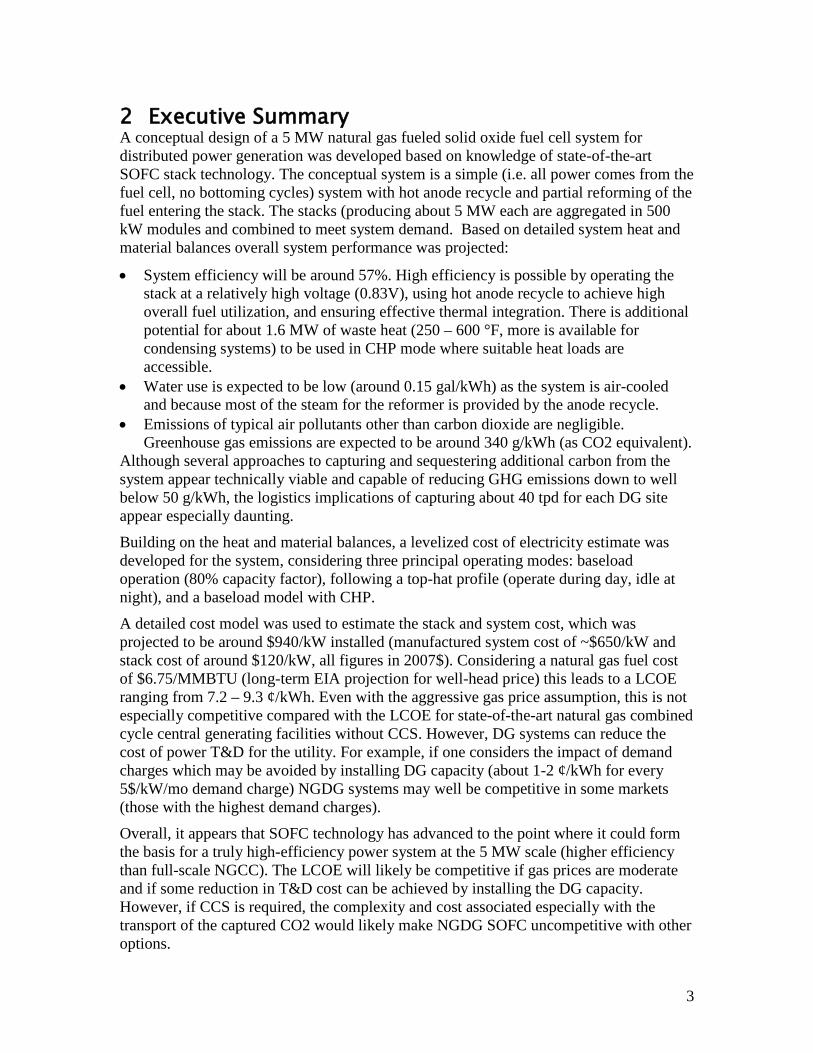


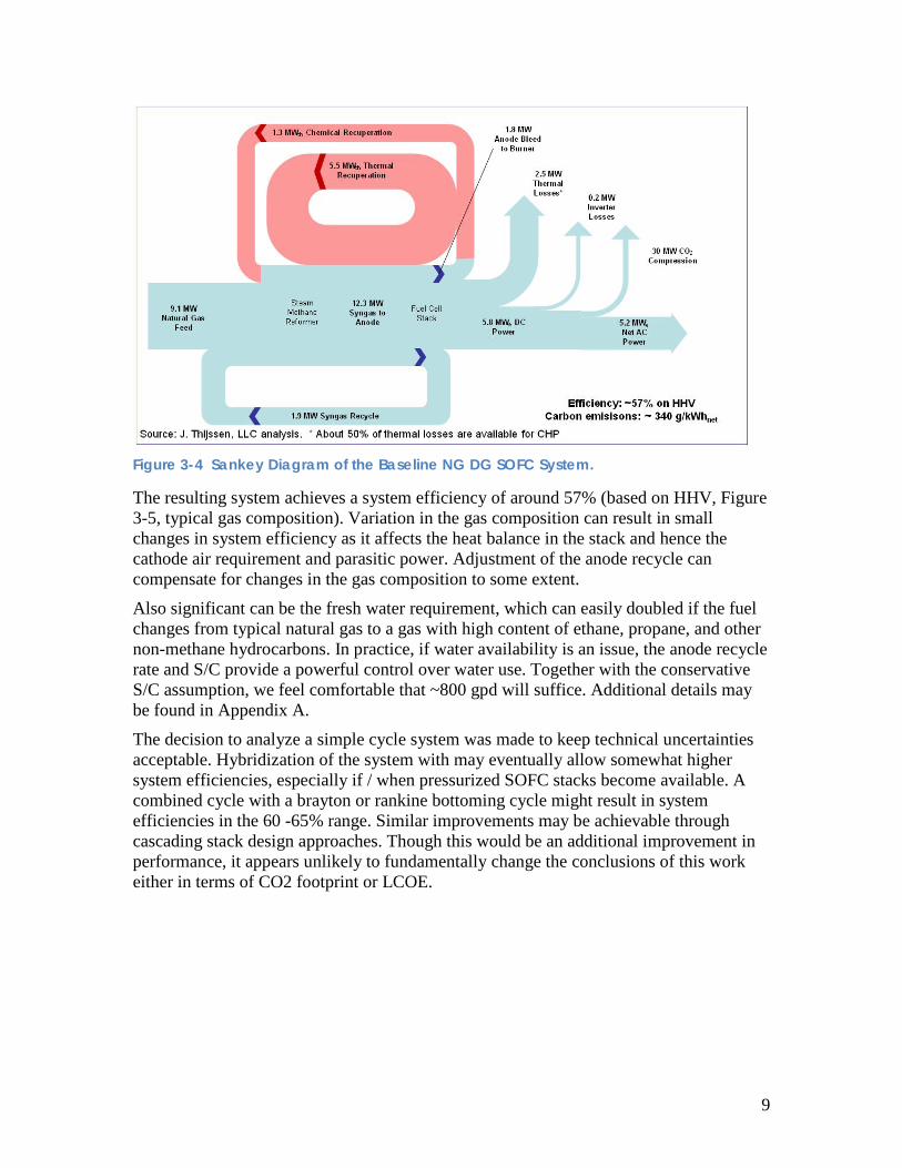


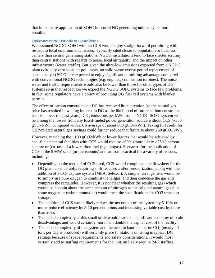


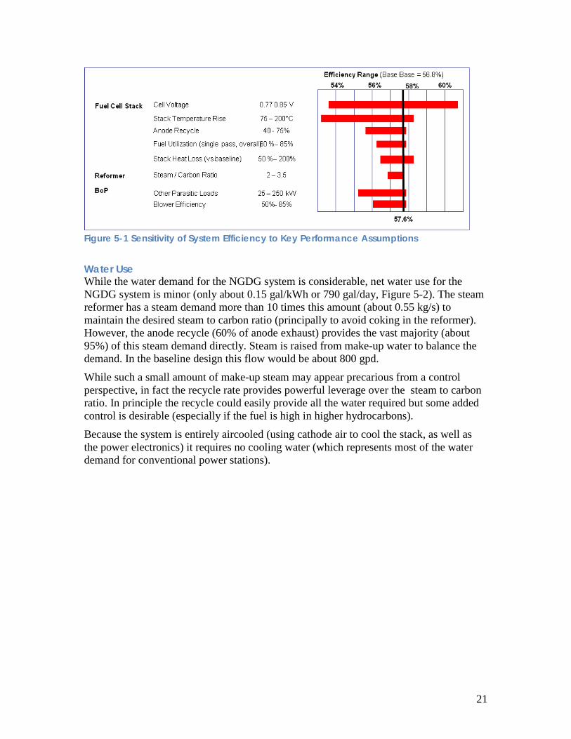


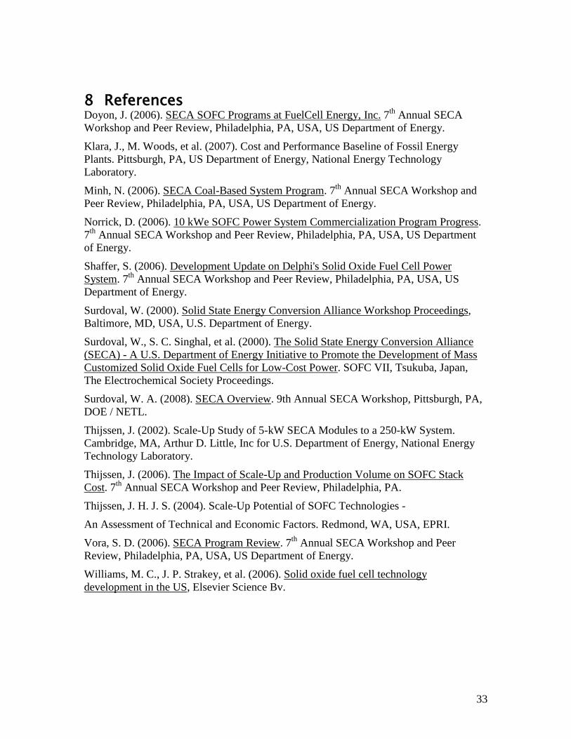


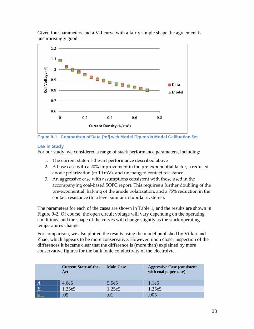


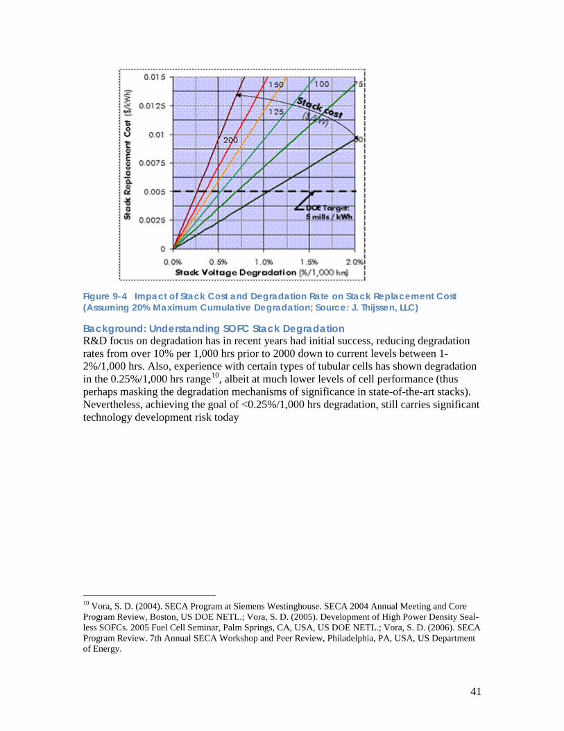

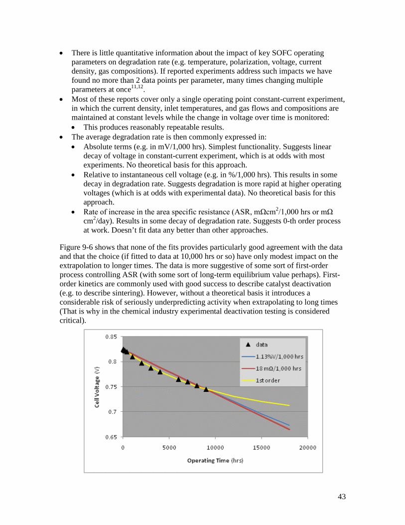
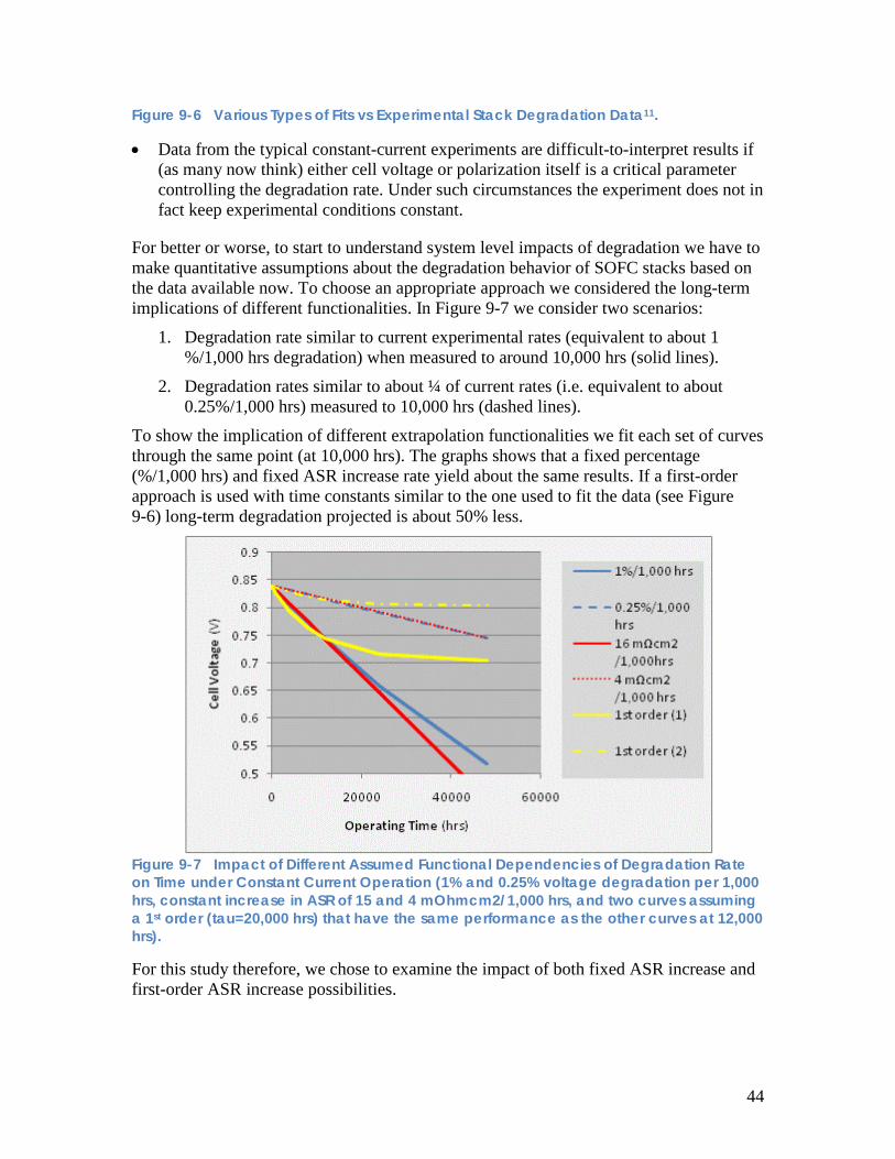


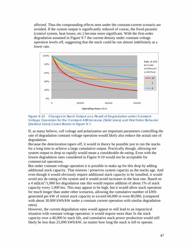


![Journal of Power Sourcesnpt.pusan.ac.kr/sites/npt/download/[46]JPS-2015-HC decomp... · 2018-03-28 · versions of gas-fueled molten carbonate fuel cells (MCFC) or solid oxide fuel](https://static.documents.pub/doc/80x56/5f064ade7e708231d417432d/journal-of-power-46jps-2015-hc-decomp-2018-03-28-versions-of-gas-fueled.jpg)


