94
Natural Resource and Environmental Economics Roger Perman Yue Ma James McGilvray Michael Common 3rd edition www.booksites.net

Natural Resource and Environmental Economics
Roger Perman Yue Ma James McGilvray Michael Common 3rd edition
Natural Resource and Environmental Economics
Roger Perman Yue Ma James McGilvray Michael Common
Natu
ral Reso
urce an
d E
nviro
nm
ental E
con
om
icsR
oger Perm
an Yue Ma Jam
es McG
ilvray Michael C
omm
on
3rd edition3rd edition
Natural Resource and Environmental Economics isamong the leading textbooks in its field. Well written andrigorous in its approach, this third edition follows in the veinof previous editions and continues to provide a compre-hensive and clear account of the application of economicanalysis to environmental issues. The new edition retains allof the topics from the second edition but has beenreorganised into four Parts: I Foundation II EnvironmentalPollution III Project Appraisal IV Natural ResourceExploitation.
This text has been written primarily for the specialistmarket of second and third year undergraduate andpostgraduate students of economics.
Roger Perman is Senior Lecturer in Economics,Strathclyde University. His major research interests andpublications are in the field of applied econometrics andenvironmental economics.
Michael Common is Professor in the Graduate School ofEnvironmental Studies at Strathclyde University. His majorresearch interests are the development of ecologicaleconomics and policies for sustainability.
Yue Ma is Associate Professor in Economics, LingnanUniversity, Hong Kong, and Adjunct Professor of LingnanCollege, Zhongshan University, China. His major researchinterests are international banking and finance, as well asenvironmental economics for developing countries.
The late James McGilvray was Professor of Economics atStrathclyde University. He made important contributions inthe fields of input-output analysis, social accounting andeconomic statistics, and to the study of the economics oftransition in Central and Eastern Europe.
www.booksites.net www.booksites.netwww.pearsoneduc.com
Features:
• New chapters on pollution control with imperfect information; cost-benefit analysis and other project appraisal tools; and stock pollution problems
• Substantial extensions to existing chapters, including a thorough account of game theory and its application to international environmental problems; fuller treatments of renewable resource and forestry economics; and greater emphasis on spatial aspects of pollution policy
• New pedagogical features including learning objectives, chapter summaries, further questions and more concise boxed cases
• New accompanying website at www.booksites.net/perman provides a rich variety of resources for both lecturers and students
• Case studies and examples are used extensively, highlighting the application of theory
• Further readings, discussion questions and problems conclude each chapter
• Detailed mathematical analysis is covered in appendices to the relevant chapters
• Writing style and technical level have been made more accessible and consistent
Cover Image ©Getty Images
www.booksites.net
Natural Resource and Environmental Economics
Third Edition
Roger PermanYue MaJames McGilvrayMichael Common

Pearson Education LimitedEdinburgh GateHarlowEssex CM20 2JE
and Associated Companies throughout the world
Visit us on the World Wide Web at:www.pearsoneduc.com
First published 1996 Longman Group LimitedSecond edition 1999 Addison Wesley Longman LimitedThird edition 2003 Pearson Education Limited
© Longman Group Limited 1996© Addison Wesley Longman Limited 1999© Pearson Education Limited 2003
The rights of Roger Perman, Yue Ma, James McGilvray andMichael Common to be identified as the authors of this workhave been asserted by them in accordance with the Copyright,Designs and Patents Act 1988.
All rights reserved. No part of this publication may be reproduced, stored in a retrieval system, or transmitted in any form or by any means, electronic, mechanical,photocopying, recording or otherwise, without either the prior written permission of thepublisher or a licence permitting restricted copying in the United Kingdom issued by theCopyright Licensing Agency Ltd, 90 Tottenham Court Road, London W1P 0LP.
ISBN 0273655590
British Library Cataloguing-in-Publication DataA catalogue record for this book is available from the British Library
Library of Congress Cataloging-in-Publication DataNatural resource and environmental economics / Roger Perman . . . [et al.].—3rd ed.
p. cm.Rev. ed. of: Natural resource and environmental economics / Roger Perman,
Yue Ma, James McGilvray. 1996.Includes bibliographical references and index.ISBN 0-273-65559-0 (pbk.)1. Environmental economics. 2. Natural resources—Management.
3. Sustainable development. I. Perman, Roger, 1949– Natural resource and environmental economics.
HC79.E5 P446 2003333.7—dc21 2002042567
10 9 8 7 6 5 4 3 2 106 05 04 03
Typeset in 9.75/12pt Times by 35Printed and bound by Ashford Colour Press Ltd., Gosport

Contents
Preface to the Third Edition xiii
Acknowledgements xv
Notation xvi
Introduction xix
Part I Foundations
Chapter 1 An introduction to natural resource and environmental economics 3
Learning objectives 3Introduction 3
1.1 Three themes 31.2 The emergence of resource and environmental economics 41.3 Fundamental issues in the economic approach to resource
and environmental issues 101.4 Reader’s guide 12
Summary 14Further reading 15
Chapter 2 The origins of the sustainability problem 16
Learning objectives 16Introduction 16
2.1 Economy–environment interdependence 172.2 The drivers of environmental impact 282.3 Poverty and inequality 412.4 Limits to growth? 442.5 The pursuit of sustainable development 48
Summary 52Further reading 52Discussion questions 54Problems 54
Chapter 3 Ethics, economics and the environment 56
Learning objectives 56Introduction 56

vi Contents
3.1 Naturalist moral philosophies 573.2 Libertarian moral philosophy 583.3 Utilitarianism 593.4 Criticisms of utilitarianism 643.5 Intertemporal distribution 67
Summary 75Further reading 75Discussion questions 76Problems 77Appendix 3.1 The Lagrange multiplier method of solving constrained optimisation problems 77Appendix 3.2 Social welfare maximisation 80
Chapter 4 Concepts of sustainability 82
Learning objectives 82Introduction 82
4.1 Concepts and constraints 834.2 Economists on sustainability 864.3 Ecologists on sustainability 924.4 The institutional conception 964.5 Sustainability and policy 97
Summary 103Further reading 103Discussion questions 104Problems 104
Chapter 5 Welfare economics and the environment 105
Learning objectives 105Introduction 105
Part I Efficiency and optimality 1055.1 Economic efficiency 1075.2 An efficient allocation of resources is not unique 1095.3 The social welfare function and optimality 1125.4 Compensation tests 113
Part II Allocation in a market economy 1165.5 Efficiency given ideal conditions 1165.6 Partial equilibrium analysis of market efficiency 1195.7 Market allocations are not necessarily equitable 122
Part III Market failure, public policy and the environment 1245.8 The existence of markets for environmental services 1245.9 Public goods 126
5.10 Externalities 1345.11 The second-best problem 1425.12 Imperfect information 1435.13 Government failure 144
Summary 145Further reading 146Discussion questions 146Problems 146Appendix 5.1 Conditions for efficiency and optimality 147

Contents vii
Appendix 5.2 Market outcomes 152Appendix 5.3 Market failure 153
Part II Environmental pollution
Chapter 6 Pollution control: targets 165
Learning objectives 165Introduction 165
6.1 Modelling pollution mechanisms 1676.2 Pollution flows, pollution stocks, and pollution damage 1696.3 The efficient level of pollution 1706.4 A static model of efficient flow pollution 1716.5 Modified efficiency targets 1746.6 Efficient levels of emissions of stock pollutants 1776.7 Pollution control where damages depend on location
of the emissions 1776.8 Ambient pollution standards 1796.9 Intertemporal analysis of stock pollution 181
6.10 Variable decay 1866.11 Convexity and non-convexity in damage and abatement
cost functions 1876.12 Estimating the costs of abating pollution 1896.13 Choosing pollution targets on grounds other than
economic efficiency 193Summary 194Further reading 195Discussion questions 196Problems 196Appendix 6.1 Matrix algebra 196Appendix 6.2 Spatially differentiated stock pollution: a numerical example 201
Chapter 7 Pollution control: instruments 202
Learning objectives 202Introduction 202
7.1 Criteria for choice of pollution control instruments 2037.2 Cost efficiency and cost-effective pollution abatement
instruments 2047.3 Instruments for achieving pollution abatement targets 2067.4 Economic incentive (quasi-market) instruments 2177.5 Pollution control where damages depend on location
of the emissions 2287.6 A comparison of the relative advantages of command
and control, emissions tax, emission abatement subsidy and marketable permit instruments 234Summary 238Further reading 239Discussion questions 240

viii Contents
Problems 241Appendix 7.1 The least-cost theorem and pollution control instruments 242
Chapter 8 Pollution policy with imperfect information 247
Learning objectives 247Introduction 247
8.1 Difficulties in identifying pollution targets in the context of limited information and uncertainty 248
8.2 Sustainability-based approaches to target setting and the precautionary principle 249
8.3 The relative merits of pollution control instruments under conditions of uncertainty 251
8.4 Transactions costs and environmental regulation 261Summary 266Further reading 267Discussion question 268Problems 268
Chapter 9 Economy-wide modelling 269
Learning objectives 269Introduction 269
9.1 Input–output analysis 2709.2 Environmental input–output analysis 2749.3 Costs and prices 2789.4 Computable general equilibrium models 281
Summary 290Further reading 290Discussion questions 290Problems 291Appendix 9.1 A general framework for environmental input–output analysis 291Appendix 9.2 The algebra of the two-sector CGE model 295
Chapter 10 International environmental problems 297
Learning objectives 297Introduction 297
10.1 International environmental cooperation 29810.2 Game theory analysis 29910.3 Factors contributing to enhancing probability of international
agreements or achieving a higher degree of cooperation 31110.4 International treaties: conclusions 31210.5 Acid rain pollution 31210.6 Stratospheric ozone depletion 31910.7 The greenhouse effect 32110.8 International trade and the environment 339
Learning outcomes 342Further reading 343Discussion questions 345
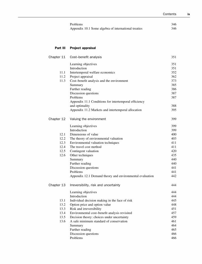
Contents ix
Problems 346Appendix 10.1 Some algebra of international treaties 346
Part III Project appraisal
Chapter 11 Cost–benefit analysis 351
Learning objectives 351Introduction 351
11.1 Intertemporal welfare economics 35211.2 Project appraisal 36211.3 Cost–benefit analysis and the environment 373
Summary 385Further reading 386Discussion questions 387Problems 387Appendix 11.1 Conditions for intertemporal efficiency and optimality 388Appendix 11.2 Markets and intertemporal allocation 395
Chapter 12 Valuing the environment 399
Learning objectives 399Introduction 399
12.1 Dimensions of value 40012.2 The theory of environmental valuation 40312.3 Environmental valuation techniques 41112.4 The travel cost method 41112.5 Contingent valuation 42012.6 Other techniques 435
Summary 440Further reading 440Discussion questions 441Problems 441Appendix 12.1 Demand theory and environmental evaluation 442
Chapter 13 Irreversibility, risk and uncertainty 444
Learning objectives 444Introduction 444
13.1 Individual decision making in the face of risk 44513.2 Option price and option value 44813.3 Risk and irreversibility 45113.4 Environmental cost–benefit analysis revisited 45713.5 Decision theory: choices under uncertainty 45913.6 A safe minimum standard of conservation 461
Summary 464Further reading 465Discussion questions 466Problems 466
x Contents
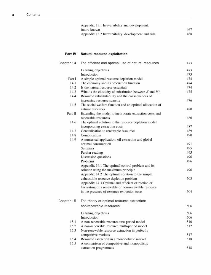
Appendix 13.1 Irreversibility and development: future known 467Appendix 13.2 Irreversibility, development and risk 468
Part IV Natural resource exploitation
Chapter 14 The efficient and optimal use of natural resources 473
Learning objectives 473Introduction 473
Part I A simple optimal resource depletion model 47414.1 The economy and its production function 47414.2 Is the natural resource essential? 47414.3 What is the elasticity of substitution between K and R? 47514.4 Resource substitutability and the consequences of
increasing resource scarcity 47614.5 The social welfare function and an optimal allocation of
natural resources 480Part II Extending the model to incorporate extraction costs and
renewable resources 48614.6 The optimal solution to the resource depletion model
incorporating extraction costs 48714.7 Generalisation to renewable resources 48914.8 Complications 49014.9 A numerical application: oil extraction and global
optimal consumption 491Summary 495Further reading 495Discussion questions 496Problems 496Appendix 14.1 The optimal control problem and its solution using the maximum principle 496Appendix 14.2 The optimal solution to the simple exhaustible resource depletion problem 503Appendix 14.3 Optimal and efficient extraction or harvesting of a renewable or non-renewable resource in the presence of resource extraction costs 504
Chapter 15 The theory of optimal resource extraction: non-renewable resources 506
Learning objectives 506Introduction 506
15.1 A non-renewable resource two-period model 51015.2 A non-renewable resource multi-period model 51215.3 Non-renewable resource extraction in perfectly
competitive markets 51715.4 Resource extraction in a monopolistic market 51815.5 A comparison of competitive and monopolistic
extraction programmes 518

Contents xi
15.6 Extensions of the multi-period model of non-renewable resource depletion 520
15.7 The introduction of taxation/subsidies 52515.8 The resource depletion model: some extensions and
further issues 52615.9 Do resource prices actually follow the Hotelling rule? 527
15.10 Natural resource scarcity 529Summary 532Further reading 533Discussion questions 533Problems 533Appendix 15.1 Solution of the multi-period resource depletion model 534Appendix 15.2 The monopolist’s profit-maximising extraction programme 535Appendix 15.3 A worked numerical example 536
Chapter 16 Stock pollution problems 537
Learning objectives 537Introduction 537
16.1 An aggregate dynamic model of pollution 53816.2 A complication: variable decay of the pollution stock 54416.3 Steady-state outcomes 54416.4 A model of waste accumulation and disposal 548
Summary 553Further reading 554Discussion question 554Problem 554
Chapter 17 Renewable resources 555
Learning objectives 555Introduction 555
17.1 Biological growth processes 55717.2 Steady-state harvests 56017.3 An open-access fishery 56117.4 The dynamics of renewable resource harvesting 56617.5 Some more reflections on open-access fisheries 56917.6 The private-property fishery 57017.7 Dynamics in the PV-maximising fishery 57817.8 Bringing things together: the open-access fishery,
static private-property fishery and PV-maximising fishery models compared 579
17.9 Socially efficient resource harvesting 58017.10 A safe minimum standard of conservation 58217.11 Resource harvesting, population collapses and the extinction
of species 58417.12 Renewable resources policy 586
Summary 592Further reading 593Discussion questions 595Problems 595

xii Contents
Appendix 17.1 The discrete-time analogue of the continuous-time fishery models examined in Chapter 17 596
Chapter 18 Forest resources 598
Learning objectives 598Introduction 598
18.1 The current state of world forest resources 59918.2 Characteristics of forest resources 60118.3 Commercial plantation forestry 60518.4 Multiple-use forestry 61218.5 Socially and privately optimal multiple-use plantation forestry 61518.6 Natural forests and deforestation 61518.7 Government and forest resources 619
Summary 619Further reading 620Discussion questions 620Problems 621Appendix 18.1 Mathematical derivations 622Appendix 18.2 The length of a forest rotation in the infinite-rotation model: some comparative statics 623
Chapter 19 Accounting for the environment 626
Learning objectives 626Introduction 627
19.1 Environmental indicators 62719.2 Environmental accounting: theory 63119.3 Environmental accounting: practice 64019.4 Sustainability indicators 65019.5 Concluding remarks 656
Further reading 658Discussion questions 659Problems 659Appendix 19.1 National income, the return on wealth, Hartwick’s rule and sustainable income 660Appendix 19.2 Adjusting national income measurement to account for the environment 663Appendix 19.3 The UNSTAT proposals 666
References 671
Index 689

PART II Environmental pollution
The use of coal was prohibited in London in 1273, and at least one person was put to deathfor this offense around 1300. Why did it take economists so long to recognize and analyze theproblem? Fisher (1981), p. 164
Introduction
In thinking about pollution policy, the economist isinterested in two major questions. How much pollu-tion should there be? And, given that some targetlevel has been chosen, what is the best method ofachieving that level? In this chapter we deal with thefirst of these questions; the second is addressed inthe next chapter.
How much pollution there should be depends onthe objective that is being sought. Many economistsregard economic optimality as the ideal objective.This requires that resources should be allocated so as to maximise social welfare. Associated with thatallocation will be the optimal level of pollution.However, the information required to establish theoptimal pollution level is likely to be unobtainable,and so that criterion is not feasible in practice.1 As a result, the weaker yardstick of economic effici-ency is often proposed as a way of setting pollutiontargets.2
CHAPTER 6 Pollution control: targets
1 In Chapter 5 we showed that identification of an optimal alloca-tion requires, among other things, knowledge of an appropriatesocial welfare function, and of production technologies and indi-vidual preferences throughout the whole economy. Moreover, evenif such an allocation could be identified, attaining it might involvesubstantial redistributions of wealth.2 If you are unclear about the difference between optimality andefficiency it might be sensible to look again at Chapter 5. It is worth
recalling that the efficiency criterion has an ethical underpinningthat not all would subscribe to, as it implicitly accepts the prevail-ing distribution of wealth. We established in Chapter 5 that efficientoutcomes are not necessarily optimal ones. Moreover, moving froman inefficient to an efficient outcome does not necessarily lead toan improvement in social well-being.
Learning objectives
At the end of this chapter, the reader should beable ton understand the concept of a pollution
targetn appreciate that many different criteria
can be used to determine pollution targets
n understand that alternative policy objectives usually imply different pollutiontargets
n understand how in principle targets may beconstructed using an economic efficiencycriterion
n understand the difference between flow andstock pollutants
n analyse efficient levels of flow pollutants andstock pollutants
n appreciate the importance of the degree ofmixing of a pollutant stock
n recognise and understand the role of spatialdifferentiation for emissions targets

166 Environmental pollution
The use of efficiency as a way of thinking abouthow much pollution there should be dates back tothe work of Pigou, and arose from his develop-ment of the concept of externalities (Pigou, 1920).Subsequently, after the theory of externalities hadbeen extended and developed, it became the mainorganising principle used by economists whenanalysing pollution problems.
In practice, much of the work done by economistswithin an externalities framework has used a partialequilibrium perspective, looking at a single activity(and its associated pollution) in isolation from therest of the system in which the activity is embedded.There is, of course, no reason why externalities can-not be viewed in a general equilibrium framework,and some of the seminal works in environmentaleconomics have done so. (See, for example, Baumoland Oates, 1988, and Cornes and Sandler, 1996.)
This raises the question of what we mean by the‘system’ in which pollution-generating activities are embedded. The development of environmentaleconomics and of ecological economics as distinctdisciplines led some writers to take a comprehensiveview of that system. This involved bringing thematerial and biological subsystems into the picture,and taking account of the constraints on economy–environment interactions.
One step in this direction came with incorporatingnatural resources into economic growth models. Thenpollution can be associated with resource extrac-tion and use, and best levels of pollution emerge in the solution to the optimal growth problem.Pollution problems are thereby given a firm materialgrounding and policies concerning pollution levelsand natural resource uses are linked. Much of thework done in this area has been abstract, at a highlevel of aggregation, and is technically difficult.Nevertheless, we feel it is of sufficient importance towarrant study, and have devoted Chapter 16 to it.3
There have been more ambitious attempts to usethe material balance principle (which was explainedin Chapter 2) as a vehicle for investigating pollu-tion problems. These try to systematically modelinteractions between the economy and the environ-ment. Production and consumption activities draw
upon materials and energy from the environment.Residuals from economic processes are returned tovarious environmental receptors (air, soils, biota andwater systems). There may be significant delays inthe timing of residual flows from and to the environ-ment. In a growing economy, a significant part of thematerials taken from the environment is assembledin long-lasting structures, such as roads, buildingsand machines. Thus flows back to the natural envir-onment may be substantially less than extractionfrom it over some interval of time. However, in thelong run the materials balance principle points toequality between outflows and inflows. If we definedthe environment broadly (to include human-madestructures as well as the natural environment) theequality would hold perfectly at all times. While the masses of flows to and from the environment are identical, the return flows are in different phys-ical forms and to different places from those of theoriginal, extracted materials. A full development ofthis approach goes beyond what we are able to coverin this book, and so we do not discuss it further(beyond pointing you to some additional reading).
Economic efficiency is one way of thinking aboutpollution targets, but it is certainly not the only way.For example, we might adopt sustainability as thepolicy objective, or as a constraint that must besatisfied in pursuing other objectives. Then pollutionlevels (or trajectories of those through time) wouldbe assessed in terms of whether they are compat-ible with sustainable development. Optimal growthmodels with natural resources, and the materials balance approach just outlined, lend themselves wellto developing pollution targets using a sustainabil-ity criterion. We will show later (in Chapters 14, 16and 19) that efficiency and sustainability criteria donot usually lead to similar recommendations aboutpollution targets.
Pollution targets may be, and in practice often are,determined on grounds other than economic effici-ency or sustainability. They may be based on whatrisk to health is deemed reasonable, or on what isacceptable to public opinion. They may be based onwhat is politically feasible. In outlining the politicaleconomy of regulation in Chapter 8, we demonstrate
3 Our reason for placing this material so late in the text is pedagogical. The treatment is technically difficult, and is best
dealt with after first developing the relevant tools in Chapters 14and 15.

Figure 6.1 describes the process steps of the oil-to-electricity fuel cycle. At each of thesesteps, some material transformation occurs, with potential for environmental, health andother damage.
The task given to the ExternE research team was, among other things, to estimate theexternal effects of power generation in Europe. A standard methodology framework – called the Impact Pathway Methodology – was devisedfor this task. The stages of the impact pathwayare shown on the left-hand side of Figure 6.2.Each form of pollutant emission associated with each fuel cycle was investigated in thisstandard framework. One example of this, forone pollutant and one kind of impact of thatpollutant, is shown on the right-hand side ofFigure 6.2; coal use results in sulphur dioxideemissions, which contribute to acidification ofair, ground and water systems.
An indication of the pervasiveness of impactsand forms of damage is shown in Table 6.1,which lists the major categories of damagesarising from the oil-to-electricity fuel cycle. Infact, ExternE identified 82 sub-categories of theitems listed in Table 6.1. It attempted to measureeach of these 82 impacts for typical oil-firedpower stations in Europe, and place a monetaryvalue on each sub-category.
ExternE (1995) compiled a detailed summaryof its estimates of the annual total damageimpacts of one example of an oil fuel cycle
Figure 6.1 Process steps of the oil-to-electricity fuel cycleSource: ExternE (1995), figure 3.1, p. 30
Box 6.1 The oil-to-electricity fuel cycle
Pollution control: targets 167
that policy is influenced, sometimes very strongly, bythe interplay of pressure groups and sectional inter-ests. Moreover, in a world in which the perceivedimportance of international or global pollution prob-lems is increasing, policy makers find themselvessetting targets within a network of obligations andpressures from various national governments andcoalitions. Pollution policy making within this inter-national milieu is the subject of Chapter 10.
In the final analysis, pollution targets are rarely, ifever, set entirely on purely economic grounds. Stand-ards setting is usually a matter of trying to attainmultiple objectives within a complex institutionalenvironment. Nevertheless, the principal objectiveof this chapter is to explain what economics has tosay about determining pollution targets.
6.1 Modelling pollution mechanisms
Before going further, it will be instructive to de-velop a framework for thinking about how pollutionemissions and stocks are linked, and how theserelate to any induced damage. An example is used to help fix ideas. Box 6.1 outlines the stages, andsome characteristics, of the oil fuel cycle. It illus-trates the material and energy flows associated withthe extraction and transportation of oil, its refiningand burning for energy generation, and the subse-quent transportation and chemical changes of theresiduals in this process.
The contents of Box 6.1 lead one to consider sev-eral important ideas that will be developed in this

168 Environmental pollution
Box 6.1 continued
of a natural gas fuel cycle (the West Burtonpower station, a 652 MW Combined Cycle GasTurbine Plant in the East Midlands of the UK).Data is shown in currency units of mecu (milli-ecu, or 0.001 ecu; at 1992 exchange rates$US 1.25 ≈ 1 ecu).
It is useful to study this material for tworeasons. First, it shows the huge breadth of typesof pollution impact, and the great attention todetail given in well-funded research studies.Second, as Table 6.2 demonstrates, estimates ofpollution damages are often dominated by valuesattributed to human mortality impacts. The datain Table 6.2 shows the sums of annual combinedimpacts of the two example power stations(expressed in units of mecu/kWh) for three verybroad impact categories, and then in terms ofpercentages of total impact. Impacts on humanmortality constitute over 78% of the identifiedand quantified impacts. It should be pointed outthat the figures shown were arrived at when theExternE analysis was incomplete; in particular,little attention had been given to greenhousewarming impacts of CO2 emissions. Nevertheless,the figures here illustrate one property that iscommon to many impact studies: human healthimpacts account for a large proportion of thetotal damage values. Given that valuation ofhuman life is by no means straightforward (as we shall indicate in Chapter 12), estimatesproduced by valuation studies can often behighly contentious.
Table 6.1 Major categories of damage arising fromthe oil-to-electricity fuel cycle
Damage category
Oil spills on marine ecosystemsPublic health:
Acute mortalityAcute morbidityOzoneChronic morbidity
Occupational healthAgricultureForestsMaterialsNoiseGlobal warming
Source: Adapted from ExternE (1995)
Table 6.2 ExternE estimates of the damage impactsof two power stations
Category Total
All Other 0.7826Death 18.4362Other human health 4.30331
Grand Total 23.5221
Category Total
All Other 3.33%Death 78.38%Other human health 18.29%
Grand Total 100.00%
Source: ExternE (1995), as compiled in the Excelworkbook ExternE.xls. Full definitions of units andvariables are given there
(the Lauffen power plant, Germany, employing a peak-load gas turbine plant operated with light fuel-oil and a base load combined cycleplant using heavy fuel-oil). Given its size – about 100 individual categories of impact areidentified – we have chosen to present thesefindings separately, in the Excel workbookExternE.xls in the Additional Materials forChapter 6. For convenience, the Excel table also contains damage estimates for one example
Figure 6.2 The impact pathways methodology and oneexampleSource: Adapted from ExternE (1995), figure 1, p. iii

Pollution control: targets 169
chapter. In particular, residual flows impose loadsupon environmental systems. The extent to whichthese waste loads generate impacts that are associ-ated with subsequent damage depends upon severalthings, including:
n the assimilative (or absorptive) capacity of thereceptor environmental media;
n the existing loads on the receptor environmentalmedia;
n the location of the environmental receptor media,and so the number of people living there and thecharacteristics of the affected ecosystems;
n tastes and preferences of affected people.
Figure 6.3 illustrates some of these ideas schemat-ically for pollution problems in general. Some pro-
Figure 6.3 Economic activity, residual flows andenvironmental damage
portion of the emission flows from economic activityis quickly absorbed and transformed by environmentalmedia into harmless forms. The assimilative capa-city of the environment will in many circumstancesbe sufficient to absorb and transform into harmlessforms some amount of wastes. However, carryingcapacities will often be insufficient to deal with allwastes in this way, and in extreme cases carryingcapacities will become zero when burdens becomeexcessive. Furthermore, physical and chemical pro-cesses take time to operate. Some greenhouse gases,for example, require decades to be fully absorbed inwater systems or chemically changed into non-warming substances (see Table 6.3).
This implies that some proportion of wastes will,in any time interval, remain unabsorbed or untrans-formed. These may cause damage at the time of their emission, and may also, by accumulating aspollutant stocks, cause additional future damage.Stocks of pollutants will usually decay into harm-less forms but the rate of decay is often very slow.The half-lives of some radioactive substances arethousands of years, and for some highly persistentpollutants, such as the heavy metals, the rate ofdecay is approximately zero.
6.2 Pollution flows, pollution stocks and pollution damage
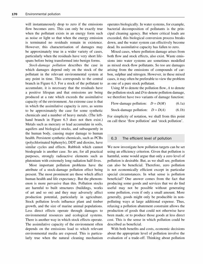
Pollution can be classified in terms of its damagemechanism. This has important implications for howpollution targets are set and for the way in whichpollution is most appropriately controlled. The distinction here concerns whether damage arisesfrom the flow of the pollutant (that is, the rate ofemissions) or from the stock (or concentration rate)of pollution in the relevant environmental medium. We define the following two classes of pollution:flow-damage pollution and stock-damage pollution(but recognise that there may also be mixed cases).
Flow-damage pollution occurs when damageresults only from the flow of residuals: that is, therate at which they are being discharged into the environmental system. This corresponds to the right-hand side branch in Figure 6.3. By definition, forpure cases of flow-damage pollution, the damage
170 Environmental pollution
will instantaneously drop to zero if the emissionsflow becomes zero. This can only be exactly truewhen the pollutant exists in an energy form such as noise or light so that when the energy emission is terminated no residuals remain in existence.However, this characterisation of damages may be approximately true in a wider variety of cases,particularly when the residuals have very short life-spans before being transformed into benign forms.
Stock-damage pollution describes the case inwhich damages depend only on the stock of the pollutant in the relevant environmental system atany point in time. This corresponds to the centralbranch in Figure 6.3. For a stock of the pollutant toaccumulate, it is necessary that the residuals have a positive lifespan and that emissions are being produced at a rate which exceeds the assimilativecapacity of the environment. An extreme case is thatin which the assimilative capacity is zero, as seemsto be approximately the case for some syntheticchemicals and a number of heavy metals. (The left-hand branch in Figure 6.3 does not then exist.)Metals such as mercury or lead accumulate in soils,aquifers and biological stocks, and subsequently inthe human body, causing major damage to humanhealth. Persistent synthetic chemicals, such as PCBs(polychlorinated biphenyls), DDT and dioxins, havesimilar cycles and effects. Rubbish which cannotbiodegrade is another case. So are, for all practicalpurposes, strongly radioactive elements such as plutonium with extremely long radiation half-lives.
Most important pollution problems have theattribute of a stock-damage pollution effect beingpresent. The most prominent are those which affecthuman health and life expectancy. But the phenom-enon is more pervasive than this. Pollution stocksare harmful to built structures (buildings, works of art and so on) and they may adversely affect production potential, particularly in agriculture.Stock pollution levels influence plant and timbergrowth, and the size of marine animal populations.Less direct effects operate through damages to environmental resources and ecological systems.There is another way in which stock effects operate.The assimilative capacity of the environment oftendepends on the emissions load to which relevantenvironmental media are exposed. This is particu-larly true when the natural cleaning mechanism
operates biologically. In water systems, for example,bacterial decomposition of pollutants is the prin-cipal cleaning agency. But where critical loads areexceeded, this biological conversion process breaksdown, and the water system can effectively becomedead. Its assimilative capacity has fallen to zero.
Mixed cases, where pollution damage arises fromboth flow and stock effects, also exist. Waste emis-sions into water systems are sometimes modelled as mixed stock-flow pollutants. So too are damagesarising from the emissions of compounds of car-bon, sulphur and nitrogen. However, in these mixedcases, it may often be preferable to view the problemas one of a pure stock pollutant.
Using M to denote the pollution flow, A to denotethe pollution stock and D to denote pollution damage,we therefore have two variants of damage function:
Flow-damage pollution: D = D(M) (6.1a)
Stock-damage pollution: D = D(A) (6.1b)
For simplicity of notation, we shall from this pointon call these ‘flow pollution’ and ‘stock pollution’.
6.3 The efficient level of pollution
We now investigate how pollution targets can be setusing an efficiency criterion. Given that pollution isharmful, some would argue that only a zero level ofpollution is desirable. But, as we shall see, pollutioncan also be beneficial. Therefore, zero pollution is not economically efficient except in particularspecial circumstances. In what sense is pollutionbeneficial? One answer comes from the fact that producing some goods and services that we do finduseful may not be possible without generating some pollution, even if only a small amount. Moregenerally, goods might only be producible in non-polluting ways at large additional expense. Thus,relaxing a pollution abatement constraint allows theproduction of goods that could not otherwise havebeen made, or to produce those goods at less directcost. This is the sense in which pollution could bedescribed as beneficial.
With both benefits and costs, economic decisionsabout the appropriate level of pollution involve theevaluation of a trade-off. Thinking about pollution

Pollution control: targets 171
as an externality arising from production or con-sumption activities makes this trade-off clear. Theefficient level of an externality is not, in general,zero as the marginal costs of reducing the externaleffect will, beyond a certain point, exceed itsmarginal benefits.
The discussion of efficient pollution targets whichfollows is divided into several parts. In the first two(Sections 6.4 and 6.5) a static modelling frameworkis used to study efficient emissions of a flow pollut-ant. This explains the key principles involved indealing with the trade-off. We next, in Section 6.6,investigate the more common – and important – caseof stock-damage pollution. Two variants of stockdamage are considered. Sections 6.7 and 6.8 dealwith those stock pollutants for which the location ofthe emission source matters as far as the pollutantstock, and so the extent of damages, is concerned.Our emphasis here will be on the spatial dimensionof pollution problems. Section 6.9 focuses on thetime dimension of pollution problems. It studieslong-lived pollutants, such as greenhouse gases,which can accumulate over time. At this stage, ourtreatment of persistent stock pollutants will be relat-ively simple. Later, in Chapter 16, a richer dynamicmodelling framework will be used to identify emis-sion targets where pollution is modelled as arisingfrom the depletion of natural resources.
6.4 A static model of efficient flow pollution
A simple static model – one in which time plays norole – can be used to identify the efficient level of aflow pollutant. In this model, emissions have bothbenefits and costs. In common with much of the pol-lution literature, the costs of emissions are calleddamages. Using a concept introduced in Chapter 5,these damages can be thought of as a negative(adverse) externality. Production entails joint prod-ucts: the intended good or service, and the associatedpollutant emissions. In an unregulated economicenvironment, the costs associated with production of the intended good or service are paid by the producer, and so are internalised. But the costs ofpollution damage are not met by the firm, are not
taken into account in its decisions, and so are extern-alities. Moreover, in many cases of interest to us, itis also the case that the externality in question is whatChapter 5 called a public bad (as opposed to a pri-vate bad), in that once it has been generated, no onecan be excluded from suffering its adverse effects.
For simplicity, we suppose that damage is inde-pendent of the time or source of the emissions andthat emissions have no effect outside the economybeing studied. We shall relax these two assumptionslater, the first in Section 6.6 and in Chapter 7, andthe second in Chapter 10.
An efficient level of emissions is one that max-imises the net benefits from pollution, where netbenefits are defined as pollution benefits minus pollution costs (or damages). The level of emissions at which net benefits are maximised is equivalent to the outcome that would prevail if the pollutionexternality were fully internalised. Therefore, theidentification of the efficient level of an adverseexternality in Figure 5.14, and the discussion sur-rounding it, is apposite in this case with an appro-priate change of context.
In the case of flow pollution, damage (D) isdependent only on the magnitude of the emissionsflow (M ), so the damage function can be specified as
D = D(M) (6.2)
Matters are a little less obvious with regard to thebenefits of pollution. Let us expand a little on theearlier remarks we made about interpreting thesebenefits. Suppose for the sake of argument that firmswere required to produce their intended final out-put without generating any pollution. This would, in general, be extremely costly (and perhaps evenimpossible in that limiting case). Now consider whatwill happen if that requirement is gradually relaxed.As the amount of allowable emissions rises, firmscan increasingly avoid the pollution abatement coststhat would otherwise be incurred. Therefore, firmsmake cost savings (and so profit increases) if theyare allowed to generate emissions in producing their goods. The larger is the amount of emissionsgenerated (for any given level of goods output), thegreater will be those cost savings.
A sharper, but equivalent, interpretation of thebenefits function runs as follows. Consider a rep-resentative firm. For any particular level of output it

172 Environmental pollution
chooses to make, there will be an unconstrainedemissions level that would arise from the cost-minimising method of production. If it were requiredto reduce emissions below that unconstrained level,and did so in the profit-maximising way, the total of production and control costs would exceed thetotal production costs in the unconstrained situation.So there are additional costs associated with emis-sions reduction. Equivalently, there are savings (orbenefits) associated with emissions increases. It isthese cost savings that we regard as the benefits ofpollution.
Symbolically, we can represent this relationshipby the function
B = B(M) (6.3)
in which B denotes the benefits from emissions.4
The social net benefits (NB) from a given level ofemissions are defined by
NB = B(M) − D(M) (6.4)
It will be convenient to work with marginal, ratherthan total, functions. Thus dB/dM (or B′(M) in analternative notation) is the marginal benefit of pollu-tion and dD/dM (or D′(M) ) is the marginal damageof pollution. Economists often assume that the totaland marginal damage and benefit functions have thegeneral forms shown in Figure 6.4. Total damage is thought to rise at an increasing rate with the sizeof the pollution flow, and so the marginal damagewill be increasing in M. In contrast, total benefitswill rise at a decreasing rate as emissions increase(because per-unit pollution abatement costs will bemore expensive at greater levels of emissions reduc-tion). Therefore, the marginal benefit of pollutionwould fall as pollution flows increase.
It is important to understand that damage orbenefit functions (or both) will not necessarily havethese general shapes. For some kinds of pollutants,in particular circumstances, the functions can havevery different properties, as our discussions inSection 6.11 will illustrate. There is also an issue
about whether the benefit function correctlydescribes the social benefits of emissions. Undersome circumstances, emissions abatement can gen-erate a so-called double dividend. If it does, themarginal benefit function as defined in this chapterwill overstate the true value of emissions benefits.For some explanation of the double dividend idea,see Box 6.3. Nevertheless, except where it is statedotherwise, our presentation will assume that the general shapes shown in Figure 6.4 are valid.
To maximise the net benefits of economic activ-ity, we require that the pollution flow, M, be chosenso that
(6.5a)
or, equivalently, that
dNB
d
d
d
d
d
( )
( )
( )
M
M
B M
M
D M
M= − = 0
4 Given our interpretation of the emissions benefit function (whichinvolves optimised emissions abatement costs at any level ofemissions below the unconstrained level), it will not be an easymatter to quantify this relationship numerically. However, there are
various ways in which emissions abatement cost functions can be estimated, as you will see in Section 6.12. And with a suitablechange of label (again, as we shall see later) abatement cost func-tions are identical to the benefit function we are referring to here.
Figure 6.4 Total and marginal damage and benefitfunctions, and the efficient level of flow pollutionemissions
Pollution control: targets 173
(6.5b)
which states that the net benefits of pollution can be maximised only where the marginal benefits ofpollution equal the marginal damage of pollution.5
This is a special case of the efficiency condition foran externality stated in Chapter 5.
The efficient level of pollution is M* (see Figure6.4 again). If pollution is less than M* the marginalbenefits of pollution are greater than the marginaldamage from pollution, so higher pollution willyield additional net benefits. Conversely, if pollutionis greater than M*, the marginal benefits of pollutionare less than the marginal damage from pollution, soless pollution will yield more net benefits.
The value of marginal damage and marginalbenefit functions at their intersection is labelled µ*in Figure 6.4. We can think of this as the equilib-rium ‘price’ of pollution. This price has a part-icular significance in terms of an efficient rate of emissions tax or subsidy, as we shall discover in the following chapter. However, as there is nomarket for pollution, µ* is a hypothetical or shadowprice rather than one which is actually revealed inmarket transactions. More specifically, a shadowprice emerges as part of the solution to an optim-isation problem (in this case the problem of choos-ing M to maximise net benefits). We could alsodescribe µ* as the shadow price of the pollutionexternality. If a market were, somehow or other, toexist for the pollutant itself (thereby internalising theexternality) so that firms had to purchase rights toemit units of the pollutant, µ* would be the efficientmarket price. Indeed, Chapter 7 will demonstratethat µ* is the equilibrium price of tradable permits ifan amount M* of such permits were to be issued.
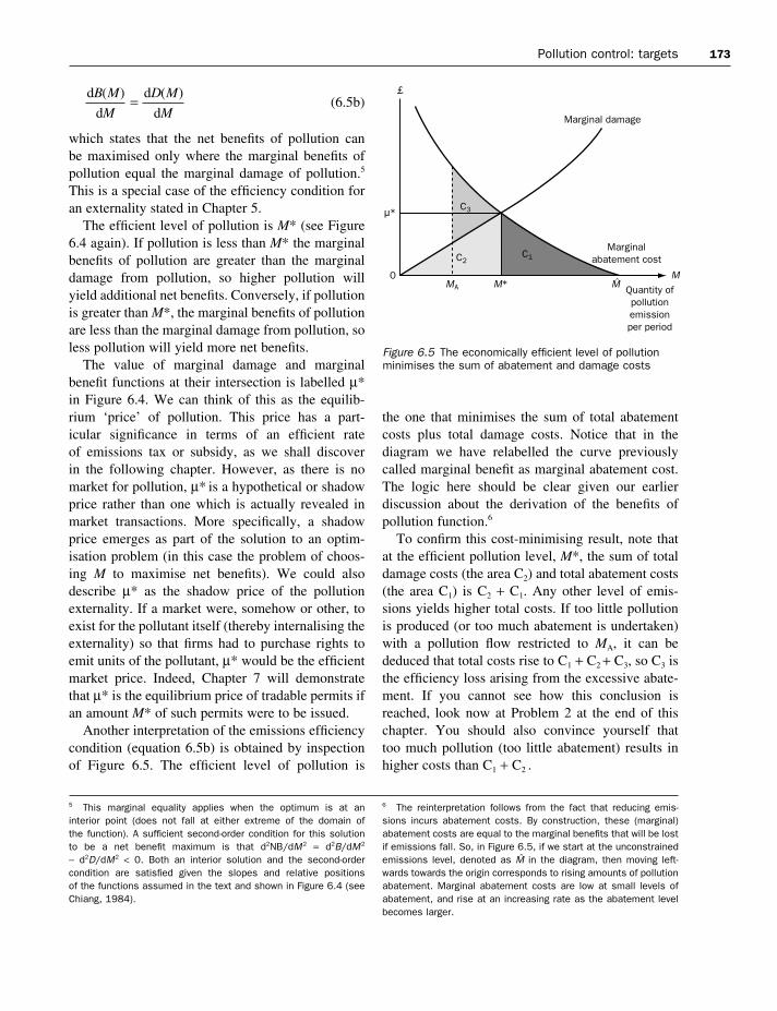
Another interpretation of the emissions efficiencycondition (equation 6.5b) is obtained by inspectionof Figure 6.5. The efficient level of pollution is
d
d
d
d
B M
M
D M
M
( )
( )=
the one that minimises the sum of total abatementcosts plus total damage costs. Notice that in the diagram we have relabelled the curve previouslycalled marginal benefit as marginal abatement cost.The logic here should be clear given our earlier discussion about the derivation of the benefits ofpollution function.6
To confirm this cost-minimising result, note thatat the efficient pollution level, M*, the sum of totaldamage costs (the area C2) and total abatement costs(the area C1) is C2 + C1. Any other level of emis-sions yields higher total costs. If too little pollutionis produced (or too much abatement is undertaken)with a pollution flow restricted to MA, it can bededuced that total costs rise to C1 + C2 + C3, so C3 isthe efficiency loss arising from the excessive abate-ment. If you cannot see how this conclusion isreached, look now at Problem 2 at the end of thischapter. You should also convince yourself that too much pollution (too little abatement) results inhigher costs than C1 + C2 .
5 This marginal equality applies when the optimum is at an interior point (does not fall at either extreme of the domain of the function). A sufficient second-order condition for this solution to be a net benefit maximum is that d2NB/dM2 = d2B/dM2
− d2D/dM2 < 0. Both an interior solution and the second-order condition are satisfied given the slopes and relative positions of the functions assumed in the text and shown in Figure 6.4 (seeChiang, 1984).
6 The reinterpretation follows from the fact that reducing emis-sions incurs abatement costs. By construction, these (marginal)abatement costs are equal to the marginal benefits that will be lostif emissions fall. So, in Figure 6.5, if we start at the unconstrainedemissions level, denoted as K in the diagram, then moving left-wards towards the origin corresponds to rising amounts of pollutionabatement. Marginal abatement costs are low at small levels ofabatement, and rise at an increasing rate as the abatement levelbecomes larger.
Figure 6.5 The economically efficient level of pollutionminimises the sum of abatement and damage costs

174 Environmental pollution
6.5 Modified efficiency targets
Our notion of efficiency to this point has been acomprehensive one; it involves maximising the difference between all the benefits of pollution andall the costs of pollution. But, sometimes, one par-ticular kind of pollution cost (or damage) is regardedas being of such importance that pollution costsshould be defined in terms of that cost alone. In thiscase we can imagine a revised or modified efficiencycriterion in which the goal is to maximise the differ-ence between all the benefits of pollution and thisparticular kind of pollution damage.
Policy makers sometimes appear to treat risks tohuman health in this way. So let us assume policymakers operate by making risks to human health theonly damage that counts (in setting targets). Howwould this affect pollution targets? The answerdepends on the relationship between emissions and
It can also be deduced from Figures 6.4 and 6.5that the efficient level of pollution will not, in gen-eral, be zero. (By implication, the efficient level ofpollution abatement will not, in general, correspondto complete elimination of pollution.) Problem 1examines this matter.
We round off this section with a simple numericalexample, given in Box 6.2. Functional forms used inthe example are consistent with the general forms of marginal benefit and marginal damage functionsshown in Figure 6.4. We solve for the values of M*,B*, D* and µ* for one set of parameter values. Alsoprovided, in the Additional Materials that are linked to this text, is an Excel spreadsheet (Targets examples.xls) that reproduces these calculations.The Excel workbook is set up so that comparativestatics analysis can be done easily by the reader.That is, the effects on M*, B*, D* and µ* of changesin parameter values from those used in Box 6.2 canbe obtained.
Box 6.2 Efficient solution for a flow pollutant: a numerical example
Suppose that the total damage and total benefitsfunctions have the following particular forms:
D = M2 for M ≥ 0
What is M*?
If M is less than or equal to 240, then we have B = 96M − 0.2M2 and so dB/dM = 96 − 0.4M. For any positive value of M we also have D = M 2 which implies that dD/dM = 2M, Now setting dB/dM = dD/dM we obtain 96 − 0.4M = 2M, implying that M* = 40.
Substituting M* = 40 into the benefit anddamage functions gives us the result that B* = 3520 and D* = 1600, and so maximised total net benefits (NB*) are 1920. Note also thatat M* marginal benefit and marginal damage are equalised at 80 and so the shadow price µ* – the value of value of marginal pollutiondamage at the efficient outcome – is 80.
You should now verify that M* = 40 is a global optimum. This can be done by sketchingthe respective marginal functions and showing
B M M MM
.
= − ≤ ≤>
96 0 2 0 24011 520 240
2 for for
that net benefits are necessarily lower than 1920for any (positive) level of M other than 40.
Additional materials
It can be useful to write a spreadsheet to dothe kind of calculations we have just gonethrough. Moreover, if the spreadsheet isconstructed appropriately, it can also serveas a template by means of which similarcalculations can be quickly implemented as required. Alternatively, we could usesuch a spreadsheet to carry out comparativestatics; that is, to see how the solutionchanges as parameter values are altered.
We have provided an Excel workbookTargets examples.xls that can be used inthese ways in the Additional Materialsavailable on the textbook’s web pages. Thatspreadsheet also shows how one of Excel’stools – ‘Solver’ – can be used to obtain theefficient level of M directly, by finding thelevel of M which maximises the net benefitfunction NB = B − D = (96M − 0.2M2 ) − (M2).

Pollution control: targets 175
Figure 6.6 Setting targets according to an absolutehealth criterion
Figure 6.7 A ‘modified efficiency-based’ health standard
health risks. One possible relationship is that illus-trated by the -shaped relationship in Figure 6.6.Total (and marginal) health risks are zero below thethreshold, but at the threshold itself risks to humanhealth become intolerably large. It is easy to see thatthe value of marginal benefits is irrelevant here. Amodified efficiency criterion would, in effect, lead to the emissions target being set by the damagethreshold alone. Target setting is simple in this case because of the strong discontinuity we haveassumed about human health risks. It is easy to see
why an absolute maximum emission standard isappropriate.
But now suppose that marginal health damage is a rising and continuous function of emissions, asin Figure 6.7. A trade-off now exists in which lowerhealth risks can be obtained at the cost of some lossof pollution benefits (or, if you prefer lower healthrisks involve higher emission abatement costs). It isnow clear that with such a trade-off, both benefitsand costs matter. A ‘modified efficiency target’ wouldcorrespond to emissions level MH*.
It is sometimes possible to achieveenvironmental objectives at no cost or, betterstill, at ‘negative’ cost. Not surprisingly, ways ofdoing things that have such effects are known as‘no regrets’ policies. There are several reasonswhy these may arise:
n double dividends;n elimination of technical and economic
inefficiencies in the energy-using or energy-producing sectors;
n induced technical change;n achievement of additional ancillary benefits,
such as improved health or visual amenity.
We will explain these ideas in the context of one potential example: reducing the emissions of carbon dioxide to reduce global climatechange. First, the ‘double dividend’ hypothesis is explained.
The double dividend hypothesis
The double dividend idea arises from thepossibility that the revenues from an emissionstax (or a system of permits sold by auction) couldbe earmarked to reduce marginal rates of othertaxes in the economy. If those other taxes havedistortionary (i.e. inefficiency-generating) effects,then reducing their rate will create efficiencygains. Thus an environmental tax with revenuesring-fenced for reducing distortionary taxes has a double benefit (dividend); the environment isimproved and efficiency gains accrue to theeconomy as whole.
There are other reasons why ‘no regret’ optionsmay be available. The existence of marketimperfections can cause firms to be producingaway from the frontier of what is technicallyand/or economically possible. Firms may beunaware of new techniques, or poorly informed
Box 6.3 No regrets and a double dividend from environmental control?
176 Environmental pollution
Box 6.4 Measures of stocks and flows for a variety of pollutants
7 A metric tonne is equal to 1000 kilograms (kg). Commonly used units for large masses are (i) a gigatonne (Gt) whichis 109 tonnes, (ii) a megatonne (Mt) which is 106 tonnes, and (iii) a petragram (Pg) which is equal to 1 Gt. Finally, 1 GtC = 3.7 Gt carbon dioxide.
Pollutant emissions are measured (like all flows) in rates of output per period of time. For example, it is estimated that worldwideanthropogenic emissions of carbon dioxide, the most important greenhouse gas, were 6.9 gigatonnes of carbon equivalent per year (6.9 GtC/yr) as of 1990.7 These flows accumulatethrough time as pollutant stocks, measured eitherin quantities in existence at some point in time,or in terms of some measure of concentration in an environmental medium of interest to us.Carbon dioxide atmospheric concentrations have
risen from about 280 ppmv (parts per million byvolume) in 1750 (the start of the industrial era) to 367 ppmv in 1999 (an increase of 31%). Thecurrent rate of change of the CO2 concentrationrate is estimated to be 1.5 ppmv per year (a growth rate of 0.4% per year). IPCC scenariossuggest that by 2100, concentrations will be inthe range 549 to 970 ppm (90 to 250% above pre-industrial levels).
Sources: Technical Summary of the Working Group 1Report (IPCC(1), 2001), particularly Figure 8, p. 36
Box 6.3 continued
about waste recycling mechanisms. Companiesmay have old, technologically obsolete capital,but are unable because of credit marketimperfections to update even when that would generate positive net present value. Anenvironmental programme that requires firms to use new, less polluting techniques, or whichprovides incentives to do so, can generate adifferent kind of double benefit. Pollution isreduced and productive efficiency gains aremade.
One special case of this is dynamic efficiencygains, arising through induced technical change.It has long been recognised (see, for example,Porter, 1991) that some forms of regulatoryconstraint may induce firms to be moreinnovative. If a pollution control mechanism canbe devised that accelerates the rate of technicalchange, then the mechanism may more than payfor itself over the long run. One area where thismay be very important is in policy towards thegreenhouse effect. Grubb (2000) arguespersuasively that the provisions of the KyotoProtocol will have beneficial induced effects ontechnical change. He writes:
general economic processes of internationalinvestment and the dissemination of technologiesand ideas – accelerated by the provisions ontechnology transfer and other processes under theConvention and the Protocol – could contribute to global dissemination of cleaner technologies
and practices. In doing so, they will also yieldmultiplicative returns upon industrialisedcountry actions.
Grubb (2000), p. 124
More generally, there is a large set of possibleancillary benefits to environmental reforms.Perhaps the most important type is healthbenefits. Reductions of greenhouse gases tend togo hand in hand with reductions in emissions of secondary pollutants (such as particulates,sulphur dioxide, nitrogen dioxide and carbonmonoxide), which can have important healthimpacts.
Some writers distinguish between a ‘weakform’ and a ‘strong form’ of the double dividendhypothesis. For a revenue-neutral environmentalreform, the weak form refers to the case wheretotal real resource costs are lower for a schemewhere revenues are used to reduce marginal ratesof distortionary taxes than where the revenuesare used to finance lump-sum payments tohouseholds or firms. There is almost universalagreement that this hypothesis is valid. Thestrong form asserts that the real resource costs of a revenue-neutral environmental tax reformare zero or negative. Not surprisingly, thishypothesis is far more contentious.
For a more thorough examination of the doubledividend hypothesis, and some empirical results,see the Word file Double Dividend in AdditionalMaterials, Chapter 6.

Pollution control: targets 177
6.6 Efficient levels of emission of stock pollutants
The analysis of pollution in Section 6.4 dealt withthe case of flow pollution, in which pollution dam-age depends directly on the level of emissions. Indoing so, there were two reasons why it was unneces-sary to distinguish between flows and stocks of thepollutant. First, both benefits and damages dependedon emissions alone, so as far as the objective of netbenefit maximisation was concerned, stocks – evenif they existed – were irrelevant. But we also arguedthat, strictly speaking, stocks do not exist for pureflow pollutants (such as noise or light).
How do we need to change the analysis in the caseof stock pollutants where damage depends on thestock level of the pollutant? It turns out to be thecase – as we shall see below – that the flow pollutionmodel also provides correct answers in the special(but highly unlikely) case where the pollutant stockin question degrades into a harmless form more-or-less instantaneously. In that case, the stock dimensionis distinguishable from the flow only by some con-stant of proportionality, and so we can work just asbefore entirely in flow units. But in all other cases ofstock pollutants, the flow pollution model is invalid.
The majority of important pollution problems areassociated with stock pollutants. Pollution stocksderive from the accumulation of emissions that havea finite life (or residence time). The distinctionbetween flows and stocks now becomes crucial fortwo reasons. First, without it understanding of thescience lying behind the pollution problem is impos-
sible. Second, the distinction is important for policypurposes. While the damage is associated with thepollution stock, that stock is outside the direct controlof policy makers. Environmental protection agenciesmay, however, be able to control the rate of emissionflows. Even where they cannot control such flowsdirectly, the regulator may find it more convenient to target emissions rather than stocks. Given thatwhat we seek to achieve depends on stocks but whatis controlled or regulated are typically flows, it isnecessary to understand the linkage between the two.
As we shall now demonstrate, the analysis ofstock pollution necessitates taking account of spaceand time. For clarity of presentation it will be con-venient to deal with these two dimensions separately.To do so, we draw a distinction between pollutantswith a relatively short residence time (of the order ofa day or so) and those with considerably longer life-times (years rather than days, let us say). Table 6.3provides some idea of the active life expectancy of arange of pollutants under normal conditions.
6.7 Pollution control where damages depend on location of the emissions
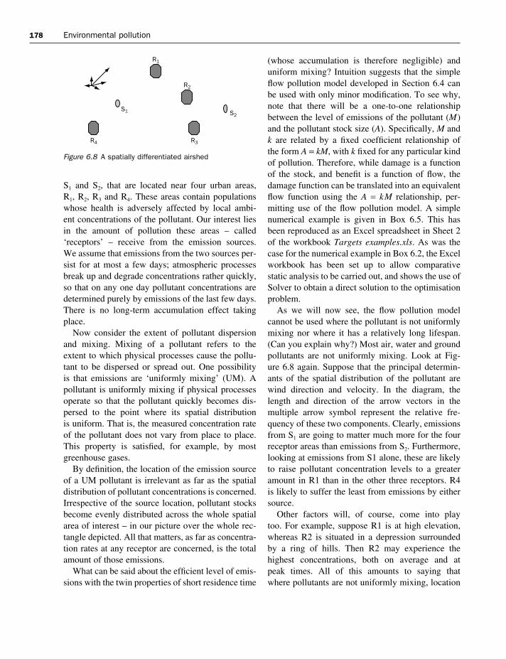
In this section and the next we deal with stock pol-lutants which have relatively short residence timesin the environmental media into which they aredumped. To help fix ideas, consider the graphic inFigure 6.8 which represents two polluting ‘sources’,
Table 6.3 Expected lifetimes for several pollutants
Pre-industrial Concentration Rate of Atmosphericconcentration in 1998 concentration change lifetime
CO2 (carbon dioxide) about 280 ppm 365 ppm 1.5 ppm/yr 5 to 200 yr1
CH4 (methane) about 700 ppb 1745 ppb 7.0 ppb/yr 12 yrN2O (nitrous oxide) about 270 ppb 314 ppb 0.8 ppb/yr 114 yrCFC-11 (chlorofluorocarbon-11) zero 268 ppt −1.4 ppt/yr 45 yrHFC-23 (hydrofluorocarbon-23) zero 14 ppt 0.55 ppt/yr 260 yrCF4 (perfluoromethane) 40 ppt 80 ppt 1 ppt/yr >50 000 yrSulphur Spatially variable Spatially variable Spatially variable 0.01 to 7 daysNOX Spatially variable Spatially variable Spatially variable 2 to 8 days
Note:1. No single lifetime can be defined for CO2 because of the different rates of uptake by different removal processesSources: Technical Summary of the IPCC Working Group 1 Report, IPCC(1) (2001), Table 1, p. 38
178 Environmental pollution
S1 and S2, that are located near four urban areas, R1, R2, R3 and R4. These areas contain populationswhose health is adversely affected by local ambi-ent concentrations of the pollutant. Our interest liesin the amount of pollution these areas – called‘receptors’ – receive from the emission sources. We assume that emissions from the two sources per-sist for at most a few days; atmospheric processesbreak up and degrade concentrations rather quickly,so that on any one day pollutant concentrations aredetermined purely by emissions of the last few days.There is no long-term accumulation effect takingplace.
Now consider the extent of pollutant dispersionand mixing. Mixing of a pollutant refers to theextent to which physical processes cause the pollu-tant to be dispersed or spread out. One possibility is that emissions are ‘uniformly mixing’ (UM). Apollutant is uniformly mixing if physical processesoperate so that the pollutant quickly becomes dis-persed to the point where its spatial distribution is uniform. That is, the measured concentration rateof the pollutant does not vary from place to place.This property is satisfied, for example, by mostgreenhouse gases.
By definition, the location of the emission sourceof a UM pollutant is irrelevant as far as the spatialdistribution of pollutant concentrations is concerned.Irrespective of the source location, pollutant stocksbecome evenly distributed across the whole spatialarea of interest – in our picture over the whole rec-tangle depicted. All that matters, as far as concentra-tion rates at any receptor are concerned, is the totalamount of those emissions.
What can be said about the efficient level of emis-sions with the twin properties of short residence time
(whose accumulation is therefore negligible) anduniform mixing? Intuition suggests that the simpleflow pollution model developed in Section 6.4 canbe used with only minor modification. To see why,note that there will be a one-to-one relationshipbetween the level of emissions of the pollutant (M)and the pollutant stock size (A). Specifically, M andk are related by a fixed coefficient relationship of the form A = kM, with k fixed for any particular kindof pollution. Therefore, while damage is a functionof the stock, and benefit is a function of flow, thedamage function can be translated into an equivalentflow function using the A = kM relationship, per-mitting use of the flow pollution model. A simplenumerical example is given in Box 6.5. This hasbeen reproduced as an Excel spreadsheet in Sheet 2of the workbook Targets examples.xls. As was thecase for the numerical example in Box 6.2, the Excelworkbook has been set up to allow comparativestatic analysis to be carried out, and shows the use ofSolver to obtain a direct solution to the optimisationproblem.
As we will now see, the flow pollution model cannot be used where the pollutant is not uniformlymixing nor where it has a relatively long lifespan.(Can you explain why?) Most air, water and groundpollutants are not uniformly mixing. Look at Fig-ure 6.8 again. Suppose that the principal determin-ants of the spatial distribution of the pollutant arewind direction and velocity. In the diagram, thelength and direction of the arrow vectors in the multiple arrow symbol represent the relative fre-quency of these two components. Clearly, emissionsfrom S1 are going to matter much more for the fourreceptor areas than emissions from S2. Furthermore,looking at emissions from S1 alone, these are likelyto raise pollutant concentration levels to a greateramount in R1 than in the other three receptors. R4 is likely to suffer the least from emissions by eithersource.
Other factors will, of course, come into play too. For example, suppose R1 is at high elevation,whereas R2 is situated in a depression surrounded by a ring of hills. Then R2 may experience the highest concentrations, both on average and at peak times. All of this amounts to saying that where pollutants are not uniformly mixing, location
Figure 6.8 A spatially differentiated airshed

Pollution control: targets 179
matters. There will not be a single relationshipbetween emissions and concentration over all space.A given total value of M will in general lead to dif-ferentiated values of A across receptors. Moreover,if M remained constant but its source distributionchanged then the spatial configuration of A wouldalso change.
Non-uniform mixing is of great importance asmany types of pollution fall into this category.Examples include ozone accumulation in the loweratmosphere, oxides of nitrogen and sulphur in urbanairsheds, particulate pollutants from diesel enginesand trace metal emissions. Many water and groundpollutants also do not uniformly mix. An environ-mental protection agency (EPA) may attempt tohandle these spatial issues by controlling ex antethe location of pollution creators and victims. This approach, implemented primarily by zoningand other forms of planning control, forms a sub-stantial part of the longer-term way of dealing with spatial aspects of pollution. However, in the nextsection we focus on the situation in which the location of polluters and people is already deter-mined, and moving either is not a feasible option.Our interest must then lie in how targets for emis-sions from the various sources can be calculated
(and, in the next chapter, on what instruments can be used).
6.8 Ambient pollution standards
It will be convenient to use a little elementary matrixalgebra for the exposition of the arguments that fol-low. For the reader unfamiliar with matrix algebra,or who needs a quick refresher, a brief appendix isprovided at the end of this chapter (Appendix 6.1)explaining the notation used in matrix algebra andstating some simple results. It would be sensible toread that now.
Some additional notation is now required. Usingearlier terminology, we regard the environment as aseries of spatially distinct pollution ‘reception’ areas(or receptors). Suppose that there are J distinctreceptors, each being indexed by the subscript j (soj = 1, 2, . . . , J) and N distinct pollution sources,each being indexed by the subscript i (so i = 1, 2,. . . , N). Various physical and chemical processesdetermine the impact on pollutant concentration inany particular receptor from any particular source.For simplicity, we assume that the relationships
Box 6.5 Efficient solution for a uniformly mixed and short-lived stock pollutant: a numerical example
As in Box 6.2 we suppose that total benefitsfunction is given by:
Our total damage, however, now needs to bespecified appropriately for a stock pollutant andis taken to be:
D = 0.2A2 for A ≥ 0
and in steady state we assume that A = 2M
What are M* and A*?
We first consider the case in which there is aninterior solution with M positive but less than240. The relevant first derivatives are:
dB/dM = 96 − 0.4M
B M M MM
.
= − ≤ ≤>
96 0 2 0 24011 520 240
2 for for
dD/dM = 1.6M
(as D = 0.2A2 implies D = 0.2 × (2M)2 = 0.8M2
which implies dD/dM = 1.6M ).Now setting dB/dM = dD/dM we obtain:
96 − 0.4M = 1.6M → M* = 48 and so A* = 96
Additional materials
As we remarked at the end of Box 6.2, aspreadsheet can be used for obtainingsolutions to problems of this kind, or forcarrying out comparative statics. Sheet 2 ofthe Excel workbook Targets examples.xlssets up a template for simple stock pollutionmodels of this form. The interested readermay find it helpful to explore that sheet.

180 Environmental pollution
are linear. In that case, a set of constant ‘transfercoefficients’ can be defined. The transfer coefficientdji describes the impact on pollutant concentration atreceptor j attributable to source i.8 The total level, or concentration rate, of pollution at location j, Aj,will be the sum of the contributions to pollution atthat location from all N emission sources. This canbe written as
(6.6)
where Mi denotes the total emissions from source i.A numerical example will help. In the case shown
in Figure 6.8, we have N = 2 sources and J = 4 recep-tors. Then we have four equations corresponding toequation 6.6. These are
A1 = d11M1 + d12M2 (6.7a)
A2 = d21M1 + d22M2 (6.7b)
A3 = d31M1 + d32M2 (6.7c)
A4 = d41M1 + d42M2 (6.7d)
We can collect all eight dji coefficients into a J × Nmatrix, D. Denoting the vector of emissions from the two sources as M and the vector of ambient pollution levels in the four receptors as A we have
A = DM (6.8)
or
(6.9)
Knowledge of the M vector and the D matrix allowsus to calculate ambient pollution levels at eachreceptor. If, for example, D and M are
D M
. .
. .
. .
. .
=
=
0 7 0 10 9 0 20 3 0 20 1 0 0
1020
and
AAAA
d dd dd dd d
MM
1
2
3
4
11 12
21 22
31 32
41 42
1
2
=
A d Mj ji ii
N
==∑
1
then A1 = 9, A2 = 13, A3 = 7 and A4 = 1. The Excelworkbook Matrix.xls and Word file Matrix.doc inAdditional Materials, Chapter 6, illustrate how this– and other similar – matrix calculations can be doneusing a spreadsheet program.
Armed with this terminology, we now answer thefollowing question in a general way: what is thesocially efficient level of emissions from eachsource? As in all previous cases in this chapter, itwill be the set of emission levels that maximises netbenefits. To see how this works here, note that thereare N emission sources, and so our solution will con-sist of N values of Mi, one for each source. Benefitsconsist of the sum over all N sources of each firm’spollution benefits. So we have
Damages consist of the sum over all J receptor areasof the damage incurred in that area. That is,
Hence the net benefits function to be maximised (byappropriate choice of Mi, i = 1, . . . , N) is
(6.10)
By substitution of equation 6.6 into 6.10, the lattercan be written as
(6.11)
A necessary condition for a maximum is that
for i = 1, . . . , N
(6.12)
= ′ − ′ = ==
∑ ( ) ( ) , . . . , B M D A d i Ni i j j jij
J
0 11
for
∂∂NB d
dMB M D A
A
Mii i j j
j
ij
J
( ) ( ) = ′ − ′ ==
∑ 01
NB ( ) = −
= = =∑ ∑ ∑B M D d Mi ii
N
jj
J
ji ii
N
1 1 1
NB ( ) ( )= −= =∑ ∑B M D Ai ii
N
j jj
J
1 1
D D Aj jj
J
( )==
∑1
B B Mi ii
N
( )==∑
1
However, if we measure average values of these coefficients oversome period of time, they can be regarded as constant coefficientsfor the purposes of our analysis.
8 The linearity assumption is a very good approximation for mostpollutants of interest. (Low-level ozone accumulation is onesignificant exception.) Each coefficient dji will, in practice, vary overtime, depending on such things as climate and wind conditions.

Pollution control: targets 181
which, after rearranging, yields the set of N marginalconditions
Where
(6.13)
The intuition behind this result is straightforward.The emissions target (or standard) for each firmshould be set so that the private marginal benefit ofits emissions (the left-hand side of the equation) isequal to the marginal damage of its emissions (theright-hand side of the equation). Note that becausethe ith firm’s emissions are transferred to some or allof the receptors, the marginal damage attributable tothe ith firm is obtained by summing its contributionto damage over each of the J receptors.
An interesting property of the solution to equationset 6.13 is that not only will the efficient emissionlevel differ from firm to firm, but also the efficientambient pollution level will differ among receptors.It is easy to see why efficient emission levels shouldvary. Firms located at different sources have dif-ferent pollution impacts: other things being equal,those sources with the highest pollution impactshould emit the least. But what lies behind the resultthat efficient levels of pollution will vary from placeto place? Receptors at different spatial locations will experience different pollution levels: otherthings being equal, those receptors which would (in an unconstrained world) experience the highestpollution-stock level should have the highest effi-cient ambient pollution level. Of course, these twoconsiderations have to be met jointly; NB = B − Dis being maximised, and so we are searching for thebest trade-off between the benefits reduction anddamages reduction. Appendix 6.2 provides a workednumerical example of efficient emissions that illus-trates this point.
In practice, environmental regulators might deemthat it is unethical for A to vary from place to place.So, they might impose an additional constraint onthe problem to reflect this ethical position. One formof constraint is that the pollution level in no areashould exceed some maximum level A* (that is Aj* ≤ A* for all j). Another, stricter, version would be
′ =D AD
Aj j
j
j
( ) ∂∂
′ = ′ ==
∑B M D A d i Ni i j j jij
J
( ) ( ) , . . . , for 11
the requirement that A should be the same over allareas (that is Aj* = A* for all j). In the latter case, thenet benefit function to be maximised is
(6.14)
By imposing additional constraints, maximised netbenefit is lower in equation 6.14 than in equation6.10. An efficiency loss has been made in return forachieving an equity goal.
6.9 Intertemporal analysis of stock pollution
We now consider the case of stock pollutants thathave a relatively long active (i.e. damaging) lifespanbut which are uniformly mixing. Doing so has twoimplications. First, the uniformly mixing assump-tion implies that pollutant concentrations will notdiffer from place to place, and so the spatial dimen-sion of emissions control is no longer of direct relev-ance. Second, persistence of pollution stocks overtime means that the temporal dimension is of centralimportance. As we shall see, an efficient pollutioncontrol programme will need to take account of thetrajectory of emissions over time, rather than just ata single point in time.
The model we use to examine pollution targets is the simplest possible one that can deal with theintertemporal choices involved. Damage at time tis determined by the contemporaneous stock size or concentration rate of the pollutant in a relevantenvironmental medium. Gross benefits depend on theflow of emissions. Hence our damage and (gross)benefit functions have the general forms
Dt = D(At ) (6.15)
Bt = B(Mt) (6.16)
The variables A and M in equations 6.15 and 6.16 are, of course, not independent of one another.With relatively long-lived pollutants, emissions addto existing stocks and those stocks accumulate overtime. However, except in the special case where pol-lutants are infinitely long-lived, part of the existingstock will decay or degrade into a harmless form
L B M D Ai ii
N
jj
J
( ) ( *)= −= =∑ ∑
1 1
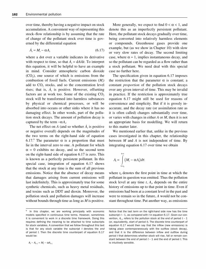
182 Environmental pollution
over time, thereby having a negative impact on stockaccumulation. A convenient way of representing thisstock–flow relationship is by assuming that the rateof change of the pollutant stock over time is gov-erned by the differential equation
At = Mt − αAt (6.17)
where a dot over a variable indicates its derivativewith respect to time, so that At = dA/dt. To interpretthis equation, it will be helpful to have an examplein mind. Consider atmospheric carbon dioxide(CO2), one source of which is emissions from thecombustion of fossil fuels. Current emissions (Mt)add to CO2 stocks, and so the concentration levelrises; that is, At is positive. However, offsetting factors are at work too. Some of the existing CO2
stock will be transformed into harmless substancesby physical or chemical processes, or will beabsorbed into oceans or other sinks where it has nodamaging effect. In other words, part of the pollu-tion stock decays. The amount of pollution decay iscaptured by the term −αAt.
The net effect on A (and so whether At is positiveor negative overall) depends on the magnitudes ofthe two terms on the right-hand side of equation6.17.9 The parameter α is a proportion that must lie in the interval zero to one. A pollutant for whichα = 0 exhibits no decay, and so the second term on the right-hand side of equation 6.17 is zero. Thisis known as a perfectly persistent pollutant. In thisspecial case, integration of equation 6.17 shows that the stock at any time is the sum of all previousemissions. Notice that the absence of decay meansthat damages arising from current emissions will last indefinitely. This is approximately true for somesynthetic chemicals, such as heavy metal residuals,and toxins such as DDT and dioxin. Moreover, thepollution stock and pollution damages will increasewithout bounds through time as long as M is positive.
More generally, we expect to find 0 < α < 1, anddenote this as an imperfectly persistent pollutant.Here, the pollutant stock decays gradually over time,being converted into relatively harmless elements or compounds. Greenhouse gases provide one example, but (as we show in Chapter 10) with slowor very slow rates of decay. The second limitingcase, where α = 1, implies instantaneous decay, andso the pollutant can be regarded as a flow rather thana stock pollutant. We need deal with this specialcase no further here.
The specification given in equation 6.17 imposesthe restriction that the parameter α is constant; aconstant proportion of the pollution stock decaysover any given interval of time. This may be invalidin practice. If the restriction is approximately trueequation 6.17 might still be used for reasons of convenience and simplicity. But if it is grossly in-accurate, and the decay rate (or assimilation rate as it is often called) changes substantially over time, or varies with changes in either A or M, then it is notan appropriate basis for modelling. We will return to this matter later.
We mentioned earlier that, unlike in the previouscases investigated in this chapter, the relationshipbetween M and A is not independent of time. Byintegrating equation 6.17 over time we obtain
where t0 denotes the first point in time at which thepollutant in question was emitted. Thus the pollutionstock level at any time t, At, depends on the entirehistory of emissions up to that point in time. Even ifemissions had been at a constant level in the past andwere to remain so in the future, A would not be con-stant throughout time. Put another way, as emissions
A M At
t
t
t t= −( )=
=
τ
τ
α τ
0
d
Notice that the last term on the right-hand side now has the timesubscript t − 1, as compared with t in equation 6.17. Given our con-vention, At−1 refers to the pollution stock at the end of period t − 1(or, equivalently, start of period t). The discrete time counterpart ofequation 6.17 would then say that the inflow (new emissions) istaking place contemporaneously with the outflow (stock decay),and that it is the difference between inflow and outflow duringperiod t that determines whether stock will rise, fall or remain con-stant between the end of period t − 1 and the end of period t. Thisis intuitively sensible.
9 In this chapter, we are working principally with economic models specified in continuous time terms. However, sometimes it is convenient to work in a discrete time framework. Doing thisrequires defining the meaning to be attached to time subscripts for stock variables. A convention that we follow throughout this textis that for any stock variable the subscript t denotes the endof period t. Then the discrete time counterpart of equation 6.17would be:
At − At−1 = Mt − aAt−1

Pollution control: targets 183
at time t add to pollution stocks at that time and infuture time periods, there is no one-to-one relation-ship between A and M. It is because time mattershere in a fundamental way that the variables in equa-tions 6.15 and 6.16 are time-dated.10
As time periods are linked together through astock–flow relationship, efficient pollution targetsand policies must be derived from an intertemporalanalysis. We proceed by assuming that the policymaker aims to maximise discounted net benefitsover some suitable time horizon. For simplicity, thehorizon is taken to be of infinite span. Using t = 0 to denote the current period of time, and defining the net benefits of pollution as gross benefits minusdamages (specified respectively by equations 6.15and 6.16) the policy maker’s objective is to select Mt
for t = 0 to t = ∞ to maximise
(6.18)
where r is the social (consumption) discount rate.A complete description of efficient stock pollu-
tion will, therefore, consist not of a single numberfor, but a trajectory (or time path) of, emission levels through time. In general, this optimal tra-jectory will be one in which emission levels varythroughout time. However, in many circumstances,the trajectory will consist of two phases. One ofthese phases is a so-called steady state in whichemissions (and concentration levels) remain con-stant indefinitely at some level. The other is anadjustment phase; the trajectory describes a path bywhich emissions (and concentrations) move fromcurrent levels to their efficient, steady-state levels.This adjustment process may be quick, or it maytake place over a long period of time.
Even with complete information, obtaining such a trajectory is technically difficult, involving the calculus of optimal control. We will explain this
t
t
t trtB M D A t
=
=∞
−−0
( ( ) ( ))e d
technique in Chapter 14, and apply it to the pollutionmodel being examined here in Chapter 16. In thischapter, we consider only the second of the twophases described above: the efficient steady-statepollution level.11 In a steady state, by definition, thepollution flow and the pollution stock are each at a constant, unchanging level.12 Hence the time subscripts we have attached to variables becomeredundant and can be dropped. Moreover, with anunchanging stock At = 0 and so equation 6.17 sim-plifies to M = αA. The intuition that lies behind thisis straightforward: for a pollutant that accumulatesover time, the pollution stock can only be constant ifemission inflows to the stock (M) are equal to theamount of stock which decays each period (αA). Itthen follows that in a steady state, the stock–flowrelationship between A and M can be written as
(6.19)
This shows that, in a steady state, the smaller is thevalue of α the larger will be the pollution stock forany given level of emissions.
The full derivation of the steady-state solution tothis problem is presented in Chapter 16. You maywish to return to, and reread, this section after study-ing that later chapter. Here, we just state one majorresult from that solution, interpret it intuitively, anddiscuss some of its characteristics. If you are pre-pared to take this result on trust, little will be lost bynot going through its derivation.
The key result we draw upon from Chapter 16 isthat an efficient steady-state level of pollution emis-sions requires that the following condition be satisfied:
(6.20)
Equation 6.20 is a variant of the familiar marginalcondition for efficiency. The marginal benefit and
d
d
d
d
B
M
D
A r
=
+
1
α
AM
=α
10 In the last section, the relationship between stocks and flows of the pollutant was complicated because space mattered; theeffect of M on A depended on the respective locations of the pollution source and recipient. There we used i and j terminology to denote that dependence on location. Here the relationship is complicated by the fact that time matters, hence the use of tterminology.
11 Doing this assumes that the problem is one in which a steady-state solution exists, which is not always true. Chapter 16 willbriefly examine the adjustment process to a steady state, andwhether such a state exists.12 There is a second sense in which the term steady state issometimes used: as a state in which all variables of interest insome system are growing at a constant rate. We do not use thisalternative meaning in this text.

184 Environmental pollution
the marginal cost of the chosen emissions levelshould be equal. More precisely, it can be read as anequality between the present value of the grossbenefit of a marginal unit of pollution (the left-handside of 6.20) and the present value of the damagethat arises from the marginal unit of pollution (theright-hand side of 6.20). Note that a marginal emis-sion today has benefits only today, and so the pre-sent value of that marginal emission is identical toits current marginal benefit. In contrast, the damagearising from the marginal emission takes place todayand in future periods. The ‘discount factor’ 1/(r + α)has the effect of transforming the single period damage into its present-value equivalent. (A fullerexplanation of this interpretation is given in Chap-ter 16.) At the level of M that satisfies equation 6.20,the value taken by the expression on each side of the equation is known as the shadow price of a unitof emission. It is labelled as µ in several of the diagrams in this chapter and will figure prominentlyin our discussions in the next chapter.13
Examination of equation 6.20 shows two veryimportant results:
1. Other things being equal, the faster is the decay rate, the higher will be the efficient level of steady-state emissions. Reasoning: Forany given value of dD/dA, a rise in α impliesthat the value of dB/dM would have to fall tosatisfy the marginal equality. A lower value of dB/dM implies higher emissions. Intuition:The greater is the rate of decay the larger is the‘effective’ discount rate applied to the marginalstock damage term and so the smaller is itspresent value. A higher discount rate means we attach less weight to damages in the future,and so the emission level can be raisedaccordingly.
2. Other things being equal, the larger is theconsumption discount rate, the higher will bethe efficient level of steady-state emissions.Reasoning: For any given value of dD/dA,
a rise in r implies that the value of dB/dMwould have to fall to satisfy the marginalequality. A lower value of dB/dM implies higher emissions. Intuition: The greater is theconsumption discount rate r, the larger is thediscount rate applied to the stock damage termand so the smaller is its present value. A higherdiscount rate means we attach less weight todamages in the future, and so the emission level can be raised accordingly.
Problem 4 at the end of this chapter asks the readerto explore these and other results from the stock pol-lution model. The model is simulated in the Excelworkbook Stock1.xls.
For the purpose of looking at some special casesof equation 6.20, it will be convenient to rearrangethat expression as follows (the full derivation isgiven in Chapter 16):
(6.21)
Four special cases of equation 6.21 can be obtained,depending on whether r = 0 or r > 0, and on whetherα = 0 or α > 0. We portray these combinations inTable 6.4.
Case A: r = 0, a > 0
In this case the pollutant is imperfectly persistentand so eventually decays to a harmless form. With r = 0, no discounting of costs and benefits is beingundertaken. Equation 6.21 collapses to:14
d
d
d
d
D
M
B
M
r = +
1
α
13 In some of the economics literature, the shadow price of emissions is constructed to be a negative quantity (and would correspond here to the negative of m). This arises because someauthors choose to attach a different interpretation to the shadowprice. Whenever a different interpretation is being used in our text,that will be made clear to the reader explicitly.
14 Notice that equation 6.23 appears to be identical to theefficiency condition for a flow pollutant. But it is necessary to becareful here, as 6.23 holds only in a steady state, and is not validoutside those states for a stock pollutant.
Table 6.4 Special cases of equation 6.21
Imperfectly persistent Perfectly persistent pollutant pollutant α > 0 α = 0
r = 0 A Dr > 0 B C
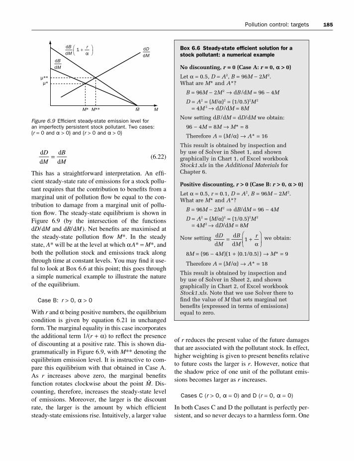
Pollution control: targets 185
(6.22)
This has a straightforward interpretation. An effi-cient steady-state rate of emissions for a stock pollu-tant requires that the contribution to benefits from amarginal unit of pollution flow be equal to the con-tribution to damage from a marginal unit of pollu-tion flow. The steady-state equilibrium is shown inFigure 6.9 (by the intersection of the functionsdD/dM and dB/dM). Net benefits are maximised atthe steady-state pollution flow M*. In the steadystate, A* will be at the level at which αA* = M*, andboth the pollution stock and emissions track alongthrough time at constant levels. You may find it use-ful to look at Box 6.6 at this point; this goes througha simple numerical example to illustrate the natureof the equilibrium.
Case B: r > 0, a > 0
With r and α being positive numbers, the equilibriumcondition is given by equation 6.21 in unchangedform. The marginal equality in this case incorporatesthe additional term 1/(r + α) to reflect the presenceof discounting at a positive rate. This is shown dia-grammatically in Figure 6.9, with M** denoting theequilibrium emission level. It is instructive to com-pare this equilibrium with that obtained in Case A.As r increases above zero, the marginal benefitsfunction rotates clockwise about the point !. Dis-counting, therefore, increases the steady-state levelof emissions. Moreover, the larger is the discountrate, the larger is the amount by which efficientsteady-state emissions rise. Intuitively, a larger value
d
d
d
d
D
M
B
M =
Figure 6.9 Efficient steady-state emission level for an imperfectly persistent stock pollutant. Two cases: r = 0 and a > 0 and r > 0 and a > 0
Box 6.6 Steady-state efficient solution for astock pollutant: a numerical example
No discounting, r == 0 (Case A: r == 0, αα >> 0)
Let α = 0.5, D = A2, B = 96M − 2M 2.What are M* and A*?
B = 96M − 2M 2 → dB/dM = 96 − 4M
D = A2 = (M/α)2 = (1/0.5)2M2
= 4M 2 → dD/dM = 8M
Now setting dB/dM = dD/dM we obtain:
96 − 4M = 8M → M* = 8
Therefore A = (M/α) → A* = 16
This result is obtained by inspection and by use of Solver in Sheet 1, and showngraphically in Chart 1, of Excel workbookStock1.xls in the Additional Materials forChapter 6.
Positive discounting, r >> 0 (Case B: r >> 0, αα >> 0)
Let α = 0.5, r = 0.1, D = A2, B = 96M − 2M 2.What are M* and A*?
B = 96M − 2M2 ⇒ dB/dM = 96 − 4M
D = A2 = (M/α)2 = (1/0.5)2M2
= 4M 2 → dD/dM = 8M
Now setting we obtain:
8M = (96 − 4M )(1 + 0.1/0.5) → M* = 9
Therefore A = (M/α) → A* = 18
This result is obtained by inspection and by use of Solver in Sheet 2, and showngraphically in Chart 2, of Excel workbookStock1.xls. Note that we use Solver there tofind the value of M that sets marginal netbenefits (expressed in terms of emissions)equal to zero.
d
d
d
d
D
M
B
M
r = +
1
α
of r reduces the present value of the future damagesthat are associated with the pollutant stock. In effect,higher weighting is given to present benefits relativeto future costs the larger is r. However, notice thatthe shadow price of one unit of the pollutant emis-sions becomes larger as r increases.
Cases C (r > 0, a = 0) and D (r = 0, a = 0)
In both Cases C and D the pollutant is perfectly per-sistent, and so never decays to a harmless form. One

186 Environmental pollution
might guess that something unusual is happeninghere by noting that equation 6.21 is undefined whenα = 0; division by zero is not a legitimate mathem-atical operation. The intuition that lies behind this isstraightforward. No steady state exists except for thecase in which M is zero. A steady state cannot existfor any positive value of M as A would rise withoutbound. But then pollution damage would also rise toinfinity.
It follows that, at some point in time, the environ-mental protection agency would have to require thatemissions be permanently set to zero to avoid theprospect of intolerable damage. The pollution stocklevel would remain at whatever level A had risen toby that time. Pollution damage would also continueindefinitely at some constant level, but no additionaldamage would be generated. The zero-emissionssteady-state solution turns out to be perfectly inaccord with good sense.
One caveat to this conclusion should be noted.Although a perfectly persistent pollutant has a zeronatural decay rate, policy makers may be able to findsome technique by which the pollutant stock may be artificially reduced. This is known as clean-upexpenditure. If such a method can be found, and can be implemented at reasonable cost, it allows thepossibility of some perpetual level of emissions. We examine this possibility further in Chapter 16.
Of course, even if the EPA accepted that emis-sions would have to be set to zero at some date (andremain zero thereafter), the question remains ofwhich date the switch to zero should be made.Steady-state analysis is unable to answer this question. To obtain that answer, another technique(or another criterion than economic efficiency) isrequired. Chapter 16 shows how optimal control canbe used to find both the efficient steady-state solu-tion and the optimal adjustment path to it.
6.10 Variable decay
The stock pollution models used in this chapter haveassumed that the proportionate rate of natural decayof the stock, α, is constant. This assumption is com-monly employed in environmental economics ana-lysis, but will not always be valid. In many situations,
one would expect that the rate of decay depend on thesize of the pollution stock, or on some other associ-ated variable. For example, it is thought that thedecay rate of greenhouse gases alters (in quite com-plex ways) as mean temperature levels change. Ofparticular importance are the existence of thresholdeffects (where the decay rate changes in a sudden,discontinuous way) and irreversibilities (where thenature of a relationship changes depending on thedirection in which a variable is moving). One ex-ample of a threshold effect is illustrated in the toppanel of Figure 6.10. Here the decay rate of a water-borne pollutant collapses towards zero as somethreshold level of biological oxygen demand (BOD)on a river is reached. This critical level of BOD isreached when the pollution stock is at M. The lowerpanel illustrates a threshold effect combined with anirreversibility. The arrows denote the direction inwhich A is changing. As the pollution stock risesfrom a low level, α collapses suddenly at the thresh-old M and remains close to zero as A continues to
Figure 6.10 Threshold effects and irreversibilities

Pollution control: targets 187
rise. At high levels of pollution, the biological abilityof the river to break down harmful pollutants mightbe largely destroyed. So if the change is reversed,and A falls from a high value, the value of α wouldremain very low (as shown by the path with left-pointing arrows). This path dependence is also knownas hysteresis; in this example, the history of pollu-tant flows matters, and reversing pollution pressuresdoes not bring one back to the status quo ex ante.
Another way of thinking about this issue is interms of carrying capacities (or assimilative capacit-ies, as they are sometimes called) of environmentalmedia. In the case of water pollution, for example, wecan think of a water system as having some capacityto transform pollutants into harmless forms. The stockpollution model of Section 6.8 has in effect assumedunlimited carrying capacities: no matter how largethe load on the system, more can always be carriedand transformed at a constant proportionate rate.
Whether this assumption is plausible is, in the lastresort, an empirical question. Where it is not, mod-elling procedures need to reflect limits to carryingcapacity. The suggestions for further reading pointyou to some literature that explores models withvariable pollution decay rates.
6.11 Convexity and non-convexity in damage and abatement cost functions
When benefit and damage functions were first pre-sented in Section 6.4, a number of assumptions weremade about their shapes. Those assumptions relateto the concept of convexity of a function. Afterexplaining what is meant by a convex function, thissection gives some examples of why the relevantfunctions may not be convex, and then shows someconsequences of non-convexity.
Consider a function, f(x), of a single variable x.The function is strictly convex if the line segmentconnecting any two distinct points on the function
lies everywhere above the function f (x), except at the two points themselves. A function is convex (asopposed to strictly convex) if the line segment lieseverywhere above or on the function f (x), but notbelow it. As an example, the function graphed inFigure 6.11 is strictly convex.
Looking back at Figure 6.4, it is clear that thedamage function D(M) is convex.15 This is not truefor the benefits function B(M) as that is drawn inFigure 6.4. However, suppose that we reinterpretbenefits as avoided abatement costs, as suggestedearlier. Now construct the horizontal image of B(M),so that moving to the right on this mirror image corresponds to more pollution abatement. Then theabatement cost function will be convex.
Actually, this terminological contortion is notreally necessary. What really matters, as we shallsee, is whether the functions describing the problembeing investigated are smooth, continuous, and leadto unique marginal efficient conditions. All of theseproperties are satisfied by the benefit and damagefunctions used in Figure 6.4. It is clear from thelower panel of Figure 6.4 that there is just one levelof pollution at which the marginal efficiency condi-tion is satisfied: the marginal benefit of pollution (orequivalently marginal cost of abatement) is equal tothe marginal damage of pollution. This implies thatmarginal analysis alone is sufficient for identifyingthe efficient level of pollution.16
Figure 6.11 A strictly convex function
15 In fact, as drawn it is strictly convex. But what matters iswhether the weaker property of convexity is satisfied. So we shalluse the word ‘convex’ from now on to cover strict as well as (weak)convexity.
16 Mathematically, the efficient pollution level is obtained from the first-order conditions for optimisation; second-order condi-tions will automatically be satisfied (and so do not need to bechecked).

188 Environmental pollution
6.11.1 Non-convexity of the damage functionand its implications
There are many reasons why the damage functionand the abatement cost function may be non-convex.Here we restrict attention to the more commonly dis-cussed case of non-convex damages. So what mightcause a pollution damage function to not be of thesmooth, continuously increasing form that we haveassumed so far? One example was given implicitlyin Section 6.10 where we introduced the ideas ofthreshold effects and irreversibility. A closely relatedexample to that is acidic pollution of rivers andlakes. Here, pollution may reach a threshold point atwhich the lake become biologically dead, unable tosupport animal or plant life. No further damage isdone as pollution levels rise beyond that point. Thetotal and marginal damages function in this case willbe of the form shown in Figure 6.12.
Another example, discussed in Fisher (1981), isnon-convexity of damages arising from avertingbehaviour by an individual. Suppose a factory emitsparticulate emissions that create external damagesfor an individual living in the neighbourhood of thefactory. The marginal damage initially rises with theamount of the pollution. However, at some critical
level of pollution flow, the affected individual canno longer tolerate living in the neighbourhood of thefactory, and moves to live somewhere else where thedamage to him or her becomes zero. As far as thisparticular individual is concerned, their marginaldamage function is also of the form shown in Figure6.12. However, if there are many individuals livingin the neighbourhood, with varying tolerance levels,many of whom are prepared to move at some levelof pollution, the aggregate marginal pollution dam-age function will be the sum of a set of individualfunctions, each of which has the same general formbut with differing pollution tolerance levels. Theaggregate damage function will be of the non-convex form shown in the top panel of Figure 6.13,with its marginal counterpart being shown by thecurve labelled MD in the central panel.
Now combine the marginal damage function forthe averting behaviour example with a marginalbenefit function of conventional shape. This isshown in the central panel of Figure 6.13. Marginaldamage and benefits are equalised here at threeemission levels. To ascertain which of these, if any,is the efficient level of pollution, it is necessary toinspect the level of total net benefits at these threepoints, and at all other levels of emission (as netbenefits will not necessarily even correspond to amarginal equality when one or more function is not convex). The two points labelled A and B are‘local optima’, as they satisfy the second-order con-ditions for a local maximum of net benefits, asshown in the lower panel of Figure 6.13. In this caseit can be seen by inspection of the NB curve that M3
is a ‘global’ net benefits-maximising pollution level.Note that in moving from M1 to M3, net benefits atfirst fall (by the area labelled a) and then rise (by thearea labelled b).
Why does non-convexity matter? There are twomajor reasons why this is a matter of concern. Thefirst could be described as a ‘practical’ matter: cal-culating the efficient level of emissions (or pollutionstock) is likely to be more complicated than where all functions are convex. This is partly a matter of computational difficulty. But more importantly, it is to do with the fact that the information required to identify the (non-convex) functions maybe immense and very costly to obtain. Obtaining
Figure 6.12 A non-convex damage function arising frompollution reaching a saturation point
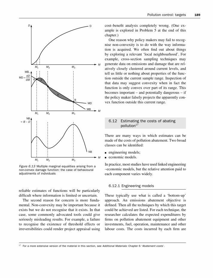
Pollution control: targets 189
reliable estimates of functions will be particularlydifficult where information is limited or uncertain.
The second reason for concern is more funda-mental. Non-convexity may be important because itexists but we do not recognise that it exists. In thatcase, some commonly advocated tools could giveseriously misleading results. For example, a failureto recognise the existence of threshold effects orirreversibilities could render project appraisal using
cost–benefit analysis completely wrong. (One ex-ample is explored in Problem 5 at the end of thischapter.)
One reason why policy makers may fail to recog-nise non-convexity is to do with the way informa-tion is acquired. We often find out about things by exploring a relevant ‘local neighbourhood’. Forexample, cross-section sampling techniques maygenerate data on emissions and damage that are rel-atively closely clustered around current levels, andtell us little or nothing about properties of the func-tion outside the current sample range. Inspection ofthat data may suggest convexity when in fact thefunction is only convex over part of its range. Thisbecomes important – and potentially dangerous – ifthe policy maker falsely projects the apparently con-vex function outside this current range.
6.12 Estimating the costs of abating pollution17
There are many ways in which estimates can bemade of the costs of pollution abatement. Two broadclasses can be identified:
n engineering models;n economic models.
In practice, most studies have used linked engineering–economic models, but the relative attention paid toeach component varies widely.
6.12.1 Engineering models
These typically use what is called a ‘bottom-up’approach. An emissions abatement objective isdefined. Then all the techniques by which this targetcould be achieved are listed. For each technique, theresearcher calculates the expected expenditures byfirms on pollution abatement equipment and otherinvestments, fuel, operation, maintenance and otherlabour costs. The costs incurred by each firm are
Figure 6.13 Multiple marginal equalities arising from anon-convex damage function: the case of behaviouraladjustments of individuals
17 For a more extensive version of the material in this section, see Additional Materials: Chapter 6 ‘Abatement costs’.

190 Environmental pollution
then added up to arrive at the total economy-wideabatement cost. Hence the name ‘bottom-up’. For acomplete accounting of control costs, expendituresincurred by regulatory agencies should be added in.Best achievable abatement costs are those which arethe minimum among those techniques studied. Amore modest variant of this approach would involvethe researcher obtaining cost estimates of one tech-nique rather than all available. This requires makingassumptions about the form of responses of firms tothe controls they face.
There are some desirable properties in estimatingabatement costs in this way. They are simple tounderstand, and simple (at least in principle) toundertake. Engineering models are typically highlydisaggregated. They consider technology options in a rich, detailed way, providing large amounts of information at the micro-production level. Thistechnology-rich property means that engineeringmodels are very well suited to costing specific pro-jects, such as using wind power to generate 25% ofa country’s electricity. They are also capable of dealing in a careful way with some kinds of ‘no-regret’ or ‘free-lunch’ possibilities arising from tech-nical and economic inefficiencies in existing methodof production. (See Box 6.3 for more details.)
But this approach also has some serious limita-tions. Each technology is assessed independently via an accounting of its costs and savings, but pos-sible interdependencies (or linkages and feedback)between the elements being studied and the economyas a whole are not taken into account. This leads to biased estimates of the true costs of abatement.Some examples of important linkages that matter –but which are typically ignored by engineering models – are:
n productivity changes induced by regulatorycontrol;
n changes in unemployment;n change in overall industrial structure of the
economy.
The most fundamental problem is that engineeringmodels ignore changes in relative prices, and theassociated impacts on factor substitution and the
behaviour of firms and individuals. Results can beseriously misleading because of this, particularlywhen long-term effects are being investigated.
6.12.2 Economic models
These are typically ‘top-down’ models.18 They areconstructed around a set of aggregate economic vari-ables, the relationships among which are determinedby (micro or macro) economic theory and equilib-rium principles. These relationships are estimatedeconometrically, using time-series data. Alternat-ively, relationships are calibrated to match with datafor one chosen base year. To obtain cost estimates,some project of interest such as the introduction of a carbon tax is taken as an exogenous shock. Themodel is solved for equilibrium before and after the shock. By comparing the values of relevant variables in the baseline and shocked case, cost estimates are obtained.
The top-down nature of these models means thatthey tend to be highly aggregated, and that they donot have the richness of detail (particularly aboutenergy technology options) that can be captured in engineering models. The strength of economicmodels lies in their ability to deal with supply anddemand relationships, and to capture behaviouralchanges and substitution effects that are importantfor making inferences about long-term con-sequences. In addition, they are good for the ana-lysis of distributional effects, and for simulating theuse of economic instruments.
But economic models alone treat the energy sec-tor as a relatively undifferentiated whole, and so areof limited use for answering questions that involvechanges within the energy sector. Aggregate output–energy use relationships tend to be relativelyinflexible, and so economic models are not wellsuited to examining possible decoupling effects.One major practical limitation of economic modelsis their assumption that resource allocation in thebaseline case is already fully efficient. As a result,they can say nothing about negative cost potentialfrom removing existing inefficiencies.
18 See IPCC(3) (2001) for further analysis of bottom-up and top-down models.

Pollution control: targets 191
Economic models typically yield higher abate-ment cost estimates than engineering models. Thisarises because (a) they do not consider existinginefficiencies and (b) they take account of losses ofconsumer surplus arising from price increases asregulated firms attempt to pass additional costs on toconsumers.
6.12.3 Linked or integratedengineering–economic models
Ideally, one would like to base cost estimates onmodels that combine the advantages of economicand engineering models. This might be done by link-ing the two, or by more systematically developingan integrated modelling approach. Among the manyattempts that have been made to do this, we find thefollowing types.
6.12.3.1 Input–output (IO) models
IO models (see Chapter 9 for a more developedaccount) partition the economy into a number of sec-tors, and then represent the economy mathematicallyby a set of simultaneous linear equations. Theseequations embody the input–output relationshipsbetween those sectors. IO models, therefore, capturesectoral interdependences and spillovers. So, forexample, if the use of coal were to be reduced, IOmodels could explore the ramifications of this for theeconomy as a whole, and so give some idea aboutthe likely costs. However, the fixed coefficients inthe IO equations preclude modelling of behaviouralchanges and factor substitution effects as relativeprices change. Hence, they will tend to overestimateabatement costs. IO models are useful for short-runmodelling where disaggregated sectoral detail isrequired.
6.12.3.2 Macroeconomic models
Macroeconomic models give a key role to changesin effective demand and investigate the resultingquantity changes. More sophisticated models alsoincorporate overall wage and price-level changes,and describe the dynamics of, and adjustment to,
new equilibria as a result of shocks. When thesemodels are linked with others that deal more richlywith the energy sector, they can be useful for invest-igating the short-run and medium-term cost implica-tions of environmental policy changes.
6.12.3.3 Computable general equilibrium (CGE) models
CGE models (see Chapter 9 for more details) simu-late the behaviour of agents based on optimisingmicroeconomic theory. The models are solved forsets of prices and wages that generate general equi-librium. CGE models are typically static models,and do not analyse adjustment processes from oneequilibrium state to another. They are widely used tosimulate the consequences of emissions taxes.
6.12.3.4 Dynamic energy optimisation models
These are ‘bottom-up’, technology rich, partial equilibrium energy-sector models. They are used to minimise cost of the energy sector over a long-term horizon, yielding a partial equilibrium forenergy markets. Sophisticated versions allow energydemand to respond to price, and examine the dyn-amics of changes in the energy sector (and so cantrace out the evolution through time of changes inthe size and type of capital stock used in the energysector. Energy optimisation models are often linkedwith macro models.
6.12.3.5 Purpose-built integrated energy–economic system simulation (E–E) models
E–E models are usually purpose-built to estimateabatement costs in one particular context (such asthe costs of abatement required to attain KyotoProtocol targets for greenhouse gases). They are bottom-up representations of energy demand andsupply technologies, and as such typically have avery rich specification of technologies at a highlydisaggregated level. A purpose-built economic com-ponent is constructed that is consistent with theenergy structure of the model. E–E models are oftenused to simulate the consequences (and costs) ofvarious scenarios.
In practice, most E–E models are hybrids, withproblems of inconsistency between components. For

192 Environmental pollution
Box 6.7 IPCC estimates of the costs of CO2 abatement to reach Kyoto Protocol targets
The gross abatement costs to attain Kyoto targetsfor carbon dioxide reduction depend on severalfactors:
1. The magnitude of emissions reductionrequired to meet the target. Assumptionsmade about marginal sources of supply (cost and availability of carbon-based andcarbon-free technologies)
2. Short- and long-run price elasticities3. Whether or not there is emissions trading
(and how extensive this is)
Point 1 implies that the emissions ‘baseline’ is critical to the magnitude of total abatementcosts. The larger emissions growth would be inthe absence of control, the higher will be totalabatement costs required to attain the Kyototarget. Emissions baseline growth rate of CO2
depends on GDP growth, the rate of decline ofenergy per unit output, and the rate of decline ofCO2 emissions per unit energy.
The net costs depend on the gross costs andalso on
1. Availability of no-regrets efficiency gains (e.g.can revenues be used to reduce marginal rateson other distortionary taxes – such as income,sales, or employment taxes – or reduce othertechnical/economic inefficiencies?)
2. Whether abatement will generate otherancillary benefits
3. The magnitude of any induced technicalprogress. Of importance here, in terms of thetiming of costs, is whether the innovationroute is via R&D or learning-by-doing.
Working Group III of the IntergovernmentalPanel on Climate Change (IPCC) of the UnitedNations commissioned a number of independentmodelling groups to simulate emissionsreductions achieved by carbon taxes. Each of these groups employed some variant ofenergy–economy model. Tax revenues wererecycled via lump-sum payments to the wholeeconomy. The value of the tax rate required to achieve an emissions target indicates themarginal abatement cost in that model. Witheach team using different assumptions aboutbaseline emissions and different modelstructures and/or parameter values, the exerciseallows multi-model comparisons to be made, and the sensitivity of findings to variations inassumptions can be explored.
The estimated marginal abatement costs fromthese various models for attaining Kyoto Protocoltargets by 2010 are shown in Table 6.5. Figuresare given for three scenarios. The first scenario isone in which no trading of allowances is allowed
Table 6.5 Marginal abatement costs (1990 US$/tC) for attainment of Kyoto target by 2010
Model No trading Annex 1 trading Global trading
US OECD-Europe Japan CANZ
ABARE-GTEM 322 665 645 425 106 23AIM 153 198 234 147 65 38CETA 168 46 26Fund 14 10G-Cubed 76 227 97 157 53 20GRAPE 204 304 70 44MERGE3 264 218 500 250 135 86MIT-EPPA 193 276 501 247 76MS-MRT 236 179 402 213 77 27RICE 132 159 251 145 62 18SGM 188 407 357 201 84 22WorldScan 85 20 122 46 20 5Administration 154 43 18EIA 251 110 57POLES 135.8 135.3 194.6 131.4 52.9 18.4
Source: IPCC(III) 2001, Table TS.4, p. 56One set of results (Oxford) has been omitted from this table, as it had not been fully reviewed at the time of writing,and relied on early 1980s data for initial parameterisation.Models do not take account of induced technical progress, Clean Development Mechanism, sinks, negative cost options,targeted recycling of revenues, ancillary benefits, inclusion of non-CO2 gases, or inefficiencies in implementation.Models here are typically general equilibrium rather than bottom-up technology-rich models.

Pollution control: targets 193
example, one may have as its basis a sophisticatedengineering model that can be used to calculate dir-ect technical costs. Linked to this might be a modulewhich uses observed market behaviour to estimatetechnology adaptations. Further components estim-ate welfare losses due to demand reductions, and therevenue gains and losses due to trade changes.
6.13 Choosing pollution targets on grounds other than economic efficiency
This chapter has been largely concerned with pollu-tion targets set in terms of an economic efficiencycriterion. But there are (at least) two reasons whythis focus is unduly restrictive. First, in the contextof limited or imperfect information, there may beimmense difficulties in identifying economicallyefficient targets.19 In that case, efficiency-based tar-gets may be of theoretical interest only and have little practical significance. We examine this issue atsome length in Chapter 8.
Second, policy makers are likely to have multipleobjectives. Efficiency matters, but it is not the onlything that matters. It is not surprising, therefore, that
targets (or ‘environmental standards’ as they aresometimes called) are often chosen in practice on thebasis of a mix of objectives. The mix may includehealth or safety considerations, equity, and percep-tions of what is technically feasible (usually subjectto some ‘reasonable cost’ qualification). In recentyears, sustainability has taken its place as anotherstated goal of policy. As we show in Chapter 8, sustainability in conjunction with imperfect informa-tion and uncertainty may also point to some form ofprecautionary principle being incorporated in the setof objectives pursued by policy makers.
National and international policy is also deter-mined in the context of a network of pressures andinfluences. It is not surprising, therefore, that polit-ical feasibility plays a significant role. This has beenparticularly important in the area of internationalenvironmental agreements over such things as ozonedepletion, acid rain and the greenhouse effect, as weshow in Chapter 10.
Tables 6.6 and 6.7 list some existing environ-mental standards and the criteria that appear to havebeen used in their selection. In the next chapter weinvestigate which instruments are available to anenvironmental protection agency for attaining agiven pollution target, however that target may havebeen determined.
19 Many of the problems posed by imperfect information also applyto targets set on the basis of sustainability, health, or indeed anyother criterion. Nevertheless, they apply particularly strongly toefficiency-based targets. However, as we shall see in the following
chapter, several of the alternative criteria can be interpreted asappropriate for target setting precisely when information is imper-fect. They should then be thought of as responses to uncertaintyrather than as being weakened or limited by it.
between countries – each country mustindependently achieve the emission target for it specified in the Protocol (see Chapter 10 fordetails of these targets). In this case, marginalabatement costs are shown for four ‘blocs’ of countries. It is evident that the marginalabatement costs vary considerably overcountries, implying that the total globalemissions reduction is not being achieved at least cost.
A second scenario allows trading of allowances(permits) among the Annex 1 countries (roughlyspeaking, the industrialised economies). Noticehow partial trading dramatically reducesmarginal (and so total) abatement costs. This is even more evident in results for the thirdscenario in which trading can take place betweenany countries. The efficiency gains that thisgenerates mean that marginal costs are reducedby around an order of magnitude (a tenfoldreduction) in some cases.
Box 6.7 continued

Summary
n We do not expect pure market economies to deliver efficient outcomes in terms of pollution.Pollution tends to be an externality to the market process and as a result is not adequately reflectedin private market decisions. Put another way, while firms would meet the costs of controlling orabating pollution, the benefits of abatement would not be received by firms (although they wouldby society). Hence, in considering pollution abatement, the control level that maximises netbenefits to firms is different from the level that maximises social net benefits.
n Economists often recommend that pollution targets should be set using an economic efficiencycriterion. This can be thought of as selecting pollution targets so as to maximise social net benefits
n Economic efficiency is not the only relevant criterion for pollution target setting. Several otherswere discussed in the chapter. Which criteria are important to policy makers will tend to reflecttheir policy objectives and the constraints under which they operate.
194 Environmental pollution
Table 6.7 Primary NAAQS for Criteria Air Pollutants, 1997
Concentration level
Pollutant Averaging time ppm µg/m3
Particulate matter (PM10) Annual – 5024-hour – 150
Particulate matter (PM2.5) Annual – 1524-hour – 65
Sulphur dioxide Annual 0.030 8024-hour 0.140 365
Carbon monoxide 8-hour 9.000 101-hour 35.000 40
Nitrogen oxide Annual 0.053 100Ozone 8-hour 0.008 –Lead Max. quarterly – 1.5
Table 6.6 Environmental targets
Pollutant
United KingdomGrains emitted in cement productionSewage concentration
Cadmium/lead
PCBsWaste recycling
United StatesCriteria air pollutants
InternationalCFCs
Key: BOD = biochemical oxygen demand. The concepts of ‘Best practicable means’, ‘Critical load’, and ‘Precautionary principle’ areexplained elsewhere in the chapter
Relevant criterion
Best practicable means
1976 National Water Council: precautionaryprinciple, perceived health risksHealth criterion
Strict precautionary principle – health risksPolitical target?
Health risks
Political feasibility, with final targets set interms of critical load
Target
0.1–0.2 grains per cubic foot
Max. 30 mg/litre suspended solidsMax. BOD 20 mg/litreDischarges into North Sea to fall by 70% between1985 and 1995Phase out by 199950% domestic waste to be recycled
See Table 6.7
CFC production to fall to 80% and 50% of 1986levels by 1994 and 1999 respectively

Pollution control: targets 195
n There are important differences between flow pollutants and stock pollutants in terms of themechanisms by which damage is generated. This distinction has implications for the way in whichtargets are derived using an economic efficiency criterion. For stock pollutants, persistence impliesthat attention must be given to the accumulation (and decay) of pollutants over time, and so anintertemporal analysis is required. This is not necessary for the analysis of flow pollutants.
n For long-lived stock pollutants, pollution targets are best thought of in terms of emissions pathsover time. Efficient pollution paths will not in general imply the same level of control at all pointsin time. However, it is often useful to think of steady-state outcomes and to investigate what(constant) level of pollution control would be efficient in an equilibrium steady state.
n Where a stock pollutant is not uniformly mixing, the spatial distribution of emissions sourcesbecomes relevant. If targets are set in terms of pollutant concentrations, then the allowableemissions of any particular source will depend on its location.
Further reading
ticularly chapter 8. More advanced references areLaffont and Tirole (1993) which discusses theoriesof regulation, and Stigler (1971) and Peltzman(1976); these last two references are seminal workson the interest group theory of regulation.
Grubb (1998) provides a very interesting accountof greenhouse gas policy, focusing on technologicalresponses to the Kyoto Protocol. Ulph (1997) con-siders the relationship between environmental policyand innovation. Porter (1991) articulates the argumentthat strict environmental policy may be a factorwhich stimulates the rate of technological innova-tion. The double dividend hypothesis is discussed byBovenberg (1997). The collection of readings editedby Carraro and Siniscalco (1997) focuses on the ap-plication of game theory to environmental problems.This is a particularly useful tool in the analysis ofinternational pollution problems, as we shall see inChapter 10, but has interesting applications too fordomestic pollution policy. One of the first studiesabout the difficulties in designing optimal taxes (andstill an excellent read) is Rose-Ackerman (1973).
Some journals provide regular applications of theeconomic theory of pollution. Of particular interestare the Journal of Environmental Economics andManagement, Ambio, Environmental and ResourceEconomics, Land Economics, Ecological Modelling,Marine Pollution Bulletin, Ecological Economicsand Natural Resources Journal.
Excellent and extensive presentations of the eco-nomics of pollution are to be found in Fisher (1981,chapters 5 and 6), Anderson (1985, 1991), Hartwickand Olewiler (1986, 1998) and Kolstad (2000).Baumol and Oates (1988) is a classic source in thisarea, although the analysis is formal and quite diffi-cult. Cornes and Sandler (1996) provides a powerfultheoretical underpinning in terms of the theory ofpublic goods.
Tietenberg (1992) gives very extensive, descript-ive coverage of several specific types of pollution.Other useful treatments which complement the dis-cussion in this chapter are Dasgupta (1982, chapter8), and two survey articles by Fisher and Peterson(1976) and Cropper and Oates (1992). Smith (1972)gives a mathematical presentation of the theory ofwaste accumulation. Several excellent articles canbe found in the edited volume by Bromley (1995).
In this chapter we have taken a ‘normative’approach to the setting of pollution targets, analys-ing what such targets should be in terms of some criterion of the public interest. An alternative liter-ature considers targets in ‘positive’ terms, dealingwith how targets are actually set. This approachfocuses on the behaviour of interest groups, attempt-ing to gain rents by manipulating government policyto their advantage. Good introductory accounts ofthis ‘political economy’ of regulation can be foundin Goodstein (1995, 1999) and Kolstad (2000), par-
196 Environmental pollution
Discussion questions
private gain will always be the enemy of a cleanenvironment.’ Examine this proposition.
3. Discuss the relevance and application of theconcept of externalities in environmentaleconomics.
1. ‘Only the highest standards of environmentalpurity will do.’ Discuss.
2. ‘A clean environment is a public good whosebenefits cannot be privately appropriated.Therefore private industry which is run for
Problems
1. Under which circumstances will theeconomically optimal level of pollution be zero?Under which circumstances will it be optimal toundertake zero pollution abatement?
2. We have seen that the efficient level of pollution is the one that minimises the sum oftotal abatement costs plus total damage costs. Refer now to Figure 6.5. Show that if pollutionabatement takes place to the extent ! − MA thesum of total damage costs and total abatementcosts is C1 + C2 + C3. Prove that ‘too little’abatement (relative to the optimal quantity)results in higher costs than C1 + C2.
3. Explain the concept of the ‘efficient level ofpollution’. What information is required in orderto identify such an efficient quantity?
4. Using equation 6.20 or 6.21, deduce the effectof (i) a decrease in α and (ii) an increase in r(ceteris paribus) on:(a) M*(b) A*(c) µ*
Note that you could answer this questionanalytically. Alternatively, you could explorethe issue numerically using the Excel file
Stock1.xls (found in the Additional Materialsfor Chapter 6).
5. This problem illustrates how marginal analysismight give misleading results in the presence of non-convexity. It is based on an examplefrom Goodstein (1995). Nitrogen oxides (NOx),in combination with some volatile organiccompounds and sunlight, can produce damaginglower-atmosphere ozone smog. Initially, thedamage rises at an increasing rate with NOx
emissions. However, high levels of NOx act asozone inhibitors, and so beyond some criticallevel of emissions, higher levels of NOx reduceozone damage.(i) Sketch a marginal damage (MD) function
that is consistent with these properties.(ii) Add to your diagram a conventionally
shaped marginal benefits function (ormarginal abatement cost function) thatintersects the MD function in more thanone place.
(iii) By an appropriate choice of some initiallevel of emissions, demonstrate that thefollowing rule may give misleading results.Rule: emissions should be increased(decreased) if a small increase in emissionsincreases (decreases) net benefits.
Appendix 6.1 Matrix algebra
A6.1.1 Introduction
In this chapter, and in a few of the later ones (par-ticularly Chapter 9 and the appendix to Chapter 14),some use is made of matrix algebra notation and ele-
mentary matrix operations. This appendix provides,for the reader who is unfamiliar with matrix algebra,a brief explanation of the notation and an expositionof a few of its fundamental operations. We deal hereonly with those parts of matrix algebra that are

Pollution control: targets 197
necessary to understand the use made of it in thistext. The reader who would like a more extensiveaccount should go to any good first-year university-level mathematics text. For example, chapter 4 ofChiang (1984) provides a relatively full account ofintroductory-level matrix algebra in an accessibleform.
A6.1.2 Matrices and vectors
A matrix is a set of elements laid out in the form ofan array occupying a number of rows and columns.Consider an example where the elements are num-bers. Thus, the array of numbers
0.7 0.10.9 0.20.3 0.20.1 0.0
can be called a matrix. In such an array, the relativepositions of the elements do matter. Two matricesare identical if the elements are not only the samebut also occupy the same positions in each matrix. Ifthe positions of two or more elements were inter-changed, then a different matrix would result (unlessthe interchanged elements were themselves identical).
It is conventional, for presentational purposes, toplace such an array within square brackets, and tolabel the matrix by a single bold letter (usuallyupper-case).20 So in the following expression, A isthe name we have given to this particular matrix ofeight numbers.
It is also conventional to define the dimension of amatrix by the notation m × n where m is the numberof rows occupied by the elements of the matrix andn is the number of columns occupied by elements ofthe matrix. So, for our example, A is of dimension 4× 2 as its elements span four rows and two columns.
Notice that because elements of matrices spanrows and columns, they can be handled very con-veniently within spreadsheet programs.
A
. .
. .
. .
. .
=
0 7 0 10 9 0 20 3 0 20 1 0 0
Sometimes we want to define a matrix in a moregeneral way, such that its elements are numbers, butthose numbers are as yet unspecified. To do this wecould write A in the more general form
Notice the way in which each of the elements of thismatrix has been labelled. Any one of them is aij
where i denotes the row in which it is found and j denotes its column. With this convention, the bottom right element of the matrix – here a42 – willnecessarily have a subscript identical to the dimen-sion of the matrix, here 4 × 2.
It is convenient to have another shorthand nota-tion for the matrix array. This is given by
i = 1, . . . , mA = [aij] j = 1, . . . , n
The bracketed term here lets the reader know thatwhat is being referred to is a matrix with m × nelements aij.
A6.1.2.1 A special form of matrix: the identity matrix
A matrix is said to be square if its row and columndimensions are equal (it has the same number ofrows and columns). Thus, the matrix
is a 2 × 2 square matrix. Furthermore, if the co-efficients of a square matrix satisfy the restrictionsthat each element along the leading (top left to bot-tom right) diagonal is 1 and every other coefficientis zero, then that matrix is called an identity matrix.Thus the matrix
is a 2 × 2 identity matrix. An identity matrix is often denoted by the symbol I, or sometimes by In
I =
1 00 1
B =
3 24 1
A =
a aa aa aa a
11 12
21 22
31 32
41 42
20 The use of square brackets is not universal; some authors prefer round brackets or braces.

198 Environmental pollution
where the n serves to indicate the row (and column)dimension of the identity matrix in question. In ourexample, it would be I2.
A6.1.2.2 Vectors
A vector is a special case of a matrix in which allelements are located in a single row (in which caseit is known as a row vector) or in a single column(known as a column vector). Looking at the variousrows and columns in the 4 × 2 matrix A above, it isevident that we could make up six such vectors fromthat matrix. We could construct four row vectorsfrom the elements in each of the four rows of thematrix. And we could make up two column vectorsfrom the elements in each of the two columns.21 Thefour row vectors constructed in this way are
[a11 a12] [a21 a22] [a31 a32] and[a41 a42]
each of which is of dimension 1 × 2, while the twocolumn vectors, each of dimension 4 × 1, are givenby
A6.1.2.3 The transpose of a matrix or a vector
Various ‘operations’ can be performed on mat-rices.22 One of the most important – and commonlyused – is the operation of forming the ‘transpose’ ofa matrix. The transpose of a matrix is obtained byinterchanging its rows and columns, so that the firstcolumn of the original matrix becomes the first rowof the transpose matrix, and so on. Doing thisimplies that if the original matrix A were of dimen-sion m × n, its transpose will be of dimension n × m.The transpose of A is denoted as A′, or sometimes as AT.
Consider two examples. First, let a be the 4 × 1column vector
aaaa
aaaa
11
21
31
41
12
22
32
42
and
then its transpose, a′′ is given by the row vector a′′ = [a11 a21 a31 a41].
As a second example, consider the first array thatwe introduced in this appendix. That matrix and itstranspose are given by
A6.1.2.4 Bold notation for vectors and matrices
As we mentioned earlier, it is conventional to usethe bold font to denote vectors or matrices, and touse an ordinary (non-bold) font to denote a scalar(single number) term. Hence, in the followingexpression, we can deduce from the context and thenotation employed that each of a1 and a2 is a columnvector consisting respectively of the first column ofscalars and the second column of scalars. We knowthat the element a21, for example, is a scalar becauseit is not written in bold font.
A6.1.3 Other operations on matrices
As with algebra more generally, several operationssuch as addition and multiplication can, under someconditions, be performed on matrices.
A6.1.3.1 Addition and subtraction
Two matrices can be added (or subtracted) if theyhave the same dimension. Essentially, these operations
A a a1 2 [ ]=
=
a aa aa aa a
11 12
21 22
31 32
41 42
A A
. .
. .
. .
. .
. . . .. . . .
=
=
0 7 0 10 9 0 20 3 0 20 1 0 0
0 7 0 9 0 3 0 10 1 0 2 0 2 0 0
′′
a =
aaaa
11
21
31
41
21 One could also, of course, make up other vectors as mixturesof elements from different rows or columns.
22 From this point on in this appendix, we shall use the term matrixto include both vectors and matrices, unless the context requiresthat we distinguish between the two.
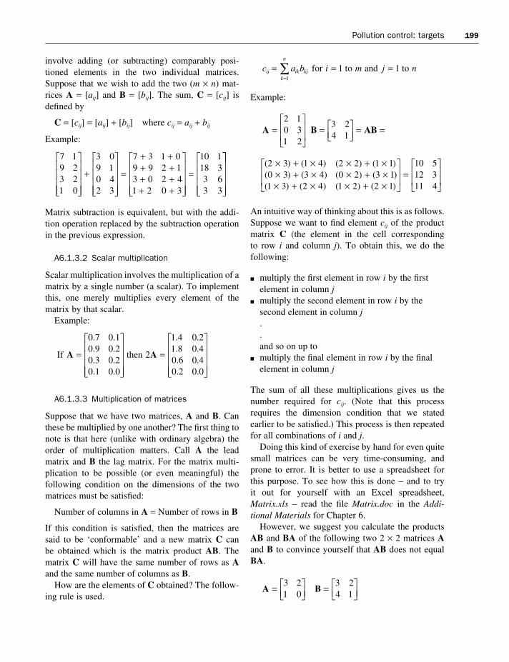
Pollution control: targets 199
involve adding (or subtracting) comparably posi-tioned elements in the two individual matrices.Suppose that we wish to add the two (m × n) mat-rices A = [aij] and B = [bij]. The sum, C = [cij] isdefined by
C = [cij] = [aij] + [bij] where cij = aij + bij
Example:
Matrix subtraction is equivalent, but with the addi-tion operation replaced by the subtraction operationin the previous expression.
A6.1.3.2 Scalar multiplication
Scalar multiplication involves the multiplication of amatrix by a single number (a scalar). To implementthis, one merely multiplies every element of thematrix by that scalar.
Example:
A6.1.3.3 Multiplication of matrices
Suppose that we have two matrices, A and B. Canthese be multiplied by one another? The first thing tonote is that here (unlike with ordinary algebra) theorder of multiplication matters. Call A the leadmatrix and B the lag matrix. For the matrix multi-plication to be possible (or even meaningful) the following condition on the dimensions of the twomatrices must be satisfied:
Number of columns in A = Number of rows in B
If this condition is satisfied, then the matrices aresaid to be ‘conformable’ and a new matrix C can be obtained which is the matrix product AB. Thematrix C will have the same number of rows as Aand the same number of columns as B.
How are the elements of C obtained? The follow-ing rule is used.
If then
. .
. .
. .
. .
. .
. .. .. .
A A=
=
0 7 0 10 9 0 20 3 0 20 1 0 0
2
1 4 0 21 8 0 40 6 0 40 2 0 0
7 19 23 21 0
3 09 10 42 3
7 3 1 09 9 2 13 0 2 41 2 0 3
10 118 33 63 3
+
=
+ ++ ++ ++ +
=
Example:
An intuitive way of thinking about this is as follows.Suppose we want to find element cij of the productmatrix C (the element in the cell corresponding to row i and column j). To obtain this, we do the following:
n multiply the first element in row i by the firstelement in column j
n multiply the second element in row i by thesecond element in column j..and so on up to
n multiply the final element in row i by the finalelement in column j
The sum of all these multiplications gives us thenumber required for cij. (Note that this processrequires the dimension condition that we stated earlier to be satisfied.) This process is then repeatedfor all combinations of i and j.
Doing this kind of exercise by hand for even quitesmall matrices can be very time-consuming, andprone to error. It is better to use a spreadsheet forthis purpose. To see how this is done – and to try it out for yourself with an Excel spreadsheet,Matrix.xls – read the file Matrix.doc in the Addi-tional Materials for Chapter 6.
However, we suggest you calculate the productsAB and BA of the following two 2 × 2 matrices Aand B to convince yourself that AB does not equalBA.
A B =
=
3 21 0
3 24 1
( ) ( ) ( ) ( )( ) ( ) ( ) ( )( ) (
× + × × + ×× + × × + ×× + ×
2 3 1 4 2 2 1 10 3 3 4 0 2 3 11 3 2 ) ( ) ( )
4 1 2 2 1
10 512 311 4× + ×
=
A B AB =
=
= =2 10 31 2
3 24 1
c a b i m j nij ik kjk
n
= = ==
∑ 1
1 1for to and to

200 Environmental pollution
A6.1.3.4 Division
Whereas obtaining the product of two matrices is ameaningful operation in matrix algebra, and can bedone providing the two matrices are ‘conformable’,the same cannot be said of matrix division. Indeed,the division of one matrix by another is not a mean-ingful operation.
A6.1.3.5 The inverse matrix
However, a related concept – matrix inversion –does exist and is fundamental to much that is done inmatrix algebra. To motivate this concept, think ofordinary algebra. If a and b are two numbers then thedivision of a by b (i.e. a/b) can be done, providedthat b is non-zero. But notice that a/b can also bewritten as ab−1, where b−1 is the inverse (or recip-rocal of b).
Where B is a matrix, we can under some condi-tions obtain its inverse matrix, B−1. And if we have asecond matrix, say A, which has the same number ofrows as B−1 has columns, then the product B−1A canbe obtained.
How is the inverse of B defined? The matrixinverse must satisfy the following equality:
BB−1 == B−1B == I
That is, the product of a matrix and its inverse matrixis the identity matrix. Inspecting the dimension con-ditions implied by this definition shows that a matrixcan only have an inverse if it is a square matrix.
Let us look at an example. The inverse of the matrix
is given by
as
We will not give any methods here by which aninverse can be obtained. There are many such rules,all of which are tedious or difficult to implementonce the matrix has more than 3 rows. Instead, we
0 10 5 1 5
3 21 0
3 21 0
0 10 5 1 5
1 00 1. .
. .
−
=
−
=
A− = −
1 0 10 5 1 5
. .
A =
3 21 0
just report that a modern spreadsheet package canobtain inverse matrices by one simple operation,even for matrices of up to about 70 rows in size.There is clearly no need to bother about deriving aninverse by hand! And, of course, it is always pos-sible to verify that the inverse is correct by check-ing that its product with the original matrix is I.
Once again, to see how this is done, seeMatrix.doc and Matrix.xls.
A6.1.4 The uses of matrix algebra
The two main uses we make of matrix algebra in thistext are
n to describe a system of linear equations in acompact way;
n to solve systems of equations or to carry outrelated computations.
Each of these is used in this chapter (in Section 6.8,where we discuss ambient pollution standards) andin Chapter 9. As an example of the first use, it is evident that the system of equations used in ourambient pollution example,
A1 = d11M1 + d12M2
A2 = d21M1 + d22M2
A3 = d31M1 + d32M2
A4 = d41M1 + d42M2
can be more compactly written as A == DM
where
Check for yourself that, after the matrix multiplica-tion DM, this reproduces the original system of fourequations.
The potential power of matrix algebra as a com-putational or solution device is illustrated in ouranalysis of input–output analysis in Chapter 9. Wewill leave you to follow the exposition there. As youwill see, it is in this context that the inverse of amatrix is useful.
D M A =
=
=
d dd dd dd d
MM
AAAA
11 12
21 22
31 32
41 42
1
2
1
2
3
4

Pollution control: targets 201
Appendix 6.2 Spatially differentiated stock pollution: a numerical example
which gives:
a − bM1 = d11(d11M1 + d12M2) + d21(d21M1 + d22M2)
a − bM2 = d12(d11M1 + d12M2) + d22(d21M1 + d22M2)
We next define an expression (called sys1) that con-sists of these two equations:
sys1 := a − bM2 = d12 (d11 M1 + d12 M2) + d22 (d21 M1 + d22 M2),
a − bM1 = d 11(d11M1 + d12 M2)+ d21(d21 M1 + d22 M2)
This can be solved (using the ‘solve’ command inMaple) to obtain solutions for M1 and M2 in terms ofthe parameters, a, b and the components of the Dmatrix.
The solutions are given by
To obtain specific values for the solutions, we now substitute the particular values a = 344, b = 7,d11 = 2, d12 = 4, d21 = 3 and d22 = 2 for the para-meters, giving the solution:
M1 = 13, M2 = 6
We next find the efficient ambient pollution levels inthe two receptor areas. First define a new system ofequations:
sys11 := A1 = d11M1 + d12M2, A2 = d21M1 + d22M2
This can be solved (using the ‘solve’ command) toobtain solutions for A1 and A2 in terms of the com-ponents of the D matrix and the emission levels, M1 and M2:
sols22 := A1 = d11M1 + d12M2, A2 = d21M1 + d22M2
To obtain specific values for the solutions, we nowsubstitute our assumed particular values for theparameters, giving
A1 = 50, A2 = 51
Ma b d d d d d d
b bd bd d b d dd b d d d d d d
211 12 21
2112
21 222
122
222
112
112
222
212
212
122
11 12 21 222
( )
=− + + −
+ + + + ++ −
Mb d d d d d d a
b bd bd d b d dd b d d d d d d
111 12 21 22 12
2222
2122
222
112
112
222
212
212
122
11 12 21 222
( )
=− − + ++ + + + +
+ −
This appendix provides a numerical example of aspatially differentiated ambient pollution problem.We obtain the efficient level of M for each sourceand A for each receptor. Some of the material belowis copied from the output of a Maple fileambient.mws. The interested reader can find theMaple file itself in the Additional Materials forChapter 6.
The problem is one in which in the relevant spa-tial area (‘airshed’) there are two emissions sources,and two pollution receptors. The D matrix of trans-ition coefficients is, therefore of the following form:
for which we use below the specific values
Assumptions used:
1. The marginal damage of pollution function isMD(A) = A (a very simple special case), and isidentical everywhere.
2. The marginal benefit of emissions function,MB(M), is identical for each firm, and is given by
MB(Mi) = a − bMi
where we assume a = 344 and b = 7.
As shown in the text, an efficient solution requiresthat for each i, i = 1,2
which under Assumption (1) is
This is here a two-equation linear system:
a − bM1 = d11A1 + d21A2
a − bM2 = d12A1 + d22A2
MB( ) M A di jj
N
ji==
∑1
MB( ) ( )MA
D A dij
jj
N
ji=
=∑ ∂
∂1
2 43 2
Dd dd dij =
11 12
21 22

Economists can only repeat, without quite understanding, what geologists, ecologists, publichealth experts, and others say about physical and physiological facts. Their craft is to perceivehow economies and people in general will respond to those facts. Dorfman (1985), p. 67
tion may be unnecessary because of the existence ofvoluntary bargaining. We show in Section 7.3 thatbargaining between generators and victims of pollu-tion could lead to an outcome in which the unregu-lated amount of pollution is equal to the pollutiontarget. But we also show that such an outcome isunlikely for most important types of pollution prob-lem. Where bargaining fails to reduce pollution to itstargeted level, intervention of some form is called for.
This chapter is organised around three mainthemes. First, we describe the instruments that areavailable, and how each operates. Second, we pro-vide a comparative assessment of those instruments.Finally, we consider whether there are particular circumstances – or particular types of pollution problems – which tend to favour the use of spe-cific instruments. Of decisive importance is a matterraised in the previous chapter: whether or not thepollutant being targeted is uniformly mixing.
For the most part, our analysis will be quite gen-eral. That is, we will be thinking about instrumentsin the context of ‘pollution problems’ in general,rather than separately for air pollution, water pol-lution, soil contamination, and so on. However, thegenerality of the analysis will be limited in oneimportant way. We will focus on pollution problemsthat are national (or sub-national) in scope, ratherthan on ones which are international. Control andregulation of international pollution problems willbe addressed specifically in Chapter 10. The reason
CHAPTER 7 Pollution control: instruments
Learning objectives
After reading this chapter, the reader shouldunderstandn how bargaining processes might bring about
efficient resource allocations (and so mightlead to the attainment of efficient pollutionoutcomes without regulatory intervention)
n the conditions which limit the likelihood ofbargaining solutions to pollution problemsbeing achieved
n the instruments available to attain a pollutiontarget
n the mechanisms by which pollutioninstruments operate in attaining targets
n the comparative merits of alternativeinstruments
n the significance, in instrument choice, ofwhether a pollutant is uniformly mixing
Introduction
The previous chapter dealt with pollution targets.Here we consider how an environmental protectionagency (EPA) could attain a predetermined pollu-tion target by investigating the instruments thatcould be used.
In some circumstances no intervention would berequired. Perhaps fortuitously, the prevailing level ofpollution is not different from the target. Or interven-

Pollution control: instruments 203
for segmenting the material in this way has nothingto do with the relative importance of different pollu-tion problems. It is because dealing with interna-tional pollution issues brings another dimension intothe picture: developing, coordinating and monitor-ing control across sovereign states. At this stage, wewish to keep this dimension out of our treatment.1
Although the analysis in this chapter is general inits scope, the examples and applications deal withspecific contexts and case studies. Several applica-tions not covered in this chapter – specifically instru-ments for conserving biological diversity, mobilesource (transport) pollution, and agricultural pollu-tion – are examined in the Word files Biodiversity,Transport and Agriculture in the Additional Mater-ials for Chapter 7.
7.1 Criteria for choice of pollution control instruments
There are many instruments available to an EPAcharged with attaining some pollution target. Howshould it choose from among these? If attaining thetarget were all that mattered, instrument choicewould be relatively simple. The best instrumentwould be the one which meets the target with great-est reliability. But the EPA is unlikely to have onlythis objective. Government typically has multiple
objectives, and the terms of reference that policymakers impose on their agents will tend to reflectthat diversity of objectives. Even where these termsof reference are not explicit, the network of influ-ences and pressures within which the EPA operateswill lead it to adopt multiple goals de facto.
Instrument choice can be envisaged in the fol-lowing way. Each available instrument can be characterised by a set of attributes, relating to suchthings as impacts on income and wealth distribution,the structure of incentives generated, and the costsimposed in abating pollution. A score can be givento each instrument, dependent on how well itsattributes match with the set of objectives sought bythe EPA. (A hypothetical example of this is exploredin Problem 1 at the end of this chapter.) This per-spective is useful as it draws attention to what kindsof attributes a ‘good’ instrument might have. Table 7.1lays out a set of criteria in terms of which the relative merits of instruments can be assessed.
The brief descriptions in the right-hand column of the table should be sufficient to convey what thevarious criteria mean. Fuller definitions and explana-tions of the first five items will be given later in the chapter. The remaining four all relate, in someway or other, to decision making under conditions of limited information or uncertainty, and will beinvestigated in the next chapter. However, threeobservations about these criteria warrant mentionnow (and will be developed later).
1 As you will see, our attempt to avoid dealing with the international dimension in this chapter will be compromised as soon as we getto grips with biodiversity. For that reason, it is taken up again in Chapter 10.
Table 7.1 Criteria for selection of pollution control instruments
Criterion Brief description
Cost-effectiveness Does the instrument attain the target at least cost?Long-run effects Does the influence of the instrument strengthen, weaken or remain constant over time?Dynamic efficiency Does the instrument create continual incentives to improve products or production processes in
pollution-reducing ways?Ancillary benefits Does the use of the instrument allow for a ‘double dividend’ to be achieved?Equity What implications does the use of an instrument have for the distribution of income or wealth?Dependability To what extent can the instrument be relied upon to achieve the target?Flexibility Is the instrument capable of being adapted quickly and cheaply as new information arises, as
conditions change, or as targets are altered?Costs of use under uncertainty How large are the efficiency losses when the instrument is used with incorrect information?Information requirements How much information does the instrument require that the control authority possess, and what
are the costs of acquiring it?

204 Environmental pollution
First, the use of any instrument is likely to involveconflicts or trade-offs between alternative criteria.Instrument choice will, therefore, depend on the rel-ative weights attached to the criteria by the EPA.Second, it is likely that the weights (and so thechoice of instrument) will vary over different typesof pollution. For example, where a dangerous andpersistent toxin is concerned, the EPA may regardcost efficiency as being of low importance relative tothe long-run effect of the chosen instrument. Third,no single instrument is best for dealing with all typesof pollution in all circumstances. We shall see in thenext chapter that this is true a fortiori where instru-ment choice takes place under conditions of uncer-tainty. One particular criterion – cost efficiency –has received so much attention in the environmentaleconomics literature that it warrants special atten-tion now.
7.2 Cost efficiency and cost-effective pollution abatement instruments
Suppose a list is available of all instruments whichare capable of achieving some predetermined pollu-tion abatement target.2 If one particular instrumentcan attain that target at lower real cost than any othercan then that instrument is cost-effective.3 Cost-effectiveness is clearly a desirable attribute of aninstrument. Using a cost-effective instrument involvesallocating the smallest amount of resources to pol-lution control, conditional on a given target beingachieved. It has the minimum opportunity cost.Hence, the use of cost-effective instruments is a prerequisite for achieving an economically efficientallocation of resources.4
Let us explore some ramifications of the cost-effectiveness criterion. There will (usually) be manysources of an emission, and so many potential
abaters. This raises the question of how the overalltarget should be shared among the sources. The prin-ciple of cost efficiency provides a very clear answer:a necessary condition for abatement at least cost isthat the marginal cost of abatement be equalisedover all abaters. This result is known as the least-cost theorem of pollution control. It is derived algeb-raically in the first part of Appendix 7.1. You willfind it useful to read that now.
The intuition behind this result is easily found.Consider a situation in which marginal abatementcosts were not equalised. For example, suppose thatat present abatement levels two firms, A and B, havemarginal abatement costs of 60 and 100 respect-ively. Clearly if B did one unit less abatement and Adid one more (so that total abatement is unchanged)there would be a cost reduction of 40. Cost savingswill accrue for further switches in abatement effortfrom B to A as long as it is more expensive for B toabate pollution at the margin than it is for A.
Let us examine these ideas a little further.5 Sup-pose government wishes to reduce the total emis-sion of a particular pollutant from the current,uncontrolled, level ! (say, 90 units per period) to atarget level M* (say, 50 units). This implies that theabatement target is 40 units of emission per period.Emissions arise from the activities of two firms, Aand B. Firm A currently emits 40 units and B 50units.
The following notation is used. The subscript iindexes one firm (so here i = A or B). Mi is the actuallevel of the ith firm’s emissions, which will dependon what control regime is in place. Two particu-lar levels are of special interest. !i is the profit-maximising level of emissions by firm i in theabsence of any controls set by government and in theabsence of any pollution charges. M*i is an emis-sion ceiling (upper limit) set for the firm by the EPA.The quantity of pollution abatement by the ith firmis Zi, given by Zi = !i − M*i. Hence we assume that
2 You will notice that we refer here to a pollution reduction (orabatement) target, rather than to a target level of pollution itself.This conforms to conventional usage in the literature on instruments.In this chapter, the context should make it clear whether the targetbeing referred to relates to pollution or pollution abatement.3 Strictly speaking an instrument is cost-effective if its realresource cost is no greater than that of any other instrument available. This means that a cost-effective instrument may not be
unique. For example, suppose that two instruments each incurcosts of £10m to bring sulphur dioxide pollution down to some target level, while all others cost more than £10m. Then those twoinstruments are cost-effective.4 It is this which explains why the cost-effectiveness criterion hasfigured so prominently in the economics literature.5 The following problem is replicated in the Excel workbookLeastcost.xls, found in the Additional Materials for Chapter 7.

Pollution control: instruments 205
whenever an emissions regulation is in operation theamount of emissions the firm actually produces isthat set by the EPA. Ci is the total abatement cost ofthe ith firm.
Suppose that the total abatement cost functions ofthe two firms are CA = 100 + 1.5ZA
2 and CB = 100 +2.5ZB
2. Therefore, the marginal abatement cost func-tions are MCA = 3ZA and MCB = 5ZB. These aresketched in Figure 7.1. The least-cost solution isobtained by finding levels of ZA and ZB which add upto the overall abatement target Z = 40 and which sat-isfy the least-cost condition that MCA = MCB. Thisgives the answer ZA = 25 and Z B = 15. Figure 7.1shows this least cost solution. At those respectiveabatement levels both firms have marginal abate-ment costs of 75. Minimised total abatement costs(1700) can be read from the diagram. The darkershaded area denoted β shows B’s total abatementcosts (662.5), while the lighter area denoted α rep-resents A’s total abatement costs (1037.5).
To verify this result, you could use the Lagrangemultiplier technique, obtain the necessary first-orderconditions, and solve these for the two firms’ abate-ment levels. This was explained in the appendix toChapter 4, where this problem – albeit with differentnumbers – was solved to show how the techniqueworks. A convenient alternative, taking only a coupleof minutes, is to use Excel’s Solver routine to do thistask for us. The mechanics of doing so are given inLeastcost.xls (in Additional Materials, Chapter 7)and you are recommended to study this Excel work-book now.
It is instructive to compare this solution with twoothers. First, one might think that as firm A has alower marginal abatement cost schedule than B itshould undertake all 40 units of abatement. It is easyto verify that this results in higher costs (2500) thanthose found in the least-cost solution (1700). Second,an equity argument might be invoked to justify shar-ing the abatement burden equally between the twofirms. But it is easy to show (for example by lookingat Sheet1 of Leastcost.xls) that this also leads tohigher costs (1800 in fact). If the regulator wantedsuch an equitable outcome, it would come at anadditional real cost to the economy of 100 units(1800 − 1700). Note that the greater the difference in the firms’ abatement cost functions, the greaterwould be the cost penalty from not pursuing theleast-cost outcome. (See Problem 2.)
Some important conclusions emerge from thisanalysis:
n A least-cost control regime implies that themarginal cost of abatement is equalised over allfirms undertaking pollution control.
n A least-cost solution will in general not involveequal abatement effort by all polluters.
n Where abatement costs differ, cost efficiencyimplies that relatively low-cost abaters willundertake most of the total abatement effort, but not all of it.
We shall use these results later in this chapter toestablish whether particular kinds of pollution con-trol instrument are cost-effective.
Figure 7.1 Marginal abatement cost functions for the two firms

206 Environmental pollution
7.3 Instruments for achieving pollution abatement targets
In this section, we describe and explain the instru-ments available for pollution control. For conveni-ence, the most common are listed in Table 7.2. Our emphasis is on the method of operation of each instrument and whether the instrument is cost-efficient. A more complete examination of therelative advantages of the instruments is left untillater in the chapter.
7.3.1 Institutional approaches whichfacilitate internalisation of externalities
The various approaches to environmental policy that we consider in this section are best thought of not as pollution control instruments as such butrather as institutions which may avert the need to usepollution control instruments. Each shares the char-acteristic of potentially preventing the emergence of externalities, or internalising externalities whichhave arisen. In doing so, it is possible that decent-ralised behaviour by consumers and producers maygenerate efficient outcomes and so obviate the needfor the regulatory intervention, at least if targets areset on efficiency grounds.
7.3.1.1 Bargaining solutions and the limitations on bargaining solutions toenvironmental problems
The way in which bargaining can internalise extern-alities and so achieve efficient outcomes wasexplained in Chapter 5. There we considered anexample of a musician disturbing a single neigh-bour, and how bargaining between those two partiescould generate an efficient quantity of music play-ing. However, our discussion also demonstrated thatefficient bargaining outcomes are often hard toobtain, and are sometimes impossible. These limita-tions are particularly likely for many kinds of envir-onmental problem. We now briefly review why thisshould be so.
First, the likelihood of bargaining taking place islow unless enforceable property rights exist. For manyenvironmental resources, well-defined and enforce-able property rights do not exist. Second, bargaining
is facilitated by the existence of a relatively smallnumber of affected parties, and by all such partiesbeing easily identifiable. Again, many environmentalproblems fail to satisfy either of those properties.Typically, environmental degradation affects manypeople and in many cases, as with vehicle pollution,is attributable to a large number of sources. It isoften difficult to identify all affected parties, and thetransactions costs associated with undertaking a bar-gaining exercise can be enormous. Hence where thenumber of affected individuals is large, the scope forefficient bargaining behaviour is very restricted.
Another pertinent issue relates to the possibilityof intertemporal bargaining, including bargainingbetween current and future generations. Many envir-onmental externalities cut across generations – ourbehaviour today imposes externalities on future per-sons. While bargaining between affected individualsat one point in time seems feasible, it is difficult toimagine that this could happen between represent-atives of the present generation and those not yet living. One would not, therefore, expect that bar-gaining between directly affected individuals andfirms would offer much prospect of bringing aboutan efficient response to global climate change,involving as it does many generations.
Finally, bargaining solutions are extremelyunlikely to be able to bring about socially efficientprovision or conservation of public goods. Giventhat a substantial proportion of natural resources – orthe services that they yield – have public good char-acteristics, this is a profound limitation.
What do these observations imply about the role for government? If, despite these limitations,bargaining does offer the prospect of substantialefficiency gains, then government should facilitate it wherever that is cost-effective. It could do so byclearly defining and explicitly allocating propertyrights wherever that is practicable (and ethicallyacceptable). Government might also seek to developand sustain an institutional structure that maximisesthe scope for bargaining behaviour, as is sometimesdone for employment disputes. Gains may derivefrom government’s taking some responsibility forenvironmental monitoring so as to identify pollutionproducers and recipients, and disclosing informationfrom this to affected parties. Finally, access to thejudicial system should be easy and cheap. This will

Table 7.2 Classification of pollution control instruments
Instrument
Institutional approaches to facilitate internalisation of externalitiesFacilitation of bargaining
Specification of liability
Development of social responsibility
Command and control instrumentsInput controls over quantity and/or mix of inputs
Technology controls
Output controls:Output quotas or prohibitions
Emissions licences
Location controls (zoning, planning controls, relocation)
Economic incentive (market-based) instrumentsEmissions charges/taxes
User charges/fees/naturalresource taxes
Product charges/taxes
Emissions abatement and resource management subsidies
Marketable (transferable, marketable) emissions permits
Deposit-refund systems
Non-compliance fees
Performance bonds
Liability payments
Notes to table:1. Many of the examples in the table are drawn from OECD (1999) and EPA (1999). These references are available online, the first via
the OECD web site www.oecd.org, the second at http://yosemite1.epa.gov/ee/epalib/incent.nsf. They provide extensive accounts ofincentive-based environmental controls used in OECD countries.
2. Particular countries are mentioned purely as examples. Listings are not exhaustive.
Description
Cost of, or impediments to, bargainingare reduced
Codification of liability forenvironmental damage
Education and socialisation programmespromoting citizenship
Requirements to use particular inputs, orprohibitions/restrictions on use of others
Requirements to use particular methodsor standards
Non-transferable ceilings on productoutputs
Non-transferable ceilings on emissionquantities
Regulations relating to admissiblelocation of activities
Direct charges based on quantity and/orquality of a pollutant
Payment for cost of collective services(charges), or for use of a natural resource(fees or resource taxes)
Applied to polluting products
Financial payments designed to reducedamaging emissions or conserve scarceresources
Two systems: those based on emissionsreduction credits (ERCs) or cap-and-trade
A fully or partially reimbursablepayment incurred at purchase of aproduct
Payments made by polluters or resourceusers for non-compliance, usuallyproportional to damage or to profit gains
A deposit paid, repayable on achievingcompliance
Payments in compensation for damage
Examples
Polluter information placed in the public domain
Respiratory damage in Japan
Energy-conservation media campaignsEnvironmental labelling
Bans on use of toxic cleansing agents
Requirement to install catalytic converters inexhausts. BATNEEC
Ban on use of DDTSingapore: vehicle quotasEffluent discharge licences
Heavy industry zoning regulations
Air pollution charges (e.g. NOX charges in Franceand Sweden; SO2 charges in France and Japan)Carbon/energy taxesWater effluent charges (evidence of effectiveness inGermany, Netherlands and Malaysia)Noise pollution charges (Belgium, France, Germany,Japan, Netherlands, Norway, Switzerland)Fertiliser and pesticide taxes (Austria, Belgium,Scandinavian countries)
User charges on municipal waste collection,treatment or disposalHazardous waste, wastewater user, and aircraftnoise chargesWater extraction charges (thought to be effective inseveral Asian countries)Congestion pricing (France, Norway, Singapore,USA)
Hungary: vehicle tyresFinland: nuclear wasteItaly: plastic bagsBelgium: disposables tax
Quebec: subsidy for energy generated from wasteNorway: grants to ecological farming
Denmark: CO2 emissions from power plants
Austria: refillable plastic bottlesQuebec: one-way beer and soft-drink bottlesAlso used in Korea, Greece, Norway and Sweden
Greece: car emissionsSweden: sea dumping of oil from ships
Australia: mine sitesUS: open pits
Japan: waste – restoration of sites polluted byillegal dumping
208 Environmental pollution
also facilitate use of the liability principle that weshall discuss in the next section.
Nevertheless, the limitations to bargaining that wehave described do appear to be very substantial, andit would be inappropriate to place too much relianceon such a mechanism. There is one important excep-tion to this conclusion, however. When it comes todealing with pollution, or other environmental,problems that spill over national boundaries, theabsence of supra-national sovereign institutionsmeans that there is often little or no alternative tobargaining solutions. These are unlikely, of course,to take place directly between affected individuals orfirms. Rather, international policy coordination andcooperation is negotiated between representatives ofaffected national governments.
Discussions about greenhouse gas emissions orabout the maintenance of biological diversity aretwo of the more well-known examples of such inter-national bargaining processes, and have the potentialto generate massive collective benefits. As inter-national policy cooperation about environmentalproblems is the subject of a separate chapter (Chap-ter 10), we shall postpone further consideration ofthis matter until then.
7.3.1.2 Liability
The role that may be played by the judicial system inhelping to bring about efficient outcomes has beenimplicit in our discussion of bargaining. But thatrole can be taken a step further. Suppose that a gen-eral legal principle is established which makes anyperson or organisation liable for the adverse externaleffects of their actions. Then any polluter knows thatthere is some probability, say p, of being identifiedand successfully prosecuted, and so made to pay forthat pollution. One variant of this scheme has theprosecuted polluter paying p times the value of thedamages, so that the expected value of the liabilityequals the value of pollution damage.6
The liability principle is related to property rights.Where pollution is a private good, the liability isequivalent to a statement of enforceable propertyrights vested in the victims, and enforcement wouldbe done through civil law. But where the pollutant is
a public good, this way of making the polluter pay is not usually feasible. In that case, the EPA acts asan agent of the public interest, enforcing the liabilityprinciple on behalf of affected parties. An interest-ing question is whether any damages obtained in thisway should be returned to individuals as compensa-tion. We explore this matter in Discussion Question 1.
Using the liability principle is not without itsproblems. One difficulty arises where damage onlybecomes apparent a long time after the relevant pollutants were discharged. Tracking down thosewho are liable may be a substantial undertaking, andthose responsible – individuals or firms – may nolonger exist. An interesting development is the pro-cess of establishing legal liability throughout the lifecycle of a product, using the principle that producersare responsible for damage from ‘cradle to grave’.
7.3.1.3 Development of social responsibility
Pollution problems happen, in the final analysis,because of self-interested but uncoordinated, orsometimes thoughtless, behaviour. Encouragingpeople to behave as responsible citizens can help toattain environmental goals. Clearly, the governmentof the day has limited influence over the culturalcontext of human behaviour. But it would be wrongto ignore the opportunities that exist for using edu-cational institutions and the mass communicationsmedia to help achieve specific targets and to pro-mote ethical behaviour.
The evidence that individuals do not exclusivelyact in a narrowly utilitarian way suggests that thisobjective may be more than just wishful thinking.Among the very many examples that could be citedare support for green parties and the increasingimportance being given to environmental issues by voters, the success of some ethical investmentfunds, our willingness to support charities. Perhapsthe strongest evidence is to be found in our familyand social lives, where much of what we think anddo has a social – rather than purely self-interested – basis. Although we write little about ‘cultural’instruments in this text, the authors recognise thatthey may be the most powerful ways of achievinggeneral environmental goals.
6 It is important to note, however, that damages may beassessed differently by a court from the way we have in mind, and
so the liability principle may generate different outcomes from the‘efficient outcomes’ achieved through bargaining.

Pollution control: instruments 209
One particular policy mechanism which could besaid to be in the ‘social responsibility’ category isenvironmental labelling, used in virtually all indus-trialised economies and in many developing countries.This has been credited with reducing VOC (volatileorganic compound) emissions in Germany, and withincreasing paper recycling in Korea (EPA, 1999).
7.3.2 Command and control instruments
The dominant method of reducing pollution in mostcountries has been the use of direct controls overpolluters. This set of controls is commonly known ascommand and control instruments. Figure 7.2 pro-vides a schema by which these instruments can beclassified. There we see that the regulations can beclassified in terms of what is being targeted.
The first panel (Figure 7.2a) represents the vari-ous relationships that link production to pollutionlevels. Emissions are by-products in the productionof intended final output. The amount (and type) ofemissions will depend on which goods are beingproduced, and in what quantities. It will also dependon the production techniques being employed, and
on the amount (and mix) of inputs being used. Foruniformly mixing pollutants (UMPs), pollution levels will depend only on total emissions levels. In the case of non-uniformly-mixing pollutants(indicated in the diagram by the dotted lines in thebranch to the right) the spatial distribution of ambi-ent pollution levels will also depend on the locationof emission sources.
Command and control instruments can bedesigned to intervene at any of these stages. So, as the second panel (Figure 7.2b) illustrates, regula-tions may apply to outputs of emissions themselves,to the quantity of final production, to productiontechniques used, or to the level and/or mix of pro-ductive inputs. For non-UMPs, controls may alsoapply to location of emission sources.
In general, there should be advantages in directingthe controls at points closest (in this sequence oflinkages) to what is ultimately being targeted: thatis, ambient pollution levels. This allows pollutersthe most flexibility in how a pollution reduction is tobe achieved. But it may not always be feasible – ordesirable on other grounds – to set regulations in thatway.
Box 7.1 Liability for environmental damage
An important example of the liability for damageprinciple can be found in the regulations relatingto hazardous waste disposal in the USA. Underthe terms of the Resource Conservation andRecovery Act, a ‘cradle-to-grave’ tracking andliability principle has been adopted.
The Superfund concerns abandoned wastedumps. The fund is built up from varioussources including damages settlements. Theprinciple of ‘strict, joint and several liability’establishes a special form of retrospectiveliability, in which parties that have dumpedwaste (legally or illegally) can be sued for thewhole costs of clean-up, even though they wereonly partial contributors to the dump. The suedparty may then attempt to identify othersresponsible to recover some of the damages.Moreover, liability lies with the generators of waste as well as those who subsequentlyreprocess or dispose along the waste cycle.
The use of liability payment schemes is now widespread, with examples to be found in Quebec, Denmark, Finland, Germany, Japan,
Sweden and Turkey. Several countries haveinstituted general liability schemes (e.g.Denmark, Finland, Sweden and Turkey), in some cases requiring compulsory environmentaldamage insurance for large polluters (e.g.Finland). Other governments have specifiedliability schemes for particular categories ofpolluter (Quebec – tioxide (titanium dioxide)pollution; Germany – noise; USA – hazardouswaste).
Since the 1970, Japanese courts havedeveloped an extensive liability case law,relating primarily to waste, air and waterpollution. Japanese businesses contribute to acompensation fund. Until 1988, persons withbronchial asthma and other respiratory diseaseswere entitled to compensation from the fundwithout judicial procedure. After 1988, newsufferers were no longer entitled to automaticcompensation, as air pollution was no longerunequivocally accepted as the principalcontributory factor to respiratory illnesses.
Source: OECD (1999)
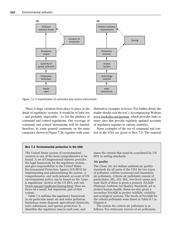
210 Environmental pollution
There is huge variation from place to place in thedetail of regulatory systems. It would be of little use– and probably impossible – to list the plethora ofcommand and control regulations. Our coverage ofcommand and control instruments will be limited,therefore, to some general comments on the maincategories shown in Figure 7.2b, together with some
illustrative examples in boxes. For further detail, thereader should visit the text’s Accompanying Websitewww.booksites.net/perman, which provides links tomany sites that provide regularly updated accountsof regulatory regimes in various countries.
Some examples of the use of command and con-trol in the USA are given in Box 7.2. The material
Figure 7.2 A classification of command and control instruments
Box 7.2 Environmental protection in the USA
The United States system of environmentalcontrols is one of the most comprehensive to befound. A set of Congressional statutes providesthe legal framework for the regulatory system,and give responsibility to the United StatesEnvironmental Protection Agency (US EPA) forimplementing and administering the system. Acomprehensive, and well-indexed, account of USenvironmental policy can be found on the ‘Laws& regulations’ section of the US EPA web site(www.epa.gov/epahome/lawreg.htm). Here wefocus on a small, but important, part of thatsystem.
Table 7.3 outlines the regulatory framework in six particular areas: air and water pollution,hazardous waste disposal, agricultural chemicals,toxic substances, and species protection. Itidentifies the regulatory area in each case, and
states the criteria that must be considered by USEPA in setting standards.
Air quality
The Clean Air Act defines ambient air qualitystandards for all parts of the USA for two typesof pollutant: criteria (common) and hazardous air pollutants. Criteria air pollutants consist ofparticulates, SO2, CO, NO2, low-level ozone andlead. Each of these is given a primary NAAQS(National Ambient Air Quality Standard), set toprotect human health. Some are also given asecondary NAAQS to protect wildlife, visibilityand ecological systems. The levels of NAAQS forthe criteria pollutants were listed in Table 6.7 inChapter 6.
The system for criteria air pollutants is asfollows. For stationary sources of air pollutants,
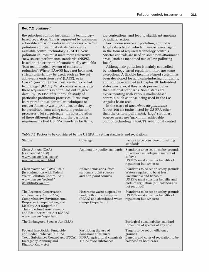
Pollution control: instruments 211
Table 7.3 Factors to be considered by the US EPA in setting standards and regulations
Statute
Clean Air Act (CAA) (as amended 1990)www.epa.gov/oar/oaqps/peg_caa/pegcaain.html
Clean Water Act (CWA) 1987(in conjunction with Federal Water Pollution Control Act)www.epa.gov/region5/defs/html/cwa.htm
The Resource Conservation and Recovery Act (RCRA)Comprehensive Environmental Response, Compensation, and Liability Act (Superfund)The Superfund Amendments and Reauthorization Act (SARA)www.epa.gov/superfund
The Endangered Species Act (ESA)
Federal Insecticide, Fungicide and Rodenticide Act (FIFRA)Toxic Substances Control Act (TSCA)Emergency Planning and Right-to-Know Act
Coverage
Ambient air quality standards
Effluent emissions, fromstationary point sources and non-point sources
Hazardous waste disposal onland, both current disposal(RCRA) and abandoned wastedumps (Superfund)
Restricting the use ofdangerous substancesFIFRA: agricultural chemicalsTSCA: toxic substances
Factors to be considered in settingstandards
Standards to be set on safety grounds(to achieve an ‘adequate margin ofsafety’)US EPA must consider benefits ofregulation but not costs
Standards to be set on safety groundsWaters required to be at least‘swimmable and fishable’US EPA must consider benefits andcosts of regulation (but balancing isnot required)
Standards to be set on safety groundsUS EPA must consider benefits ofregulation but not costs
Ecological sustainability standardProtection of species at any cost
Targets to be set on efficiencygroundsBenefits and costs of regulation to bebalanced in both cases
Box 7.2 continued
the principal control instrument is technology-based regulation. This is supported by maximumallowable emissions rates in some cases. Existingpollution sources must satisfy ‘reasonablyavailable control technology’ (RACT). Newpollution sources must meet more restrictive‘new source performance standards’ (NSPS),based on the criterion of commercially available‘best technological system of emissionsreduction’. Where NAAQS have not been met,stricter criteria may be used, such as ‘lowestachievable emissions rate’ (LAER), or in Class 1 (unspoilt) areas ‘best available controltechnology’ (BACT). What counts as satisfyingthese requirements is often laid out in greatdetail by US EPA after thorough study ofparticular production processes. Firms may be required to use particular techniques torecover fumes or waste products, or they may be prohibited from using certain productionprocesses. Not surprisingly, the interpretation of these different criteria and the particularrequirements that US EPA mandates for firms,
are contentious, and lead to significant amountsof judicial action.
For mobile source air pollution, control islargely directed at vehicle manufacturers, againin the form of required technology controls.Stricter controls are used in some non-attainmentareas (such as mandated use of low-pollutingfuels).
Although air pollution is mainly controlled by technology-based regulation, there are someexceptions. A flexible incentive-based system hasbeen developed for acid-rain-inducing pollutants,and will be examined in Chapter 10. Individualstates may also, if they wish pursue higher than national standards. Some states areexperimenting with various market-basedcontrols, such as those being used in the LosAngeles basin area.
In the cases of hazardous air pollutants(about 200 air toxins listed by US EPA other than the criteria pollutants), ‘large’ stationarysources must use ‘maximum achievable control technology’ (MACT). Additional control

212 Environmental pollution
measures, and/or new listed pollutants, may beadded by the US EPA if risk analysis suggeststhat this is warranted. With the passage of time,US EPA has gone some way along the process ofdefining acceptable risk in operational terms. Forexample, ‘ample margin of safety’ is now definedto mean that cancer risks to the most exposedpopulation do not exceed 1 in 10 000. (The long-term target has been specified as 1 in 1 millionfor the population at large.)7 Note from Table 7.3that the Clean Air Act requires the US EPA toonly take account of the benefits of control insetting regulations over toxic air emissions.However, in 1987 a Court of Appeals rulingfound that US EPA has been (unlawfully)considering both benefits and costs in settingambient standards. As a result, US EPA tightenedits standards (so that control was extended tocover emissions for which it previously felt thatthe cost-to-benefit ratio was too high to justifycontrol).
Clean water
Water standards are again typically based on technology controls. In the initial controlphase, this required the use of ‘best practicaltechnology’ (BPT). Later control phasesmandated the more stringent ‘best availabletechnology’ (BAT). In addition to BAT,dischargers must acquire (non-marketable)effluent emissions licences, often containing verydetailed plans about how discharges are treatedas well as the amounts that may be discharged.What counts as ‘best’ is defined by US EPA(although, again, not without much judicialchallenge). Technology controls (‘best-management practices’ are also employed to reduce runoff from non-point sources(industrial and agricultural sites).
Hazardous waste disposal
Under the terms of the Resource Conservationand Recovery Act, the US EPA has developed alist of about 450 hazardous substances. Disposalis controlled through location restrictions,required staff training, groundwater monitoringby disposing firms, and the requirement toconstruct detailed plans for site closure and post-
closure practice. Operators must also undertakesufficient insurance cover. These, and other,restrictions are supported by a licence system.An interesting innovation here is the adoption ofa ‘cradle-to-grave’ tracking and liability principle(see Box 7.1). The Superfund has provided amechanism for dealing with abandoned wastedumps. The fund is built up from generaltaxation and from taxes on the petroleum andchemical industries. The principle of ‘strict, jointand several liability’ (see Box 7.1) establishesstrong incentives throughout the waste cycle tominimise the amount of waste produced.
Toxic substances
The TSCA requires US EPA to review all newchemicals, and gives it authority to restrict useof, or ban, existing chemicals. Unlike most areasof environmental regulation, the TSCA requiresbalancing of the costs of regulation (in moneyterms) and the benefits of regulation (in terms ofcancer or other serious health impacts avoided).A study by Van Houtven and Cropper (1996)investigated US EPA bans on the use of asbestosin particular uses under the provisions of theTSCA. Of the 39 uses of asbestos it investigated,Van Houtven and Cropper found that US EPAwas able to measure costs and benefits in 31cases. Of these, 21 products were banned.
Agricultural chemicals
FIFRA imposes a duty of registration of all new pesticides. New ingredients in agriculturalchemicals cannot be introduced until the USEPA is satisfied, after cost–benefit analysis, thatthe product will generate positive net benefits.As an input to this study, manufacturers mustsubmit a detailed scientific study of theingredient. US EPA may also carry out SpecialReviews on existing pesticides. As with TSCA,FIFRA requires that the EPA ‘balance’ benefitsagainst costs in arriving at its decisions aboutbans or other restrictions. The Van Houtven and Cropper study investigated 245 food cropapplications of 19 pesticide active ingredients. Of these, 96 applications were banned after USEPA Special Reviews.
7 Actual risks have often been very much higher. A US EPA study in the late 1980s revealed that risks were worsethan 1 in 1000 in 205 communities around the country.
Box 7.2 continued

Pollution control: instruments 213
there shows that the administration of instruments isnot entirely separate from the setting of targets (or‘standards’ as they are also known). In the examples,the ‘goal’ passed on to the US Environmental Pro-tection Agency (USEPA) is given in the form of ageneral principle regarding the criterion that shouldbe used in setting standards, together with somedirection about what information should be used inits deliberations. The USEPA is then required totranslate that goal into specific targets and/or regula-tions and to administer their implementation.
In the sections that follow, we describe in a littlemore detail the three most commonly used types ofcommand and control instrument, and then invest-igate instruments that use the price mechanism tocreate incentives for pollution abatement. In doingso, the likely cost-efficiency of each instrument willbe discussed. A more complete appraisal of the rel-ative merits of each instrument using the criterialisted in Table 7.1 will be left until Section 7.6.
7.3.2.1 Non-transferable emissions licences
Suppose that the EPA is committed to attainingsome overall emissions target for a particular kind of pollutant. It then creates licences (also called permits or quotas) for that total allowable quantity.After adopting some criterion for apportioninglicences among the individual sources, the EPA dis-tributes licences to emissions sources. We use theterm non-transferable licences to refer to a systemwhere the licences cannot be transferred (exchanged)between firms: each firm’s initial allocation of pol-lution licences sets the maximum amount of emis-sions that it is allowed.8 Successful operation oflicence schemes is unlikely if polluters believe theiractions are not observed, or if the penalties on pol-luters not meeting licence restrictions are low relativeto the cost of abatement. Licence schemes will haveto be supported, therefore, by pollution monitoringsystems and by sufficiently harsh penalties for non-compliance.
Under special conditions, the use of such emis-sions licences will achieve an overall target at least
cost (that is, be cost-efficient). But it is highlyunlikely that these conditions would be satisfied. Weknow (see the first part of Appendix 7.1) that cost-efficiency requires the marginal cost of emissionsabatement to be equal over all abaters. If the EPAknew each polluter’s abatement cost function, it couldcalculate which level of emissions of each firm (andso which number of licences for each firm) wouldgenerate this equality and meet the overall target.
It is very unlikely that the EPA would possess, orcould acquire, sufficient information to set standardsfor each polluter in this way. The costs of collectingthat information could be prohibitive, and may out-weigh the potential efficiency gains arising fromintervention. Moreover, there is a problem of infor-mation asymmetries; those who possess the neces-sary information about abatement costs at the firmlevel (the polluters) do not have incentives to pro-vide it in unbiased form to those who do not have it(the regulator).9 We examine these incentives in alittle more detail in Section 7.6. A system of long-term relationships between regulator and regulatedmay overcome these asymmetries to some extent,but might bring other problems (such as high admin-istrative cost and regulatory capture – to be definedand explained in Chapter 8) in its wake. Given allthis, it seems likely that arbitrary methods will beused to allocate licences, and so the controls will notbe cost-efficient. Box 7.10 gives some indication ofhow great this cost-inefficiency is in practice.
7.3.2.2 Instruments which impose minimumtechnology requirements
Another command and control approach involvesspecifying required characteristics of productionprocesses or capital equipment used. In other words,minimum technology requirements are imposedupon potential polluters. Examples of this approachhave been variously known as best practicablemeans (BPM), best available technology (BAT) andbest available technology not entailing excessivecost (BATNEEC). Some further information ontechnology controls is given in Box 7.3.
8 We use the term ‘licence’ to denote non-transferable emissionsquotas. Later in the chapter, transferable quotas will be discussed.To avoid confusion, we call these ‘permits’.
9 Another possibility is that firms themselves may also beunaware of their abatement costs.

214 Environmental pollution
Box 7.3 Required technology controls
Regulations mandating the use of particulartechnologies are common forms of pollutioncontrol instrument in Europe, North America andthe other OECD countries. In the UK, a criterionunderlying required technology standards hasbeen ‘best practicable means’. The adjectivepracticable has never been given a precise legaldefinition, but the 1956 Clean Air Act stated that
Practicable means reasonably practicable havingregard, amongst other things, to local conditionsand circumstances, to the financial implicationsand the current state of technology.
Despite an element of tautology in this statement, it can be interpreted as meaning that a practicable control technology should betechnologically effective, subject to the constraintthat it is not excessively costly. In recent years,the cost qualification has been given greaterpriority, and has been enshrined in the principleof BATNEEC: the best available technology notentailing excessive cost. This puts the instrumentcloser to the kind advocated by economists, asthe ‘excessive cost’ condition implies a quasi-cost–benefit calculation in the administration of the instrument.
However, while the cost of control is oftenmeasured by the regulator in money terms (for
example, the additional money cost of one technique over another), the benefits are not usually measured in money terms; instead, benefits are seen in terms of reducedprobabilities of death or serious damage tohealth. In this sense, although some balancing ofcosts against benefits does often take place, theapproach being used is not ‘cost–benefit analysis’in the economics sense of that term. Rather thanusing the public’s estimate of benefits (in termsof willingness to pay) the regulator has to cometo a view as to what cost is reasonable to save alife or reduce a health risk. Some information on this is provided in Box 7.3a. Equivalent kinds of money-cost relative to health-benefitcomparisons are also made in the US regulatorysystem.
The manner in which technology-basedinstruments have been implemented variesconsiderably between countries. In the UK,officials of the Inspectorate of Pollution negotiatecontrols with plant managers, but have the right,in the last instance, to require the adoption ofcertain control technologies. The United StatesEnvironmental Protection Agency administers a rather more uniform control programme: in 1990, Congress required the EPA to establishtechnology-based standards for about 200specific pollutants.
Box 7.3a The value of life, as revealed by actions of the United States Environmental Protection Agency
A series of recent papers have attempted to deduce what value the United StatesEnvironmental Protection Agency (US EPA)places on saving lives. In one of these papers,Van Houtven and Cropper (1996) examined fourparticular areas over which the US EPA hassought to achieve regulation. We noted in Box7.2 that the US EPA can issue bans on particularuses of asbestos. Van Houtven and Cropperinvestigated 39 applications for asbestos use.From data on the costs of regulation and thenumber of lives expected to be saved in eachapplication, the authors were able to estimate thevalue of a statistical life that is implied by USEPA decisions. By definition, if an action resultsin the expected level of deaths falling by oneperson over some relevant time period, that
action has saved one statistical life. Van Houtvenand Cropper found that, on average, productswere banned when the cost of saving one lifewas below $49 million (in 1989 US dollarprices).
Van Houtven and Cropper obtain a verysimilar implied value ($51.51) million for a fatalcancer avoided in their study of 245 pesticideapplications (of which 96 were banned).Decisions here were taken under the auspices ofFIFRA agricultural chemicals legislation, whichalso requires cost and benefit balancing to beused by the US EPA. Van Houtven and Cropperalso investigated controls of toxic air pollutants – specifically benzene, arsenic, asbestos andmercury – under the provisions of the Clean AirAct. Prior to 1987, the implied value of a fatal
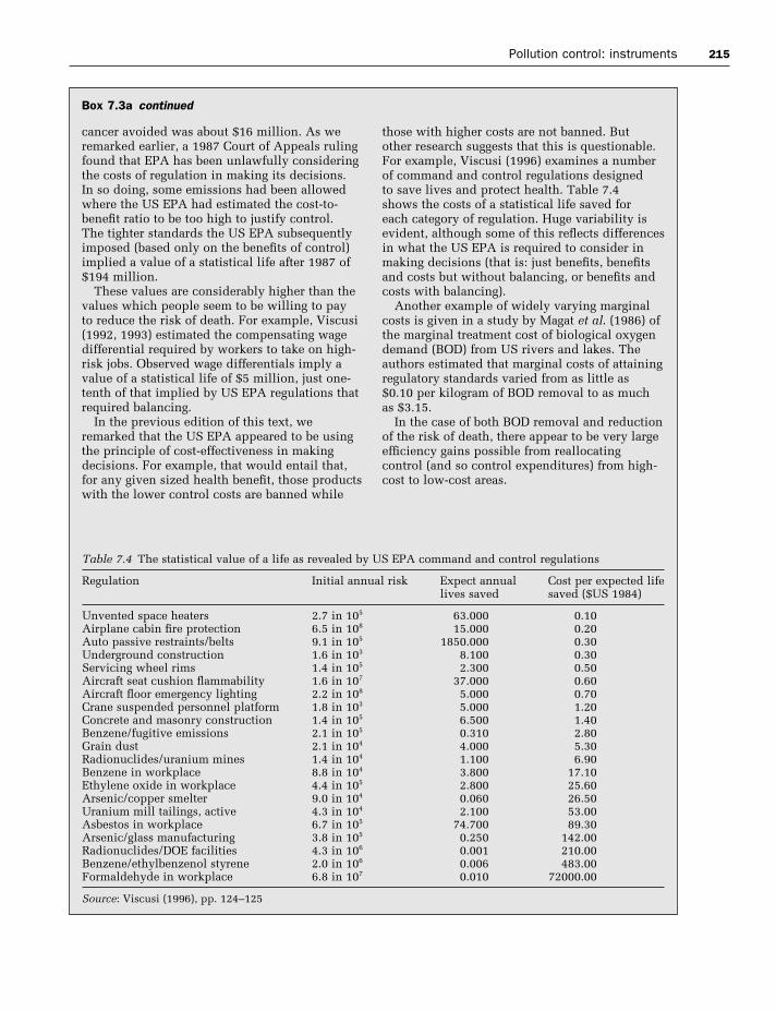
Pollution control: instruments 215
cancer avoided was about $16 million. As weremarked earlier, a 1987 Court of Appeals rulingfound that EPA has been unlawfully consideringthe costs of regulation in making its decisions. In so doing, some emissions had been allowedwhere the US EPA had estimated the cost-to-benefit ratio to be too high to justify control. The tighter standards the US EPA subsequentlyimposed (based only on the benefits of control)implied a value of a statistical life after 1987 of$194 million.
These values are considerably higher than thevalues which people seem to be willing to pay to reduce the risk of death. For example, Viscusi(1992, 1993) estimated the compensating wagedifferential required by workers to take on high-risk jobs. Observed wage differentials imply avalue of a statistical life of $5 million, just one-tenth of that implied by US EPA regulations thatrequired balancing.
In the previous edition of this text, weremarked that the US EPA appeared to be usingthe principle of cost-effectiveness in makingdecisions. For example, that would entail that,for any given sized health benefit, those productswith the lower control costs are banned while
those with higher costs are not banned. But other research suggests that this is questionable.For example, Viscusi (1996) examines a numberof command and control regulations designed to save lives and protect health. Table 7.4 shows the costs of a statistical life saved for each category of regulation. Huge variability isevident, although some of this reflects differencesin what the US EPA is required to consider inmaking decisions (that is: just benefits, benefitsand costs but without balancing, or benefits andcosts with balancing).
Another example of widely varying marginalcosts is given in a study by Magat et al. (1986) ofthe marginal treatment cost of biological oxygendemand (BOD) from US rivers and lakes. Theauthors estimated that marginal costs of attainingregulatory standards varied from as little as $0.10 per kilogram of BOD removal to as muchas $3.15.
In the case of both BOD removal and reductionof the risk of death, there appear to be very largeefficiency gains possible from reallocatingcontrol (and so control expenditures) from high-cost to low-cost areas.
Table 7.4 The statistical value of a life as revealed by US EPA command and control regulations
Regulation Initial annual risk Expect annual Cost per expected lifelives saved saved ($US 1984)
Unvented space heaters 2.7 in 105 63.000 0.10Airplane cabin fire protection 6.5 in 108 15.000 0.20Auto passive restraints/belts 9.1 in 105 1850.000 0.30Underground construction 1.6 in 103 8.100 0.30Servicing wheel rims 1.4 in 105 2.300 0.50Aircraft seat cushion flammability 1.6 in 107 37.000 0.60Aircraft floor emergency lighting 2.2 in 108 5.000 0.70Crane suspended personnel platform 1.8 in 103 5.000 1.20Concrete and masonry construction 1.4 in 105 6.500 1.40Benzene/fugitive emissions 2.1 in 105 0.310 2.80Grain dust 2.1 in 104 4.000 5.30Radionuclides/uranium mines 1.4 in 104 1.100 6.90Benzene in workplace 8.8 in 104 3.800 17.10Ethylene oxide in workplace 4.4 in 105 2.800 25.60Arsenic/copper smelter 9.0 in 104 0.060 26.50Uranium mill tailings, active 4.3 in 104 2.100 53.00Asbestos in workplace 6.7 in 105 74.700 89.30Arsenic/glass manufacturing 3.8 in 105 0.250 142.00Radionuclides/DOE facilities 4.3 in 106 0.001 210.00Benzene/ethylbenzenol styrene 2.0 in 106 0.006 483.00Formaldehyde in workplace 6.8 in 107 0.010 72000.00
Source: Viscusi (1996), pp. 124–125
Box 7.3a continued

216 Environmental pollution
In some variants of this approach, specific tech-niques are mandated, such as requirements to useflue-gas desulphurisation equipment in power gen-eration, designation of minimum stack heights, theinstallation of catalytic converters in vehicle exhaustsystems, and maximum permitted lead content inengine fuels. In other variants, production mustemploy the (technically) best technique available(sometimes subject to a reasonable cost qualifica-tion). The specific technique adopted is sometimesnegotiated between the EPA and the regulated par-ties on an individual basis.
Much the same comments about cost-effectivenesscan be made for technology controls as for licences.They are usually not cost-efficient, because theinstrument does not intrinsically focus abatementeffort on polluters that can abate at least cost. More-over, there is an additional inefficiency here that also involves information asymmetries, and whichrelates back to a point made earlier about Figure 7.2.Technology requirements restrict the choice setallowed to firms to reduce emissions. Decisionsabout emissions reduction are effectively being cent-ralised (to the EPA) when they may be better left tothe firms (who will choose this method of reducingemissions rather than any other only if it is least-costfor them to do so).
Required technology controls blur the pollutiontarget/pollution instrument distinction we have beendrawing in this and the previous chapter. The targetactually achieved tends to emerge jointly with theadministration of the instrument. We need to be a little careful here. Sometimes government sets ageneral target (such as the reduction of particulatesfrom diesel engines by 25% over the next 5 years)and then pursues that target using a variety of instru-ments applied at varying rates of intensity over time.In this case, no single instrument need necessarilyhave a particular target quantity associated with it.Nevertheless, it does matter (as far as cost-efficiencyis concerned) if the actual operation of any particularcomponent of this programme does not involve anycomparison of the benefits and costs of that com-ponent (because then the wrong mix of componentswill be used). There are many examples of techno-logy control where it appears to be the case thatemphasis is given almost exclusively to the costs ofpollution reduction technologies, and in particular to
what kind of cost premium is involved in using thetechnically best method as compared with its lower-ranked alternatives. (See Box 7.10, for example.And think about saving lives via safety regulations.)
Although technology-based instruments may belacking in cost-effectiveness terms, they can be verypowerful; they are sometimes capable of achievinglarge reductions in emissions quickly, particularlywhen technological ‘fixes’ are available but not widelyadopted. Technology controls have almost certainlyresulted in huge reductions in pollution levels com-pared with what would be expected in their absence.
7.3.2.3 Location
Pollution control objectives, in so far as they areconcerned only with reducing human exposure topollutants, could be met by moving affected per-sons to areas away from pollution sources. This isonly relevant where the pollutant is not uniformlymixing, so that its effects are spatially differentiated.Implementing this ex ante, by zoning or planningdecision, is relatively common. Ex post relocationdecisions are rarer because of their draconian nature.There have been examples of people being removedfrom heavily contaminated areas, including move-ments away from irradiated sites such as Chernobyl,Times Beach (Missouri) and Love Canal (NewYork). However, it has been far more common tomove pollution sources away from areas where people will be affected, or to use planning regula-tions to ensure separation. Planning controls andother forms of direct regulation directed at locationhave a large role to play in the control of pollutionwith localised impacts and for mobile source pollu-tion. They are also used to prevent harmful spatialclustering of emission sources.
Location decisions of this kind will not be appro-priate in many circumstances. Moving people awayfrom a pollution source cannot, for example, reduceimpacts on ecosystems. Relocating (or planning thelocation of new) emission sources has wider applicab-ility, but will be of no use in cases where pollutionis uniformly mixing. In Section 7.5 we shall con-sider a number of incentive-based instruments that aredesigned, among other things, to influence the spatiallocation of emissions sources. These are not, how-ever, examples of command and control instruments.
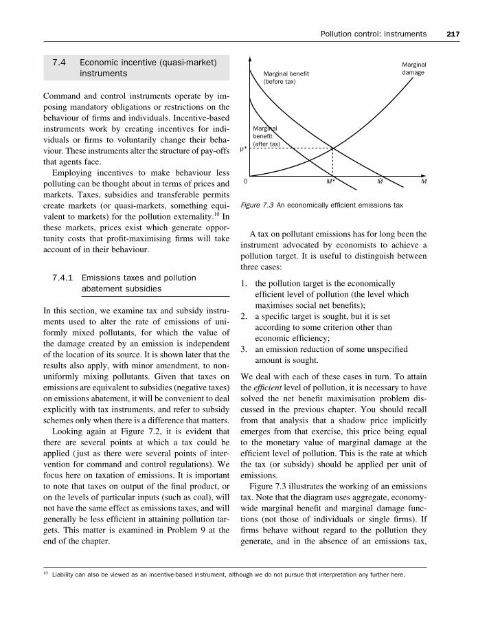
Pollution control: instruments 217
7.4 Economic incentive (quasi-market) instruments
Command and control instruments operate by im-posing mandatory obligations or restrictions on thebehaviour of firms and individuals. Incentive-basedinstruments work by creating incentives for indi-viduals or firms to voluntarily change their beha-viour. These instruments alter the structure of pay-offsthat agents face.
Employing incentives to make behaviour less polluting can be thought about in terms of prices andmarkets. Taxes, subsidies and transferable permitscreate markets (or quasi-markets, something equi-valent to markets) for the pollution externality.10 Inthese markets, prices exist which generate oppor-tunity costs that profit-maximising firms will takeaccount of in their behaviour.
7.4.1 Emissions taxes and pollutionabatement subsidies
In this section, we examine tax and subsidy instru-ments used to alter the rate of emissions of uni-formly mixed pollutants, for which the value of the damage created by an emission is independent of the location of its source. It is shown later that theresults also apply, with minor amendment, to non-uniformly mixing pollutants. Given that taxes onemissions are equivalent to subsidies (negative taxes)on emissions abatement, it will be convenient to dealexplicitly with tax instruments, and refer to subsidyschemes only when there is a difference that matters.
Looking again at Figure 7.2, it is evident thatthere are several points at which a tax could beapplied ( just as there were several points of inter-vention for command and control regulations). Wefocus here on taxation of emissions. It is importantto note that taxes on output of the final product, oron the levels of particular inputs (such as coal), willnot have the same effect as emissions taxes, and willgenerally be less efficient in attaining pollution tar-gets. This matter is examined in Problem 9 at theend of the chapter.
A tax on pollutant emissions has for long been theinstrument advocated by economists to achieve apollution target. It is useful to distinguish betweenthree cases:
1. the pollution target is the economicallyefficient level of pollution (the level whichmaximises social net benefits);
2. a specific target is sought, but it is setaccording to some criterion other thaneconomic efficiency;
3. an emission reduction of some unspecifiedamount is sought.
We deal with each of these cases in turn. To attainthe efficient level of pollution, it is necessary to havesolved the net benefit maximisation problem dis-cussed in the previous chapter. You should recallfrom that analysis that a shadow price implicitlyemerges from that exercise, this price being equal to the monetary value of marginal damage at theefficient level of pollution. This is the rate at whichthe tax (or subsidy) should be applied per unit ofemissions.
Figure 7.3 illustrates the working of an emissionstax. Note that the diagram uses aggregate, economy-wide marginal benefit and marginal damage func-tions (not those of individuals or single firms). Iffirms behave without regard to the pollution theygenerate, and in the absence of an emissions tax,
10 Liability can also be viewed as an incentive-based instrument, although we do not pursue that interpretation any further here.
Figure 7.3 An economically efficient emissions tax

218 Environmental pollution
emissions will be produced to the point where theprivate marginal benefit of emissions is zero. This isshown as !, the pre-tax level of emissions.
Now suppose an emissions tax was introduced atthe constant rate µ* per unit emission, the value ofmarginal damage at the efficient pollution level.Given this, the post-tax marginal benefit schedulediffers from its pre-tax counterpart by that value ofmarginal damage. Once the tax is operative, profit-maximising behaviour by firms leads to a pollutionchoice of M* (where the post-tax marginal benefitsof additional pollution are zero) rather than ! as wasthe case before the tax. Note that levying an emis-sions tax at the rate µ* creates just the right amountof incentive to bring about the targeted efficientemission level, M*.11
It is sometimes more convenient to view the prob-lem in terms of abatement, Z, rather than the level ofpollution itself. This can be done by reinterpretingFigure 7.3. Viewed in this new light, the emissiontax causes abatement to increase from zero (at !) to its efficient level Z* = ! − M* at the point M* onthe horizontal axis. Alternatively, we can map therelevant parts of Figure 7.3 into abatement space,from which we obtain Figure 7.4. It is important tobe clear about the relationships between these two diagrams. First, the curve labelled ‘marginal cost ofabatement’ is just the mirror image of the (before-tax) marginal benefit curve in Figure 7.3; what firms
privately forgo when they abate emissions is, ofcourse, identical to the benefits they receive fromemissions. The ‘marginal benefit of abatement’ to arepresentative firm is the tax rate applied, µ*. Eachunit of abated emissions reduces the firm’s total taxbill by that amount. As the tax rate is constant, themarginal benefit of abatement curve is horizontal.Secondly, note that we have truncated the twocurves in Figure 7.4 at Z = W, where W is identical inmagnitude to !. Confirm for yourself the reason fordoing this. Finally, note that Z* = ! − M*, and sothe distance from the origin to Z* in Figure 7.4 isequal to the horizontal distance between ! and M*along the emissions axis in Figure 7.3.
In the absence of an emissions tax (or an abate-ment subsidy), firms have no economic incentive toabate pollution. (In terms of Figure 7.4, the marginalbenefit of abatement lies at zero along the Z axis.)Profit-maximising behaviour implies that firmswould then undertake zero abatement, correspond-ing to emissions !. However, when an emissionstax is levied (or, equivalently, when an abatementsubsidy is available) an incentive to abate exists inthe form of tax avoided (or subsidy gained). It willbe profitable for firms to reduce pollution as long as their marginal abatement costs are less than thevalue of the tax rate per unit of pollution (or lessthan the subsidy per unit of emission abated). If the tax/subsidy is levied at the level µ* the efficientpollution level is attained without coercion, purelyas a result of the altered structure of incentives facing firms.
In the language of externalities theory, the taxeliminates the wedge (created by pollution damage)between private and socially efficient prices; the taxbrings private prices of emissions (zero) into linewith social prices (µ*). The tax ‘internalises theexternality’ by inducing the pollution generator tobehave as if pollution costs entered its private costfunctions. Decisions will then reflect all relevantcosts, rather than just the producer’s private costs,and so the profit-maximising pollution level willcoincide with the socially efficient level. Not onlywill the tax instrument (at rate µ*) bring about anefficient level of pollution but it will also achieve
Figure 7.4 The economically efficient level of emissionsabatement
11 As shown in Appendix 7.1, a subsidy at the rate µ* on units of pollution abated would have an equal short-run effect on emissions toa pollution tax at the rate µ* on unabated units of pollution.

Pollution control: instruments 219
that target in a cost-effective way. Remember thatcost-efficiency requires that the marginal abatementcost be equal over all abaters. Under the tax regimeall firms adjust their firm-specific abatement levelsto equate their marginal abatement cost with the tax rate. But as the tax rate is identical for all firms,so are their marginal costs.
Our discussion in this section so far has dealt withthe case in which the EPA wishes to attain the eco-nomically efficient level of emissions, M*. How-ever, we saw in the previous chapter that the EPAmay not have sufficient information for this to befeasible. Suppose that the EPA does have an emis-sions target, %, set perhaps on health grounds. Toattain this (or indeed any other specific) emissionstarget, knowledge of the aggregate (economy-wide)marginal emissions abatement cost function wouldbe sufficient. This should be clear by looking atFigure 7.4 again. For any target %, knowledge of the aggregate marginal cost of abatement functionallows the EPA to identify the tax rate, say 7, thatwould create the right incentive to bring about thatoutcome. Even though the target is not an efficienttarget, the argument used above about cost-efficiencyremains true here: the emissions tax, levied at 7,attains the target % at least total cost, and so is cost-efficient. This result is rather powerful. Not onlydoes the EPA not need to know the aggregatemarginal pollution damage function, it does not needto know the abatement cost function of each firm.Knowledge of the aggregate abatement cost functionalone is sufficient for achieving any arbitrary targetat least cost. Compare this result with the case ofcommand and control instruments; there, knowledgeof every firm’s marginal abatement cost function isrequired – a much more demanding informationrequirement.
Finally, let us deal with the third of the listedcases where an emission reduction of some unspe-cified amount is sought. Without knowledge of any-thing about abatement costs and benefits, the EPAcould select some arbitrary level of emissions tax,say 8. Faced with this tax rate, profit-maximisingfirms will reduce emissions up to the point wheremarginal abatement costs are brought into equalitywith this tax rate. As all firms do this the emissionsreduction is achieved at least cost, once again.Although the government cannot know in advance
how much pollution reduction will take place, it can be confident that whatever level of abatement is generated would be attained at minimum feasiblecost. Taxes (and subsidies by an equivalent argu-ment) are, therefore, cost-efficient policy instru-ments. These results are demonstrated formally inAppendix 7.1, Parts 4 and 5.
We stated earlier that an emissions tax and anemissions abatement subsidy (at the same rate) havean identical effect in terms of pollution outcome inthe short term (see Part 6 of Appendix 7.1). How-ever, the two instruments do have some very import-ant differences. Most importantly, the distribution ofgains and losses will differ. Taxes involve net trans-fers of income from polluters to government, whilesubsidies lead to net transfers in the other direction(see Problem 4). This has important implications forthe political acceptability and the political feasibilityof the instruments. It also could affect the long-runlevel of pollution abatement under some circum-stances. Some more discussion on this matter isgiven in Box 7.4.
To reinforce your understanding of this materialin this section, you are recommended to workthrough Problem 10 at the end of this chapter. Thisuses an Excel workbook to simulate emissionsreduction using command and control techniques,tax and subsidy instruments, and (to be discussed inthe next section) transferable permits. Some infor-mation on practical experience with pollution taxesand abatement subsidies is given in Box 7.5.
7.4.2 Marketable emissions permits
As with command and control and tax/subsidyinstruments, marketable permits (also known astradable or transferable permits) can be applied atmany points in the production-to-pollution processrepresented in Figure 7.2. Here we consider only oneform: permits on the quantity of emissions. Market-able permit systems are based on the principle thanany increase in emissions must be offset by anequivalent decrease elsewhere. There is a limit seton the total quantity of emissions allowed, but theregulator does not attempt to determine how thattotal allowed quantity is allocated among individualsources.

220 Environmental pollution
Box 7.4 Are pollution taxes and emissions abatement subsidies equivalent?
For an industry of a given size, an emission taxand an abatement subsidy levied or paid at thesame rate are equivalent in terms of units ofemissions abated. Thus, looking at Figure 7.3again, a subsidy or a tax at the rate µ* wouldreduce emissions from H to M* for a single firmwith a given capital structure. As the industry is simply the sum of all firms, if the number offirms remains constant and the capital structureof each firm is unchanged, then the effects oftaxes and subsidies are identical.
However, the two instruments are different intheir effects on income distribution. A firm gainsadditional income from an abatement subsidy, as it will undertake abatement only when theunit abatement subsidy exceeds its marginalabatement cost. A tax on the other hand resultsin a loss of income to the firm as it pays the taxon all its emissions. To make this comparisonmore precise, look at Figure 7.5, the functions in which reproduce those in Figure 7.3.
An abatement subsidy will result in a paymentto the firm equal to the areas S1 + S2, that is, µ*multiplied by (H − M*). However, by reducingemissions from H to M* the firm loses S2 in profiton final output. The net gain to the firm is equal,therefore, to the area S1. A tax levied at the rateµ* on emissions M* will cost the firm µ*M*, that is, the sum of the areas S3, S4, S5 and S6.
However, by reducing emissions from H to M*the firm also loses profit on reduced output, thearea S2. So the income effects are entirelydifferent.
Let us explore this difference a little further.Recall that the tax paid is equal in value toµ*M*, while the subsidy received is µ*(H − M*).But µ*(H − M*) = µ*H − µ*M*. The second termon the right-hand side is the tax paid, and willdepend on the amount of abatement undertaken.It is this second component which gives the firman incentive to abate emissions. Recalling that µ is an outflow in a tax scheme and an inflow in a subsidy scheme, an outflow of µ*M* (with a tax) is identical to an inflow of −µ*M* (with asubsidy). The two incentive effects are identical,and it is this that forms the basis for the claimthat the instruments are equivalent. However, the subsidy differs from the tax by the presenceof the additional term, µ*H, a fixed or lump-sum payment, independent of the amount ofabatement the firm actually undertakes. In thelong run such payments may alter industryprofitability, and so alter the size of the industryitself. This lump-sum payment component of thesubsidy may destroy the equivalence between the two instruments in terms of their effects onemissions abatement.
We are faced with the possibility that asubsidy might enlarge the industry, partially or wholly offsetting the short-run emissionsreduction. It is not possible to be more preciseabout the final outcome, as that depends onseveral other factors, including whether or notgovernment introduces other fiscal changes tocounteract the income effects we have justdescribed. A general equilibrium analysis wouldbe necessary to obtain clear results. This isbeyond our scope in this text, so we just notethat the equivalence asserted above is not validin all cases.
Finally, note another aspect of an abatementsubsidy scheme. As one component of thesubsidy payment depends on the uncontrolledlevel of emissions (that is, the component µ*H),a firm has an incentive to misrepresent theuncontrolled level of emissions in order to obtaina favourable benchmark in terms of which thesubsidy payments are calculated.
Figure 7.5 Emissions tax and abatement subsidyschemes: a comparison

Pollution control: instruments 221
Box 7.5 The use of economic instruments in OECD countries
The use of economic instruments to achieveenvironmental goals has increased markedlysince the 1970s. The number of applications hasincreased, as has the variety of instruments used.Revenues from environmentally related taxes in2000 constituted about 7% of total OECD taxrevenue, a figure that is growing steadily andwhich had accelerated at the end of the 1990s.
User charges and subsidies were being appliedin the 1970s. Since then, emissions charges andtaxes have become widespread, subsidies toencourage the installation or use ofenvironmentally friendly capital equipment havebecome common, and several other incentive-based instruments have appeared for the firsttime, including deposit-refund systems andperformance bonds. The use of marketablepermits has began to appear, although it is as
yet not widely spread. Table 7.5 lists the maincategories of economic instruments and theirusage in OECD economies. Box 7.6 considersseveral examples of the use of emissions taxesand emissions abatement subsidies.
Economic instruments are also widely used for natural resource management. Commonapplications are in the management of waterquantity (typically abstraction charges or taxes),fisheries (taxes, fees and transferable quotas),forestry (charges and subsidies) and wetlands(financial assistance to owners). Economicinstruments are also used to preserve soil andland quality, and to preserve species and wildlife(typically fees and permits). Several examples of resource management or conservationinstruments are given in the resource harvestingchapters (17 and 18) later in the text.
Table 7.5 Economic instruments used in OECD countries
Country Fees, charges Tradable Deposit-refund Non-compliance Performance Liability Subsidiesand taxes permits systems fees bonds payments
Australia • • • • •Austria • • •Belgium •Canada • • • • • • •Czech Republic • • • •Denmark • • • • •Finland • • • •France • • •Germany • •Greece • • •Hungary • • •Iceland • •Ireland •Italy • •Japan • • •Korea • • •Mexico • •Netherlands • • •New Zealand •Norway • • • •Poland • • • • •Portugal •Spain •Sweden • • • • •Switzerland • • •Turkey • • • • •UK •USA • • • • • •
Source: OECD (1999)Notes to Table 7.5:1. Entries marked by • denote that the instrument category was stated to be used (or to have been used) by the country
in question in response to a questionnaire-based survey of all (29) OECD economies in 1999. 24 countries responded.Non-respondent countries are those for which there are no entries in this table in any column except that labelled ‘Fees, charges and taxes’
2. ‘Charges’ refer to requited emissions charges, user charges and product charges

222 Environmental pollution
Box 7.6 Emissions tax and abatement subsidies in practice12
The majority of emissions taxes in current useapply to the transport and energy sectors. A thirdimportant application is to waste management.Emissions fees were used in at least 20 OECDcountries in 1999, and their use has beengrowing steadily since 1985. The OECD now lists approximately 200 examples of fees or taxesin the areas of air, water and noise pollution, and waste disposal. In some cases, tax revenuesare earmarked for purposes of environmentalimprovement. In Germany and Italy, charges are used in conjunction with effluent standards:those firms which meet or better the standardsare taxed at a lower rate per unit effluent thanothers.
Air-pollutant emissions charges are being used predominantly in Japan and a number ofEuropean countries. France has used charges as an incentive to install pollution abatementtechnology, with charges being repaid in theform of capital subsidies to firms adoptingrecommended control technologies. In 1998,France integrated several existing charges into a unified ‘General Tax on Polluting Activities’(TGAP); the environmental agency is allocated a share of TGAP revenues for environmentalimprovement programmes. Sweden chargescombustion plants for NOX emissions, withrevenue being distributed among emitters inproportion to their share in total energy output.Hence the total cost of the system to emitters iszero, but each plant has an incentive to reduceits emissions-to-energy-output ratio. The regimeappears to have led to significant falls in NOX
emissions and to have spurred innovation incombustion technology. In Japan emissionslevies are earmarked as a compensation fund for victims of air pollution; charge levels aredependent upon amounts of compensation paid out in previous years.
Several countries – including Australia, the Czech Republic, Hungary and Iceland – have systems of charges for ozone-depletingsubstances. Differential tax rates on leaded and unleaded petrol in the United Kingdomserve as an indirect charge on lead emissions,and Sweden has used differential charges and subsidies on cars and heavy vehicles toencourage the purchase of low-pollution enginesand the adoption of catalytic converters. Thereare relatively high rates of tax on electricity and
primary energy sources throughout WesternEurope; while not being pollution taxes as such, they do have similar incentive effects byencouraging energy conservation and enhancingenergy efficiency.
Although the European Union has abandonedplans for a common carbon tax, Denmark,Finland, Italy, the Netherlands, Norway, Swedenand the UK all currently use some form of energytax which, to varying degrees, reflects the carboncontent of fuels. However, in the great majorityof countries where CO2 (or other environmental)taxes have been implemented, some sectors havebeen exempted from the tax, or the tax rate isdifferentiated across sectors. This reduces thecost-effectiveness, and so raises the real cost, ofthe tax.
Water effluent charges are used in Australia,Belgium, Canada, the Czech Republic, France,Italy, Germany, Mexico, the Netherlands, Poland and several US states. Charge rates varyaccording to the quantity and quality of wastewater. The UK has a landfill tax; this is examinedin Box 7.7.
The USA makes little use of emissions taxes or charges. Exceptions include a tax onchlorofluorocarbons to help in the phasing out of these chemicals, and fees on sewage and solidand hazardous waste at landfills. Householdstypically pay by the gallon for sewage disposal,and waste haulage firms pay by the ton for solidwaste disposal. However, household andbusiness enterprises have traditionally paidlump-sum charges for solid waste disposal, and so marginal disposal costs are not passed on to the initial producers of waste, leading tosignificant efficiency losses. As more states moveto volume-related charges (37 states now do this),volumes discarded have fallen and recyclingrates have risen significantly (Anderson et al.,1997). The United States has, though, made moreextensive use of marketable emission permitinstruments than have European economies (see Box 7.8).
Tax rates are typically set at levels insufficient to fully internalise external costs(EEA, 2000). Low rates of tax or subsidy implycorrespondingly low levels of impact. In somecases charges have been high enough to havelarge incentive effects. The Netherlands, with relatively high rates, has shown large
12 In this box we do not distinguish between taxes and fees or charges, using the terms interchangeably.
Pollution control: instruments 223
There are two broad types of marketable emissionpermit systems – the ‘cap-and-trade’ system and theemission reduction credit (ERC) system. We shallanalyse the cap-and-trade approach in some depth,and briefly consider the ERC system in Section7.4.2.4 below.
A cap-and-trade marketable emission permitsscheme for a uniformly mixing pollutant involves:13
n A decision as to the total quantity of emissionsthat is to be allowed (the ‘cap’). The totalamount of permits issued (measured in units ofpollution) should be equal to that target level ofemissions.
n A rule which states that no firm is allowed toemit pollution (of the designated type) beyondthe quantity of emission permits it possesses.
n A system whereby actual emissions aremonitored, and penalties – of sufficient deterrentpower – are applied to sources which emit inexcess of the quantity of permits they hold.
n A choice by the control authority over how the total quantity of emission permits is to beinitially allocated between potential polluters.
n A guarantee that emission permits can be freelytraded between firms at whichever price isagreed for that trade.
Box 7.7 Landfill tax example
A landfill tax was introduced in the UK in1996. The tax, paid by landfill operators, is set at different rates for inactive waste such as bricks (£2 per tonne) and other waste (£7 per tonne). An element of tax neutrality is imposed by reducing employers’ nationalinsurance contributions to offset the costs ofthe landfill tax.
The tax is designed so that incentives exist to reduce waste flows. However, since its inception, operation of the tax has beenplagued by concerns that waste has beendisposed of illegally to avoid landfill taxcharges. This illustrates the point thatincentive-based instruments for environmentalcontrol may be ineffective unless there iscareful monitoring and methods for ensuringcompliance.
Charges levied on landfill operators are alsofound in the Czech Republic (since 1992). Thetax is in two parts, the first being imposed onall landfill operators (with revenues recycledto municipal authorities for environmentalprotection activities). The second component – strictly speaking, a non-compliance fee –charges operators who fail to attain specifiedstandards. Evidence suggests that the tax hasmarkedly increased the proportion of sitesattaining specified standards. A similar systemoperates in the Slovak Republic. It is morecommon for charges to be placed on generatorsof waste (rather than disposers of it), withapplications in China, Estonia, Hungary,Poland and Russia.
improvements in water quality. Sweden’s use of differential taxes and subsidies, and thedifferential tax on unleaded petrol in the UKhave been very effective in causing substitutionin the intended directions. In some instances, therevenues from specific charges are earmarked forparticular forms of environmental defence orclean-up expenditure – one example is the use of taxes on new paint purchases in BritishColumbia to support reprocessing and safedisposal of used paint.
Subsidies for attainment of environmentalimprovements are used widely. A few countriesuse subsidies that are proportionately related to
quantities of air emissions or water effluent. It is far more common, though, for subsidies tobe paid in the form of grants, tax allowances orpreferential loans for capital projects that areexpected to lead to environmental improvements(such as low-emissions vehicles, cleaner waste-treatment plants or the development ofenvironmentally friendly products). Theseschemes are often financed from earmarkedenvironmental funds. A comprehensive listing of such schemes can be found on the web page of OECD (1999).
Sources: Tietenberg (1990), Goodstein (1995), OECD (1999)
Box 7.6 continued
13 We deal with marketable permits for non-uniformly-mixing pol-lutants in Section 7.5.3.
224 Environmental pollution
Marketable permit schemes differ from tax orsubsidy schemes by working in terms of quantitiesrather than prices. But this feature is also true forcommand and control instruments such as quotas,licences and standards. The distinguishing feature isthe transferability of permits between individualsources in the marketable permits case. Permit trad-ing is not allowed in command and control licencesystems.
It is the exchange process that generates theattractive qualities of the marketable permit system.In effect, tradability creates a market in the right topollute. In that market, the right to pollute will havea value, given by the prevailing market price. So thedecision to pollute generates an opportunity cost. Byemitting an extra unit of the pollutant, one unit ofpermit is used up and so cannot be sold to anotherfirm. The firm incurs a cost in emitting each unit of the pollutant, that cost being the current marketpermit price. Intuitively, this suggests that a market-able permit system should be equivalent (at least insome ways) to a tax or subsidy system, provided thepermit price is equal to the tax or subsidy rate. As weshall see, this intuition is correct.
Let us consider how an equilibrium price mightemerge in the market for permits. Suppose that permits have been allocated at no charge to firms insome arbitrary way. Once this initial allocation hastaken place, firms – both those holding permits insufficient number to cover their desired emissionlevels and those not holding sufficient for that pur-pose – will evaluate the marginal worth of permits tothemselves. These valuations will differ over firms.
Some firms hold more permits than the quantity of their desired emissions (in the absence of anycontrol). The value of a marginal permit to thesefirms is zero.14 Others hold permits in quantitiesinsufficient for the emissions that they would havechosen in the absence of the permit system. Themarginal valuations of permits to these firms willdepend upon their emission abatement costs. Somewill have high marginal abatement costs, and so arewilling to pay high prices to purchase emissionspermits. Others can abate cheaply, so that they are
willing to pay only small sums to purchase permits;their marginal permit valuation is low.
Indeed, it is not necessarily the case that a firmwhich holds fewer permits than its desired emissionslevel will buy permits. It always has the option avail-able to reduce its emissions to its permitted level byundertaking extra abatement. The firm may find itpreferable to sell permits (rather than buy them) ifthe price at which they could be sold exceeds itsmarginal abatement cost.
In any situation where many units of a homo-geneous product are held by individuals with sub-stantially differing marginal valuations, a market for that product will emerge. In this case, the product istradable permits, and the valuations differ becauseof marginal abatement cost differences betweenfirms. Therefore, a market will become establishedfor permits, and a single, equilibrium market pricewill emerge, say µ. Notice that trading does not alterthe quantity of permits in existence, it merely redis-tributes that fixed amount between firms.
In equilibrium marginal abatement costs will beequal over all firms. It is this property of the systemwhich ensures that transferable marketable permits,like taxes and subsidies, achieve any given target atleast cost. Moreover, another equivalence arises. Ifthe total quantity of permits issued is M* and thatquantity is identical to the level of emissions whichwould emerge from an emissions tax (or an abate-ment subsidy) at the rate µ* then a marketable per-mit scheme will generate an equilibrium permitprice µ*. In effect, the marketable permit system isan equivalent instrument to either emissions taxes oremissions abatement subsidies. We demonstrate thisresult algebraically in Part 7 of Appendix 7.1.
7.4.2.1 The initial allocation of permits
The implementation of a marketable permits systemrequires that the EPA select a method by which thetotal allowable quantity of permits (the cap) is ini-tially allocated among sources. Simplifying matterssomewhat, we can envisage that it must choose oneof the following:
14 If permits were storable or ‘bankable’ so that they could beused in the future, their worth would be positive (rather than zero)as there will be some positive probability that they could be used
later when the firm would otherwise have insufficient permits tocover desired emissions. But we shall leave this complication toone side for now.

Pollution control: instruments 225
n the EPA sells all permits by auction;n the EPA allocates all permits at no charge
(which in turn requires that a distribution rule bechosen).
We shall now investigate how the market price ofpermits is determined in each of these two cases.
7.4.2.2 Determination of the equilibrium marketprice of permits
Case 1: Auctioned permits
Suppose that the permits are initially allocatedthrough a competitive auction market. Individualfirms submit bids to the EPA. When ranked indescending order of bid price, the resulting schedulecan be interpreted as a market demand curve for permits. Assuming that no strategic behaviour takesplace in the bidding process, this demand curve willbe identical to the aggregate marginal abatementcost function.
The market equilibrium permit price is deter-mined by the value of the aggregate marginal abate-ment cost at the level of abatement implied by thetotal number of issued permits.15 This is illustratedin Figure 7.6. The demand curve for permits is theaggregate marginal abatement cost function for allpolluting firms. The total number of permits (allowedemissions) is M*. Given this quantity of permits, the
market price for permits will be µ*. Firms collect-ively are required to reduce emissions from ! toM*.
Case 2: Free initial allocation of permits on anarbitrary basis
Alternatively, the EPA may distribute the permits atno charge, and allow them to be subsequently tradedin a free market. The initial allocation is unlikely tocorrespond to the desired (that is, profit-maximising)holdings of permits (and in aggregate, of course, islikely to be less than total desired emissions). Somefirms will try to buy additional permits from others,while others will try to sell some of their initial hold-ing. Buyers will typically be firms with relativelyhigh marginal abatement costs, who hope to pur-chase additional quantities at a price less than theirmarginal abatement cost. Sellers will be those in anopposite position, hoping to sell some permits at aprice greater than their marginal abatement cost.
In a well-functioning competitive market, themarket price that would emerge in this case wouldbe identical to that which would be established ifpermits were sold at a competitive auction. This is portrayed in Figure 7.7. Note that the quantitytraded, EP*, is less than the number of permitsissued by the EPA (M*), because trades only takeplace as holdings are adjusted to desired levels.
15 It is assumed here that all permits are sold at one price (the highest single price consistent with selling all permits).
Figure 7.6 The determination of the market price ofemissions permits Figure 7.7 The determination of the market price of
emissions permits: free initial allocation case

226 Environmental pollution
It is clear that the method by which permits areinitially allocated has no bearing on the amount ofabatement that takes place; that depends only on thetotal number of permits issued. What is, perhaps,less evident is that the method of initial allocationalso has no effect on the equilibrium permit price.
There is one important qualification to theseremarks about permit price determination. We haveassumed that the market behaves as if it were per-fectly competitive. But if the polluting industry inquestion is dominated by a small number of firms, or if for any reason the quantity of trading is small,strategic behaviour may take place. This could happen both in permit auctions and where firms areadjusting permit holdings from their initial alloca-tions to their profit-maximising levels. Strategicbehaviour may cause the market price of permits todiverge from its competitive level.
A simple numerical illustration (which extends an example used earlier in the chapter) will help tostrengthen understanding about the way that thisinstrument operates. Consider the information shownin Table 7.6. We suppose that the EPA selects anemissions cap – and so a total permit allocation – of 50 units. The pollutant is emitted by just twofirms, A and B, and emissions abatement can only beundertaken by these firms. The EPA decides arbit-rarily to allocate half of total permits to each firm, so prior to trading A and B are each allowed to emit25 units of the pollutant. As in our earlier discussion,we assume that in the absence of any control systemA would choose to emit 40 units and B 50 units.
Given the initial permit allocations, A must reduceemissions by 15 units and B by 25 units. It can beseen from Figure 7.8 (which reproduces exactly theabatement cost functions used previously in Figure7.1) that A has a marginal abatement cost of 45 andB a marginal abatement cost of 125.
The fact that firm A has lower marginal abatementcost than firm B after the initial permit allocationimplies that the total abatement of 40 units of emis-sion is not being achieved at least cost. Moreover, B places a much higher value on an incremental per-mit than does A (125 as compared with 40). Thusthe two will find it mutually beneficial to trade withone another in permits. What will be the outcome ofthis trade? If the market behaved as if it were a com-petitive market, an equilibrium market price of 75would emerge. At that price, firm B (the high-costabater) would buy permits and A (the low-costabater) would sell permits. In fact, A would buy 10permits from A at 75 each, because for each of those
Table 7.6 Emissions abatement data for firms A and B
A B A + B
Uncontrolled emissions 40 50 90
Uncontrolled abatement 0 0 0
Efficient emissions 15 35 50
Efficient abatement 25 15 40
Initial permit allocation 25 25 50
Final permit allocation 15 35 50
Figure 7.8 Efficient abatement with two firms and marketable permits

Pollution control: instruments 227
10 permits, it would be paying less than it wouldcost the firm to abate the emissions instead. Con-versely, B would sell 10 permits to A at 75 each,because for each of those 10 permits, it would bereceiving more than it would cost the firm to abatethe emissions instead.
Trading finishes at the point where A has 15 per-mits (10 less than its initial allocation) and B has 35(10 more than its initial allocation). Marginal controlcosts are equalised across polluters, and the totalcost of abating emissions by 40 units has therebybeen minimised. The permit system will, therefore,have identical effects on output and emissions as anoptimal tax or subsidy system, and will be identicalin terms of its cost-effectiveness property.
One other feature shown in Figure 7.8 should be noted. The line labelled MC(Industry) is theindustry-wide (or aggregate) marginal cost of abatement schedule. It is obtained by summing horizontally the two firm’s marginal abatement costfunctions, and is given by16
The equilibrium permit price is found as the industry marginal cost (75) at the required level ofindustry abatement (40). Note that as the requiredabatement rises, so will the equilibrium permit price.
7.4.2.3 Marketable permit systems and thedistribution of income and wealth
In a perfectly functioning marketable permit sys-tem the method of initial allocation of permits has no effect on the short-run distribution of emissionsbetween firms. But it does have significant effects onthe distribution of income and wealth between firms.If the permits are sold by competitive auction, eachpermit purchased will involve a payment by theacquiring firm to the EPA equal to the equilibriumpermit price. A sum of money equal to µ* multipliedby M* will thus be transferred from businesses togovernment. This is shown by the lighter shadedarea in Figure 7.6.
MC(Industry) =15
8Z
In addition to this, the emissions restrictions willimpose a real resource cost (rather than a financialtransfer) on firms. In terms of Figure 7.6 again, firmscollectively are required to reduce emissions from !to M* and so the real resource costs of the abatementare given by the area of the shaded triangle to theright of M*; that is, the sum of marginal abatementcosts over the interval ! to M*. If firms must initially buy the permits from the government at theprice µ* then they will collectively face a furtherfinancial burden shown by the lighter shaded area inthe diagram.
Note that the transfer of income from the businesssector to the government when successful bids arepaid for is not a real resource cost to the economy.No resources are being used, there is simply a trans-fer of income between sectors of the economy.Whenever we discuss least-cost methods of abate-ment in this chapter, you should note that it is thereal resource costs that are being minimised, not anytransfer costs such as those just referred to.
If, on the other hand, the EPA distributes permitsat no charge, there is no transfer of income frombusinesses to government. However, there will betransfers between firms. Some will buy from othersand some will sell to others. So some firms will gain financially while others lose. The pattern andmagnitude of these within-industry transfers willdepend on the formula used to make the initial per-mit allocation.
But even here there is still a real resource cost to the business sector, equal once again to the trian-gular shaded area in Figure 7.6. That burden is thesame whatever initial allocation system is used.Taking all these remarks together, it is clear that thefree allocation system is more attractive to pollutingfirms than the auction sale of permits.
The fact that there are different net income effectsmeans that we must introduce the same qualificationwe made earlier (in comparing taxes with subsidies)about long-run effects. An industry may contract inthe long run if permits must be initially purchased;this effect will not be present when they are dis-tributed at no charge.
16 To obtain this, first invert the two firm’s functions, giving ZA =(1/3)MC and ZB = (1/5)MC. Next sum the two inverted equations to
give Z = ((1/3) + (1/5))MC = (8/15)MC. Finally, invert this summedexpression to obtain MC = (15/8)Z.

228 Environmental pollution
7.4.2.4 The emission reduction credit (ERC)form of marketable permit system
Previous paragraphs have referred to a cap-and-tradepermit system. A few comments are in order aboutthe alternative ERC system. In an ERC approach, a‘business-as-usual’ scenario is taken to estimate abaseline profile of relevant emissions. Emissions byany particular source above its anticipated baselinevolume are subject to some non-compliance penalty.However, if a source emits less than its calculatedbaseline level, it earns a corresponding amount ofemission reduction credits. Such credits can be sold to other sources that anticipate exceeding their baseline emission level.17 The purchased ERCs con-stitute an entitlement to exceed baseline emissionswithout penalty.
The US emission permits scheme is a modifiedform of this ERC system. There, marketable per-mits operate in conjunction with more conventionalstandards or licence schemes. The United StatesEnvironmental Protection Agency (US EPA) estab-lishes national ambient air quality or permissiblewater pollutant concentration standards. To attainthese standards, controls – required abatement technologies or ceilings on emissions flows – areimposed on individual polluting sources. This is theconventional command and control approach thathas characterised pollution control in most countriesin the twentieth century. The novelty arises in thenext component of the programme.
If any polluter succeeds in reducing emissions bya greater amount than is required by the standard itmust satisfy, it obtains emission reduction credits ofthat quantity. The firm which acquires these emis-sion reduction credits can engage in trades, sellingsome or all of its ERC to other firms, which thenobtain a legal entitlement to emit pollutants beyondthe standard which the USEPA has imposed onthem. Put another way, each firm is legally entitledto emit a quantity of pollutants up to the sum of itsstandard entitlement plus any ERC it has acquired.Each ERC is, thus, in effect, a transferable or mar-ketable emissions permit.
The American ERC trading system has a numberof other distinctive features:
The offset policy allows existing firms to expand,or new firms to enter, areas in which emissionstandards have not been met in the aggregate pro-vided that they acquire sufficient quantities ofERC. In other words, growth can take place pro-vided corresponding emissions reductions takeplace by existing firms within that area.
The bubble policy treats an aggregate of firmsas one polluting source (as if they were enclosedin a single bubble) and requires that the bubble as a whole meets a specified standard. If that isachieved, it does not matter whether an individualsource within the bubble fails to meet the firm-specific standard imposed on it.
Emissions banking allows firms to store ERCfor subsequent use or sale to others.
Some additional information on the complexities of marketable permit schemes that have been used in practice is given in Box 7.8. The examples con-sidered there also include permit schemes in whichwhat is being ‘permitted’ is something other thanpollution emissions.
7.5 Pollution control where damages depend on location of the emissions
We now consider instruments designed to attain pollution stock (rather than emission) targets fornon-uniformly-mixing stock pollutants (non-UMP).Previous analysis has shown that in this case the spatial location of emissions is of central import-ance. It will be convenient to deal with the particu-lar example of air pollution in an ‘airshed’ that contains several spatially distinct receptor areas andmany emission sources. However, our results willapply, with suitable change of terminology, to anynon-UMP.
We saw earlier that one way in which the EPAmay handle these issues is by controlling ex ante thelocation of polluters and people affected by pollution.Indeed, in the very long run, the best way of dealingwith this problem is likely to be zoning: prohibiting
17 If banking is allowed, they may also be used by the source at a later date.

Box 7.8 Marketable permits in practice
The United States seems to have been the firstcountry to adopt the use of marketable permits to attain environmental goals. In the case ofemissions control, these have covered SO2 andozone-depleting substances (ODS), mobile-sourcepollutants (HC and NOX), lead in petrol, andwater quality (BOD). Marketable permit systemscan now also be found in Australia (salinedischarges into rivers), Canada (ODS, and pilot schemes for NOX and VOC in Ontario),Denmark (CO2 power plant emissions), Poland(VOC), Switzerland (NOX and VOC) and severalindividual US states (NOX and SO2 and the use of woodstoves and fireplaces in mountainousareas).
There are also examples of marketable permitschemes for purposes other than emissionscontrol. Often, these consist of marketableextraction, harvesting or development rights for a variety of natural resources. Examples includethe Australian system of water abstraction rights,construction or development permits for landmanagement in the USA, France (housing in theAlps) and New Zealand (housing density), and alarge variety of permit systems for the harvestingof renewable resources (e.g. transferable fishingor logging quotas; several of these are describedin Chapters 17 and 18).
The actual extent to which marketableemissions permit programmes have been used islimited, but has undergone considerable growthin recent years. It has been used to reduce thelead content in petrol, to control production and use of chlorofluorocarbon ozone-depletingsubstances, and in the ‘Emissions TradingProgram’ for the control of volatile organiccompounds, carbon monoxide, sulphur dioxide,particulates and nitrogen oxide. Details of theseprogrammes can be found in surveys by Cropperand Oates (1992), Tietenberg (1990), Hahn (1989,1995), Hahn and Hester (1989a, b), Opschoor andVos (1989) and Goodstein (1995). The passage ofthe 1990 Amendments to the Clean Air Act hasseen the United States introduce a major systemof marketable permits to control sulphuremissions.
Most economists expect emissions trading toconfer large efficiency gains relative to the use of command and control instruments alone.These gains arise from the reductions in overallabatement costs that trading permits. Recall fromour previous discussions that high-cost abatersdo less abatement and low-cost abaters do moreabatement when trading of permits or ERC isallowed. Tietenberg’s assessment of the
performance of the emissions permit tradingschemes is
n The programme has unquestionably andsubstantially reduced the costs of complyingwith the Clean Air Act. Most estimates placethe accumulated capital savings for allcomponents of the programme at over $10billion. This does not include the recurrentsavings in operating costs. On the other handthe programme has not produced themagnitude of cost savings that was anticipatedby its strongest proponents at its inception.
n The level of compliance with the basicprovisions of the Clean Air Act has increased.The emissions trading programme increased the possible means for compliance and sourceshave responded accordingly.
n The vast majority of emissions tradingtransactions have involved large pollutionsources.
n Though air quality has certainly improved for most of the covered pollutants, it is virtually impossible to say how much of theimprovement can be attributed to the emissionstrading programme.
Tietenberg, in Markandya and Richardson (1992), pp. 269–270
A survey by Cropper and Oates confirms the view that the use of transferable permitprogrammes, and other market incentive schemesbased on taxes or subsidies, has been limited in scale, but they assess that interest in andacceptability of market-based incentiveinstruments is growing:
effluent charges and marketable permit programsare few in number and often bear only a modestresemblance to the pure programs of economicincentives supported by economists. . . . As wemove into the 1990’s, the general political andpolicy setting is one that is genuinely receptive tomarket approaches to solving our social problems.Not only in the United States but in othercountries as well, the prevailing atmosphere is a conservative one with a strong predispositiontowards the use of market incentives whereverpossible, for the attainment of our socialobjectives.
Cropper and Oates (1992), pp. 729, 730
An important new development was initiatedat Kyoto, Japan in 1997. The industrialisedcountries, in agreeing to a programme ofgreenhouse gas emissions limits, decided that the rights to emit pollutants could be tradedbetween nations. This scheme, which is still inthe process of being implemented, is discussed at length in Chapter 10.
Sources: Tietenberg (1990), Goodstein (1995), OECD (1999)

230 Environmental pollution
new sources from being set up in, or near to, the air-shed, and requiring existing sources to move awayfrom the receptor areas. But what should the EPA dowhen the location of polluters and people is alreadydetermined, and moving either is not a feasibleoption?
When the location of sources is regarded as beingfixed, pollution control must work by regulating insome way the emissions from those sources so as tomeet the relevant air quality standards.18 As we havebeen doing throughout this chapter, it is assumedhere that targets have already been set. In this case,standards will consist of maximum allowable con-centration rates of the stock pollutant in each of therelevant receptor areas. These targets may be ‘effici-ent’ targets (those we analysed in Chapter 6) or theymay not. To the authors’ knowledge, no targets fornon-UMP have ever been set in terms of economicefficiency. So it will be sensible to deal with the caseof arbitrary specific targets. For simplicity, we takethe target to be the same for all receptors. Finally,we assume that in pursuit of its objectives the EPAseeks to reach targets at least cost.
Let us consider each of the following three instru-ments in turn:
1. non-transferable emissions licences allocated to each source (a command and controlapproach);
2. emissions taxes or emissions abatementsubsidies;
3. marketable emissions permits.
7.5.1 Using non-transferable emissions licences
The use of non-transferable emissions licences issimple in principle. All that is required is for theEPA to calculate the maximum allowable emis-sions from each source so that the pollution target is reached in every receptor area, and at minimumpossible overall cost. That is, the EPA needs to solvea cost-minimisation problem. Licences can then beallocated to each source in the quantities that emergefrom the solution to that problem.
In order to obtain clear, analytical results, it isnecessary to take the reader through the maths ofthis problem. That is done in Appendix 7.1. In themain text here, we just indicate the way in which the problem is set up, and interpret the main resultsobtained in Appendix 7.1. An Excel workbook(Ambient instruments.xls) provides a worked numer-ical example of the problem we are investigating.
As a prelude to doing this, it will be convenient to recap the notation we use for non-UMP. The air-shed being considered contains J spatially distinctpollution receptors (indexed j = 1, 2, . . . , J ) and Ndistinct pollution sources (indexed i = 1, 2, . . . , N).The transfer coefficient dji describes the impact onpollutant concentration from source i in receptor j.Pollution at location j, Aj, is the sum of the contribu-tions to pollution at that location from all N emissionsources:
(7.1)
where Mi is emissions from source i. Section 6.6provided much of the theoretical background for thecase of non-UMP, but there is one major differenceof emphasis between the approach we took there andthe approach we adopt here. In Chapter 6, our inter-est was in target choice. To find the efficient emis-sions target, we maximised a net benefit function.Therefore, the solutions to that exercise give us thenet benefit maximising level of emissions (for eachsource).
However, in this chapter our interest is not in target choice but rather in instrument choice. It isassumed that targets (for pollutant stocks in eachreceptor area) have already been set. As far aslicences are concerned, our task is to find the level of emissions from each source that minimises theoverall cost of reaching those targets. For tax (sub-sidy) instruments, our goal is to find the tax (sub-sidy) rate or rates that will reach those targets at leastcost. We shall also be interested in how a marketablepermit system could be designed in this case.
Let Aj* denote the EPA’s target pollutant concen-tration at receptor j. (The symbol A can be thought
A d Mj ji ii
N
==∑
1
18 The terms ‘targets’ and ‘standards’ are being used synonymously here.

Pollution control: instruments 231
of as ambient air quality, another expression for theconcentration rate of some relevant air pollutant.)For simplicity we suppose that the target for eachreceptor area is the same, so that Aj* = A* for all j.The overall goal of the EPA is that in no area shouldthe pollutant concentration exceed A*. That is,
(7.2)
Next suppose that the EPA adopts one single criterion in pursuing its objective. It wishes toachieve the overall target (given in equation 7.2) at least cost. The solution (as we show in Part 8 ofAppendix 7.1) requires that
MCi = µ*1 d1i + µ2*d2i + . . . + µJ*dJi, i = 1, 2, . . . , N(7.3)
where MCi denotes the marginal abatement cost offirm i. We shall interpret equation 7.3 in a moment.Meanwhile, note that the systems 7.2 and 7.3 con-stitute N + J equations which can be solved for thecost-minimising values of the N + J unknowns (Nemissions levels and J shadow prices).
To implement a non-transferable licence systemto achieve the pollution targets at least cost, the Nvalues of Mi* need to be calculated, and licencesallocated to firms accordingly. Note that even iffirms have identical marginal abatement cost func-tions, they will not do equal amounts of emissionabatement. This can be seen from the fact that thetransfer coefficients on the right-hand side of 7.3will vary from firm to firm. Hence the value of thewhole expression on the right-hand side of 7.3 willdiffer between firms, and so their marginal abate-ment costs must differ too. That implies doing dif-ferent amounts of abatement.
This may be compared with the condition that wefound earlier for a uniformly mixing pollutant,
MCi = µ*, i = 1, 2, . . . , N
which means that the marginal cost of emissionsabatement is equal over all pollution sources. Hence,if firms had identical abatement cost functions theywould do identical amounts of abatement. The intu-ition behind the result that firms will abate to differ-ent amounts where they emit non-UMP is simple.Emissions from some sources have more damaging
A d M A j Jj ji ii
N
= ≤ ==∑ * , . . . ,
1
1for
consequences than emissions from others, becauseof the way in which emissions become distributedover the area of concern. Those sources whose emis-sions lead to relatively high damage should have relatively low emissions.
7.5.2 Using emissions taxes or emissionsabatement subsidies
We now turn to consider a tax (or subsidy) instru-ment. This requires a bit more care in interpretingequation system 7.3. The µ*j terms that appear ineach of the N equations are shadow prices. There isone of these for each receptor area. Each denotes themonetary value of a worsening of the pollution stockby one unit in that area. The dij coefficients tell ushow many units pollution increases by in receptor jif emissions from source i rise by one unit. So forexample µ2*d2i gives the monetary value of damagethat accrues in area 2 from an additional unit ofemissions in source i. By summing these values overall source areas (that is, µ*1 d1i + µ2*d2i + . . . + µJ*dJi)we find the total value of damage caused in allreceptor areas by an additional unit of emission fromi. Cost-efficiency requires that each firm pays a taxon each unit of emission, ti, (or receives a subsidy on each unit abated, si) equal to the value of thatdamage, so we have
ti = si = µ*1 d1i + µ2*d2i + . . . + µJ*dJi
Note that the tax (subsidy) rate will now not be thesame for each firm. This is just what we wouldexpect for non-UMP as damage varies according tothe location of emission source.
There is one important corollary of this. As tax orsubsidy instruments require that rates are unique toeach pollution source, one of the attractive featuresof these instruments (that a single rate can be appliedover all polluters) no longer applies. Indeed, a singletax rate would not lead to a cost-effective abatementprogramme in this case.
If the EPA were determined to use a tax instru-ment, nonetheless, and tried to calculate the source-specific tax rates, it would require exactly the sameamount of information as a command and controlsystem does. In particular, it would need to know the marginal abatement cost function for every firm.

232 Environmental pollution
Hence a second desirable property of a tax instru-ment – that it does not need knowledge of an indi-vidual firm’s costs – also disappears. All in all, onewould expect much less use to be made of pollu-tion tax or subsidy instruments in the case of non-uniformly-mixing air, water or ground pollutionthan with a uniformly mixing pollutant.
7.5.3 Using marketable emissions permits
How would marketable permits work in this case?The system – known as an ambient marketable per-mits or spatially differentiated system – would oper-ate as follows:
1. Each receptor site will have a pollutionconcentration target. As before, we assume thatthis is the same for all receptors, A*.
2. For each receptor site, the EPA must calculatehow many units of emission can be allowed toarrive at that site before the pollution target isbreached. More formally, it must calculate howmany ‘emissions permits’ there can be that willallow firms to decrement (that is, worsen)ambient concentrations at that site.
3. These permits are issued to pollution sources,either by competitive auction or by free initialallocation (‘grandfathering’ if this is doneproportionally to previous unregulated emissionlevels).
4. A pollution source is prohibited from making anemission to any receptor site above the quantityof permits it holds for emissions to that site.Each firm will, therefore, be required to hold aportfolio of permits to worsen concentrations atspecific receptor areas.
5. A market for permits will emerge for eachreceptor area. Each polluting source will tradein many of these markets simultaneously. Theresults of these trades will determine a uniqueequilibrium price in each market.
6. Permits for each receptor area are freelymarketable on a one-to-one basis, but this doesnot apply to permits for different receptors.
Note that ‘emissions permits’ have a specialmeaning in this context. They are not unrestrictedrights to emit. Rather, they are rights to emit such
that pollutant concentrations will worsen by a par-ticular amount at a particular place. So, for example,if I want to emit one unit, and that will worsen pol-lution by 3 units at receptor 1 and by 4 units atreceptor 2, I must buy a permit to worsen pollution(by those amounts) in each of the two markets.
How does this relate to equation 7.3? The Jshadow prices µj* correspond to the equilibrium per-mit prices in each market. At the least-cost solution,a firm will equate the marginal cost of emissionsabatement with the marginal cost of not abating theemission. The right-hand side of equation 7.3 givesthis latter cost, which is a weighted sum of these per-mit prices. The weights attached to the permit pricefor receptor j will be the impact that one unit ofemissions has on pollutant concentration at site j.Thus the right-hand side gives the cost to the firm, inpermit prices paid, for one unit of its emissions.
Clearly, the administration of an ideal least-costmarketable permit system is hugely demanding.However, it does have one major advantage overboth command-and-control and tax/subsidy instru-ments: the EPA does not have to know the marginalabatement cost function of each firm in order toachieve the pollution targets at least cost. This is themajor reason why emissions permits have attractedso much attention from economists, and why theyare being introduced in practice in a form similar tothat outlined above.
There are as yet no actual examples of systemsthat match this ideal form exactly. Existing permitsystems are only approximations to the ideal type.The most important departure in practice is theabsence of separate markets for permits for eachreceptor. (Systems in practice tend, instead, to havemarkets for each type of pollution generator.) Youshould be able to see that the absence of separatereceptor markets may substantially increase the truecost of achieving pollution targets.
The extent to which an ideal least-cost market-able permit scheme would attain ambient standardsat lower cost than some alternative instruments has been analysed by several authors. We outlineone of these studies (Krupnick, 1986) in Box 7.9.Krupnick’s study also highlights another matter ofconsiderable importance: abatement costs can risevery sharply as the desired targets are progressivelytightened.
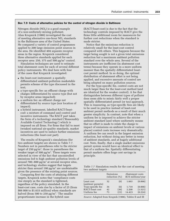
Pollution control: instruments 233
Box 7.9 Costs of alternative policies for the control of nitrogen dioxide in Baltimore
(RACT/least-cost) is due to the fact that thetechnology controls imposed by RACT give thefirms little additional room for manoeuvre forfurther cost reductions when the standard ismade stricter.
Notice that the emissions reduction isrelatively small for the least-cost controlcompared with others. This happens because thetarget being sought is not a given total emissionsreduction but a maximum ambient pollutionstandard over the whole area. Several of theinstruments are inefficient (in abatement costterms) because they operate in a more uniformmanner than the spatially differentiated least-cost permit method. In so doing, the optimaldistribution of abatement effort is not beingapplied, and excessive amounts of control arebeing adopted on many pollution sources.
For the type-specific fee, control costs are notmuch larger than for the least-cost method (andare identical for the weaker control). A fee thatdistinguishes between different types of polluterdoes seem able to mimic fairly well a properspatially differentiated permit (or tax) approach.This is reassuring, as type-specific fees are likelyto be used in practice instead of least-costambient permit methods as a result of their muchgreater simplicity. In contrast, note that when auniform fee is imposed to achieve the stricterambient standard (and where uniformity meansthat no effort is made to relate the charge toimpact of emissions on ambient levels at variousplaces) control costs increase very dramatically.A uniform fee can result in the largest emissionreduction, but without doing any better in termsof ambient standards, and at hugely additionalcost. Note, finally, that a single market emissionspermit system would have an identical effect tothat of a uniform fee. Spatially differentiatingpermit markets offers huge cost savings inprinciple.
Nitrogen dioxide (NO2) is a good example of a non-uniformly-mixing pollutant. Alan Krupnick (1986) investigated the cost of meeting alternative one-hour NO2 standards in the Baltimore area of the United States. He compared a variety of control programmesapplied to 200 large emission point sources inthe area. He identified 404 separate receptorareas in the region. Krupnick considered three alternative standards applied for eachreceptor area: 250, 375 and 500 µg/m3 control.
Simulation techniques are used to estimatetotal abatement costs for each of several differentpolicy instruments. We deal here with four of the cases that Krupnick investigated:
n the least-cost instrument: a spatiallydifferentiated ambient-pollution marketablepermits scheme of the type discussed in thetext;
n a type-specific fee: an effluent charge withcharges differentiated by source type (but notby receptor areas impacted);
n a uniform fee: an effluent charge notdifferentiated by source type (nor location ofimpact);
n a hybrid instrument, labelled RACT/least-cost: a mixture of command and control andincentive instruments. The RACT part takesthe form of a technology standard (‘ReasonablyAvailable Control Technology’) which isimposed on all firms. For firms that fail to meet(weaker) national air-quality standards, marketincentives are used to induce further emissionsreductions (the least-cost part).
The results of Krupnick’s simulations (for two ambient targets) are shown in Table 7.7.Numbers not in parentheses refer to the strictertarget of 250 µg/m3, those in parentheses theweaker target of 500 µg/m3. These targets wereselected in view of the fact that uncontrolledemissions led to high ambient pollution levels ofaround 700–800 µg/m3 at several receptor sites,and technology studies suggest that targetsstricter than around 190 µg/m3 are unobtainablegiven the presence of the existing point sources.
Comparing first the costs of attaining differenttargets, Krupnick notes that ‘compliance costsrise steeply as the standard is tightened,regardless of the policy simulated. In the least-cost case, costs rise by a factor of 25 (from$66 000 to $1.633 million) when standards arehalved (from 500 to 250 µg/m3.’ The smallerproportionate increase in the hybrid case
Table 7.7 Simulation results for the cost of meetingtwo ambient targets
Emissions Abatement costsreduction (%) $US millions/year
Least cost 32 (6) 1.663 (0.066)(ambient permits)Type-specific fee 34 (6) 1.719 (0.066)RACT/least cost 42 (36) 2.200 (1.521)Uniform fee 73 (21) 14.423 (0.224)
Source: Adapted from Krupnik (1986), Tables II and III

234 Environmental pollution
lated for each firm that will equalise marginal abate-ment costs. It is very unlikely that this requirementwill be met. The conclusion we draw from this isthat a command and control quantity regulationapproach is inefficient relative to a tax, subsidy ormarketable permit scheme, and so will achieve anyspecified target at a higher real cost. Some empiricalevidence on this is presented in Box 7.10.
For a non-UMP, the remarks above need to bequalified. Cost-effective command and control sys-tems, as before, require knowledge of individualfirms’ marginal cost of abatement functions. But sotoo do tax and subsidy instruments in this case. Ingeneral, only transferable permit schemes do notrequire that knowledge. This accords permit systemsgreat potential advantages over others.
7.6.2 Monitoring, administering andenforcing compliance costs
Little or nothing has been said so far about the costs associated with monitoring, administering andenforcing compliance for each instrument. Yet these
7.6 A comparison of the relative advantages of command and control, emissions tax, emission abatement subsidy and marketable permit instruments
In this section, we bring together a set of resultsobtained earlier in the chapter, and introduce a fewadditional results; all these are of benefit in assess-ing the relative merits of alternative pollution con-trol instruments.
7.6.1 Cost-efficiency
We established earlier several results relating tocost-efficiency. To summarise, an emissions tax,emissions abatement subsidy or marketable permitsystem can achieve any emissions target at leastcost. A command and control (CAC) regulationinstrument may, but will not usually, be cost-efficient. In order to be cost-efficient, the EPA mustknow each polluter’s marginal cost of abatementfunction so that an emission control can be calcu-
Box 7.10 The costs of emissions abatement using command and control and market-based instruments
A substantial literature now exists on thecomparative costs of attaining emissionsabatement targets using traditional quantity ortechnology regulations – what we call commandand control (CAC) instruments – and so-calledmarket instruments (particularly emissions taxes,abatement subsidies and marketable/transferableemissions permits). Much of this literaturederives from experience in the USA with thesetwo categories of instrument. Tietenberg (1990)provides an admirable account of recentevidence on these costs. Table 7.8 reproducesone of Tietenberg’s tables, showing the ratio ofcosts under CAC approaches to the least-costcontrols (using market instruments) for airpollution control in the United States. We have examined one of these studies – that byKrupnick (1986) – in more detail in Box 7.9.
Although they can be ‘best’ instruments insome circumstances, such direct controls areoften extremely costly. Tietenberg (1984) findsthat the CAC approach costs from twice to 22
times the least-cost alternative for given degreesof control. These ratios suggest that massive costsavings might be available if market instrumentswere to be used in place of CAC. In his 1990paper, Tietenberg reports estimates thatcompliance with the US Clean Air Act throughmarket instruments has led to accumulatedcapital savings of over $10 billion. It should bepointed out, however, that most studies compareactual CAC costs with those theoreticallyexpected under least-cost market-basedinstruments. In practice, one would not expectmarket instruments to operate at these theoreticalminimum costs, and so the ratios we quotedabove overstate the cost savings that would beobtained in practice by switching from CACtechniques.
Three arguments underlie the tenet thatmarket-based incentive approaches are likely to be more efficient than regulation and control.First, markets are effective in processinginformation; second, market instruments tend

Pollution control: instruments 235
to result in pollution control being undertakenwhere that control is least costly in real terms;and third, market-based approaches generatedynamic gains through responses over time totheir patterns of incentives.
However, stringent conditions are necessaryfor markets to guarantee efficient outcomes.Policy instrument choice takes place in a‘second-best’ world, where results are much lessclear. The absence of markets (including thosefor externalities and public goods), asymmetricinformation, moral hazard and other instances of market failure, all point to possible benefits of CAC-based public intervention or to theinappropriateness of complete reliance on
markets and market instruments. (See Fisher and Rothkopf (1989) for an excellent survey.)
A European example is given in the fileAgriculture.doc in the Additional Materialsfor Chapter 7. A study by Andreasson (1990)examines the real resource costs of threedifferent policies for reducing nitrate fertiliseruse on the Swedish island of Gotland: non-marketable quotas on fertiliser use, a tax onnitrogenous fertiliser and a marketable permitsystem. Some additional references to studieswhich attempt to quantify the costs of attainingpollution standards using various instrumentsare given in the recommendations for furtherreading.
Box 7.10 continued
Table 7.8 Empirical studies of air pollution control
Study Pollutants covered Geographic area CAC benchmark Ratio of CAC cost to least cost
Atkinson and Lewis Particulates St Louis SIP regulations 6.00a
Roach et al. Sulphur dioxide Four corners SIP regulations 4.25in Utah Colorado,
Arizona, andNew Mexico
Hahn and Noll Sulphates standards Los Angeles California emission 1.07Krupnick Nitrogen dioxide Baltimore Proposed RACT 5.96b
regulationsSeskin et al. Nitrogen dioxide Chicago Proposed RACT 14.40b
regulationsMcGartland Particulates Baltimore SIP regulations 4.18Spofford Sulphur dioxide Lower Delaware Uniform percentage 1.78
Valley regulationsParticulates Lower Delaware Uniform percentage 22.0
Valley regulationsHarrison Airport noise United States Mandatory retrofit 1.72c
Maloney and Hydrocarbons All domestic Uniform percentage 4.15d
Yandle DuPont plants reductionPalmer et al. CFC emissions United States Proposed 1.96
from non-aerosol standardsapplications
Notes:CAC = command and control, the traditional regulatory approach.SIP = state implementation plan.RACT = reasonably available control technologies, a set of standards imposed on existing sources in non-attainment areas.a Based on a 40 µg/m3 at worst receptor.b Based on a short-term, one-hour average of 250 µg/m3.c Because it is a benefit–cost study instead of a cost-effectiveness study the Harrison comparison of the commandand control approach with the least-cost allocation involves different benefit levels. Specifically, the benefit levels associated with the least-cost allocation are only 82% of those associated with the command-and-controlallocation. To produce cost estimates based on more comparable benefits, as a first approximation the least-costallocation was divided by 0.82 and the resulting number was compared with the command-and-control cost.d Based on 85% reduction of emissions from all sources.Source: Tietenberg (1990), Table 1

236 Environmental pollution
costs could be quite substantial. If they are large, and if they differ significantly between instruments,these costs are likely to have an important bearingon which type of instrument is least-cost for achiev-ing some target. One reason for the prevalence ofminimum technology requirements as a pollutioncontrol instrument may be that these costs are lowrelative to those of instruments that try to regulateemissions output levels.
7.6.3 Long-run effects
From the point of view of the EPA, instrument selec-tion will depend on the degree to which the amountof pollution control varies with the passage of timefor any particular instrument. An important consid-eration concerns whether or not the long-run effectis markedly different from the short-run effect. Thelong-run effect of an instrument depends mainly ontwo things: net income effects and technologicalinnovation effects. We consider each of these in turn.
Net income effects
Changes in net income arising from the operation ofa pollution control instrument can affect the long-run industry size. We noted earlier that subsidyschemes may have the (environmentally) undesir-able property of increasing the long-run size of thetargeted industry through positive income effects.Similar issues were raised when we were comparingalternative methods of initially allocating market-able permits.
Of course, it is possible in principle to design con-trol regimes that are revenue-neutral. For example,firms in a subsidised industry may be required tomake lump-sum payments which sum to the totalvalue of subsidies. This would preserve the incent-ive effects of subsidy systems without allowinglong-run effects arising from income changes. How-ever, it may be politically difficult to implementsuch a scheme, and there may be reasons why gov-ernment does not wish to match receipts and pay-ments in such a way.
Technology effects
A second route through which long-run effects maytransmit is via induced impacts on the rate of tech-
nological innovation. There are two aspects to this.One concerns what are sometimes called dynamicefficiency effects. These arise from the pattern ofincentives to innovate generated by a pollution con-trol instrument. A common argument in this regardis that command and control instruments have poorlong-run properties because they generate weakincentives for innovation (see, for example, Jaffeand Stavins, 1994). The binary nature of many suchinstruments (you reach the target or you do not reachit) creates a discrete switch in behaviour: once arequired target has been obtained there is no longerany incentive to go further.
In contrast (it is argued) an emissions tax (orabatement subsidy) will generate a dynamically effi-cient pattern of incentives on corporate (and con-sumer) behaviour. The incentive structure operatesto continually reward successful environmentallyfriendly innovation. In a market-based scheme, everyunit of emissions reduction is rewarded by a tax saving. The key issue here is what incentives firmsface in developing pollution-saving technology ordeveloping new, environmentally cleaner products.Under a emissions tax scheme, these incentives maybe strong, as we show in Figure 7.9.
Area Ω is the saving that would result if mar-ginal costs were lowered from MC1 to MC2 and theemissions level were unchanged. But if marginalcost were lowered in this way, the firm’s profit-maximising emissions abatement level would risefrom Z1* to Z2*, and so an additional saving of Λwould accrue to the firm. The firm has an incentive
Figure 7.9 Dynamic incentives under emissions taxcontrols

Pollution control: instruments 237
to develop new technology to abate emission if thetotal costs of developing and applying the techno-logy are less than the present value of the savings Ω + Λ accumulated over the life of the firm.19 In contrast, in a CAC regulatory system, dynamic incent-ives are weaker or non-existent. As we said above, if a target is set in (non-marketable) quantitativeterms, then once that target has been met there is little or no further incentive on the polluter to reduceemissions.
But there is a second aspect that weakens theforce of these arguments. Some researchers believethat technological change can be driven from above.Suppose that the EPA identifies best-practice envir-onmentally friendly technology, and imposes this asa requirement on firms through minimum acceptabletechnology regulations. Not only will this have adirect effect on spreading technology diffusion, butthe indirect effects may be powerful too. Barriersdue to frictions, lack of information, and other mar-ket imperfections that may lead firms to be over-cautious or unable to act voluntarily no longer bite inthe face of imposed requirements. Moreover, thesechanges have catalytic effects which set in motionspurts of innovation as learning effects occur. Thesekinds of arguments are likely to have most relevancefor technological innovation and diffusion in devel-oping economies.
It is difficult to arrive at unequivocal conclusionsfrom all this. However, a reasonable conclusion mustbe that, in some circumstances at least, technology-based controls and other command and controlinstruments will have superior long-run properties tomarket-based instruments.
7.6.4 Double dividend
In the previous chapter, we noted the possibility thatsome environmental regulation schemes may gen-erate a so-called double dividend. It seems likelythat the availability and size of a double dividendwill vary from one circumstance to another, and onwhich instrument is being used. A sensible choice ofinstrument should consider these matters.
7.6.5 Equity/distribution
Finally, we note that the distributional consequencesof a pollution control policy instrument will be veryimportant in determining which instruments areselected in practice. Different instruments for pollu-tion control have different implications for the dis-tribution of income within an economy. We havealready examined the direct business financial gainsand losses (which are, of course, exactly mirrored by offsetting government financial losses or gains).It is also necessary to think about the consequencesfor income and wealth distribution in society as awhole. For example, an emissions tax imposed uponfossil fuels will indirectly affect final consumerswho purchase goods that have large energy input.Individuals for whom heating comprises a large pro-portion of their budget may well experience quitelarge falls in real income. Indeed, many kinds of‘green taxes’ are likely to have regressive effectsupon income distribution.
It is important to distinguish between incomeshifts that are merely redistributive and do not cor-respond to any real resource gains and losses to theeconomy, and real income changes which do implyreal resource changes for the economy as a whole.The latter arise because pollution control doesinvolve real costs. Of course, by having less pollu-tion, there are benefits to be had as well, which in awell-designed pollution control programme shouldoutweigh these real costs. Nevertheless, the bene-ficiaries and losers will not be the same individuals,and it is this that one is concerned with when dis-cussing the equity or fairness of an instrument.
It should also be noted that emissions taxes (and other environmental controls) have importantimplications for the relative competitiveness ofnational economies. (See Chapter 10 for more onthis.) Some analysts have advocated a switch fromtaxes on labour and capital to taxes on emissions toavoid excessive tax burdens, and schemes have beenproposed to penalise nations that attempt to gaincompetitive advantage by not introducing emissionstaxes. Good discussions of these issues are to be
19 Note that the optimal tax rate would change as new technology lowers control costs, so matters are a little more complicated.
Summary
• An instrument that attains a pollution target at least cost is known as a cost-effective instrument.• A least-cost control regime implies that the marginal cost of abatement is equalised over all firms
undertaking pollution control.• Bargaining processes might bring about efficient outcomes (and so might lead to the attainment of
targets without regulatory intervention).• The likelihood of efficient bargaining solutions to pollution problems being achieved is reduced by
the presence of bargaining costs, and if bargaining would take place over a public (as opposed to aprivate) good.
• Pollution control instruments can be classified into a set of broad classes, the most important ofwhich are command and control instruments and economic incentive-based instruments.
• In many – but not all – circumstances, economic incentive-based instruments are more cost-effective than command and control instruments.
• The long-run effects of pollution control instruments can be very different from their short-runeffects, because of net income effects and impacts on the rate and direction of technologicalchange.
• Where a pollutant is not uniformly mixing, the relative advantages of incentive-based instrumentsare considerably reduced. Some forms of marketable permit systems appear to offer the bestprospect of attaining ambient pollution targets cost-effectively.
• Our discussion of the properties and relative advantages of various instruments that could be usedto attain environmental policy targets has taken place under the implicit assumption that somesingle authority has the ability to implement and administer a control programme. But manypollution problems spill over national boundaries. Given that the world does not have a singlegovernment, how can policy targets and instruments be devised, introduced, administered andmonitored for global or international pollution problems? This question warrants separate attentionin Chapter 10.
238 Environmental pollution
found in Bertram et al. (1989), Brown (1989),Grubb (1989a), Hansen (1990), Kosmo (1989) andWeizsäcker (1989).
As we noted earlier, where a particular instrumenthas an adverse financial effect on one sector of theeconomy, it is open to the government to use com-pensating fiscal changes to offset those changes sothat the distribution of income and wealth betweenindividuals is not systematically changed. For exam-ple, the financial transfers implied by a emissionstax scheme could be compensated by lump-sumpayments to firms or by abatement subsidy pay-ments. And income transfers from poorer groupsfacing higher energy bills, for example, could becompensated for by other fiscal changes.
The main point here is that additional tax rev-enues received by government could be distributedto groups adversely affected by the initial policychange. However, the difficulties in designing dis-tributionally neutral packages are immense. Wherecompensation is paid to individuals or groups forwhom the tax incidence is considered excessive, the form of compensation should be designed not toalter behaviour, otherwise the efficiency propertiesof the instrument will be adversely affected. Thisimplies lump-sum compensation should be usedwhere possible. Compensation schemes of this formrarely happen in practice. Nevertheless, decisionmakers do have this option; whether they choose toexercise it is another matter.
Pollution control: instruments 239
Further reading
EEA (2000), an online survey of environmentaltaxes in the EU.
Pearce and Brisson (1993) discuss the use of command and control instruments in the UK. Bohm(1981) considers deposit refund systems. Helm(1993, 1998) discusses possible reform of environ-mental regulation in the UK. Smith (1998) invest-igates taxation of energy. Portney (1990) analyses air pollution policy in the USA, and Portney (1989)assesses the US Clean Air Act. Crandall (1992) provides an interesting analysis of the relativeinefficiency of a standards-based approach to fuelefficiency in the United States. Kolstad (1987)examines the inefficiency losses associated withusing undifferentiated taxes or other charges wheneconomic efficiency requires that charges be differ-entiated across sources. Krupnick’s (1986) paper onnitrogen dioxide control in Baltimore, discussed inthe chapter, repays reading in the original.
Dales (1968) is the paper generally credited withhaving established the notion that marketable permits may be used for pollution control, andMontgomery (1972) derived the efficiency proper-ties of marketable permits. For accounts of the useof market-based pollution control instruments seeHahn (1984, 1989), Hahn and Hester (1989a, b),Opschoor and Vos (1989) and Tietenberg (1990,1992). Jorgensen and Wilcoxen (1990a, b, c) ana-lyse the impact of environmental regulation uponeconomic growth in the United States (but note thatthese papers are relatively difficult).
The following references deal with air pollu-tion emissions trading programmes in developingcountries: Ellerman (2001), SO2 emissions in China;Blackman and Harrington (1999); Benkovic andKruger (2001); Montero et al. (2000), Chile; andseveral papers in the Journal of Economic Per-spectives (Summer 1998, Vol. 12, no 3). Somegeneral accounts of air emissions problems andpolicies in India are found in Bose et al. (1997,1998). Cowan (1998) considers the use of economicinstruments for water pollution and abstraction.
Enforcement issues and incentive compatibility(to be discussed in the next chapter) are analysed inHeyes (1998) and Laplante and Rilstone (1996). For
Where a reference is underlined below, it is avail-able online; the URL is given in the References.
Baumol and Oates (1988) is a classic source in thearea of environmental regulation. The whole book is relevant but it is quite difficult and formal. Thetheoretical basis for a political economy of environ-mental regulation is investigated in Boyer and Laffont(1999). Tietenberg (1992, chapters 14 to 20) providesan extensive and primarily descriptive coverage ofspecific types of pollution and the control techniquesapplied to each. Other good general accounts of pol-lution control policy are to be found in Fisher (1981,chapter 12), which discusses the work of RonaldCoase and the roles of wealth and bargaining power,Common (1995), Hartwick and Olewiler (1986) andGoodstein (1995). Fisher and Rothkopf (1989) con-sider the justification for public policy in terms ofmarket failure. A possibility, that we touch upon inthe next chapter, is that public intervention itself gen-erates substantial costs. These costs may be suffici-ently large to prevent intervention delivering positivenet benefits. This notion of ‘government failure’ isanalysed in Weimer and Vining (1992). Laffont andTirole (1993, 1996) discuss the innovation incentiveeffects of permits when number is limited.
There are several national and international agen-cies that produce periodic surveys of environmentalprotection instruments and their effectiveness.Among these are various parts of the United NationsOrganisation, the European Union, the United StatesEPA and the OECD. An extensive listing can befound on the Chapter 7 Links web page. Referencesthat the reader may find useful include OECD(1995), which surveys the use of environmentaltaxes and other charges used for environmental protection in the OECD countries; Anderson et al.(1997), US experience with economic incentivesinstruments; OECD (1997d), evaluating economicinstruments for environmental policy; OECD (1999)for a detailed account of instruments used – and theireffectiveness – in OECD countries; EPA (1999),economic incentives for pollution control in theUSA; EPA (2001), US experience with economicincentives; EEA (2001), which considers ways ofimproving official environmental reporting; and

Ribaudo et al. (1999), and for non-point pollutionfrom agriculture Vatn et al. (1997).
Useful accounts of instruments used in fisheriesmanagement include OECD (1997c) and the regularOECD publication Review of Fisheries, whichcovers changes in fishery management systems.Discussion of the idea of a safe minimum standardof conservation can be found in Bishop (1978) andRandall and Farmer (1995). The ‘Blueprint’ series(see, for example, Pearce, 1991a) provides a clearand simple account of the new environmental eco-nomics policy stance, in a rather ideological style.Finally, a number of texts provide collections ofpapers, several of which are relevant to pollutioncontrol policy: these include Bromley (1995) and, ata more rigorous level, the three ‘Handbooks’ editedby Kneese and Sweeney (1985a, b, 1993).
240 Environmental pollution
a detailed analysis of issues concerning compensa-tion in connection with distribution effects of taxchanges, see Hartwick and Olewiler (1986, chapter12), who also analyse the consequences of subsidiesand taxes in the short run and the long run. The roleand importance of non-convexities are discussed in Fisher (1981, p. 177), Portes (1970) and Baumoland Oates (1988). Second-best aspects of taxation,and possible double dividends from environmental policy, are discussed in Cremer and Gahvani (2001)and Parry et al. (1999).
The seminal text on non-point pollution is Russelland Shogren (1993). Others on this topic includeDosi and Tomasi (1994), Braden and Segerson(1993), Laffont (1994), Millock et al. (1997),Romstad et al. (1997), Segerson (1988) and Shogren(1993). For water pollution see Segerson (1990) and
Discussion questions
1. Suppose that the EPA obtains damages frompolluting firms in recompense for the damagecaused by the pollution. Should the EPAdistribute the moneys recovered from suchdamage settlements to the pollution victims?(Hint: consider, among other things, possiblechanges in victim behaviour in anticipation ofsuch compensation.)
2. Consider a good whose production generatespollution damage. In what way will the effectsof a tax on the output of the good differ fromthat of a tax on the pollutant emissionsthemselves? Which of the two is likely to beeconomically efficient? (Hint: think aboutsubstitution effects on the demand side and on the supply side.)
3. Evaluate the arguments for the use of marketor incentive-based instruments versus‘command and control’ instruments in theregulation of environmental externalities underconditions of certainty.
4. Discuss the scope for the allocation of privateproperty rights to bring the privately andsocially optimal levels of soil pollution intoline.
5. Discuss the distributional implications of different possible methods by whichmarketable permits may be initially allocated.
6. Distinguish between private and public goods externalities. Discuss the likelihood ofbargaining leading to an efficient allocation ofresources in each case.
7. Use diagrams to contrast pollution taxinstruments with marketable emission permitsystems, paying particular attention to thedistributional consequences of the two formsof instrument. (Assume a given, target level of pollution abatement, and that permits areinitially distributed through sale in acompetitive market.)
8. Discuss the efficiency properties of a pollutiontax where the tax revenues are earmarked inadvance for the provision of subsidies for theinstallation of pollution abatement equipment.
9. Suppose that a municipal authority hires a firmto collect and dispose of household waste. Thefirm is paid a variable fee, proportional to thequantity of waste it collects, and is charged a

Pollution control: instruments 241
fee per unit of waste disposed at a municipalwaste landfill site. Households are not chargeda variable fee for the amount of waste theyleave for collection, instead they pay an annualfixed charge. Comment on the economicefficiency of these arrangements and suggesthow efficiency gains might be obtained.
10. An interesting example of a regulatory failurerelates to electricity generating stations in the UK. Several thermal power stations in the UK were required to install flue-gasdesulphurisation (FGD) plant in order to meet
a national standard for sulphur emissions. The power stations fitted with FGD plant are not compensated for sulphur abatement.Electricity is purchased for the national grid on a competitive bidding system. The stationsfitted with FGD are unable to compete on costwith other stations without that equipment, andas a result are withdrawn entirely from the gridat some times and operate below capacity atothers.
Explain why this situation is sociallyinefficient, and suggest a means by which this inefficiency could be avoided.
Problems
1. Suppose that an EPA must select oneinstrument from two available. Two criteriamatter: (a) P, the probability of the instrumentattaining its target; (b) C, the proportionatesaving in abatement cost incurred in using that instrument (relative to the cost using thehighest-cost instrument). The EPA calculates aweighted sum (score) for each instrument, andchooses that with the highest score. Assumethat the instruments have the following valuesfor P and C:
Instrument 1: P = 0.9, C = 0.0
Instrument 2: P = 0.7, C = 0.2
(i) Write an Excel spreadsheet to illustrate howthe instrument choice varies with changes inthe relative weights (between zero and one)attached to the two criteria. Also explorehow instrument choice varies as themagnitudes of P and C for each instrumentvary.
(ii) Use an algebraic formulation of thisproblem to obtain expressions that allowthese results to be shown analytically.
2. Using the Excel workbook Leastcost.xls,demonstrate that the cost penalty from sharingabatement equally between the two firms ratherthan using the least-cost distribution ofabatement is larger the greater is the difference
in the firms’ abatement cost functions (asmeasured by the value of the slope parameterin the abatement cost functions).
3. The Coase theorem claims that a unique andefficient allocation of resources would followfrom rational bargaining, irrespective of howproperty rights were initially allocated.Demonstrate that the distribution of net gainsbetween bargaining parties will, in general,depend upon the initial distribution of propertyrights.
4. Show that a pollution tax on emissions and a subsidy to output producers for each unit of pollution reduction would, if the rates ofsubsidy were identical to the pollution tax rate, lead to identical outcomes in terms of thelevels of output and pollution for a given sizedindustry. Explain why the distribution of gainsand losses will usually differ, and why thelong-run level of pollution abatement maydiffer when the industry size may change.
5. In all discussions of pollution abatement costsin this chapter, the fixed costs of pollutionabatement were implicitly taken to be zero. Do any conclusions change if fixed costs arenon-zero?
6. Demonstrate that in the simple special case ofa uniformly mixing flow pollutant, in whichthe value of the damage created by the

242 Environmental pollution
emission is independent of the location of theemission source or the time of the emission,the tax rate should be uniform over allpolluters for the tax to be an efficientinstrument (that is, it will be applied at thesame rate per unit of pollution on all units ofthe pollutant).
7. Our discussion in this chapter has shown that if the control authority does not know themarginal damage function, it will not be ableto identify the economically efficient level ofpollution abatement, nor the efficient tax orsubsidy level. Demonstrate that(a) knowledge of the pollution abatement
schedule alone means that it can calculatethe required rate of tax to achieve anytarget level it wishes,
(b) if it knew neither the marginal damage northe marginal abatement cost schedules, thenit could arbitrarily set a tax rate, confidentin the knowledge that whatever level ofabatement this would generate would beattained at minimum feasible cost.
8. You are given the following information:(a) A programme of air pollution control
would reduce deaths from cancer from 1 in 8000 to 1 in 10 000 of the population.
(b) The cost of the programme is expected to lie in the interval £2 billion (£2000million) to £3 billion annually.
(c) The size of the relevant population is 50 million persons.
(d) The ‘statistical value’ of a human life isagreed to lie in the interval £300 000 to £5 million.
If the only benefit from the programme isthe reduced risk of death from cancer, canthe adoption of the programme be justifiedusing an economic efficiency criterion?
9. In controlling emissions, there is an importantdifference between a command and controlinstrument and a tax instrument. Both requirethat the polluter pay the cost of attaining theemission reduction target. However, the taxinstrument imposes an additional charge (on the emissions which remain at the targetlevel of pollutions); this is not paid under acommand and control regime. The failure to incorporate damage costs into the price of the product can generate distortions orinefficiencies in the economy. Kolstad (2000),from which this problem is drawn, gives anexample in the paper manufacturing industry.Suppose that paper can be produced using pulp either from recycled paper (which is non-polluting) or from virgin timber (which is polluting). Compare the operation of a CACinstrument with a tax instrument applied to themanufacture of pulp from virgin timber, andshow how this distorts (creates an inefficiency)in paper production.
10. This exercise involves using an Excel file to undertake some simulations regarding the relative costs of alternative instruments, and to interpret and comment on your results.Instructions for the exercise are given inPollution2.doc; the Excel file is Pollution2.xls.Both of these can be found in the AdditionalMaterials for Chapter 7.
Appendix 7.1 The least-cost theorem and pollution control instruments
This appendix is structured as follows. In Part 1, wedefine the notation used and set the scene for whatfollows. Then in Part 2 we derive a necessary condi-tion for pollution control to be cost-effective: that is,to attain any given target at least cost. An EPA hasseveral instruments available for attaining a pollu-tion (or pollution abatement) target. Here we con-
sider three classes of instrument: quantitative regu-lations (a variant of command and control) in Part 3;an emissions tax (Parts 4 and 5); an emissions abate-ment subsidy (Part 6); and transferable emissionspermits (Part 7). Collectively, Parts 3 to 7 take thereader through what an EPA would need to know,and how it could operate each of those instruments,
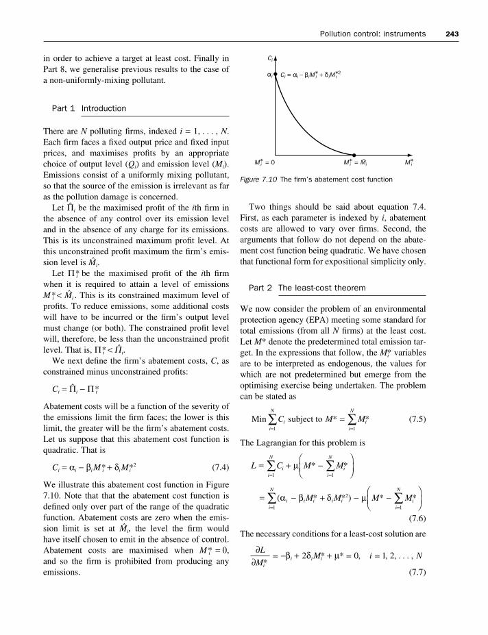
Pollution control: instruments 243
in order to achieve a target at least cost. Finally inPart 8, we generalise previous results to the case ofa non-uniformly-mixing pollutant.
Part 1 Introduction
There are N polluting firms, indexed i = 1, . . . , N.Each firm faces a fixed output price and fixed inputprices, and maximises profits by an appropriatechoice of output level (Qi) and emission level (Mi).Emissions consist of a uniformly mixing pollutant,so that the source of the emission is irrelevant as faras the pollution damage is concerned.
Let 6i be the maximised profit of the ith firm inthe absence of any control over its emission leveland in the absence of any charge for its emissions.This is its unconstrained maximum profit level. Atthis unconstrained profit maximum the firm’s emis-sion level is !i.
Let Π*i be the maximised profit of the ith firmwhen it is required to attain a level of emissions M*i < !i . This is its constrained maximum level ofprofits. To reduce emissions, some additional costswill have to be incurred or the firm’s output levelmust change (or both). The constrained profit levelwill, therefore, be less than the unconstrained profitlevel. That is, Π*i < ^i.
We next define the firm’s abatement costs, C, asconstrained minus unconstrained profits:
Ci = 6i − Π*i
Abatement costs will be a function of the severity ofthe emissions limit the firm faces; the lower is thislimit, the greater will be the firm’s abatement costs.Let us suppose that this abatement cost function isquadratic. That is
Ci = αi − βiM*i + δiMi*2 (7.4)
We illustrate this abatement cost function in Figure7.10. Note that that the abatement cost function isdefined only over part of the range of the quadraticfunction. Abatement costs are zero when the emis-sion limit is set at !i, the level the firm would have itself chosen to emit in the absence of control.Abatement costs are maximised when M*i = 0, and so the firm is prohibited from producing anyemissions.
Two things should be said about equation 7.4.First, as each parameter is indexed by i, abatementcosts are allowed to vary over firms. Second, thearguments that follow do not depend on the abate-ment cost function being quadratic. We have chosenthat functional form for expositional simplicity only.
Part 2 The least-cost theorem
We now consider the problem of an environmentalprotection agency (EPA) meeting some standard fortotal emissions (from all N firms) at the least cost.Let M* denote the predetermined total emission tar-get. In the expressions that follow, the Mi* variablesare to be interpreted as endogenous, the values forwhich are not predetermined but emerge from theoptimising exercise being undertaken. The problemcan be stated as
(7.5)
The Lagrangian for this problem is
(7.6)
The necessary conditions for a least-cost solution are
(7.7)
∂∂
β δ µL
MM i N
ii i i
* * * , , , . . . , = − + + = =2 0 1 2
M M M Mii
N
i i i i ii
N
( * * ) * *= − + − −
= =∑ ∑
1
2
1
α β δ µ
L C M Mii
N
ii
N
* * = + −
= =∑ ∑
1 1
µ
Min subject toC M Mii
N
ii
N
= =∑ ∑=
1 1
* *
Figure 7.10 The firm’s abatement cost function
244 Environmental pollution
and
(7.8)
Equations 7.7 and 7.8 give N + 1 equations in N + 1 unknowns. Solving these simultaneously giveseach firm’s emission limit, M*i (which now should be regarded as the optimised emissions limit for thefirm), and the optimised shadow price of the pollu-tion constraint (the Lagrange multiplier) µ*. Sinceµ* is constant over all firms, it can be seen fromequation 7.7 that a least-cost pollution abatementprogramme requires that the marginal cost of abate-ment be equal over all firms.
There is a tricky issue relating to signs in equa-tion 7.7. Notice that an increase in M*i corresponds to a relaxation of a pollution target (a decrease inrequired abatement) so the term (−βi + 2δi M*i) is themarginal cost of a reduction in pollution abatementbeing required of firm i. It will therefore be a negat-ive quantity. This can be verified by looking at theslope of the Ci function in Figure 7.10.
By multiplying equation 7.7 through by minusone, we obtain
βi − 2δi M*i = µ* (7.7′)
Here the term on the left-hand side (βi − 2δiM*i ) is the firm’s marginal cost of an increase in pollu-tion abatement, a positive quantity. It follows from7.7′ that µ* is also a positive quantity. This is consistent with the text of this chapter and the pre-vious one, and matches, for example, the graphic inFigure 7.4.
Part 3 Least-cost pollution control usingquantitative regulation
If the EPA knew each firm’s abatement cost function(that is, it knew Ci for i = 1, . . . , N), then for anytotal emission standard it seeks, M*, the system ofequations 7.7 and 7.8 could be solved for M*ifor each firm. The EPA could then tell each firm howmuch it could emit. The total quantity of emissionswould, from equation 7.8, be reached exactly, andthe target would, as the above theorem shows, beattained at least cost.
∂∂µ
LM Mi
i
N
* * = − + ==∑
1
0
Part 4 Least-cost pollution control using anemissions tax
As an alternative to setting quantitative emissionscontrols on each firm, an emission tax could be used.If the EPA knew each firm’s abatement cost func-tion, then for any total emission standard it seeks,M*, the system of equations 7.7 and 7.8 could be solved for the value of the shadow price of thepollution constraint, µ*. Note that, unlike M*i , thisshadow price is constant for each firm. The EPAcould then set a tax at a rate of t* per unit of emis-sions and charge each firm this tax on each unit ofpollution it emitted. Profit-maximising behaviourwould then lead each firm to produce M*i emissions,the least-cost solution.
To see why this should be so, note that in theabsence of any quantity constraint on emissions,profit-maximising behaviour in the face of an emis-sions tax implies that the firm will minimise the sumof its abatement costs and pollution tax costs. Thatis, the firm chooses Mi to minimise CTi, the total ofits abatement and tax costs:
CTi = Ci + tMi = αi − βiMi + δiMi2 + t*Mi
The necessary condition is
(7.9)
Clearly, if t* in equation 7.9 is set equal to µ* inequation 7.7, the necessary conditions 7.7 and 7.9are identical, and so the tax instrument achieves thetotal emissions target at least cost.
Part 5 What role is there for a tax instrumentwhere each firm’s abatement costfunctions are not known?
In general, the EPA will not know abatement costs.However, if an arbitrarily chosen tax rate, say Y, isselected, and each firm is charged that rate on eachunit of emission, then some total quantity of emis-sions, say P, will be realised at least cost. Of course,that amount P will in general be different from M*.Only if Y = t* will P be identical to M*. An iterative,trial-and-error process of tax rate change may enablethe EPA to find the necessary tax rate to achieve aspecific target.
∂∂
β δCTi
ii i i
MM t i N * * , , , . . . , = − + + = =2 0 1 2

Pollution control: instruments 245
Part 6 Least-cost pollution control using anemissions-abatement subsidy
Another method of obtaining a least-cost solution toan emissions target is by use of abatement subsidies.Suppose a subsidy of s* is paid to each firm on eachunit of emissions reduction below its unconstrainedprofit-maximising level, !i. Then profit-maximisingbehaviour implies that the firm will maximise totalsubsidy receipts less abatement costs. That is, thefirm maximises
CSi = s(!i − Mi) − Ci = s(!i − Mi ) − (αi − βiMi + δiMi
2)
The necessary condition is
(7.10)
which, after multiplying through by −1, is identicalto equation 7.9 if s = t. So, once again, if s in equa-tion 7.10 is set equal to µ* in equation 7.7, the neces-sary conditions 7.7 and 7.10 are identical, and so the subsidy instrument achieves the total emissionstarget at least cost. Moreover, this result demon-strates that in terms of their effects on emissions, atax rate of t per unit of emissions is identical to asubsidy rate of s per unit of emissions abatement,provided s = t.
Part 7 Least-cost pollution control usingtransferable emissions permits
Suppose that the EPA issues to each firm licencespermitting L0
i units of emissions. Firms are allowedto trade with one another in permits. The ith firmwill trade in permits so as to minimise the sum ofabatement costs and trade-acquired permits:
CLi = Ci + P(Li − L0i )
= αi + βiMi + δiM2i + P(Li − L0
i ) (7.11)
where P is the market price of one emission permit.Given that Li is the quantity of emissions the firmwill produce after trade we can write this as
CLi = Ci + P(Li − L0i )
= αi − βi Li + δi Li2 + P(Li − L0
i ) (7.12)
The necessary condition for minimisation is
∂∂
β δCSi
ii i i
MM s i N * , , , . . . , = − − = =2 0 1 2
(7.13)
which can be interpreted as the firm’s demand func-tion for permits.
If the EPA sets a total emissions target of M* thenM* is the total supply of permits and
(7.14)
Now compare equations 7.13 and 7.14 with equa-tions 7.7 and 7.8. These are identical if P = µ*(remembering that Li = M*i ). Moreover, comparisonof equation 7.13 with equations 7.11 and 7.12 showsthat P = t = s. So by an initial issue of permits (dis-tributed in any way) equal to the emissions target,the EPA can realise the target at least cost. More-over, it can do so without knowledge of individualfirms’ abatement cost functions.
Part 8 Least-cost abatement for a non-uniformly-mixing pollutant
The target of the EPA is now in terms of ambientpollution levels rather than emission flows. Specific-ally the EPA requires that
(7.15)
The problem for the EPA is to attain this target atleast cost. We deal with the case where the sameambient target is set for each receptor area. Thisproblem can be stated as
for j = 1, . . . , J (7.16)
The Lagrangian for this problem is
(7.17)
where Ci = αi − βiMi + δiMi2
A d MJ Ji ii
N
* − −
=∑
1
µ
L C A d Mii
N
i ii
N
* . . . = − −
−
= =∑ ∑
11 1
1
µ
Min subject to *C A d M Aii
N
j ji ii
N
= =∑ ∑= ≤
1 1
A d M A j Jj ji ii
N
j= ≤ ==∑ * , . . . ,
1
1for
M LL
Lii
N
ii
N
* = = == =∑ ∑0
1 1
∂∂µ
∂∂
β δCLi
ii i i
LL P i N * , , , . . . , = − + + = =2 0 1 2

246 Environmental pollution
The necessary conditions for a least-cost solution are
i = 1, 2, . . . , N (7.18)
and
(7.19)
The system of equations 7.18 and 7.19 consists of N + J equations which can be solved for the N + Junknowns (M*i , i = 1, . . . , N and µj*, j = 1, . . . , J).
∂∂µ
LA d M j J
jji i
i
N
* , . . . , = − + = ==∑
1
0 1for
∂∂
β δ µL
MM d
ii i i j
j Jj ji
* ( * ) , = − + + ==
=∑2 01
Equation 7.18 can be written as
(7.20)
Then after multiplying through by −1, using MCi todenote the ith firm’s marginal cost of abatement, andexpanding the sum on the right-hand side, we obtain
MCi = µ1*d1i + µ2*d2i + . . . + µJ*dJi,i = 1, 2, . . . , N (7.21)
The pair of equations 7.20 and 7.21 can be comparedwith the solution for the uniformly mixing pollutioncase, equation 7.7 multiplied by −1.
− + = − ===∑β δ µi i i j
j Jj jiM d i N ( * ), , , . . . , 2 1 21


