NAVAL POSTGRADUATE SCHOOL MONTEREY, CALIFORNIA THESIS Approved for public release; distribution is unlimited PORTABLE SIGNALS ANALYSIS SOLUTIONS USING SIGNALWORKS®: A PROCESS GUIDE FOR ANALYSTS AND STUDENTS by Eric W. Sears September 2009 Thesis Co-Advisor: Tri Ha Thesis Co-Advisor: Vicente Garcia Second Reader: Raymond Elliott
Transcript
NAVAL
POSTGRADUATE SCHOOL
MONTEREY, CALIFORNIA
THESIS
Approved for public release; distribution is unlimited
PORTABLE SIGNALS ANALYSIS SOLUTIONS USING SIGNALWORKS®: A PROCESS GUIDE FOR ANALYSTS
AND STUDENTS
by
Eric W. Sears
September 2009
Thesis Co-Advisor: Tri Ha Thesis Co-Advisor: Vicente Garcia
Second Reader: Raymond Elliott
i
REPORT DOCUMENTATION PAGE Form Approved OMB No. 0704-0188 Public reporting burden for this collection of information is estimated to average 1 hour per response, including the time for reviewing instruction, searching existing data sources, gathering and maintaining the data needed, and completing and reviewing the collection of information. Send comments regarding this burden estimate or any other aspect of this collection of information, including suggestions for reducing this burden, to Washington headquarters Services, Directorate for Information Operations and Reports, 1215 Jefferson Davis Highway, Suite 1204, Arlington, VA 22202-4302, and to the Office of Management and Budget, Paperwork Reduction Project (0704-0188) Washington DC 20503. 1. AGENCY USE ONLY (Leave blank)
2. REPORT DATE September 2009
3. REPORT TYPE AND DATES COVERED Master’s Thesis
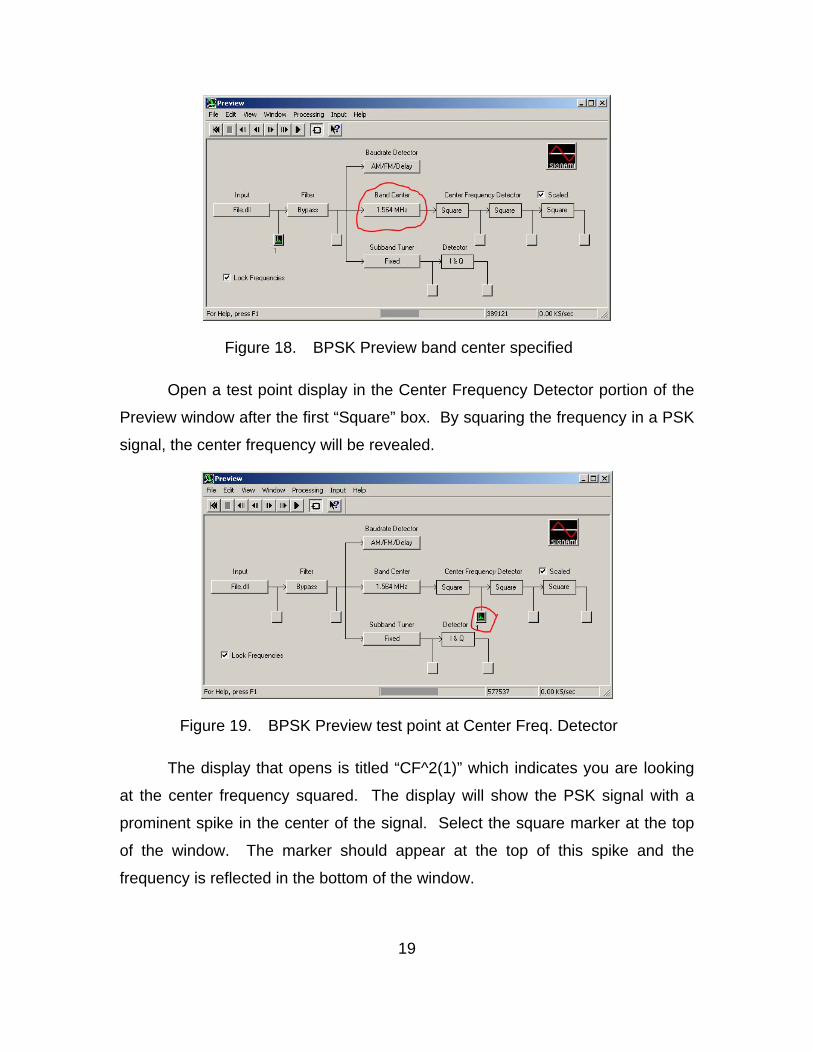
4. TITLE AND SUBTITLE Portable Signals Analysis Solutions using Signalworks®: A Process Guide for Analysts and Students 6. AUTHOR(S) LT Eric Sears
5. FUNDING NUMBERS
7. PERFORMING ORGANIZATION NAME(S) AND ADDRESS(ES) Naval Postgraduate School Monterey, CA 93943-5000
8. PERFORMING ORGANIZATION REPORT NUMBER
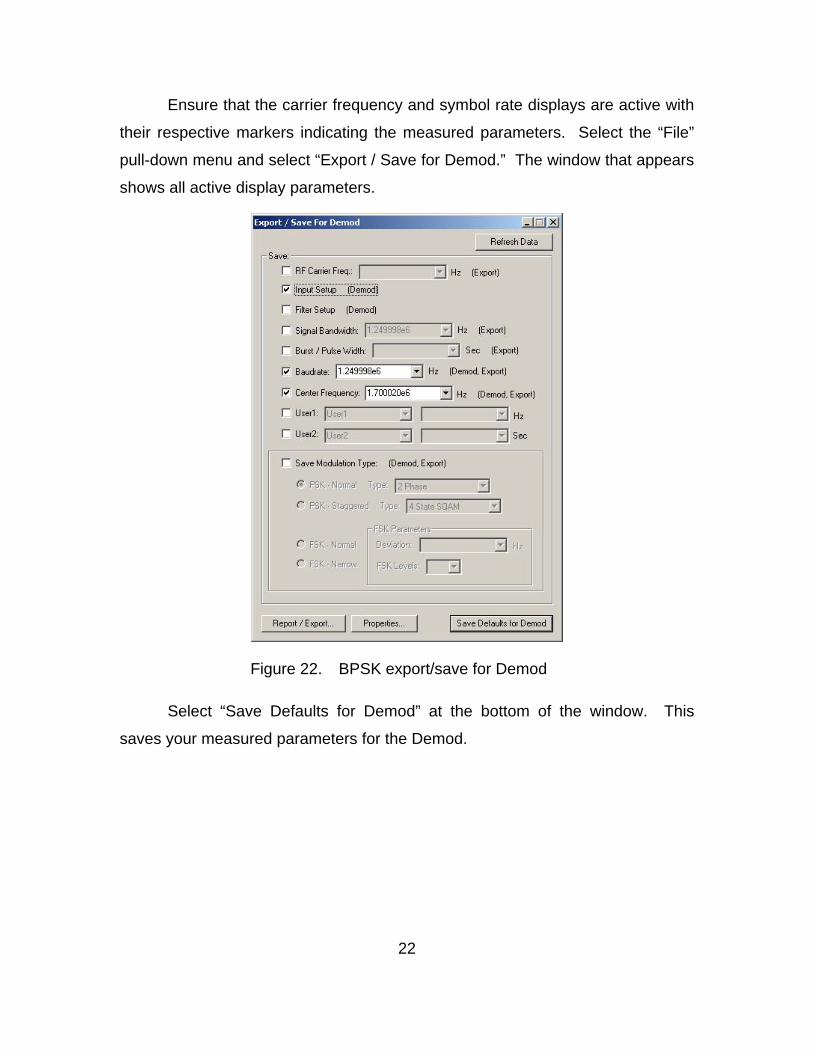
9. SPONSORING /MONITORING AGENCY NAME(S) AND ADDRESS(ES) N/A
10. SPONSORING/MONITORING AGENCY REPORT NUMBER
11. SUPPLEMENTARY NOTES The views expressed in this thesis are those of the author and do not reflect the official policy or position of the Department of Defense or the U.S. Government. 12a. DISTRIBUTION / AVAILABILITY STATEMENT Approved for public release; distribution is unlimited.
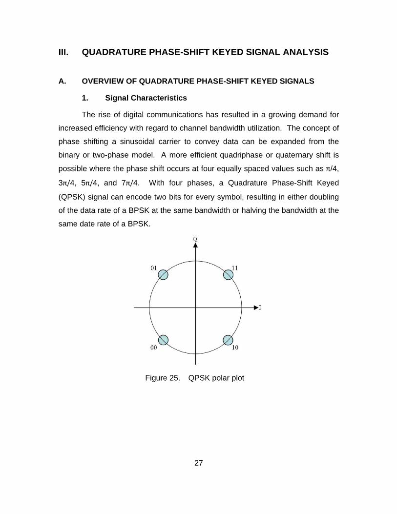
12b. DISTRIBUTION CODE
13. ABSTRACT (maximum 200 words) Signalworks® is a signals analysis software suite designed to be installed on Windows and Linux
portable computing platforms. The demodulation applications within the program offer considerable processing capability for a variety of signals coupled with a graphical interface that is both easy to use and configure. This thesis examines the process of building test signals within Signalworks® and then processing them with the available demodulation applications to define important parameters used to identify and analyze signals. Although Signalworks® version 4.0 is unable to demodulate Orthogonal Frequency Division Multiplexed (OFDM) signals often used in wireless communications, it can process Binary Phase-Shift Keyed (BPSK) and Quadrature Phase-Shift Keyed (QPSK) signals used in the 802.11b standard. While future versions may include OFDM demodulation capability, this analysis includes the feasibility of using Signalworks® in a lab environment to demonstrate and educate students on signal characteristics including wireless communication signals.
15. NUMBER OF PAGES
125
14. SUBJECT TERMS Signals analysis, portable signal processing, Signalworks®
16. PRICE CODE
17. SECURITY CLASSIFICATION OF REPORT
Unclassified
18. SECURITY CLASSIFICATION OF THIS PAGE
Unclassified
19. SECURITY CLASSIFICATION OF ABSTRACT
Unclassified
20. LIMITATION OF ABSTRACT
UU NSN 7540-01-280-5500 Standard Form 298 (Rev. 8-98) Prescribed by ANSI Std. Z39.18
ii
THIS PAGE INTENTIONALLY LEFT BLANK
iii
Approved for public release; distribution is unlimited.
PORTABLE SIGNALS ANALYSIS SOLUTIONS USING SIGNALWORKS®: A PROCESS GUIDE FOR ANALYSTS AND STUDENTS
Eric W. Sears
Lieutenant, United States Navy B.S., Hawaii Pacific University, 1998
Submitted in partial fulfillment of the requirements for the degree of
MASTER OF SCIENCE IN INFORMATION WARFARE SYSTEMS ENGINEERING
from the
NAVAL POSTGRADUATE SCHOOL September 2009
Author: Eric W. Sears
Approved by: Tri Ha Thesis Co-Advisor Vicente Garcia Thesis Co-Advisor
Raymond Elliott Second Reader
Dan Boger Chairman, Department of Information Sciences
iv
THIS PAGE INTENTIONALLY LEFT BLANK
v
ABSTRACT
Signalworks® is a signals analysis software suite designed to be installed
on Windows and Linux portable computing platforms. The demodulation
applications within the program offer considerable processing capability for a
variety of signals coupled with a graphical interface that is both easy to use and
configure. This thesis examines the process of building test signals within
Signalworks®, and then processing them with the available demodulation
applications to define important parameters used to identify and analyze signals.
Although Signalworks® version 4.0 is unable to demodulate Orthogonal
Frequency Division Multiplexed (OFDM) signals often used in wireless
communications, it can process Binary Phase-Shift Keyed (BPSK) and
Quadrature Phase-Shift Keyed (QPSK) signals used in the 802.11b standard.
While future versions may include OFDM demodulation capability, this analysis
includes the feasibility of using Signalworks® in a lab environment to
demonstrate and educate students on signal characteristics including wireless
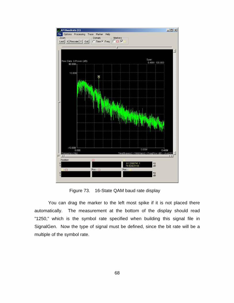
communication signals.
vi
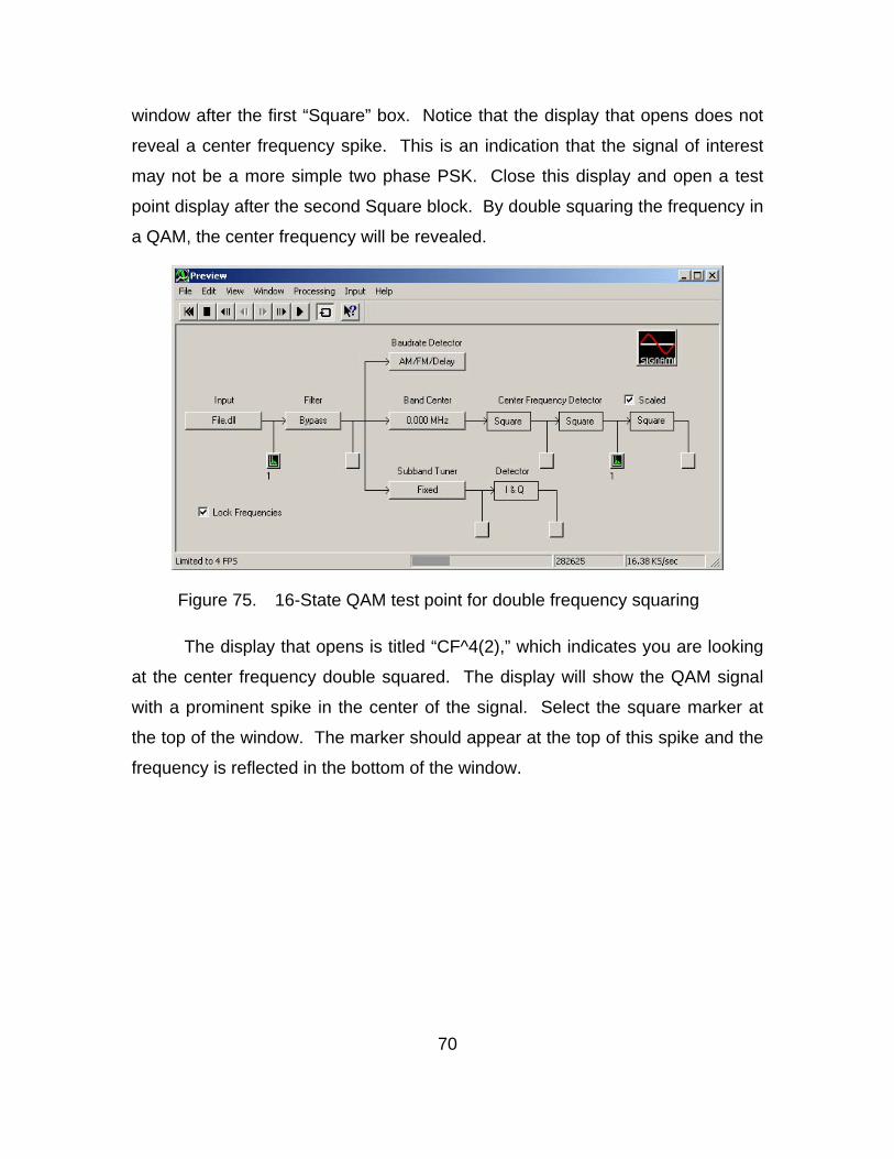
THIS PAGE INTENTIONALLY LEFT BLANK
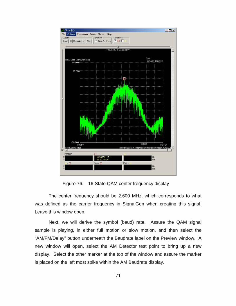
vii
TABLE OF CONTENTS
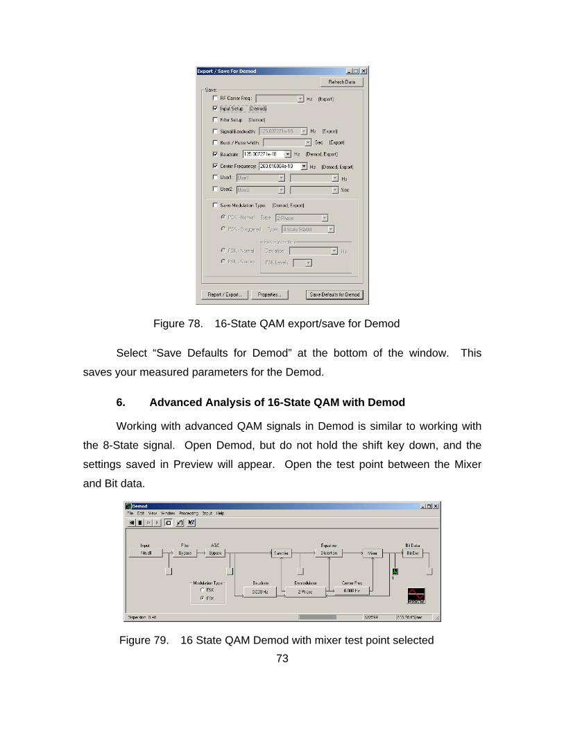
I. INTRODUCTION............................................................................................. 1 A. OVERVIEW OF SIGNALWORKS® SOFTWARE SUITE .................... 1 B. OBJECTIVE ......................................................................................... 2 C. THESIS ORGANIZATION.................................................................... 2
II. PHASE-SHIFT KEYED SIGNAL ANALYSIS ................................................. 5 A. OVERVIEW OF PHASE-SHIFT KEYED SIGNALS ............................. 5
1. Signal Characteristics ............................................................. 5 2. Applications ............................................................................. 6
B. GENERATING TEST SIGNAL WITH SIGNALGEN............................. 7 1. Procedural Guidance............................................................... 7 2. Creating a BPSK Signal using the Signalworks®
SignalGen Application ............................................................ 7 C. INITIAL ANALYSIS WITH PREVIEW ................................................ 15
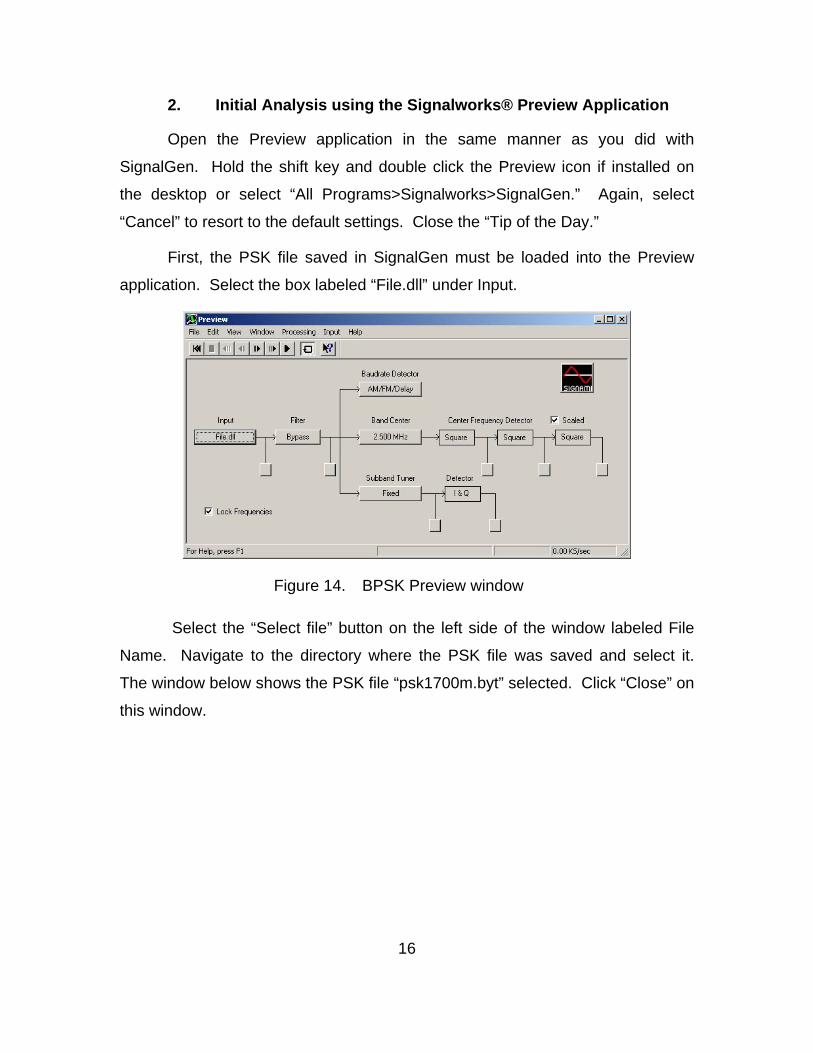
1. Procedural Guidance............................................................. 15 2. Initial Analysis using the Signalworks® Preview
Application ............................................................................. 16 D. ADDITIONAL ANALYSIS WITH DEMOD.......................................... 23
1. Procedural Guidance............................................................. 23 2. Advanced Analysis with Demod........................................... 23
E. BPSK ANALYSIS RESULTS............................................................. 24
III. QUADRATURE PHASE-SHIFT KEYED SIGNAL ANALYSIS ..................... 27 A. OVERVIEW OF QUADRATURE PHASE-SHIFT KEYED SIGNALS. 27
1. Signal Characteristics ........................................................... 27 2. Applications ........................................................................... 28
B. GENERATING QPSK TEST SIGNAL WITH SIGNALGEN ............... 28 1. Procedural Guidance............................................................. 28 2. Creating a QPSK Signal using the Signalworks®
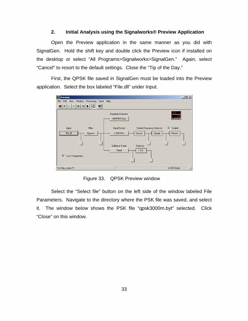
SignalGen Application .......................................................... 28 C. INITIAL ANALYSIS WITH PREVIEW ................................................ 32
1. Procedural Guidance............................................................. 32 2. Initial Analysis using the Signalworks® Preview
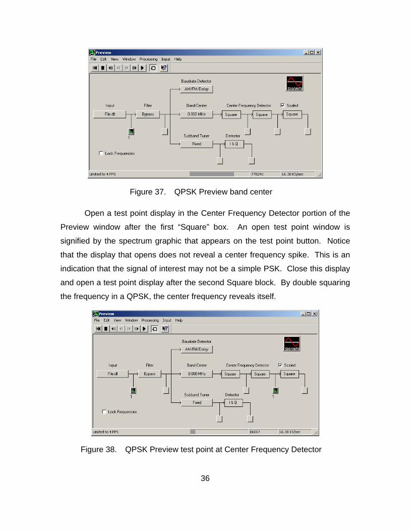
Application ............................................................................. 33 D. ADDITIONAL ANALYSIS WITH DEMOD.......................................... 40
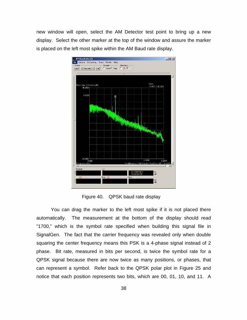
1. Procedural Guidance............................................................. 40 2. Advanced Analysis with Signalworks’® Demod
Application ............................................................................. 40 E. QPSK ANALYSIS RESULTS ............................................................ 43
IV. QUADRATURE AMPLITUDE MODULATION SIGNAL ANALYSIS ............ 45 A. OVERVIEW OF QUADRATURE AMPLITUDE MODULATION
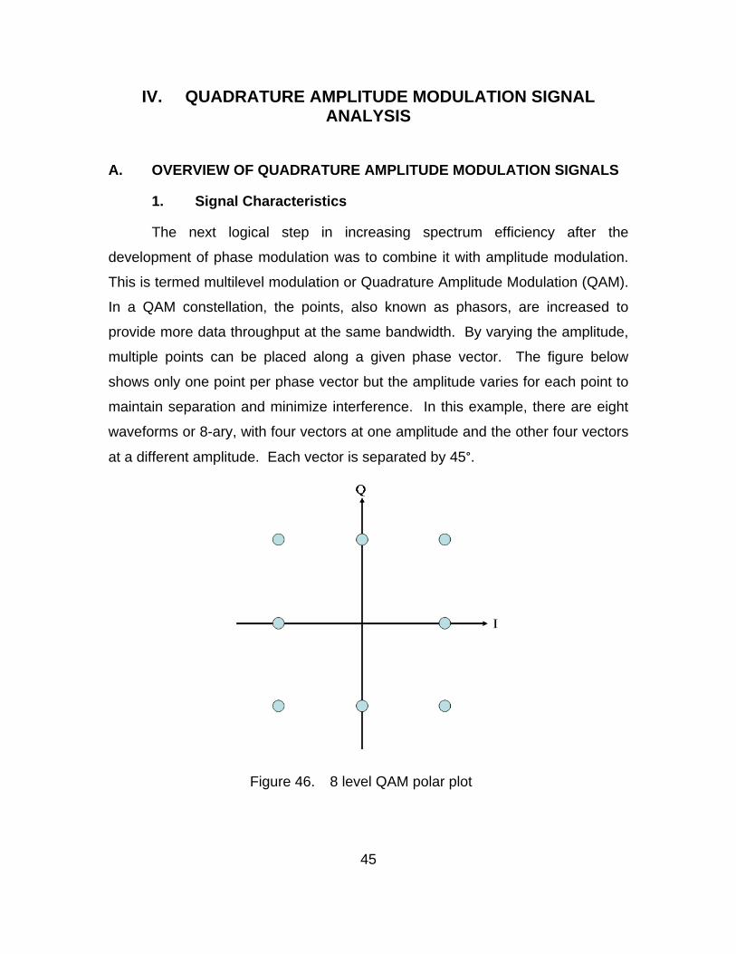
SIGNALS ........................................................................................... 45 1. Signal Characteristics ........................................................... 45
viii
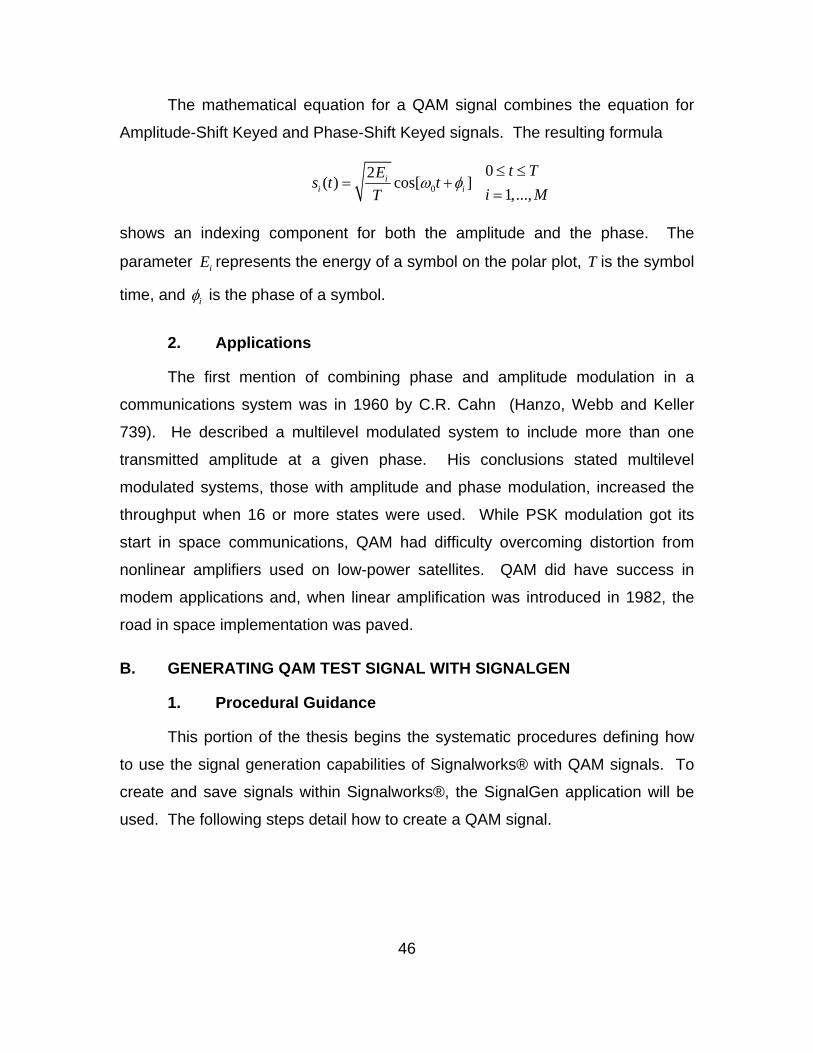
2. Applications ........................................................................... 46 B. GENERATING QAM TEST SIGNAL WITH SIGNALGEN ................. 46
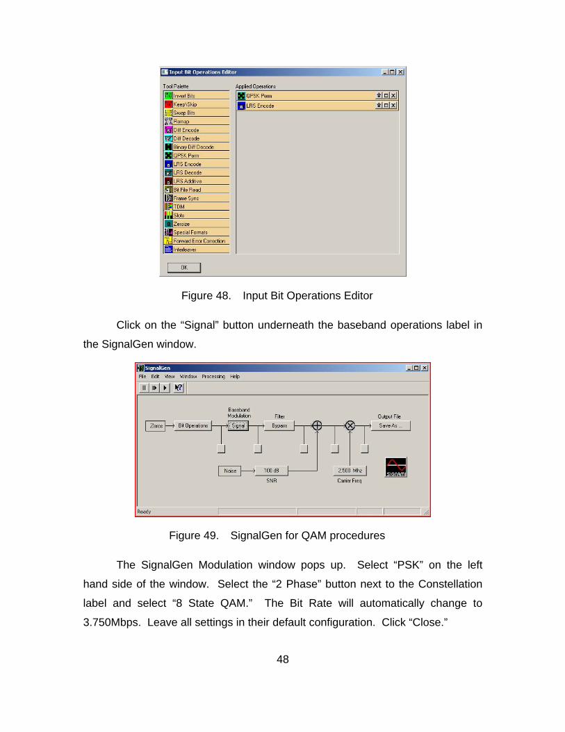
1. Procedural Guidance............................................................. 46 2. Creating a QAM Signal using the Signalworks®
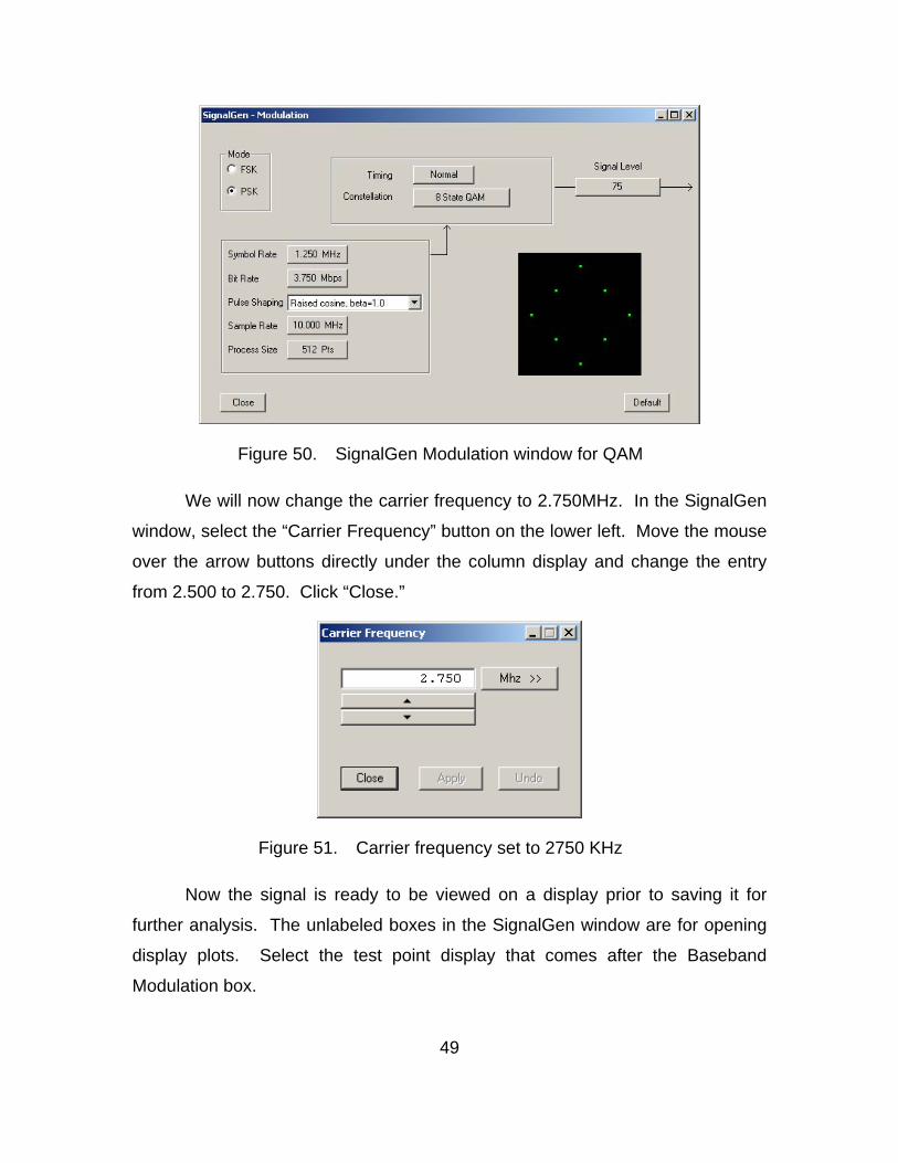
SignalGen Application .......................................................... 47 C. INITIAL QAM ANALYSIS WITH PREVIEW....................................... 51
1. Procedural Guidance............................................................. 51 2. Initial QAM Analysis using the Signalworks® Preview
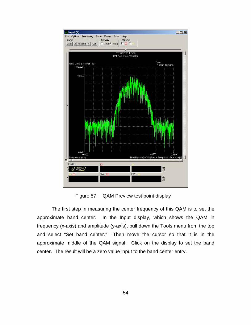
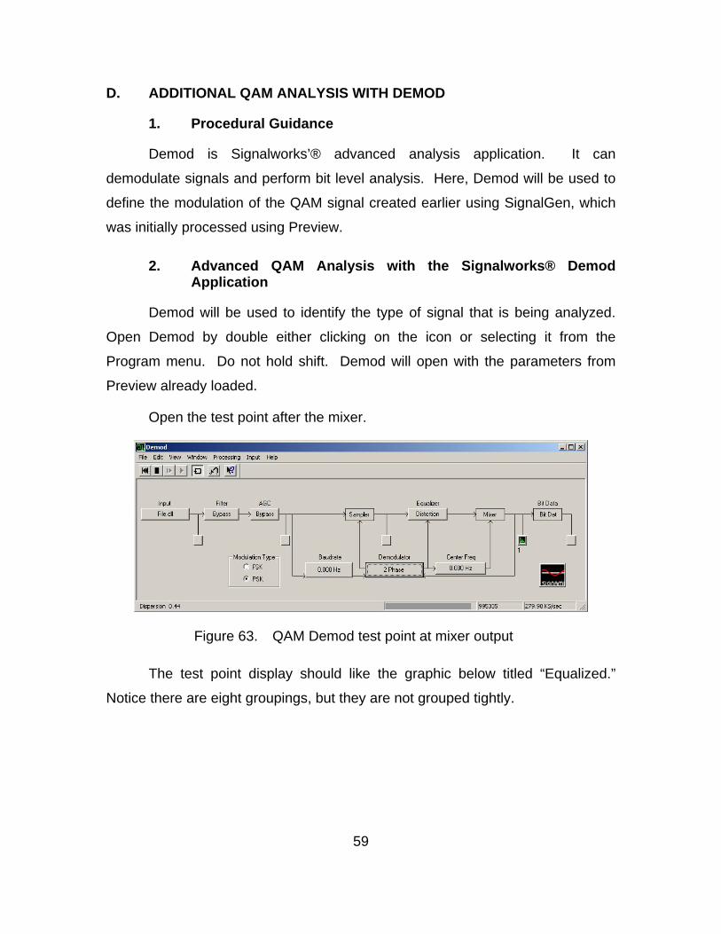
Application ............................................................................. 52 D. ADDITIONAL QAM ANALYSIS WITH DEMOD ................................ 59
1. Procedural Guidance............................................................. 59 2 Advanced QAM Analysis with the Signalworks® Demod
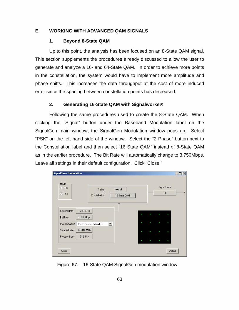
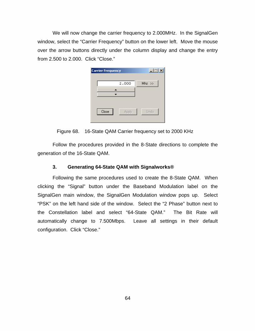
Application ............................................................................. 59 E. WORKING WITH ADVANCED QAM SIGNALS ................................ 63
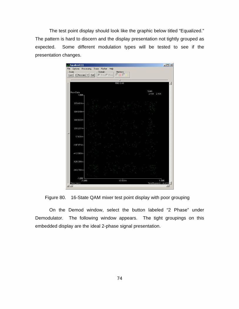
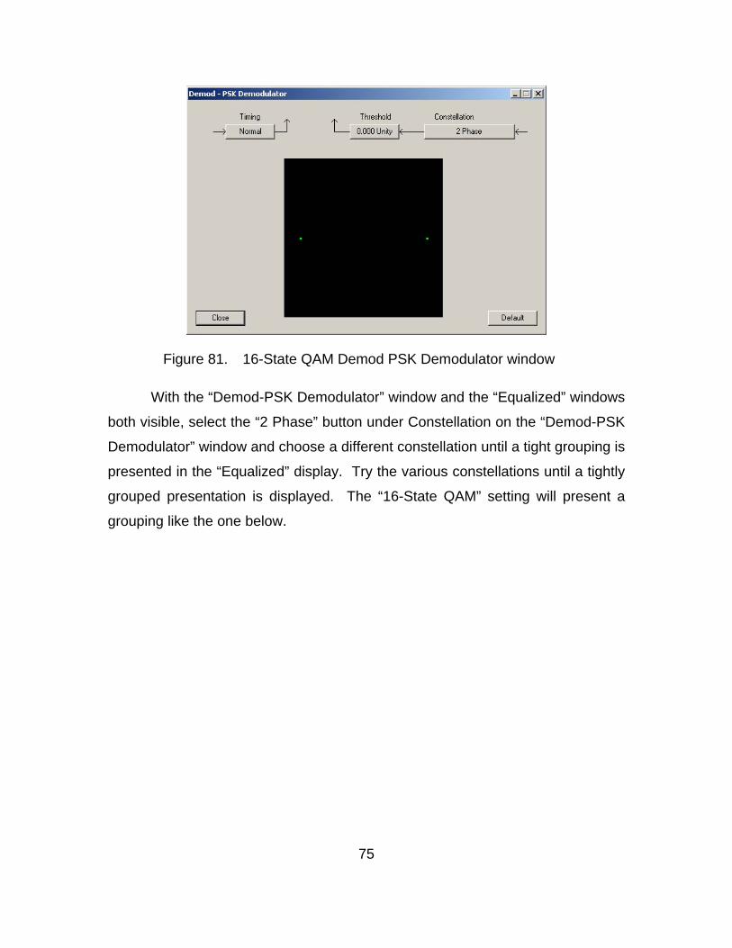
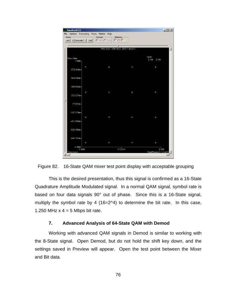
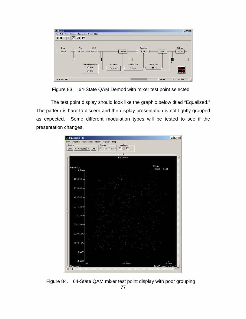
1. Beyond 8-State QAM ............................................................. 63 2. Generating 16-State QAM with Signalworks®..................... 63 3. Generating 64-State QAM with Signalworks®..................... 64 4. Initial analysis of 16-State QAM with Preview ..................... 65 5. Initial Analysis of 64-State QAM with Preview .................... 69 6. Advanced Analysis of 16-State QAM with Demod .............. 73 7. Advanced Analysis of 64-State QAM with Demod .............. 76
F. QAM ANALYSIS RESULTS .............................................................. 79
V. WI-FI SIGNAL ANALYSIS............................................................................ 81 A. OVERVIEW OF WIFI SIGNALS......................................................... 81
1. Signal Characteristics ........................................................... 81 2. Application ............................................................................. 81
B. INITIAL ANALYSIS WITH PREVIEW ................................................ 81 1. Procedural Guidance............................................................. 81 2. Initial Analysis using the Signalworks® Preview
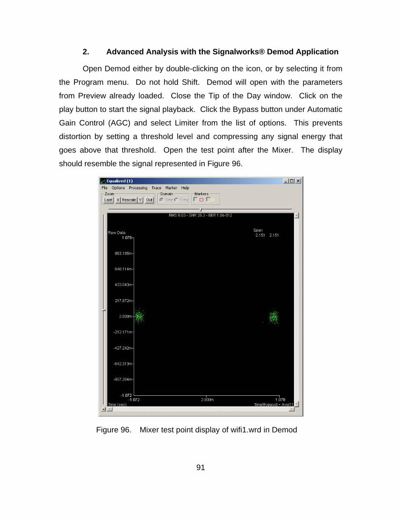
Application ............................................................................. 82 C. ADDITIONAL WIFI ANALYSIS WITH DEMOD ................................. 90
1. Procedural Guidance............................................................. 90 2. Advanced Analysis with the Signalworks® Demod
Application ............................................................................. 91 D. WIFI ANALYSIS RESULTS ............................................................. 100
VI. SUMMARY AND RECOMMENDATIONS FOR FUTURE WORK................ 101 A. SUMMARY....................................................................................... 101
1. Installation and Operation................................................... 101 2. Capabilities and Limitations ............................................... 102 3. Findings................................................................................ 102
B. RECOMMENDATIONS FOR FUTURE WORK................................ 103
LIST OF REFERENCES........................................................................................ 105
INITIAL DISTRIBUTION LIST ............................................................................... 107
ix
LIST OF FIGURES
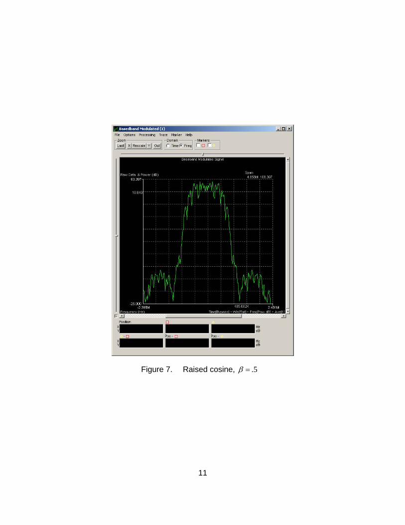
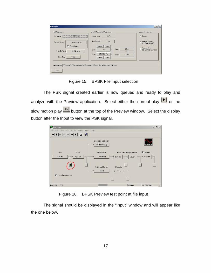
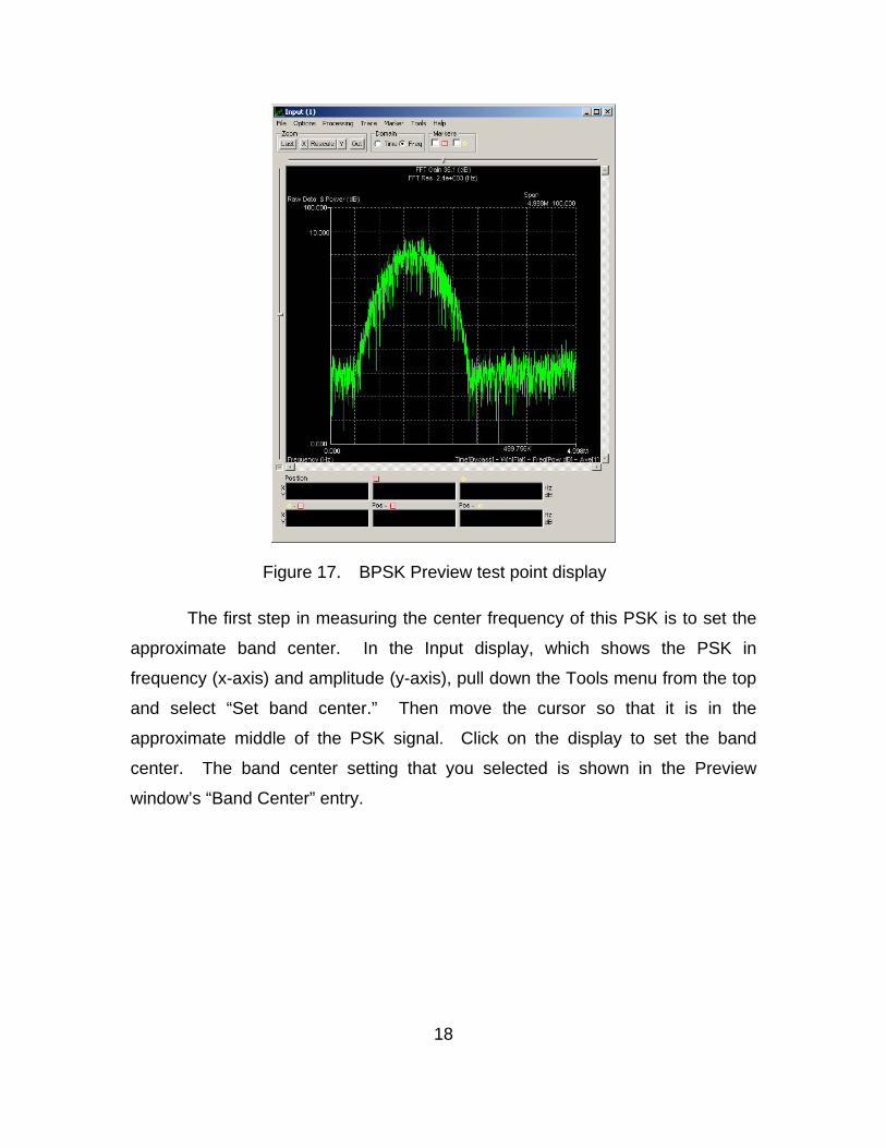
Figure 1. BPSK waveform ................................................................................... 5 Figure 2. BPSK polar plot .................................................................................... 6 Figure 3. Recall default parameters window........................................................ 7 Figure 4. Input bit operations editor ..................................................................... 8 Figure 5. SignalGen for BPSK procedures .......................................................... 8 Figure 6. Raised cosine, 0 (Nyquist minimum bandwidth) ........................... 10 Figure 7. Raised cosine, .5 ......................................................................... 11 Figure 8. Raised cosine, 1 ........................................................................... 12 Figure 9. SignalGen modulation window for BPSK............................................ 13 Figure 10. Carrier frequency default .................................................................... 13 Figure 11. Carrier frequency set to 1700 KHz ..................................................... 13 Figure 12. SignalGen test point at Baseband Modulation output......................... 14 Figure 13. BPSK Baseband Modulated test point display ................................... 15 Figure 14. BPSK Preview window ....................................................................... 16 Figure 15. BPSK File input selection ................................................................... 17 Figure 16. BPSK Preview test point at file input .................................................. 17 Figure 17. BPSK Preview test point display ........................................................ 18 Figure 18. BPSK Preview band center specified ................................................. 19 Figure 19. BPSK Preview test point at Center Freq. Detector ............................. 19 Figure 20. BPSK center frequency marker .......................................................... 20 Figure 21. BPSK baud rate display...................................................................... 21 Figure 22. BPSK export/save for Demod............................................................. 22 Figure 23. BPSK Demod test point at mixer output ............................................. 23 Figure 24. BPSK Demod test point display.......................................................... 24 Figure 25. QPSK polar plot.................................................................................. 27 Figure 26. QPSK Recall default parameters window........................................... 29 Figure 27. Input Bit Operations Editor ................................................................. 29 Figure 28. SignalGen for QPSK procedures........................................................ 30 Figure 29. SignalGen Modulation window for QPSK ........................................... 30 Figure 30. Carrier frequency set to 3000 KHz ..................................................... 31 Figure 31. SignalGen test point at Baseband Modulation output......................... 31 Figure 32. QPSK Baseband Modulation test point display .................................. 32 Figure 33. QPSK Preview window....................................................................... 33 Figure 34. QPSK file input selection .................................................................... 34 Figure 35. QPSK Preview test point at file input .................................................. 34 Figure 36. QPSK Preview test point display ........................................................ 35 Figure 37. QPSK Preview band center................................................................ 36 Figure 38. QPSK Preview test point at Center Frequency Detector .................... 36 Figure 39. QPSK center frequency marker.......................................................... 37 Figure 40. QPSK baud rate display ..................................................................... 38 Figure 41. QPSK export/save for Demod ............................................................ 39 Figure 42. QPSK Demod test point at mixer output............................................. 40
x
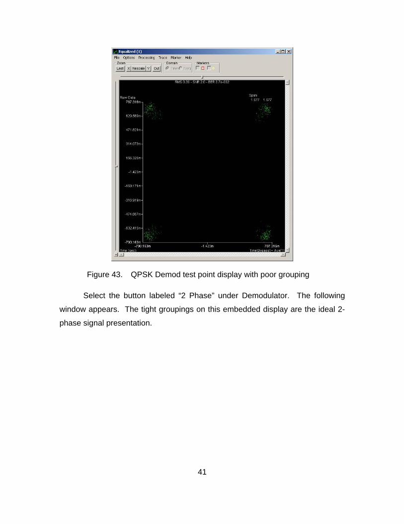
Figure 43. QPSK Demod test point display with poor grouping........................... 41 Figure 44. QPSK PSK demodulator .................................................................... 42 Figure 45. QPSK Demod test point display with optimal grouping....................... 43 Figure 46. 8 level QAM polar plot ........................................................................ 45 Figure 47. Recall default parameters window...................................................... 47 Figure 48. Input Bit Operations Editor ................................................................. 48 Figure 49. SignalGen for QAM procedures ......................................................... 48 Figure 50. SignalGen Modulation window for QAM............................................. 49 Figure 51. Carrier frequency set to 2750 KHz ..................................................... 49 Figure 52. SignalGen test point of Baseband Modulation output......................... 50 Figure 53. QAM Baseband Modulation test point display .................................... 51 Figure 54. QAM Preview window......................................................................... 52 Figure 55. QAM file input selection...................................................................... 53 Figure 56. QAM Preview test point at file input.................................................... 53 Figure 57. QAM Preview test point display.......................................................... 54 Figure 58. QAM Preview band center specification ............................................. 55 Figure 59. QAM Preview test point at Center Frequency Detector ...................... 55 Figure 60. QAM center frequency marker ........................................................... 56 Figure 61. QAM baud rate display ....................................................................... 57 Figure 62. QAM export/save for Demod .............................................................. 58 Figure 63. QAM Demod test point at mixer output............................................... 59 Figure 64. QAM Demod test point display with poor groupings ........................... 60 Figure 65. QAM Demod PSK Demodulator window ............................................ 61 Figure 66. QAM Demod test point display with acceptable groupings................. 62 Figure 67. 16-State QAM SignalGen modulation window.................................... 63 Figure 68. 16-State QAM Carrier frequency set to 2000 KHz.............................. 64 Figure 69. 64-State QAM SignalGen modulation window.................................... 65 Figure 70. 64-State QAM Carrier frequency set to 2,600 KHz............................. 65 Figure 71. 16-State QAM Preview test point for double squared center
frequency............................................................................................ 66 Figure 72. 16-State QAM test point display for double carrier frequency ............ 67 Figure 73. 16-State QAM baud rate display ........................................................ 68 Figure 74. 16-State QAM export/save for Demod window................................... 69 Figure 75. 16-State QAM test point for double frequency squaring ..................... 70 Figure 76. 16-State QAM center frequency display ............................................. 71 Figure 77. 16-State QAM baud rate display ........................................................ 72 Figure 78. 16-State QAM export/save for Demod................................................ 73 Figure 79. 16 State QAM Demod with mixer test point selected.......................... 73 Figure 80. 16-State QAM mixer test point display with poor grouping ................. 74 Figure 81. 16-State QAM Demod PSK Demodulator window.............................. 75 Figure 82. 16-State QAM mixer test point display with acceptable grouping....... 76 Figure 83. 64-State QAM Demod with mixer test point selected ......................... 77 Figure 84. 64-State QAM mixer test point display with poor grouping ................. 77 Figure 85. 64-State QAM Demod PSK Demodulator window.............................. 78 Figure 86. 64-State QAM mixer test point display with acceptable grouping....... 79
xi
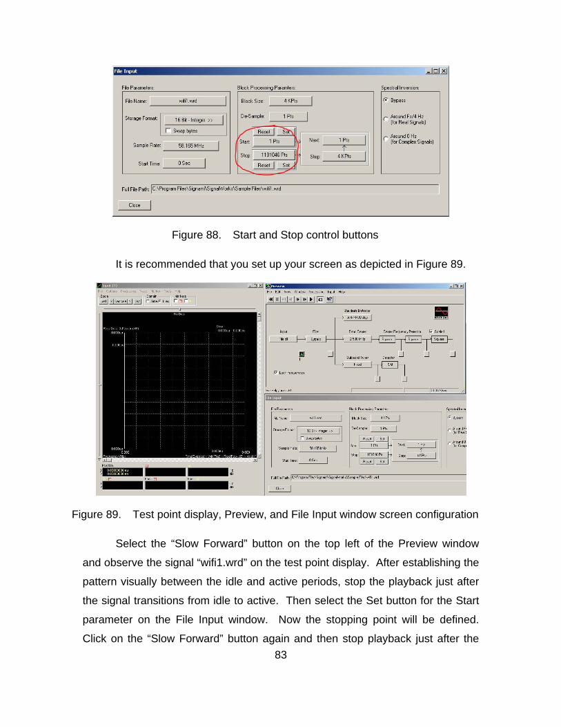
Figure 87. Recall window .................................................................................... 82 Figure 88. Start and Stop control buttons ............................................................ 83 Figure 89. Test point display, Preview, and File Input window screen
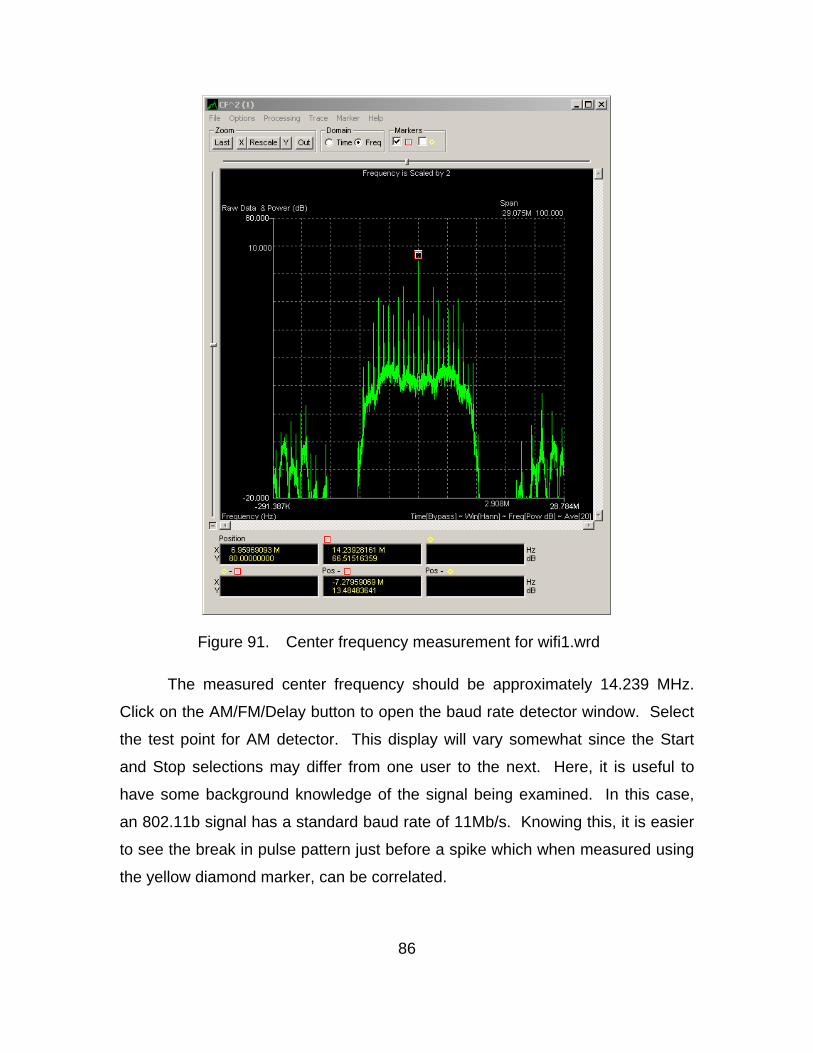
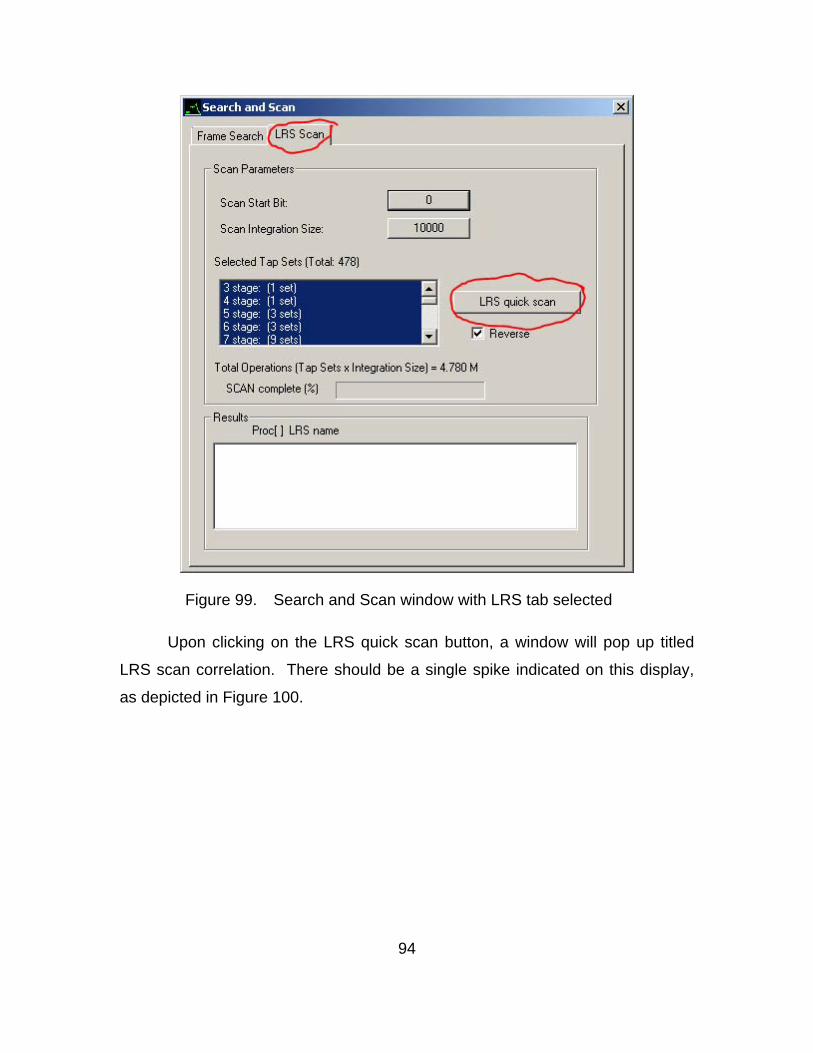
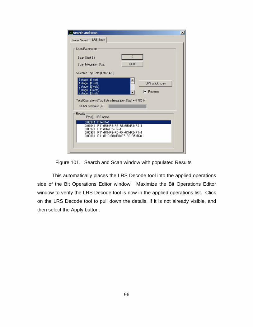
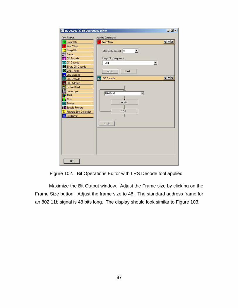
configuration....................................................................................... 83 Figure 90. Filter Setup for wifi1.wrd ..................................................................... 85 Figure 91. Center frequency measurement for wifi1.wrd ..................................... 86 Figure 92. Baudrate detector display with 11Mb/s wifi1.wrd signal...................... 87 Figure 93. Inaccurate center frequency depicted in I&Q test point display .......... 88 Figure 94. IQ display with adjusted frequency..................................................... 89 Figure 95. Export/Save for Demod window ......................................................... 90 Figure 96. Mixer test point display of wifi1.wrd in Demod.................................... 91 Figure 97. Bit Operations display for wifi1.wrd..................................................... 92 Figure 98. Bit Operations Editor with Keep/Skip tool with expanded functions.... 93 Figure 99. Search and Scan window with LRS tab selected ............................... 94 Figure 100. LRS Scan Correlation with single spike.............................................. 95 Figure 101. Search and Scan window with populated Results .............................. 96 Figure 102. Bit Operations Editor with LRS Decode tool applied........................... 97 Figure 103. Bit Output display with 48 bit frame size............................................. 98 Figure 104. Bit Output with 0-F Hex display .......................................................... 99 Figure 105. HEX display with highlighted MAC addresses.................................. 100
xii
THIS PAGE INTENTIONALLY LEFT BLANK
xiii
LIST OF ACRONYMS AND ABBREVIATIONS
AGC Automatic gain control
BPSK Binary Phase-Shift Keyed
EW Electronic Warfare
FSK Frequency Shift Keyed
GMSK Gaussian=Minimum Shift Keyed
LRS Linear Recursive Sequence
MB/s Megabits per second
MSK Minimum-Shift Keyed
OFDM Orthogonal Frequency Division Multiplexed
PSK Phase-Shift Keyed
QAM Quadrature Amplitude Modulation
QPSK Quadrature Phase-Shift Keyed
RF Radio Frequency
RFID Radio Frequency Identification
WLAN Wireless Local Area Network
WMAN Wireless Metropolitan Area Network
xiv
THIS PAGE INTENTIONALLY LEFT BLANK
xv
ACKNOWLEDGMENTS
I thank my wife, children, and extended family for enduring countless
hours of my absence while I was completing this project. They are the
foundation of my success in the Navy and are most deserving of recognition.
Their love and support through this and previous tours is the wind in my sails. I
also thank Professor Tri Ha for his determination and guidance as my advisor.
His background in signals and signal theory is extensive, and has proven critical
to my research. Additionally, I thank Professor Vicente Garcia, whom I sought
out as a fellow Cryptologist in search of research assistance. Although retired,
he is a staunch advocate for our community and continues to serve us well. The
staff at Signami-DCS were outstanding in their support. I specifically wish to
thank Mr. Terry Cutshaw, Mr. Jacob Rorick, and Mr. Gary Kenworthy for their
guidance and technical assistance.
xvi
THIS PAGE INTENTIONALLY LEFT BLANK
1
I. INTRODUCTION
A. OVERVIEW OF SIGNALWORKS® SOFTWARE SUITE
The Signalworks® software package developed by Signami-DCS is a
Windows or Linux based suite of software tools that incorporates complex
algorithms to enable advanced signals analysis. When coupled to a digital input,
Signalworks® offers all the advantages of typical analysis equipment such as
digital oscilloscopes, spectrum analyzers, and demodulators, combined into a
simple to use interface requiring no programming or coding. Input to
Signalworks® is accomplished via prerecorded files or through a digitizing
component directly input to the computer. Signalworks® is capable of
processing a variety of signal formats including Phase-Shift Keyed (PSK),