NAVAL POSTGRADUATE SCHOOL MONTEREY, CALIFORNIA THESIS Approved for public release; distribution is unlimited THE INFLUENCE OF WIND ON HF RADAR SURFACE CURRENT FORECASTS by Francisco Moisés Soares Calisto de Almeida December 2008 Thesis Advisor: Jeffrey Paduan Second Reader: Curtis Collins
Transcript
NAVAL
POSTGRADUATE SCHOOL
MONTEREY, CALIFORNIA
THESIS
Approved for public release; distribution is unlimited
THE INFLUENCE OF WIND ON HF RADAR SURFACE CURRENT FORECASTS
by
Francisco Moisés Soares Calisto de Almeida
December 2008
Thesis Advisor: Jeffrey Paduan Second Reader: Curtis Collins
THIS PAGE INTENTIONALLY LEFT BLANK
i
REPORT DOCUMENTATION PAGE Form Approved OMB No. 0704-0188 Public reporting burden for this collection of information is estimated to average 1 hour per response, including the time for reviewing instruction, searching existing data sources, gathering and maintaining the data needed, and completing and reviewing the collection of information. Send comments regarding this burden estimate or any other aspect of this collection of information, including suggestions for reducing this burden, to Washington headquarters Services, Directorate for Information Operations and Reports, 1215 Jefferson Davis Highway, Suite 1204, Arlington, VA 22202-4302, and to the Office of Management and Budget, Paperwork Reduction Project (0704-0188) Washington DC 20503. 1. AGENCY USE ONLY (Leave blank)
2. REPORT DATE December 2008
3. REPORT TYPE AND DATES COVERED Master’s Thesis
4. TITLE AND SUBTITLE The Influence of Wind on HF Surface Current Forecasts 6. AUTHOR(S) Francisco M. S. C. de Almeida
5. FUNDING NUMBERS
7. PERFORMING ORGANIZATION NAME(S) AND ADDRESS(ES) Naval Postgraduate School Monterey, CA 93943-5000
8. PERFORMING ORGANIZATION REPORT NUMBER
9. SPONSORING /MONITORING AGENCY NAME(S) AND ADDRESS(ES) N/A
10. SPONSORING/MONITORING AGENCY REPORT NUMBER
11. SUPPLEMENTARY NOTES The views expressed in this thesis are those of the author and do not reflect the official policy or position of the Department of Defense or the U.S. Government. 12a. DISTRIBUTION / AVAILABILITY STATEMENT Approved for public release; distribution is unlimited.
12b. DISTRIBUTION CODE
13. ABSTRACT (maximum 200 words) The ability to predict surface currents can have a beneficial impact in several activities such as Search and
Rescue and Oil Spill Response, as well as others more purely scientific, operational or economic. The Naval Postgraduate School, in conjunction with the Romberg Tiburon Center and the University of California Santa Barbara, has been studying this purpose for the Coastal Response Research Center, University of New Hampshire and NOAA. So far the prediction was based on tide and persistence of the reminiscent current. Faced with increasing error under changing environmental conditions, further study of other influences became fundamental, in order to increase reliability. This study is a part of that effort by studying the impact of wind-induced currents on forecasting.
Based on a year and a half of wind and HF surface current readings, the wind surface current interaction is analyzed and quantified. Then that influence is plugged into the forecast algorithm. The final results show that the wind driven surface current is about 2% of the wind magnitude rotating around 50º clockwise, with coherence after 17h. The wind introduction into the forecast improved the accuracy, but only by an average of 10%. The error still climbs with the variability of the environment, but knowing the wind influence allows other factors’ influences to be observed more accurately, such s the magnitude of the current itself. Forecasting is now done with 0.15 m/s plus or minus 0.1 m/s at 95% confidence.
UU NSN 7540-01-280-5500 Standard Form 298 (Rev. 2-89) Prescribed by ANSI Std. 239-18
ii
THIS PAGE INTENTIONALLY LEFT BLANK
iii
Approved for public release; distribution is unlimited
THE INFLUENCE OF WIND ON HF RADAR SURFACE CURRENT FORECASTS
Francisco M. S. C. de Almeida
Lieutenant Commander, Portuguese Navy B.S., Escola Naval (Portuguese Naval Academy), 1996
Submitted in partial fulfillment of the requirements for the degree of
MASTER OF SCIENCE IN PHYSICAL OCEANOGRAPHY
from the
NAVAL POSTGRADUATE SCHOOL December 2008
Author: Francisco Almeida
Approved by: Jeffrey Paduan Thesis Advisor
Curtis Collins Second Reader
Jeffrey Paduan Chairman, Department of Oceanography
iv
THIS PAGE INTENTIONALLY LEFT BLANK
v
ABSTRACT
The ability to predict surface currents can have a beneficial impact in several
activities, such as Search and Rescue and Oil Spill Response, as well as others more
purely scientific, operational or economic. The Naval Postgraduate School, in
conjunction with the Romberg Tiburon Center and the University of California Santa
Barbara, has been studying this purpose for the Coastal Response Research Center,
University of New Hampshire and NOAA. So far the prediction was based on tide and
persistence of the reminiscent current. Faced with increasing error under changing
environmental conditions, further study of other influences became fundamental, in order
to increase reliability. This study is a part of that effort by studying the impact of the
wind-induced currents on forecasting.
Based on a year and a half of wind and HF surface current readings, the wind
surface current interaction is analyzed and quantified. Then that influence is plugged into
the forecast algorithm. The final results show that the wind driven surface current is
about 2% of the wind magnitude rotating around 50º clockwise, with coherence after 17h.
The wind introduction into the forecast improved the accuracy, but only by an average of
10%. The error still climbs with the variability of the environment, but knowing the wind
influence allows other factors’ influences to be observed more accurately, such as the
magnitude of the current itself. Forecasting is now done with 0.15 m/s plus or minus 0.1
m/s at 95% confidence.
vi
THIS PAGE INTENTIONALLY LEFT BLANK
vii
TABLE OF CONTENTS
I. THE SURFACE CURRENTS FORECAST .............................................................1 A. APPLICATIONS .............................................................................................1
1. Navy Type Operations.........................................................................2 a. Special Operations ....................................................................2 b. Mine Warfare ............................................................................2 c. Flag Presence............................................................................3 d. Maneuvers and Evolutions .......................................................3 e. Weapons Practice......................................................................3
2. Coast Guard Type Operations............................................................3 a. Search and Rescue ....................................................................3 b. Oil Spill Response .....................................................................4 c. Illegal Traffic and Immigration ...............................................4 d. Patrol .........................................................................................4
3. Fisheries ................................................................................................4 a. For Those Who Monitor ...........................................................4 b. For the Fisherman....................................................................5
4. Meteorological/Oceanographic...........................................................5 5. Commercial and Recreational Navy ..................................................5 6. Habitat Impact .....................................................................................5
B. ACTUAL MODELS ........................................................................................5 1. The Naval Postgraduate School Model ..............................................6 2. The Coast Guard / University of Connecticut Model .......................7
C. FORECAST AND THE INTRODUCTION OF WIND INFLUENCE ......8
II. THE WIND / SURFACE CURRENT INTERACTION ..........................................9 A. PREVIOUS WORKS USED IN THIS STUDY ............................................9
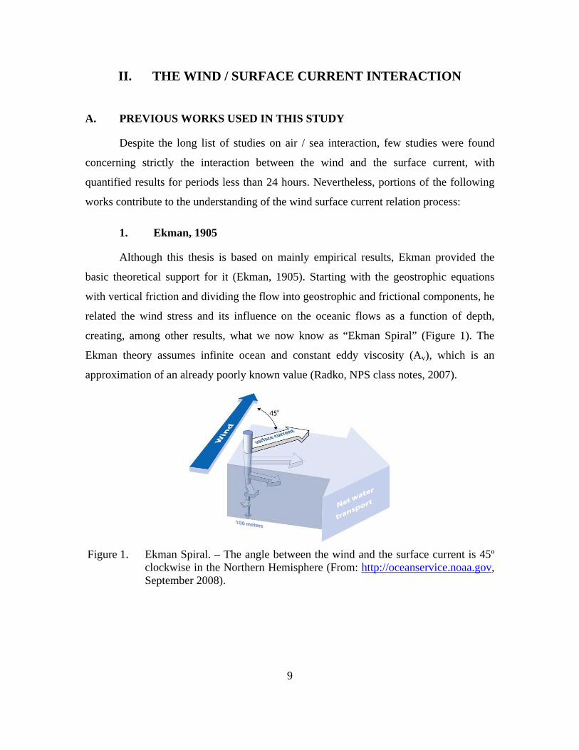
1. Ekman, 1905 .........................................................................................9 2. McNally, Luther and White, 1988....................................................10
a. The angle .................................................................................11 b. Correlation ..............................................................................11 c. Major Axis ...............................................................................11 d. Lags..........................................................................................11
3. Foster, 1993.........................................................................................11 4. Xu and Bowen, 1993; Monismith et al., 2006 ..................................12 5. Yelland and Taylor, 1995 ..................................................................12 6. Ardhuin, Chapron and Elfouhaily, 2003 .........................................12 7. Ullman et al., 2003..............................................................................12 8. O’Donnall et al., 2005 ........................................................................13 9. Garfield, Paduan and Ohlmann, 2007 .............................................13 10. Ardhuin et al., October 2008.............................................................13
B. DATA ..............................................................................................................14 1. Winds ..................................................................................................15
a. NDBC Buoys ...........................................................................16
viii
b. MBARI Buoys .........................................................................17 c. Resolution and Accuracy ........................................................17 d. Handling..................................................................................18 e. Other Series Created ...............................................................18
2. Currents ..............................................................................................18 a. CODAR Technology ...............................................................19 b. CODAR Stations .....................................................................21 c. Resolution and Accuracy ........................................................23 d. Handling..................................................................................23 e. Other Series Created ...............................................................23
3. Both Wind and Current ....................................................................24 C. EMPIRICAL APPROACH...........................................................................24
1. Principal Axis (Biggest Variance).....................................................24 2. Complex Correlation (Kundu, 1975)................................................26 3. Scatter Comparison ...........................................................................28 4. Auto Correlation (McMahan and Wyland, NPS Lab Software,
2007) ....................................................................................................31 5. Power Spectra and Straight Coherence...........................................35 6. Rotary Spectra (Gonnela, 1972 and Mooers, 1972, Bahr, 2007
Software).............................................................................................37 7. Vector Cross Spectral Analysis (Mooers, 1972 and McNally et
al, 1989, After Jessen and Bahr, 2007 software) .............................40 D. THEORETICAL APPROACH ....................................................................42 E. COMPARISON..............................................................................................43 F. CONCLUSIONS ............................................................................................43
1. Transfer Function ..............................................................................44 a. Magnitude................................................................................44 b. Angle........................................................................................44
III. THE FORECAST ......................................................................................................45 A. FORECAST WITH CODAR........................................................................45
1. Reliability of a Forecast.....................................................................45 2. Accuracy of a Forecast ......................................................................45
B. PREVIOUS ATTEMPTS..............................................................................46 1. Problems .............................................................................................46 2. Results .................................................................................................46
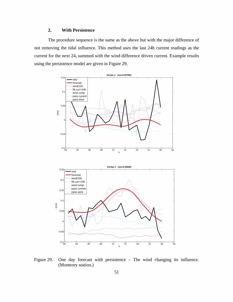
C. THE INTRODUCTION OF WIND .............................................................47 1. With Tides Treatment .......................................................................48 2. With Persistence.................................................................................51
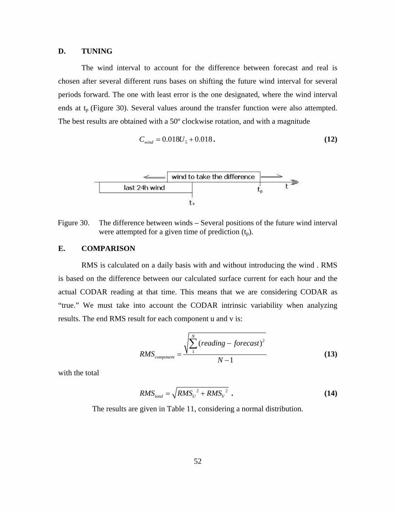
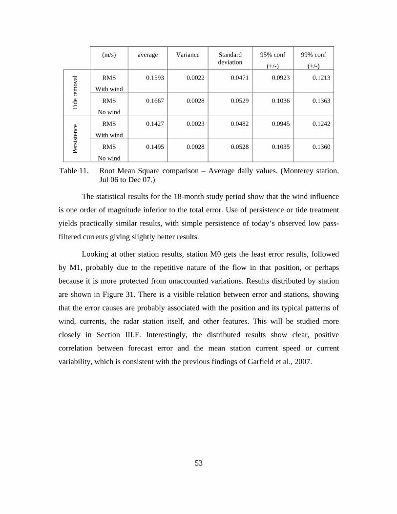
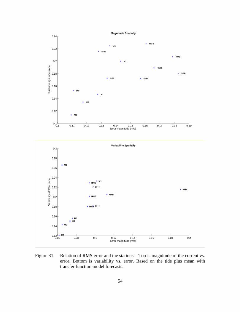
D. TUNING..........................................................................................................52 E. COMPARISON..............................................................................................52 F. ERROR CAUSES ..........................................................................................57
1. Accuracy Expectancy.........................................................................58 a. CODAR (From Wright, 2008) ................................................58 b. Winds .......................................................................................58
ix
c. Tides (Pawlowicz et al., 2002).................................................58 d. Growing Surface Waves (Ardhuin et al., 2003).....................58 e. Eddy Surface Velocity.............................................................58 f. Others ......................................................................................58
IV. CONCLUSIONS ........................................................................................................63 A. THE WIND INFLUENCE ............................................................................63 B. RESULT CAPABILITIES............................................................................64 C. NEXT STEPS .................................................................................................64
LIST OF REFERENCES......................................................................................................67
INITIAL DISTRIBUTION LIST .........................................................................................71
x
THIS PAGE INTENTIONALLY LEFT BLANK
xi
LIST OF FIGURES
Figure 1. Ekman Spiral. – The angle between the wind and the surface current is 45º clockwise in the Northern Hemisphere (From: http://oceanservice.noaa.gov, September 2008). ...............................................9
Figure 2. Matching data of Wind and Current – Each jump in the line corresponds to an interval with no data....................................................................................14
Figure 3. Current and Wind reading stations – Dots represent one example hourly coverage of the Pescadero CODAR station. (From: ArcGIS. Coastline from NOAA, National Ocean Service, 1994.) .................................................15
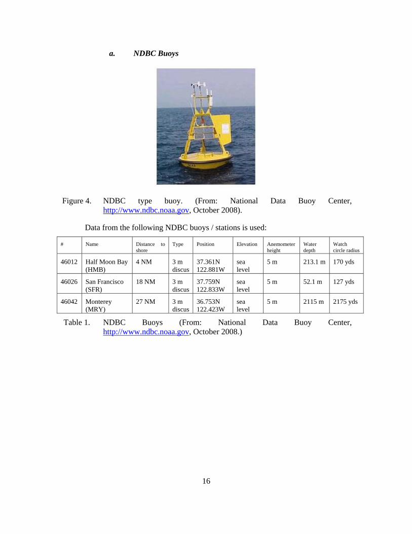
Figure 4. NDBC type buoy. (From: National Data Buoy Center, http://www.ndbc.noaa.gov, October 2008)......................................................16
Figure 5. MBARI M0 and M1 buoys. (From: http://www.mbari.org, October 2008)...17 Figure 6. Point Sur CODAR station – The receiver antenna is closer and the
transmitter further down. (From: CODAR, http://www.codaros.com, October 2008). .................................................................................................19
Figure 7. Bragg scattering phenomenon – The biggest return in scattered energy is ½ λ (wavelength) of the sea wave. (From: Martin, 2004 in “An introduction to Ocean Remote Sensing,” Cambridge.)....................................20
Figure 8. Bragg scattering phenomenon. Received power by frequency – The difference of where the peak is and where it should be for that particular λ , is proportional to the radial current velocity. (From: Paduan & Graber, 1997.) ...............................................................................................................21
Figure 9. Principal axis analysis – Values correspond to variance and alfa is the angle between the two full lines. (Monterey station.)......................................25
Figure 10. Complex correlation – Modulus is a measure of correlation and alpha is the physical angle. (Monterey station.)............................................................27
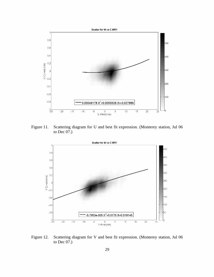
Figure 11. Scattering diagram for U and best fit expression. (Monterey station, Jul 06 to Dec 07.)........................................................................................................29
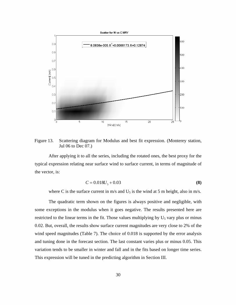
Figure 12. Scattering diagram for V and best fit expression. (Monterey station, Jul 06 to Dec 07.)........................................................................................................29
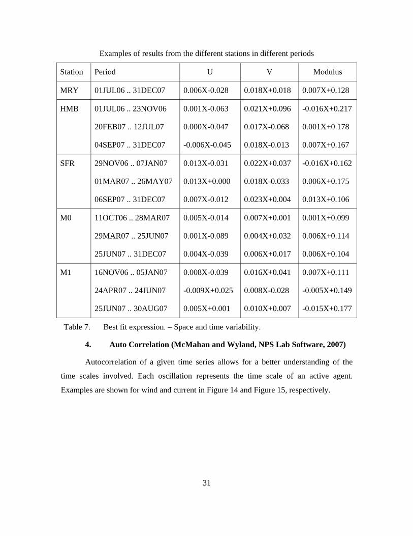
Figure 13. Scattering diagram for Modulus and best fit expression. (Monterey station, Jul 06 to Dec 07.) .............................................................................................30
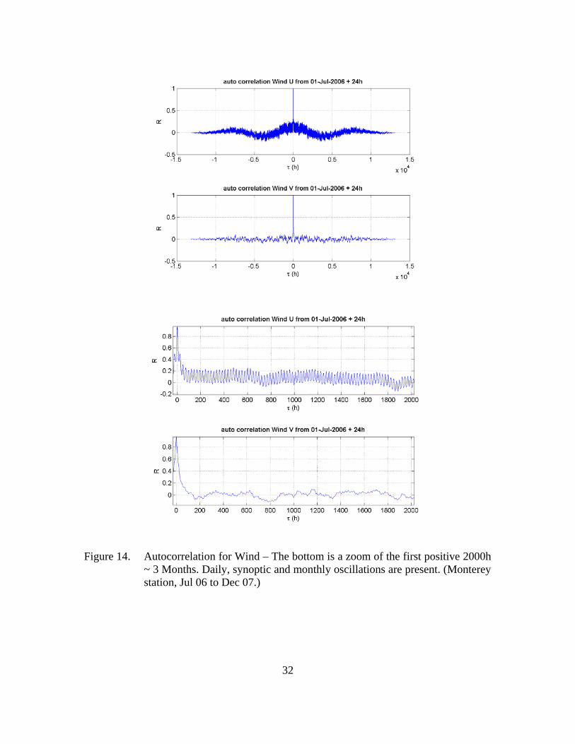
Figure 14. Autocorrelation for Wind – The bottom is a zoom of the first positive 2000h ~ 3 Months. Daily, synoptic and monthly oscillations are present. (Monterey station, Jul 06 to Dec 07.) ..............................................................32
Figure 15. Autocorrelation for Current – The bottom is a zoom of the first positive 2000h ~ 3 Months. Daily, synoptic and monthly oscillations are present. (Monterey station, Jul 06 to Dec 07.) ..............................................................33
Figure 16. Autocorrelation for Current with tides removed – The bottom is a zoom of the first positive 2000h ~ 3 Months. Daily, synoptic and monthly oscillations are present. (Monterey station, Jul 06 to Dec 07.)........................34
Figure 17. Power spectra of Wind and Current – Dashed at 95% confidence. (Monterey station, Jul 06 to Dec 07.) ..............................................................35
xii
Figure 18. Power spectra of Wind and Current with tides removed – Dashed at 95% confidence (Monterey station, Jul 06 to Dec 07.)............................................36
Figure 19. Coherence and Phase between wind and current – Dashed at 95% confidence. (Monterey station, Jul 06 to Dec 07.)...........................................37
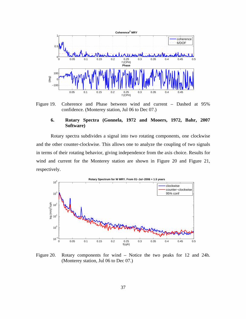
Figure 20. Rotary components for wind – Notice the two peaks for 12 and 24h. (Monterey station, Jul 06 to Dec 07.) ..............................................................37
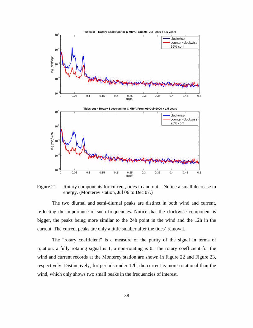
Figure 21. Rotary components for current, tides in and out – Notice a small decrease in energy. (Monterey station, Jul 06 to Dec 07.) .............................................38
Figure 22. Rotary coefficient for Wind – A fully rotational movement would be valued 1. (Monterey station, Jul 06 to Dec 07.)...............................................39
Figure 23. Rotary coefficient for Current, tides in and out. (Monterey station, Jul 06 to Dec 07.)........................................................................................................39
Figure 24. Complex Coherence and Phase – Lower image is a zoom of the coherent part. (Monterey station, Jul 06 to Dec 07.) ......................................................40
Figure 25. Complex coherence and Phase, tide removed – Top, all constituents. Bottom, all constituents removed but S1. (Monterey station, Jul 06 to Dec 07.) ...................................................................................................................42
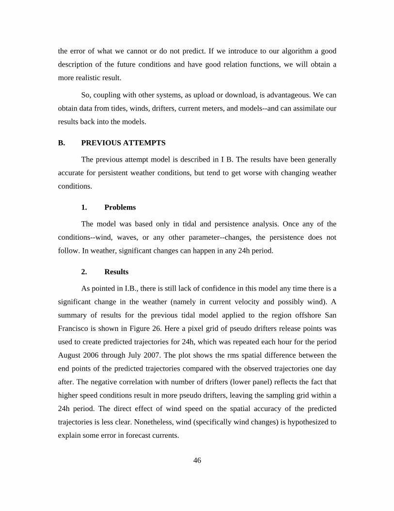
Figure 26. Results for RMS compared with wind and number of pseudo drifters – RMS for 24h. The number of pseudo drifters present may be used as a proxy for current speed. (Image from Garfield et al., 2007.)...........................47
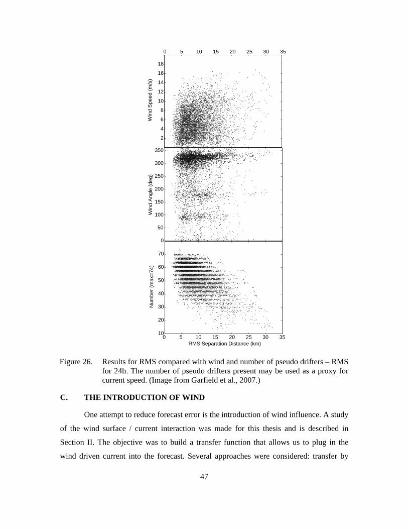
Figure 27. Basic flow chart diagram of the forecast procedure – Several adaptations were attempted. ................................................................................................48
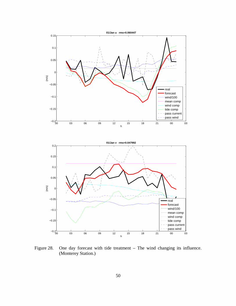
Figure 28. One day forecast with tide treatment – The wind changing its influence. (Monterey Station.) ..........................................................................................50
Figure 29. One day forecast with persistence – The wind changing its influence. (Monterey station.)...........................................................................................51
Figure 30. The difference between winds – Several positions of the future wind interval were attempted for a given time of prediction (tp)..............................52
Figure 31. Relation of RMS error and the stations – Top is magnitude of the current vs. error. Bottom is variability vs. error. Based on the tide plus mean with transfer function model forecasts.....................................................................54
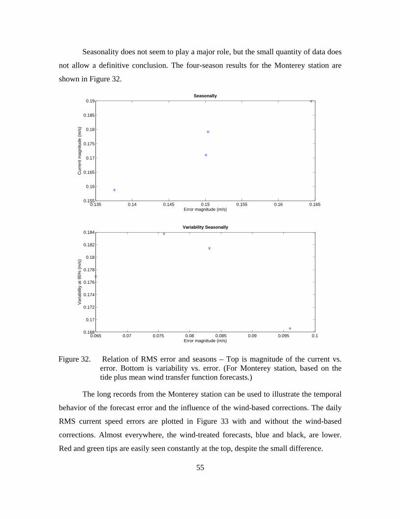
Figure 32. Relation of RMS error and seasons – Top is magnitude of the current vs. error. Bottom is variability vs. error. (For Monterey station, based on the tide plus mean wind transfer function forecasts.) ............................................55
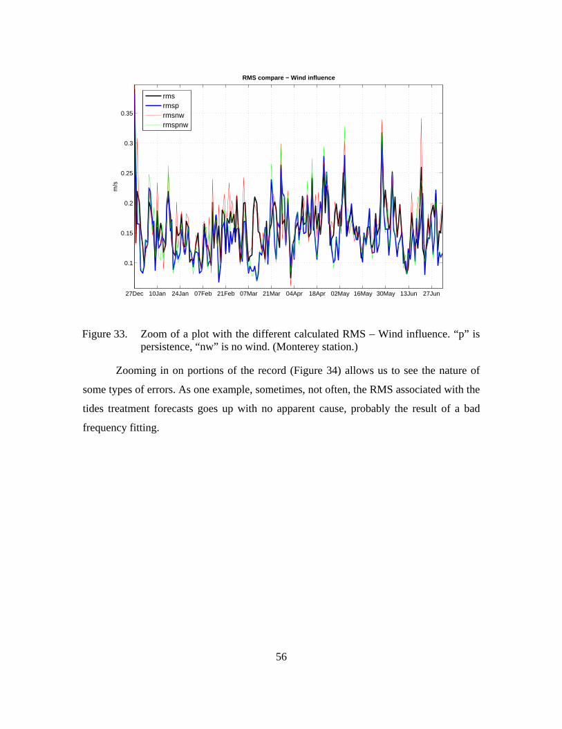
Figure 33. Zoom of a plot with the different calculated RMS – Wind influence. “p” is persistence, “nw” is no wind. (Monterey station.)...........................................56
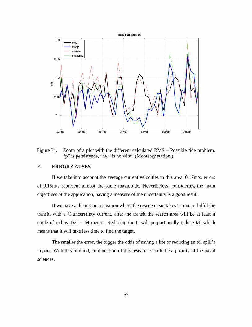
Figure 34. Zoom of a plot with the different calculated RMS – Possible tide problem. “p” is persistence, “nw” is no wind. (Monterey station.).................................57
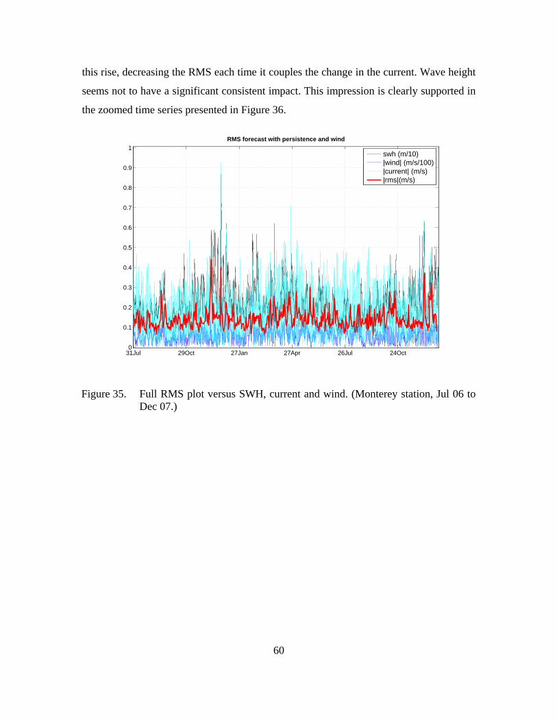
Figure 35. Full RMS plot versus SWH, current and wind. (Monterey station, Jul 06 to Dec 07.)............................................................................................................60
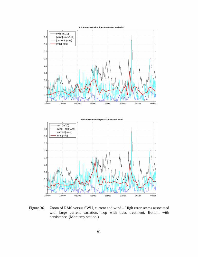
Figure 36. Zoom of RMS versus SWH, current and wind – High error seems associated with large current variation. Top with tides treatment. Bottom with persistence. (Monterey station.)...............................................................61
xiii
LIST OF TABLES
Table 1. NDBC Buoys (From: National Data Buoy Center, http://www.ndbc.noaa.gov, October 2008.).....................................................16
Table 2. MBARI Buoys (From: Monterey Bay Aquarium Research Institute, http://www.mbari.org, October 2008; Depths (From: ICON, http://www.oc.nps.edu/~icon/moorings, November 2008)..............................17
Table 3. CODAR stations (From: http://www.cencalcurrents.com, September 2008.) ...............................................................................................................22
Table 4. Principal axis analysis. – Values correspond to magnitudes and angle between the major axis and north. (Monterey station.) ...................................25
Table 5. Principal axis analysis. – Space and time variability (wind – current.) ...........26 Table 6. Complex correlation. – Space and time variability..........................................28 Table 7. Best fit expression. – Space and time variability.............................................31 Table 8. Added variances ~ energy. (Monterey station.)...............................................36 Table 9. Wind and Current shifting of angles in time. (Averages for all the stations
and periods.).....................................................................................................41 Table 10. Detidal errors with 3 days and 1 Month data – The calculation of the Root
Mean Square error will be discussed in III. E. (Monterey Station.) ................49 Table 11. Root Mean Square comparison – Average daily values. (Monterey station,
Jul 06 to Dec 07.) .............................................................................................53
xiv
THIS PAGE INTENTIONALLY LEFT BLANK
xv
LIST OF ACRONYMS
CODAR Coastal Ocean Dynamics Application Radar
EMR Electromagnetic Radiation
GDOP Geometric Dilution of Precision
MBARI Monterey Bay Aquarium Research Institute
NDBC National Data Buoy Center
NOAA National Oceanic and Atmospheric Administration
NPS Naval Postgraduate School
RMS Root Mean Square
SAR Search And Rescue
SAROPS SAR Optimal Planning System
SST Sea Surface Temperature
STPS Short Term Prediction System
SWH Significant Wave Height
xvi
THIS PAGE INTENTIONALLY LEFT BLANK
xvii
ACKNOWLEDGMENTS
The author would like to acknowledge the support of NOAA/UNH’s Coastal
Response Research Center at the University of New Hampshire.
The author would also like to express his gratitude and appreciation especially to
Professor Jeffrey Paduan and Oceanographers Mike Cook and Fred Bahr, who patiently
guided and facilitated all the work, and Professor Curt Collins who was so kind to be the
second reader. I would also like to thank the Oceanography Department faculty of NPS,
who encouraged the work and added so much to my understanding:
Professors Mary Batteen Peter Chu Ching-Sang Chiu Thomas Herbers Associate Professor Timour Radko Assistant Professor Jamie MacMahan Senior Lecturer Arlene Guest Research Associate John Joseph Oceanographers Chenwu Fan Paul Jessen Terry Rago Superv. Gen. Eng. Robert Wyland
I also appreciate the Oceanography and Meteorology/Oceanography students
from 2007/08, with whom so many questions were debated.
Finally, my wonderful wife, Cidália, is the Muse that always pushes me further
and further ahead.
xviii
THIS PAGE INTENTIONALLY LEFT BLANK
1
I. THE SURFACE CURRENTS FORECAST
A. APPLICATIONS
The use of the sea is not natural to man. Instead of moving with a solid surface
underneath his feet and an almost intangible fluid surrounding him, at sea he has to deal
with a much more viscous fluid. One of the major differences that this produces is that on
earth, if he stops moving his body, or his car, he stops. At sea, he doe not. In order to take
the best advantage of this distinction, understanding how this movement works is
necessary. In the fifteenth and sixteenth centuries, the Portuguese voyages of discovery
that navigated the entire globe in simple sailing ships relayed much of this knowledge.
Charts of currents were drawn and pilots were written in each trip.
With the passage of four centuries, several approaches have evolved to face the
challenges of today. One of them is the remote evaluation of the surface current by HF
RADAR (explained more in detail on II.B.2.a.). This method is excellent in filling the
gap between satellite remote sensing measurements and the shore; however, it is not good
for the Surf zone, for which other methods can be applied, like the one described in Puleo
et al., 2002. Depending on the frequency, HF radar can be used to read from around 3 to
200 km off the coast. Surface currents are obtained with regular readings through this
means, allowing the creation of a real time surface picture. Several works are still
debating the accuracy of this system and what influences it. This study, focused on the
forecast of the next 24 hours (24h) surface currents, takes the next logical step. Extracting
currents using electromagnetic radiation (EMR) on the HF band implies that all the
readings made are of the first two meters (2m) of depth, because EMR does not reach any
further down and in this shallow layer, wind is considered to be a major driver of the
currents.
There are not many studies considering the interaction between the previously
mentioned surface layer currents and wind, being almost all based on short time series
and with limited resolution, most under the inertial period (24h). The existence of a
database of two time series of both wind and current, with lengths over one year and with
2
an hourly resolution, presents an opportunity to unveil some properties of that interaction
that are currently poorly known. Based on these time series data (described in II.B.), this
thesis’s aim is to first find the surface current component that is driven by the wind, by
constructing a transfer function between them (described in Section II). This transfer
function will then be used as an extra input for an already existing forecast model that
relies solely on persistence and tides (described in I.B.), expecting to bring better
accuracy and reliability to it. The results obtained for the wind/surface current interaction
in this long time series may also be applied to many other future studies.
Due to its practical implications, several institutions are interested in systems that
allow this knowledge of the surface currents and in its forecast, because it has direct
impact to every sea user that needs to plan any type of short term deployment. That is the
case of the National Oceanic and Atmospheric Administration (NOAA) Coastal
Response Research Center, who funded a study on “Delivery and Quality Assurance of
Short-Term Trajectory Forecasts from HF Radar Observations,” of which this thesis is
also a part. Better knowledge of the next 24h surface currents may be used to get better
results in:
1. Navy Type Operations
Surface current forecasting has a significant impact on non-motorized activities,
because propulsion reduces the dependency on the flow to which the user is exposed.
a. Special Operations
Deployment of divers or any type of raft maneuvering at the coast may
benefit from a shortened mission time and energy, reducing risks and costs.
b. Mine Warfare
Locating the positions of drifting mines remains a modern reality because
mines are still the cheapest and most effective way of making constraints to the use of a
certain sea area or a harbor. To avoid or to sweep drifting mines, knowing where a field
3
is today will not help much tomorrow, because the mines drift with the current at their
depth. If you are deploying, you need to know if the mine behavior will be what you
intend.
c. Flag Presence
Most flag presence missions consist of long periods where a ship is
constrained to a certain position or box. Taking advantage of the currents will result in
better efficiency in the use of time and fuel.
d. Maneuvers and Evolutions
To maneuver a ship a long distance, the vector of her self propelled
velocity must be added to the surface current velocity, also resulting in better efficiency
in the use of time and fuel.
e. Weapons Practice
Target drift in time.
In live surface fire practice, usually a target is deployed or towed at a very
slow speed. More accurate knowledge of the current will predict target drift over time,
allowing a better residence time in the exercise area with fewer maneuvers, making it
safer.
2. Coast Guard Type Operations
a. Search and Rescue
Most distressed platforms do not have, or only have partial, locomotion
capability. Examples are man overboard, life saving rafts, debris or a damaged ship.
Having the correct surface current scenario will allow two major advantages:
(1) Reduces Position Uncertainty to the Distressed Position.
The future target position is a function of time multiplied by the elements’ influence.
When the rescue craft reaches the search zone, it usually has to face an area which size
depends on the uncertainty of the surface current and the wind influence on the target
4
(and the initial position error). Reducing surface current uncertainty will directly reduce
the search area, reducing the time needed to find the target, allowing better survivability
odds.
(2) Rescue Missions Savings in Hours and Fuel. Added to the
advantage in (1) of facing a shorter area, rescuers are able to plan a more accurate
intercept course, arriving earlier than possible previously which results in an even tighter
search area. On the scene, better sweeping plans can be made.
b. Oil Spill Response
Knowledge of the impact area, where a spill occurred and where it is
going, allows the efficient deployment of the available means, reducing damage. For a
good result, it must be coupled with the pollutant’s dispersive characteristics. Also, it
helps track pollutants that may have come from tank washings.
c. Illegal Traffic and Immigration
Much of this traffic is done by small slow boats, for which the surface
current is a determinant of the true course. Also, sometimes packages are sent adrift on
purpose or to avoid capture. Knowing the currents will facilitate the collection of them.
d. Patrol
Better efficiency in the use of time, fuel and area covered.
3. Fisheries
a. For Those Who Monitor
One typical periodic problem is the understanding of how a bloom will
spread out. Knowing more about buoyant behaviors helps avoid the capture and
consumption of organisms that may have toxic elements. Also, surface current
knowledge gives a better understanding of the probable paths of buoyant (or slow
velocity) organisms, such as eggs, larvae or youngsters.
5
b. For the Fisherman
Coastal fishermen depend a lot on timing and their profits depend a lot on
fuel consumption. The knowledge of how the currents will behave provides a tool to
make transits and staying with fisheries’ spots more cost efficient. They also benefit from
more accurate knowledge of the species behavior described in the previous paragraph.
4. Meteorological/Oceanographic
Other than the direct relevance, it is an important tool to models, as they need
periodic assimilation of reality data to be accurate. This means can also control model
forecasts’ quality by direct comparison with its own.
5. Commercial and Recreational Navy
Coastal transits can be planned to be more efficient in terms of fuel, time and
safety.
6. Habitat Impact
Knowledge of buoyant behaviors makes it possible to understand the behavior of
an atypical discharge from a river or sewer system, providing a tool to better manage the
situation.
B. ACTUAL MODELS
Surface currents are usually collected by direct measurements using current
meters or current profilers, or by remote sensing systems, such as coastal radars or
satellites. In order to make forecasts, there is need of actual observations plus a model for
future behavior, and forecasting ability will be in direct relation to the type of
observations available.
Retrieved data from satellite remote sensing is usually based on readings of sea
surface temperature (SST), or other pixel differentiation information, to allow tracking of
characteristics by maximum cross correlation. This gives resolutions good enough for
coastal applications that range from 1 km to 25 km according to the frequency used, the
latter for microwave, which is the only method able to penetrate clouds (Emery et al.,
6
2005). They are then coupled with satellite altimetry information to create the
geostrophic flow and make corrections, if a satellite is already on task. However, there
are two primary disadvantages to using satellites: they are more expensive to operate and
have less time resolution, despite the possibility of coupling with models in between.
Since the time resolution is twice a day, a function of the orbit, it does not allow
handling of smaller time scale phenomena. Those phenomena may not be very important
in the open sea, but they gain substantial, if not major, influence near shore. One of such
cases is the tides. Also, tides cannot be forecasted with poorer resolutions. No
quantitative evaluation of the accuracy of these models was found in the references.
The use of radar systems for this purpose is becoming widely used throughout the
world because of the many unique applications that exist for real-time surface current
mapping data. Also, it is a cheaper and less dependent system compared with the use of
satellites, particularly if the user is interested primarily in coastal currents. Since the real
time data is already collected, several academic, operational and commercial institutions
have been trying to go further and forecast the surface currents. Following are
descriptions of two models referencing this work.
1. The Naval Postgraduate School Model
This approach relies on the Coastal Ocean Dynamics Applications Radar
(CODAR – a HF RADAR system) readings of surface currents, as described in II. B. 2.
a.. These readings are then treated for Geometric Dilution of Precision (GDOP), which
takes into account the uncertainty provoked by the angle of the azimuths between stations
and reading position (the closer to 90 degrees, the better). The currents associated with
tides are then removed by software from MathWorks called “t_tide.” More information
about “t_tide” can be found in Pawlowicz et al., 2002, which performs a best fitting
frequency relation between the time series and the tidal harmonic constituents, taking the
period of interest into account. This model uses a Cook, 2008, alteration to the software.
After removing the tidal effects from the current, the remaining current is then averaged
to the mean current for that day. Based on persistency, this current is then projected to the
next 24 hours and is added to the tidal current that is again forecasted by the “t_tide”
7
prediction software. The accuracy of this model is typically 7km distance after 24h, but
frequently exceeds 20km.( Garfield et al., 2007). This thesis builds on this model
improvement by introduction of the wind influence.
2. The Coast Guard / University of Connecticut Model
Working with the U.S. Coast Guard, the University of Connecticut developed the
Short Term Predictive System (STPS, Ullman et al., 2003; O’Donnell et al., 2005) for the
U.S. Coast Guard Research & Development Center. This model also relies on CODAR
readings treated for GDOP. In their work several essays were attempted. In the last, the
surface current was divided into three parts: tidal flow, wind driven and mean. The tides
and the wind influence are estimated by a different algorithm, the Gauss-Markov
estimator, which divides what part of a signal is tidal or wind motivated and what is not,
by comparison of time series, creating weights that are calculated from the
autocovariance functions. This signal decomposition then allows prediction of the next
25h by persistence, tide and predicted winds influence. One NDBC buoy is used for the
wind data, with results more accurate than those from the previous Coast Guard results
using only NOAA’s tidal data. Root Mean Square (RMS) errors were in the order of 10
cm/s (ten centimeters per second) for each component of the velocity, u and v
(corresponding to 14.14 cm/s for the vector). Forecasts for search boxes were then made
with 20 cm/s RMS in order to cover uncertainty in all measurements and then compared
with real data from drifters and statistical approaches by a Monte Carlo simulation.
The main differences between the Coast Guard model and the one used in this
thesis are: the length of the evaluation data set – seven days versus 1,5 years, the way the
estimation for the tides and winds influences are calculated – Gauss Markov during one
Month for the tides and during 1 day for the wind versus t_tide for one Month and time
series analysis for 1,5 years respectively, the wind data position (number of buoys) – one
versus five different positions, and the different number of CODAR data stations – two
versus 10 different stations. The STPS concludes that “…another analysis approach to
quantifying the wind-driven circulation is called for.”
8
C. FORECAST AND THE INTRODUCTION OF WIND INFLUENCE
All the works concerning forecast of surface currents point to the necessity of
accurately knowing all its dependencies and their magnitudes. We know that the end
result will be in direct proportion to the accuracy of the data and of the relations we plug
in. One of those dependencies is the wind, as Ekman’s work proved by taking one step
further our intuitive experience that the wind influences the movement of the water
underneath it (Ekman, 1905).
The work reported here was done after the initial results of the use of the Naval
Postgraduate School model for the NOAA’s Coastal Response Research Center (Garfield
et al, 2007), where the need to understand the wind’s influence on the surface current was
identified as possibly relevant, among other factors. Despite this thesis’s focus on the
wind, other dependencies will also be analyzed when doing error assessment. In order to
reach a forecast model including the wind, a full time-series analysis study of wind /
surface current interaction is made and shown in section II. After detailing this
interaction, and having a transfer function created, a forecast model is put to work
producing results, which will be described in Section III. Conclusions from these results
are then extrapolated and discussed in Section IV.
9
II. THE WIND / SURFACE CURRENT INTERACTION
A. PREVIOUS WORKS USED IN THIS STUDY
Despite the long list of studies on air / sea interaction, few studies were found
concerning strictly the interaction between the wind and the surface current, with
quantified results for periods less than 24 hours. Nevertheless, portions of the following
works contribute to the understanding of the wind surface current relation process:
1. Ekman, 1905
Although this thesis is based on mainly empirical results, Ekman provided the
basic theoretical support for it (Ekman, 1905). Starting with the geostrophic equations
with vertical friction and dividing the flow into geostrophic and frictional components, he
related the wind stress and its influence on the oceanic flows as a function of depth,
creating, among other results, what we now know as “Ekman Spiral” (Figure 1). The
Ekman theory assumes infinite ocean and constant eddy viscosity (Av), which is an
approximation of an already poorly known value (Radko, NPS class notes, 2007).
Figure 1. Ekman Spiral. – The angle between the wind and the surface current is 45º
clockwise in the Northern Hemisphere (From: http://oceanservice.noaa.gov, September 2008).
10
According to his work, the wind stress is given by:
0 vvAz
τ ρ ∂=
∂ (1)
where τ is the wind stress and 0ρ represents the water density as a constant.
The amplitude in depth is
20| | | | v
f zA
Ev v e= (2)
f being the Coriolis term and z the depth.
The direction is shown by:
02 v
f zA
ϕ ϕ= + (3)
0ϕ being the angle at the surface.
For this study, the two main results are:
• The angle of the current at the surface, which is 45º to the right of the wind stress.
• The amplitude of the velocity shown by
00
0
| || |EV
vA fτ
ρ= . (4)
2. McNally, Luther and White, 1988
This is a study on subinertial frequency response of wind driven currents in the
mixed layer. The data set consisted of 63 tracks of drifters, between 1976 and 1981, with
results being binned at 5 days periods. The drifters operated at a 30m depth. The study
described a process of the interaction between wind and currents, despite the different
objective, analyzed depth and periods. Among the results are descriptions of the
following effects indirectly related to this work.
11
a. The angle
The angle was found to be around 25º to the right of the wind stress (at
30m), which means the existence of the clockwise rotation in depth, despite the angle,
was smaller than the expected by Ekman theory.
b. Correlation
The correlation was found to be significant between near inertial to 16
days. No relation was found under the inertial period.
c. Major Axis
This was found to be from 75º to the right of the wind stress at near
inertial to 15 º at the lower frequencies.
d. Lags
Lags were observed from 30 º at near inertial to zero, corresponding to
under four hours in time.
3. Foster, 1993
This thesis studied the relation between diurnal surface winds and currents in
Monterey Bay. The author analyzed the daily wind surface relation for September 1992
in Monterey Bay, using two CODAR sites for the currents, two moorings and three
coastal stations for the winds. The result was data on the behavior of the wind and current
circulation and interaction in this zone of the Monterey Bay. The major results that
impact this study are the current response to the breezes be under two hours (the time
resolution of the data) and the fact that the more offshore currents rotate clockwise in
time, to the right of the wind.
12
4. Xu and Bowen, 1993; Monismith et al., 2006
This is a work on wave and wind driven flow interaction. From this study, the
major contribution is the description of an Eulerian return flow (Hasselman’s drift) that
cancels the Stokes drift, allowing for a measure of the uncertainty related to the waves’
influence on the currents.
5. Yelland and Taylor, 1995
This is a work on wind stress measurements from the open ocean. The values of
the drag coefficient (CD) for the theoretical approach made in II.D. are used according to
this study’s conclusions:
• For winds speeds at 10 m (U10) from 3 to 6 m/s
101000 0.6 0.07DC U= + (5)
• For winds speeds at 10 m from 6 to 26 m/s
101000 0.6 0.07DC U= + (6)
6. Ardhuin, Chapron and Elfouhaily, 2003
This is a work about the interaction between wind and waves. The result of this
study that most contributes to this thesis is that for growing waves in short fetches, there
is a wave induced stress that opposes the wind stress, consuming up to 10% of the
energy. This directly influences the transfer function and the forecast that, practically, is
only based on actual currents and wind forecast. To remove this influence, a measure of
the wave height difference due to wind presence should be introduced – which it self is a
function of magnitude and direction of the wind and of the waves height, wavelength and
direction and of the fetch.
7. Ullman et al., 2003
These authors prepared a for the United States Coast Guard, Department of
Homeland Security, on the use of CODAR technology in Search and Rescue (SAR)
planning. This work was continued by the next study referenced.
13
8. O’Donnall et al., 2005
This is also a study prepared for the United States Coast Guard, Department of
Homeland Security, on the integration of CODAR and a Short-Term Predictive System
(STPS) surface current estimate into the Coast Guard’s SAR Optimal Planning System
(SAROPS). This study is a catalyst and at the same time a measure of comparison for the
results of this thesis. As described in I.B.2., its goals and approach were the same, but
used more limited data and a different mathematical analysis. One of its conclusions
mentioned the necessity of a work such as this thesis. This thesis results ended up being
similar.
9. Garfield, Paduan and Ohlmann, 2007
A report prepared for the Coastal Response Research Center, this is a study
funded by NOAA and the University of New Hampshire. One of the focuses of this
report was to test the accuracy of the Naval Postgraduate School model, and it pointed to
the necessity of studying the other interactions, starting with the wind. For this purpose, a
comparison is made between CODAR forecasted positions and CODAR reading
positions of simulated drifters after 24h. Its conclusions mention that “one environmental
factor that is expected to play a role is wind,” despite inconclusive results. The study also
mentions that there is “some connection between strong currents (…) and large RMS
separation.”
This thesis is an active part of the continuation of this work.
10. Ardhuin et al., October 2008
This study came to the attention of the author during the writing stage of this
thesis. Coincidentally, it concerned exactly the focus of section II: the inducing of
currents by the wind. Its conclusions bolster the ones reached in this thesis, having points
in common such as the magnitude of the wind driven current measured around 2% and
the angle between the velocity vectors observed from 10 to 40 degrees, based on a two-
14
year time-series analysis. Moreover, he study goes further in theorizing about the wave’s
influence, one of this thesis’s proposals for necessary future work , as pointed to by
II.A.4. and II.A.6.
B. DATA
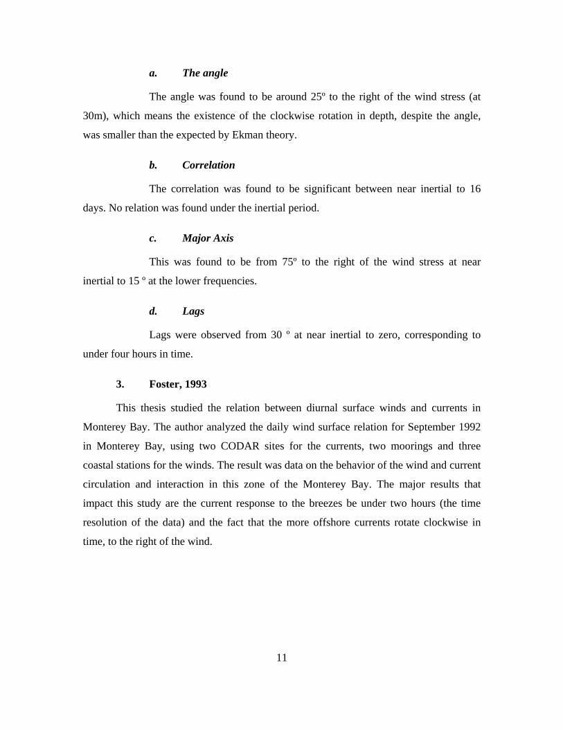
As mentioned earlier, this work is one of the first able to study two long reliable
time series, with continuous one hour measures for more than one year. All data analyzed
was gathered from June 1, 2006 to December 31, 2007. Figure 2 shows the time intervals
for each station. This allows a wide spectrum of possibilities and test scenarios in space
and time, as well as providing outputs of the time series analysis with a very good
resolution, maintaining a continuous information flow with a high confidence level.
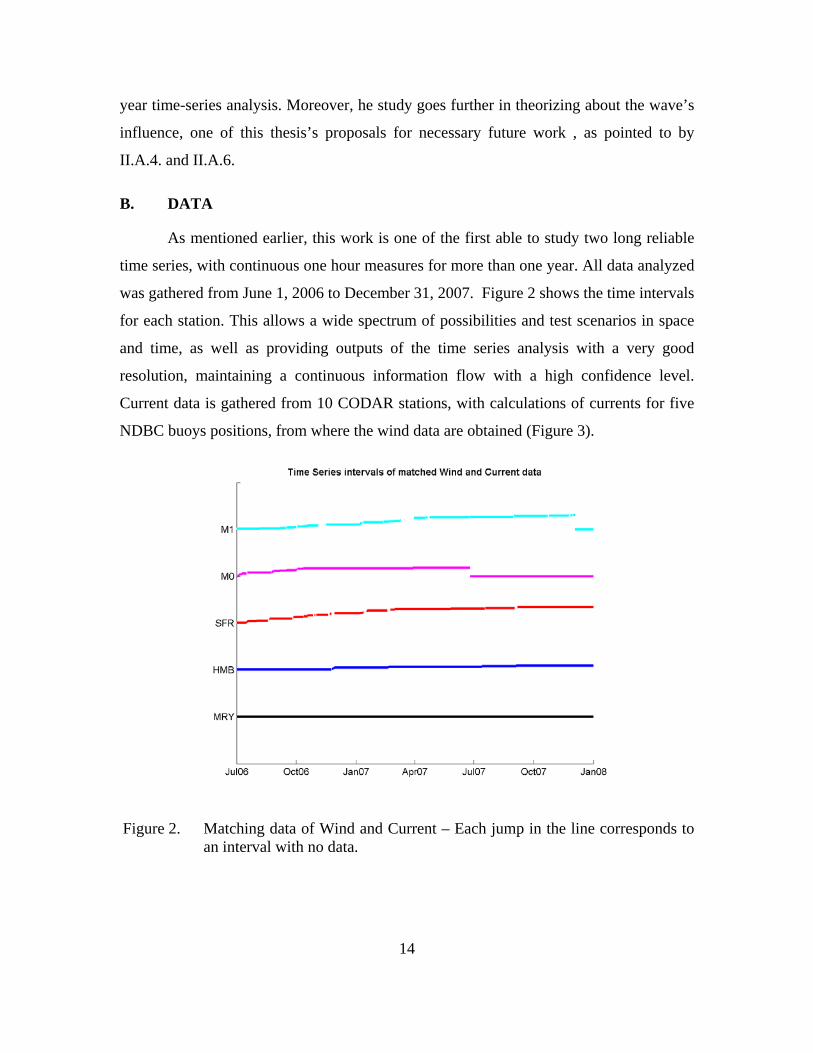
Current data is gathered from 10 CODAR stations, with calculations of currents for five
NDBC buoys positions, from where the wind data are obtained (Figure 3).
Figure 2. Matching data of Wind and Current – Each jump in the line corresponds to an interval with no data.
15
Figure 3. Current and Wind reading stations – Dots represent one example hourly coverage of the Pescadero CODAR station. (From: ArcGIS. Coastline from NOAA, National Ocean Service, 1994.)
1. Winds
Winds were obtained from NOAA’s National Data Buoy Center (NDBC; Figure
4, Table 1), and from the Monterey Bay Aquarium Research Institute (MBARI; Figure 5,
Table 2) moored buoys.
16
a. NDBC Buoys
Figure 4. NDBC type buoy. (From: National Data Buoy Center, http://www.ndbc.noaa.gov, October 2008).
Data from the following NDBC buoys / stations is used:
# Name Distance to shore
Type Position Elevation Anemometer height
Water depth
Watch circle radius
46012 Half Moon Bay (HMB)
4 NM 3 m discus
37.361N 122.881W
sea level
5 m 213.1 m 170 yds
46026 San Francisco (SFR)
18 NM 3 m discus
37.759N 122.833W
sea level
5 m 52.1 m 127 yds
46042 Monterey (MRY)
27 NM 3 m discus
36.753N 122.423W
sea level
5 m 2115 m 2175 yds
Table 1. NDBC Buoys (From: National Data Buoy Center, http://www.ndbc.noaa.gov, October 2008.)
17
b. MBARI Buoys
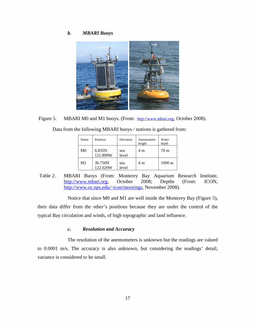
Figure 5. MBARI M0 and M1 buoys. (From: http://www.mbari.org, October 2008).
Data from the following MBARI buoys / stations is gathered from:
Name Position Elevation Anemometer height
Water depth
M0 6.835N 121.899W
sea level
4 m 70 m
M1 36.750N 122.020W
sea level
4 m 1000 m
Table 2. MBARI Buoys (From: Monterey Bay Aquarium Research Institute, http://www.mbari.org, October 2008; Depths (From: ICON, http://www.oc.nps.edu/~icon/moorings, November 2008).
Notice that since M0 and M1 are well inside the Monterey Bay (Figure 5),
their data differ from the other’s positions because they are under the control of the
typical Bay circulation and winds, of high topographic and land influence.
c. Resolution and Accuracy
The resolution of the anemometers is unknown but the readings are valued
to 0.0001 m/s. The accuracy is also unknown, but considering the readings’ detail,
variance is considered to be small.
18
d. Handling
In order to enable treatment and comparison among different equipment
readings, all the data must be formatted into a similar shape. Therefore, all of the wind
time series are:
• Hourly averages of the available 10 minute readings, from the exact hour -30 min to + 30 min;
• Arranged in the form of a three dimensional vector of time (in hours), u velocity (seasonal, in m/s) and v velocity (meridional, in m/s);
• Interpolated for gaps under 6 hours;
• arranged so that seasonality, monthly, synoptic and daily influences are studied by subdivisions of the series in intervals of three months, one month, six days and one day.
• calibrated such that spatial influence is studied by the different locations.
e. Other Series Created
A different time-series is also created for the wind readings of the
Monterey and Half Moon Bay NDBC buoys, where the y axis is rotated for the winds’
largest variance azimuth, maintaining the x axis in perpendicular alignment. This will
serve to interpret the angle between the two major variances of wind and current,
extracting conclusions on interaction both for rotated axis for wind biggest variation only
and for wind data rotated for the wind biggest variation and current to the current biggest
variation.
2. Currents
Currents were obtained from all the in-range CODAR stations, for all the
positions of the wind stations mentioned in the previous section from the buoys positions.
A photograph of a typical CODAR transmit and receive antenna configuration is shown
in Figure 6. Despite the increasing number of CODAR stations around the world, there
have not been many opportunities to operate for a long period with so many stations in a
single study, increasing the number of radial readings for each position. A short
explanation of how CODAR technology appeared and operates is given in paragraph a.
19
a. CODAR Technology
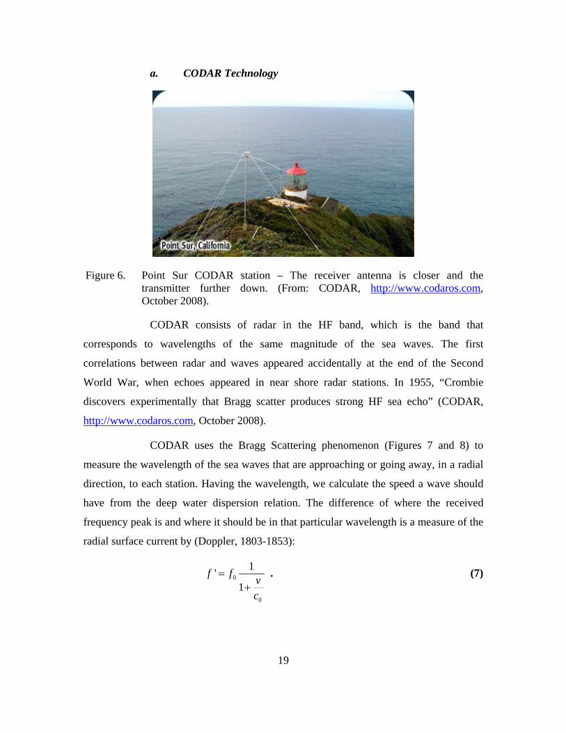
Figure 6. Point Sur CODAR station – The receiver antenna is closer and the transmitter further down. (From: CODAR, http://www.codaros.com, October 2008).
CODAR consists of radar in the HF band, which is the band that
corresponds to wavelengths of the same magnitude of the sea waves. The first
correlations between radar and waves appeared accidentally at the end of the Second
World War, when echoes appeared in near shore radar stations. In 1955, “Crombie
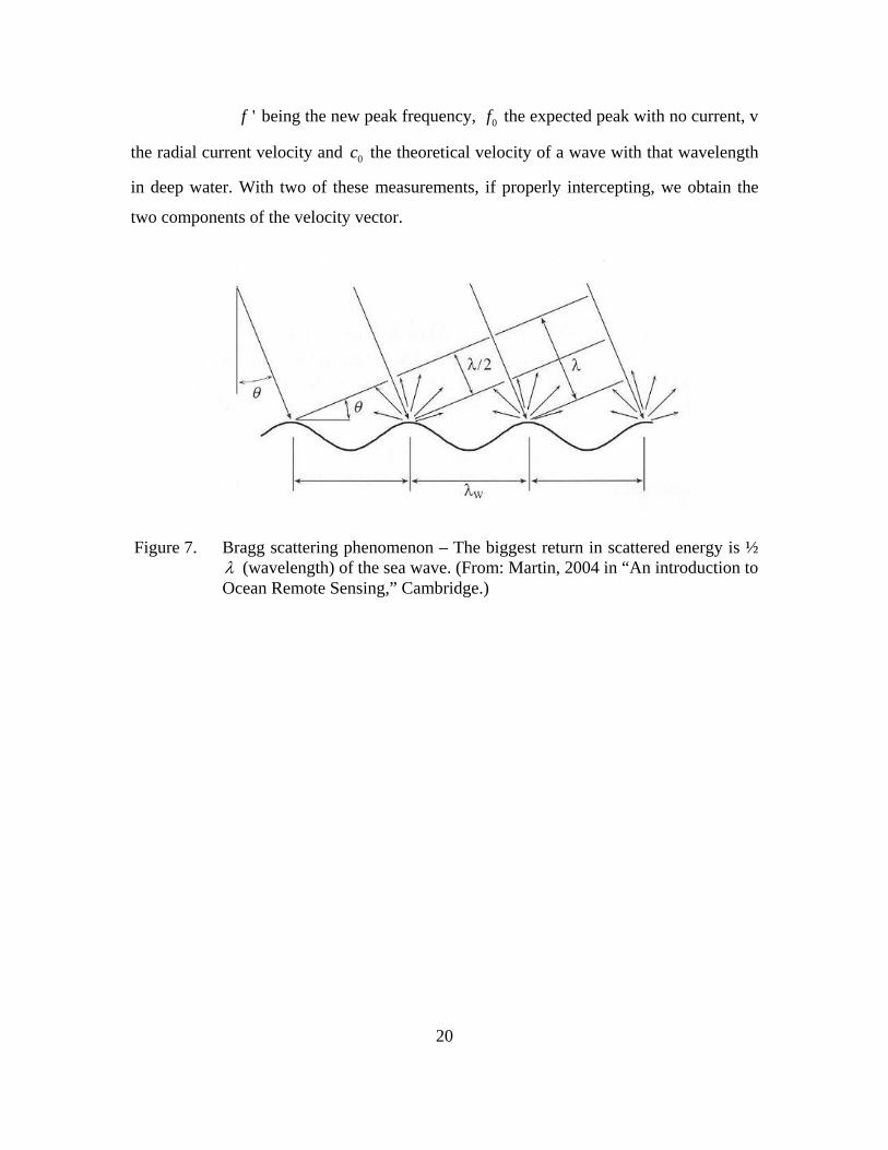
CODAR uses the Bragg Scattering phenomenon (Figures 7 and 8) to
measure the wavelength of the sea waves that are approaching or going away, in a radial
direction, to each station. Having the wavelength, we calculate the speed a wave should
have from the deep water dispersion relation. The difference of where the received
frequency peak is and where it should be in that particular wavelength is a measure of the
radial surface current by (Doppler, 1803-1853):
0
0
1'1
f f vc
=+
. (7)
20
'f being the new peak frequency, 0f the expected peak with no current, v
the radial current velocity and 0c the theoretical velocity of a wave with that wavelength
in deep water. With two of these measurements, if properly intercepting, we obtain the
two components of the velocity vector.
Figure 7. Bragg scattering phenomenon – The biggest return in scattered energy is ½ λ (wavelength) of the sea wave. (From: Martin, 2004 in “An introduction to Ocean Remote Sensing,” Cambridge.)
21
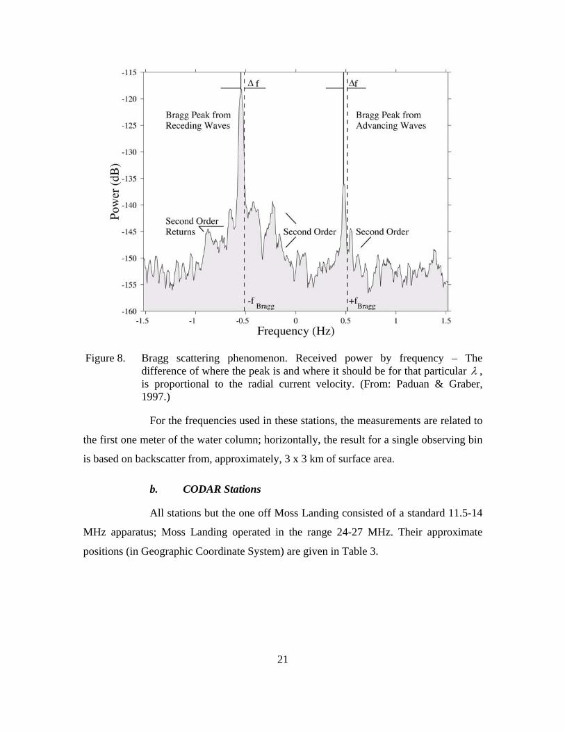
Figure 8. Bragg scattering phenomenon. Received power by frequency – The difference of where the peak is and where it should be for that particular λ , is proportional to the radial current velocity. (From: Paduan & Graber, 1997.)
For the frequencies used in these stations, the measurements are related to
the first one meter of the water column; horizontally, the result for a single observing bin
is based on backscatter from, approximately, 3 x 3 km of surface area.
b. CODAR Stations
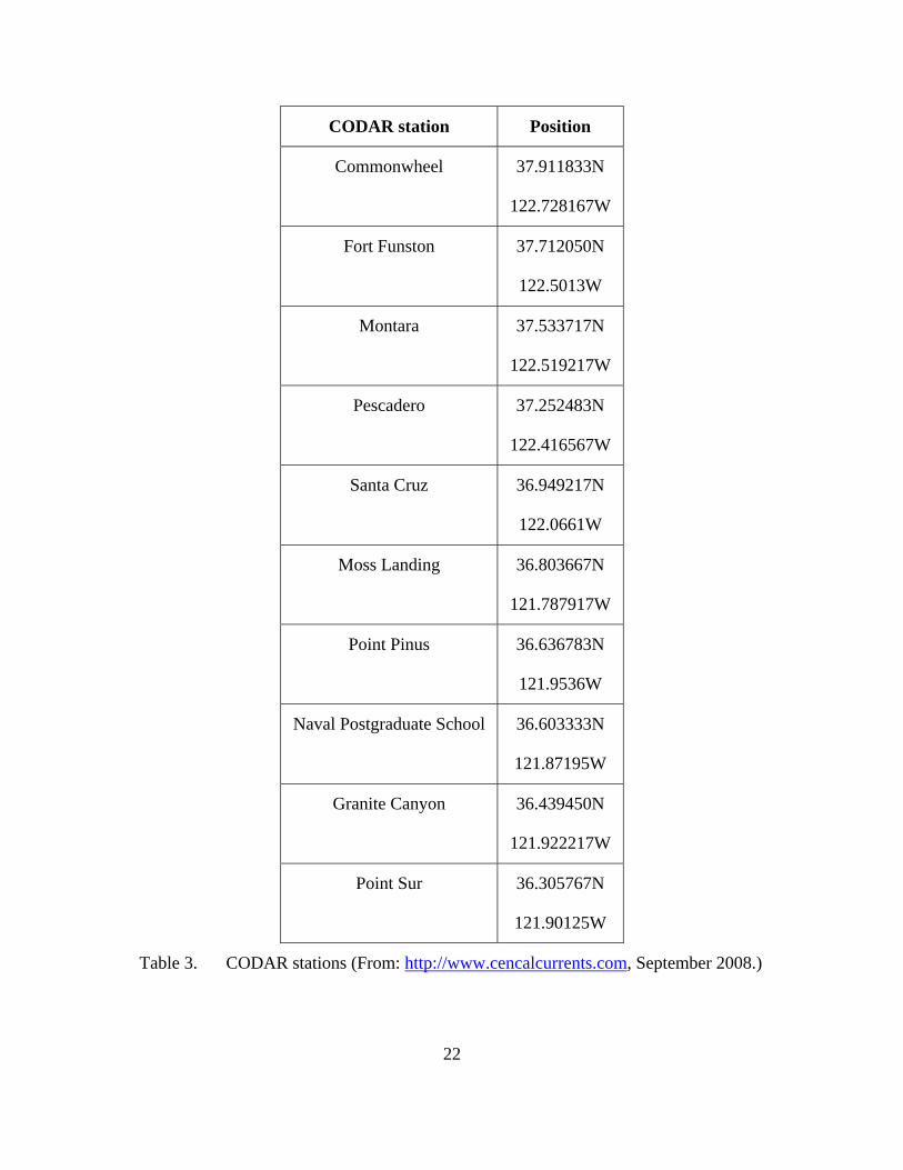
All stations but the one off Moss Landing consisted of a standard 11.5-14
MHz apparatus; Moss Landing operated in the range 24-27 MHz. Their approximate
positions (in Geographic Coordinate System) are given in Table 3.
22
CODAR station Position
Commonwheel 37.911833N
122.728167W
Fort Funston 37.712050N
122.5013W
Montara 37.533717N
122.519217W
Pescadero 37.252483N
122.416567W
Santa Cruz 36.949217N
122.0661W
Moss Landing 36.803667N
121.787917W
Point Pinus 36.636783N
121.9536W
Naval Postgraduate School 36.603333N
121.87195W
Granite Canyon 36.439450N
121.922217W
Point Sur 36.305767N
121.90125W
Table 3. CODAR stations (From: http://www.cencalcurrents.com, September 2008.)
23
c. Resolution and Accuracy
The resolution for these stations is 0.04 m/s (from
http://www.codaros.com, accessed in October 2008). The most recent studies show accuracy
from 8 to 18 cm/s (from Wright, 2008, NPS Masters Thesis).
d. Handling
In order to be able to work with these time series all the data have to be
arranged in a similar fashion. All of the current time series are:
• Hourly averages from the exact hour -30 min to + 30 min, interpolated from the nearest valued positions to the buoys position. This is the way the data is presented by the CODAR system.
• Arranged in the form of a three dimensional vector of time (in hours), u velocity (seasonal, in m/s) and v velocity (meridional, in m/s). This arrangement allows easy handling.
• Interpolated for gaps under 6 hours. This allows a good continuity and guarantees no hiding of important features in the changing of the current.
e. Other Series Created
Other time-series were also created for the current readings of the position
of the Monterey and Half Moon Bay NDBC buoys:
• Where the y axis is rotated for the wind’s largest variance azimuth, maintaining a perpendicular x axis;
• Where the y axis is rotated for the current’s largest variance azimuth, maintaining a perpendicular x axis. (Comparison of the results from steps (1) and (2) also provides information about the most common angle between surface current and wind.)
• All the series created for the Monterey buoy have two more associated scenarios, where the tide influence from the current is tentatively removed. For this purpose the software t_tide is used (Pawlowicz, Beardsley and Lentz, 2002 with a Cook, 2008, alteration to the software). In the first, all of the tide constituents available in the software are used, once this time-series is long enough (in this case, one and a half years). In the second one, all but the S1 constituents are used, in order to avoid removing the sea breeze influence. In both we have to take into account that the energy removed may not be just tide related, as occurs in periods of the order of the rotation of the planet’s rotation frequency.
24
• Seasonality, monthly, synoptic and daily influences are studied by subdivisions of the series in intervals of three months, one month, six days and one day.
• Spatial influence is studied by the different locations.
3. Both Wind and Current
The time series of both wind and current are then cut in order to create time
intervals where they both exist, to make comparison possible. The resulting matched
intervals are displayed in Figure 2.
From now on in this thesis, for reference simplicity, when a station is mentioned
by place name it refers to the buoy position; e.g., “Monterey Station” means the data
obtained for the position of the 46042 NDBC buoy. Because the Monterey station has a
broader continuous time series, it allows us to extrapolate more results with a better
resolution. That particular location is where most studies and essays are made, the others
serving as comparisons.
C. EMPIRICAL APPROACH
Two independent paths are taken. The first starts with real data and tries to
extrapolate relations from it. This approach relies on pure Time Series Analysis. The
second, described in II D., is based on theoretical knowledge and serves as comparison to
the empirical results.
All of the following methods are applied in all of the time series described in B.
1. Principal Axis (Biggest Variance)
The objective is to have a measure of the axis which experiences the largest
variance and its angle of measurement, for both wind and current. The result is plotted as
Figure 9 and as a table in Table 4, where the two major semi-axes in the along vector
direction are shown in full (using Bahr, 2007, software):
25
−3 −2 −1 0 1 2 3−3
−2
−1
0
1
2
3
U
V
Elipses axis from 01−Jul−2006 + 1.5 years : alfa=−58.5547deg
Wind (m/s)Current (dm/s)
Figure 9. Principal axis analysis – Values correspond to variance and alfa is the angle between the two full lines. (Monterey station.)
The table shows values for each term:
Principal axis for W/C: from 01-Jul-2006 + 1.5 years
theta Maj. min.
wind -30.4301 4.8623 1.9311
current 28.1246 0.13539 0.13232
Table 4. Principal axis analysis. – Values correspond to magnitudes and angle between the major axis and north. (Monterey station.)
The results of all the time series show that magnitudes of the variance keep within
the same order. The angles vary more, getting dispersed as we reduce the time series
length. The average angle between the two major variance directions is around 50
degrees in the longer time-series as shown in Table 5.
26
Examples of results from the different stations in different periods
Station Period Angle between major axis (º)
MRY 01JUL06 .. 31DEC07 -59
HMB 01JUL06 .. 23NOV06
20FEB07 .. 12JUL07
04SEP07 .. 31DEC07
-14
-8
-10
SFR 29NOV06 .. 07JAN07
01MAR07 .. 26MAY07
06SEP07 .. 31DEC07
-2
-15
-19
M0 11OCT06 .. 28MAR07
29MAR07 .. 25JUN07
25JUN07 .. 31DEC07
-39
+21
+25
M1 16NOV06 .. 05JAN07
24APR07 .. 24JUN07
25JUN07 .. 30AUG07
-43
+1
-6
Table 5. Principal axis analysis. – Space and time variability (wind – current.)
Despite the tendency for the longer time series, the high variability does not allow
a good estimation of a typical angle between wind and current, demonstrating that it may
be more a function of time and place.
2. Complex Correlation (Kundu, 1975)
Complex correlation gives a measure of correlation between two complex time
series. The magnitude of the result shifts between 0 and 1, 1 being if the signal is the
same. The average phase angle gives an idea of the physical angle between the two
phenomena. Results for the Monterey station are plotted on Figure 10, and results for all
stations are tabulated in Table 6.
27
−1 −0.8 −0.6 −0.4 −0.2 0 0.2 0.4 0.6 0.8 1−1
−0.8
−0.6
−0.4
−0.2
0
0.2
0.4
0.6
0.8
1Complex Correlation W/C MRY JUL06 to DEC07
Real
Imag
mod=0.48542 alfa=−31.7407
Figure 10. Complex correlation – Modulus is a measure of correlation and alpha is the physical angle. (Monterey station.)
The magnitudes vary from 0.2 to 0.7. The angles tend to remain on the second
quadrant around 35 degrees, gaining variance with the reducing of the length of the time
series. These results mean that they are correlated, and there is in average 35 degrees
between the directions of the two. This is expected because the angle is supposed to
increase in time, until Ekman’s 45 degrees. The results for M0 buoy present the highest
variability but also the smaller correlation, probably due to the variability of the winds
and currents inside the Bay. An attempt was made to verify if the correlation would
increase when lagging the Current time series, but it decreased, pointing to zero lag.
Examples of results from the different stations in different periods
Station Period Magnitude Angle (º)
MRY 01JUL06 .. 31DEC07 0.49 -32
HMB 01JUL06 .. 23NOV06
20FEB07 .. 12JUL07
04SEP07 .. 31DEC07
0.31
0.66
0.48
-56
-47
-56
SFR 29NOV06 .. 07JAN07
01MAR07 .. 26MAY07
06SEP07 .. 31DEC07
0.66
0.81
0.62
-1
-16
-23
28
Station Period Magnitude Angle (º)
M0 11OCT06 .. 28MAR07
29MAR07 .. 25JUN07
25JUN07 .. 31DEC07
0.34
0.27
0.17
-26
-83
-45
M1 16NOV06 .. 05JAN07
24APR07 .. 24JUN07
25JUN07 .. 30AUG07
0.5
0.67
0.69
-34
-17
-13
Table 6. Complex correlation. – Space and time variability.
3. Scatter Comparison
Scatter plots give an idea of correlation and permit a mathematical best-fit
expression (e.g., Figure 11, Figure 12, Figure 13). A perfect correlation happens when all
the pairs of values (points) of the two time series design a mathematical expression. This
will allow elaboration of the best transfer function relation in terms of magnitude. The
one presented here considers the full energy spectrum, and the best fit is accomplished
with a quadratic expression.
This analysis can also be done by frequency bands if the choice is to transfer by
frequency. As we will see later, the degree of added complexity for such an approach will
not increase significantly the results of the first one.
29
Figure 11. Scattering diagram for U and best fit expression. (Monterey station, Jul 06 to Dec 07.)
Figure 12. Scattering diagram for V and best fit expression. (Monterey station, Jul 06 to Dec 07.)
30
Figure 13. Scattering diagram for Modulus and best fit expression. (Monterey station, Jul 06 to Dec 07.)
After applying it to all the series, including the rotated ones, the best proxy for the
typical expression relating near surface wind to surface current, in terms of magnitude of
the vector, is:
50.018 0.03C U= + (8)
where C is the surface current in m/s and U5 is the wind at 5 m height, also in m/s.
The quadratic term shown on the figures is always positive and negligible, with
some exceptions in the modulus when it goes negative. The results presented here are
restricted to the linear terms in the fit. Those values multiplying by U5 vary plus or minus
0.02. But, overall, the results show surface current magnitudes are very close to 2% of the
wind speed magnitudes (Table 7). The choice of 0.018 is supported by the error analysis
and tuning done in the forecast section. The last constant varies plus or minus 0.05. This
variation tends to be smaller in winter and fall and in the fits based on longer time series.
This expression will be tuned in the predicting algorithm in Section III.
31
Examples of results from the different stations in different periods
Table 7. Best fit expression. – Space and time variability.
4. Auto Correlation (McMahan and Wyland, NPS Lab Software, 2007)
Autocorrelation of a given time series allows for a better understanding of the
time scales involved. Each oscillation represents the time scale of an active agent.
Examples are shown for wind and current in Figure 14 and Figure 15, respectively.
32
Figure 14. Autocorrelation for Wind – The bottom is a zoom of the first positive 2000h ~ 3 Months. Daily, synoptic and monthly oscillations are present. (Monterey station, Jul 06 to Dec 07.)
33
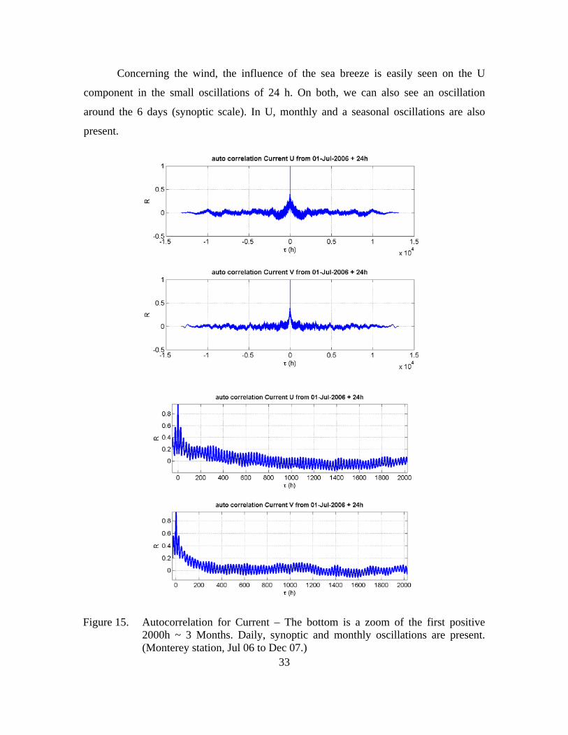
Concerning the wind, the influence of the sea breeze is easily seen on the U
component in the small oscillations of 24 h. On both, we can also see an oscillation
around the 6 days (synoptic scale). In U, monthly and a seasonal oscillations are also
present.
Figure 15. Autocorrelation for Current – The bottom is a zoom of the first positive
2000h ~ 3 Months. Daily, synoptic and monthly oscillations are present. (Monterey station, Jul 06 to Dec 07.)
34
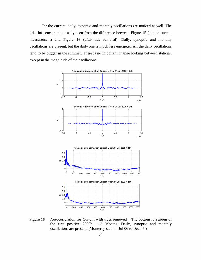
For the current, daily, synoptic and monthly oscillations are noticed as well. The
tidal influence can be easily seen from the difference between Figure 15 (simple current
measurement) and Figure 16 (after tide removal). Daily, synoptic and monthly
oscillations are present, but the daily one is much less energetic. All the daily oscillations
tend to be bigger in the summer. There is no important change looking between stations,
except in the magnitude of the oscillations.
Figure 16. Autocorrelation for Current with tides removed – The bottom is a zoom of
the first positive 2000h ~ 3 Months. Daily, synoptic and monthly oscillations are present. (Monterey station, Jul 06 to Dec 07.)
35
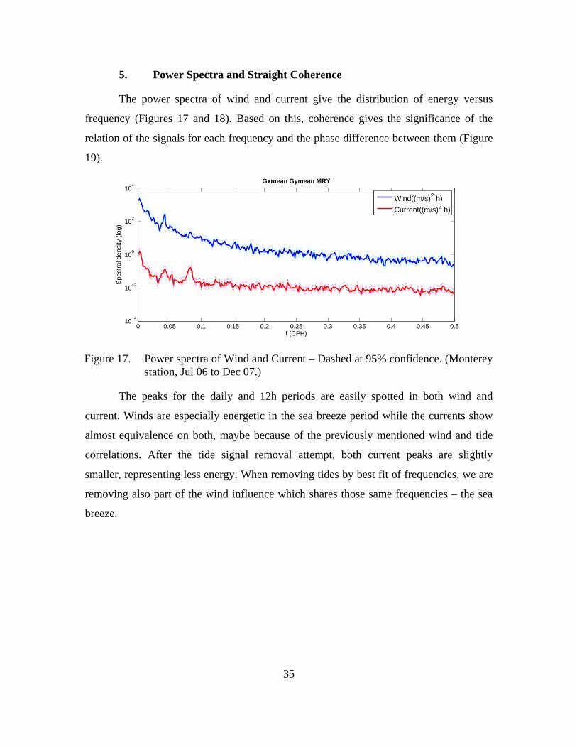
5. Power Spectra and Straight Coherence
The power spectra of wind and current give the distribution of energy versus
frequency (Figures 17 and 18). Based on this, coherence gives the significance of the
relation of the signals for each frequency and the phase difference between them (Figure
19).
0 0.05 0.1 0.15 0.2 0.25 0.3 0.35 0.4 0.45 0.510
−4
10−2
100
102
104
f (CPH)
Spe
ctra
l den
sity
(lo
g)
Gxmean Gymean MRY
Wind((m/s)2 h)
Current((m/s)2 h)
Figure 17. Power spectra of Wind and Current – Dashed at 95% confidence. (Monterey station, Jul 06 to Dec 07.)
The peaks for the daily and 12h periods are easily spotted in both wind and
current. Winds are especially energetic in the sea breeze period while the currents show
almost equivalence on both, maybe because of the previously mentioned wind and tide
correlations. After the tide signal removal attempt, both current peaks are slightly
smaller, representing less energy. When removing tides by best fit of frequencies, we are
removing also part of the wind influence which shares those same frequencies – the sea
breeze.
36
0 0.05 0.1 0.15 0.2 0.25 0.3 0.35 0.4 0.45 0.510
−4
10−2
100
102
104
f (CPH)
Spe
ctra
l den
sity
(lo
g)
Tides out − Gxmean Gymean MRY
Wind((m/s)2 h)
Current((m/s)2 h)
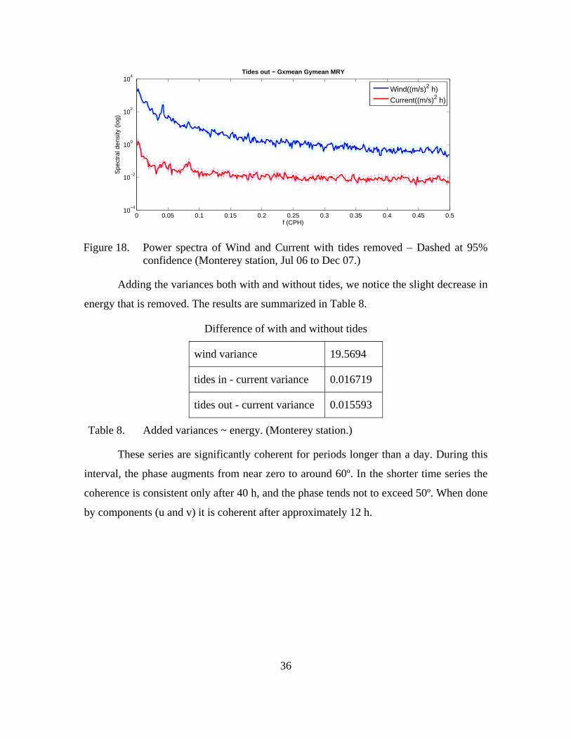
Figure 18. Power spectra of Wind and Current with tides removed – Dashed at 95% confidence (Monterey station, Jul 06 to Dec 07.)
Adding the variances both with and without tides, we notice the slight decrease in
energy that is removed. The results are summarized in Table 8.
Tides in − Coherence for MRY from 01−Jul−2006 + 1.5 years
coherencesign.level 0.95
−0.08 −0.06 −0.04 −0.02 0 0.02 0.04 0.06 0.08
−100
0
100
f (CPH)
Phase
(deg
)
Figure 24. Complex Coherence and Phase – Lower image is a zoom of the coherent part. (Monterey station, Jul 06 to Dec 07.)
The application of this method allows one to calculate, besides the coherence, the
angular shift in time. Table 9 shows the average results for the coherent-positive part.
41
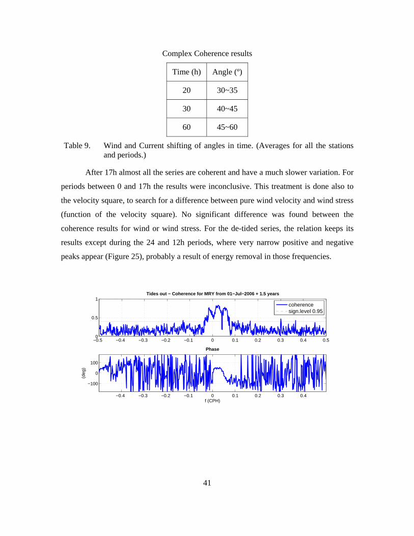
Complex Coherence results
Time (h) Angle (º)
20 30~35
30 40~45
60 45~60
Table 9. Wind and Current shifting of angles in time. (Averages for all the stations and periods.)
After 17h almost all the series are coherent and have a much slower variation. For
periods between 0 and 17h the results were inconclusive. This treatment is done also to
the velocity square, to search for a difference between pure wind velocity and wind stress
(function of the velocity square). No significant difference was found between the
coherence results for wind or wind stress. For the de-tided series, the relation keeps its
results except during the 24 and 12h periods, where very narrow positive and negative
peaks appear (Figure 25), probably a result of energy removal in those frequencies.
−0.5 −0.4 −0.3 −0.2 −0.1 0 0.1 0.2 0.3 0.4 0.50
0.5
1Tides out − Coherence for MRY from 01−Jul−2006 + 1.5 years
coherencesign.level 0.95
−0.4 −0.3 −0.2 −0.1 0 0.1 0.2 0.3 0.4
−100
0
100
f (CPH)
Phase
(deg
)
42
−0.5 −0.4 −0.3 −0.2 −0.1 0 0.1 0.2 0.3 0.4 0.50
0.2
0.4
0.6
0.8
1Tides out but S1 − Coherence for MRY from 01−Jul−2006 + 1.5 years
coherencesign.level 0.95
−0.4 −0.3 −0.2 −0.1 0 0.1 0.2 0.3 0.4
−150
−100
−50
0
50
100
150
f (CPH)
Phase
(deg
)
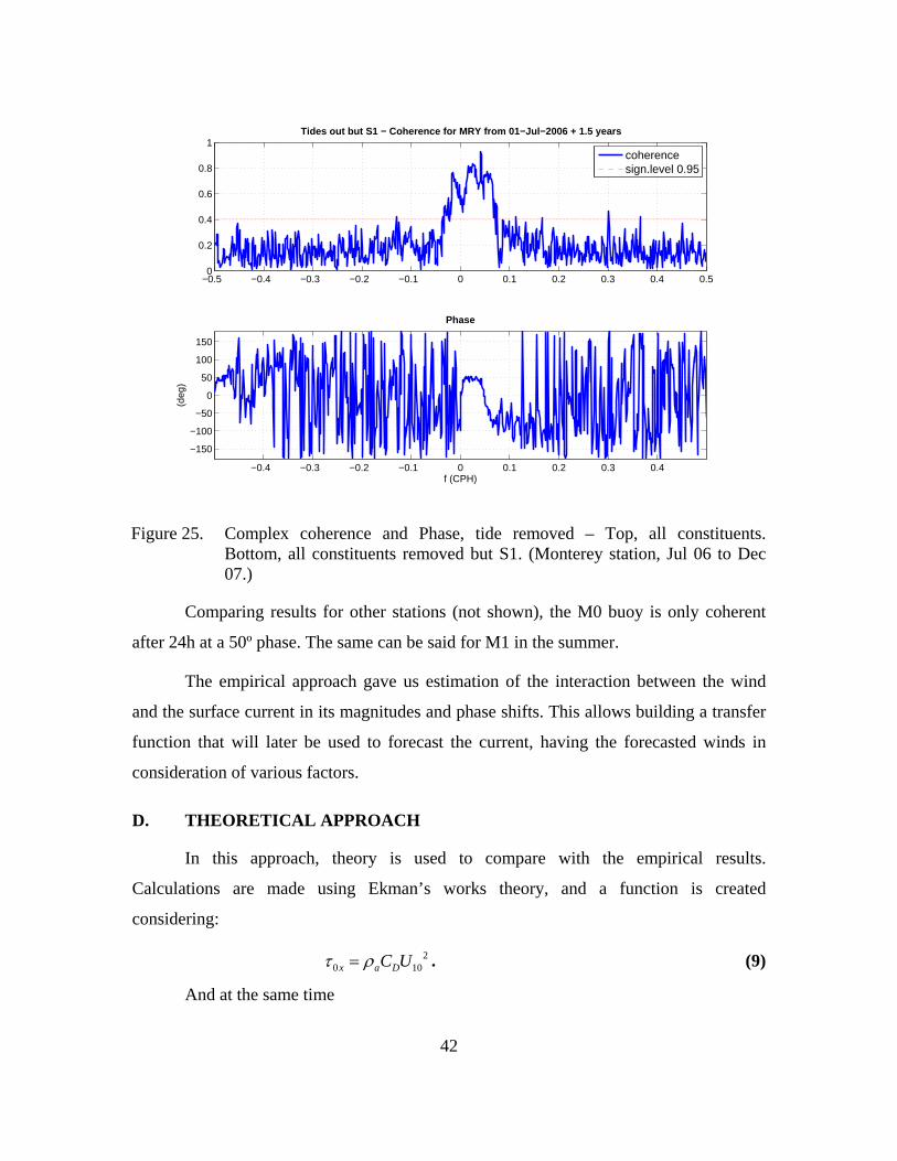
Figure 25. Complex coherence and Phase, tide removed – Top, all constituents. Bottom, all constituents removed but S1. (Monterey station, Jul 06 to Dec 07.)
Comparing results for other stations (not shown), the M0 buoy is only coherent
after 24h at a 50º phase. The same can be said for M1 in the summer.
The empirical approach gave us estimation of the interaction between the wind
and the surface current in its magnitudes and phase shifts. This allows building a transfer
function that will later be used to forecast the current, having the forecasted winds in
consideration of various factors.
D. THEORETICAL APPROACH
In this approach, theory is used to compare with the empirical results.
Calculations are made using Ekman’s works theory, and a function is created
considering:
20 10x a DC Uτ ρ= . (9)
And at the same time
43
x a VuAz
τ ρ ∂=
∂. (10)
So, adding the two and rearranging,
210
0
a D
V
Cu z UA
ρρ
∂ = ⋅∂ ⋅ . (11)
The magnitude of U10 is taken to be approximate of U5, for it is the top part of the
exponential wind growth in height; the Yelland and Taylor, 1995 drag coefficient is used
as function of the wind speed.
E. COMPARISON
Having the empirical and the theoretical result transfer functions, and using U10 =
10 m/s we obtain:
1. From the results of the study in equation (8),
du=0.21 m/s.
2. From the theoretical result of (11),
a. Ekman depth = 50m and AV=0.01 m2/s du=0.68 m/s;
b. Ekman depth = 10m and AV=0.01 m2/s du=0.27 m/s;
c. Ekman depth = 50m and AV=0.3 m2/s du=0.02 m/s;
d. Ekman depth = 10m and AV=0.3 m2/s du=0.01 m/s.
This means that the theoretical result is highly dependent on a good estimate of
eddy viscosity, and that using a typical value (Av~0.01), Ekman depth must be much
shallower. Using typical values, Ekman theory overestimates the change in the surface
current velocity.
F. CONCLUSIONS
Having studied the wind / surface current interaction in different perspectives,
times and spaces, the relationship found can be described as follows.
44
1. Transfer Function
a. Magnitude
The surface current generated is around 2% of the wind speed.
b. Angle
The angle measurement increases in an unknown way until around 17h.
From then on, the angles vary from 35º to 60º, according to Table 9.
2. Notes
Despite these results, the scatter plots show a large dispersion, which means that
there is a high variability.
The unknown growth until 17h includes wind wave interaction. It includes also
components of transfer from 0 to 35º of some magnitude.
In this study, rotating the axis to biggest variance or long-shore, cross-shore, does
not bring any significant change, probably because of the meridional characteristic of the
Californian coast. Nevertheless, when using both wind and current axis to their respective
biggest variances, the component minor wind axis versus minor current axis does tend to
zero.
The tidal removal does not bring major changes to the transfer function as a bulk.
If transferred by frequency, care has to be taken especially in the inertial periods and its
subdivisions.
45
III. THE FORECAST
A. FORECAST WITH CODAR
Forecasting with a remote sensing means like CODAR has the enormous
advantages of independence and timing--independence because it does not rely on any
other system to operate, and timing because it is updated every hour. This is more than
enough to get good estimates for the surface currents variability, making data available
when needed. Nevertheless, relying only on previous surface currents readings from our
own system has its dangers and limitations. As will be shown, coupling our readings with
those of other systems yields more reliable and accurate results.
1. Reliability of a Forecast
CODAR has proved to be a very reliable system, so far. Nevertheless, its results
may be misleading. Once it uses electromagnetic radiation to operate, it is subject to all
its difficulties and laws, as described by the following examples.
• If an object with electromagnetic potential and length comparable to the transmitted wavelength (approximately 10m) goes near the antennas, the reception pattern changes, leading to deviation in the result;
• The presence of a moving target, such as a ship, may introduce an error due to strong backscatter;
• A change in the background radio frequency properties will influence the signal also.
These and other problems have been addressed several times, and are adequately
explored in several works (some of which can be found on http://www.codaros.com). The
use of a second system allows us to detect possible malfunctions by comparison, and
gives a different set of solutions as backup. This is always preferable.
2. Accuracy of a Forecast
The accuracy of the system is dependent on the errors of CODAR (8 to 18 cm/s,
from Wright, 2008), plus the ones associated with the estimation of the next 24h behavior
(the assumptions and the errors of the systems we are building our prognostic on), plus
46
the error of what we cannot or do not predict. If we introduce to our algorithm a good
description of the future conditions and have good relation functions, we will obtain a
more realistic result.
So, coupling with other systems, as upload or download, is advantageous. We can
obtain data from tides, winds, drifters, current meters, and models--and can assimilate our
results back into the models.
B. PREVIOUS ATTEMPTS
The previous attempt model is described in I B. The results have been generally
accurate for persistent weather conditions, but tend to get worse with changing weather
conditions.
1. Problems
The model was based only in tidal and persistence analysis. Once any of the
conditions--wind, waves, or any other parameter--changes, the persistence does not
follow. In weather, significant changes can happen in any 24h period.
2. Results
As pointed in I.B., there is still lack of confidence in this model any time there is a
significant change in the weather (namely in current velocity and possibly wind). A
summary of results for the previous tidal model applied to the region offshore San
Francisco is shown in Figure 26. Here a pixel grid of pseudo drifters release points was
used to create predicted trajectories for 24h, which was repeated each hour for the period
August 2006 through July 2007. The plot shows the rms spatial difference between the
end points of the predicted trajectories compared with the observed trajectories one day
after. The negative correlation with number of drifters (lower panel) reflects the fact that
higher speed conditions result in more pseudo drifters, leaving the sampling grid within a
24h period. The direct effect of wind speed on the spatial accuracy of the predicted
trajectories is less clear. Nonetheless, wind (specifically wind changes) is hypothesized to
explain some error in forecast currents.
47
0 5 10 15 20 25 30 35
2
4
6
8
10
12
14
16
18
Win
d S
peed
(m
/s)
0
50
100
150
200
250
300
350W
ind
Ang
le (
deg)
0 5 10 15 20 25 30 3510
20
30
40
50
60
70
RMS Separation Distance (km)
Num
ber
(max
=74
)
Figure 26. Results for RMS compared with wind and number of pseudo drifters – RMS for 24h. The number of pseudo drifters present may be used as a proxy for current speed. (Image from Garfield et al., 2007.)
C. THE INTRODUCTION OF WIND
One attempt to reduce forecast error is the introduction of wind influence. A study
of the wind surface / current interaction was made for this thesis and is described in
Section II. The objective was to build a transfer function that allows us to plug in the
wind driven current into the forecast. Several approaches were considered: transfer by
48
frequency, transfer by different division of spatial and time components, transfer as a
vector, transfer with tide analysis, and transfer based on persistence. The approaches that
seemed to be more efficient for practical purposes (accuracy versus simplicity) narrowed
to only one wind/current transfer function and transfer as a vector. Transfer by frequency
was not chosen because of the relatively small magnitude of the end results. Tide removal
and simple persistence conditions would have yielded similar results. The models tested
were based on the diagram in Figure 27, regardless whether or not tides were removed.
The winds had different methodologies applied also in terms of what time slice
constituted future for computing wind differences and whether or not to use wind
difference compared with removing and then reintroducing the full wind-driven current.
The results were practically the same. In this hindcast study, forecast wind is taken from
the actual readings, simulating a zero error wind forecast. The methodology tested here
can, however, be immediately transferred to winds forecasted by an atmospheric model
such as the Navy's COAMPS model.
Figure 27. Basic flow chart diagram of the forecast procedure – Several adaptations were attempted.
1. With Tides Treatment
This attempt corresponds exactly to the previous diagram. The best results were
obtained using the following procedure.
We are at t=0 and we want the next 24h surface currents forecast, so we
49
• Take the last 24h current readings;
• Remove the tides by “t_tide” using all the previous month’s currents to the best fit. Conducting the detiding with using one month of data or just three days of data both returned good results as shown in Table 10.
Detidal associated errors
RMS (m/s) 3 Days 1 Month
U 0.1087 0.1073
V 0.1027 0.1145
modulus 0.1515 0.1593
Table 10. Detidal errors with 3 days and 1 Month data – The calculation of the Root Mean Square error will be discussed in III. E. (Monterey Station.)
• Forecast the tide for the next 24h using “t_predic” and the structure of constituents that resulted from the detiding;
• Low pass filter the residual current to 18h;
• Average the residual current;
• Take the last 24h wind readings;
• For each hour in the future h, get the forecast wind from that hour until t=0 and the wind readings before that until h-24;
• Low pass filter both to 18h;
• Do the average for each;
• Take the difference of the winds;
• Use the transfer function to get the current associated with the wind difference;
• Sum the residual current, the tide and the wind current.
Figure 28 is an example of the obtained result, in a day where a major wind
change took place and the wind influence is noted. The resolution is hourly.
Figure 31. Relation of RMS error and the stations – Top is magnitude of the current vs. error. Bottom is variability vs. error. Based on the tide plus mean with transfer function model forecasts.
55
Seasonality does not seem to play a major role, but the small quantity of data does
not allow a definitive conclusion. The four-season results for the Monterey station are
shown in Figure 32.
0.135 0.14 0.145 0.15 0.155 0.16 0.1650.155
0.16
0.165
0.17
0.175
0.18
0.185
0.19
Error magnitude (m/s)
Cur
rent
mag
nitu
de (
m/s
)
Seasonally
0.065 0.07 0.075 0.08 0.085 0.09 0.095 0.10.168
0.17
0.172
0.174
0.176
0.178
0.18
0.182
0.184Variability Seasonally
Error magnitude (m/s)
Var
iabi
lity
at 9
5% (
m/s
)
Figure 32. Relation of RMS error and seasons – Top is magnitude of the current vs. error. Bottom is variability vs. error. (For Monterey station, based on the tide plus mean wind transfer function forecasts.)
The long records from the Monterey station can be used to illustrate the temporal
behavior of the forecast error and the influence of the wind-based corrections. The daily
RMS current speed errors are plotted in Figure 33 with and without the wind-based
corrections. Almost everywhere, the wind-treated forecasts, blue and black, are lower.
Red and green tips are easily seen constantly at the top, despite the small difference.
Figure 36. Zoom of RMS versus SWH, current and wind – High error seems associated with large current variation. Top with tides treatment. Bottom with persistence. (Monterey station.)
62
THIS PAGE INTENTIONALLY LEFT BLANK
63
IV. CONCLUSIONS
This study analyzed long records of HF radar-derived surface currents and
mooring-based wind observations for the region offshore Monterey Bay, California. The
growth of HF radar instrumentation and the resulting surface current mapping data has
enabled a number of scientific and public safety capabilities. In many instances,
particularly with respect to search and rescue or spill mitigation applications, surface
current forecasts are critical in addition to real time observations. To make accurate
forecasts requires knowledge of background flow patterns plus variable flow patterns
related to tides and wind-driven currents. The focus here has been on created and testing
models for wind-driven surface currents that are specific to the near-surface (~0.5m)
depths of the HF radar observations.
The Monterey Bay region contains a wealth of surface observations from both HF
radar and meteorological buoys. One site, in particular, surrounding the NOAA/NDBC
buoy 46042 location has provided an eighteen-month, continuous set of currents and
winds. Those data were used to develop an empirical transfer function between wind and
HF radar-derived current. Shorter data sets from other buoy sites both inside and outside
Monterey Bay were used to confirm results from the buoy 46042 location. In addition to
the forward problem of creating a best-fit transfer function from wind to current, the
recommended parameters were adjusted slightly by determining which values provided
the most accurate 24-hour forecast of HF radar-derived surface current at the buoy 46042
location. The results of these wind versus surface current analyses from the 1.5 year
dataset from five different stations lead to the following conclusions and requirements.
A. THE WIND INFLUENCE
The wind induced current is on the order of 2% of the total wind speed, which is
consistent with historical values. Despite this magnitude, the influence of introducing an
explicit wind-driven current correction to the existing mean plus tidal current forecast
models leads to around 10% of increased accuracy in the forecasts. The best results are
obtained with a 50º clockwise rotation, and with a magnitude 50.018 0.018windC U= + .
64
Although this study has shown a clear benefit to including a wind-driven correction, this
correction is still below the level of the forecast uncertainties that derives from other
uncorrected factors.
B. RESULT CAPABILITIES
The overall result, including the wind-driven current correction, shows that HF
radar-derived surface current mapping data are able to forecast surface currents in the
next 24h with errors of about 0.15 +/- 0.1 m/s with 95% confidence. When significant
changes in current happen without the wind influence, approximately one day of high
RMS forecast error is expected. The largest and most persistent error events for the test
period from July 06 to December 07 led to a four-day RMS error over 0.2 m/s.
C. NEXT STEPS
The goal here has been to develop improvements to the short-term surface current
forecast model, with primary focus on included the effects of predicted wind changes.
Several other factors that are expected to influence the accuracy of 24-hour surface
current forecasts were pointed out in Chapter III. The results here show that it will be
necessary to understand and incorporate more of those influences if improvements
beyond the 10% level achieved here are desired. The qualitative assessment of error
sources presented in the last chapter, combined with previous work on HF radar surface
current validation, suggests that errors in the measurements themselves may still be the
biggest limitation to improved forecasts.
In addition to work that is ongoing to improve HF radar surface currents and error
tracking, this study points to the need to begin to incorporate the most important aspect of
HF radar observations into the forecast process. That is, spatial information from the
surface current mapping data should be incorporated. At this time, all information about
the sub tidal, tidal, and wind-driven surface currents that goes into the forecast models
derives from time series information from a single location. HF radar, on the other hand,
provides a map of surface currents every hour. Observations show those maps contain a
good deal of horizontal variation in the surface currents, which is the fundamental reason
that a network of HF radar systems is necessary for the transport applications supported
65
here compared with, for example, a single, moored current meter. The next generation
forecast models should account for advective effects. The use of spatial integration
between one calculated point and its immediate neighbors may allow gross errors to
emerge more clearly.
66
THIS PAGE INTENTIONALLY LEFT BLANK
67
LIST OF REFERENCES
Ardhuin, F., B. Chapron, T. Elfouhaily, 2003: Waves and the Air-sea Momentum Budget: Implications for Ocean Circulation Modeling. Journal of Physical Oceanography (2004), 34, 1741-1755.
Ardhuin, F., L. Marié, N. Rascle, P. Forget, A. Roland, 2008: Observation and estimation of Lagrangian, Stokes and Eulerian currents induced by wind and waves at the sea surface. French Service Hydrographique et Océanographique de la Marine, Ifremer, Université du Sud Toulon-Var and German Technishe Universitat Darmstadt. (Not yet published. Manuscript in final form).
CODAR Ocean Sensors, 2008: References, bibliography and station picture. http://www.codaros.com (accessed September 2008).
Ekman, V., 1905: On the influence of the Earth’s rotation on ocean-currents. Arkiv for Matematik, Astronomi och Fysik, 2 (11), 1-52.
Emery, W., D. Matthews, D. Baldwin, 2005: Mapping Surface Coastal Currents with Satellite Imagery and Altimetry. Environmental research, engineering and management, 2(32), 25-29.
Foster, M., 1993: Evolution of Diurnal Surface Winds and Surface Currents for Monterey Bay. Master Thesis, Naval Postgraduate School.
Garfield, N., J. Paduan, C. Ohlmann, 2007: Delivery and Quality Assurance of Short-Term Trajectory Forecasts from HF Radar Observations. Progress report submitted to the Coastal Response Research Center.
Gonella, J., 1972: A rotary-component method for analyzing meteorological and oceanographic vector time series. Deep-Sea Research, 19, 833-846.
Kundu, P., 1975: Notes and Correspondence – Ekman Veering Observed near the Ocean Bottom. Journal of Physical Oceanography, 6, 238-242.
Martin, S., 2004: An Introduction to Ocean Remote Sensing. Cambridge, 266pp.
McNally, G., D. Luther, W. White, 1988: Subinertial Frequency Response of Wind-Driven Currents in the Mixed Layer Measured by Drifting Buoys in the Midlatitude North Pacific. Journal of Physical Oceanography, 19, 290-300.
Monismith, S., E. Cowen, H. Nepf, J. Magnaudet, L. Thais, 2006: Laboratory observations of mean flows under surface gravity waves. Journal of Fluid Mechanics (2007), 573, 131-147.
68
Monterey Bay Aquarium Research Institute, 2008: Data and buoy pictures. http://www.mbari.org (accessed from March to September 2008).
Mooers, C., 1973: Instruments and Methods – A technique for the cross spectrum analysis of pairs of complex-valued time series, with emphasis on properties of polarized components and rotational invariants. Deep-Sea Research, 20, 1129-1141.
National Oceanic and Atmospheric Administration, 2008: Data and buoy pictures. http://ndbc.noaa.gov (accessed from March to September 2008).
O’Donnell, J., D. Ullman, M. Spaulding, E. Howlett, T. Fake, P. Hall, T. Isaji, C. Edwards, E. Anderson, T. McClay, J. Kohut, A. Allen, S. Lester, C. Turner, M. Lewandowski, 2005: Integration of Coastal Ocean Dynamics Application Radar (CODAR) and Short-Term Predictive System (STPS) Surface Current Estimates into the Search and Rescue Optimal Planning System (SAROPS). Report for the U.S. Departmant of Homeland Security, United States Coast Guard.
Paduan, J., H. Graber, 1997: Introduction to High-Frequency radar: Reality and myth. Oceanography, 10, 36-39.
Pawlowicz, R., B. Beardsley, S. Lentz, 2002: Classical tidal harmonic analysis including error estimates in MATLAB using T_TIDE. Computers & Geosciences, 28, 929-937.
Puleo, Jack, G. Farquharson, S. Frasier, K. Holland, 2002: Comparison of optical and radar measurements of surf and swash zone velocity fields. Journal of Geophysical Research (2003), 108, 45.1-45.12.
Radko, T., 2007: Ocean Dynamics Class notes, Naval Postgraduate School.
Ulman, D., J. O’Donnell, C. Edwards, T. Fake, D. Morschauser, M. Sprague, A. Allen, B. Krenzien, 2003: Use of Coastal Ocean Dynamics Application Radar (CODAR) Technology in U. S. Coast Guard Search and Rescue Planning. Report for the U.S. Departmant of Homeland Security, United States Coast Guard.
Xu, Z., A. Bowmen, 1993: Wave and Wind-Driven Flow in Water of Finite Depth. Journal of Physical Oceanography, 24, 1850-1866.
Yelland, M., P. Taylor, 1995: Wind Stress Measurements from the Open Ocean. Journal of Physical Oceanography (1996), 26, 541-558.
Wright, G., 2008: Validation of High Frequency Radar used in Ocean Surface Current Mapping via In-situ Drifting Buoys. Master Thesis, Naval Postgraduate School.
69
BIBLIOGRAPHY
Butman, B., M. Noble, D. Folger, 1979: Long-Term Observations of Bottom Current and Bottom Sediment Movement on the Mid-Atlantic Shelf. Journal of Geophysical Research, 84, 1187-1205.
Emery, W., R. Thomson, 1997: Data Analysis Methods in Physical Oceanography. Elsevier.
Garfield, N., J. Paduan, C. Ohlmann, 2008: Delivery and Quality Assurance of Short-Term Trajectory Forecasts from HF Radar Observations. Progress report submitted to the Coastal Response Research Center.
Herterich, K., K. Hasselmann, 1982: The horizontal Diffusion of Tracers by Surface Waves. Journal of Physical Oceanography, 12, 704-711.
Noble, M., R. Beardsley, J. Gardner, R. Smith, 1987: Observations of Subtidal Currents Over the Northern California Continental Slope and Adjacent Basin: Some Evidence for Local Wind Forcing. Journal of Geophysical Research, 92, 1709-1720.
Noble, M., B. Butman, 1979: Low-Frequency Wind-Induced sea Level Oscillations Along the East Coast of North America. Journal of Geophysical Research, 84, 3227-3236.
Noble, M., B. Butman, 1985: Wind-Current Coupling on the Southern Flank of Georges Bank: Variation with Season and Frequency. Journal of Physical Oceanography, 15, 604-620.
Paduan, J., K. Kim, M. Cook, F. Chavez, 2006: Calibration and Validation of Direction-Finding High-Frequency Radar Ocean Surface Current Observations. IEEE Journal of Oceanic Engineering, 31, 4, 862-875.
Paduan, J., L. Rosenfeld, 2006: Remotely sensed surface currents in Monterey Bay from shore-based HF radar (CODAR). Journal of Geophysical Research, 101, C9, 20,669-20,686.
Weber, J., A. Melsom, 1992: Transient Ocean Currents Induced by Wind and Growing Waves. Journal of Physical Oceanography, 23, 193-206.
Zhang, Z., Y. Lu, H. Hsu, 2007: Detecting Ocean Currents from Satellite Altimetry, Satellite Gravity and Ocean Data. Dynamic Planet – International Association of Geodesy Symposia series, 130, 17-22 (Chpt. 3), Springer Berlin Heidelberg.
70
THIS PAGE INTENTIONALLY LEFT BLANK
71
INITIAL DISTRIBUTION LIST
1. Defense Technical Information Center Ft. Belvoir, Virginia
2. Dudley Knox Library Naval Postgraduate School Monterey, California
3. Dr. Jeffrey D. Paduan Department of Oceanography, OC/PD Naval Postgraduate School Monterey, California
4. Dr. Curtis A. Collins Department of Oceanography, OC/CO Naval Postgraduate School Monterey, California
5. Dr. Newell Garfield, Director Romberg Tiburon Center San Francisco State University Tiburon, California
6. Dr. Carter Ohlmann University of California Santa Barbara, California
7. LCDR Mesquita Onofre Portuguese Navy, Instituto Hidrográfico Lisbon, Portugal
8. CDR Cruz Martins Portuguese Navy, Direcção do Serviço de Formação Lisbon, Portugal
9. LCDR Calisto de Almeida Portuguese Navy, Instituto Hidrográfico Lisbon, Portugal