NAVAL POSTGRADUATE SCHOOL - apps.dtic.mil · technigue in conjunction with a method for simulating...

NAVAL POSTGRADUATE SCHOOL Monterey, California

>- Q- O

Z "a

THESIS A COMPARISON OF TWO ALGORITHMS FOR THE SIMULATION OF NON-HOMOGENEOUS POISSON PROCESSES WITH DEGREE-TWO

EXPONENTIAL POLYNOMIAL INTENSITY FUNCTION

by

Michael Lelon Patrow

September 1977

Thesis Advisor: P.A.W. Lewis

Approved for public release; distribution unlimited.

SCCumTV C^ »Jil'iCATlOW 0» IHII »»01 man Om l>ixt<l

REPORT DOCUMENTATION PAGE 1 <»t>0*T «uaim 1. QOVT »CCU1IOK NO.

'«tu t—' tiitfifni A Comparison of Two Algorithms for the Simulatio of Non-Homogeneous Poisson Processes with Degree-Two Exponential Polynomial Intensity Function »

ulatiorl

HEAD INSTRUCTIONS BEFORE C0MPL£T:N0 FORM

llNT't CATALOG NUMtt«

T»»t o' *t*>omr • »caiooicoviai tester's Tnesis% y,/ September~T97|V_J

fMa 7

•earonmNO o*o. «IPOUT -._»•(•

io «oa«»« CLIMCMT »«OJCC- '»»« • mi i «on« JNIT «uHicat » »tfMOHKINO OHOANIIATION NAMf ANO AOORISS

Naval Postgraduate School Monterev, California 93940

11 COHTHOCLIHO O»"IC* MAMC »HO oo»i»

Naval Postgraduate School Monterey, California 93940

— n »in-n*-i — I -im-— i •-f 1 -nr-fiif rv—n n—flfflj—'

Naval Postgraduate School fAzL/J TJ&TGJJI Monterey, California 93940 f*

It. lICj«!"' CCASt. J' IMa '****)

Unclassified

• I«, ofCL»»ii»'C»rio»j DO»NG»«OI>«G SCMCCULC

It. DISTRIBUTION STATCMCNT lot Ulla Ä#oo»i

Approved for public release; distribution unlimited.

17 OISTHIRUTION ITtrCHCNT 01 ffia .o.rr.c: •ncrmd la Hloct 30. II dlltormnl »••, »aaart)

It. SU»<*V.CMCNTAMV NOTES

If KEY WOROS {Cofiflmia on rorotoo dido II nocoooorr dnd lootMllr *r Mae* nvmmor)

Non-homogeneous Poisson process; simulation; tine-scale transformation; time series; Poisson decomposition.

20 ABSTRACT (Contlmuo on HWMi dido II nocddddfr dnd IdmnlltT »' »lor» nummor)

Two algorithms for generating a non-homogeneous Poisson process with log-quadratic intensity function \(t) - exp(a + a t + a t*) are implemented

0 1 2 into computer programs and compared for relative speed, core storage requirements and fidelity. By simulating several cases of non-homogeneous Poisson processes with log-quadratic intensity functions it is shown that the Poisson-decomposition and gap statistic algorithm, developed by Professor P.A.W. Lewis, Naval Postgraduate School, Monterey, California, and

DO tO-tt I JAM 71 1473 COITION o» i NOV tt is oasoLCTt

S/N M0I-S14- ttOI i IICURITY CLAttl'lCATlON O» TNIt »AOt '**O0> Otm taiar-

351 YSß

G.S. Shedler, IBM Research Laboratory, San Jose, California, substantially reduces computation time from that required by an algorithm that uses a time-scale transformation of a homogeneous Poisson process. The faster algorithm employs a rejection technique in conjunction with a method for simulating the non-homogeneous Poisson process with Intensity function \(t) - exp(y + Y t) by generation of gap statistics. Although additional

0 1 core storage is required by the Lewis and Shedler algorithm, the resulting gain in computing efficiency is so significant that it outweighs the memory consideration. The experience gained from implementing the algorithm has led to several possibilities which are suggested for improving the efficiency of the Poisson-decomposition and gap statistic algorithm.

DD Form 1473 1 Jan [3

S/W 0102-014-6601 MCtKNTv CL«MI"CATION o» **<t «»oer»*»" oi* WMmtm

Approved for public release; distribution unlimited

A COMPARISON 0? TWO ALGORITHMS FOR THE SIMULATION OF NON-HOMOGENEOUS POTSSON PROCESSES WITH DEGREE-TWO

EXPONENTIAL POLYNOMIAL INTENSITY FUNCTION

by

Michael L. Patrow Captain, United States Marine Cores

B. S. United States Military Academy', 196Ö

Submitted in oartial fulfillment of the requirements for the degree of

'.ASTER OP SCIENCE IN OPERATIONS RESEARCH

from the

NAVAL POSTGRADUATE SCHOOL

September 1977

Author:

Approved by

»j^,//fg2&~^ o

r- ••• ~ ~ Tnesis Tlvuor

——— —— t ""——3^35fr3~?9^"!~r

Cn airman, üepäftaenT~or üporîTc^fls aVsaarcn

I S1ST9XX r y -S cT en 511

ABSTRACT

\i Two algorithms for generating a ncn-homogenecus

Poisscn process with log-quadratic intensity function

\ (t) = exp (aQ • ctj^t • ^2t2) v âre implemented into

computer programs and compared for relative speed,

core storage requirements and fidelity. 3y simulating

several cases of non-homogeneous Poisscn processes

with log-quadratic intensity functions it is shewn

that the Poisson-decomposition and gap statistic

algorithm,—developed by Professor P.A.W. Lewis, Naval

Postgraduate/School, Monterey, California, and G.S.

Shedler, /iBM Research Laboratory, San Jose,

Calif crniay>>substantially reduces computation time

from that required by an algorithm that uses a

time-scale transformation of a hoaogeneous Poisson

process. —-Ihe faster algorithm eaoloys a rejection

technigue in conjunction with a method for simulating

the ncn-homogeneous Poisson process with intensity

function X(t) = «xp ( y • y t) by generation of gap

statistics. Although additional core storage is

required ty the" Lewis and Shedler algorithm, the

resulting gaLn in computing efficiency is so

significant that it outweighs the memory

consideration. —kThe experience gained from

implementing the algorithm has led to several

possibilities which are suggested for improving the

efficiency of the Poisson-decomposition and gap

statistic algorithm.

K

TA3LE OF CONTENTS

I. INTRODUCTION 11

II. DEFINITION AND PROPERTIES OF NON-HOMOGENEOUS

PCISSCN PROCESSES 16

A. GENERAL 16

B. DEFINITION OF A NCN-HOMOGSNEOUS PCISSON

EECCESS 16

C. TEE INTENSITY FUNCTION 19

D. DECOMPOSITION AND SUPEHPOSITION OP

PCISSON PROCESSES 22

E. TKC EASIC METHODS OF GENERATING A

NON-HOMOGENEOUS PCISSON PROCESS 22

1. Time-Scale Transformation Algorithm 22

2. Conditioning and Order Statistics

Algorithm for a Poisson Process 26

F. RATIONALE FOR SELECTION OF DEGREE-TWO EXPONENTIAL

POLYNOMIAL INTENSITY FUNCTION 29

III. CCBPETING ALGORITHMS 30

A. GENERAL 30

B. TIME-SCALE TRANSFORMATION ALGORITHM

(ALGORITHM A) 30

1. Step One 30

2. Step Two 31

3. Step Three 32

4. Step Four 32

C. TIME-SCALE TRANSFORMATION ALGORITHM,

ALTERNATE (ALGORITHM A') 33

D. PCISSON-DECOMPOSITION AND GAP STATISTIC

ALGORITHM (ALGORITHM B) 30

1. Step One 34

2. Step Two 34

. -.

IV.

B.

2.

3.

C.

D.

3. Step Three 35

4. Step Pour 39

5. Step Five 39

ALGORITHM IMPLEMENTATION 46

A. GENERAL 46

CCMMON BEQUIREMSNTS 46

1. Integration of a Degree-Two Exponential Polynomial Function over a Pixed Interval 46 Generation of a Poisson Variate with a

Given Parameter 47

Event Storage 49

SPECIAL REQUIREMENTS OF THE TIME-SCALE

TRANSFORMATION ALGORITHM (ALGORITHM A) 50

1. uniform Variates 50

2. Sorting of Events 51

3. Computation of the Transformed 7alues.... 52

SPECIAL REQUIREMENTS OF THE POISSON-DECOMPOSITION

AND GAP STATISTIC ALGORITHM (ALGORITHM 3) 56

1. Intensity Function Categorization 56

2. Selection of the Imbedded Log Linear

Intensity Function (s) 56

3. Gap Statistic Algorithm 57

4. The Rejection Routine 58

5. Merging Event Streams 61

SOU MARY .*, 62

METHOD OF COMPARISON OF ALGORITHMS 63

A. GENERAL 63

MEASURES OF EFFECTIVENESS 64

1. Computational Speed 64

2. Computer Memory Requirements 65

3. Fidelity 65

CTHER CONSIDERATIONS 69

It Intensity Function Category 69

2. Evaluation of c* Value in

Rejection Routine 69

E.

B

3. Designated Tolarance Level 70

VI. RESULTS, CONCLUSIONS AND RECOMMENDATIONS 73

A. GENERAL 73

B. MEASURES OF EFFECTIVENESS RESULTS 73

1. Speed 73

2. Computer Memory Requirements "»6

3. Fidelity 76

C. GENERAL OBSERVATIONS BO

1. Programming Ease 80

2. Exact Method Versus Approximate

Method 30

3. Initialization 31

D. CONCLUSION AND RECOMMENDATIONS 31

1. Conclusion 31

2. Recommendations 32

Appendix A: PRCOF OF VALIDITY OF SCALING THE INVERSE

DISTRIBUTION FUNCTION 94

Appendix E: ERROR FUNCTION AND DAWSON'S INTEGRAL

REPRESENTATION OF THE INTEGRATED

INTENSITY FUNCTION 36

Appendix C: COMPARISON OF ALGORITHMS, LOG-LINEUP

INTENSITY FUNCTION 92

Appendix D: FOISSON VARIATS GENERATION ?<t

Appendix E: GRAPHICAL PRESENTATION OF NEKTON-3APHSON

METHOD 100

PROGRAM LISTINGS 105

LIST 07 REFERENCES 118 INITIAL DISTRIBUTION LIST 120

LIST 0? TABLES 8

LIST OF FIGURES 9

LIST OF TABL2S

I Computation Times for Event Streans

II Results of Hypotheses Tests for Fidelity,

74

79

- --

LIST 0? PIGÜBES

1. Definiti.cn of a Non-Honogeneous Poisson

Process (Graphical Representation) 18

2. Rate and Integrated Rate Functions for Telephone

Calls Arriving at a Switchboard 21

3. Graphical Representation of Time-Scale

Transformation Method 25

4. Diagram cf Poisson-Decoapdsition and

Gap Statistic Algoritha 36

5. Diagram (Continued) 37

6. Flow Diagram of Poisson-Decooposition

and Gap Statistic Algoritha 38

7. Sample Intensity Function - Case 1 10

8. Sample Intensity Function - Case II 41

S. Sample Intensity Function - Case III 42

10. Sample Intensity Function - Case IV 43



13. The Rejection-Acceptance Method of Variate

Generation from an Arbitrary Density 60

14. Illustration of Rejection-Acceptance Regions for

Sample Case V and Case VI Intensity Functions 72

ACKNOWLEDGEMENT

This thesis was hardly an individual effort. Several

persons graciously contributed their time, skills, ideas and

encouragement to me throughout.

Professor Richard w. Hamming advised me on numerical

analysis. Lieutenant Donald R. Bouchoux, OSN, on format,

content and sundry other matters, and Mr. Edward N. Ward on

programming. Technical typing support was cheerfully and

expertly provided by Miss Roseaarie Stamcfel, a truly

delightful person. To all of these individuals I am indeed

grateful.

Professor Peter A. I. Lewis is deserving of particular recognition. He is not only responsible for the topic but

also served as my thesis advisor. I am especially

appreciative of his assistance and interest.

And finally, ay thanks to Renee, who helped me perhaps

most of all, as she does in all things, by being the

wonderful wife that she is.

10

Hi

I. INTRODUCTION

Many familiar physical and operational processes are

well described, in whole or part, by examining their "event

streams" over time. Some such well-known processes arc: the

flow of traffic through an intersection; the arrival of

persons at seme service facility such as a bank teller's

window, a service station fuel pump or a grocery store check

out counter; and, the arrival of telephone calls or radio

transmissions at some switchboard or other type of

communications terminal. Analogous processes abound both in

nature and in the course of our everyday lives. Ey the

proper definition of an "event" in these situations, the

process being observed will be characterized by the

probabilistic nature of the flow, over time, of the events

of which it is composed. In the above three examples the

events could be defined respectively as the arrival of a

vehicle at the intersection, the arrival of a customer at

the service facility, and the arrival of the telephone call

or radio transmission at the terminal. The process may then

be analyzed fcy examining the interaction of various event

streams nith diffarent intersection configurations, service

policies and terminal capacities.

A common method used to perform such analyses is to

consider the event streams to be homogeneous. This could

mean that the expected number of events to occur in any two

or more time intervals of equal length is the same (simple

homogeneity), or that the distribution of the number of

events occurring in any two or more equal time intervals is

the same (complete homogeneity). The homogeneous Poisson

process is often used as a tool in the analysis of such

11

'

activities. For very simple systems involving event streams

the use of the homogeneous Pcisson process as a model leads

to tractable analytical results. Host systems of interest,

however, are not amenable to purely analytical methods, and

simulation of the processes by digital neans becomes

necessary.

The assumption of homogeneity in event streams is often

a very restrictive one. The "rush hour" phenoienon,

well-known and abundantly cursed by motorists, provides

cogent evidence that the modeling of event streams is not

always well served by the homogeneity assumption. The

intensity of event streams varies over time for many

physical cr operational processes. In these cases, purely

analytical methods oust be abandoned almost immediately in

favcr of simulation techniques. (The intensity of the event

stream is defined to be the derivative with respect to t of

the expected number of events in an interval of length

<0,t ].}

The ncn-hcBogeneous Poisscn process is often employed in

the analysis cf processes that exhibit gross departures from

the homogeneous event stream criterion. If these processes

are to be simulated, it is necessary to first describe the

nature of the inhomogeneity (i.e. how does the intensity of

the event stream vary over time?) and then to artificially

generate event streams that behave in accordance with the

description.

Of course there are infinite variations in the types of

inhomogeneities that can occur or that can be construed.

However it is intuitively appealing to consider event

streams that display varying intensities of the following

types:

i) increasing continuously over tine;

12

- - • -

r

ii) decreasing continuously over tiae;

iii) increasing and then decreasing continuously over

tine;

iv) decreasing then increasing continuously over tiae.

A ncn-hcnogeneous Poisson process that has quadratic

properties can be Manipulated to produce the above-sentioned

effects. The effective siaulation of such a process on the

coaputer is the subject of this thesis and has been

activated by the work of P. A. w. Lewis, Professor, Naval

Postgraduate School, and G. S. Shedler, IBH Research

Laboratory.

There are of course other types of inhonogeneities, such

as cyclic variations (tiae of day effect), but we do not

consider thea here. They have been discussed by COX

[Ref. 2] and LEWIS [Ref. 9]. In particular LEWIS [Ref. 9]

describes a process consisting of arrivals at an intensive

care unit in a hospital. It is shown eapirically that, in

addition to the tiae of day cycle, long tera fluctuations in

the intensity function can be adequately described by an

intensity function whose logaritha is quadratic.

LEWIS and SHEDLER [Ref. 11] proposed a new method for

generating a non-hoaogeneous Poisson process with an event

streaa intensity (rate) function that is of degree-two

exponential pclyncaial foru. (The use of exponential

pclynoaials is natural in this context since an intensity

function is a positive function.) The new aethod appears to

have the virtue of increased efficiency over the aore

conventional tiae-scale transforaation technique when

iipleaented on a high speed digital coaputer.

Efficiency in this context is aeasured in terns of

13

.

computer memory requirements and computational speed. The

problem of efficiency comparison is recognized by LEWIS and

SHEDLER in the final pages of their paper [Ref. 11, p. 15]:

"There remains the question of efficiency (of the proposed

algorithm) . . . for generation of a non-homogeneous Pcisson

process with degree-two exponential polynomial rate

function, relative to generation via time scale

transformation of a homogeneous Poisson process."

After seme brief discussion of the requirements of

iiplementing the time-scale transformation algorithm the

report concludes . . . "We therefore would expect the exact

method of (the proposed algorithm) to be much faster,

although at the expense of some complexity of programming."

The objective of this author has been: to implement

both the algorithm of LEWIS and SHEDLER [Sef. 11] and the

conventional time-scale transformation algorithm on the IBK

360/67 Computer System in FORTRAN IV language; to define

reasonable measures of effectiveness for comparing the two

algorithms; and to determine which algorithm is the more

efficient in terns of the measures of effectiveness defined.

Section II discusses the definition of a non-hoacgeneous

Pcisson process. It also states some special properties of

Pcisscn processes that are used in the development cf the

algorithms investigated in this thesis, and concludes with a

general discussion of two basic methods of generating a

non-homocenecus Poisson process. Section III gives a step

by step description of the two algorithms that were

implemented into computer programs. The method of

implementation is the topic of Section IV. Sethcds of

comparing the algorithms are presented in Section 7.

Section VI presents conclusions drawn from the comparison

and makes a recommendation for improving the LEWIS and

SHEDLER [Ref. 11] algorithm. Other recommendations for

14

further study are also listed in Section 71. Appendixes

provide additional details that would have been awkward to

include in the main body of the thesis. Computer progra«

listings are provided after appendix E.

15

H« DEFINITION AND P.ROPERTIES OF NON^HQKOgENEgUS PCISS.ON

PROCESSES

GENERAL

This section will present basic definitions and

explanations concerning the concept of non-homogeneous

Pcisson processes. References cited may be consulted if a

mere in-depth understanding is desired. Only the

fundamental concepts necessary for understanding tae

specific non-homogeneous Poisson process under consideration

are presented.

DEFINITION OF A NCN-H0«0GEN SOUS POISSON PROCESS

LEWIS and SHEDLER [Ref. 11] define the non-hooogeneous

Poisson process on the real line as follows:

1. The number of events in any finite set of non-overlapping intervals are independent random variables.

2. Let A(t) be a monotone non-deer casing right-continuous function which is bounded on any finite interval. Then the number of events in any interval, «.g.

(0,tQ), has a Poisson distribution with parameter

MtQ) - A (01 .

The function A(t) - A (0) is called, among other things, the

16

mean value function since the expected nunber of events in

an interval (0,t] is just A (t) - A (0) . Property 1 is the

independent increment property of the Poisson process; it is

basic to the idea of a Poisson process. Figure 1 provides a

graphical representation of the definition above.

The above definition insures that

( A(t) - A(0)}/{ A(tQ) - A(0)} meets the following

criteria for an arbitrary function P (t), to be a valid

distribution function on the interval (0,tQ) , c.f. LABSOH

[Ref. 7, ch. 3 ];

i) 0 < F(t) <_ 1

ii) lim F(t) = 0; lim F(t) • 1, 0 < t < t, t- 0 t - t,

iii) F(a) <_ F(b) for all a <_ b in (0,tQ)

iv) lim F(b + h) = F(b) for all b in (0,tn), h- 0

where h > 0 .

Letting ? (t) = { A (t) - A (0) } / f A (t ) - A (0)} it follows

that if A (t) .s absolutely continuous .n (0,t0] then

dF(t)/dt = \(t)/( A (tQ) - A(0)} is a valid density function

\ (t) is called the on the interval (0,t ]. The function

intensity function (or rat^ function) of the process and

Mt) = -T- E{number of events in (0,t_]} at o

= £ (A(t) - A(0)}

= dt A(fc) •

17

m ^

Situation: Events occur randomly in time (i.e. along t-axis)

1) If X • number of events in fixed interval (t.,t-J

Y • number of events in fixed interval (t-.t-J

Z » number of events in fixed interval (t.,t.]

S • number of events in fixed interval (0,tQ];

Then X, Y and I must be independent random variables (note:

S and Z ire not independent because of overlap in the intervals).

2) Given the monotonic increasing right continuous function

A(t), the number of events in any fixed interval U,,t,]

must have the Poisson distribution with parameter A(t.) - A(t().

Thus X - Poisson(A(t2) - Af^))

Y - Poisson{A(t3) - A(t2))

Z ~P.Sson<A(t4) - A(t3)l

S - Poisson<A(t0) - A(0)> .

Fiaure 1 - DEFINITION OF A NCN-HC.IOGENEOUS PCI350N PROCESS

(GRAPHICAL REPRESENTATION)

18

C. THE INTENSITY PONCTION

The nest intuitively appealing way to thin* about a

non-homogeneous Poisson process is to consider the variation

in the intensity of the event stream over time. The concept

of an intensity function whose integral aeets the criteria

of the definition in paragragh 3 above is essential tc the

modeling and simulation of a non-homogeneous Poisson

process. Uhen one starts with the existence of \ (t), the

A(t) is often called the integrated intensity (or rate)

function.

The intensity functiion reveals the instantaneous rate

of arrivals (in the event stream) as a function of time.

(This function must be a positive function.) For example,

if telephone calls arrive at a switchboard at the rate of 5

per hour at 0900 (9:00 a.m.), increase to a peak rate of 20

per hour at 1300 (1:00 p.m.), then decrease to a rate of 5

per hour at 1700 (5:00 p.m.), the intensity function could

lock something like Figure 2a. Then, by plotting the

integral of the intensity function over the interval of

interest (i.e. from 0900 to 1700) it is obvious that a

monotone-increasing, right-continuous and bounded function

is obtained (see Pigure 2b). If the assumption is made that

the arrival stream is a Poisson process, i.e. has

independent increments, then the number of calls received in

any chosen interval (e.g. 0900-1000, 1230-1315, 1107-1632)

is distributed as a Poisson random variable with parameter

equal tc the difference between the integral evaluated at

the right end point of the interval and the integral

evaluated at the left end point of the interval. These

values nay be read directly from Figure 2b. Specifically,

the number of calls received in an eight-hour working day is

19

___ i - - —

a Pcissor random variable with parameter 120.

Although it is unlikely that telephone calls would

arrive at a switchboard in accordance with the convenient

parabolic intensity function of Pigure 2a, the example

serves to illustrate two important points. Pirst, it would

not be realistic to assume that the arrival rate of

telephone calls at a switchboard would be constant

throughout a working day. Some function that describes an

initially increasing and finally decreasing rate of arrivals

seems more akin to reality. The importance of being able to

model a non-homogeneous Poisson process is therefore

established.

Secondly, it is obvious that the definition of a

ncn-homogeneous Poisson process is not always used as a

starting Feint fcr modeling operational processes. 2vent

streams are usually thought of in terms of their underlying

intensity functions. The idea of an intensity function

applies to any model for an event stream, and is not

specific to a Pcisson process. The further step of modeling

the physical process as a non-homogeneous Poisson process by

assuming that the process has independent increments is

taken either on the basis of empirical evidence or physical

reasoning. Testing for independent increments in a point

process is discussed in COX and LEWIS [Ref. 3, ch..6] and

LHHIS [Ref. 9]. The main physical reason for assuming

independent increments, and therefore a Poisson process, is

that the operational process is the superposition of many

individual event streams. For instance, in a computer

center egui^ped with several interactive time-sharing

terminals, the event stieam of users at each specific

teninal sight be assumed to be an arbitrary point process

with a certain intensity function. The event stream seen by

the central processing unit is then the sum total (or

superposition) of the event streams of the individual

20

— —

terminals and, if there are enough terminals, should be

approximately Poisson. This property of superposition of

intensity functions is discussed in the next paragraph.

i i Calls per hour

20

15 •

10

s .

1 l i » > 0900 1100 1300 1500 1700 t

time of jay

Figure 2a - Rate of Arrival of Telephone Calls at a Switchboard

• Total Calls 120 -

90 •

60 '•

30 •

0900 1100 1300 1500 1700 t

time of day Figure 2b - Average Total Calls Received

.gure 2 - RATE AMD INTEGRATED RATE FUNCTIONS FOR TELEPHONE

CALLS ARRIVING AT A SWITCHBOARD

21

•M

D. DECOMPOSITION AND SUPERPOSITION OF POISSON PROCESSES,

To ottain a Poisson process with intensity function

\ (t) = \i (t) • \2(t)» *e nay superpose two Pcisson

processes, each of intensity \,(t) and \2(t).

We «ay decompose the intensity function of any event

stream into two or more component event streams. However if

we then superpose the component streams, we will recover the

original type process only if we started with a Pcisson

process. For example begin with a renewal process with

intensity \> (t) = and let \> =v. • v_ . If two renewal

processes with intensities v, and v_ are superposed, the

resulting process is not a renewal process.

This urigue property may be exploited when simulating

Poisson processes. It permits the partitioning cf the

intensity function to take advantage of any special

properties cf its component parts. This is the basis for

the methcd used in the Poisson-Decomposition and Gap

Statistic Algorithm discussed in later sections.

E. TWO EASIC METHODS CF GENERATING A NON-HOMCGENSO US

PCISSON EBOCESS

1• lime-Scale Transformation Algorit ha

Consider the non-homogeneous Poisson process with

intensity function (t) > 0, 0<t<tQ, on the interval

(0,t0]. The integral of the intensity function is then

22

• • •••—-

A (t) and the number of events in the interval is a Pcisson

random variable with parameter A(tQ) - A (0) = u (or

A(tQ) = u0 since A (0) = /J X(t)dt =0). Now if T*, ..., T*

are events in a unit homogeneous Poisson process (i.e. a

Poisson process with constant intensity function

X«(t) = A' = 1) then A-1 (T*) , .

non-homogenecus Poisson process.

\ i (t) = X' = 1) then A_1(T*), ...,A_1(T*) are events in the 1 n

This result gives a procedure for simulating a

ncn-homogeneous Poisson process, starting with a homogeneous

Poisson process, which is analogous to the probability

integral transform method of producing random samples from a

continuous distribution with distribution function P(x) when

starting with uniformly distributed random variables. The

latter method is essentially that if the inverse of F(x) can

be found, then by generating uniform (0,1) variates u ,

.. ., u the values n

x, = F~ (u.),..., x„ = F~ (u ) 11 n n

comprise a sample of variates from the desired distribution.

The right-continuous monotone increasing function

A (t) describing the ncn-homogeneous Poisson process on the

interval (0,t(j] can be thought of as a distribution function

which has been "scaled" by the factor uQ . (Since

A(V = yo' then A(to)/uo = 1f thus A(t)/un is a valid distribution function on (0,t ].)

To implement the time-scale transformation procedure

one can use the following basic result for homogeneous

Pcisson processes: given that n events have occurred in a

homogeneous Pcisson process over a fixed interval (C,tg],

those events are uniformly distributed on the interval. A

prcof of this property is given in PARZEN [Ref. 14, p. 1U0].

Therefore, if events are generated as a unit Poisson process

23

•——

on an interval of length by first obtaining

Poisson (UQ) random variate n, and then letting the order

statistics frcm a random sample of uniform (0,u0) variates

be the times to events in the unit Poisson process, and the

times to these events are then transformed by the inverse of

the integrated intensity function, i.e. A (•), the effect

is the same as that obtained from the probability integral

transform method. Pigure 3 illustrates this method

graphically and also provides a flow chart. Note the

difference however between this procedure and the

probability integral transform procedure. In generating a

unit Poisscn process by this method we need a sample whose

size is randcm (and could be zero) i.e. Poisson (••-). The

probability integral transform method simply transforms a

fixed number cf uniform (0,1) variates into variates from

seme other distribution.

In Appendix Ä it is proved that scaling both the

distribution function F (x) and the interval (0,1) ty the

same factcr dees not affect the validity of the probability

integral transform method.

The unit homogeneous Poisson process may also be

generated by adding a sequence of unit exponential variates

(variates frcm an exponentially distributed random variable

with mean = 1) until the sequence of partial sums of the

random variatles first exceeds Ug (see Appendix D) . This

accomplishes two things. First it provides an ordered

seguence of events from a homogeneous Poisson process on the

interval (0,uj. Second, it determines a realization of the

Poisson randcm variable N t with parameter A(tg) = uQ . Note

that given n, the times to events are uniform order

statistics.

24

i

A (t„) i

A V «-Q* ^— i i

u4

u3 u0 u2 '

^-^•^^ i

i 1 '

ALGORITHM A

Generate

Polsson Varlate

Generate and Order n

Uniform (0,1]

VaHates

>,

t213 l4

( Start

)

u0 *

Compute

A(tQ) -

1

A(0)

Calculate NHPP» Times to Events

r-1, M F"(u,)

C stop )

t0 til

ALGORITHM A'

Generate and Add Unit Exponential

n-H Until I

1»1 «1 * "0

Times tc Events

Are PartUl Sums;

n is Potsson ;uQ)

:r

Non-Hon»oge',eous Poisso' Processes

Figure 3 - GRAPHICAL PSPRESENTATION OF TIM2-3CALE

TRANSFORMATION METHOD

25

The difference between these methods for generating

a homogeneous Poisson process should also be noted. The

first aethod requires a Poisson variate and ordering of that

number of uniform random variables. The second requires

generation of independent exponential variates. The second

method is probably most basic in that it requires only

exponentially distributed random variables, and these can be

obtained from uniform variates by the inverse probability

integral transform, which is just a logarithm. The method

is, however, not always the most efficient.

2. Conditioning and ' Order Statistics Al£oritha for a

£2i§§2B Process

This method requires the result of a theorem

sketched by LEWIS and COX [Ref. 3, ch. 2] and restated here

for convenience and continuity; it is an extension of the

result on conditioning in a homogeneous Poisson process

which results in a conditional uniform distribution of the

times to events.

Theorem J: Assume that a non-homogeneous Poisson process is

observed for a fixed time (0,t0], that :he number

Poisson distribution with

1' ,T denote

n

events in (0,tQ], Nfc , has parameter A (t } - A(0) = u . Then if T times-to-events for the process in (0,t ], and if N. = n, conditional en having observed n (>0) events in (0,tn], the

T^'s are distributed as order statistics from a sample with

distribution function

F<t\ - IM. ' A(0) F(t)

" A(t0>- A(0)

This theorem reduces the problem of simulatino a

26

^ T.W.

non-homogeneous Poisson process to that of generating a

Pcisson number of order statistics froa a fixed distribution

function. That is, given an intensity function over an

interval (a,b], whose definite integral A (t) • . \(s)ds is

bounded and right-continuous on the interval, an ordered

sample, frei a population with distribution function

A(t) - A(a) . F(t) = a < t < b (1)

K ' A(b) - A(a)

will yield the desired non-homogeneous Poisson process

defined fcy the intensity function \(t) on (a,b]. For

simplicity the interval will hereafter be assumed to have

its left end point at zero (a * 0) and its right end point

at some arbitrary, but fixed point t , (b • t ) . Using this

(0,t ] interval results in no loss of generality, and (1)

becomes identical with the expression in the theorea.

Hany methods exist for obtaining the necessary order

statistics. The inverse integral transform explained above,

decomposition of the density function (see LEWIS Bef. 8),

or the rejection-acceptance aethod discussed later in

Section IV-D, are all possibilities.

For the family of intensity functions addressed in

this thesis the non-hcaogeneous Poisson process is obtained

by a combination of Poisson decomposition, an algorithm of

LEWIS and SEEDLE2 [Ref. 13] for obtaining a non-honogeneous

Pcisson process with log-linear intensity function, and the

conditioning and order statistics theorem given above. The

procedure involves four basic steps.

1. The intensity function is decomposed into two

components; i.e. X(t) • \(t) • \*(t).

27

_j—•——ai——^^^ ,

2. A gap statistics algorithm is used to generate a ncn-homogeneous Poisson process from one of the

components, \ (t), which is chosen such that it has

a special structure (log-linear).

3. A rejection-acceptance routine is used to

produce a sample from the remaining component,

*(t), i.e. a Poisson number of ordered variates

are generated. This algorithm is described in

detail in Section III-C. This sa«ple, when

ordered, becomes a Poisson process also.

4. The Poisson processes of the component

intensity functions are then superposed to produce

the desired non-homogeneous Poisson process.

Figures 4, 5 and- 6 (Section III) illustrate the four general

steps of this procedure.

Mete: Theorem 1 provides a second way to generate

the unit homogeneous Poisson process reguired by the

time-scale transformation algorithm previously described.

First we may generate a variate from the Poisscn random

variable $>. with parameter M« , say Hf = n. Then tQ r o t0

conditional upon Nh • n, n uniform order statistics can be 0

generated en the interval. For reasons explained in

Appendix D, this second method was used in the computer

program implementation of the time-scale transformation

method.

28

•faMHMM

P. RATIONALE FOR S2L2CTION OF DEGR2E-TWO EXPONENTIAL

POLYNOMIAL INTENSITY »UNCTION

The intensity function identifying the non-hoiogeneous

Poisson process investigated in this paper is of the for»,

Mt) = exp(aQ + a.t + a.t )

where o_, a. and a are real constants.

This intensity function was selected for three reasons.

First, an intensity function must always be positive (or

zero) if it is to be «eaningful. The above function is

non-negative for all values of a - 3 and a,« Secondly,

this intensity function, by proper choice of constants, can

be used tc represent the four different types of event

streams aentioned previously in Section I. And finally, the

selection of this intensity function leads to simple

statistical procedures; (for details, see LEWIS Ref. 9,

p.30-34).

29

--

III. COMPETING ALGOfilTHfJi

A. GENEHAL

Assuming an intensity function of the for»

X(t) = expUQ + a. + at )

three algorithms for generating the corresponding

ncn-homogeneous Poisson process are discussed. These

algorithms are based on the two general methods presented in

Section II-E, and the decomposition and superposition

property of Poisson processes.

B. TIME-SCALE TRANSFORMATION ALGORITHM (ALGORITHM A)

1. Ste_£ One

Ey definition of a non-homogeneous Poisson process,

the total number of events observed over a fixed interval

(0,tn) is itself a Poisson distributed random variable, N». , tn 0

with parameter uQ= /- X(t)dt. The first step cf the

algorithm is to determine the value of the parameter u 0 • Although an explicit, closed-form expression for the above

integral cannot be found, a series representation does

exist. Except for a constant factor, this series

30

representation assumes the form cf the error function or of

Damson's integral. A negative value for the coefficient of

the second degree term, a , yields the error function form:

Of \ /n 0 2 e-2 du - -L I'1 e-2

/T 0 ta)

whereas a positive value for

integral fom:

results in the Dauscn's

u0 " Kt2 (fc22 { du ) - "? {<? { •" *)

In the above expressions K, t 1'

and t_ are uniquely

ocQ, a,, a. and tte eQ<* points determined by the coefficients

of the interval over which the intensity function applies. A detailed derivation of above relationships is given in

Appendix C.

Evaluation of the error function is a FORTRAN supplied procedure and requires only that the proper

arguments be calculated and provided to the FORTRAN FUNCTION ERF or EERF [Ref. 15]. Evaluation of Dawscn's integral is

best accomplished through use of the IMSL (International

Mathematical and Statistical Libraries, Inc.) FUNCTION 3MDAW [Ref. 6], The accuracy of the function values calculated by these routines is limited only by the precision

characteristics of the computer.

2 . Stej: Two

Cnce the parameter of the Poisson random variable

N is determined, a realization on that random variable is t0

31

required. (The approach is somewhat backwards since it

first determines hew many events occurred over the interval.

It then distributes that fixed number of events over the

interval in accordance with the non-homogeneous Pcisson

process described by the intensity function. The importance

of Theorem 1 now becomes evident since it assures the

validity of such a procedure.) Generation of Poisson

variates, especially those with large parameter values, is a

complex procedure in itself if efficiency in terms of

computer time and memory requirements is desired. This

problem is discussed later in Section IV-B. Foe the

present, assume that the requisite variate has been

produced, i.e. N = n.

3. Steg Three

Given that n events have occurred over the interval

(0,tQ] we then distribute n events along an interval of

length u in accordance with a homogeneous Poisson process.

Since events in a homogeneous Pcisson process are uniformly

distributed over an interval (given that n events have

occurred), this step merely requires that n uniform (0,1)

variates be generated, ordered.from lowest to highest, and

then each multiplied by the factor Mfl. The values in this

n-element vector, (uJ , uJ , ..., u') , correspond to the

pcints plotted on the vertical axis in Figure 3.

4. Step Four

Each event in the homogeneous Poisson process must

be transformed by the inverse of the integral of the

intensity function. Letting/ X (s)ds = A (t), the inverse , 0

X-i (•) applied to each event in the homogeneous Pcisson

process, will produce a corresponding event in the

32

non-homogeneous Poisscn process, i.e. A («••) a t. , -1 A (u.) • t_, etc. The difficulty is that since the

integral of this specific intensity function cannot usually

be explicitly expressed, the form of its inverse usually

eludes any convenient computational formula expression. The

unique position on (0,t ] the inverse determines for each

input value can be found to any degree of accuracy desired,

by iterative, numerical methods. The Newton-Raphson method

is easily employed and very efficient in the Resent

scenario. Its implementation is explained in Section IV-C.

Since the function A(t) is strictly monotone increasing,

the inverse function A (u) applied to an ordered sequence

of input values results in an ordered sequence of output

values. Therefore, t, , t , ..., t are the times cf events 12 n

in the non-homogeneous Poisscn process and the algorithm is

complete.

C. TIME-SCALE TfiANS?OSMATION ALGORITHM, ALTERNATE

(ALGORITHM A')

An alternative approach to the time-scale transformation

method described above is to generate the reguired

homogeneous Poisson process by using the fact that in this

process the random times between events are independently

exponentially distributed. Thus one generates unit

exponential variates until their sum exceeds The

partial sums give the times to events and the number of

partial sums less than or equal to u is a Poisson (u )

variate. Note that the Poisson variate comes out as a

by-product in this procedure rather than as a pre-product as

in Step Two of Algorithm A above.

Although this method combines Step Two and Step Three of

Algorithm A into a single procedure, it is not necessarily

33

th€ best method. Because it requires the use of the

additive method of Poisson variate generation, it becomes

inefficient for Poisson processes with «any events (see

Appendix D). Por this reason Algorithm A instead of

Algorithm A' was used when implementing the time-scale

transformation method into a computer program.

D. POISSCN-DECOMPOSITION AND GAP STATISTIC ALGORITHM

(ALGORITHM B)

It is recommended that the reader refer to Pigures 4, 5

and 6 for a better understanding of the following steps.)

1. Ste2 One

The Poisson-decoaposition and gap statistic

algorithm begins with an examination of the coefficients of

the intensity function. 3y doing so, the intensity function

is categorized into one of six possible configurations.

These six cases are discussed in LEWIS and SHEDL2R

[Ref. 11]. Examples of each case are illustrated in Figures

7 through 12 located at the end of this section.

2. Step Two

a. If the intensity function A (t) is monotone

increasing or monotone descraasing over the interval (Cases

I, II, IV and V; see Figures 7, 8, 10 and 11) the intensity

function is decomposed into two separate intensity functions

over the same interval. The resulting intensity functions

are of the form;

and

Mt) = exp(YQ + Yxt)

34

. ..

\*(t) = A(t) - \(t) = exp(aQ + o^t + a20 - exp(Y0 + Y,t)

It is clear that A(t) + \* It) = Mt).

b. If either of the two cases not covered by 2a

above occurs, X(t) will be monotone increasing (decreasing)

on the subinterval (0,b] and aonotone decreasing

(increasing) on the complementary subinterval (b,t0] (see

Pigures 3 and 6) , where b is a unique point within the

interval at which '• (t) has a maximum (minimum) value. By

dividing the interval properly into two disjoint, contiguous

subintervals, each subinterval may be treated as explained

in 2a. Subsequent steps are applied to each of the two

intervals separately and the results combined.

3 • ~l£E Three

An efficient algorithm for generating a

ncn-homogeneous Poisscn process with a log-linear intensity

function (i.e. A(t) = exp(3n • j3,t)) is presented by LEWIS

and SHEELE5 [Ref. 13]. This algorithm generates the

non-homogenecus Poisson process through the use of gap

statistics. (A comparison of the gap statistic technique

with the conventional integral transform technique is

discussed in Appendix C.) By judicious selection cf the

coefficients cf the log-linear intensity function, most of

the total area under the original intensity function \ (t)

will be contained under the function X(t). Therefore most

of the events in the non-homogeneous Poisson process vith

intensity function A (t) can be accounted for by employing

the gap statistics algorithm on the intensity function

\ (t) .

35

Step 1 - Categorize intensity functi on

Step 2

1 2

Decompose X(t) into A_(t) (log-linear) and

X*(t) = X(t) - A(t).

A

6"

4..

Ficure u - DIAQBAfl OF POISSCÜ-DECO.IFOSITIOS AXID 3&F

STATISTIC ALGORITHM

36

': --

*1 h V4 11 11

0 1 2

Step 3 - Generate events T. from log-linear intensity

function, X_(t), using gap statistic algorithm.

Events will be ordered.

M

0

Step 4

1 2

Generate events s. from intensity function

A*(t) = A(t) - _x(t) using rejection algorithm.

Events will not be ordered.

'(1)

I 0

Step 5a

'(2)

1

Order events from Step 4,

Tl T2 T3T4

r T5T6

1 I II 11,1 T8T9

U L 10

1

Step 5b - Merge (superpose) events from Steps 3 and 5a,

Result is event stream T,, T?, ... from

X(t) = \(t) + \*(t).

Figure 5 - DIAGRAM (CONTINUED)

37

No

Partition

Interval into

Two Segments

Decompose Mt) into Vt), *f(t) *g(t), X*(t)

Generate Event Streams from i](t), X2(t)

Using Gap Statistics

Generate Event Streams from Af(t), A|(t)

Using Rejection Routine

Superpose

4 Event

Streams

( Stop J

Yes

Decompose

A(t) into

i(t) and A*(t)

Generate Event Stream from i(t) Using

Gap Statistics

Generate Event Stream from

A*(t) Using Rejection Routine

Superpose

2 Event

Streams

Figur-? 6 FLOW DIAGRAM OF POISSON-DECOHPOSITIO !I AND GAP

STATISTIC ALGORITHM

38

4. Steja Four

All that remains to be done is to generate an

ordered samtle of soue given size, on the interval (0,tQ],

frcm the remaining component of the original intensity

function, i.e. \* (t) .

The number of events in the interval is a Poisson

random variable NJ. with parameter u' = /fc0x*(t)dt. c0 0 Once a realization on this random variable is obtained, i.e.

N' • n'. Theorem 1 may be invoked. Since A*(t)/ u ' is t0 u

more easily evaluated than its indefinite integral, the

rejection technique (explained in Section IV-D) is used to

generate the n' required variates. The rejection technique

is not, in general, always an efficient method foe variate

generation unless great care is taken. Yet in this

decomposition scenario, it will be used to generate enly a

small percent of the total events required by the original

intensity function A(t). The majority of the events will

be generated by the efficient gap statistics algorithm. The

efficiency gains should more than compensate for any

efficiency lesses due to the use of the rejection technique.

5 . Stec. Five

The events produced by Step 3 will be in order on

the interval (0,t0]. The events produced in Step 4 will not

be in order en (0»tg]« By ordering the events from Step 4,

(which are few in number compared to the total number of

events in the non-homogeneous Poisson process) it is

possible tc superpose the two ordered event streams. The

merged event streams produce a new event stream fron the

original intensity function X (t) .

39

•

&l

> c

<—H

r—i O

in o ID o

^^ <o o 1 o LU r— o o t/> P—

«X II II II <TJ <_> >

c • CM k a a a 4-1 c

: i

" 8

•• §

" S

«n

<• o

o

o

.. o

o o CO

'igure 7 - SAMPLE INTENSITY FUNCTION - CASE

40

*__... MM

r

. f o ,—. CM o • ^< «T o o o LU CO o © l/l 1 pa < • <_) II II II >

O CM 0) a a~ 3 4-> c •-*

<SI »—

c +•> HI — > c

t

8

O ao

o

o

o

• o

o CO

o CM

+- o

Figure 8 - SAMPLE INTENSITY FUNCTION - CAS T T

•41

&i Ifi

C *J o 0) r- C\J > c

UJ Z3

/

i v *•» V •* ' \ * *"•. j

\\ * 8

V ut

1 f—i \ \ O

\ \ \ \ k^J \ \ UJ

1 \ 1

< , . \

1—> « Lf) \ *T 1

U1 <— » « — to o o / "" O o o «—

/ UJ

CO O O ,— 4-> j /

oo > **-^ t

< 

a ^ c

/ ;

i i

i i

t i/i c

/ / o

/ / «-> .—I / / U v, / > C «J / / 3 C / / •4- j t >, i)

Sj q VJ /* 5, *

ft

< r 1 • 1

f 2

in

o

m CM

o CM

+• iO

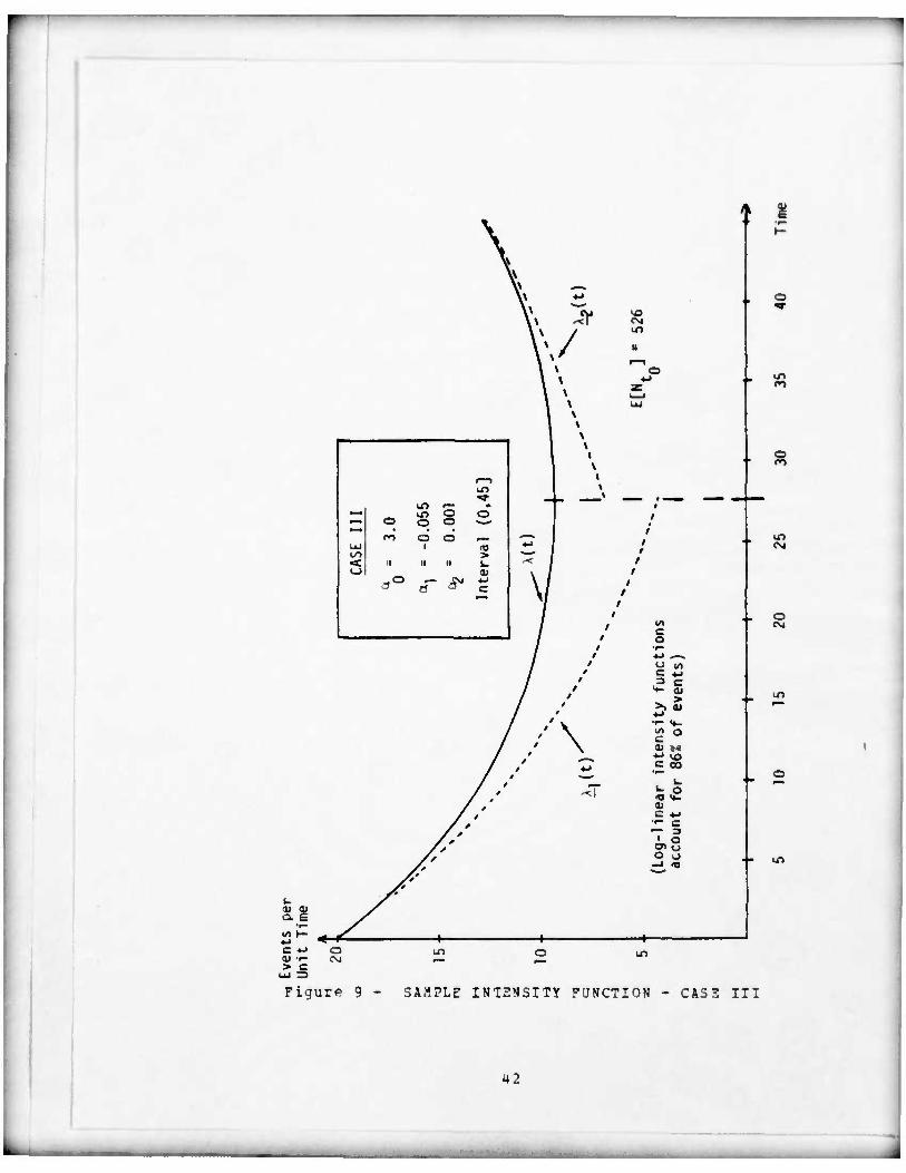
Figure 9 - SAMPLE INTENSITY FUNCTION - CA53 III

42

r—\ O uCt =» m m •-^ o o

*•• 8 - LU 00 o 1/1 • • • f—

<t r— o o <o <_) 1 1 > II II II

«3 o 1— CM c a a a ^*

;; o Ml

- o

CM 00

u Q

8.J

0> — > c

Figure 10 - SA.1PLS INTENSITY FUNCTION

o

o CM

. o

.

:.\SF iv

43

o

s CM

.* £>

.. o

r —« \ i

i—i o io

ro O o » CT> ro O to O o

LU • ^~ t/1 O O o ra < 1 > u k

II ii II

o F~ CM c a 3 a

*•> t/1 o *-> c c 3 1 o> \ —, >*

•-> <•- X ••» *• o

l/l

i . *<! C »4 \v 01 ^3

C \ \ •r- S_ \ \ O \ \ a \ \ V IA

C 4-> \ \ •«- c \ 1 <— 3

• o \ \ Ol (J

\ \ O U —1 <o

\ I ^•*

\ \ \ \ \ \ \ \ \\ \\ \i \\

o

O CM

.. o

&l </l I—

C -M oi •— > c

UJ =

<-+- -t- •f 00 VO TT CM

Figure 11 - SAMPLE INTENSITY PÖHCTI0S CASE V

44

I

1

i—i o *r (n *r —> CTl CVI 8 o » lO f— ~—

UJ o o o ^_ CO 1 <o «t > u II ii II

a CSJ *J a a a c

Pi Figure 12 - SAMPLE INTENSITY FUNCTION - CASE VI

L U5

IV. ALGORITHM IMPLEMENTATION

A. GENERAL

This section explains the several specific techniques

that were applied to implement the two competing algorithms

(Algorithm A and Algorithm 3) into FOBTRAN computer

programs. Detailed discussion of the various subprograms is

avoided since References 11 and 13 and attached program

listings provide such information. The Algorithms A and B

have some subprogram requirements in common while other

subprograms are unique to one algorithm or the other. This

section will discuss first those requirements common to both

algarithi£, then those needed only by the time-scale

transformation algorithm (Algorithm A) and finally those

unigue to the Poisson-decomposition and gap statistic

algorithm (Algorithm B). Hereafter differentiation b€tween

the algorithms and the FORTRAN computer program

implementation of the algorithms will not always be made.

The meaning will be clear from the context.

B. COMMCN REQUIREMENTS

1• Integration of a Degree-Two Exponential Pelvromial

Function over a Fixed Interval

Algorithm A requires that the intensity function

46

X (t) be integrated ever a fixed interval in order to

determine the value of the parameter of the Poisson random

variable that governs the number of events that are observed

to occur in the non-homogeneous Poisson process. Algorithm B

reguires that the intensity function X*(t) = X(t) - ^(t) ,

be integrated over a fixed interval for the same reason.

Since

b b b / A*(t)dt = / Mt)dt - / Mt)dt a a a

and \(t) has an explicit expression for its indefinite

integral, i.e.

/ \(t)dt = exp(YQ) exp(Y.t)

the problem for both algorithms is reduced to computing the

value for

/ X(t)dt = / exp(aQ + o^t + a2t ) dt

SUBROUTINE HELP employs IMSL FUNCTION HMDAW or the FORTRAN

supplied procedure DERF, as appropriate, to perform this

calculation. Section III-3 and Appendix B discuss how this

computation could also be made using a convergent series

representation.

2. Generation of a Poisson Variate with a Given

Parameter

Both candidate algorithms require at least one

realization on a Poisson distributed random variable with a

given parameter. The value assumed by the random variable

47

is the number of events observed in a specific interval of

tine over which the occurrence of events is governed by a

given intensity function (i.e. X (t) for Algoritha A and

X * (t) fcr Algoritha B) . The nature of most real event

streams which lend themselves to analysis using a

non-homogeneous Poisson process model is that they consist

of a large tctal number of events. This will be the case

either if a dense process is observed over an interval of

shcrt or moderate length or if a "sparse" process is

observed over an extended interval (see the arrivals at an

intensive care unit given in LEWIS [Ref. 9]). The point is

that both algorithms must be flexible enough to generate

ncn-homogeneous Poisscn processes that result in high

numbers cf events occurring. Since the number of events

occurring over any interval in such a process is a Poisson

random variable, it becomes necessary to be able to generate

a variate from a Poisson distribution with a large

parameter, i.e. large mean. The two most theoretically

straightforward algorithms for generating Poisson

distributed variates (the additive and multiplicative

methods) become computationally cumbersome as the parameter

of the random variable increases. Both the additive and

multiplicative algorithms and the practical deficiencies of

each are discussed in Appendix D.

The technigue selected to deliver a Poisson variate

on demand to both Algorithm A and Algorithem B is the Gamma

method. It is developed and explained in an unpublished

book by AHBENS and DIETER [Ref. 1], A paraphrased account

of the development of this algorithm is included in

Appendix E. The main advantage of AHRENS and OIETER's Gamma

method is that whereas the computer time reguired for the

additive and multiplicative methods is proportional to the

parameter of the Poisson distribution being sampled, the

computer time reguired by the Gamma method is proportional

to the logarithm of the parameter. The SUBROUTINE PVAR

48

^••••i^Bi^Hi^

employs the Gamma algorithm to return a Poisson variate when

given a parameter as an input.

3« I2§Q* Storage

Any algorithm which simulates a non-homogeneous

Poisson process must have some mechanism to provide the user

with information that completely describes the

realization (s) of the process simulated. Since the specific

arrangement of the stream of events over the interval is the

information cf interest to the analyst, the location, or

time of occurrence, of each single event on the interval

must be stored. Eguivalently, the spacings between events

would completely describe the realizations on a

ncn-homogenecus Poisson process. Thus event spacing

information rather than event location information could be

stored. (Programs written for candidate algorithms k and B

both provide the cption for the user tc demand either event

location or event spacing information.) «hen using either

algoritha, an array large enough to hold location or spacing

data for each event generated by the algorithm must be

created. Since the number of events observed in any

realization cf a non-homogeneous Poisson process is itself a

random variable, the precise size of the array cannot be

determined a priori. If the programs are to have any value

for general application, they must be able to accept

intensity function parameters which will demand large

numbers of events when simulated. Using the somewhat

arbitrary assumption that an event stream with an average of

4500 events is sufficient for most simulation scenarios, a

fixed array with a capacity for 5000 events is used in the

programs implementing both of the algorithms. If the value

of the intensity function integrated over the interval is as

high as the maximum limit of 4500 (i.e. the number of events

in the interval is Poisson distributed with mean = 4500)

49

—

then the array of length 5000 allows the Poisson random

variable to exceed its mean by 7.45 standard deviations

before an array overflow is encountered. This highly

unlikely event is of such rare occurrence (less than one

chance in a billion) that it «ay be disregarded. However,

should it cccur, the programs will reinitialize themselves

and generate a new Poisson process. Also an error indicator

is incremented. This error indicator (IER) «ay be written

on demand. Its value is the number of times the program was

forced tc abort generating a Poisson process, reinitialize

itself and start again.

A 5000 element array is small enough to avoid its

being an undue memory reguirement burden on most operating

systems, yet large enough to accommodate most

non-homogenecus Poisson processes of interest. Its choice,

though arbitrary, was based upon the above two

considerations.

C. SPECIAL REQUIREMENTS OP THE TIME-SCALE TRANSFORMATION

ALGORITHM (ALGORITHM A)

1• 5sif213 Variates

As explained in Section III-B, once the number of

events observed in the non-homogeneous Poisson process is established (i.e. N = n), it is necessary to construct a

tQ homogeneous Poisson process consisting of n events over an

interval cf length units. This is easily done by

generating n uniformly distributed variates on the interval

(0,1) and then scaling each by the factor u. The LLRANDOM

computer library package developed by LEWIS and LEARMONTH

[Ref. 12] is a very efficient source of such variates. Once

50

an array of n uniform (0,1) variat.es is obtained fro«

LLRANDOM, each element of the array must be multiplied by

the appropriate scaling factor. It is these resulting

numbers which must be acted upon by the inverse of the

integrated intensity function to yield the location of

events in the non-homogeneous Poisson process on the

original interval (0,tQ].

2 • Sorting of Events

Tc fce of much practical value a simulation routine

for a non-hcmogeneous Poisson process should order the

events in the interval from first to last. In Algorithm A,

this ordering may be done before applying the inverse

integrated intensity function to the elements in the

homogeneous Poisson process. The monotonic nature of the

integrated intensity function maintains the relative order

of all elements after they have been transformed by the

inverse function (see Figure 3). Of course the ordering

could be dene after the transformations also. In

inplementing Algorithm A, the uniform variates were scaled

by the factor '0 then ordered, from lowest to highest,

before being transformed by the inverse of the integrated

intensity function.

Ordering of large arrays of numbers is a time

consuming operation on the computer. There are many

ordering algorithms of varying degrees of sophistication and

efficiency. Because ordering is unavoidable when using

Algorithm A, selection of an efficient ordering routine is

important. The ordering algorithm used in this

implementation was the W. R. CHÖRCH computer center library

routine FXSOBT which employs Singleton's version of the

partition exchange sort. (A program listing of PXSCRT is

provided in the computer center's catalogue of library

51

-k. ...,.

routines.) The PXSORT routine appears to be the most

efficient ordering routine readily available for the

purpose. (It is acknowledged that «ore efficient routines

specifically tailored to the problem of ordering uniform

random variates may possibly have been developed that would

improve the overall efficiency of the program implementing

Algorithm A.)

3« Computation of the Transformed Values

The essence of Algorithm A is the application of the

inverse cf the integrated intensity function to each event

in the hoaogeneous Poisson process on the interval (C,yg].

As mentioned before, the intensity function, X(t), under

consideration does not yield an explicit expression for the

integrated intensity function, A(t) = ?(t), that must be

inverted. (Note: F(t) is a "scaled" distribution function).

Hence neither does a computationally convenient expression

for this inverse function exist. Numerical methods must be

employed to transform the position of each event on the

interval (0,Ug] in the homogeneous process tc its

corresponding position on the interval (0,tg] over which the

simulated non-homogeneous Poisson process is to be produced.

The Newton-Raphson technique was used to accomplish

the transformation. This technique allows for iterative

approximations which converge to the true transformed

.., tn; where ti = F_1(ui)) The (x.e. t1# t2. values.

iterati

for its corresponding t

iterations continue for each value u^ until an estimate t*

is found that satisfies

|F(t») - \ii I < e , where £ is a predeterained tolerance •5

level. (The specific value for used was x 10 • )

In the Newton-Raphson technique, given a function

h (x), the objective is to find the solution, x*, satisfying

52

• -.

the equation h (x*) • 0. Letting x^ be the initial estimate

for x* (based upon some reasonable criteria) the next

estimate for x*, that is, x 2» can be calculated fron the

fundamental iteration relationship,

h<V *k+l " xk h' (xk) '

This assumes that the function h(•) and its derivative h'(»)

can be evaluated at x^. The process is repeated k times

until |h (Xfc)| <e ; or, until |xk - xk+11 <e . This

procedure is nothing more than using the first two terms of

the Taylor series expansion of the function h(«) to locate

the x-intercept of the line tangent to h (x) at the point

h(xk). That intercept value becomes the next approximation

for the roct of h (x) and the procedure is repeated. A

graphical explanation of the Newton-Raphson method is

presented in Appendix E.

Applying the Newton-Raphson method to the present

problem requires some special modifications. The problem is

to find a value t. such that P(t.) = u., where u. is known,

i.e. to find t. = F (u.). Direct application of the

inverse F~ {•) is impossible since its functional form

defies all but the most abstract mathematical expression.

However if a new function G. (t) = F(t) - u. is defined and

if its root t*, determined (i.e. a t* such that G. (t*) = 0)

tL - F(t*) - au * 0, and P(t*) = a,. Thus t* = t* is the

value desired.

In order to apply the Newton-Raphson method tc the

function G . (t) it must be possible to calculate both G. (t)

and its derivative. Since G. (t) differs from F (t) only by a

constant, the problem reduces to that of evaluating F(t).

This has already been done, as previously explained in

Section III-E, and merely requires the assistance of

53

-

SÖEROOTINE BELP. Now G'^t) = F« (t), so talcing the

derivative cf G . (t) returns the intensity function \{t)

which is easily evaluated for any t. Clearly, the

Newton-Raphson method nay be used.

It shculd be noted here that for each u. there is a

corresponding function G.(t) on which the Newton-Raphson

technigue must be used. Since each use of the

Newton-Raphson method may require several iteraticns to

arrive at a value t* which satisfies the tolerance

criterion, it is readily evident that for large n,

considerable computational effort is required to obtain all

the values t. (i • 1, ...» n) . The number of iterations

required to arrive at a suitable approximation for each t.

is highly sensitive to the accuracy of the initial

approximation (designated t j if the initial approximation

is close to the actual t., the Newton-Raphson method will

converge very quickly. If the initial approximation is

poor, convergence could be much slower. The procedure used

to select initial approximations for each t. will therefore

have a profound effect upon the overall efficiency of

Algorithm A.

Selection cf these initial approximations is dene by

partitioning the interval (0,t ] into equal length segments.

The number of segments is equal to min[lO, n/t ]. The

function F(») is evaluated at the end points of each segment

and these end points, with their corresponding function

values are stored in an array. This procedure is performed

by SUBROUTINE BNCHMK. See Appendix E for a graphical

representation.

Io find an initial approximation for the t^ which

corresponds to any given u-, the array of function values is

searched until two adjacent function values which bracket u. J l are located. These adjacent function values uniquely

5«

identify the segment of the interval (0,t ] in which the

elusive t. is located. Either end point cf the segaent

would serve as a good initial approxiaation t* , f-r the

Newton-Raphson aethod. However, for the purpose of this

implementation, the end point which yielded the function

value closer to Uj_ is used for the initial approxiaaticn.

The decision to divide the interval (0,tQ] into

ain [10, n/U] segments was based upon eapirical results. Of

several proposed segaenting schemes that cne which resulted

in the fewest total nuaber of distribution function

evaluations over several intensity function/interval

scenarios was chosen. Higher values than n/u for sparse

event streams may produce better results. But n/4 gave good

results for dense streams and adequate results for sparse

streams. It appeared to be the best compromise as a

candidate for general usage. (The number of function

evaluations of G^(t) for each t^ averaged between 2.2 and

2.7 for this partitioning scheme.)

Alternative methods would be to use for the initial

approximation for t one of the following values:

Neither cf these other methods were attempted so it is

uncertain whether they would be more or less efficient than

the method which was used. Efficiency differences among the

three methods are probably not substantial since each will

usually yield a good first approximation.

55

awl

D. SPECIAL REQUIREMENTS 0? THE DECOMPOSITION ALGORITHM

(ALGORITHM B)

1. Intensity Function Categorization

The decomposition routine selected depends on which

of six possible shape categories the intensity function

\ (t) falls into (c.f. Figures 7 through 12) . An

examination cf the constants OLQ, a^ and ou in the intensity

function and the interval (0,tg] over which the

non-homogeneous poisson process is to occur will uniquely

identify the category of the intensity function. A thorough

discussion of this procedure is presented in Ref. 11, and is

net reproduced here. Implementation of the category

identification procedure requires a lengthy sequence of

decision statements within the computer program.

2« Selection of the Imbedded Loq-Li,near Intensity

f«SSlionJsi

Once the intensity function has been categorized it

must be decomposed in accordance with a complex scheme

described in Pef. 11. The objective of the decomposition

scheme is to fit a leg-linear curve (or curves) completely

underneath \ (t) on the interval (i.e. _\(t)< X (t) , 0<t<tQ)

in such a way as to laxiaize the area under the log-linear

curve (s) . This is done by partitioning of the interval

(0,tQ] into subintervals (0,b] and (b,tQ] if necessary, and

then by proper selection of the coefficients YQ and Y^ for

the log-linear function(s). These coefficients are

functions cf the coefficients a , i and » in the original

56

——

intensity function \ (t) and of the interval (0,tQ]. As the

program advances through the categorizing decision

statements, the proper coefficients are computed fcr the

appropriate leg-linear function(s).

3« £§E Statistics Algorithm

The precursor to L2WIS and SHEDLEB [Bef. 11] was a

paper by the same authors [Bef. 13] proposing a gap

statistics algorithm for simulating a non-homogeneous

Poisson process with a log-linear intensity function

X (s) = exp (ßQ • fh•)• (Beference 11 reviews this algorithm

in detail.) As previously noted, Algorithm B divides the

intensity function \(t) into a sum of two intensity

functions, X (t) and \*(t). The new intensity function

Mt) is chosen to take on the form of a log-linear function

so that the cap statistics algorithm may be used to generate

a stream of events from this portion of the original

intensity function X (t) . The S3BBO0TISE NHPP2 implements

the L2HIS and SHEDLEB gap statistics algorithm for the input

intensity function Mt) and returns an appropriate event

stream to the calling program. Since the use of the gap

statistics algorithm within Algorithm 3 is the rationale for

suspecting it to be a more efficient algorithm than the

time-scale transformation, it is instructive to examine the

efficiencies gained in using the gap statistics algorithm

vice a time-scale transformation algorithm on a leg-linear

intensity function. This question is addressed in Appendix

C. It was found that use of the gap statistics algorithm

resulted in a reduction in computer time of approxisately

50* from that required by the time-scale transformation

method.

57

MM

u• 2fee Be lection flouting

The gap statistics algorithm has efficiently produced an event stream from a non-homogeneous Poisson process defined by the log-linear intensity function

X (t) = exp(YQ • Yit)« Bat tBe process to be simulated has intensity function \ (t) * exp fa« • a-,t • a2t

2). It is therefore necessary to superpose an event stream frc» the intensity function

A*(t) = Mt] - X(t) 2

• expUQ + o^t + o2t ) - exp(YQ + Y^)

onto the event stream obtained fro« the log-linear intensity function.

Once it is determined how »any events are to occur over an interval with intensity function \*(t), i.e. H' • n', it is necessary tc select an ordered saaple of n' to variates from a distribution with density function

f*(t) = XMt)

/ u XMt)dt

The value n' will be saall compared to the total number of

events in the original non-homogeneous Poisson process.

Therefore the need for realizing efficiency in generating

these n' ordered variates is not usually as crucial to

overall algorithm performance as is the need for efficiency

in producing the non-homogeneous Poisson process fro» the

log-linear intensity, \(t), in Step 3. However if the

technique for obtaining these n' ordered variates is

58

•i

extremely inefficient, auch or all of the efficiency gains

realized frca Step 3 above cculd be lost here. (In fact an

example of such a loss of previously gained efficiency is

documented in this thesis; see Section VI-B.)

The rejection «ethcd is particulary useful for

generating randoa variates froa populations with continuous

densities that are bounded and which are concentrated on a

finite interval; this is the case for f*(t). The rejection

aethod and an algoritha for its iapleaentaticn are presented

in LEWIS and SHEDLER [Ref. 11]. A geoaetric arguaent will

suffice to exhibit the principle involved. Consider the

density function f (x), for a randoa variable X on the

interval (a,b) in Pigure 13. The aaxiaua ordinate of this

density is c. If another function g (x) * c* > c is

constructed then the density function f(x) is enclosed

within the rectangle (a,0) , (b,0), (a,c*), (b,c*) . If a

point within this rectangle is selected at randoa it will

fall either under the density function or above it. If it

is under the density curve the abscissa of that point is

accepted as a variate from the population. If the point

lies above the density curve that point is rejected and

another point within the rectangle is selected at randoa.

The procedure continues until n' variates have been

produced. The random points within the rectangle are easily

produced ty generating two independent uniform (0,1)

variates and scaling them properly resulting in a point

(x,y), where x = a • u,(b - a) and y = u2»c*. Then if

f(x) > y, x is accepted as a variate, otherwise it is not.

After n* variates have been obtained, they are ordered to

yield an event stream for a process with intensity function

X*(t). S0EROOTINE REJECT employs this method in the

program far Algorithm B.

59

- --•

* X

The density f(x) is comDletely enclosed by the rectangle

(a,0), (b,0), (a,c*), (b,c*).

Procedure:

1. Generate 2 ''ndepende-r; jniform (0,1] variates u,

and u~.

2. Compute: x = a + bu , y = ;*u?.

3. Plot (x,y).

«. If the point (x,y) lies under the density f(x) accept x

as a /ariate; otherwise go to Step 1.

Example: In the graphical example above x, would be accepted

as a variate whereas x? would not be accepted.

(Note: Ideally, c* = c and a and b correspond

to the lateral limits of the density f(x). This

minimizes '•ejection region.)

Figure 13 - THE REJECTION-ACCEPTANCE METHOD 0? 7A3IATE

GENERATION PBOfl AN ARBITRARY DENSITY

60

I -- -- • -

_ —

Since the probability that a point on the abscissa

will not te accepted as a variate is proportional tc the

area within the rectangle that is not under the density

function, it is advantageous to make this area as snail as

possible. Therefore it is best to set c* = c and set the

values a and b equal to the end points of the interval over

which the density function occurs. This is desirable but

not necessary. Pigure 13 illustrates the «ore general case

where the rectangle is larger than necessary. One »ay be

required to select a c* > c if c is difficult to determine.

Seldom would a and b not coincide with the lateral limits of

the density however.

It is obvious from Figure 13 and the preceding

discussion of the rejection method of variate generation

that it is the "shape" of the density function which is

critical to the validity of the method and not the fact that

it integrates to one. Therefore any scaled density would

preserve the relative shape of the density function. As

long as the value c* is at least as great as the maximum

value of the scaled density, the rejection method will yield

valid variates. The intensity function \*(t) may be thought

of as a density scaled by the factor u* = / °x*(t)dt. 0 0

Algorithm B uses the intensity function X*(t) rather than

the density function \*(t)/u« in the rejection routine.

This eliminates a division step for every function

evaluation required by the method.

5« 5iEaJ23 SvenE Streams

The event streams from the intensity functions X (t)

and A*(t) must be merged to produce an event stream from

X (t) = x(t) • x *(t) . In the present case there are two

event streams (one long and one short) which are already

61

•H ~- ^_ _~.

ordered. This structure allows for superposition rather

than a more general (and mere time consuming) ordering

procedure. To do this merging job SUBROUTINE COLATE is

called.

E. SUMMARY

This section has presented a general discussion of the

more significant and interesting procedures used to

implement Algorithms A and B efficiently in FORTSAH. The

reader is referred to LEWIS and SCHEDLEH [Ref. 11] for a

detailed listing of steps for Algorithm B. Program listings

may also te consulted. These may be found after Appendix E.

62

- - - - ._ ._.__

METHOD OF COMPARISON OF ALGORITHMS

GENEHAL

Conclusions drawn from the results of comparing the

efficiencies of two computer programs are only as sound as

the measures of effectiveness upon which they are tased.

These measures of effectiveness are always somewhat

arbitrary, so their selection should be based upon

compelling reasoning.

Even after reasonable methods of effectiveness have been

defined, only a finite number of trials (usually a small

finite number) for a given set of circumstances may be run.

Therefore, general statements such as "this algorithm is

better than that algorithm" can seldom be made with complete

confidence. Yet if the incomplete information gathered

reveals certain trends, generalizations hypothesized from

such trends may warrant a high degree of confidence.

This section describes how the two algorithms are

compared and the rationale for choosing the method employed.

63

B. HEASUEES OF EFFECTIVENESS

1. CCBPUtational Speed

Perhaps the most popular efficiency measure for

computer programs is their speed of execution. Speed is a

natural standard as long as computer time remains a costly,

scarce resource.

Algorithms A and B were compared in terms cf the

mean time required to generate event streams from a given

set of intensity functions. It should be noted that since

the number of events in each event stream is a random

variable, the time required to generate one event stream is

also a random variable.

Several event streams with different intensity

functions, each having a different expected number of

events, are produced. Event streams for each of these

intensity functions are replicated many times by each

algorithm. The total execution time required for all

replications is the "speed" measure of effectiveness.

The number of replications varies with each

intensity function. For example, an event stream with an

expected number of events less than 200 was replicated 100

tiies whereas event streams with over 1000 expected events

were replicated only 30 times. In both cases the total

number cf events produced was of the same order of

magnitude. A priori it seemed reasonable to assume that

computer time required to execute each algorithm's program

would be roughly proportional to the total number of events

6U

û

generated. Therefore in designing the experiment the

product of the expected nuaber of events tiaes the nuaber of

replications (E[Nt ] x # reps) was kept roughly constant in

order to keep deaands on coaputer tiae reasonably under

control. (Note: Prograa execution tiaes were isolated froa

coapilaticn and linkage tiaes for the purpose of the

computational speed coaparison.)

2. Coaguter Memory Requireaents

k second natural efficiency measure for coaputer

prcgraas is their core memory requirement. Both prcgraas

were written with the goal in aind of conserving as auch

memory as possible without unduly increasing prograa

complexity. Cere requireaents reductions could aost likely

be accomplished in both prograas through more sophisticated

programming methods. Therefore this comparison has a major

weakness as a measure of effectiveness. Recognizing this

caveat, memory requirements for each prograa were coapared.

3. Fidelity,

The question of paramount importance is: How well

does the program simulate the true process? This is a

difficult question to answer when dealing with a finite

number of realizations on a process whose theoretical

properties can be validated only after an infinite number of

realizations.

Several aethods of comparison are possible. The

simplest is that cf comparing the sample means and sample

variances of the random variable whose realizations are the

number of events generated on an interval by a given

intensity function. This random variable should be Pcisson

65

—

distributed with mean equal to the integral of the intensity

function over the interval. For a Poisson rando» variable,

the variance equals the mean. This test, although useful

for determining if either algorithm varies grossly fro«

expected performance, yields no information about he« the

algorithms are distributing their simulated events over the

interval. It is necessary to look at discrete segments of

the interval and examine the distribution of the number of

events produced in each segment by our simulated

non-homogenecus Poisson process.

From the definition of a non-homogeneous Poisson

process (see Section II-B) we know that the number of events

observed over any segment of the interval must be a Poisson

random variable with parameter equal to the integral of the

intensity function evaluated over the interval. 3y dividing

into several segments the interval over which the Pcisson

process is being simulated, the number of events in each

segment can be observed. Two hypothesis tests may then be

made for each segment.

The first test is the dispersion test [Eef. 3,

p. 158]. This test seeks to ascertain if the number of

events observed over each segment is distributed as a

Poisson random variable, Let n , n2. n, be k k observations on the number N of events occurring in a given

P_ fixed segment p, and let n = (n, • ...•n. )/k. If M is a r pi k p Poisson distributed random variable, then the statistic

j • . (n . -n = JL±Z1 Eli E

- ,2

has a distribution which is approximated by a chi-sguared

distribution with k - 1 degrees of freedom. If the interval

has been partitioned into m segments, then by simulating the

ncn-homogeneous Poisson process k times, we can perform m

66

hypothesis tests at a selected significance level a . The

test statistic d would then be compared to the (1-o)

percentile of the chi-squared distribution with k - 1

degrees cf freedom. For a large number of hypothesis tests,

say 1000, we would expect approximately 1000a rejections of

the null hypothesis, if in fact the N 's are Poisson P

distributed.

Fcr example consider the non-homogeneous Poisson

process over the interval (0,100]. If this interval were

partitioned into 100 unit segments the number of events

occurring in each segment should be Poisson distributed. If

51 event streams are simulated over the interval, a value

for the test statistic d may be computed for each segment,

i.e.

) i , n .-n ) d = 1=1 P'1 ?

P

Assuming a significance level a= .05 and comparing each d 2 P to the critical value v_„ = 67.50U8, we would count the A50,a

number cf test statistics such that d„ > 67.5048. If the P

number of events in the segments are indeed Poisson random

variables we would expect, on the average, that 5 out cf the

100 dp values would exceed the critical value.

In the above discussion of the dispersion test, no

mention was made of the parameters of the Poisson random

variables (assuming that they are Poisson). This is because

the dispersion test for Poisson distributions is parameter

independent. Thus it is necessary to perform a second

hypothesis test to determine if the mean number of events

per segment is equal to the difference of the integrated

intensity function evaluated it the right and left end

points of the segment respectively. For large k the sample

mean n is normally distributed. Under the null hypothesis,

67

i.e. that the aean of Np •/ JA(t)dt »uD («here a. and a. are

the end feints of segment p) n is normally distributed with

mean np and variance Mr/** The test statistic is

. . & - V

and the critical value is the 0~y ) percentile of the

normal distribution, za/2« Again, there would be one

hypothesis test for each segment and if we made 1000 such

tests we would expect to reject the cull hypothesis

approximately 1000a times, on the average.

Continuing the example above, it is now of interest

to see if the mean number of events on each segment agrees

with the theoretical value determined by the integrated

intensity function. This time assuming a significance level

of a • .10, the critical value for each test statistic Cp

would be zw2=1,6a5* Each c > 1.6U5 would be counted and

if in fact the random variables have the hypothesized means,

we would expect (on the average) that approximately 10 test

statistics cut of 100 would exceed 1.6U5.

After the dispersion test and hypothesis test for

the means have been performed on event streams from each

algorithm, the test results may be compared to see if either

algorithm appears to have null hypothesis rejection

percentages which are not consistent with the i levels of

the hypothesis tests.

(It should be noted that during the development of

the programs histograms of the event streams were plotted to

determine whether or not they "fit" their respective

intensity functions. Both programs seemed to produce

satisfactory results by this subjective measure.)

68

__

C. OTHER CONSIDERATIONS

1 • ISiSüJÜI IüH£li2ü Category

Algorithm B classifies the input intensity function

into one of six categories and then determines what action

to take tc generate the appropriate event stream. It might

be expected that the speed of Algorithm B will be affected

not only by the total number of events to be generated but

also by the form of the input intensity function.

Decomposition of the intensity function into four sections

will prctably reguire more time than if it must be divided

into just tMO sections.

Algorithm A treats all intensity functions alike.

Therefore, it is important to compare the two algorithms for

all six possible categories of intensity functions. It is

possible that Algorithm B could be faster than Algorithm A

for one category of intensity function and slower than

Algorithm A fcr a different category of intensity function.

The six intensity functions selected for the comparison

represent all of the categories defined by Algorithm B, and

are, in fact, these intensity functions illustrated in

Pigures 7 through 12 of Section III. These categories are

numbered frcin I through VI and correspond directly to those

listed in Ref. 11.

2• Evaluation of c« Value in R£iection Routine

The importance of reducing the size of the rectangle

enclosing the intensity function ,\*(t) prior to beginning

the rejection algorithm was mentioned in Section IV-D. If

possible c* should correspond to the maximum value of \*(t)

69

on the interval (0,t ]. For Cases I and II (Figures 7 and 8)

this maximum value is easily determined since it occurs at

one of the end points of the interval. For Case III (Figure

9) the maximum values of \ * (t) and x£(t) both occur at the

point b «here the interval (0,tQ ] has been partitioned into

two subintervals (0,b] and (b,t ]. For Cases IV, V and VI,

(Figures 10, 11 and 12) the maximum value of \*(t) is not so

easily determined. LEWIS and SHEDL2R [Ref. 11, p. 11] state

that it is not possible to find this maximum explicitly.

However an upper bound may be determined from the values k

and k where \{t) < k and \ (t) > k on the interval (0,tQ ] (or

subintervals (0,b] and (b,tQ ] for Case VI). Then by setting

c* = k - k it is certain that \*(t) < c* on the interval or

sutintervals cf interest. Figure 14 which illustrates the

rejection routine for the intensity functions for Case V and

VI used in the analysis, reveals that the c* computed in

such a manner »ay not be very efficient as an upper bound

for the rejection algorithm. One would expect some

reduction in speed efficiency for Algorithm 3 when c*

greatly exceeds the maximum value of \*(t).

3• Designated Tolerance Level

Algorithm A reguires selection of a tolerance level

which determines the stopping criterion for Newton-Raphson

iterations. The speed of the algorithm could be expected tc

be very sensitive to this tolerance limit. By setting it

too small the comparison would be prejudiced in favor of

Algorithm B. By not setting it small enough the fidelity of

the resulting event stream to the true intensity function

would be impaired.

CNtQ] x 10

It was -7

determined that a tolerance level of

occasionally demanded that the cosputer

discriminate beyond its significant digit capability in

70

Single precision. This resulted in the failure of the

Newton-Raphson iterations to converge, although in theory

they would have done so if enough precision had been

retained. A tolerance level of B[N ] x 10~ seeaed to be 0

unnecessanl" deaanding on Algorithm A even though the

computer couxd discriminate at this level. A stopping rule

fixing C • 2[Nfc ] x 10 ' was the coaproaise that insured

reasonable accuracy of the simulated event streaa without

unfairly burdening Algorithm A.

71

^„__

5

4 -

2 --

(Acceptance region accounts for less than 4$ of the total area in the rectangle.)

max A*(t) * 0.3

•\*(t)

10 20 30

Figure 14a - Graph of Rejection Routine for the Case V

Intensity Function Analyzed

c| = 4.92

4 •-

2 -.

c* = 2.92

max X*(t) ± 1.7

Figure 14b - Graph of Rejection Routines for the Case VI

Intensity Function Analyzed

Figur? 14 - ILLUSTRATION OF REJECTION-ACCEPTANCE REGIONS

FOR SAMPLE CASE V AND CASE 71 INTENSITY F'JNCTIO'IS

72

.... uotfl • - -

71. RESULTS AND £ONCLJSICNS

A. GENERAL

Coaputer prograas impleaenting Algorithas A and E were

ccapared in teras of efficiency as explained in Section V.

This section docuaents the results of the coapariscn and

discusses general observations of the author concerning the

tue competing prograas. Also recoaaendations for further

study concerning Algorithn B are offered.

8. XEkSUBES OP EFFECTIVENESS RESULTS

1. Sêe d

Table I convincingly illustrates the superiority of

Algorithn B over Algorithn A when coaputational speed is

used as a measure of effectiveness. The column in Tatle I

labeled "Time A/Tiae B" is the ratio of the total tiae

reguired by Algoritha A to produce a specified nuaber of

replications of the given non-homogeneous Poisson process,

to the tiae required by Algorithm 3 to produce the saae

number of replications of the process. For all six

representative intensity functions the Pcisscn-decoaposition

and gap statistic algoritha is at least twice as fast as the

time-scale transformation. For large event streams the

superiority cf Algoritha B is even more pronounced.

73

••I tMimi

r Table I - COMPUTATION TIMES FOR EVENT STREAMS

<IBM System 360/67, FORTRAN IV (G) compiler)

,» .M

•0SJ • «ft « I «A

co « fl •1 *<

%• ff 55 W 3 5"

•*- x o 41 — w • •••- «/» — 3 «1 ••• tfj %. 'ZZ *ts 5i| *i • vi 01 w O «•w *-J y " 3 > 3 5X3 t > E

•n — - • _a e o c « _.

€ • 41 O «1

VI z$i xê M

«1 VI C

3 -2c «gu •o 2 o V» o <*- •- C O M

CM — *J its <M — —

9 D t°a 12 — V (M f W V» 4" » y C y AJ — U i

Ct. — L. M D .- «I x-ü *- i a a ** «^^ •*•» 4-*

• VI VI M u -> 3 M *•» «i -* —• —• *-» —' Ov"

-raw ^— l_ re « « « « * u « « «•> c -»*. <-< -< -< *«w -«: -< - ' *- •a «l e o «S O «*> o — • > o X x X X K O X X

a*-« IS i- 2 IS 88«, ass w u 3 u 3 vi 3

•J k VI • • • 41 A « A • s A «a HI « e*i • S 4-» M n OJ 0» • «1 « • 00 « • •* • * -TT

CO O T» E UN J u u u •— II u ^ ü ytN

«I ^ -^ i «cm r o 9« ° m in ^ ^ — m 1 »t» 9 CM CM 00 U> P- 1 -. | -F r^ u-> n CM «n CM VO CM en } »~lf- ~ ~ i

i . . « c T? i » • •» • — 5 y l 1 <M

— H 9 u-) i o Qi i** — i *n 09> in 10 101 • CVJ »• mo 1 « «-> • W 3"^ — 1 CM CM GO Oil en <oi io en oo> cn r^ 001 — CJ» 1 O U • Ol I •— CM •— <ni — »«>—«-'

1 ' 1 1 X -~ i

1 -u I— 1

i

CM z eo i m ~- i in sis IMI 00

en» »n mi 3 •1 r» «i ro

1 1 mi oo in> o

H o i <o CMl ^

»i « CM" CM -; a

o lO i «a

1 ~l o C\|l CM cgi CM

tni m ^ i r<K si s *• •

<Mi ru M * ' » 1

urt i in <MI nj

1 1 1 1

B 1 1

k < 1 00 <Z i CO <l 00 <•' oa <| oo <| CO O 1 Ol 1

1 «« • VI ft O

m a in s s 8 •" ^

f^ » <M M ^ s * o vO CM r*. CM «I * <o m CM

z t__i Ui

UJ

8 >• > = V

e

S B

I

S c

I VI w

VI

cS

7a

The most obvious disparity revealed in Table I is

the difference in speed efficiency (of Algorithm E with

respect to Algorithm A) between the group of Cases I, II and

III; and the group of Cases IV, V and 71. In the fcraer

group Algorithm B was 5 to 7.6 tines as fast as Algorithm A.

Per the latter group Algoritha B was only 2.2 to 2.5 tines

as fast as Algoritha A.

This difference between the two groups immediately

nade suspect the value c* used in the rejection routine of

Algorithm B. Por the first group c* is set at the least

upper bound for \* (t) . For the second group c* is not, in

general, a least upper bound for **(t) but is only an upper

bcund. To determine whether or not this difference in the

"quality" of the c* values could have such an adverse effect

on time efficiency for Cases IV, V and VI, these cases were

simulated a second time with new c* values which were

empirically evaluated by graphical methods. These modified

c* values were set close to the least upper bounds of the

respective \*(t) component of the intensity functions for

each case. Marked time efficiency gains were observed (see

Discussicn column, Table I) indicating that significant

efficiency losse~ can be sustained due to the method of

setting c* values in Cases IV, V and IT. «

Three factors appear to influence the degree of

speed efficiency gains of Algoritha B over Algoritha A.

First is the selection of the c* value as discussed above.

The second factor is the percentage of total events which

Algoritha E must generate from the rejection routine. For

the specific intensity functions analyzed, this percentage

ranged from U% in Case V to 2U% in Case VI. The fewer

events required from the rejection algoritha relative to the

number generated from the gap statistics algoritha, the

greater the efficiency of Algoritha 3.

75

Finally the total number of events in an event

streaa affects relative efficiencies between Algorithms A

and B. This is because as the number of events to be sorted

by Algorithm A grows, the less efficient its sorting routine

becomes. Sorting requirements for Algorithm B are greatly

reduced due to the properties of the gap statistic procedure

used. Therefore as total events increase, so does the

efficiency advantage of Algorithm B over Algorithm A

increase.

2. Computer Memory Requirements

Algorithm A requires approximately 72,000 bytes of

core storage. Algorithm 3 demands about 92,000 bytes. Both

programs are costly in terms of storage due to the number of

library routines used and the need to store up to 5000 event

times. The difference of 20,000 bytes would not be

important unless computer capacity were being challenged.

Memory requirements for both algorithms could be reduced by

reducing the event stream capacity of the programs. A

reduction of capacity from a maximum of 5000 events to a

maximum cf 2000 events in each program would result in

storage requirements of 54,000 bytes and 68,000 bytes for

Algorithm A and Algorithm B respectively.

3. Fidelity.

Table II lists the results of six series of

hypothesis tests of the types discussed in Section V-B.

Three series of dispersion tests and three series of

hypothesis tests for the mean were conducted. Intensity

functions for Cases III, 17 and VI were selected fcr these

tests.

76

Per each of the three cases, a large number (500,

900 or 1000) of each type of hypothesis test was performed

for a fixed level of significance a. The number of tiaes

each null hypothesis was rejected was recorded and the

statistic 0 • [(nuaber of rejections)/(total tests)} was

computed for the series of dispersion tests and the series

of hypothesis tests for the aean. If the null hypothesis is

true, then a is an estiaate of the significance level a.

Froa Table II it appears that for the hypotheses

tests associated with Case III and Case IV, a gives a very

good estiaate for a, the true significance level. Por Case

VI some disparities are observed. For Algoritha B the a

value for the dispersion test (i.e. hypothesis test that

variates are Poisson distributed) is 0.039 whereas the

significance level is ot • 0.01. Algorithm A yields a much

better a value of 0.012. Por the hypothesis tests for the

aean, both Algorithm A and 3 yield a values almost twice

that of a •

These results, though interesting, are inconclusive.

Por the dispersion test, the statistic

d = Lx=1 P'1 P P D

P

is only approximately distributed as a chi-sguared randoa

variable. It has been shown by FISHER [3ef. 4] that for

Poisson random variables with low expectations, hypothesis

tests based on the chi-sguared distribution may produce

spurious results. Also, we would expect that if the

distribution of d is only approximated by the chi-sguared p

distribution, that the relative error between the

approximate and true distribution is greatest in the tails,

i.e. at high percentile values. Case VI was tested at an a

level cf 0.01. It is also the intensity function with the

77

•

fewest expected number of events of the three intensity

functions tested. Partitioning of the interval into

segments produced some segments which had a low expected

number of events (see the right tail of the density function

pictured in Figure 12). The results for Case VI rather than

indicating any serious flaws in either of the algorithms

suggest further research into finding better ways of

hypothesis testing for sparse event streams and highly

discriminating levels of significance.

Kesults of the hypotheses tests on Cases III and IV

indicate that both algorithms simulate event streams that

ccnfora to the desired hon-homogeneous Poisscn processes.

78

• i in — ^

1

Table II - RESULTS OP HYPOTHESES TESTS FOR FIDELITY

(IBM System 360/67, FORTRAN IV (G) coapilar)

M 1 -t H 4-* 1 Q. 1 u Q. 1 u 1 01 O i 01 o 01 O • V o u x • "i x J X I •o X y I 0) 1 w * Of < 1 cc < QC

| 1^

o » i/l

<*i 1 !••» o § o H ®

4* «t • Ol > l/l •o • •

X a.

a 3 S <e <a M i 4-1 4-1

TJ •o g 1_ o IT) 'O 4-* > o 00 i» o i o ^ O* p^ *<

01 • i/l 9 1 u-1 <•* o ••1 V» * • •

V» «o ••- "O a *—%m <_> W <a <a

Wl h- V £

ii

4-1 c i 9 1 s O

O O a*

co 1 .-sj S 9 <M s I */» ^ 1 ol W

01 • »— CO co l/l m i • •Q 3 o w 18

1

<a

i

| Cvl en

o i»»

• > i/» s cu O

if en o

E 01 M en en <c

T3 l/l •a O

<o 1 M

M • o fa < a 1 <0 41 m ^ 0 3 H M

0 § > M IT) U-» 1 ao

o > O

l/l 1 U1 i eg

i o •a i " VI c 01 H *— V »

o l/l •D • 1 N «A l/l •a a Of l/l <J L- < a I <3 .C t— 4-1 o

o

s X* o Cn

1 o i K>

i S — S 1 \o t <— ^ « l/l O I en

01 • 0— 00 CO l/l •O N 1 i fl a O

1— I ' 3 » <a

/uuo^sueJX ' \ / UO ijisoduio3aa\

va(»3S-9uiii- 1 I UOSSlOd / v wHiiaosiv a HHJ.IH09TV

7P

___

C. GENERAL OBSERVATIONS

1• Programming Ease

The programming of Algorithm A is simpler than the

programming of Algroithm 3. Because the time-scale

transformation technique handles all intensity functions

alike, several different cases need not be identified.

Algorithm B must categorize the input intensity function

into one of six categories and then must treat each category

in a unique way. A rough indication of this difference in

the degree cf complexity is the number of instruction

statements required by each program. The program

implementing Algorithm A required 142 instructions. The

program fcr Algorithm B required 364 instructions.

2« Exact Bet hod Versus Agprpximate Method

Algorithm B employs an exact method in generating

the non-hcmogeneous Poisson event stream. It is exact in

the sense that all event times are calculated directly and

the precision of those calculations are limited only by the

physical constraints of the computer.

Algoritha A employs a Newton-Raphson iterative

method tc approximate event times on the interval. The

stepping criterion for the technique is limited by machine

precision considerations. Also the stopping rule does not

give a firm account of the magnitude of error that can be

expected in the event times. The epsilcn criterion is

applied tc the value of the integrated intensity function

80

and not to the abscissa, (or time interval axis). Por the

integrated intensity function, ?(t), it is conjectured that

given a function value Fft^) = u^, if a t = t1 can be found

such that |P(t«) - Fftjjl < t that t' is very close to t ^

although this is a reasonable assumption given the

well-behaved nature of the integrated intensity function,

the problem of not knowing how close t' is to t* may tend to

reduce one's confidence in the algorithm.

3« Initialization

The initialization time required for the programs

implementing the two algorithms has not yet been mentioned.

Computation time comparisons did not include compilation or

linkage times required for the two algorithms. These

initialization times were significantly different, being

approximatelj 16 seconds for Algorithm B and only 8 seconds

for Algorithm A. Should simulation of only one or two event

streams be required it is likely that Algorithm A may

actually require less total time than Algorithm B. The

difference between the initialization times could probably

be reduced if the programs were to be rewritten in Assembler

language.

D. CONCLUSION AND RECCMH2NDATIONS

1. Conclusion

For general usage, the Poissor.-decompositior and gap statistic method of LEWIS and SHSDLER [Ref. 11] is clearly superior to the time-scale transformation method in generating a non-homogeneous Poisson process with a

31

degree-twc exponential polynomial intensity function.

The main advantages of the Poisson-decomposition and

gap statistic algorithm are its speed and its qualification

as an exact nethod of variate generation.

The time-scale transformation method enjoys some

advantage in core storage requirements and in lower program

initialization time. These advantages are not sufficient to

overcome the relative deficiencies of much greater

computation time and uncertainty about the accuracy of the

approximating mechanism for determining event times.

2• Recommendations

The full potential of the Poisson-decomposition and

gap statistic algorithm can not be realized until it

includes a better method for selecting an upper limit value

c* for Cases IV, 7 and VI intensity functions. Algorithms

for choosing a c* value that will be close to the laxiaum

value for the function ,\ * (t) should be developed and

incorporated into Algorithm B. A single variable search

technique (such as a Golden Section search or Bisection

search) for finding the maxinum value of a unimodal function

may be appropriate.

The computer program for Algorithm B should be

rewritten in Assembler language in order tc reduce program

initialization time. The program could then be developed

into a library routine for general use.

The question of fidelity of the simulated

ncn-homogenecus Poisson process to the true theoretical

process should be investigated further. Of special interest

is the question of how well the algoritha simulates sparse

82

event streaas. Methods for conducting the dispersion test

and the hypothesis test for the aean at very high levels of

significance (i.e. a = .01, .005) for intervals with a low

mean number of events are needed.

83

APPENDIX 1

PHOOF OP THE VALIDITY OF SCALING THE INVERSE DISTRIEOTION

FUNCTION

Proposition: Let T be a continuous random variable with

distribution function F (•) , such that T

FT(t) = 0

FT(t) = A(t) - A(0) o < t < t0

FT(t) = 1 t > t,

Let Y = M F (T) such that T € f0»1,,) and is a real number.

Then the random variable Y is uniformly distributed en the

interval 10.UJ . 0

Proof; F {•) maps the line segment [0,t ] onto the interval

[0,1]. If F (•) is strictly increasing on (0»t0) then

F"1 (•) exists on the interval (0,1) and maps (0,1) cnto

(0,tQ). Now,

Fy(y) = P[Y < y] = P[UQFT(T) < y]

= P[F_(T) -*-)]

= P[T < F~X(-*-) ] -1

i *T

= F {F"1^)} T T UQ

FY(y) * -*- Y Wn 0 < y < u,

84

m • • h.».»..

Therefore,

dFy(y) fY(y) - ;* 0 < y < u.

and Y is uniformly distributed on the interval (0, Ug)

85

• •--

APPENDIX B

E3R0H PUNCTICN AHD DAMSON'S INTEGaAL HEPBESENTATION CP THE

INTEGRATED INTENSITI FUNCTION A (t)

The standard for« for the error function is:

0 t 2 2 e -u —- / e du . /if 0

Dawson's integral is usually represented as:

t 2 t"2 / eu du .

0

Both of these integrals «ay be calculated to any d«sired

degree cf accuracy by using the exponential series

expansion,

a> n X r X

• • ) —r n=0

2 2 u -u Thus, e and e aay be written as

2 • , 2, n °° 2n PU _ Y (u ) _ v H_

_'- El A« n! n=0 n=0 ,!

86

and

,-u2 . y (-u2)n y (-i)n(u2n) n=0 n=0

respectively. Integrating eu yields

t 2 t - u2n / eu du = / y —p- du 0 0 n=0 n-

" t 2n

n=0 0 n#

a. 2n+l = L (2n+l)n! n=0

-2 Multiplyirg by t results in

2 t u2 » fc2n-l

' { e du " Jo ^^

and the series representation for Dawson's integral is

revealed. This series will converge for all t, althouch the

value of the integral increases very rapidly as t increases.

87

-y" --^-

Using the saie argument it is easily shown that the /•t -u2 representation for /,, e du is

series

I <-l)n t2n+1 n-0 (2n+l)n!

The error function is obtained by multiplying the integral

by the constant 2//rr »i.e..

t 2 -2- / e"u du Sn 0

(-1)" t2n+1

/? n-0 '

Although the series expansion nay be used to calculate both

functions, there are very efficient computer library routines available for coaputing Dawson's integral and the

error function.

The FORTRAN supplied procedures EEP and DERP [Ref. 15]

evaluate the above function for input values of t.

The IHSL (International Mathematical and Statistical Libraries, Inc.) FUNCTION MMDAtf [Ref. 6] evaluates Dawson's integral for input values of t.

It remains to be shown that the intensity functior 2

,\ (t) = exp{a, * out • oi_t } may be integrated over tue

interval (0,t ] using either ERF (or DER7) or IBOAI.

88

• - - -

Consider,

MO-A(O) • / X(t)dt = / exp(an + a. t + a,t )dt 0 0 u L 2

By completing the sguare of the exponent the expression

becomes

A(tQ) = /to exp jaQ - îj exp | a2(t + ^)J dt

( A(0) • 0# since 0 is the left end point of the interval

over which \ (t) is defined) .

For a_> 0,

A(tQ) = exp aQ '0 | r- ,. ai '2

4a 2 ) 0 / u exp { /ST (t + -~)| dt 2a.

Letting, «1, U = /ÖT (t + T5 )

2 2a 2

du = /al dt

K' = exp {* - 0 4a.

and adjusting the limits of integration, the expression becomes:

A(tQ) = ; / e du = < / e du - / e du? /a. a /a- ( 0 o J

89

«here,

and

a =

b =

<•*? IE

S> {C0 * 2^)

The expression above can be rewritten as follows:

A(tQ) = _K_

fir. {bV2 /b eu2du - a2a"2 [

0 0 S du)

Inside the brackets are two Dawson integral expressions

multiplied by constants. Outside the brackets is just one

more easily determined constant. Using .I.IDAW twice and

multiplying by the appropriate constants will give the

desired integral value.

For a. < 0,

A(tn) = exp { a. exp -|a2! (t + •VI 2a2 ) dt

exP ao " 4^7 \ L exP «1, 2

- f^T^T (t •a**] dt

Substituting as before gives

A(tQ) K

/fa

K

/To

b _ 2 / e~u du a

•i ( /?

/ e du - ~> a

"F" ' e /? 0 •u2 du]

90

•-• - -

1

and the error function can be recognized within the

brackets.

Two error function calculations, a subtraction aod a

multiplication by a constant are sufficient to determine

A(t ). o

91

MM

APPENDIX C

COMPARISON OP GAP STATISTICS ALGORITHM AMD TIME-SCALE

TRANSPOHMATICN ALGORITHM POR SIMULATION OF NON-HOMOGENEOUS

POISSON PROCESSES WITH LOG-LINEAR INTENSITY FUNCTIONS

LEWIS and SHEDLSR [Ref. 13] present two algorithms

for simulation of non-homogeneous Poisson processes with

intensity function X(t) = exp(ß *ß t) . The first algorithm,

which uses a time-scale transformation is easy to employ

since the inverse of the integrated intensity function is

known explicity. The second algorithm uses gap statistics

to generate event streams.

Ecth methods are exact. That is, ether than the

physical precision constraints inherent to the computer, no

approximations are necessary in generating event times.

However the gap statistics algorithm obviates the need for

ordering an array of variates. Also, the gap statistics

algorithm takes advantage of a fast standard exponential

variate generator, (Random Number Generator Package

LLRANDOM, Ref. 12), thereby avoiding the time consuming

computation cf taking logarithms. The time-scale algorithm

must perform both the ordering of variates and the

computation cf logarithms.

Beth algorithms were programmed and tested for

computational speed efficiency. The gap statistics

alqoritha was roughly twice as fast as the time-scale

transformation algorithm.

92

I The SUBROUTINE HHPP2 uses the gap statistics

algorithm within the Poisson-decoaposition and gap statistic

algorithm (Algoritha B). It is the presence of SOBRCUTINE

NHPP2 which aarkedly reduces the ordering requireaents of

Algorithm B froa those necessary in Algorithm A.

il

93

aaaai aaai

APPENDIX D

POISSON VARIATE GENERATION

A. BACKGROUND

Acknowledgement; The content of this appendix is a

paraphrase cf portions of Chapter 11 of an unpublished book

by J. H. AHEENS and 0. DIETER [Ref. 1 ].

The Pcisson distribution has the probability nass

function

Pi = -Ti—

where p. is the probability that exactly i events are

observed to cccur in a unit tine interval, given that events

arrive at an average rate \ .

The intervals between events in a Poisson process of

rate \ are independent and have an exponential distribution

with lean \/\, i.e.

f(x) = \e -Xx

The probability integral transform method can be used to

obtain a sample of exponential variates from a sample of

uniform (0,1) variates, u ,u ,. . . , since

xi = " I Zn V X2 = " I ln u2 94

A X rate event stream can then be siaulated froi the

exponential variates using the following interpretation:

1st event occurs at x 1

2nd event occurs at x • x 1 2

etc.

This property yields two simple methods for generating a

realization en the Poisson random variable. These are the

additive method and the multiplicative method.

B. THE ADDITIVE 3ETH0D FOR GENERATING A PCISSON VARIATE

The number k of units arriving in a unit interval in a

Poisson process with rate X must be found. This will be

the k for which

and

x. + x- +• • • + x. <_ 1

Xl + X2 +-*-+ xk + Xk+1 > 1

or equivalently, for which

and

-Jin u. - Hn u, In u, <_ X

-Jin u, - in u- -•••- in u, - In u. . > X (1)

(Note: Since u. < 1 Vi , '•In u . > 0) l l

Thus by using uniform variates, computing logarithms,

adding and counting, the Poisson variate is obtained. The

95

AD-A0H7 164 NAVAL POSTGRADUATE SCHOOL MONTEREY CALIF F/G 9/2 A COMPARISON OF TWO ALGORITHMS FOR THE SIMULATION OF N0N-H0M06E—ETC(U) SEP 77 M L PATROW

UNCLASSIFIED NL

2*2 AD A047I64

END DATE

FUMED

1- 78 DDC

— 1 • •• •" II •• 1 ' ' • —

problem with the additive method is that if x is very

large, say 2000, it requires considerable effort to generate

a single Poisson variate. Although addition is extremely

fast on a computer, the computing of logarithms is

relatively slow.

C. THE MULTIPLICATIVE METHOD FOR GENERATING A POISSON

VABIATE

Multiplying (1) by -1 gives:

and

Ä.n(u.*u2 u. ) ^> -X

An<ul*u2 uk'uk+l} < ~X '

or eguivalently

and VU2

VU2

. . uk > e

* " VVKI« e

-X

So by generating uniforms, successive multiplication and

counting, the Poisson variate k is produced. The

multiplicative method eliminates the need for computing

logarithms. However trouble is encountered for larg*

values since e becomes very small as X increases.

Underflow problems occur for X values of approximately 175

and larger on the IBM 360/67 computer system using single

precision word lengths. The precision problem may be

overcome by partitioning the Poisson random variable into

the sum of two or more Poisson random variables. However

the average number of multiplications and uniform vaiiates

required is stiil proportional to X . More efficient

96

. . —_,«.-•. ^n..

methods exist such as the Gamma method.

D. THE GAHMA METHOD FOR GENERATING & FOISSON VARIATE

(The following discussion is a condensed account of Ahrens and Dieter's presentation; Sef. 1, pp.11-20,21,22)

In order to obtain a sample k from the Pcisson distribution of mean u , select a positive integer n (typically n is a little smaller than u). Then take a sample z from the Gamma distribution of parameter n.

(1) If x > u return a sample k from the binomial distribution with parameters n-1, y /x

(2) If x u then there are n-1 arrivals in the interval (0,x), and each of these has a probability cf u/x of being below u [Case (1) ]. If x < u then the n simulated arrivals are all before u,

and the sample j indicates the additional events between x and u [Case (2) ].

(At this point Ref. 1 includes a formal proof of the procedure, which will be omitted.)

97

mmm

• r —, .— —-—

The explicit algorithm relies on an efficient eethcd for

sampling free the Gaiia distribution. (Such a aethod has

been implemented as I. B. CHUBCH Coaputer Center library

routine GAHA by D. R. Bobinson and P. A.w. Lewis and is

docuaented in Beference 10.) The constant n is

arbitrarily chosen as n * [0.875 u ]• This avoids the Case

(1) alaost ccapletely if u is large and a simple aethod for

saapling from the binoaial distribution becomes

sufficient: the Bernoulli process is sinulated in Steps

8-10 below. The algoritha for saapling from the Poisson

distribution with aean u - t in Case (2) is the simple

multiplicative aethod explained above and is employed in

Steps 3-5. However, if u - x is still large (larger than

the "cut-eff point" c) the entire procedure is iterated with

a new auxiliary sample x from a Gamma distribution of aean

n» = [0.875 (u - x)] etc.

Algorithm - Jhe Gamma Methods Ahrens and Dieter

1. Initialize k *• 0, w «- y.

2. If w > c go to 6 (c - 16 was determined

empirically by Ahrens and Dieter to be

reasonable).

(Start Case (2)) Set p «- 1 and calculate

b *• € .

4. Generate u and set p *" p*u. If p<b deliver

k.

98

... •ikliMMMUi

T" •• i •—•••,— • • • ••'-•

5. Increase k +- k+1 and go to 4.

6. Set n •*- [dw] where d = 7/8 (d value was also selected empirically). Take a sample z fron the Gaaaa (n,1) distribution. If x > w go to 8.

7. Set k = k + n, v «- w-x and go to 2.

8. (Start Case (1)). Set p *• v/x.

9. Generate u. If u 1 go to 9.

11. Deliver k.

Ahrens and Dieter claim that the computation time for

the Gamma method grows ultimately like a + ß In y .

Computation time for the additive and multiplicative methods

grew like V . Therefore for the large u values typically

demanded in the simulation of non-homogeneous Pcisson

processes, the Gamma method is signally superior in terms of

ccaputaticn speed.

99

• •'—" " ••-- •• --— •

r "•• -•^»•'— m w»'»w *->II. ,nwm || up,,.... i,^, «,,..,

APPENDIX E

GRAPHICAL PRESENTATION OF NEWTON-RAPHSON METHOD

A. GENERAL PRINCIPLES

(known)

ti (unknown)

Figure E-1

Consider the function F(t) pictured above in Figure E-1.

The objective is to find, for a known value on the

vertical axis, a unique corresponding value t^ such that

P(ti)

FC)

t. »

* U£. If an explicit expression for the inverse of

exists, the calculation nay be nade directly, i.e.. -1, (u.) .

approximate t . i

Otherwise, numerical methods oust be used to

100

-Mj*m*+±LMm&it*t±MJilämä*m±im* 1

—•——' •

6,(1:) * F(t) - u, 1 A '

Figure E-2

Porm the new function G.(t ) = F (t ) - u. (see Figure

E-2) . In effect, the horizontal axis has been displaced

upward a distance u.. Now if a t* can be found such that

Gi(t*) = 0, then F(t*) = <iL and t* = t., the desired value.

Assune that an initial approximation for t* can be made,

say t» . If G^ (t? ) and GJ (t! \ = g. (t! ) can be computed

we can write

G.(t')

where t^ is the intercept of the line tangent to G. (•) at Gi ^*i ' with the t-axis. Solving the above expression for

t« gives:

2 Gi(ti)

It is evident from the graph that t' is closer than t»

to the unknown t*.

101

""I-" —

G,(t) • F(t)

Figure E-3

Repeating the procedure (Figure B-3) , using tx as a new

approximation will yield t' a still better approximation of

t*. in general, given an approximation t£ has been

obtained, a closer approximation t£+, can be calculated by

the relationship

fck+l " fck "

Gi(V

It can be shown that successive approximations will converge

to the value t* provided Gi(t) satisfies certain criteria

[Ref. 5, F. «"9,450].

Since Gi(t) has the form of a distribution function F(t)

it satisfies all the conditions for convergence except for

the case where the interval [t! ,tj contains an inflection

point. If the inflection point(s) can be identified, this

troublesome situation can easily be avoided, by handling the

function 6. (•) in discrete sections over the discrete

intervals, <0,t» ), (t| ,t» ), ..., C^Lytj» ) where the t*

102

"— "-^»^-^"•- -

•-,.,., ,,..T<H»f>'""W

I (j • 1, . . . , k) are values such that Gi(tM. ) are all the icflecticn points of G^(«) over (0,t0j. (For the special case under consideration at most one inflection point will be encountered. It is the maximum or minimum of the intensity function.)

Successive l«i<tfc ) | < e enough to t*.

approximations

at which tine K are computed until

is assumed to be close

B. INITIAL ÄEPBOXIMATIONS

The problem of obtaining a good initial approximation

for each ti was solved in the following manner (see Figure

E-4 below):

Figure E-4

103

- - -• IHMWHfr""*

The interval (0,to] was divided into several segments

(0,T ]t <T »T ]# etc. Then the values P(TJ) (J • 1,2,...)

were computed. Bach resulting abscissa and ordinate value

was stored in an array» i.e.,

t Fit)

0 0

Tl F(T,)

T2 F(T2)

• •

'o F(tQ)

For each value u the array «as searched until two function

values were located such that F(T.) < u < ?(T-;+i) • Either

T. or T.,, was then selected as the initial approximation

for the value t. (i.e. t^ ,) such that FCt^ • u^. The

function G- (t ) * F(t ) - u. was then fcried and the

Newton-RaEhscn iterations performed until the epsilon

criterion was satisfied.

104

- • n'-rii-iMiiin

"•"•••-—

SUBROUTINE MTOINV

PURPOSE SIMULATES A NON-HOMOGENEOUS POISSON PROCESS WITH QUADRATIC EXPONENTIAL INTENSITY FUNCTION OVER A GIVEN INTERVAL USING A TIME-SCALE TRANSFORMATION OF A HOMOGENEOUS POISSON PROCESS.

C C C C C C c c c c c cc

c c c c c i c c c i I. c c

USAGE CALL MTOINV (A,Al,A2,ELtERtIS,II,M,IER)

DESCRIPTION OF PARAMETERS A Al - A2 - EL - ER - IS -

II -

M

IER -

CONSTANT IN INTENSITY FUNCTION 1ST DEGREE COEFF IN INTENSITY FUNCTION. 2ND OEGREE COEFF IN INTENSITY FUNCTION. LEFT END POINT OF INTERVAL. RIGHT END POINT OF INTERVAL. RANDOM NUMBER SEED. ANY INTEGER WITH NINE OR LESS DIGITS. 0 FOR TIMES OF EVENTS. 1 FOR TIMES BETWEEN EVENTS. RETURNED VALUE. EQUALS NUMBER OF EVENTS IN NON-HOMOGENEOUS POISSON PROCESS. ERROR CODE. MAY BE WRITTEN ON DEMAND. IER EQUALS THE NUMBER OF TIMES PROGRAM WAS FORCED TO ABORT SIMULATION AND START AGAIN OUE TO EXCESSIVE EVENTS (MORE THAN 5000).

COMMENTS CALLING PROGRAM MUST HAVE A OF DIMENSION i5000).

COMMON REGION, 8L0K1

EXAMPLE: OIMENSION T(5000) COMMON/BLOKl/T

CALLING PROGRAM MUST USE THE FOLLOWING JCL CARDS

// EXEC FORTCLG,IMSL=OP //FORT.SYS IN DO *

TIMES TO EVENTS CR TIMES BETWEEN EVENTS WILL BE STORED IN CELLS T(l) THROUGH T(M).

SUBROUTINE MTDINV (A,Al,A2,EL,ER,IS,11,M,IER) DIMENSION TAU(5000), BRKT(5000,2) CCMMON /BL0K1/ TAU/BL0K2/BRKT CALL OVFLOW IER = -1 IER = IER+1 BRKTIWl) = 0. BRKT< 1,2) = 0.

INTEGRATE INTENSITY FUNCTION

CALL HELP (A,Al,A2,EL,ERfPAR) PARI * PAR

GENERATE POISSON VARIATE M

CALL PVAR ( IS.PARl.M) IF (M.GT.5000) GO TO 1

SET EPSILON VALUE FOR NEWTON-RAPHSON STOPPING RULE

EPS = FLOAT(M+l)*C.OOOOl

C .C

C C C C c c c c c c c c c c c c c c c c c c c c c c c c c c

,c c c c c c c c c c c c c c

.c c

105

—. .,...,.,..— .... .

c c

c i c

I c

I c

GENERATE M UNIFORM VARIATES; ORDER ANO SCALE

CALL RANOOM (IS,TAU,M) CALL PXSORT (TAU,l,M)

00 2 I = l,M TAU(IJ - TAU(I)*PAR

2 CONTINUE

OETERMINE INTERVAL PARTIONING SCHEME FOR SUBROUTINE BNCHMK

12 * M/4 OIV • AMAX0I10, 12) IDIV = INT(DIV+2) DELTA = (ER-ED/DIV ENOL = EL

CCMPUTE ARRAY OF ABSCISSAS AND ORDINATES FOR INTEGRATED INTENSITY FUNCTION

CALL BNCHMK (A,Al,A2,ENDL,DELTA, IDIV)

BEGIN NEWTON-RAPHSON ITERATIONS

K = 0 J = 1

3 K = K+l 4 IF (TAU(K).LT.BRKT(J,2)) GO TO 5

J = J+l GO TO 4

5 IF <A8S{BRKT(J,2)-TAU(K)).LT.ABS(BRKT(J-l,2)-TAU(K))) *GC TO 6

T = BRKT(J-ltl) ACD = (BRKT(J-1,2)-TAU(K))/EVAL(A,A1,A2,T) GO TO 7

6 T = BRKT( J, 1) AOO = <BRKT(J,2)-TAU(K))/EVAL(A,Al,A2,T)

7 IF (ABS(ADD).LT.EPS) GO TO 8 T = T-AOO CALL HELP (A,A1,A2,EL,T,X) ADD = ( X-TAU(K) )/EVAL(A,Al ,A2,TI GO TO 7

8 TAU(K) = T IF (K.EQ.M) G3 TO 9 GO TO 3

9 IF (II.EQ.O) RETURN

TIMES BETWEEN EVENTS ARE REQUESTEO-CALCULATE THEM

S = TAU(L) TAU(l) * TAU(1)-EL

DO 10 1=2,M SI = TAU(I) TAUUI = TAUUI-S S * SI

10 CONTINUE

RETURN ENO

SUBROUTINE HELP CALCULATES THE VALUE OF THE INTEGRATED INTENSITY FUNCTION OVER ANY INTERVAL (0,T) OVER WHICH THE NHPP OCCURS

SLBROUTINE HELP (A,Al,A2,EL,ER,XX ) DOUBLE PRECISION MMDAW,BB,AA Z = SQRTUBSU2) ) Y = (Al*Z)/12.*A2)

106

• - ••• •••-••*•"»• •-»-">.»JH-'Juilai-â^j>.

r

c

c

c c \ c c

AA • Y CC * A-A1*AI/K.*A2) CC • EXP(CC)/Z IF (A2.LT.0.) GO TO 2 Ql = DEXP(AA**2)*MMOAW(AA)

OC 1 I=2,IDIV BINC » BINC+OELTA BB » Z*BINC+Y Q2 = DEXP(B8**2)*MMDAW(B8) XX = CC*<Q2-Q1) BRKT(1,1) - BINC BRKT(I,2) = XX

1 CONTINUE

GO TO 3 2 CC = CC*.8862269

DO 3 I = 2,IDIV BINC = BINC+OELTA BB » Z*BINC+Y XX = CC*(DERF<BB)-OERF(AA)) BRKT(I,l) = BINC BRKTil ,2) = XX

3 CONTINUE

RETURN ENO

FUNCTION EVAL COMPUTES THE VALUE OF THE INTENSITY FUNCTION

FUNCTION EVAL (A,A1,A2,T) EVAL = A+A1*T+A2*T**2 EVAL = EXP(EVAL) RETURN ENO

108

— •- • - - -- J

c c c c c c c c c c c c c 8 c c 8 c c c c c cc c c. c c

SUBROUTINE OEGTWO

PURPOSE SIMULATES A NCN-HOMOGENEOUS POISSON PROCESS WITH QUAORATIC EXPONENTIAL INTENSITY FUNCTION OVER A GIVEN INTERVAL USING THE POISSON-DECOMPOSITION ANO GAP STATISTIC ALGORITHM.

USAGE CALL OEGTWO (IS,A,A1,A2,EL,ER,II,N, IER)

DESCRIPTION OF PARAMETERS ANY INTEGER WITH NINE IS - RANDOM NUMBER SEED.

OR LESS DIGITS. A - CONSTANT IN INTENSITY FUNCTION. Al - 1ST DEGREE COEFF IN INTENSITY FUNCTION. A2 - 2ND DEGREE COEFF IN INTENSITY FUNCTION. EL - LEFT END POINT OF INTERVAL. ER - RIGHT END POINT OF INTERVAL. II - 0 FOR TIMES OF EVENTS.

1 FD* TIMES BETWEEN EVENTS. N - A VECTOR OF LENGTH 5. N(l)

CONTAIN NUMBERS OF EVENTS COMPONENTS OF THE DECOMPOSED INTENSITY FUNCTION. N(5) CONTAINS THE TOTAL NUMBER OF EVENTS IN THE NON-HOMOGENEOUS POISSON PROCESS.

COMMENTS CALLING PROGRAM MUST HAVE A COMMON REGIONt HOLD. OF OIMENSION (5000), ANO AN INTEGER ARRAY OF DIMENSION (5).

THROUGH N(4) FROM VARIOUS

EXAMPLE: DIMENSION T<5000), N(5) COMMON/HOLD/T

CALLING PROGRAM MUST CONTAIN THE ASSIGNMENT STATEMENT:

FOLLOWING

M=N(5)

CALLING PROGRAM MUST USE THE FOLLOWING JCL CARDS

// EXEC FORTCLGfIMSL=DP //FORT.SYSIN DD *

TIMES TO EVENTS OR TIMES BETWEEN EVENTS WILL BE STORED IN CELLS T(l) THROUGH T(M).

SUBROUTINE DESTwO <IS,A,Al,A2,EL»ER,II,N,I ER) DIMENSION TIMES(5000), 1(5000), N(5), P(5) COMMON /MIKE/ TIMES/HOLD/T CALL OVFLOW

INITIALIZE VARIABLES

C .C

C

8 C C c c c 8 c c c c c c c c c c c cc c c c c c c c c c c c 8 8 c 8 c c c 8 c c c c

,c c

P(l) P(2) P(3) P<4) P(5)

A Al A2 0. 0.

8 DO 1 1-1,5

1 N(I) = 0

IF RATE FUNCTION IS LESS THAN DEGREE TWO,

109

'-• '--'-•inifirinM. • i i i

1 cc

8 C C

c c c

c c c

c

c

c

USE NHPP2 ROUTINE ONLY

IF (A2.EQ.O.) 50 TO 2 GO TO 4

2 CALL NHPP2 (IS,EL,ER,A,Al,11,Nl ,I ER) N<5) = Nl IF (Nl.EQ.O) RETURN

00 3 I»l,Nl TIMES!IJ » Til)

3 CONTINUE RETURN

DETERMINE COEFFICIENTS FOR MOOIFIED DEGREE ONE RATE FUNCTION

4 TEST = -A1/(2.*A2) TINT = ER-EL IF (A1.GE.0..ANO.A2.GT.0.) GO TO 5 GC TO 6

5 8» A-A2*TINT**2 Bl » A1 + 2.*A2*TINT GO TO 10

6 B » A IF ((Al.LE.O..AND.A7.LT.0.).OR.(A1.GT.0..AND.A2.LT.O.

*.ANO.TEST.GE.TINT)) GO TO 7 GO TO 8

7 81» A1+A2*TIMT GO TO 10

8 IF (Al.GT.0..ANO.A2.LT.O..AND.TEST.LT.TINT) GO TO 9 81 * Al GO TO 10

9 81 * Al/2.

MUST THE INTERVAL 8E PARTITIONED?

10 IF (Al*A2.LT.O..ANO.TEST.LT.TINT) GO TO 11 ERNEW = ER GO TO 12

11 ERNEW * TEST+EL

GENERATE DEGREE ONE NHPP ON INTERVAL

12 88 • 8 881 = B1 CALL NHPP2 (IS,EL,ERNEW,8B,BBI,0,N1,IER) N( 1) • Nl IF (N(lJ.EQ.O) GO TO 14

DO 13 I«l,Nl TIMES! I) » Til)

13 CONTINUE

COMPUTE LENGTH 3F INTERVAL ANO DETERMINE VALUE OF CSTAR FOR USE IN REJECTION ROUTINE

14 Q « ERNEW-EL El « A E2 » A2*Q**2 E3 » Al *Q E4 = Ai**2/(4.*A2) E5 - A1**2/(2.*A2) IF (A1.GE.0..AN0.A2.GT.0.) GO TO 15 IF (Al.LT.0..ANO.A2.GT.0..AND.TEST.GE.TINT) GO TO 16 IF (Al.LT.0..AND.A2.GT.0..ANO.TEST.LT.TINT) GO TO 17 IF (A1.LE.0..AND.A2.LT.0.) GO TO 18 IF (Al.GT.0..AND.A2.LT.O..AND.TEST.GE.TINT) GO TO 19 CSTAR » EXP(E1-E4)-EXP(E1> GO TO 2 0

15 CSTAR » EXP(E1)-EXP(EI-E2) GO TO 20

110

8 C

c

c c c

c c c

I

16 CSTAR » EXP(E1*E2+E3)-EXP(E1+E3) GO TO 2 0

17 CSTAR = EXP(EI-E4)-EXP(E1-E5) GO TO 20

18 CSTAR = EXP<E1)-EXP<EI+E3+E2) GO TO 2 0

19 CSTAR * EXP(E1+E3+E2)-EXP(E1)

COMPUTE INTEGRAL OF MOOIFIEO DEGREE TWO RATE FUNCTION OVER INTERVAL

20 CALL HELP (A,AI.A2,ELtERNEW.PMTR) PMTR » PMTR-(EXP(8)*(EXP(öl*ERNEW)-EXP(Bl*EL)))/Bl

IDENTIFY AS FIRST SUBINTERVAL

NOTE » I

GENERATE REALIZATION ON POISSON (PMTR) VARIATE

21 CALL PVAR US,PMTR,M) IF (NOTE.EQ.l) GO TO 22 GO TO 25

REJECTION ROUTINE USED ON FIRST SUBINTERVAL

22 N(2) » M P<4) » B P(5) = Bl IF (N(2).£Q.O) GO TO 24 CALL REJECT (IS,EL,CSTAR,P,Q,N(2))

DO 23 I'l,M TIMES(N(i)+I) = T(I)

23 CONTINUE

HAS THE INTERVAL BEEN PARTITIONED?

24 IF (ERNEW.EQ.ER) GO TO 34 GO TO 2?

USE REJECTION ROUTINE ON SECONO PART OF INTERVAL

25 N(4) » M P(4) = B P(5) = Bl

IF NO EVENTS OCCURRED BYPASS REJECTION ROUTINE

IF (N(4).EQ.0J GO TO 35 Q * ER-ELNEW CALL REJECT (IS,ELNEW,CSTAR,P,Q,N(4)»

COPY TIMES OF EVENTS INTO »TIMES» ARRAY

N4 » N(l)+N(2)*N(3)

00 26 1*1, M TIMES(N4+I> « T( I)

26 CCNTINUE

GENERATION OF VARIATES COMPLETE. GO TO ORDERING ROUTINE

GO TO 3 5

INTERVAL PARTITION WAS REQUIRED. MUST NOW CONSIDER SECOND SUBINTERVAL

DETERMINE COEFFICIENTS FOR MODIFIED DEGREE ONE RATE FUNCTION

111

..- • MM—_. v

' '

c c c

i c

I c c

c c c c

8 c

8 C c

c c

c c c

27 IF (A1.GT.0..AND.A2.LT.0.) GO TO 28 B » A-A2*TINT**2 81 • A1+2.*A2*TINT GO TO 29

28 8 » A+(Al/2.)*TINT 81 » Al/2.*A2*TINT

29 ELNEW * ERNEW

GENERATE OEGREE ONE NHPP ON INTERVAL

88 « 8 881 * 81 CALL NHPP2 (IS,ELNEWtERt8BtBBlf0tN3,IER) N<3) • N3 IF (NO).EQ.O) GO TO 31 N3 * N< 1)+N(2)

TRANSFER TIMES BETWEEN ARRAYS

00 30 I»ltN3 TIMES(N3+M = T( I)

30 CONTINUE

31 Q » TINT

DETERMINE VALUE OF CSTAR FOR USE IN THE REJECTION ROUTINE

E2 = A2*Q**2 E3 » A1*Q IF (AI.GT.0..AND.A2.LT.0.) GO TO 32 CSTAR = EXP(E1-E4l-EXP(E1-E5-E3-E2) GO TO 3 3

32 CSTAR = EXP(E1-E4)-EXP(EI+E3+E2)

COMPUTE INTEGRAL OF MODIFIED DEGREE TWO RATE FUNCTION OVER SECOND INTERVAAL

33 CALL HELP <AtAl,A2,ELNEW,ER,PMTR) PMTR » PMTR-(EXP(8)*(EXP(B1*ER)-EXP(BI*ELNEW)))/B1

IDENTIFY AS SECOND SUBINTERVAL

NOTE » 2 GO TO 21

PARTITION OF INTERVAL NOT REQUIRED. COMPUTE TOTAL EVENTS AND SUPERPOSE TWO EVENT STREAMS

34 N<5) * N(l)+N(2) IF <N(2).EQ.O) GO TO 38 LBGN » N(l)+i J8GN » 1 CALL COLATE (LBGN ,N<5> , 1) GO TO 3 8

PARTITION WAS REQUIRED. OETERMINE AMCUNT OF SORTING NEEDED

35 N(5) » N(l)+N(2)+N(3)«-N<4)' IF (N(2).EQ.0.AND.N(4).EQ.0J GO TO 38 IF <N<4).EQ.O) GO TO 36 IF (N(2).EQ.O) GO TO 37

MUST SUPERPOSE FOUR EVENT STREAMS

LBGN * N(l)+1 LFIN » N( ll+N<2) CALL COLATE (LBGN,LFIN, 1) LBGN a LFIN*N(3)+l J8GN * LFIN4-1 CALL COLATE (LBGNtN(5),JSGN )

112

i.«t. ..i **—i. â

—-

8 C

8 C

C c c

GO TO 38

MLST SUPERPOSE FIRST HALF OF ARRAY ONLY

36 N2 * M(l)+N(21 LBGN « NU)-*! CALL COLATE (LBGN,N2ti) GO TO 3 8

MUST SUPERPOSE SECOND HALF OF ARRAY ONLY

37 KK * N( n+N(2m LBGN » N(l)+N(2l+N(3l+l LFIN » NI5) CALL COLATE (LBGN,N(5 1,KK> GO TO 3 8

ARE TIMES OF EVENTS OR TIMES BETWEEN EVENTS REQUESTED?

38 IF (II.EQ.O) RETURN

CALCULATE TIMES BETWEEN EVENTS

S = TIMES(l) TIMESU) » TIMES( 1)-EL N5 » N(5)

DO 39 I»2tN5 SI = TIMESU) TIMES(I) = TIMES(I)-S S = SI

39 CONTINUE RETURN ENO

C C C

C

C

I

SUBROUTINE NHPP2 SIMULATES A NON-HOMOGENEOUS PCISSON PROCESS WITH A LOG-LINEAR INTENSITY «RATE) FUNCTION

SUBROUTINE NHPP2 US,EL»ERr A, Al , 11 ?N, IER ) DIMENSION T(50OO) CCMMON /HOLO/ T

CALL OVFLOW

INITIALIZE VARIABLES

I ER » 0 TINT * ER-EL A » EXP<A*Al*EL)

IS THE POISSON PROCESS HOMOGENEOUS?

IF (Al.EQ.O.) GO TO 3 PAR » <A*(EXP(TINT*Al)-l.))/Al IF (A1.GT.0.) 30 TO I I FLAG = 3 GO TO 2 A * A*EXP(TINT*A1) Al » -Al I FLAG » 2

CCMPUTE PARAMETERS OF BOTH POISSON RANDOM VARIABLES

THETA » -A/Al GC TO *

COMPUTE RATE A>ID SCALING PARAMETERS FO« HOMOGENEOUS PCISSON PROCESS

113

r

i c

c

c c

c c c

c c c c

i

3 PAR • TINT*A I FLAG • I AINVRS = l./A

COMPUTE NUMBER OF EXPONENTIAL VARIATES REQUIRED

4 NMAX » PAR+6.*SQRT(PAR)

IS THIS A HOMOGENEOUS POISSON PROCESS?

IF UFLAG.EQ.l) GO TO 17

GENERATE REALIZATION ON POISSON (THETA) VARIATE

5 CONTINUE CALL PVAR { IS.THETAtM) IF (M.EQ.O) GO TO 7

CALCULATE TIMES OF EVENTS

CALL SEXPON (IS,T,NMAX) B = -Al V * 0. JMAX = NMAX+1

OC 6 1=1,JMAX

HAVE NUMBER OF EVENTS EXCEEDED THE MAXIMUM NUMBER THAT THE ARRAY CAN HOLD?

IF (I.GT.NMAX) GO TO 8 V « V+T(I)/((M-I+1J*B) IF (V.GT.TINT) GO TO 9 TU) = V IF (I.EQ.M) GO TO 10

6 CONTINUE

NO EVENTS OCCURRED

7 N = 0 RETURN

TOO MANY EVENTS FOR ARRAY. INCREMENT ERROR CODE AND TRY AGAIN

8 IER = I ER*I GO TO 5

THE NUMBER OF EVENTS OBSERVEO TO OCCUR IN THIS NON-HOMOGENEOUS POISSON PROCESS IS «N»

9 N = 1-1 IF (N.EQ.O) RETURN GO TO 11

10 N » M 11 CONTINUE

IS THE RATE FUNCTION INCREASING OR DECREASING?

IF (IFLAG.EQ.3) GO TO 13

TIME REVERSAL TECHNIQUE IS NECESSARY OETERMINE WHETHER N IS EVEN OR ODD

ISIG * M00(N,2) NLOOP * N/2 Nl » N+l

00 12 I»l,NLOOP S * T(I I T(I) » ER-T(Nl-I) T(Nl-I) » ER-S

114

*~- '• • • —— "•*-

pT- -

8 C

c c c

c c c c c c

c c

12 CONTINUE

IF (ISIG.EQ.l) T(NLOOP+U=ER-T(NLOOP«-l)

ARE TINES OF EVENTS REQUESTED?

IF <II.EQ.01 RETURN GO TO 15

13 IF (II.NE.O) GO TO 15 IF (EL.EQ.O.) RETURN

DO 14 I«l,N T(I) - EL*T

14 CCNTINUE RETURN

15

CALCULATE TIMES BETWEEN EVENTS

S » T(l )

00 16 1 = 2, N SI * T(I1 TCI) • T(I)-S S = SI

16 CONTINUE RETURN

THE POISSON PROCESS IS HOMOGENEOUS

17 I = 1 U = 0. CALL SEXPON <ISfT,NMAX)

18 U = U+TUJ IF (U.GT.PAR) 30 TO 20 1 » 1+1 IF (I.GT.NMAX) GO TO 19 GO TO 18

INCREMENT ERROR CODE

19 IER = IER+1

TRY AGAIN WITH NEW STRING OF VARIATES

GO TO 17 20 N * I-l

IF (N.EQ.O) RETURN IF (II.EQ.l) GO TO

00 21 I-l.N EL = EL+AINVRS*T(I) T(I) » EL

21 CONTINUE

22

RETURN

22 00 23 I-i.N T(I) * TU)

23 CONTINUE RETURN END

*AINVRS

SLBROUTINE PVAR GENERATES A POISSON (THETA) VARIATET MT USING THE GAMMA METHOD

SUBROUTINE PVAR <IS,THETA,MI DIMENSION TC5000) CCMMON /HOLD/ T

115

•- • • in - • I WliilMiliM'ir"-1"" *-*"-

— • •— I wu~* '•- —' - —-••—- — ' •

c cc

c

c c c I I c

K » > 0 C » 16. 0 * .875 IF (THETA .LT .C) GO TO 5

GO TO 2

U = I. CTN « EXP(-THETA) MMAX » THETA+6.*SQRT(THETA) I • I CALL SRANO (IS,T,MMAX) U » U*T(I) IF (U.LT.CTN) GO TO 8 I = I + l K » K+l IF (I.GT.MMAX) GO TO 3 GO TO 4 NP » INT(D*THETA) AN » FLOAT(NP) CALL GAMA (AN,IS,G,I) IF (G.GT.THETA) GO TO 6 K » K+NP THETA = THETA-G GO TO I U = THETA/G NP = NP-1 CALL SRAND <IS,T,NP)

DO 7 I=l,NP IF (T(I ).LT.U)

7 CONTINUE K«-l

THE VALUE M IS ASSUMED BY THE POISSON (THETA) VARIATE

M = K RETURN END

SUBROUTINE REJECT GENERATES AN ORDERED SAMPLE OF GIVEN SIZE FROM THE SECOND COMPONENT OF THE ORIGINAL INTENSITY FUNCTION USING A REJECTION-ACCEPTANCE ALGORITHM

(IStELtCSTAR,PVECfQtL) PV6C(5)

SUBROUTINE REJECT DIMENSION V(5O0> , OIMENSION T(5000) CCMMON /HOLD/ T L20 = L*10 IF (L20.GT.500) L20=500 LI » L+l K » I

1 J * 0 CALL SRANO (IS,V,L20)

DC 2 1*1,L20 J » J+l T(K) » Q*V(J)+EL J • J+l IF (V( J).LT.CALC(PVECtT(K))/CSTAR) IF (K.EQ.L1) GO TO 3 IF (J.GE.L20-1) GO TO 1

2 CONTINUE

IF (K.LT.L) GO TO I 3 CALL PXSORT (T,1,L)

RETURN ENO

K»K*1

116

_^*£L

————— " '

\

c c c

c c c s

E

SUBROUTINE HELP EVALUATES THE INTEGRATED FUNCTION OVER THE INTERVAL (EL, ER)

SUBROUTINE HELP <A,Al,A2,ELtER,XX) DCUBLE PRECISION MMOAW,BB,AA Z • SQRT(ABSUZ) ) Y * (Al*Z)/(2.*A2) AA * Z*EL+Y BB » Z*ER+Y CC a A-A1*A1/(4.*A2) CC » EXP<CC)/Z IF (A2-LT.O.) 30 TO 1 Ql = DEXP<AA**2)*MMDAW(AA) Q2 = 0EXP(BB**2)*MMDAW(BB) XX = CC*(Q2-Q1) RETURN CC • CC*.8862269 XX = CC*<0ERF<8B)-DERF(AA)) RETURN END

SUBROUTINE COLATE SUPERPOSES TWO ORDERED EVENT STREAMS OVER THE SAME INTERVAL

SUBROUTINE COLATE (LBGN,LFIN,J8GN) DIMENSION TIMESI5000N T15000) CCMMON /MIKE/ TIMES/HOLO/T I - JBGN J * I

GO TO 2

INTENSITY

K ~ LBGN IF (TlMESm.LT.Tl MES(K)) T(J) = TIMES(K) J = J+l K * K + l IF (K.GT.LFIN) GO TO 3 GO TO 1 T(J) * TIMES(I) J • J+l I = 1+1 IF (I.EQ.L8GN) GO TO 5 GO TO 1 II * LBGN-1

00 4 N= 1, 11 T(J) a TIMES(N) J « J+l CONTINUE RETURN CONTINUE DO 6 N*K,LFIN T(N) » TIMESIN) CONTINUE

RETURN END

FUNCTION CALC EVALUATES THE SECOND COMPONENT OF THE DECOMPOSED INTENSITY FUNCTION FOR ANY INPUT VALUE.

FUNCTION CALC (P,ABSA) OIMENSION P(5) X » P(1)+P(2)*ABSA+P(3)*A3SA**2 XX » P(4)+P(5)*ABSA CALC « EXP(X)-EXP(XX) RETURN ENO

117

--- • _î

WWiPWHJiWI I P-» —••- - • • -••-..•i—i

LIST OP REFERENCES

1. Ahrens, J.H. aad Dieter, 0., Wqn-Oniforii

Random-Numbers. 11-1,2 and 11-20 to 11-23, Institut

fur Hath. Statistik, Technische Hochschule, Graz,

Austria, 1974.

2. Cox, D. R. "The Statistical Analysis of Dependencies in

Point Processes." In Stochastic Point Processes, ed.

P.A.». Lewis, 55-66. Wiley, 1972.

3. Cox, D.R. and Lewis, P.A.»., The St.atisrical Analysis

of Series of Events, 17-36, Hethuen, London and

Wilsy, New York, 1966.

4. Fisher H.A., " The Significance of Deviations fro«

Expectations in a Poisson Series", Biometrics, v. 6,

p. 17-24, 1950.

5. Hildebrand, F.B., Introduction to Numerical Analysis.

443-450, HcGraw-Hill, 1956.

6. IMSL. Beferen.ce MaMli./ 6th e<3-' 7 • **# (FORTRAN IV) I3M

S/370-360, International Mathematical and Statistical

Libraries, 1977.

7. Larson, H.J., Introduction *o Probability Theory and

Statistical Inference, 2d ed., 31-97, Niley, 1974.

8. Lewis, P.A.N., Introduction to Simulation, eiaht

80-ainute lectures presented at Free University,

Aasterdam, December 1975.

9. Lawis F.A.H. "Recent Results in the Statistical

Analysis of EJnivariate Processes." In Stochastic Point

118

j--

1111 ' '"•• '"— "••-••

Processes, ed. P.A.«. Lewis, 1-54. Wiley, 1972.

10. Lewis P.A.W, and Robinson D.W., Generating Gamaa and

Cauchy Random Variables: An Extension to the Naval

Postgraduate School Random Number Package, (undated, no

reference number) .

11. Lewis, P.A.W., and Shedler, G.S., Simulation of

Non-Homögeneo us Poisson Process with Degree-Two

Exponential Rate Function, IBM Research Division, 1977.

12. Naval Postgraduate School Report NPS55Lw73061A, Naval

fPüiSSäduate School SäS^SIl Number Generator Package LLRANECK, by G. Learmonth and P.A.W. Lewis, 1973.

13. Naval Postgraduate School Report NPS55Lw75061,

Simulation of Non-Homogeneous Poisson Processes with

Log-Linear Rate Function, by P.A.W. Lewis and G.s.

Shedler, June 1975.

14. Parzen, E., Stochastic Processes, 140, Holden-Day,

1962.

15. Systems^ IBM Systernal60 and System/370 FORTRAN IV

Language, GC28-6515-10, 11th ed., p. 121, IBM, 1974.

119

• - - --'- -.- ^ ^..

"^

INITIAL DISTRIBUTION LIST

1. Defense Documentation Center

Cameron Station

Alexandria, Virginia 2231«

2. Library, Code 0142

Naval Postgraduate School

Monterey, California 93940

3. Department Chairman, Code 55

Department of Operations Research



4. Assoc. Professor A.F. Andrus, Code 55As




5. LT D.H. Bouchoux, OSN, Code 55Bh


Naval Postgraduate school


6. Assoc. Professor 6.H. Bradley, Code 55Bz




No.Copies

2

120

. «4» •.. •„—. •MMM •rttim ml

n 14. Hiss Hosemarie Stampfel, Code 55

Department of Operations Research Naval Postgraduate School Monterey, California 93940

15. dr. G.S. Shedler IB« Research Laboratory

IBM Building

San Jose, California 95193

16. Mr. B. N. Ward, Code 0141

Manager, Systems Programming

Computer Center



17. Captain Michael L. Patrow, OSMC

13119 Orleans Street

Woodbridge, Virginia 22192

I

122

....—. -^.. -..—

Date post:	14-Jul-2019
Category:	Documents
Upload:	phunghanh
View:	213 times
Download:	0 times

NAVAL POSTGRADUATE SCHOOL - apps.dtic.mil · technigue in conjunction with a method for simulating...

Documents