MINIMUM WAGE INCREASES AND INDIVIDUAL EMPLOYMENT TRAJECTORIES
Ekaterina JardimMark C. Long
Robert PlotnickEmma van Inwegen
Jacob VigdorHilary Wething
Working Paper 25182http://www.nber.org/papers/w25182
NATIONAL BUREAU OF ECONOMIC RESEARCH1050 Massachusetts Avenue
Cambridge, MA 02138October 2018
We thank the state of Washington’s Employment Security Department for providing access to data, and Matthew Dunbar for assistance in geocoding business locations. We thank the City of Seattle, the Laura and John Arnold Foundation, the Smith Richardson Foundation and the Russell Sage Foundation for funding and supporting the Seattle Minimum Wage Study. Partial support for this study came from a Eunice Kennedy Shriver National Institute of Child Health and Human Development research infrastructure grant, R24 HD042828, to the Center for Studies in Demography & Ecology at the University of Washington. We are grateful to conference session participants at the 2018 Association for Public Policy and Management International Conference, the 2018 Institute for Research on Poverty Summer Workshop, and 2018 Western Economic International Association meetings, and seminar participants at the W.E. Upjohn Institute and Texas Tech University for helpful comments on previous iterations of this work. We also thank Marianne Bitler, Charlie Brown, Tyler Ransom, Jeffrey Smith, and Christopher Taber for discussions which enriched the paper. Any opinions expressed in this work are those of the authors and should not be attributed to any other entity. Any errors are the authors’ sole responsibility. The Seattle Minimum Wage Study has neither solicited nor received support from any 501(c)(4) labor organization or any 501(c)(6) business organization. Ekaterina Jardim worked on this paper prior to joining Amazon. The views expressed herein are those of the authors and do not necessarily reflect the views of the National Bureau of Economic Research.
NBER working papers are circulated for discussion and comment purposes. They have not been peer-reviewed or been subject to the review by the NBER Board of Directors that accompanies official NBER publications.
Minimum Wage Increases and Individual Employment TrajectoriesEkaterina Jardim, Mark C. Long, Robert Plotnick, Emma van Inwegen, Jacob Vigdor, andHilary WethingNBER Working Paper No. 25182October 2018JEL No. J38
ABSTRACT
Using administrative employment data from the state of Washington, we use short-duration longitudinal panels to study the impact of Seattle’s minimum wage ordinance on individuals employed in low-wage jobs immediately before a wage increase. We draw counterfactual observations using nearest-neighbor matching and derive effect estimates by comparing the “treated” cohort to a placebo cohort drawn from earlier data. We attribute significant hourly wage increases and hours reductions to the policy. On net, the minimum wage increase from $9.47 to as much as $13 per hour raised earnings by an average of $8-$12 per week. The entirety of these gains accrued to workers with above-median experience at baseline; less-experienced workers saw no significant change to weekly pay. Approximately one-quarter of the earnings gains can be attributed to experienced workers making up for lost hours in Seattle with work outside the city limits. We associate the minimum wage ordinance with an 8% reduction in job turnover rates as well as a significant reduction in the rate of new entries into the workforce.
Mark C. LongDaniel J. Evans School of Public Policyand GovernanceUniversity of WashingtonBox 353055Seattle, WA [email protected]
Robert PlotnickDaniel J. Evans School of Public Policyand GovernanceUniversity of WashingtonBox 353055Seattle, WA [email protected]
Emma van InwegenLeonard N. Stern School of Business New York University 44 West 4th St New York, NY [email protected]
Jacob VigdorDaniel J. Evans School of Public Policy and GovernanceUniversity of WashingtonBox 353055Seattle, WA 98195and [email protected]
Hilary WethingDaniel J. Evans School of Public Policy and GovernanceUniversity of WashingtonBox 353055Seattle, WA [email protected]
3
Minimum Wage Increases and Individual Employment Trajectories
1. Introduction
Arguments for and against minimum wage increases often invoke significantly different
narratives regarding the low wage labor market. To opponents, low-wage jobs are temporary
phenomena, offered to workers with little experience or skill who rapidly attain both as they
spend time on the job. As their productivity increases, their wages increase, naturally removing
them from the ranks of least-paid workers. Minimum wage increases threaten to disrupt this
pattern by eliminating opportunities for the least-skilled and experienced. To proponents, low-
wage jobs are not avenues of advancement but dead ends, where workers may linger for years if
not decades. Whether held back by the lack of training and advancement opportunities,
immigration status, racial or gender discrimination, or monopsony power, this narrative suggests
that workers are consigned to penury in the absence of labor market intervention.
It is reasonable to believe there is some truth to both narratives, that the low-wage labor
market at any given point in time includes both upwardly mobile workers and those on a more
stagnant trajectory. It is also reasonable to believe that minimum wage increases have
heterogeneous effects, with some workers enjoying increased earnings and continued
employment opportunities while others see a decline in their prospects. From a normative
perspective, it is critical to understand how these gains and losses accrue to workers on upward
or stagnant trajectories. Yet most studies of the minimum wage make use of either aggregated or
repeat-cross-sectional data that offer no hope of distinguishing among workers on different
trajectories (e.g., Addison et al 2008; Allegretto et al. 2013; Card and Krueger 1994; Cengiz et
al., 2017; Dube et al., 2007; Dube et al., 2010; Meer and West, 2016; Neumark and Wascher,
1995; Reich et al., 2017). Among studies that do track workers over time, data limitations
generally preclude parsing income effects into wage and hour impacts or analyzing effects in
time intervals shorter than one year (Rinz and Voorheis, 2018; Clemens and Wither, 2016;
Stewart, 2004; Currie and Fallick, 1996). Recent studies of the impact of minimum wages on
job turnover have utilized potentially noisy proxies for low-wage employment such as teen
workers or restaurant employees (Gittings and Schmutte, 2016; Dube, Lester, and Reich, 2016).
4
This paper uses longitudinal workforce data collected by the state of Washington’s
Employment Security Department to analyze the impact of Seattle’s 2015 and 2016 minimum
wage increases on the employment trajectories of thousands of individual employees engaged in
low-wage work immediately before each increase. The data, collected for administering
Unemployment Insurance, let us track employment, quarterly hours, earnings, and average
hourly wages for several years prior to the first minimum wage increase, allowing some insight
as to which employees are relatively new and inexperienced and which are long-term labor force
participants. We analyze the impact of the city’s minimum wage ordinance on wages, hours,
employment, and turnover for individuals who held low-wage jobs before the wage increased,
and the rate at which “new” workers, defined as those with no record of employment in
Washington State for a minimum of five years, entered the low-wage labor market.
Relative to matched controls drawn from outlying Washington State, and differencing out
a placebo cohort of matched workers drawn from the period prior to Seattle’s minimum wage
increases, workers initially employed at low wages in Seattle enjoyed significantly more rapid
hourly wage growth over the quarters following both the first and second minimum wage
increases in April 2015 and January 2016. While these workers experienced a modest reduction
in their hours worked, on net their pretax earnings increased an average of around $10 per week.
Stratifying this sample by experience, measured by the total number of hours worked in the nine
months prior to the city’s first minimum wage increase, reveals significant heterogeneity in
impact. Essentially all of the earnings increases accrue to the more experienced half of the low-
wage workforce. The less experienced half saw larger proportionate decreases in hours worked,
which we estimate to have fully offset their gain in wages, leaving no significant change in
earnings. More experienced workers were also more likely to supplement their Seattle income
by adding hours outside the city. Finally, conditional on being employed, both less and more
experienced workers were more likely to remain employed by their baseline Seattle employer,
implying an 8% reduction in labor turnover rates.
Evidence of earnings increases for workers employed at baseline appears to contrast with
our earlier work suggesting that total earnings in Seattle’s low-wage labor market declined after
the second phase-in (Jardim et al., 2018a). Our analysis of the entry rate of new workers into
Seattle’s low-wage labor market reconciles the findings. As Seattle’s minimum wage increased,
the entry rate fell significantly behind the rate observed in outlying portions of Washington State.
5
Overall, evidence suggests that employers responded to higher minimum wages by shifting their
workforce toward more experienced workers.
These results offer an important contribution to normative discussions of the minimum
wage. Seattle’s minimum wage increase appears to have successfully increased the labor market
income of the most experienced workers in low-wage jobs, arguably those for whom low-wage
work most resembles the “dead end” archetype. The losses in employment opportunities appear
to have been concentrated among the least experienced workers, or those attempting their first
entry into the labor market. While this may suggest that the low-wage labor market has lost some
of its capacity to serve as an “avenue of advancement,” younger workers may be better able to
compensate for this loss through education, training, or other mechanisms that allow them to
bypass the low wage labor market entirely.
We caution that these findings should be read as a story of what happened in Seattle in
2015 and 2016, rather than a more general story of what any local minimum wage increase
would cause. In these years, Seattle was in the midst of an extraordinary economic boom driven
by rapid expansion in the high-skilled workforce, which makes these results not fully
generalizable. We similarly caution against generalizing to state or federal policy changes.
Section 2 provides policy context for Seattle’s minimum wage. Section 3 introduces the
Washington Employment Security Department data. Section 4 discusses several stylized facts
about the low-wage labor market that motivate our empirical strategy. Section 5 describes this
strategy and the data in greater detail. Section 6 presents results, and Section 7 concludes.
2. Policy Context
In June 2014, the Seattle City Council passed a municipal minimum wage ordinance. The
ordinance established a multi-year phase-in period and required employers to pay varying
minimum wages depending on their size and whether their workers received health benefits
and/or tips.1 Table 1 shows the complete phase-in schedule. The first phase-in period started on
April 1st of 2015 when the minimum wage for most employers went up to $11 per hour. The
1 Note that eligibility for a reduced minimum wage depends on employee take-up of health benefits, rather than whether the employee is offered benefits. In our data we do not observe whether workers receive health benefits and/or tips, though employers are required to include tips into total compensation reported to the unemployment insurance agency. Moreover, Seattle’s ordinance establishes employer size thresholds based on the number of their worldwide employees and counts franchise networks as a single employer. For these, we cannot accurately determine the minimum wage that applied to a specific employee.
6
second phase-in period started on January 1st of 2016, when the minimum wage went up to as
high as $13 per hour for large employers and to as high as $12 per hour for small employers. As
of 2018, the city’s highest minimum wage stands at $15.45 per hour for large employers.
In this paper, we study the effects of the first two phase-in periods.2 We focus on short-
term impacts during the three quarters immediately following each minimum wage hike in 2015-
2016.3 During this period, the minimum wage in Washington State remained stable at $9.47 per
hour, which makes the low-wage labor market in Washington State outside of Seattle a natural
comparison group.
3. A Brief Introduction to the Data
This analysis uses administrative employment data from Washington State covering the
period from the first quarter of 2005 (i.e., 2005.1) through the third quarter of 2016 (2016.3).
Washington’s Employment Security Department (ESD) collects quarterly payroll records for all
workers who received wages in Washington and are covered by Unemployment Insurance (UI).4
In addition to quarterly earnings, ESD requires employers to report actual hours worked for
employees paid by the hour, and either actual hours worked or 40 times the number of weeks
worked for salaried employees.5 The hours data permit measurement of the average hourly wage
earned by each worker in each quarter by dividing total quarterly earnings from all jobs by total
quarterly hours worked from all jobs.6 This, in turn, allows us to identify workers likely to be
2 In November 2016, Washington state voters passed Initiative 1433 implementing an increase in the state’s minimum wage to $13.50 by 2020, with the first increase to $11 in 2017. This significant shock to the labor market in our “control” region complicates analysis of the effects of Seattle’s minimum wage after 2016. 3 Jardim et al. (2018a) studied the impacts of Seattle minimum wage on aggregate low-wage labor market and found significant hourly wage increases coincident with implementation, suggesting no anticipatory effects. 4 The ESD data exclude 1099 contract employment, employment outside Washington State, as well as “under the table” employment. 5 Individuals are eligible for unemployment benefits in Washington after they have logged 680 hours with their employer. This hours test necessitates the collection of hours worked data. As noted in Jardim et al. (2018a), the distribution of hours worked in the ESD data departs most notably from self-reports in the CPS by its lack of pronounced “spikes” at round numbers. Minnesota, Oregon, and Rhode Island also collect hours data.For an independent assessment of the accuracy of administrative hours data in Washington, see Lachowska, Mas, and Woodbury (2018). 6 We convert all dollar values to 2015.2 prices using the national CPI-W. We have chosen CPI-W because the state minimum wage and Seattle’s minimum wage (once fully phased-in) use this index to adjust the minimum wage to inflation.
The average wage will differ from the actual wage rate for workers employed with more than one employer in a quarter at different wage rates. The average wage may also differ from the actual wage rate of workers with one job per quarter who earn overtime pay, or have other forms of nonlinear compensation including commissions or
7
directly affected by an increase in the minimum wage and trace their employment trajectories
forward in time.7
We consider individuals employed if they are observed in the ESD data anywhere in
Washington. As a person can have earnings from multiple employers in one quarter by working
multiple jobs or transitioning between employees, we measure a worker’s quarterly hours
worked and quarterly earnings as the sum of hours and earnings from all jobs worked during the
quarter. The great majority of workers we study match to a single employer in a given quarter;
aggregating across jobs for the minority of individuals working multiple jobs permits us to more
accurately describe a worker’s total labor market income.8
The data identify business entities as UI account holders. Our identification strategy
hinges on placing workers into regions based on the location of a worker’s primary employer,
which we define as the employer that paid the worker the most in the baseline quarter. ESD data
include the employer’s mailing address, which we geocode to determine if a business is located
within Seattle, outlying King County, or the remainder of Washington State.
Firms operating in multiple locations may either establish separate UI accounts for each
location or report all employment on a single account linked to a single address. We are unable
to definitively locate employment for multi-site businesses utilizing a single account. We
therefore exclude from the analysis “non-locatable” workers whose baseline employment was at
a multi-site single-account business. These establishments employed 34% of workers in each of
the cohorts we study (see Table 2). Additionally, we are unable to geocode businesses with
invalid addresses or those whose address is listed only as “statewide” or “unknown.” This leads
tips. ESD requires employers to report all monetary compensation, including tips, bonuses and severance payments. To the extent employers comply with the law, we should observe all such income.
Workers may occasionally be paid in one quarter for work performed in another. Our analysis excludes observations with calculated wages below $8 in 2015 dollars, observations with zero hours, and observations with calculated wages above $500 if reported hours were below 10 in a calendar quarter. We chose the cutoff of $8 because it approximately corresponds to the level of wages which can be legally paid to trainees and workers with disabilities, whose wages cannot be lower than 75% of the state minimum wage, which was $9.47 in 2015.2. Wages below $8 likely reflect exceptions or errors in the data and often are associated with implausibly high quarterly hours worked. We also exclude workers reporting greater than 2,190 hours worked in any calendar quarter. 7 The average hourly wage construct used here differs from the self-reported hourly wage in the CPS. CPS respondents are instructed to report their base hourly wage excluding overtime, commissions, or tips. A previous study comparing the distribution of hourly wages between CPS and state administrative data finds strong cross-sectional and time-series concordance (Cengiz et al., 2017). 8 Table 3 below shows that about 5% of the Seattle workers in low-wage jobs we study held more than one job in the calendar quarter immediately before the city’s first minimum wage increase. Note, however, that individuals holding jobs both inside and outside the city, or with one job inside the city and one or more with a location that cannot be determined in our administrative data, are excluded from analysis.
8
us to exclude an additional 1% of workers in each cohort. Henceforth we refer to the remaining
firms included in the analysis as “locatable” businesses.9
We also exclude workers employed at baseline by both a Seattle employer and an
employer outside of Seattle. Such workers can be thought of as receiving a partial dosage of the
Seattle minimum wage “treatment.” Finally, we drop workers employed at baseline by an
employer in King County outside of Seattle. As shown in Jardim et al. (2018b), evidence
suggests that Seattle’s ordinance had spillover impacts in the surrounding region.
Ultimately, our analysis focuses on 53% of Washington workers earning under $11 per
hour in the first quarter of 2015 and 51% of all workers earning under $13 per hour in the fourth
quarter of 2015. While we require these workers to have locatable employment meeting the
criteria above to be included in the analysis, it is important to emphasize that the outcome
measures incorporate all employment regardless of location in Washington state.
4. Motivating the methodology: The nature of low wage work
This paper aims to study workers in low-wage jobs tracked in administrative data over
time to reveal the impact of Seattle’s minimum wage increases. This section reviews several
stylized facts regarding the state of Washington’s low-wage labor market, each of which makes
this aim more complicated than it might seem. To avoid conflating impacts of Seattle’s minimum
wage with underlying labor market dynamics, this discussion focuses primarily on the control
group we employ in analysis below, for which the minimum wage remained unchanged in the
period under study.
4.1 Maturation from the low-wage labor market
Neoclassical labor market models posit that an economy’s least-paid workers will be
engaged in the least economically valuable activities. Workers, in turn, may be assigned to these
activities because they lack the skills or training required to perform more valuable activities.
9 Minimum wage laws may elicit differential responses from “non-locatable” firms relative to our analysis sample. These employers, which tend to be larger, are more likely to face the faster phase-in schedule under Seattle’s Ordinance shown in Table 1. Firms with establishments inside and outside of the affected jurisdiction might more easily absorb the added labor costs from their affected locations, implying a less elastic response to a local wage mandate. Alternatively, such firms might have an easier time relocating work to their existing sites outside of the affected jurisdiction, implying a greater elasticity. Jardim et al. (2018a) presents evidence from both administrative and survey data that suggest that the exclusion of non-locatable firms is unlikely to have a large affect our results.
9
Over time, workers have opportunities to gain additional skills and training, implying that they
document the experience-earnings profile, with evidence indicating particularly steep returns to
the earliest years of experience (Murphy and Welch 1990; Carrington and Fallick 2001).
This model implies that individuals employed in low-wage jobs at any given point in time will
likely mature out of that market within a short time period. Prior studies have supported this
conclusion, finding that 50 to 70 percent workers earning exactly the minimum wage transition
to a higher hourly rate within a year (Smith and Vavrichek, 1992; Long, 1999; Even and
Macpherson 2003).
The control group used in our analysis, consisting of workers in Washington outside King
County, evinces a similar pattern. Control group workers employed at hourly wage rates under
$11 in the first calendar quarter of 2015, eighteen percent of whom had entered the Washington
labor market in mid-2014 or later, saw their mean hourly wage (conditional on employment) rise
$1.76 by the fourth quarter of that same year – a period just nine months later.10 This increase
occurred in a region that had no statutory increase in the minimum wage.
While maturation out of the low-wage labor market appears common, it is far from
universal. Many workers employed at low wages have significant prior labor market experience.
Among the control group workers referenced above, the current employment spell had started an
average of 5.5 calendar quarters before the baseline period – nearly a year and a half (see Table
3, which is described in more detail in section 5), and the mean length of time since a worker
was first observed in Washington employment data was 20.4 quarters, or just over five years.11
To further illustrate the selective nature of maturation out of the low wage labor market,
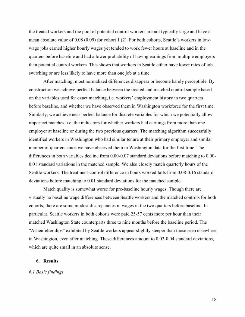
Figure 1 plots the increase in control group mean wages referenced above along with quantiles
for the same group. Three quarters after baseline, the 25th percentile and median wages for those
individuals still employed in Washington State lie below $11; only a minority of workers
initially employed at wages below that figure will cross the threshold in the course of a year.12
The mean wage in follow-up quarters is close to the 75th percentile of the distribution, indicating
10 Some portion of this increase may reflect selective attrition by lower-earning workers. 11 Note that both the duration of current spell and time since entry variables are truncated at 41 quarters, implying that these measures understate the true means. 12 This could be taken as evidence that wage mobility has declined in the period since Smith and Vavrichek (1992) and Long (1999). Note, however, the difference in methods: these prior studies examined workers earning exactly the minimum wage, here we focus on those earning up to $1.53 above the minimum.
10
a pronounced skew. This skew might reflect a subset of the low-wage workforce enrolled in
educational or training programs at baseline leading to significantly higher wages upon
completion.
4.2 Workers in low-wage jobs exhibit “Ashenfelter dips”
While the summary statistics presented above suggest that the low-wage labor market
incorporates workers on both upwardly mobile and stagnant trajectories, data also point to the
prevalence of negative shocks among workers earning low wages at a discrete point in time.
Among workers employed at the lowest wages in a given quarter, average wages conditional on
employment exhibit a downward trend leading into that quarter (see Table 3). In our Washington
State control sample, workers earned an average of $10.06 per hour in the 1st quarter of 2015, a
decline from the $10.98 observed just six months prior.
Workers might experience these hourly wage declines for any number of reasons. They
may experience layoffs from one job and quickly accept a new one offering a lower rate.
Overtime or bonus pay, which raises observed hourly wages in our data, might fluctuate
seasonally. Regardless of the cause, if the negative shocks impacting workers in low-wage jobs
are transitory “Ashenfelter dip” phenomena (Ashenfelter, 1978), it would be reasonable to expect
mean reversion in the calendar quarters immediately after baseline. Both mean reversion and
wage gains associated with greater experience and productivity suggest we should expect upward
trajectories among those employed for the lowest wages at any single point in time.
4.3 Few low-wage jobs offer full-time hours; separation rates are high
Low-wage work is predominantly part-time work, at least in our data. Members of our
control group averaged 237 hours worked in the first quarter of 2015 – around 18 hours per week
if averaged over 13 weeks (see Table 3). This figure may be an underestimate if some workers in
the data did not work the full 13 weeks, for example if they were hired into or separated from
their employer mid-quarter. Approximately 93% of the control sample logged less than full-time
full-quarter work (i.e. 520 hours) in the baseline period.
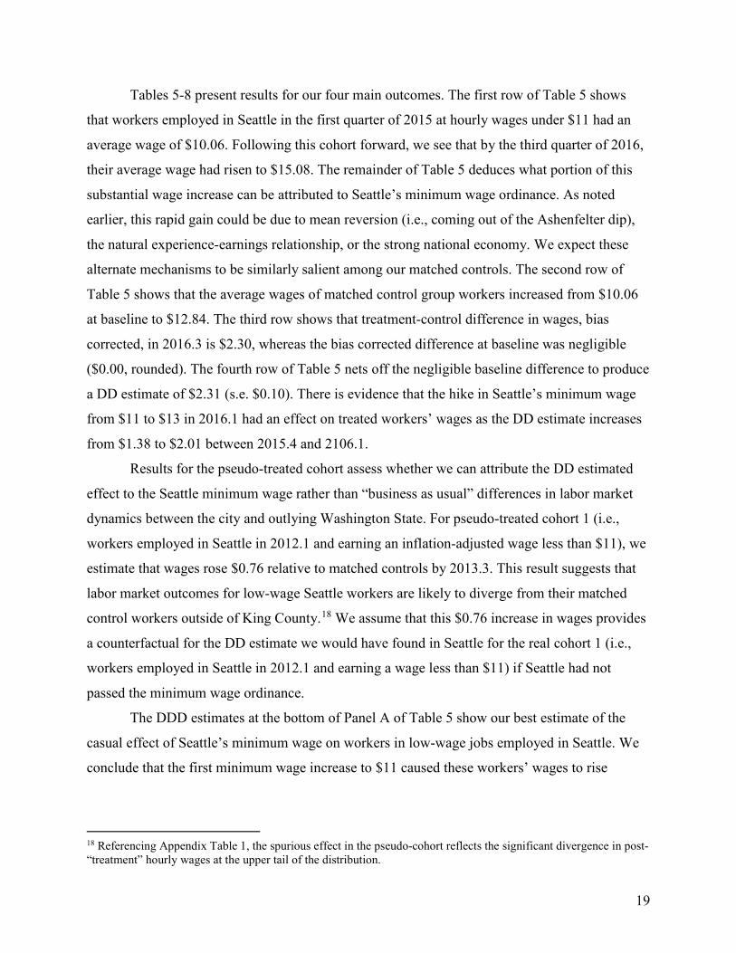
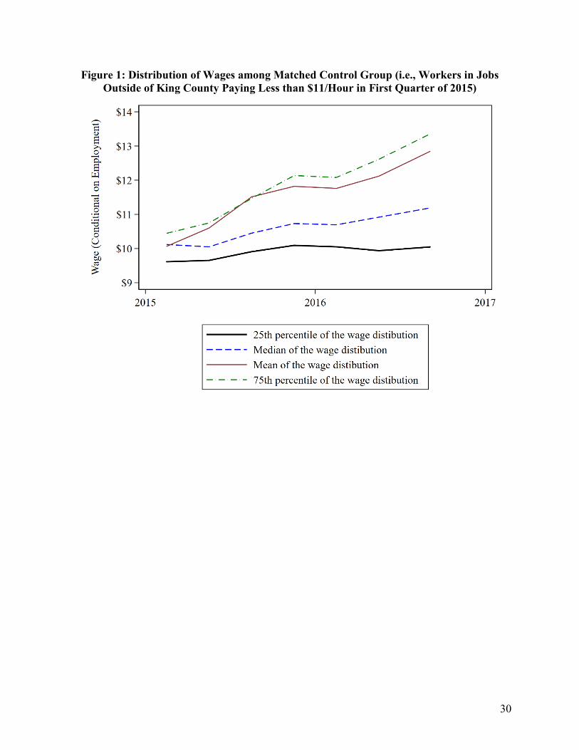
Among low-wage employment spells beginning at any point in time, only about one in
three will survive a full year. Figure 2 shows two, four, six, and eight-quarter survival rates for
low-wage employment spells in locatable Seattle businesses as a function of origination quarter,
11
beginning in 2005. Survival rates exhibit clear periodicity, with summer jobs being particularly
unlikely to persist. Around two-thirds of low-wage jobs beginning in any quarter will persist into
the next; about a third will last four quarters; less than a quarter will persist for six quarters, and
roughly one in six will last a full eight quarters. There is some evidence of increased job
persistence over the time period shown here, possibly reflecting the declining impact of the
2007-2009 recession on spell duration.
While most low-wage jobs commencing at any one point in time are destined for
separation within a year, recall that among workers observed in a baseline quarter the mean
duration is more than five quarters. The low-wage labor market includes both a segment cycling
quickly through employment and a more persistent segment.
Among workers who exit from a low wage employment spell, a considerable number do
not re-appear with another job in Washington within the following calendar quarter. In our
control group, more than one in four workers in low-wage jobs observed in the first calendar
quarter of 2015 could not be found in administrative records for the fourth quarter. This does not
necessarily indicate that these individuals had no job for the full three months of the fourth
quarter. They may have transitioned to work out-of-state, to work as a contractor rather than
wage earner, to self-employment, or to other forms of work not reported to ESD.
Conditional on persisting in the same job, many workers in low-wage jobs receive a raise.
Figure 3 shows the probability that a worker initiating a spell at a wage under $15 transitions to a
wage above $15 after 2, 4, 6, or 8 quarters, conditional on the spell surviving. After two quarters,
about 30% of continuing workers have transitioned above the $15 threshold. This proportion
progressively increases to the eight-quarter mark, where over 60% of surviving employment
spells have transitioned to a wage of at least $15 except for those spells commencing during the
2007-2009 recession.13 This reinforces the takeaway point in section 4.1: maturation out of low-
wage labor markets occurs regularly but not universally.
4.4 Implications for empirical analysis
13 It is interesting to note the drop-offs in wage transition probabilities at the very end of the graph. These coincide with spells tracked into calendar year 2017, a period during which the minimum wage in both Seattle and Washington State increased. These results suggest that the third minimum wage increase in 2017 was funded in part by holding back on wage upgrading above $15 for workers with a modest degree of experience.
12
Together, the phenomena documented here imply a challenge for evaluating the impact
of a minimum wage increase on a longitudinally-tracked cohort. Starting in any baseline period,
some workers may witness natural wage gains that render the increased minimum irrelevant
upon phase-in. Others will disappear from the data entirely, and it isn’t clear whether these
departures should be coded as transitions to non-employment or to employment not tracked by
one state’s UI system. And using an early baseline quarter causes the analysis to overlook a key
segment of the low-wage labor market: those who have only recently entered it. For these
reasons analysis of a cohort tracked from too early a point in time may reveal very small impacts
on wages, employment, and earnings.
These phenomena also indicate challenges in tracing impacts well beyond a minimum
wage phase-in. Over time, the segment of any longitudinal cohort which we expect to continue to
exhibit policy impacts will dwindle, as some workers disappear from the data and others
experience wage increases beyond the level where it is reasonable to expect impact.
The obvious strategy for circumventing these problems involves tracking a cohort from a
baseline period immediately preceding any minimum wage increase for only a modest length of
time afterward. This strategy may yield misleading evidence, however, to the extent that the
labor market anticipates minimum wage increases. To the extent anticipation effects exist, the
observed sample of low-wage earners would be selected, a group that was not offered
anticipatory wage increases perhaps because they are less highly valued by their employer.
Studying this group would then omit an important part of the story linking minimum wage
increases to individual trajectories.
Fortunately, prior evidence on the impact of Seattle’s minimum wage ordinance indicates
there were few if any anticipatory effects (Jardim et al., 2018a). Theoretically, in a less-than-
fully competitive labor market firms may bid up wages for more productive workers in advance
of a minimum wage increase. The absence of anticipation effects could reflect the relatively high
degree of competition in a growing urban labor market, or seasonal counter-effects associated
with implementing wage increases during or near the labor market’s natural trough.
With a short-duration panel, we are unable to study any longer-term implications of the
minimum wage. These long-run implications could be very important: to the extent higher
minimum wages reduce employment prospects for workers with no prior experience, policy
13
makers should want to understand whether these workers find some route into the labor market,
either by pursuing training outside the formal labor market or random luck.
5. Methodology
We use a difference-in-differences-in-differences (DDD) framework to estimate the
effect of Seattle’s first two phased minimum wage increases. In brief, this method contrasts the
differences in treated and control workers’ outcomes in quarters after enforcement of the
Ordinance to differences observed at baseline (difference-in-differences) and then difference this
result from the same exercise applied to a placebo cohort of Seattle and outlying Washington
workers observed in an earlier period of time when there was no local minimum wage law.
5.1 Identifying the “treated” sample of interest
Seattle’s minimum wage is imposed on employers rather than workers, which creates a
challenge for assigning treatment status to individual workers. The Ordinance covers work done
within the city boundaries of Seattle, defined by the physical location of the employer or the
workplace if the work is done outside of the employer’s premises. Movements of workers to and
from Seattle’s labor market can be thought of as non-compliance in terms of traditional treatment
effect literature. Given this worker mobility, our estimated effects can be considered “intent to
treat” (ITT).
We define workers assigned to treatment as those with 100 percent of their baseline
quarter (2015.1) employment in locatable Seattle businesses and who earned at least $8 but less
than $11 per hour in that quarter. We track these “Cohort 1” workers for the six following
quarters (2015.2 – 2016.3). We compare these treated workers to workers in Washington State
who received all of their earnings from locatable employers outside of King County in the
relevant baseline quarter but were otherwise similar to Seattle workers in terms of their recent
employment history and earnings.
We also report findings for “Cohort 2” treated workers, defined as those who had 100
percent of their baseline quarter (2015.4) employment in locatable firms in Seattle and earned at
least $8 but less than $13 per hour in that quarter. We track those workers for the three
subsequent quarters (2016.1 – 2016.3). Note that this cohort may have been endogenously
selected as their employment in Seattle could have been affected by the first minimum wage
14
increase to $11. If the first minimum wage increase had a disemployment effect, then Cohort 2
would consist of the workers who “survived” this first minimum wage hike. We present results
with this caveat in mind.
5.2 Matching methods and pseudo-cohort differencing
Rather than utilize the entire sample of wage-eligible workers outside King County as
controls, we apply a nearest neighbor matching strategy to minimize observed treatment-control
differences in baseline characteristics. Matching methods are often criticized on the grounds that
narrowing observable differences between treated and control observations can actually
exacerbate unobserved differences. These concerns are amplified in scenarios where individuals
faced a personal choice regarding whether to obtain the treatment. In this case, selecting
“control” observations with no employment in King County in a baseline period before the
treatment was actually implemented mitigates the concern. As we discuss below, concerns
regarding non-match on unobservables persist and we address them by differencing results
between a treated and untreated cohort.
For each treated worker, we identify the nearest neighbor without replacement.14 We
match exactly on workers’ employment status and whether they were first observed in
Washington State data in the three quarters prior to each minimum wage hike – the baseline
quarter as well as the two prior quarters. In addition, we continuously match workers on
quarterly hours worked in all jobs in the baseline quarter and each of the two prior quarters,
hourly wages (conditional on employment) in each of three quarters, having earnings from more
than one employer in a quarter (conditional on employment), the number of quarters a worker
has been linked to their current primary employer, and the number of quarters since the worker
first appeared in Washington State data. These duration measures are left-censored for workers
whose employment history extends before 2005. We use Mahalanobis (1936) distance, 𝐷𝐷𝑖𝑖𝑖𝑖 , to
measure the distance between individual 𝑖𝑖 and individual 𝑗𝑗, defined as:
14 Nearest neighbor without replacement is recommended by Abadie and Spiess (2016) so as to derive valid standard errors. For inference, we follow their suggestion of using a non-parametric block bootstrap that resamples matched-pairs of treatment and control workers. We produce 1,000 block bootstrapped samples for each point estimate. Alternate models using nearest neighbor matching with replacement and one to four matches yield point estimates similar to those presented here. There are tradeoffs in the choice of the number of matches. While increasing the number of neighbors allows for a more stable control group and reduces the variance of the estimates, it comes at the expense of allowing lower quality matches into the sample.
15
𝐷𝐷𝑖𝑖𝑖𝑖 = �𝑋𝑋𝑖𝑖 − 𝑋𝑋𝑖𝑖�′Σ−1�𝑋𝑋𝑖𝑖 − 𝑋𝑋𝑖𝑖�,
where Σ is the sample-covariance matrix of the covariates, 𝑋𝑋, in the pool of potential control
workers.
The first difference in the DDD estimator is the difference between the mean outcomes of
treatment and control workers in quarter 𝑞𝑞 following an increase in Seattle’s minimum wage
(with 𝑞𝑞 ranging from 1 to 6 for cohort 1 and 1 to 3 for cohort 2). This difference can be
represented as follows:
1𝑁𝑁𝑇𝑇𝑇𝑇𝑇𝑇𝑇𝑇𝑇𝑇𝑇𝑇𝑇𝑇
� �𝑌𝑌𝑖𝑖𝑖𝑖� −𝑁𝑁𝑇𝑇𝑇𝑇𝑇𝑇𝑇𝑇𝑇𝑇𝑇𝑇𝑇𝑇
𝑖𝑖=1
1𝑁𝑁𝑇𝑇𝑇𝑇𝑇𝑇𝑇𝑇𝑇𝑇𝑇𝑇𝑇𝑇
� �𝑌𝑌𝑖𝑖𝑖𝑖�2𝑁𝑁𝑇𝑇𝑇𝑇𝑇𝑇𝑇𝑇𝑇𝑇𝑇𝑇𝑇𝑇
𝑖𝑖=𝑁𝑁𝑇𝑇𝑇𝑇𝑇𝑇𝑇𝑇𝑇𝑇𝑇𝑇𝑇𝑇+1
with the observations sorted by treatment status such that treated observations are indexed from
𝑖𝑖 = 1 to 𝑖𝑖 = 𝑁𝑁𝑇𝑇𝑇𝑇𝑇𝑇𝑇𝑇𝑇𝑇𝑇𝑇𝑇𝑇 and their matched control observations are indexed from 𝑖𝑖 = 𝑁𝑁𝑇𝑇𝑇𝑇𝑇𝑇𝑇𝑇𝑇𝑇𝑇𝑇𝑇𝑇 + 1
to 𝑖𝑖 = 2𝑁𝑁𝑇𝑇𝑇𝑇𝑇𝑇𝑇𝑇𝑇𝑇𝑇𝑇𝑇𝑇.
Because we match on several continuous covariates, the matching estimator which
compares each observation to its neighbors may be biased (Abadie and Imbens 2011). We follow
Abadie and Imbens (2011) and implement bias-correction by running a regression of the
outcome of interest on the continuous covariates using the sample of the treated observations to
obtain �̂�𝛽1 and repeating with the sample of control observations to obtain �̂�𝛽0. We then compute
the bias-corrected difference between the mean outcomes of treatment and control workers in
The second difference in the DDD estimator takes the difference between the bias-
corrected difference for quarter 𝑞𝑞 (post-minimum wage hike) and the bias corrected difference
for the baseline quarter, 𝑞𝑞 = 0 (i.e., the quarter before the minimum wage hike). As shown in the
following section, these baseline differences are typically very small.
The third difference takes the difference between the DD estimate and a DD estimate
produced for a pseudo-treated cohort. This third difference controls for the possibility that Seattle
workers may diverge from their matched counterparts in the rest of the state for reasons
unrelated to the minimum wage ordinance. While our procedure ensures that treated and control
workers match closely on pre-treatment characteristics, control workers may face very different
16
local labor market conditions.15 To assess this possibility, we estimate the effect of a pseudo
minimum wage ordinance on pre-policy data. We impose a pseudo minimum wage ordinance
beginning in the second quarter of 2012 and identify treated workers as workers who earn less
than $11 per hour in 2015.2 dollars and who have 100 percent of their earnings in locatable firms
in Seattle or outside King County in the quarter prior (2012.1) – this is our pseudo-Cohort 1.16
We then follow them for six quarters after the pseudo minimum ordinance, 2012.2-2013.3. We
define pseudo-Cohort 2 as workers who earn less than $13 per hour and who have 100 percent of
their earnings in locatable firms in Seattle or outside King County in 2012.4, the baseline quarter
for the second pseudo minimum wage increase, and follow workers in the three quarters after,
2013.1 – 2013.3. We utilize the same matching process described above and estimate the DD for
each of the pseudo cohorts.
Our methodology is thus robust to differences in labor market conditions between treated
workers and matched controls, so long as the nature of those differences remained stable
between cohorts but for Seattle’s minimum wage increase.
In addition to deriving overall treatment effects, we test whether the effects of the
minimum wage vary by worker experience. We split workers into two groups based on the sum
of hours worked in the baseline and prior two quarters. For cohort 1 (2), we use a threshold of
582 (700) hours, which is the median number of hours worked by Seattle workers in the baseline
15 Appendix Figure 1 provides evidence of important divergence in labor market dynamics at the top-end of the wage distribution between “pseudo-treated” workers and matched controls drawn from Washington State outside of King County. The figure shows quantiles from the hourly wage distribution in the 4th quarter of 2012 for workers who were earning less than $11 per hour in the 1st quarter of 2012. At most quantiles, up to the 75th percentile, hourly wages for Seattle workers are quite similar to their matched controls, consistent with the assumption of parallel trends post-pseudo-treatment. The 95th and 99th percentiles, however, show Seattle workers well ahead of their counterparts. At these percentiles matched control workers have hourly wages of roughly $17 and $27, respectively, while Seattle workers at the same percentiles see wages of roughly $19 and $31. It appears that the upper tail of the distribution reflects individuals who accelerate rapidly out of the low-wage labor market, for example because they complete an educational degree or training program and transition to higher-skilled work. These opportunities may be more plentiful in the City of Seattle, which is home to approximately one-tenth of Washington’s population but more than one-sixth of the state’s colleges according to the U.S. Department of Education. Among the city’s 13 postsecondary institutions is the state’s largest by enrollment, the University of Washington. This phenomenon also appears in figures analogous to Appendix Figure 1, suggesting that this is a relatively permanent characteristic of the Seattle labor market. 16 Note that we chose 2012.1 as a starting point because (a) it is sufficiently early that when followed for six quarters hence (i.e., to 2013.3) it is still pre-passage of the Seattle minimum wage ordinance, (b) by beginning in a first quarter, we are comparing workers employed at the same calendar quarter as the real cohort 1 which is followed from 2015.1, and (c) it is sufficiently after the Great Recession of 2007.4 to 2009.2 (NBER, 2018) such that we can reasonably assume that labor market outcomes for this pseudo-treated cohort are a counterfactual for the actually treated cohort.
17
and prior two quarters. We apply these same thresholds to control workers and workers in the
pseudo cohorts.17 Figures 4 and 5 plot the distribution of hours worked by treatment and control
workers in cohorts 1 and 2, respectively, and illustrate that there are a large number of workers in
low-wage jobs with very low hours and a more modest group – roughly one in ten – working
full-time (1,560 hours) or more for the full period. For each subsample, we compute the DDD
estimates described above. Finally, we difference the results for less experienced workers with
more experienced workers to produce a DDDD estimate. We again use a block bootstrapping
procedure to produce standard errors for the DDDD estimates.
We focus on four general outcomes of interest. First, we study if Seattle’s minimum wage
has affected workers’ hourly wages for those workers who remain employed (i.e., the first order
effect desired and expected by policymakers). Second, we evaluate workers’ probability of being
employed anywhere in the state, including jobs with non-locatable employers and/or jobs outside
of Seattle. Third, we look at the impacts of the minimum wage on hours worked, setting hours
worked to zero for workers not observed in the data in a given quarter. Finally, we study if the
minimum wage led to gains in earnings for workers in low-wage jobs (the principal aim of
policymakers), again assigning a value of zero to workers not observed in employment data in a
given quarter.
To parse the findings on employment and hours, we examine two supplementary
outcomes. We assess the probability that workers remain employed by their baseline employer,
or equivalently job turnover. We also differentiate impacts on hours worked inside and outside
the city.
5.3 Assessing match quality
For Cohorts 1 and 2 respectively, Tables 3 and 4 compare pre-policy covariates for
treated workers, the pool of potential control workers (i.e., all workers in low-wage jobs in
Washington employed outside of King County at baseline), and the control workers chosen as
nearest neighbors. As a measure of balance, we present the normalized differences in covariates
between treated and control workers. Even prior to matching, normalized differences between
17 Our current analysis uses the same hours threshold for cohort 1 and pseudo-cohort 1, 582 hours, even though the median differs slightly across cohorts. To test the sensitivity of this choice, we also estimated effects using the median hours threshold for pseudo-cohort 1 rather than 582 hours; this threshold change did not affect the results.
18
the treated workers and the pool of potential control workers are not typically large and have a
mean absolute value of 0.08 (0.09) for cohort 1 (2). For both cohorts, Seattle’s workers in low-
wage jobs earned higher hourly wages yet tended to work fewer hours at baseline and in the
quarters before baseline and had a lower probability of having earnings from multiple employers
than potential control workers. This shows that workers in Seattle either have lower rates of job
switching or are less likely to have more than one job at a time.
After matching, most normalized differences disappear or become barely perceptible. By
construction we achieve perfect balance between the treated and matched control sample based
on the variables used for exact matching, i.e. workers’ employment history in two quarters
before baseline, and whether we have observed them in Washington workforce for the first time.
Similarly, we achieve near perfect balance for discrete variables for which we potentially allow
imperfect matches, i.e. the indicators for whether workers had earnings from more than one
employer at baseline or during the two previous quarters. The matching algorithm successfully
identified workers in Washington who had similar tenure at their primary employer and similar
number of quarters since we have observed them in Washington data for the first time. The
differences in both variables decline from 0.00-0.07 standard deviations before matching to 0.00-
0.01 standard variations in the matched sample. We also closely match quarterly hours of the
Seattle workers. The treatment-control difference in hours worked falls from 0.08-0.16 standard
deviations before matching to 0.01 standard deviations for the matched sample.
Match quality is somewhat worse for pre-baseline hourly wages. Though there are
virtually no baseline wage differences between Seattle workers and the matched controls for both
cohorts, there are some modest discrepancies in wages in the two quarters before baseline. In
particular, Seattle workers in both cohorts were paid 25-57 cents more per hour than their
matched Washington State counterparts three to nine months before the baseline period. The
“Ashenfelter dips” exhibited by Seattle workers appear slightly steeper than those seen elsewhere
in Washington, even after matching. These differences amount to 0.02-0.04 standard deviations,
which are quite small in an absolute sense.
6. Results
6.1 Basic findings
19
Tables 5-8 present results for our four main outcomes. The first row of Table 5 shows
that workers employed in Seattle in the first quarter of 2015 at hourly wages under $11 had an
average wage of $10.06. Following this cohort forward, we see that by the third quarter of 2016,
their average wage had risen to $15.08. The remainder of Table 5 deduces what portion of this
substantial wage increase can be attributed to Seattle’s minimum wage ordinance. As noted
earlier, this rapid gain could be due to mean reversion (i.e., coming out of the Ashenfelter dip),
the natural experience-earnings relationship, or the strong national economy. We expect these
alternate mechanisms to be similarly salient among our matched controls. The second row of
Table 5 shows that the average wages of matched control group workers increased from $10.06
at baseline to $12.84. The third row shows that treatment-control difference in wages, bias
corrected, in 2016.3 is $2.30, whereas the bias corrected difference at baseline was negligible
($0.00, rounded). The fourth row of Table 5 nets off the negligible baseline difference to produce
a DD estimate of $2.31 (s.e. $0.10). There is evidence that the hike in Seattle’s minimum wage
from $11 to $13 in 2016.1 had an effect on treated workers’ wages as the DD estimate increases
from $1.38 to $2.01 between 2015.4 and 2106.1.
Results for the pseudo-treated cohort assess whether we can attribute the DD estimated
effect to the Seattle minimum wage rather than “business as usual” differences in labor market
dynamics between the city and outlying Washington State. For pseudo-treated cohort 1 (i.e.,
workers employed in Seattle in 2012.1 and earning an inflation-adjusted wage less than $11), we
estimate that wages rose $0.76 relative to matched controls by 2013.3. This result suggests that
labor market outcomes for low-wage Seattle workers are likely to diverge from their matched
control workers outside of King County.18 We assume that this $0.76 increase in wages provides
a counterfactual for the DD estimate we would have found in Seattle for the real cohort 1 (i.e.,
workers employed in Seattle in 2012.1 and earning a wage less than $11) if Seattle had not
passed the minimum wage ordinance.
The DDD estimates at the bottom of Panel A of Table 5 show our best estimate of the
casual effect of Seattle’s minimum wage on workers in low-wage jobs employed in Seattle. We
conclude that the first minimum wage increase to $11 caused these workers’ wages to rise
18 Referencing Appendix Table 1, the spurious effect in the pseudo-cohort reflects the significant divergence in post-“treatment” hourly wages at the upper tail of the distribution.
20
between $0.63 and $0.88, and the second increase to as much as $13 caused an increase between
$1.22 and $1.54.
Panel B of Table 5 shows estimates for Cohort 2. Our results suggest that the minimum
wage hike to as much as $13 boosted their wages between $0.78 and $0.88. This increase is a bit
larger than the jump in wages for cohort 1. For example, for cohort 1, the jump in the DDD
estimate between 2015.4 and 2016.1 is $0.47 (i.e., $1.35-$0.88), which is smaller than the $0.83
DDD estimate in 2016.1 for cohort 2. The difference could reflect treatment effect heterogeneity,
given the difference in selection criteria between the two cohorts, but might also reflect
endogenous selection into cohort 2.
Table 6 shows, broadly speaking, no evidence that the Seattle minimum wage reduced
the probability of employment among those employed in the quarters prior to the law’s
implementation. The DD estimates show that cohort 1 (cohort 2) treated workers were 1.1 (2.3)
percentage points more likely to be employed in 2016.3 than their matched control workers. The
pseudo cohorts suggest that some of this apparent gain is an expected phenomenon for Seattle
workers as pseudo-cohort 1 (pseudo-cohort 2) was 0.6 (1.3) percentage points more likely to be
employed in 2013.3 than their matched comparisons. The DDD estimates are statistically
insignificant for cohort 1 (ranging from -0.8 to +0.5 percentage points), while the DDD estimates
are each significant at the 10% level for cohort 2, but of various signs (-0.8, -0.8, and +1.0
percentage points).
Table 7 indicates that Seattle workers worked significantly fewer hours per quarter as a
result of the minimum wage hikes. The DDD results show significant declines in hours worked
in all six quarters for cohort 1 ranging from -6.3 to -14.1 hours per quarter, or 30 to 60 minutes
per week. The DDD results for cohort 2 range from -3.0 to -11.5 and are significant for two of
the three quarters following the increase in the minimum wage to $13. The DDD estimates for
hours worked are fairly similar to the DD estimates for cohort 1 and 2 as the estimated DD
effects for the pseudo cohorts are usually small and insignificant. Together, tables 5 and 7
suggest that incumbent treated workers experienced potentially offsetting effects -- an increase in
hourly wages coupled with a decline in hours worked. They also indicate the importance of
analyzing employment effects on both the extensive and intensive margins.
Table 8 assesses whether these opposing forces resulted in higher or lower quarterly
earnings for treated workers. Baseline earnings for Seattle’s cohort 1 workers averaged $2,417 in
21
2015.1. Mean quarterly earnings rose to $3,531 by 2015.6, and this growth exceeded the gains
for the matched control workers, yielding a DD estimate of $416. Almost half of this gain can be
attributed to business as usual as pseudo-treated workers experienced a relative gain of $195.
The net DDD estimate suggests that the Seattle minimum wage caused a $221 quarterly earnings
gain for cohort 1 workers in 2016.3.
For cohort 1, we find gains ranging from $90 to $221 during the three quarters of 2016,
an average of $12 per week, while for cohort 2, we find gains ranging from $25 to $190 during
the three quarters of 2016, an average of $8 per week. Thus, while prior estimates conclude the
total amount paid to low wage workers in Seattle declined by 6-7 percent (Jardim et al., 2018),
the workers in cohort 1 (2) who were employed at baseline saw average earnings gains of 6.3
(3.2) percent. These results suggest the effects of the Seattle minimum wage were heterogeneous
and depended to some extent on workers’ labor market experience prior to the hikes. We
examine this suggestion by stratifying our sample of employed workers on the basis of their prior
experience.
6.2 Heterogeneity in Effects Based on Prior Experience
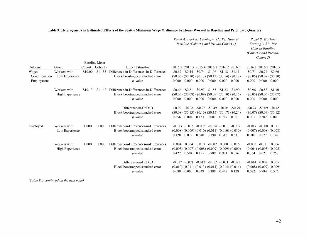
Table 9 presents evidence in support of the hypothesis that the Seattle minimum wage
was more beneficial to experienced workers. First, we find that workers with above median
number of hours worked in the baseline quarter and prior two quarters saw their wages rise a bit
more than less experienced workers, conditional on employment. For the three quarters of 2016,
the estimated DDD estimates range from $0.83 to $1.90 for more experienced workers versus
$0.71 to $1.11 for less experienced workers. The DDDD estimates show that this disparity is
statistically significant for five of the nine quarters evaluated, and all of these five estimates
favor more experienced workers.
The relatively modest impacts on the probability of employment observed in Table 6
above persist when we split the sample by experience. However, there is suggestive evidence of
greater disemployment among the less experienced. Averaging across the estimates for 2016, we
find a DDD effect of -0.7 percentage points for the less experienced, and +0.1 percentage points
for the more experienced. Three of the nine DDDD estimates are negative and significant at the
10% level.
22
Both experience groups witnessed significant declines in hours worked. The DDD
estimates for 2016 range from -1.1 to -12.5 and average -7.8 for the less experienced. They
ranged and from -5.6 to -15.8 and average -11.4 for the more experienced. While the point
estimates tend to be a bit larger for the more experienced, it is important to note that the base
number of hours worked for these two groups differed substantially. Less experienced workers
worked 108.6 (142.2) hours during the baseline quarter for cohort 1 (2), while more experienced
workers worked 367.1 (432.2) hours during the baseline quarter for cohort 1 (2). Consequently,
the DDD estimates represent a substantial percentage decline in hours worked for less
experienced workers, while reflecting a much more modest percentage effect for more
experienced workers.
The bottom of Table 9 presents the most striking findings. For less experienced workers,
the gain in hourly wages was offset by the decline in hours yielding small and insignificant net
impacts on earnings. In contrast, all of the nine estimated DDD estimates for effects on earnings
are positive and significant for more experienced workers. For the three quarters of 2016, the
DDD estimates average to $12 per quarter for the less experienced and $251 per quarter (or $19
per week) for the more experienced.
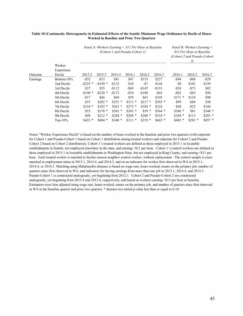
Table 10 provides further detail, dividing workers into deciles on the basis of hours
worked in the three quarters prior to each minimum wage increase. Table 9’s general conclusion
– that roughly half of all workers enjoyed significant earnings increases, while the less
experienced half effectively broke even – continues to hold. Individuals in the highest decile of
cohort 1, who worked at least 1,471 hours in the nine month base period, or an average of 38
hours per week, show particularly noteworthy impacts. These workers saw a combination of
significantly higher earnings and reduced hours. It is conceivable that the observed hours
reductions reflect voluntary cutbacks in work effort, given the high level of exertion observed at
baseline and the fact that these workers retain enough hours to boost their weekly earnings by as
The results of this longitudinal analysis contrast strikingly with repeat cross-section
analyses suggesting sharper reductions in hours worked in Seattle’s low wage labor market in
2016 (Jardim et al., 2018a). These findings could be compatible for multiple reasons. First,
23
longitudinal analysis by necessity excludes workers who enter Seattle’s low-wage workforce
after the baseline period, or who never enter at all. Second, individual workers may be making
up for lost work in Seattle by adding employment outside the city limits. Our decision to include
all Washington state employment and earnings might mask steeper employment and hours
declines in the city. The top panel of Table 11 explores this second mechanism of adjustment.
In the full sample we do not find an increase in hours worked outside the city. We do,
however, find significant increases in outside-of-Seattle hours among more experienced workers,
with 5 of 9 estimated coefficients statistically significant at the 5% level and a sixth with a p-
value of 0.106. Averaged across quarters, the effect amounts to about 7 hours per quarter or just
over 30 minutes per week. Taken in the context of our results on overall hours worked, these
results indicate that experienced workers had some capacity to offset hours reductions in Seattle
by finding work outside the city. While the effect is modest in magnitude, it implies that a non-
negligible portion of the weekly earnings increases accruing to more-experienced workers can be
attributed to increased work outside the city.19
By contrast, point estimates suggest less experienced workers in low-wage jobs decreased
their hours worked outside the city by around 3 hours per quarter. The differences in estimated
effects between more- and less-experienced workers are statistically significant at the 5% level in
6 of the 9 cases evaluated, and at the 10% level in one case.
The bottom panel of Table 11 explores whether workers were more likely to remain
employed by their baseline employer, conditional on being employed. Given the higher
minimum wage, employers have an incentive to retain their employees assuming that labor
productivity is an increasing function of tenure. Higher wages may also increase incentives for
workers to continue working for their current employer.
We find evidence consistent with this hypothesis. Workers are 1 to 4 percentage points
more likely to be employed at their baseline employer conditional on being employed, and these
estimated effects are significant at the 10% level in 8 of the 9 cases evaluated. Estimated
turnover effects tend to increase in magnitude over time. After six quarters, roughly half of our
matched controls and placebo cohorts continued to be employed by their baseline employer,
indicating a turnover rate of 50%. The near-4 percentage point reduction in turnover found in
19 Valuing hours outside the city at the state minimum wage of $9.47, the results suggest that about one-quarter of the earnings gains for experienced workers reflect increased work outside the city.
24
the sixth quarter of treatment thus amounts to an 8% drop in turnover. We find no significant
heterogeneity in this effect by worker experience. These results confirm recent empirical studies
on minimum wages’ impacts on job turnover that used proxies for the low-wage labor market
(Dube, Lester and Reich, 2016; Gittings and Schmutte, 2016).
6.4 Reductions in Opportunities for Potential Labor Market Entrants
This analysis focuses on individuals employed at baseline. To be included in the
treatment group, these workers must have had some work experience by the time Seattle’s
minimum wage increased, and that work experience may set them apart from inexperienced
workers attempting to enter the Seattle low-wage labor market. Job seekers who lack any labor
market experience in Washington are invisible to us, as they do not appear in administrative
records. We can infer their trajectories by studying aggregate statistics on the number of new
entrants into the Seattle low-wage labor market.
Figure 5 presents evidence on new entrants. In this figure, a “new entrant” is defined as a
worker who had not been employed in Washington State in the prior five years.20 We show 4-
quarter moving averages of the raw number of new entrants to eliminate strong seasonality in
labor market entry. We then normalize the two time series with different natural scales,
multiplying by 100 and dividing by the 4-quarter moving average in 2014.2 (i.e., we set 2014.2,
the quarter before passage of the ordinance, at 100). Around this baseline period, both Seattle
and outlying Washington State show signs of accelerating growth in the low-wage labor market,
with the number of new entrants growing at a comparable rate. These two trends diverge after
the baseline period. Seattle transitions from a period of growth to a period of stasis or modest
decline once the minimum wage increase take effect, despite its booming economy. Washington
State outside King County continues to see growth in the number of new entrants, stabilizing at a
higher level in mid-2015. Declines in jobs available to such new entrants to the low-wage labor
market, and other workers with little experience who were not employed at the baselines would
be reflected in Jardim et al.’s (2018a) analysis of the aggregate labor market, but would not be
captured by the longitudinal analysis in this paper.
20 Use of a “moving window” to identify new entrants is preferable to identifying new entrants as those with no prior appearance in the data, as this second selection criterion becomes systematically more stringent over time.
25
Combining the results of these two papers suggests an important lesson: Seattle’s
minimum wage ordinance appears to have delivered higher pay to experienced workers at the
cost of reduced opportunity for the inexperienced. This result is consistent with anecdotal,
survey, and interview evidence collected the UW Minimum Wage Study, in which employers
consistently emphasize an increased focus on experience in the hiring process.
7. Conclusion
A wide array of labor market interventions promise to expand work opportunities and
increase earnings for one group at the risk of reducing other groups’ employment opportunities.21
In the case of the minimum wage, academic debate persists regarding the existence and
magnitude of these trade-offs. But presuming that some trade-off exists, the normative question
of whether a higher minimum wage represents a fair and desirable labor market intervention
hinges on the positive question of which workers benefit and which do not. This positive
question has received scant attention from an otherwise voluminous literature on the impacts of
minimum wage policies.
Our analysis of over 14,000 workers employed at wages under $11/hour in early 2015, as
well as some 25,000 employed at wages under $13/hour at the conclusion of 2015, documents
the expected and intended impacts of Seattle’s minimum wage ordinance on hourly wages.
Evidence indicates that these workers experienced no significant decline in their likelihood of
being employed and a modest reduction in their hours worked over the six quarters following the
first and second wage increases. Taken together, the minimum wage law increased these
workers’ pretax earnings by average of around $10 per week. Further analysis indicates that
earnings gains were concentrated among more experienced workers, with the less-experienced
half of Seattle’s baseline low-wage workforce showing no significant change.
These findings contrast with our earlier work, which showed that the total amount paid
to workers in low-wage jobs in Seattle declined after the second minimum wage increase in 2016
(Jardim et al., 2018). While this could reflect Seattle workers transitioning to work outside the
city, evidence presented here points to a relative and absolute reduction in the flow of new
employees into the Seattle low-wage workforce as the key reconciling factor.
21 Examples include child labor laws, occupational licensing, and immigration restrictions.
26
Much remains to be learned. Our segmentation of the workforce into more- and less-
experienced portions is a crude first step at examining effect heterogeneity. Our research team is
in the process of creating a merged administrative data resource that would link sparse
employment records to drivers’ license records, voter registration records, and other agency
databases that promise to link individual workers into households and provide more demographic
information. This will enable analysis of workers according to gender, age, and family income
status.
As a final caveat, we emphasize that during the period under study Seattle was
undergoing an exceptional economic boom driven by rapid expansion of its high-skilled
workforce. This may have driven the wages of less-paid employees up relative to the remainder
of Washington State where our matched controls reside. Seattle workers exhibited a larger
“Ashenfelter dip,” on average, relative to controls and it is reasonable to think that some element
of the wage and earnings improvement documented here reflects a more significant rebound
rather than any minimum wage impact. Regardless of the underlying mechanisms, at a
documentary level the evidence here indicates that individuals employed in Seattle’s low-wage
workforce immediately before its first two minimum wage increases saw wage and earnings
growth that outpaced observationally similar workers in other parts of Washington State.
27
References Abadie, A. and Imbens, G.W., 2006. Large sample properties of matching estimators for average treatment effects. Econometrica, 74(1), pp. 235-267. https://doi.org/10.1111/j.1468-0262.2006.00655.x Abadie, A. and Imbens, G.W., 2011. Bias-corrected matching estimators for average treatment effects. Journal of Business & Economic Statistics, 29(1), pp.1-11. https://doi.org/10.1198/jbes.2009.07333 Abadie, A. and Spiess, J., 2016. Robust post-matching inference. Harvard University. Unpublished manuscript. https://scholar.harvard.edu/spiess/publications/robust-post-matching-inference Addison, J., Blackburn, M., and C. Cotti. 2008. New Estimates of the Effects of Minimum Wages in the U.S. Retail Trade Sector. IZA Discussion Paper No. 3597. Allegretto, S., Dube, A., Reich, M., and B. Zipperer. 2013. Credible Research Designs for Minimum Wage Studies. IRLE Working Paper No. 148-13 Ashenfelter, O. 1978. Estimating the Effect of Training Programs on Earnings. Review of Economics and Statistics, 60(1): 47-50. Card, D. and A. B. Krueger 1994. Minimum Wages and Employment: A Case Study of the Fast-Food Industry in New Jersey and Pennsylvania. The American Economic Review 84(4): 772-793. Carrington, W. J. and B. C. Fallick. 2001. Do Some Workers Have Minimum Wage Careers? Monthly Labor Review 124(5): 17-27. Cengiz, D., Dube, A., Lindner, A., and B. Zipperer. 2017. The Effect of Minimum Wages on the Total Number of Jobs: Evidence from the United States Using a Bunching Estimator. Working Paper presented at 2018 Allied Social Science Association meetings. https://www.aeaweb.org/conference/2018/preliminary/paper/DSbE66Rs Clemens, J. and M. Wither. 2016. The Minimum Wage and the Great Recession: Evidence of Effects on the Employment and Income Trajectories of Low-Skilled Workers. Working Paper. University of California at San Diego. http://econweb.ucsd.edu/~j1clemens/pdfs/ClemensWitherMinimumWageGreatRecession.pdf Currie, J., and B.C. Fallick. 1996. The Minimum Wage and the Employment of Youth: Evidence from the NLSY. The Journal of Human Resources 31(2): 404-428. Dube, A., S. Naidu, and M. Reich. 2007. The Economic Effects of a Citywide Minimum Wage Industrial & Labor Relations Review 60: 522-543
Dube, A., T. W. Lester and M. Reich. 2010. Minimum Wage Effects Across State Borders: Estimates using Contiguous Counties. The Review of Economics and Statistics 92(4): 945-964. Dube, A., T.W. Lester, and M. Reich. 2016. Minimum Wage Shocks, Employment Flows, and Labor Market Frictions. Journal of Labor Economics 34(3): 663-704. Even, W. E., and D.A. Macpherson. 2003. The Wage and Employment Dynamics of Minimum Wage Workers. Southern Economic Journal 69(3): 676-691. Gittings, R.J., and I.M. Schmutte. 2016. Getting Handcuffs on an Octopus: Minimum Wages, Employment, and Turnover. Industrial and Labor Relations Review 69(5): 1133-1170. Jardim, E., M. Long, R. Plotnick, E. van Inwegen, J. Vigdor and H. Wething. 2018a. “Minimum Wage Increases, Wages, and Low Wage Employment: Evidence from Seattle.” National Bureau of Economic Research Working Paper #23532 (second revision). Jardim, E., Long, M., Plotnick, R., van Inwegen, E., Vigdor, J., and H. Wething. 2018b. The Extent of Local Minimum Wage Spillovers. Working Paper. University of Washington. Lachowska, M., A. Mas, and S.A. Woodbury. 2018. “How Reliable Are Administrative Reports of Paid Work Hours?” Unpublished manuscript. Long, J. 1999. Updated Estimates of the Wage Mobility of Minimum Wage Workers. Journal of Labor Research 20(4): 493-503. Mahalanobis, P.C. 1936. On the Generalised Distance in Statistics. Proceedings of the National Institute of Sciences of India 2(1): 49–55. Meer, J. and J. West. 2016. Effects of the Minimum Wage on Employment Dynamics. Journal of Human Resources 51(2): 500-522. Murphy, Kevin M., and Finis Welch. "Empirical age-earnings profiles." Journal of Labor Economics 8.2 (1990): 202-229. Neumark, D. and W. Wascher, 1995. The Effect of New Jersey's Minimum Wage Increase on Fast-Food Employment: A Re-Evaluation Using Payroll Records. National Bureau of Economic Research, Working Papers 5224. Reich, M., S. Allegretto, and A. Godoey. 2017. Seattle’s Minimum Wage Experience 2015-16. Center on Wage and Employment Dynamics. http://irle.berkeley.edu/files/2017/Seattles-Minimum-Wage-Experiences-2015-16.pdf. Rinz, K. and J. Voorheis. 2018. The Distributional Effects of Minimum Wages: Evidence from Linked Survey and Administrative Data. Working Paper. U.S. Census Bureau. https://www.census.gov/content/dam/Census/library/working-papers/2018/adrm/carra-wp-2018-02.pdf
Smith, R. E. and B. Vavrichek. 1992. The Wage Mobility of Minimum Wage Workers. Industrial & Labor Relations Review 46(1): 82-88. Stewart, M. B. 2004. The Employment Effects of the National Minimum Wage. Economic Journal 114(494): C110-C116.
30
Figure 1: Distribution of Wages among Matched Control Group (i.e., Workers in Jobs Outside of King County Paying Less than $11/Hour in First Quarter of 2015)
31
Figure 2: Share of Employment Spells that Survive among Seattle Jobs Paying Less than $15/Hour at Beginning of Spell
Figure 3: Share of Employment Spells that Upgrade their Wage to > $15/Hour, Conditional on the Spell Having Survived, among Seattle Jobs Paying < $15/Hour at Beginning of Spell
32
Figure 4: Cohort 1’s Distribution of Prior Experience
Figure 5: Cohort 2’s Distribution of Prior Experience
33
Figure 5: Relative Decline in New Low-Wage Labor Market Entrants in Seattle
Note: A worker is defined as a new low-wage entrant if s/he becomes employed during the
quarter with a wage less than $15 and had not been observed as employed during the prior 20 quarters.
34
No benefits With benefitsb No benefits or tips Benefits or tipsc January 1, 2015 $9.47 $9.47 $9.47 $9.47
April 1, 2015 $11.00 $11.00 $11.00 $10.00January 1, 2016 $13.00 $12.50 $12.00 $10.50 January 1, 2016 $9.47January 1, 2017 $15.00d $13.50 $13.00 $11.00 January 1, 2017 $11.00January 1, 2018 $15.45 $15.00e $14.00 $11.50 January 1, 2018 $11.50January 1, 2019 $15.00f $12.00 January 1, 2019 $12.00January 1, 2020 $13.50 January 1, 2020 $13.50January 1, 2021 $15.00g
Notes:a bc
de
f
g
Table 1: Minimum Wage Schedule in Seattle and Washington State
Seattle Washington State
Effective DateLarge Employersa Small Employers All Employers
After the minimum hourly compensation for small employers reaches $15 it goes up to $15.75 until January 1, 2021 when it converges with the minimum wage schedule for large employers.The minimum wage for small employers with benefits or tips will converge with other employers by 2025.
A large employer employs 501 or more employees worldwide, including all franchises associated with a franchise or a Employers who pay towards medical benefits.
Employers who pay toward medical benefits and/or employees who are paid tips. Total minimum hourly compensations (including tips and benefits) is the same as for small employers who do not pay towards medical benefits and/or tips.For large employers, in the years after the minimum wage reaches $15.00 it is indexed to inflation using the CPI-W for
In subsequent years, starting January 1, 2019, payment by the employer of medical benefits for employees no longer affects the hourly minimum wage paid by a large employer.
Notes: Columns (3), (4), and (5) show the number excluded after sample exclusions shown in prior columns.
Table 2: Number and Share of Low-Wage Washington Workers Included in the Analysis
Number of WorkersLow-Wage Washington
Workers (Baseline Quarter)
Excluded from Analysis Because of Baseline Employment at: Included in Analysis
(Treated + Pool of
Potential Control
Workers)
Share Included
36
(3) (5)
Mean (S.D.) Mean (S.D.) Normalized Difference
from Treated
Mean (S.D.) Normalized Difference
from TreatedVariables Matched ExactlyEmployed in 2015.1 1.00 1.00 NA 1.00 NAEmployed in 2014.4 0.79 0.83 -0.10 0.79 0.00Employed in 2014.3 0.72 0.76 -0.10 0.72 0.00New Entrant in 2015.1 0.08 0.07 0.06 0.08 0.00New Entrant in 2014.4 0.05 0.05 0.03 0.05 0.00New Entrant in 2014.3 0.05 0.05 0.01 0.05 0.00
Variables Matched Non-ExactlyJob Tenure at Baseline (2015.1) Employer 5.6 (8.0) 5.6 (7.8) 0.00 5.5 (8.0) 0.01Potential Experience at Baseline (2015.1)) 20.4 (15.4) 21.4 (15.3) -0.07 20.4 (15.5) 0.00Hours Worked in 2015.1 240 (199) 261 (179) -0.12 237 (191) 0.01Hours Worked in 2014.4 227 (207) 255 (205) -0.14 225 (202) 0.01Hours Worked in 2014.3 216 (211) 251 (227) -0.16 214 (207) 0.01Wage in 2015.1 $10.06 ($0.51) $10.01 ($0.47) 0.11 $10.06 ($0.50) 0.00Wage in 2014.4 (Conditional on Employment) $11.09 ($6.24) $10.85 ($6.68) 0.04 $10.84 ($5.64) 0.03Wage in 2014.3 (Conditional on Employment) $11.46 ($12.48) $11.19 ($11.72) 0.02 $10.98 ($11.45) 0.03Earnings from More Than One Employer in 2015.1 0.048 0.084 -0.13 0.048 0.00Earnings from More Than One Employer in 2014.4 0.142 0.157 -0.04 0.112 0.00Earnings from More Than One Employer in 2014.3 0.162 0.204 -0.10 0.116 0.00
Mean of absolute values 0.08 0.01
Observations 14,409 164,184 14,409
(4)Pool of Potential Control Workers Matched Control Workers
Table 3: Balance Between Cohort 1's Treated Workers, Pool of Potential Control Workers, and Matched Control Workers
Notes: Data derived from administrative employment records obtained from the Washington Employment Security Department. Non-locatable employers and workers with employment in outlying King County are excluded. Cohort 1 is defined as workers employed in 2015.1 in locatable establishments in Washington State and earning <$11 per hour.
(1)Treated Workers
(2)
37
(3) (5)
Mean (S.D.) Mean (S.D.) Normalized Difference
from Treated
Mean (S.D.) Normalized Difference
from TreatedVariables Matched ExactlyEmployed in 2015.1 1.00 1.00 NA 1.00 NAEmployed in 2014.4 0.83 0.85 -0.07 0.83 0.00Employed in 2014.3 0.72 0.75 -0.05 0.72 0.00New Entrant in 2015.1 0.08 0.06 0.07 0.08 0.00New Entrant in 2014.4 0.06 0.06 0.00 0.06 0.00New Entrant in 2014.3 0.04 0.04 -0.02 0.04 0.00
Variables Matched Non-ExactlyJob Tenure at Baseline (2015.1) Employer 6.2 (8.8) 6.0 (8.6) 0.02 6.1 (8.8) 0.01Potential Experience at Baseline (2015.1)) 22.7 (16.6) 23.7 (16.6) -0.06 22.7 (16.7) 0.00Hours Worked in 2015.1 289 (214) 304 (198) -0.08 287 (208) 0.01Hours Worked in 2014.4 267 (222) 295 (225) -0.12 264 (216) 0.01Hours Worked in 2014.3 231 (221) 251 (225) -0.09 228 (217) 0.01Wage in 2015.1 $11.49 ($0.92) $10.94 ($1.08) 0.51 $11.48 ($0.91) 0.01Wage in 2014.4 (Conditional on Employment) $12.59 ($10.68) $11.86 ($9.67) 0.07 $12.16 ($10.24) 0.04Wage in 2014.3 (Conditional on Employment) $12.72 ($27.14) $11.39 ($8.59) 0.12 $12.15 ($17.88) 0.02Earnings from More Than One Employer in 2015.1 0.063 0.096 -0.12 0.062 0.00Earnings from More Than One Employer in 2014.4 0.159 0.191 -0.08 0.132 0.00Earnings from More Than One Employer in 2014.3 0.163 0.178 -0.04 0.118 0.00
Mean of absolute values 0.09 0.01
Observations 25,734 268,040 25,734
Notes: Data derived from administrative employment records obtained from the Washington Employment Security Department. Non-locatable employers and workers with employment in outlying King County are excluded. Cohort 1 is defined as workers employed in 2015.1 in locatable establishments in Washington State and earning <$11 per hour.
Table 4: Balance Between Cohort 2's Treated Workers, Pool of Potential Control Workers, and Matched Control Workers
(1) (2) (4)Treated Workers Pool of Potential Control Workers Matched Control Workers
Panel B: Workers Earning < $13 Per Hour at Baseline (Cohort 2
and Pseudo-Cohort 2)
Notes: Cohort 1’s treated workers are defined as those employed in 2015.1 in locatable establishments in Seattle, not employed elsewhere in the state, and earning <$11 per hour. Cohort 1’s control workers are defined as those employed in 2015.1 in locatable establishments in Washington State, but not employed in King County, and earning <$11 per hour. Each treated worker is matched to his/her nearest neighbor control worker, without replacement. The control sample is exact matched in employment status in 2015.1, 2014.4, and 2014.3, and on an indicator for worker first observed in WA in 2015.1, 2014.4, or 2014.3. Matching using Mahalanobis distance is based on wage rate, hours worked, tenure on the primary job, number of quarters since first observed in WA, and indicators for having earnings from more than one job in 2015.1, 2014.4, and 2014.3. Pseudo-Cohort 1 is constructed analogously, yet beginning from 2012.1. Cohort 2 and Pseudo-Cohort 2 are constructed analogously, yet beginning from 2015.4 and 2013.4, respectively, and based on workers earning <$13 per hour at baseline. Estimators were bias adjusted using wage rate, hours worked, tenure on the primary job, and number of quarters since first observed in WA in the baseline quarter and prior two quarters.
Table 5: Estimated Effect of the Seattle Minimum Wage Ordinance on Wages Conditional on Employment
Panel A: Workers Earning < $11 Per Hour at Baseline (Cohort 1 and Pseudo-Cohort 1)
Table 6: Estimated Effect of the Seattle Minimum Wage Ordinance on Employment
Panel A: Workers Earning < $11 Per Hour at Baseline (Cohort 1 and Pseudo-Cohort 1)
Panel B: Workers Earning < $13 Per Hour at Baseline (Cohort 2
and Pseudo-Cohort 2)
Notes: Cohort 1’s treated workers are defined as those employed in 2015.1 in locatable establishments in Seattle, not employed elsewhere in the state, and earning <$11 per hour. Cohort 1’s control workers are defined as those employed in 2015.1 in locatable establishments in Washington State, but not employed in King County, and earning <$11 per hour. Each treated worker is matched to his/her nearest neighbor control worker, without replacement. The control sample is exact matched in employment status in 2015.1, 2014.4, and 2014.3, and on an indicator for worker first observed in WA in 2015.1, 2014.4, or 2014.3. Matching using Mahalanobis distance is based on wage rate, hours worked, tenure on the primary job, number of quarters since first observed in WA, and indicators for having earnings from more than one job in 2015.1, 2014.4, and 2014.3. Pseudo-Cohort 1 is constructed analogously, yet beginning from 2012.1. Cohort 2 and Pseudo-Cohort 2 are constructed analogously, yet beginning from 2015.4 and 2013.4, respectively, and based on workers earning <$13 per hour at baseline. Estimators were bias adjusted using wage rate, hours worked, tenure on the primary job, and number of quarters since first observed in WA in the baseline quarter and prior two quarters.
Table 7: Estimated Effect of the Seattle Minimum Wage Ordinance on Hours Worked
Panel A: Workers Earning < $11 Per Hour at Baseline (Cohort 1 and Pseudo-Cohort 1)
Panel B: Workers Earning < $13 Per Hour at Baseline (Cohort 2
and Pseudo-Cohort 2)
Notes: Cohort 1’s treated workers are defined as those employed in 2015.1 in locatable establishments in Seattle, not employed elsewhere in the state, and earning <$11 per hour. Cohort 1’s control workers are defined as those employed in 2015.1 in locatable establishments in Washington State, but not employed in King County, and earning <$11 per hour. Each treated worker is matched to his/her nearest neighbor control worker, without replacement. The control sample is exact matched in employment status in 2015.1, 2014.4, and 2014.3, and on an indicator for worker first observed in WA in 2015.1, 2014.4, or 2014.3. Matching using Mahalanobis distance is based on wage rate, hours worked, tenure on the primary job, number of quarters since first observed in WA, and indicators for having earnings from more than one job in 2015.1, 2014.4, and 2014.3. Pseudo-Cohort 1 is constructed analogously, yet beginning from 2012.1. Cohort 2 and Pseudo-Cohort 2 are constructed analogously, yet beginning from 2015.4 and 2013.4, respectively, and based on workers earning <$13 per hour at baseline. Estimators were bias adjusted using wage rate, hours worked, tenure on the primary job, and number of quarters since first observed in WA in the baseline quarter and prior two quarters.
Table 8: Estimated Effect of the Seattle Minimum Wage Ordinance on Earnings
Panel A: Workers Earning < $11 Per Hour at Baseline (Cohort 1 and Pseudo-Cohort 1)
Panel B: Workers Earning < $13 Per Hour at Baseline (Cohort 2
and Pseudo-Cohort 2)
Notes: Cohort 1’s treated workers are defined as those employed in 2015.1 in locatable establishments in Seattle, not employed elsewhere in the state, and earning <$11 per hour. Cohort 1’s control workers are defined as those employed in 2015.1 in locatable establishments in Washington State, but not employed in King County, and earning <$11 per hour. Each treated worker is matched to his/her nearest neighbor control worker, without replacement. The control sample is exact matched in employment status in 2015.1, 2014.4, and 2014.3, and on an indicator for worker first observed in WA in 2015.1, 2014.4, or 2014.3. Matching using Mahalanobis distance is based on wage rate, hours worked, tenure on the primary job, number of quarters since first observed in WA, and indicators for having earnings from more than one job in 2015.1, 2014.4, and 2014.3. Pseudo-Cohort 1 is constructed analogously, yet beginning from 2012.1. Cohort 2 and Pseudo-Cohort 2 are constructed analogously, yet beginning from 2015.4 and 2013.4, respectively, and based on workers earning <$13 per hour at baseline. Estimators were bias adjusted using wage rate, hours worked, tenure on the primary job, and number of quarters since first observed in WA in the baseline quarter and prior two quarters.
Notes: "Low Experience" is defined as working less than the median number of hours worked by Seattle workers in the baseline and prior two quarters (i.e., less than 582 hours for Cohort 1 and Pseudo-Cohort 1 or less than 700 hours for Cohort 2 and Pseudo-Cohort 2). Of those categorized as having low experience, 33% (28%) had no hours worked during the two quarters before baseline for Cohort 1 (2). Cohort 1’s treated workers are defined as those employed in 2015.1 in locatable establishments in Seattle, not employed elsewhere in the state, and earning <$11 per hour. Cohort 1’s control workers are defined as those employed in 2015.1 in locatable establishments in Washington State, but not employed in King County, and earning <$11 per hour. Each treated worker is matched to his/her nearest neighbor control worker, without replacement. The control sample is exact matched in employment status in 2015.1, 2014.4, and 2014.3, and on an indicator for worker first observed in WA in 2015.1, 2014.4, or 2014.3. Matching using Mahalanobis distance is based on wage rate, hours worked, tenure on the primary job, number of quarters since first observed in WA, and indicators for having earnings from more than one job in 2015.1, 2014.4, and 2014.3. Pseudo-Cohort 1 is constructed analogously, yet beginning from 2012.1. Cohort 2 and Pseudo-Cohort 2 are constructed analogously, yet beginning from 2015.4 and 2013.4, respectively, and based on workers earning <$13 per hour at baseline. Estimators were bias adjusted using wage rate, hours worked, tenure on the primary job, and number of quarters since first observed in WA in the baseline quarter and prior two quarters.
Table 9 (Continued): Heterogeneity in Estimated Effects of the Seattle Minimum Wage Ordinance by Hours Worked in Baseline and Prior Two Quarters
Panel A: Workers Earning < $11 Per Hour at Baseline (Cohort 1 and Pseudo-Cohort 1)
Panel B: Workers Earning < $13 Per Hour at Baseline
Notes: "Worker Experience Decile" is based on the number of hours worked in the baseline and prior two quarters (with cutpoints for Cohort 1 and Pseudo-Cohort 1 based on Cohort 1 distribution among treated workers and cutpoints for Cohort 2 and Pseudo-Cohort 2 based on Cohort 2 distribution). Cohort 1’s treated workers are defined as those employed in 2015.1 in locatable establishments in Seattle, not employed elsewhere in the state, and earning <$11 per hour. Cohort 1’s control workers are defined as those employed in 2015.1 in locatable establishments in Washington State, but not employed in King County, and earning <$11 per hour. Each treated worker is matched to his/her nearest neighbor control worker, without replacement. The control sample is exact matched in employment status in 2015.1, 2014.4, and 2014.3, and on an indicator for worker first observed in WA in 2015.1, 2014.4, or 2014.3. Matching using Mahalanobis distance is based on wage rate, hours worked, tenure on the primary job, number of quarters since first observed in WA, and indicators for having earnings from more than one job in 2015.1, 2014.4, and 2014.3. Pseudo-Cohort 1 is constructed analogously, yet beginning from 2012.1. Cohort 2 and Pseudo-Cohort 2 are constructed analogously, yet beginning from 2015.4 and 2013.4, respectively, and based on workers earning <$13 per hour at baseline. Estimators were bias adjusted using wage rate, hours worked, tenure on the primary job, and number of quarters since first observed in WA in the baseline quarter and prior two quarters. * denotes two-tailed p-value less than or equal to 0.10.
Table 10 (Continued): Heterogeneity in Estimated Effects of the Seattle Minimum Wage Ordinance by Decile of Hours Worked in Baseline and Prior Two Quarters
Panel A: Workers Earning < $11 Per Hour at Baseline (Cohort 1 and Pseudo-Cohort 1)
Panel B: Workers Earning < $13 Per Hour at Baseline
(Cohort 2 and Pseudo-Cohort 2)
46
Outcome Group Effect Estimator 2015.2 2015.3 2015.4 2016.1 2016.2 2016.3 2016.1 2016.2 2016.3Hours Worked All Workers Difference-in-Differences-in-Differences -3.3 0.8 -0.1 -7.1 -5.7 -2.3 1.0 0.4 1.5
Outside of Block boostrapped standard error (1.8) (2.4) (2.6) (2.5) (2.9) (3.1) (1.3) (1.8) (2.1)Seattle p -value 0.061 0.748 0.982 0.005 0.048 0.463 0.459 0.837 0.464
Notes: "Low Experience" is defined as working less than the median number of hours worked by Seattle workers in the baseline and prior two quarters (i.e., less than 582 hours for Cohort 1 and Pseudo-Cohort 1 or less than 700 hours for Cohort 2 and Pseudo-Cohort 2). Of those categorized as having low experience, 33% (28%) had no hours worked during the two quarters before baseline for Cohort 1 (2). Cohort 1’s treated workers are defined as those employed in 2015.1 in locatable establishments in Seattle, not employed elsewhere in the state, and earning <$11 per hour. Cohort 1’s control workers are defined as those employed in 2015.1 in locatable establishments in Washington State, but not employed in King County, and earning <$11 per hour. Each treated worker is matched to his/her nearest neighbor control worker, without replacement. The control sample is exact matched in employment status in 2015.1, 2014.4, and 2014.3, and on an indicator for worker first observed in WA in 2015.1, 2014.4, or 2014.3. Matching using Mahalanobis distance is based on wage rate, hours worked, tenure on the primary job, number of quarters since first observed in WA, and indicators for having earnings from more than one job in 2015.1, 2014.4, and 2014.3. Pseudo-Cohort 1 is constructed analogously, yet beginning from 2012.1. Cohort 2 and Pseudo-Cohort 2 are constructed analogously, yet beginning from 2015.4 and 2013.4, respectively, and based on workers earning <$13 per hour at baseline. Estimators were bias adjusted using wage rate, hours worked, tenure on the primary job, and number of quarters since first observed in WA in the baseline quarter and prior two quarters.
Table 11: Mechanisms of Labor Adjustment: Employment Outside Seattle and Reduced Turnover Inside Seattle
Panel A: Workers Earning < $11 Per Hour at Baseline (Cohort 1 and Pseudo-Cohort 1)
Panel B: Workers Earning < $13 Per Hour at Baseline (Cohort 2 and
Pseudo-Cohort 2)
47
Appendix Figure 1: Wage Distribution in 2012.4 for Workers Earning Less Than $11/Hour in 2012.1