DIVISION OF LABOR AND THE RISE OF CITIES:EVIDENCE FROM U.S. INDUSTRIALIZATION, 1850-1880
Sukkoo Kim
Working Paper 12246http://www.nber.org/papers/w12246
NATIONAL BUREAU OF ECONOMIC RESEARCH1050 Massachusetts Avenue
Cambridge, MA 02138May 2006
I would like to thank Mike Haines for generously providing the data used in this paper. Diego Puga and tworeferees provided extremely useful comments which greatly improved the paper. I also would like to thankJerry Carlino and the participants at the 2005 Regional Science Association meetings in Las Vegas and the2005 Western Economics Association meetings in San Francisco for their comments. Research assistancefrom Shilpi Kapur and financial support from Washington University through a faculty research grant aregratefully acknowledged. The views expressed herein are those of the author(s) and do not necessarily reflectthe views of the National Bureau of Economic Research.
Division of Labor and the Rise of Cities: Evidence from U.S. Industrialization, 1850-1880Sukkoo KimNBER Working Paper No. 12246May 2006JEL No. N6, N9, R3
ABSTRACT
Industrial revolution in the United States first took hold in rural New England as factories arose andgrew in a handful of industries such as textiles and shoes. However, as factory scale economies roseand factory production techniques were adopted by an ever growing number of industries,industrialization became concentrated in cities throughout the Northeastern region which came tobe known as the manufacturing belt. While it is extremely difficult to rule out other types ofagglomeration economies such as spillovers, this paper suggests that these geographic developmentsassociated with industrial revolution in the U.S. are most consistent with explanations based ondivision of labor, job search and matching costs.
Sukkoo KimWashington University in St. LouisDepartment of EconomicsOne Brookings DriveSt. Louis, Missouri 63130-4899and [email protected]
3
I. Introduction
Economic historians and economists generally believe that modern economic growth was
triggered by the process of industrial revolution. In the United States, industrial revolution
occurred in two distinct phases between the nineteenth and the twentieth centuries. Between
1820 and 1840, early industrialization began in New England as manufacturing re-organized
from artisanal shops to non-mechanized factories in a relatively small number of industries such
as textiles, leather and shoes. In the second phase of industrialization, which occurred between
1850 and 1920, factory production rose in scale, became more mechanized, and spread to
numerous industries and to the Northeastern region known as the manufacturing belt.
One of the more distinctive differences between the two phases of industrialization was
location. Whereas early industrialization began in rural locations, late industrialization was
predominantly urban. While the number of urban places between 1820 and 1840 grew from 61 to
131, and the share of urban population grew from 7.2% to 10.8%, the dominant economic
activities of the largest cities were mercantile and artisanal manufacturing rather than factory
industrial production. Between 1860 and 1920, as agriculture declined and manufacturing
became the dominant economic activity, the number of cities rose from 392 to 2,722 and the
share of urban population rose from 25.8% to 51.2%.1 Thus, by the end of the industrial
revolution, a majority of Americans lived in urban areas.
Why early factories arose in rural New England and then moved to cities throughout the
Northeastern region as industrialization matured is still open to some debate. One of the more
popular explanations is based on the shift in primary power sources for manufacturing. For
1 The U.S. census defines a city as an area having a population greater than 2,500. See Kim and Margo (2005).
4
Hunter (1985) and Rosenberg and Tratjtenberg (2004), early factories arose in rural New England
because it possessed abundant water-power, but as the steam-engine released firms from the
locational constraints of topography and climate, factories relocated to cities. For Goldin and
Sokoloff (1984) and Kim (2005), however, the more likely explanation is based on the re-
organization of production from artisans to factories. Goldin and Sokoloff argue that
industrialization began in New England because early factories used the labor of women and
children intensely and that the wages of women and children relative to men were lower in that
region compared to those in other regions. Kim finds that factory organization, regardless of the
type of primary power sources, rather than the adoption of steam power, was the most important
reason why firms chose urban locations.2
Pred (1966) presents an alternative but influential explanation for the rise of industrial
cities in the United States. According to Pred, early industrialization began in rural places
between 1800 and 1840 because most of the population was simply rural.3 Moreover, Pred argues
that manufacturing did not locate in large commercial cities like New York, Baltimore,
2 Kim (2005) finds that while steam-powered firms were five to six times more likely to locate in cities than water-powered firms, they were 0.55 times less likely to locate in cities as compared to hand-powered firms. Calculations suggest that the shift in primary power sources from water to steam may have contributed at most 8-10% of the increase in the rate of urbanization between 1850 and 1880. Rather than the adoption of steam-power, the shift from artisanal to factory organization of production seems to have been more important for urbanization. Factory workers who did not use inanimate power, as well as steam-powered and water-powered workers, were on average 2-3 times more likely to locate in cities than artisans. At any given point in time, factory production may have contributed to a 27% increase in the rate of urbanization. A decomposition of industry fixed-effects show that resource-intensive industries were more likely to locate in rural areas whereas labor-intensive industries were more likely to locate in urban areas. 3 Pred (1966, 143): “During the initial decades of the last century, American manufacturing was characterized predominantly by an emphasis on consumer rather than capital goods, by handicraft rather than machine techniques, by household rather than factory organization, and by rural dispersion rather than concentration in major urban centers. Even in the textile industries, where factories were the most important production units by the 1830’s, activity was largely confined to rural waterfall sites and mill towns recently superimposed upon the rural landscape. The factory and industrial capitalism had not as yet become the cornerstones of metropolitan growth. In other words, at a time when the economy of the United States was agricultural, the industrial as well as the agrarian population
5
Philadelphia and Boston during this period because of shortages of capital and labor as well as
restricted access to markets.4 However, between 1860 and 1914, changes in technology and the
rapid decline in transportation costs with the introduction of the railroads, unleashed Marshallian
agglomeration economies which led industries to locate in cities.5
Although it is extremely difficult to disentangle the causal linkages between
industrialization and urbanization, this paper suggests that the most consistent explanation for
why industrialization arose in rural areas and then shifted to urban areas is likely to be based on
division of labor and labor matching costs. Early industrialization began in rural New England
because early factories made extensive use of women and child labor from rural farms. Because
division of labor, though important, was relatively limited, the early industrial labor force was
relatively homogenous. In addition, because early industrialization was confined to a handful of
industries, labor heterogeneity across industries was also limited. Due to limited division of labor
in society, labor matching costs remained low even in rural locations.
As industrial revolution deepened, however, division of labor and labor matching costs
rose significantly and manufacturing became concentrated in urban areas. The rise in scale
economies at the firm level correlated with a growing division of labor between skilled,
managerial workers who supervised an increasingly mechanized factory based on increasing sub-
division of tasks that utilized relatively unskilled labor. Moreover, as the industrial method of
was predominantly rural.” 4 Pred (1966, 152): “What factors militated against the location of additional manufacturing activities in the larger commercial cities? It is reasonable to contend that the limited dimensions of manufacturing in the American mercantile city were attributable to shortages of capital and labor, the state of technology, an expensive and inadequate transport network, and the restricted size of the accessible market.” 5 Glaeser (2005) suggests that other factors such as economies in transportation hubs may also explain why industries became concentrated in cities. Glaeser argues that the rise of industrial Boston was aided by its comparative advantage in seafaring human capital as well as its position as a railroad hub of New England. Also see Kim (2000).
6
production spread to hundreds of industries, the heterogeneity of the manufacturing labor force
rose significantly. As labor matching costs rose over the second half of the industrial revolution,
workers and firms found it more advantageous to locate in cities.
To establish the existence of urban agglomeration economies during the second phase of
the industrial revolution, this paper uses firm level data constructed from the decadal manuscript
censuses of manufactures between 1850 and 1880 to estimate whether there were urban wage and
productivity premiums. Because a firm’s decision to locate in an urban area is endogenous, the
paper uses several instruments to correct for this potential endogeneity bias. The instruments
used were lagged urban variable, access to water transportation, date of incorporation, and the
distance from the eastern seaboard. In addition, the regressions include various firm level
characteristics such as capital-intensity, 3-digit industry fixed-effects, and location fixed effects
at the county or the state level.
The regression estimates for each of the four decades between 1850 and 1880 indicate
that workers in urban firms were paid significantly higher wages relative to those in rural firms in
every decade during period. Moreover, the data show that the urban wage premium applied
across the board for different skilled categories. Evidence suggests that the wages of urban
workers were higher because urban firms were more productive. The data indicate that labor
productivity of urban workers and total factor productivity of urban firms were both significantly
higher than those of rural firms. Pooled regression involving all the years of the data indicate that
the urban wage premium rose over time.
Despite the fact that there is a wealth of anecdotal evidence on the rise of division of
labor and labor matching costs during the second half of the industrial revolution, it is extremely
7
difficult to systematically measure division of labor in firms and society. To the extent that
worker skills and requirements might differ across industries, however, division of labor is likely
to be correlated with industrial diversity. This paper examines whether larger urban areas were
associated with a greater diversity in manufacturing industries. Data on industrial diversity for
large cities in 1860 and 1880 for which detailed industrial data are available suggest that larger
cities were considerably more diverse that smaller cities. Thus, evidence suggests that larger
cities fostered division of labor and lowered the search and matching costs of firms and workers.
II. Empirical Framework
Why did industrialization cause urbanization in the second half of the nineteenth century?
Duranton and Puga (2004) provide a useful summary of the literature on the models of micro-
foundations of urban agglomeration economies. These authors categorize the models of city
formation into three essential categories: sharing, matching and learning. Sharing economies
come from indivisibilities in the provision of goods or facilities such as local public goods,
marketplaces, intermediate input, and labor tasks.6 Matching economies exist when search costs
of firms and workers decline with agglomeration.7 Finally, learning economies occur when
geographic proximity of agents facilitate learning.8
In order to determine whether there were benefits to locating in cities for workers and
firms, this paper examines whether workers in cities earned higher wages and whether firms in
cities were characterized by high labor and total factor productivities. If cities fostered sharing,
matching or learning, then workers in cities should be more productive and earn higher wages. In
6 See Buchanan (1965) for models based on indivisibilities of facilities, Berliant and Wang (1993) for those based on marketplaces, and Abdel-Rahman and Fujita (1990) for those based on intermediate inputs. 7 See Kim (1989, 1990) and Helsley and Strange (1990). 8 See Duranton and Puga (2001), Jovanovic and Rob (1989), Glaeser (1999), Palivos and Wang (1996).
8
recent years, a number of studies such as Glaeser and Mare (2001), Wheeler (2001, 2004) and
Wheaton and Lewis (2002) have found evidence for an urban wage-premium for the twentieth
century whereas Ciccone and Hall (1996) find that employment density is positively correlated
with average labor productivity.
Unlike most of these previous studies which estimate wage regressions using individual
level data from the Census of Population, this paper uses firm-level data from the Census of
Manufactures.9 This paper estimates the following wage, labor and total factor productivity
where wic is wages, LPic and TFPic are labor and total factor productivity of firm i in county c,
respectively; Urbanic is a dummy variable for whether firm i was located in an urban location, Fic
is firm-level characteristics, dl is location (county or state) fixed-effect, and dj is industry fixed-
effect.10
The regressions estimate whether firms in urban locations are characterized by higher
wages, labor and total factor productivity than those in rural locations. The regressions control for
firm level characteristics, such as capital intensity, sex composition (skill composition) of
workers, power type, firm size and industrial category, which may influence worker productivity
9 Most studies estimate a version of the following equation: log (wict) = a0 + Xict a1 + Zct a2 + dc +dt + uict where wict is wage of individual i living in city c in period t, Xit is a vector of individual characteristics, Zct is a vector of city characteristics; dc is city fixed effect; dt is year effect. Typical proxies for spillovers are average human capital level of a city or whether the location is urban or metropolitan. See Moretti (2004) for a useful review of the literature. 10 Atack, Bateman and Margo (2004) estimate a version of equation (1). However, their interest is in examining
9
and wages. Workers in capital intensive firms may earn higher wages if there are capital-skill
complementarities or if workers in capital intensive firms have greater bargaining power. Male
workers also generally earned higher wages as compared to women and children. Since the
regression estimates may be subject to omitted variable bias, the regressions include appropriate
location (county or state) fixed-effects and industry fixed-effects at the 3-digit industry level.
These fixed-effects are likely to control for unobserved locational and industry characteristics
that might influence productivity and wages.
The paper uses a combination of several instruments to correct for the potential
endogeneity of the urban variable (see Ciccone and Hall (1996)). One instrument used is whether
a county was urban in previous decades. For the 1850 regressions, the lagged urban variable was
the share of the county population that was urban in 1840; for the 1860-1880 regressions, it was
the share of the county population that was urban in 1850. In both cases, the urban threshold was
population exceeding 2,500. The lagged urban variable is most likely to be exogenous for the
1880 regressions since the variable is lagged three decades.
In addition, the paper utilizes three additional instruments which are likely to be
correlated with the urban variable but much less so with the structural error term. Two
instruments, access to water transportation and distance to the eastern seaboard are functions of
physical geography. The final instrument, county date of incorporation, is likely to be correlated
with urbanization since counties that were founded earlier were likely to have some
advantageous characteristics for settlement. However, since most counties at their time of
incorporation were likely to have been rural, the date of incorporation is likely to be exogenous.
whether wages are decreasing with establishment size.
10
This paper also examines the impact of urbanization on the distribution of wages since
job matching efficiencies or spillovers may affect skilled and unskilled workers differently. Thus,
where the parameter of interest is a3. If a3 is positive, then agglomeration economies are likely to
have increased over time. The regression includes year fixed-effects since wage data might not be
comparable over different years because of changes in census methodology or price levels.
III. Data and Empirical Evidence
This paper uses the Atack-Bateman-Weiss (ABW) sample of manufacturing firms drawn
from the manuscripts of the decennial censuses for 1850, 1860, 1870 and 1880 (see Atack and
Bateman (1999)).11 The data contain the typical information reported in the census of
11 Because the 1850-1870 data were collected under constraints of punch cards and mainframe computers, the data were drawn at random from firms in each state with the goal of reaching a sample size of 200-300 firms in each state. Thus, the 1850-1870 data required a post-sample weighting procedure to construct a nationally representative sample. The 1880 data, however, drawn more recently using personal computers, were constructed to reflect both the state and national samples that would not require post-sample weighting. The data used in this paper were not weighted to reflect a nationally representative sample. However, the descriptive statistics of this data set match closely those of Atack, Bateman and Margo (2004). The sample sizes of the data used in this paper were 7.1%, 6.3%, 4.0% and 5.6% of total establishments in 1850, 1860, 1870 and 1880, respectively. See Atack, Bateman and Margo (2004) and Kim (2005) for a fuller discussion of the data.
11
manufactures such as output, capital, labor, raw materials, wages, primary power source among
others. The establishments are categorized by the standard industrial code (sic) at the 3-digit
industry level. The firm-level information contained in the ABW data was supplemented with
county-level information from the published decennial censuses. Consequently, the data set
contains a rich array of county-level information such as population, land area, and various
economic and demographic characteristics.
The dependent variables are defined as the logarithms of the average annual wage, labor
and total factor productivities of a given establishment or firm.12 In this period, employees
consisted of men, women and children. For 1850 and 1860, the average annual wage for each
establishment was constructed from the reported average monthly wages by assuming that
workers worked through the entire year; for 1870 and 1880, the constructed average annual wage
was based on reported annual wage costs. Since not all firms operated throughout the year, the
estimates of average wages for non-fulltime establishments may be biased downwards in 1870
and 1880. The potential bias caused by part-time operation can be investigated for 1880 since
that census reported information on the actual months of operation.
The urban variable used for the regression is a dummy variable that indicates whether an
establishment was located in an urban or rural location. The census officials for the period 1850
to 1880 defined an urban area based on whether it was an incorporated town or city which
contained a population of at least 2,500. Unlike modern definitions which use the county as the
12 The estimates on total factor productivity are based on a neoclassical production function: Qi = F(Ki, Li, Mi) where Qi is the output in value added of establishment i and Ki, Li and Mi are capital, labor and raw materials, respectively. Total factor productivity in logarithmic values can be expressed as: lnTFPi = lnQi - aKlnKi - aLlnLi - aMlnMi where aK, aL, aM, are income shares from the respective factors of production. The income shares are estimated using ordinary least squares and the standard Cobb-Douglass production function specification for each year.
12
smallest unit of analysis to determine whether a place is urban or rural, the typical geographic
unit of observation was the minor civil divisions. Since cities during this period were
geographically compact, often no larger than 3 square miles, it made little sense to use the entire
county as the unit of analysis to determine whether a location was urban or rural. This paper also
examines whether the urban wage relationship is robust to other indicators of labor market
density such as total county population, population density, shares of county population in cities
of 2,500 or higher, and shares of county population in cities of 25,000 and higher.
To eliminate potential outliers in the data, the samples were restricted to establishments
with positive values of output, employment and capital. In addition, following Atack, Bateman
and Margo (2004), the sample was further restricted to establishments with gross output of
greater than $500 and those with extremely low and high average wages were also excluded. The
number of establishments that remained in the sample were 4,333, 3,550, 2,289 and 8,658 for
1850, 1860, 1870 and 1880, respectively and they represent 3.5%, 2.5%, 0.9% and 3.4% of total
establishments for their respective years. It is also important to point out that the data for 1850-
1870, unlike the 1880 data, do not represent a nationally representative sample; data for these
years were collected with the goal of having at least 200 establishments per state.
Table 1 reports the regression sample means. The data show that urbanization increased
significantly for manufacturing firms. Over the period between 1850 to 1880, the share of
establishments in urban locations almost doubled from 25% to 46%. The logarithm of average
annual wages of all firms ranged from 5.2 to 5.5 over this period. The logarithm of capital-labor
ratios remained relatively constant between 5.6 and 6.2, as did the share of male labor force at
around 68%. The share of factory establishments, defined as those who employed more than 15
13
workers, rose from 10% to 16% over this period. The percentage of steam-powered
establishments rose from 9% to 25% whereas the share of water-powered firms fell from 30% to
16%. The share of steam-powered factories rose from 3% to 9% whereas that of water-powered
factories fell from 2% to 1%. Wages of urban establishments were 30% higher than rural wages
between 1850 and 1860 and about 50% to 60% higher in 1870 and 1880; labor productivities of
urban firms were also 33% to 47% higher than rural firms.
The OLS regression estimates on wages reported in Table 2 indicate that workers in urban
firms consistently earned higher wages on average than those of rural firms. In 1850 and 1860,
urban wages were 10.5% and 7.3% higher than rural wages; in 1870 and 1880, they were 22.1%
and 46.2% higher.13 Because the regressions include county fixed-effects, the variations in the
data come from establishments within counties that are in rural and urban locations. Since many
firms did not operate throughout the year, the wage estimates of non-fulltime establishments may
be biased downwards. For 1880, it is possible to adjust wages for months of operation. The OLS
regression estimate of the urban wage premium declined from 46.2% to 31% when wages are
adjusted for months of operation. The decline in this estimate suggests that rural firms were more
likely to operate less than fulltime than urban firms. An alternative interpretation of this result
may be that urban firms and workers were more likely to be employed on a full-time basis which
may be worth as much as 33% of one's wages.
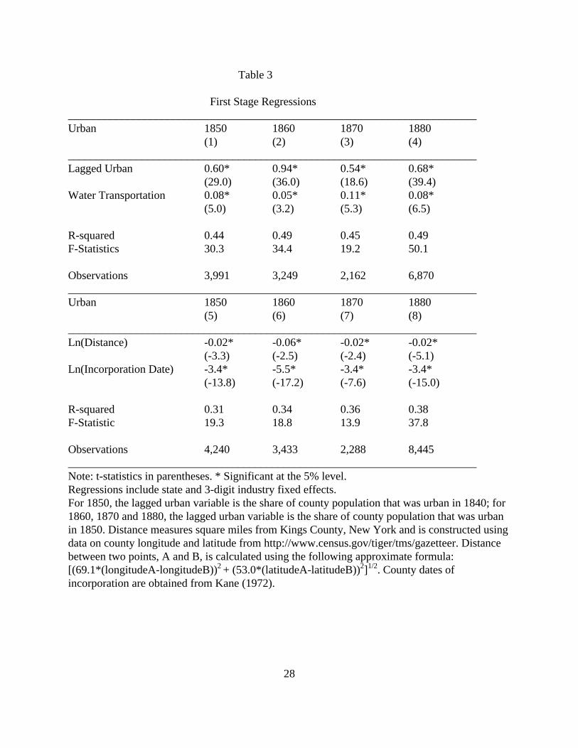
Table 3 reports the first-stage regressions of whether a firm resided in an urban or a rural
location on the instruments lagged urban variable, a dummy variable for access to water
13 The data censoring restrictions had the largest impact for the data sample in 1880. In that year, a large number of small firms located in rural areas were excluded from the sample. When the regressions were run without any censoring restrictions, the urban wage premium was higher than that reported for 1880. Note that since the regression is in semilogarithmic form, the percentage effect of the dummy variable is equal to 100(exp(a1) - 1).
14
transportation, logarithm of distance from the eastern seaboard and logarithm of dates of
incorporation.14 All of these variables are significantly correlated with the urban variable in the
expected manner. The lagged urban variable and access to water transportation were both
positively correlated with whether a firm was likely to locate in cities; firms in younger counties
and counties further from the eastern seaboard were less likely to locate in cities.
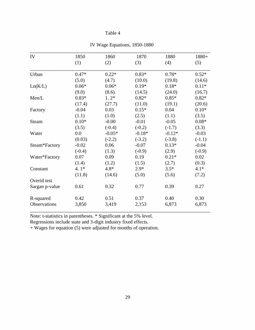
The IV regression estimates reported in Table 4 indicate that the OLS estimates of the
urban wage premium are likely to be biased downwards. The IV regression estimates show that
workers of urban firms earned 60%, 25%, 129%, and 118% higher wages than those of rural
firms for 1850, 1860, 1870 and 1880 respectively.15 In general, the IV estimates were
significantly higher than those of the OLS estimates. Since there is more than one instrument, it
is possible to test the overidentifying restrictions. In general, different combinations of any two
of the instruments, such as lagged urban and access to water or distance and date of
incorporation, exhibited the highest Sargan p-value indicating that the instruments were
uncorrelated with the structural error term. The IV regressions were least successful from the
perspective of the overidentifying restriction test when all four instruments were used. The IV
regression estimates reported were chosen for their highest Sargan p-values but the coefficients
were generally robust to different sets of instruments.
The data show that capital intensity was positively correlated with wages as expected. For
14 Distance from the eastern seaboard measures distance in square miles from Kings County, New York; the measure is constructed using data on county longitude and latitude from http://www.census.gov/tiger/tms/gazetteer. The distance between two points, A and B, is calculated using the following approximate formula: [(69.1*(longitudeA-longitudeB))2 + (53.0*(latitudeA-latitudeB))2]1/2. County dates of incorporation are obtained from Kane (1972). 15 The IV regressions use state rather than county fixed-effects. When county fixed-effects were used, the IV regressions were not identified. When the OLS regressions were run separately for county and state fixed-effects, the urban premium with county fixed-effects were generally smaller. Thus, IV estimates of the urban wage premium are likely to decline somewhat if finer geographic controls are used.
15
the capital intensity variable, the OLS and IV regression estimates are very similar. In 1850 and
1860, a percentage increase in capital intensity increased wages by 6%, but the figures rose to
18% and 19% in 1870 and 1880. However, the estimates for 1880 decline markedly when wages
are adjusted for months of operation. Thus, capital-intensive firms were more likely to operate
fulltime than labor intensive firms. The regressions also indicate that firms with a higher share of
male workers paid higher average wages.
The IV regressions indicate that firms which utilized male workers more intensely were
likely to exhibit higher average wages. Workers in water-powered artisanal firms earned less
wages than the omitted category of hand-powered, artisanal firms. On the other hand, water-
powered factory workers earned between 7% to 23% higher wages than workers in the omitted
category. The human-powered factory variable was positively significant only for 1870; the
steam and steam-powered factory variable exhibited little systematic patterns over time.
The IV regression estimates on labor productivity reported in Table 5 show that urban
workers were significantly more productive than rural workers. The labor productivity of urban
firms were 48% to 134% higher than those of rural firms between 1850 and 1880. As with
wages, labor productivity was also positively correlated with capital and male labor intensities.
The remaining variables did not exhibit systematic patterns over time. The IV regression
estimates on total factor productivity reported in Table 6 show that urban firms were 32% to
180% more productive that rural firms.16 Like the wage and labor productivity regressions, total
16 Total factor productivity estimates must be interpreted with caution. There are two potential reasons for why total factor productivity estimates may be unreliable. One major reason is that the neoclassical assumptions used to estimate total factor productivity is unlikely to hold if spatial externalities are important. In the neoclassical model, labor productivity in a simple two factor Cobb-Douglas production function (Y=AKa L1-a) can be expressed as follows: Y/L = A (K/L) a. Thus, labor productivity is equal to total factor productivity (A) times some proportion of capital intensity. However, if there are spatial external economies, then the relationship between labor and total
16
factor productivity was positively correlated with capital and male intensities. However, unlike
labor productivity, total factor productivity was also consistently positively correlated with
human-powered factory and steam variables.
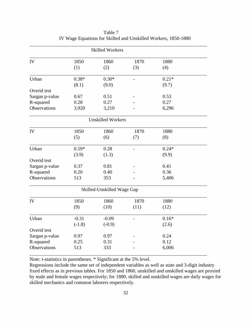
Regression estimates on the urban wage premia of skilled and unskilled workers reported
in Table 7 show that the urban wage premium appears to apply across the board for different
skilled categories. Skilled and unskilled wages, for the years 1850 and 1860, are proxied by male
and female annual wages respectively; for 1880, the skilled and unskilled wages are daily wages
for a skilled mechanic and common laborer respectively. Sample sizes of these regressions are
smaller because not all firms reported data on these variables. Table 7 shows that urban male
wages were 46% and 35% higher than rural male wages in 1850 and 1860 respectively; in 1880,
the estimated urban wage premium for a skilled mechanic was 23%. Table 8 shows that urban
female wages were 80% and 32% higher than rural female wages respectively; in 1880, urban
common laborers earned 27% higher wages than rural common laborers.
Table 7 also reports regression results on the male-female wage gap for 1850 and 1860
and the skilled-unskilled wage gap for 1880. Because the samples for these regressions were
restricted to firms which reported both skilled and unskilled wages, the regressions control for
firm specific effects which might influence the skilled-unskilled wage gap. Urbanization
generally seems to have reduced the skilled-unskilled wage gap in 1850 and 1860, but the
coefficient was only weakly significant for 1860. In 1860, the female-male wage gap in urban
factor productivity is more complex. As shown in Ciccone (2002), average labor productivity of a given region can be expressed as total factor productivity multiplied by some proportion of capital intensity and the factor responsible for spatial externalities. The second important reason may be that the OLS estimates of the neoclassical production function used to calculate total factor productivity are biased since firms with higher productivity shocks may use more inputs (see Olley and Pakes (1996) and Levinsohn and Petrin (2003)). To the extent that firms in urban areas are more likely to experience productivity shocks, the estimates of total factor productivity of urban firms may be
17
areas were 36% lower than in rural places. However, the skilled-unskilled wage gap seems to
have widened in urban areas in 1880. In that year, urban location increased the wage gap of
skilled mechanics and unskilled common laborers by 17%. Other factors that seems to have
reduced the wage gap was the intensive use of male workers and the use of water-power in
factories.
Table 8 reports urban wage, labor and total factor productivities premiums for four
alternative measures of urban agglomeration: (1) the share of population in cities with
populations of 2,500 or more, (2) the share of population in cities with populations of 8,500 or
more, (3) the total county population, and (4) the county population density. The IV regression
estimates indicate that there was a significant correlation between wages and productivity for all
these different measures of urban agglomeration. While not reported, the regressions all contain
the same set of independent variables and instruments.
The pooled difference-in-difference regression estimates reported in Table 9, based on
pooled data for all years between 1850 and 1880, indicate that urban wage and labor productivity
premiums increased significantly over this period. According to the IV estimates, the urban wage
premium remained constant between 1850 and 1860, but rose significantly in the two succeeding
decades. Relative to 1850, the omitted year, wages of workers in urban firms rose 28 to 35% and
labor productivity urban firms rose between 6 to 11% in 1870 and 1880. For the wage regression,
year dummies were positively significant for 1860 and 1870, but negatively so for 1880. For the
labor productivity, year dummies were positively significant for all years. For the pooled
regression, capital and male intensities, steam and water-powered factory variables were
biased upwards.
18
positively correlated with wages and labor productivity; steam and water-powered non-factory
variables were negatively correlated.
IV. Division of Labor and Matching Economies
The analysis of the firm-level data from the manuscript censuses for the period between
1850 and 1880 demonstrates that urban firms enjoyed significant urban agglomeration economies
and that these economies are likely to have increased over time. Evidence indicates that urban
firms were significantly more productive than rural firms and, as a result, compensated their
workers accordingly. However, the fact that wages, labor and total factor productivities were
higher for urban firms provides little guidance as to which types of urban agglomeration
economies, sharing, matching or learning economies, caused firms and workers to choose urban
locations during this phase of the industrial revolution. This section provides a discussion of the
potential causal linkages of industrialization and urbanization.
The fact that early industrialization began in rural areas of New England casts some doubt
on the importance of certain types of agglomeration economies such as sharing or learning. If
these economies were at work during early industrialization, then the early factories should have
located in major cities like New York and Boston rather than in rural townships of Dudley and
Oxford, Massachusetts.17 In particular, explanations based on variety and market sizes,
indivisibility of facilities, and access to intermediate inputs seem inconsistent with the rural
beginnings of industrialization. Moreover, geographic evidence on patents for the early and late
industrial period suggests that technological learning or spillovers may have caused patent
17 Since supplies of capital and labor are both likely to be more favorable in cities rather than in the rural countryside, Pred’s (1966) thesis that early industrialization did not start in large mercantile cities because these places lacked capital and labor seems rather suspect. Prude (1983), Hirsch (1978), Faler (1981) and Ware (1931) provide useful historical accounts of early industrialization in rural New England.
19
activity to concentrate in cities, but may not have had a similar impact on production. In general,
there seems to be little evidence that inventive and production activities were spatially correlated
during this period.18
While it is extremely difficult to empirically distinguish between the various causes of
urban agglomeration during late industrialization, a variety of evidence points toward the
importance of division of labor and matching economies.19 Indeed, the two salient features of
industrialization are the rise of the division of labor and the rise of a labor market. Prior to
industrialization, self-employed master craftsmen or artisans made the entire product using their
hand tools and learned all production techniques in apprenticeship. With industrialization,
factory owners recruited workers for a wage in the labor market and reduced their jobs into a
myriad of tasks that needed modest training to master. Because most jobs were obtained through
a network of family, friends, and people of similar ethnicity, job search costs were likely to be
significantly lower with the urban concentration of workers and firms.
The fact that industrialization first began in rural locations and then moved to cities
seems more consistent with explanations based on division of labor and matching. In early
industrialization, firms located in rural New England because early factories made extensive use
18 Lamoreaux and Sokoloff (2000) find that inventive and production activities in the glass industry were geographically concentrated in different areas. Sutthiphisal (2005) finds similar geographic patterns for a number of low- and high-tech industries between 1870 and 1910. 19 Duranton (1988) demonstrates that the agglomeration of the labor force in cities deepens division of labor between workers and raises their productivity. However, the rise of division of labor within and across firms and industries is likely to significantly increase the heterogeneity of the labor market. When specialized firms and workers must search and match for production, Kim (1989, 1990) and Helseley and Strange (1990) show that urban agglomeration raises productivity by improving the average quality of matches of firms and workers. Thus, division of labor is likely to be limited by the extent of labor market matching economies. The importance of the division of labor for growth and development has also been explored by Baumgardner (1988), Becker and Murphy (1992), and Acemoglu (1996) among others.
20
of rural native women and children.20 Because early industrialization was concentrated in only a
handful of industries, and because the division of labor was only modest, labor market
transactions costs were also likely to have been modest.21 Anecdotal evidence suggests that labor
market information was easily communicated throughout rural New England because factory
towns and cities were very specialized. For example, according to Ware (1931), the well known
Slater Mill or mills in Lowell rarely needed to advertise for help since sufficient numbers of
families and single women came to their factories seeking employment.22
In the second half of the nineteenth century, as division of labor within firms and across
industries became more extensive, and as factory production spread to numerous industries,
industrialization became a distinctly urban phenomenon. With industrialization, the occupational
categories of workers as well as the number of industries in manufacturing rose dramatically. In
1820, U.S. census officials only reported occupations by broad sectoral categories such as
agriculture, manufacturing, trade, etc. However, as occupations proliferated with
industrialization, the censuses began reporting these categories in great detail. In 1850 and 1860,
the censuses reported occupation data for 323 and 584 categories, respectively (Edwards (1943)).
20 See Goldin and Sokoloff (1984). 21 Sokoloff (1984) finds that the shift in production from artisans to non-mechanized factories, with only a modest increase in the size of the work force, was associated with significant gains in productivity. Sokoloff attributes these gains to the division of labor, especially among the relatively unskilled workers composed of women and children. 22 Ware (1931, p.212): “The use of advertising to secure help does not appear to have been wholly successful or necessary, to judge from the experience of the only mill whose advertisements could be compared with additions to the labor force. Between 1818 and 1825 only one of the Slater’s six advertisements appears to have brought desired response while another secured a quarter of the help which it called for. Twenty-three of the twenty-six families who entered his employ during this period seem to have come unsolicited. When he opened a new thread mill in 1828, however, he was successful in using this means for additional hands. Except when a sudden increase in labor force was needed, most workers probably drifted in with the growth of towns around the mills or came through chance knowledge that there might be employment available.... The boarding house mills, on the other hand, did not have to let people know that work was available. If we are to believe the tales in the Lowell Offerings, there never was any lack of employment at Lowell. Girls came from long distances unheralded, selected a boarding house, perhaps where a friend from the same village lived, and the next morning found work in the mill, usually in the same room with her friend.”
21
In addition, the census of manufactures indicate that the number of manufacturing industries rose
markedly. Although it is difficult to compare industries over time since the level of industry
aggregation differed over time, there may have been as many as 40-50 very finely defined
industries in 1820 whereas the number of industries rose to 261 and 631 in 1850 and 1860,
respectively.
There are many reasons to believe that labor market transactions costs rose significantly in
the second half of the nineteenth century. As the scale of factories rose with greater utilization of
the division of labor, and as firm and labor specialization increased, it became increasingly more
difficult to recruit and efficiently match workers and firms in rural locations. As immigration
increased significantly over the second half of the twentieth century, manufacturers shifted their
labor force from native women and children to immigrant workers who favored urban locations.
Since the most important source of labor market information came from a close network of
family and friends, firms and workers found it more effective to locate in cities where such
networks could be extended.23 Because there were considerable turnover and instability in the job
market during the period of the second industrial revolution, cities lowered the search costs of
workers in a variety of ways.24
There seems to be substantial anecdotal evidence that division of labor and labor
matching costs rose as factories increased in scale and became more mechanized. One such
example comes from the meat packing industry. While meat packing factory workers generally
possessed less skill than a traditional artisan butcher, division of labor based on skill, ability, and
23 See Nelson (1995) and Rosenbloom (2002). 24 Prude (1983) finds that the mean turnover rate at the Slater textile mill between 1813 to the mid-1830s was about 163%. He also finds that over half of the workers chose to depart voluntarily. Slichter (1919) provides additional evidence for the extremely high turnover rate of industrial workers.
22
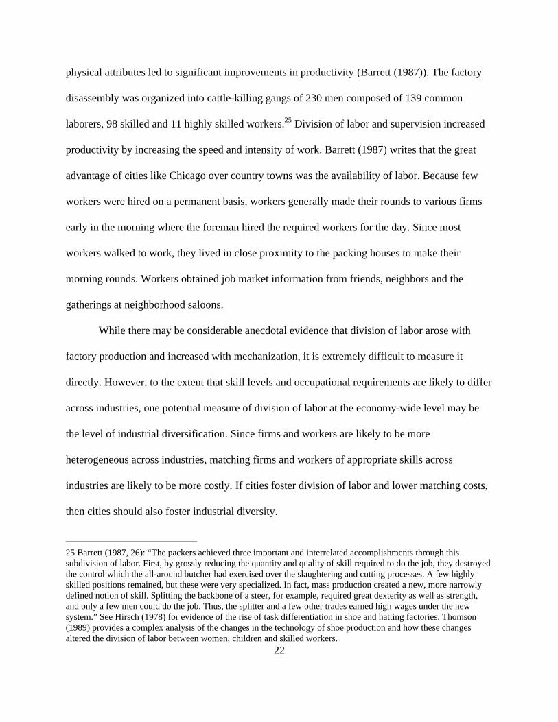
physical attributes led to significant improvements in productivity (Barrett (1987)). The factory
disassembly was organized into cattle-killing gangs of 230 men composed of 139 common
laborers, 98 skilled and 11 highly skilled workers.25 Division of labor and supervision increased
productivity by increasing the speed and intensity of work. Barrett (1987) writes that the great
advantage of cities like Chicago over country towns was the availability of labor. Because few
workers were hired on a permanent basis, workers generally made their rounds to various firms
early in the morning where the foreman hired the required workers for the day. Since most
workers walked to work, they lived in close proximity to the packing houses to make their
morning rounds. Workers obtained job market information from friends, neighbors and the
gatherings at neighborhood saloons.
While there may be considerable anecdotal evidence that division of labor arose with
factory production and increased with mechanization, it is extremely difficult to measure it
directly. However, to the extent that skill levels and occupational requirements are likely to differ
across industries, one potential measure of division of labor at the economy-wide level may be
the level of industrial diversification. Since firms and workers are likely to be more
heterogeneous across industries, matching firms and workers of appropriate skills across
industries are likely to be more costly. If cities foster division of labor and lower matching costs,
then cities should also foster industrial diversity.
25 Barrett (1987, 26): “The packers achieved three important and interrelated accomplishments through this subdivision of labor. First, by grossly reducing the quantity and quality of skill required to do the job, they destroyed the control which the all-around butcher had exercised over the slaughtering and cutting processes. A few highly skilled positions remained, but these were very specialized. In fact, mass production created a new, more narrowly defined notion of skill. Splitting the backbone of a steer, for example, required great dexterity as well as strength, and only a few men could do the job. Thus, the splitter and a few other trades earned high wages under the new system.” See Hirsch (1978) for evidence of the rise of task differentiation in shoe and hatting factories. Thomson (1989) provides a complex analysis of the changes in the technology of shoe production and how these changes altered the division of labor between women, children and skilled workers.
23
Following Duranton and Jayet (2005), industrial diversity is measured using the following
index: DI=1/Si (Eij/Ej)2 where Eij is employment in industry i in city j, Ej is total employment in
city j.26 Since data at the industry level are available only for the largest cities, the diversity
measure is constructed for 40 and 99 cities in 1860 and 1880, respectively. Because the standard
industrial codes were not devised until the mid-twentieth century, the data reported by the census
officials were at the level of product categories that perhaps resemble the current three- or four-
digit categories. In both of these years, the census officials reported information for close to 400
industries. Table 10 reports the descriptive information on these cities.
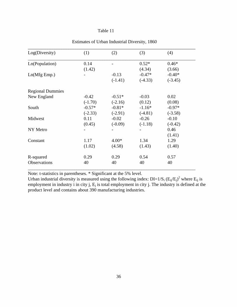
Tables 11 and 12 report regressions of the log of urban industrial diversity on the log of
total urban population and manufacturing employment; the regressions also include regional
dummy variables where the omitted region is the Middle Atlantic. The regressions show that
industrial diversity was positively and significantly correlated with urban population for both
1860 and 1880. According the specification (4), which also includes total manufacturing
employment, a percentage increase in population increased industrial diversity by 46% and 72%
in 1860 and 1880, respectively.
The regressions show that manufacturing employment was negatively correlated with
industrial diversification, especially when the regressions control for population. One
interpretation is that manufacturing employment and population are collinear. However, it is
instructive to note that large manufacturing cities which were highly specialized were
concentrated in New England. It appears that early factory towns in New England which grew
into large cities over time remained very specialized in those early industries. Since a labor force
26 Duranton and Jayet (2005) examine whether division of labor is related to city size for French cities in 1990. They find that scarce occupations, as predicted by their model, were over-represented in larger cities suggesting that
24
specialized in few industries is unlikely to possess diverse occupational skills, it is not surprising
that large industrial cities in New England were incapable of fostering industrial diversity.
V. Conclusion
Industrial revolution in the United States, as in England and other parts of Europe,
occurred in two stages. Industrialization first began in rural New England between 1820 and
1840 as the artisanal method gave way to factory organization of production in a handful
industries. However, between 1850 and 1920, as industrial revolution deepened, scale economies
rose, factory organization spread to numerous industries and regions, and industrialization
became significantly concentrated in urban areas throughout the northern region of the U.S. This
paper examines the potential causal linkages in U.S. industrialization and urbanization.
This paper finds that, at least for the period between 1850 and 1880 for which firm level
data from the manuscript censuses of manufactures are available, industrialization caused
urbanization because there were significant urban agglomeration economies. The data show that
urban firms were more productive, paid higher wages to their workers, and that urban premiums
in wages and productivity increased over time. The urban wage premium accrued to both skilled
(male) and unskilled (female) workers throughout the entire period. The urban skilled-unskilled
wage gap seems to have narrowed in 1850 and 1860, but may have widened in 1880. As
expected, other firm-level characteristics such as capital-intensity and skill-intensity (male labor
intensity) were also associated with higher wages and productivity. When the data were pooled
over the entire period, those workers who worked in water and steam-powered factories also
tended to earn higher wages when controlling for all other factors.
division of labor increased with the extent of the market.
25
While it is difficult to rule out the importance of other types of agglomeration economies
such as spillovers, this paper suggests that the geographic patterns of the two phases of
industrialization are most consistent with explanations based on division of labor and labor
market transactions cost. Because division of labor and labor matching costs were relatively
limited in early industrialization, early factories who located near rural townships in New
England did not face high costs of recruiting labor. However, in the second phase of
industrialization, as scale economies rose and as factory organization of production spread to
hundreds of industries, division of labor and matching costs rose and firms and workers became
concentrated in cities. Evidence suggests that cities with higher population levels fostered greater
industrial diversity.
Whereas workers of early factories in rural New England were composed of native
women and children, the industrial workforce of the second industrial revolution was composed
of immigrant workers. Over the century of the industrial revolution, immigrants and “birds of
passage” came to the United States in extraordinary numbers from varying European nations and
became the dominant industrial labor force. Because the extent of division of labor of the native
labor force was likely to have been limited during this period, immigrants from numerous
different nations with varying skills and physical attributes are likely to have significantly
increased the extent of division of labor available in society. Thus, immigrants who came during
the industrial period are likely to have contributed significantly to sustaining the industrial
revolution. Moreover, because division of labor is likely to have operated along ethnic lines, it is
not surprising that ethnic communities formed in cities to lower labor market transactions costs.
26
Table 1 Summary Statistics: Manuscript Censuses, 1850-1880 (mean values) __________________________________________________________________ All Firms 1850 1860 1870 1880 __________________________________________________________________ Annual Wage (Log) 5.15 5.27 5.52 5.23 Rural 5.07 5.19 5.35 4.94 Urban 5.40 5.48 5.89 5.57 Labor Productivity (Log) 5.76 6.00 6.38 6.11 Rural 5.67 5.91 6.25 5.89 Urban 6.04 6.24 6.65 6.36 Urban 0.25 0.28 0.31 0.46 Log K/L ratio 5.62 5.97 6.20 5.99 Share of Male Labor 0.67 0.68 0.68 0.69 Factory 0.10 0.10 0.15 0.16 Steam Power 0.09 0.20 0.29 0.25 Water Power 0.30 0.18 0.15 0.16 Steam*Factory 0.03 0.03 0.09 0.09 Water*Factory 0.02 0.01 0.01 0.01 Number of Firms 4,333 3,550 2,289 8,658 __________________________________________________________________ Note: Urban =1 if establishment was located in an incorporated town or city of population of 2,500 or more. Factory=1 if an establishment employed more than 15 employees. Sample selection criteria was same as that of Atack, Bateman and Margo (2004): Gross output greater than $500; for 1850 and 1860, average monthly wage greater than $4.76 but less than $190.5; and, for 1870 and 1880, average monthly wage greater than $5.20 but less than $208. Source: See Atack and Bateman (1999).
Table 3 First Stage Regressions ________________________________________________________________________ Urban 1850 1860 1870 1880 (1) (2) (3) (4) ________________________________________________________________________ Lagged Urban 0.60* 0.94* 0.54* 0.68* (29.0) (36.0) (18.6) (39.4) Water Transportation 0.08* 0.05* 0.11* 0.08* (5.0) (3.2) (5.3) (6.5) R-squared 0.44 0.49 0.45 0.49 F-Statistics 30.3 34.4 19.2 50.1 Observations 3,991 3,249 2,162 6,870 ________________________________________________________________________ Urban 1850 1860 1870 1880 (5) (6) (7) (8) ________________________________________________________________________ Ln(Distance) -0.02* -0.06* -0.02* -0.02* (-3.3) (-2.5) (-2.4) (-5.1) Ln(Incorporation Date) -3.4* -5.5* -3.4* -3.4* (-13.8) (-17.2) (-7.6) (-15.0) R-squared 0.31 0.34 0.36 0.38 F-Statistic 19.3 18.8 13.9 37.8 Observations 4,240 3,433 2,288 8,445 ________________________________________________________________________ Note: t-statistics in parentheses. * Significant at the 5% level. Regressions include state and 3-digit industry fixed effects. For 1850, the lagged urban variable is the share of county population that was urban in 1840; for 1860, 1870 and 1880, the lagged urban variable is the share of county population that was urban in 1850. Distance measures square miles from Kings County, New York and is constructed using data on county longitude and latitude from http://www.census.gov/tiger/tms/gazetteer. Distance between two points, A and B, is calculated using the following approximate formula: [(69.1*(longitudeA-longitudeB))2 + (53.0*(latitudeA-latitudeB))2]1/2. County dates of incorporation are obtained from Kane (1972).
Table 10 Industrial Diversity of Cities, 1860-1880 Summary Statistics __________________________________________________________________ 1860 1880 __________________________________________________________________ Mean SD Mean SD __________________________________________________________________ Industrial Diversity 15.08 (8.52) 9.84 (6.82) Population 96,382 (153,272) 91,717 (167,595) Manufacturing 14,945 (20,890) 12,972 (30,409) Employment Number of Cities 40 99 __________________________________________________________________ Sources: Census of Manufactures, 1860, 1880; Census of Population, 1860, 1880. Urban industrial diversity is measured using the following index: DI=1/Si (Eij/Ej)2 where Eij is employment in industry i in city j, Ej is total employment in city j. The industry is defined at the product level and contains about 390 manufacturing industries.
36
Table 11 Estimates of Urban Industrial Diversity, 1860 ________________________________________________________________________ Log(Diversity) (1) (2) (3) (4) ________________________________________________________________________ Ln(Population) 0.14 - 0.52* 0.46* (1.42) (4.34) (3.66) Ln(Mfg Emp.) - -0.13 -0.47* -0.40* (-1.41) (-4.33) (-3.45) Regional Dummies New England -0.42 -0.51* -0.03 0.02 (-1.70) (-2.16) (0.12) (0.08) South -0.57* -0.81* -1.16* -0.97* (-2.33) (-2.91) (-4.81) (-3.58) Midwest 0.11 -0.02 -0.26 -0.10 (0.45) (-0.09) (-1.18) (-0.42) NY Metro - - - 0.46 (1.41) Constant 1.17 4.00* 1.34 1.29 (1.02) (4.58) (1.43) (1.40) R-squared 0.29 0.29 0.54 0.57 Observations 40 40 40 40 ________________________________________________________________________ Note: t-statistics in parentheses. * Significant at the 5% level. Urban industrial diversity is measured using the following index: DI=1/Si (Eij/Ej)2 where Eij is employment in industry i in city j, Ej is total employment in city j. The industry is defined at the product level and contains about 390 manufacturing industries.
37
Table 12 Estimates of Urban Industrial Diversity, 1880 ________________________________________________________________________ Log(Diversity) (1) (2) (3) (4) ________________________________________________________________________ Ln(Population) 0.44* - 0.77* 0.72* (6.88) (6.31) (5.76) Ln(Mfg Emp.) - 0.19* -0.26* -0.24* (3.90) (-3.10) (-2.86) Regional Dummies New England -0.28 -0.44* -0.16 -0.12 (-1.64) (-2.28) (-0.96) (-0.72) South 0.05 0.08 -0.06 -0.01 (0.31) (0.39) (-0.39) (-0.04) Midwest 0.47* 0.45* 0.46* 0.51* (3.05) (2.55) (3.05) (3.36) West 0.52 0.60 0.32 0.38 (1.87) (1.86) (1.16) (1.39) NY Metro - - - 0.56 (1.61) Constant -2.85* 0.34 -4.19* -3.86* (-3.85) (0.75) (-5.17) (-4.67) R-squared 0.44 0.27 0.49 0.51 Observations 99 99 99 99 ________________________________________________________________________ Note: t-statistics in parentheses. * Significant at the 5% level. Urban industrial diversity is measured using the following index: DI=1/Si (Eij/Ej)2 where Eij is employment in industry i in city j, Ej is total employment in city j. The industry is defined at the product level and contains about 390 manufacturing industries.
38
References Abdel-Rahman, H. and M. Fujita. 1990. “Product Variety, Marshallian Externalities, and City Sizes,” Journal of Regional Science 30 (2): 165-183. Acemoglu, Daron. 1996. “A Microfoundation for Social Increasing Returns in Human Capital Accumulation,” Quarterly Journal of Economics 111: 779-804. Atack, Jeremy and Fred Bateman. 1999. "U.S. Historical Statistics: Nineteenth-Century U.S. Industrial Development through the Eyes of the Census of Manufactures," Historical Methods 32 (4): 177-188. Atack, Jeremy, Fred Bateman and Robert Margo. 2004. “Skill Intensity and Rising Wage Dispersion in Nineteenth-Century American Manufacturing,” Journal of Economic History 64 (1): 172-192. Barrett, James R. 1987. Work and Community in the Jungle: Chicago’s Packinghouse Workers 1894-1922. University of Illinois Press. Baumgardner, J.R. 1988. “The Division of Labor, Local Markets and Worker Organization,” Journal of Political Economy 96 (3): 509-527. Becker, Gary S. and Kevin M. Murphy. 1992. “Division of Labor, Coordination Costs, and Knowledge,” Quarterly Journal of Economics 107 (4): 1137-1160. Berliant, Marcus and Ping Wang. 1993. “Endogenous Formation of a City Without Agglomerative Externalities or Market Imperfections: Marketplaces in a Regional Economy,” Regional Science and Urban Economics 23 (1): 121-144. Buchanan, J.M. 1965. “An Economic Theory of Clubs,” Economica 32 (125):1-14. Ciccone, Antonio. 2002. “Agglomeration-Effects in Europe,” European Economic Review 46 (2): 213-227. Ciccone, Antonio and Robert E. Hall. 1996. “Productivity and the Density of Economic Activity,” American Economic Review 86 (1): 54-70. Ciccone, Antonio and Giovanni Peri. 2004. “Identifying Human Capital Externalities: Theory with Applications,” mimeo. Duranton, Gilles. 1998. “Labor Specialization, Transport Costs and City Size,” Journal of Regional Science 38: 553-573. Duranton, Gilles and Diego Puga. 2001. “Nursery Cities: Urban Diversity, Process Innovation, and the Life Cycle of Products,” American Economic Review 91 (5): 1454-1477. Duranton, Gilles and Diego Puga. 2004. “Micro-foundations of Urban Agglomeration Economies,” in Handbook of Regional and Urban Economics, Volume 4, J.V. Henderson and J. Thisse, eds., Elsevier. Duranton, Gilles and Jubert Jayet. 2005. “Is Division of Labour Limited by the Extent of the Market? Evidence from French Cities,” mimeo. Edwards, Alba M. 1943. Comparative Occupation Statistics for the United States, 1870 to 1940. U.S. Bureau of the Census. Faler, Paul G. 1981. Mechanics and Manufacturers in the Early Industrial Revolution: Lynn, Massachusetts, 1780-1860. SUNY Press. Glaeser, Edward L. 1999. “Learning in Cities,” Journal of Urban Economics 46 (2): 254-277. Glaeser, Edward L. 2005. “Reinventing Boston: 1630-2003,” Journal of Economic Geography 5: 119-153.
39
Glaeser, Edward L. and David C. Mare. 2001. “Cities and Skills,” Journal of Labor Economics 19 (2): 316-342. Goldin, Claudia and Kenneth L. Sokoloff. 1984. “The Relative Productivity Hypothesis of Industrialization: The American Case, 1820-1850.” Quarterly Journal of Economics 99: 461-488. Helsley, Robert W. and William C. Strange. 1990. “Matching and Agglomeration Economies in a System of Cities,” Regional Science and Urban Economics 20: 189-212. Hirsch, Susan E. 1978. Roots of the American Working Class: The Industrialization of Crafts in Newark, 1800-1860. University of Pennsylvania Press. Hunter, Louis C. 1985. A History of Industrial Power in the United States: Steam Power, volume 2. University of Virginia Press. Jovanovic, B. and R. Rob. 1989. “The Growth and Diffusion of Knowledge,” Review of Economic Studies 56 (4): 569-582. Kane, Joseph Nathan. 1972. The American Counties. Third Edition. Scarecrow Press. Kim, Sukkoo. 2000. “Urban Development in the United States, 1690-1990,” Southern Economic Journal 66 (4): 855-880. Kim, Sukkoo. 2005. “Industrialization and Urbanization: Did the Steam Engine Contribute to the Growth of Cities in the United States?” Explorations in Economic History 42 (4): 586- 598. Kim, Sukkoo and Robert Margo. 2004. “Historical Perspectives on U.S. Economic Geography,” in Handbook of Regional and Urban Economics, Volume 4, Vernon Henderson and Jacques-Françoise Thisse, eds., North-Holland/Elsevier. Kim, Sunwoong. 1989. “Labor Market Specialization and the Extent of the Market,” Journal of Political Economy 97 (3): 692-705. Kim, Sunwoong. 1990. “Labor Heterogeneity, Wage Bargaining, and Agglomeration Economies,” Journal of Urban Economics 28: 160-177. Lamoreaux, Naomi R. and Kenneth L. Sokoloff. 2000. “Location and Technological Change in the American Glass Industry During the Late Nineteenth and Early Twentieth Centuries,” Journal of Economic History 60: 700-729. Levinsohn, James and Amil Petrin. 2003. “Estimating Production Functions Using Inputs to Control For Unobservables,” Review of Economic Studies 70 (2): 317-342. Moretti, Enrico. 2004. “Human Capital Externalities in Cities,” in J.V. Henderson and J.F. Thisse (Eds.), Handbook of Regional and Urban Economics, vol. 4. North-Holland. Nelson, Daniel. 1995. Managers and Workers: Origins of the Twentieth Century Factory System in the United States 1880-1920. University of Wisconsin Press. Olley, G. Steven and Ariel Pakes. 1996. “The Dynamics of Productivity in the Telecommunications Equipment Industry,” Econometrica 64 (4): 1263-1297. Palivos, T. and P. Wang. 1996. “Spatial Agglomeration and Endogenous Growth,” Regional Science and Urban Economics 26 (6): 645-669. Pred, Allan R. 1966. The Spatial Dynamics of U.S. Urban-Industrial Growth, 1800-1914. MIT Press. Prude, Jonathan. 1983. The Coming of Industrial Order: Town and Factory in Rural Massachusetts 1810-1860. Cambridge University Press. Rosenberg, Nathan and Manuel Trajtenberg. 2004. “A General Purpose Technology at Work:
40
The Corliss Steam Engine in the Late-Nineteenth-Century United States,” Journal of Economic History 64 (1): 61-99. Rosenbloom, Joshua L. 2002. Looking For Work, Searching For Workers. Cambridge University Press. Slichter, Sumner H. 1919. The Turnover of Factory Labor. D. Appleton and Co. Sokoloff, Kenneth L. 1984. “Was the Transition from the Artisanal Shop to the Nonmechanized Factory Associated with Gains in Efficiency?: Evidence from the U.S. Manufacturing Censuses of 1820 and 1850,” Explorations in Economic History 21: 351-382. Sutthiphisal, Dhanoos. 2005. “The Geography of Invention in High- and Low-Technology Industries: Evidence from the Second Industrial Revolution,” mimeo. Thomson, Ross. 1989. The Path to Mechanized Shoe Production in the United States. University of North Carolina Press. Ware, Caroline F. 1931. The Early New England Cotton Manufacture. Houghton Mifflin Company. Wheaton, William C. and Mark J. Lewis. 2002. “Urban Wages and Labor Market Agglomeration,” Journal of Urban Economics 51: 542-562. Wheeler, Christopher. 2001. “Search, Sorting, and Urban Agglomeration,” Journal of Labor Economics 19 (4): 879-899. Wheeler, Christopher. 2004. “Wage Inequality and Urban Density,” Journal of Economic Geography 4: 421-437.