DRUG DIFFUSION THROUGH PEER NETWORKS:THE INFLUENCE OF INDUSTRY PAYMENTS
Leila AghaDan Zeltzer
Working Paper 26338http://www.nber.org/papers/w26338
NATIONAL BUREAU OF ECONOMIC RESEARCH1050 Massachusetts Avenue
Cambridge, MA 02138October 2019
For helpful comments and suggestions we thank Liran Einav, Erzo F.P. Luttmer, Kyle Myers, David Molitor, Jonathan Skinner, Douglas Staiger, and seminar participants at Tel Aviv University, Dartmouth College, ASHEcon, the ASSA Annual Meeting in Atlanta, the Fifth Annual Network Science and Economics Conference at Indiana University, the Barcelona GSE Summer Forum, and the NBER Summer Institute. The authors gratefully acknowledge research support by NIH grants PO1 AG19783 and UO1 AG046840. Dan Zeltzer acknowledges support from The Foerder Institute for Economic Research at Tel Aviv University. We thank Stephanie Tomlin and Weiping Zhou for help obtaining and managing the data. The content is solely the responsibility of the authors. The views expressed herein are those of the authors and do not necessarily reflect the views of the National Bureau of Economic Research.
NBER working papers are circulated for discussion and comment purposes. They have not been peer-reviewed or been subject to the review by the NBER Board of Directors that accompanies official NBER publications.
Drug Diffusion Through Peer Networks: The Influence of Industry PaymentsLeila Agha and Dan ZeltzerNBER Working Paper No. 26338October 2019JEL No. I11,O33
ABSTRACT
Pharmaceutical companies' marketing efforts primarily target physicians, often through individual detailing that entails monetary or in-kind transfers. We study how peer influence broadens these payments' reach beyond the directly paid physicians. Combining Medicare prescriptions and Open Payments data for anticoagulant drugs, we document that pharmaceutical payments target highly connected physicians. We exploit within-physician variation in payment exposure over time to estimate the payments' influence. Unlike the paid doctor, peer physicians are not directly selected by the pharmaceutical company on the basis of their expertise or enthusiasm for the target drug. Yet, following a large payment, prescriptions for the target drug increase both by the paid physician and the paid physician's peers. These peer effects influence doctors who share patients with the paid physician, even when the two doctors are not affiliated with the same group practice. We find no evidence that payments reduce prescriptions among high-risk patients. Over the period 2014--2016, physician payments associated with anticoagulant marketing increased the drugs' prescription volume by 23 percent, with peer spillovers contributing a quarter of the increase.
Dan ZeltzerThe Eitan Berglas School of EconomicsTel Aviv UniversityP.O.Box 39040Tel Aviv 6997801Israel [email protected]
A data appendix is available at http://www.nber.org/data-appendix/w26338
Introduction
Drug and medical device companies spend the majority of their promotional budgets, over
$20 billion annually, on marketing to health care providers. Much of this spending is on
face-to-face detailing efforts to encourage adoption of new clinical products. Recent evi-
dence suggests this marketing impacts prescription behavior, and an ongoing public debate
centers on the influence of drug manufacturers’ promotional efforts.1 While pharmaceutical
companies’ interactions with physicians may educate doctors about new drugs, such engage-
ment may also increase the prescribing volume of higher cost, brand name products marketed
by the industry, not necessarily in the best interests of patients or payers.2
Large detailing payments reportedly target thought leaders, i.e. physicians who may be
highly influential on the practice of their peers. Supported by a burgeoning commercial intel-
ligence industry that identifies Key Opinion Leaders in different locations and therapy areas,
pharmaceutical marketing increasingly leverages indirect influence (Campbell 2008). While
influencer marketing and viral marketing are common promotional strategies in consumer
goods markets (Iyengar et al. 2011), understanding their scope in medicine, where informa-
tion asymmetries leave a large potential for over- and under-adoption of new technologies,
is of particular policy importance. In this paper, we study how pharmaceutical detailing
payments impact drug diffusion through the peer networks of targeted doctors.
Absent experimental variation, research into peer influence faces a significant hurdle:
local clustering may be the result of common shocks or correlated preferences rather than
peer effects. To isolate peer effects from these competing explanations, we exploit within-
doctor variation in exposure to promotional payments over time. This study’s contribution
is twofold: first, it provides a lens for understanding the role of local physician networks
in technology diffusion; second, it provides a more complete accounting of the impact of
pharmaceutical companies’ promotional efforts.
To study the influence of pharmaceutical payments on prescription behavior, we use
Medicare Part D administrative claims data. We focus on prescriptions of anticoagulants
(commonly referred to as “blood thinners”), a widely used therapeutic class to which several
new drugs were introduced during or shortly before our sample period. We match prescrip-
tion data with two other data sources: (1) the universe of payments and value transfers to
US physicians by drug manufacturers and distributors, and (2) data on physician networks,
where physicians are considered connected if they share patients.
1For a recent overview of drug promotion strategies, spending levels, and impacts, see Schwartz andWoloshin (2019).
2E.g., Thomas, Katie et al., “Detailing Financial Links of Doctors and Drug Makers,” New York Times,September 30, 2014; Elliot, Carl, “The Drug Pushers,” The Atlantic, April 2016.
1
Our paper contributes to a growing body of literature investigating the effect of pharma-
ceutical marketing on prescribing decisions (David et al. 2010; DeJong et al. 2016; Larkin
et al. 2017; Shapiro 2018a; Sinkinson and Starc 2018; Grennan et al. 2018). Our empiri-
cal approach, which accounts for physician-drug fixed effects, is most similar to Carey et al.
(2015). Studying an earlier time period and a different set of drugs, Carey et al. (2015) found
that pharmaceutical payments increase the targeted doctor’s prescribing volume. Consistent
with earlier work, we find that physicians increase their own prescribing of the target drug
after a detailing interaction. Furthermore, we present new evidence that large payments
increase prescribing by peers of targeted physicians. To our knowledge, this is the first paper
to investigate the peer effects of pharmaceutical payments.
For each drug in our sample, roughly one-third of practicing physicians receive small
in-kind transfers of food and beverages (typically under $20) associated with detailing in-
teractions with marketing salespersons; we refer to these as “food payments”. In contrast,
fewer than 2 percent of physicians receive large payments associated with speaking, consult-
ing, and other services; we refer to these as “compensation payments”. Despite the vastly
lower penetration, compensation payments account for two-thirds of the total dollar vol-
ume transferred; the median of such payments is above $2,000, and most recipients receive
repeated payments for the same drug. We show that compensation payments disproportion-
ately target physicians with many peers.
After a physician receives a compensation payment, each of their peers increases use
of the target drug by 2 percent on average. This finding is shown graphically in Figure 1
and holds up within an empirical framework that accounts for physician-drug fixed effects
and allows for differential pre-trends. The framework allows for physicians who engage with
pharmaceutical companies to differ ex ante in both their baseline propensity to prescribe
and their speed of new drug adoption. The key identification assumption is that detailing
payments to a peer of the focal physician do not coincide with other shocks to the focal
physician’s demand for the new drug. One advantage of our focus on peer effects is that
we are studying payment influence on doctors who were not themselves directly targeted
or selected by the pharmaceutical company, which mitigates endogeneity concerns around
payment timing.
Peer spillover effects of compensation payments extend to physicians who share patients
but are not affiliated with the same group practice. Further, we find that the estimated peer
effects are not solely driven by prescription refills; peer influence leads to greater use of the
target drug as a first-line therapy for patients without a prior anticoagulant prescription.
Increased prescriptions due to payments do not come at the expense of competing drugs,
but reflect an expansion of the new anticoagulant drug class as a whole. In contrast to our
2
findings on large compensation payments, small food payments induce the recipient doctor
to prescribe more of the targeted drug but have no economically or statistically significant
peer spillover effects.
The indirect effect of compensation payments on each of the recipient’s peers’ prescription
volume is roughly 1/20 the size of the direct effect of the compensation payment on the paid
recipient himself and 1/3 the size of directly receiving a food payment. But while spillover
effects on each peer are smaller than the direct effect of receiving a payment, given that the
physicians targeted with these compensation payments have more than 60 peers on average,
the overall estimated impact of a compensation payment on all first-degree peers eclipses the
estimated impact of a compensation payment on the paid physician’s own patient volume.
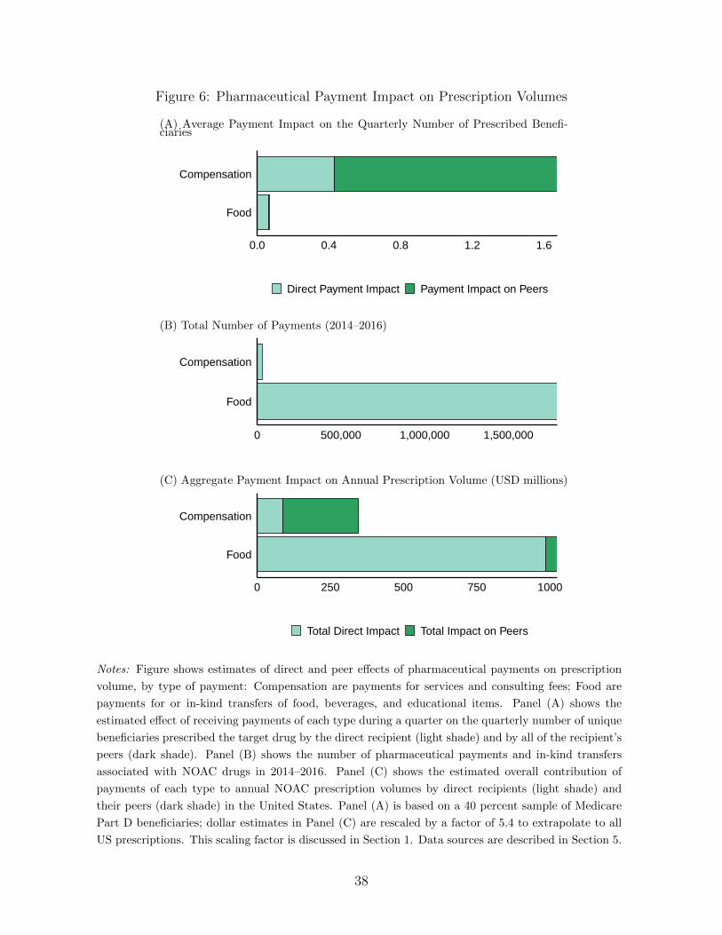
Relative to a counterfactual without pharmaceutical payments of any type, pharmaceu-
tical payments have increased New Oral Anticoagulant (NOAC) prescription volume by 23
percent over the 2014–2016 period, increasing their estimated US market size from $6.2 bil-
lion to 7.6 billion. While much of this impact is driven by the direct influence of widespread
food payments on recipient doctors, about a quarter of the increase is due to peer spillover
effects of infrequent (but very large) compensation payments. This estimate of spillovers
is conservative because it fails to account for other peer relationships besides measured
patient-sharing ties. These results, which take into account the actual network structure
and distribution of payments, imply that the impact of pharmaceutical payments on the
adoption of new drugs is substantially amplified through peer effects. This amplification
helps explain why pharmaceutical companies spend most of their promotional payments on
a small number of doctors.
Our counterfactual analysis also suggests that pharmaceutical detailing increases the
variance of drug adoption across regions. Prior research has documented significant local
clustering of treatment patterns (Cutler et al. 2019; Skinner and Staiger 2015; Moen et al.
2016; MacLeod and Currie 2018). Because payments are concentrated in areas where initial
adoption is already high, they contribute to regional divergence in prescription patterns, at
least in the intermediate stages of the drug life cycle that we observe.
The welfare implications of pharmaceutical influence are not immediately obvious. If
detailing payments propagate useful information to physicians, they could improve prescrip-
tion safety and value. Studying prescription decisions for patients with atrial fibrillation,
we find no evidence that detailing interactions increased concordance with evidence-based
clinical guidelines either among directly paid physicians or their peers.
Our findings corroborate prior evidence on the importance of peer influence in health
care decisions (Chan 2018; Navathe and David 2009; Oster and Thornton 2012; Silver 2019)
as well as in other technology adoption settings (Banerjee et al. 2013; Golub and Sadler
3
2016; Galeotti et al. 2017). Prior work suggests that peer spillovers may be successful at
increasing use of new drugs (Coleman et al. 1957; Donohue et al. 2018; Agha and Molitor
2018), but may not help curb the use of low-value or risky prescribing (Sacarny et al. 2019).
Our paper brings a new focus to this area of inquiry, showing that private firms effectively
leverage peer influence for marketing purposes.
The rest of this paper proceeds as follows. Section 1 describes the data and contextual
information about the class of anticoagulants. Section 2 describes our empirical strategy.
Section 3 shows our main estimates of the influence of pharmaceutical payments on pre-
scription volume. Section 4 analyzes whether drug detailing promotes guideline-concordant
anticoagulant use for patients with atrial fibrillation. Section 5 quantifies the impact of pay-
ments on the aggregate increase and spatial dispersion of prescription volumes. Section 6
shows estimated effects on competitors. Section 7 concludes.
1 Data and Context
Our analysis focuses on anticoagulants, studying the diffusion of three NOACs: apixaban
(brand name Eliquis), dabigatran (Pradaxa), and rivaroxaban (Xarelto). These drugs com-
prise a growing market for alternatives to the older anticoagulant, coumadin (Warfarin), as
shown in Figure 2. These three NOACs were introduced between 2010 and 2012, shortly
before our sample period began in 2014.3
Anticoagulants are primarily used to prevent strokes and other clotting events in patients
with atrial fibrillation, deep vein thrombosis, and pulmonary embolism. These conditions are
both common and serious, estimated to contribute to 240,000 deaths per year in the United
States.4 The NOAC global market was $23 billion in 2013, and is projected to double by
2025.5
NOACs are considered noninferior to existing anticoagulant drugs. Cited advantages of
NOACs relative to older anticoagulant drugs include improved safety, convenience of use,
fewer interactions with other drugs, a wider therapeutic window, and no need for laboratory
monitoring (Mekaj et al. 2015). These benefits come at a cost: NOACs were branded drugs,
3The FDA first approved Pradaxa on October 19, 2010, Xarelto on July 1, 2011, and Eliquis on December28, 2012. This slight variation in the introduction of drugs means that we have a chance to observe slightlydifferent stages in the life cycle of product introduction.
4Estimates reported by the Center for Disease Control https://www.cdc.gov/stroke/facts.htm andhttps://www.cdc.gov/ncbddd/dvt/documents/blood-clots-fact-sheet.pdf. Accessed August 2019
5Global Anticoagulants Market Expected to Reach $43 Billion By 2025. Allied Market Research Re-port. https://www.alliedmarketresearch.com/press-release/anticoagulant-drugs-market.html.Accessed August 2019.
priced at more than $500 per month—multiple times the price of off-patent Warfarin.6
1.1 Data Sources
To estimate peer effects in the diffusion of new drugs, we combine multiple databases on pre-
scriptions, payments, and connections as follows. Physician prescription volumes are derived
from Medicare Part D administrative claims, from 2014–2016. Associated payments and in-
kind transfers to physicians made by drug manufacturers are identified in the Open Payments
database, from mid-2013 until the end of 2016. Physician shared-patients relationships are
merged from the 2013 Referral Patterns database. Additional physician characteristics, in-
cluding practice location and group practice affiliations are from Physician Compare.7
Prescriptions We analyze a 40 percent sample of Research Identifiable Medicare Part D
claims in 2014–2016 (CMS 2013–2016a). To track the adoption and use of new anticoagulant
drugs, we restrict attention to physicians of medical specialties that together comprise the
majority of NOAC prescribers: primary care and cardiology.8
For each physician and each anticoagulant drug, we construct a quarterly panel of the
doctor’s prescription volume. We use this data to define three outcome variables. Our
primary outcome is the number of unique Medicare Part D beneficiaries prescribed the drug
in that quarter. Second, we construct a count of newly initiated prescriptions, excluding
prescription renewals or drug changes for patients already using anticoagulants. We define
newly prescribed patients as those who did not fill any type of anticoagulant prescription
for the prior 12 months.9 Finally, to measure the relative market share of each drug at the
physician level, we calculate the fraction of patients prescribed each specific NOAC out of
the total anticoagulant prescriptions. This relative share variable is defined only in quarters
with at least one anticoagulant prescription and therefore corresponds to a smaller sample
size (See Table 1).
6Anticoagulants - prices and information, https://www.goodrx.com/anticoagulants. Accessed September,2019.
7With the exception of the Medicare Part D Research Identifiable patient-level data, all data are publiclyavailable. All of these databases are maintained by the Centers of Medicare and Medicaid Services (CMS),a federal agency within the US Department of Health and Human Services.
8We define primary care physicians as those whose primary specialty recorded in the Physician Comparedatabase is one of: Family Practice, Internal Medicine, General Practice, or Geriatric Medicine. Cardiologistsare defined as physicians whose primary specialty is one of: Cardiology, Interventional Cardiology, or CardiacSurgery.
9For the purposes of this study, when we refer to anticoagulants as a class, we consider all prescriptionsfor Warfarin, Xarelto, Eliquis, and Pradaxa, which cover all the major prescription anticoagulants over thistime period.
5
Peers To study peer effects in prescription decisions, we combine prescription informa-
tion with physician referral data from the CMS Referral Patterns data (CMS 2013). In
these data, two physicians have a shared patient if they both participated in the delivery of
health services to the same Medicare patient within 30 days of one another. Two physicians
are defined to be peers if they have 11 or more shared Medicare Fee For Service patients
within a year. The threshold of 11 patients was chosen by CMS to protect patient pri-
vacy. But according to survey evidence, it happens to match well the number of shared
Medicare patients between two physicians above which the physicians are likely to have a
recognized professional relationship.10 Therefore peers thus defined may also influence each
other’s practice. Furthermore, a key channel for peer influence is via passively observing
peer prescription behavior for shared patients, so this definition of peer ties coincides with
a potentially important mechanism for peer effects.
We treat this network as static, undirected, and unweighted. We define peers based on the
observed network of shared-patient peers in 2013, the year before our prescription outcome
data begins, to reduce concern for endogenous responses of physician work relationships to
payments.11
Appendix Table A1 presents summary statistics on the distribution of the number of
peers. The mean physician in our sample shares patients with 22.8 peers (median 13).
Cardiac specialists, whose practice is more specialized, have significantly more peers (mean
60.2, median 53) than generalists (mean 17.1, median 11). More-experienced physicians also
tend to have more peers.
Payments We combine data on NOAC drug prescriptions with data on associated pay-
ments and value transfers to physicians by drug manufacturers and distributors from the
Open Payments database (CMS 2013–2016b). This payment data covers the period from
July 1, 2013 through December 31, 2016. This database is maintained by CMS as part of
the Physician Financial Transparency Reports (Sunshine Act), a national disclosure program
created by the Affordable Care Act. Since 2013, manufacturers have been required to submit
data about all payments and other transfers of value made to physicians (which we refer to
as payments). The reports include the amount paid (or value of nonmonetary transfer, such
10Barnett et al. (2011) find that 82 percent of physician pairs with nine patient shared report to have anadvice or referral relationship, compared with only 19 percent of physician pairs with one shared patient.Furthermore, using publicly available shared-patient data makes it easier to replicate and reuse all parts ofour analysis, except for those that use Medicare Part D confidential data. We are able to reproduce theresults using a claims-based definition of referral relationships from confidential data.
11However, responses of physician working relationships to payments are likely small. Physician workingrelationships have been shown to be persistent (Zeltzer forthcoming). Furthermore, shared-patient relation-ships are measured using all Medicare patients, not just patients with anticolagulant prescriptions.
6
as food or travel expenses), the associated drug(s), and the nature of the transfer. We match
doctors listed in Open Payments to National Provider Identifier codes based on physician
name and address.12 We aggregate payments received to construct a panel of physician
payment amounts and payment types in each quarter and for each drug.
From 2014–2016, the reported payments total to $103 million for the three NOAC drugs
we study. Table 2 shows the distribution of payment size by payment type. We group
payment types into three categories based on average payment size: (1) food, beverage,
and education; (2) consulting fees and compensation for services; (3) travel and lodging.
Figure 3 shows the average cumulative number of payments associated with each drug that
were received by physicians of different specialties. Appendix Figure A1 shows the cumulative
fraction of recipients of any payments of each type.
The most common transfers are in the form of food, beverages, and educational ma-
terials purchased by salespeople when discussing new drugs with physicians. Our sample
includes 1.8 million transfers of this nature, most of them for food and beverages. These
small payments, averaging below US$40 per payment, are received by both generalists and
specialists.
The largest category of payments by both average size per payment and total dollar
expenditure is compensation for services and consulting fees. We observe 30,000 of these
large payments, with each transaction averaging over US$2,200. As we later show, these
payments are concentrated among a small fraction of physicians, most of whom are cardiac
specialists.
Payments for travel and lodging are a third, smaller category. Our sample reports 18,000
travel transactions, accounting for only 5 percent of total detailing expenditures. Transfers
in this category are of intermediate value, averaging $260 per transaction. Consistent with
their low frequency, we generally do not have sufficient statistical power to estimate the
relationship between travel payments and prescription volume. Our results do not change if
we omit them altogether. For completeness, we control for travel payments in all regressions.
Physician characteristics Finally, we use the Physician Compare data to identify the
physician’s primary specialty, experience (measured as years since medical school gradua-
tion), and group practice affiliations. The group practice affiliations form the basis of a
second measure of physician peer links, defined as physicians who share at least one common
group practice. We use these to supplement our baseline measure of peer linkages defined
12We use Physician Compare for name and address information. As both Physician Compare and OpenPayments are maintained by CMS, more than 97 percent of our matches are exact matches on last name, firstname, and state. The remaining matches include slight misspellings; we match these remaining records byblocking on state and first letter of last name, and using fuzzy string matching with the Jaro-Winkler distance.
7
by shared patients.
1.2 Patterns of Pharmaceutical Payments, Prescriptions, and Peer
Connections
Physicians who share patients with many peer physicians are more likely to receive com-
pensation payments. Figure 4 sorts physicians by decile of number of peers (i.e., network
degree) within each hospital referral region (HRR) and specialty type; it then plots how the
average number of pharmaceutical payments per physician varies across the distribution of
peer group size. While physicians with relatively few peers are less likely to receive food
from pharmaceutical companies promoting one of our three NOACs, there is little difference
in the rate of food payment among the top four deciles of the distribution for either cardiac
specialists or primary care physicians. By contrast, highly connected physicians, in the top
deciles of the distribution of number of peers, are more likely to be targeted with compensa-
tion payments than peers with the median number of connections, a pattern we see for both
cardiac specialists and primary care physicians.
Appendix Table A2 regression results show that having a greater number of peers (i.e., a
higher network degree centrality) is associated with higher payments even after accounting
for other observed physician characteristics.13 These data are consistent with the possibility
that pharmaceutical companies target large payments to highly connected doctors, who
may be better positioned to amplify the payment’s impact. A caveat to interpreting this
relationship is that physicians with more peer connections may also see more patients in
their own practice.
Table 1 shows summary statistics by physician own and peer payment status. This table
is restricted to our analysis sample for consistency with the subsequent regression results.
Specifically, we impose two sample requirements to ensure the physician is actively treating
Medicare enrollees: first, the doctor must have at least one peer provider as defined by
the CMS Referral Patterns data; second, the physician must write at least one observed
anticoagulant prescription (for any of the anticoagulant drugs, including Warfarin) over the
three-year study period. These two restrictions together drop 17 percent of the physicians
listed in Physician Compare from our sample. We further require that physicians who receive
their first observed payment during our sample period (January 1, 2014 through December
31, 2016) have two quarters of pre-payment data and two quarters of post-payment data.
We impose this restriction for own compensation, own travel, and own food payments as
13We also studied alternative centrality measures, including eigenvector, closeness, and betweenness cen-trality. Degree centrality appears to be the most robust predictor of payments.
8
well as peer compensation payments. This restriction ensures that we have a balanced panel
for at least four quarters around the first payment event, which is important to accurately
compare doctors’ prescription volume before and after the payment.
Table 1 reports that 73 percent of doctors in our sample receive no payments directly.
On average, 27 percent of doctors receive food or travel payments for each drug, and these
doctors average $148 in payments for the target drug over the 12 quarters of our sample.
This total transfer is typically spread across several transactions: physicians receiving food
payments for a particular drug are paid in four out of 12 quarters on average. By contrast, the
0.3 percent of physicians who receive compensation payments for each drug are drawing much
larger transfers from pharmaceutical companies, averaging $38,166 per doctor cumulatively
over 12 quarters. Physicians receiving compensation payments average six quarters (out of
12) with compensation payments. Cardiac specialists constitute the majority (81.2 percent)
of recipients of compensation payments.
Even though less than one percent of doctors in our sample receive compensation pay-
ments for a given drug, these paid doctors are highly connected. Therefore, we find that
14 percent of doctors in our sample are linked to a compensation-paid physician for a given
drug. Our econometric approach relies on comparisons of physicians who are and are not
linked to compensation-paid peers to identify peer effects.
This table also illustrates that physicians directly and indirectly targeted with payments
use the target drug more intensely. Doctors whose peers receive compensation payments
prescribe each NOAC to 1.12 patients per quarter, on average, compared to 0.45 patients
per quarter for doctors whose peers do not receive compensation payments. We explore this
relationship in our regression analysis.
Note that the prescription volumes reported here cover only a modest fraction of doctors’
overall patient panel. We observe prescriptions for a 40 percent sample of Medicare Part
D enrollees. Hoadley et al. (2015) reports that 72 percent of Medicare beneficiaries were
enrolled in Part D as of 2015, suggesting our sample covers roughly 28 percent (= 0.4 ·0.7) of
Medicare beneficiaries. Further, in the 2014 Medical Expenditure Panel Survey, 66 percent
of NOAC prescriptions are written to patients 65 years or older. Thus, roughly scaling our
patient counts up to the full population requires multiplying the patient volume by a factor
of 5.4. For simplicity and because the scaling requires additional assumptions, e.g. that
the impact of pharmaceutical payments on prescribing patterns for non-Part D enrollees is
similar, we report unscaled results.
9
2 Identification and Estimation
Our analysis focuses on estimating pharmaceutical payments’ spillover effects on the peers
of targeted physicians. The main identification concern is endogeneity of peer prescriptions:
peers of paid physicians may have had higher prescription rates even in the absence of their
peer’s payment. To isolate the impact of peer payment, we begin with an event study
approach exploiting variation in the timing of payments and the peer group of targeted
physicians.
2.1 Regression models of payment impact
We model prescription decisions as a function of payments, including payments both directly
made to the physician and payments to the index doctor’s peer. We begin with a graphical
event study around the first payment exposure of each type and then move to a specification
that studies the accumulating impact of each transfer.
Let i index physicians, t index time in quarters, and d index drugs. Let Yitd denote the
prescription volume of drug d by doctor i at period t. Let G denote the network of rela-
tionships among physicians based on having common patients (see Section 1 for definitions).
That is, for each i, j, let sij = 1 if i and j shared patients and zero otherwise. With slight
abuse of notation, let Gi denote the group of direct peers of i in the network G.14 Because
peer relationships are intransitive, j ∈ Gi does not imply Gj = Gi, i.e. peer groups vary
even among connected peers, which supports our identification strategy, as discussed in Sec-
tion 2.3 below. Throughout the analysis, we focus only on the effect of payments on direct
first-degree peers of recipients. If payments also influence higher-degree peers, our estimates
would be biased toward zero.15
Event study. Our first approach is to graphically analyze prescription patterns before and
after the first payment event. To flexibly capture the differential effect of various payment
types, every specification accounts separately for own and peer exposure to each payment
type: food, travel, and compensation. We estimate the model:
14We model the network as undirected and unweighted. Our model can easily be extended to incorporateweights or directed links.
15A third of the physicians in our sample are indirectly connected to a compensated physician, through acommon peer; four out of five physicians are connected to a compensated physician through a path of lengththree or less. Assuming effects decay as they ripple through the network, further indirect effects are likelysmall.
10
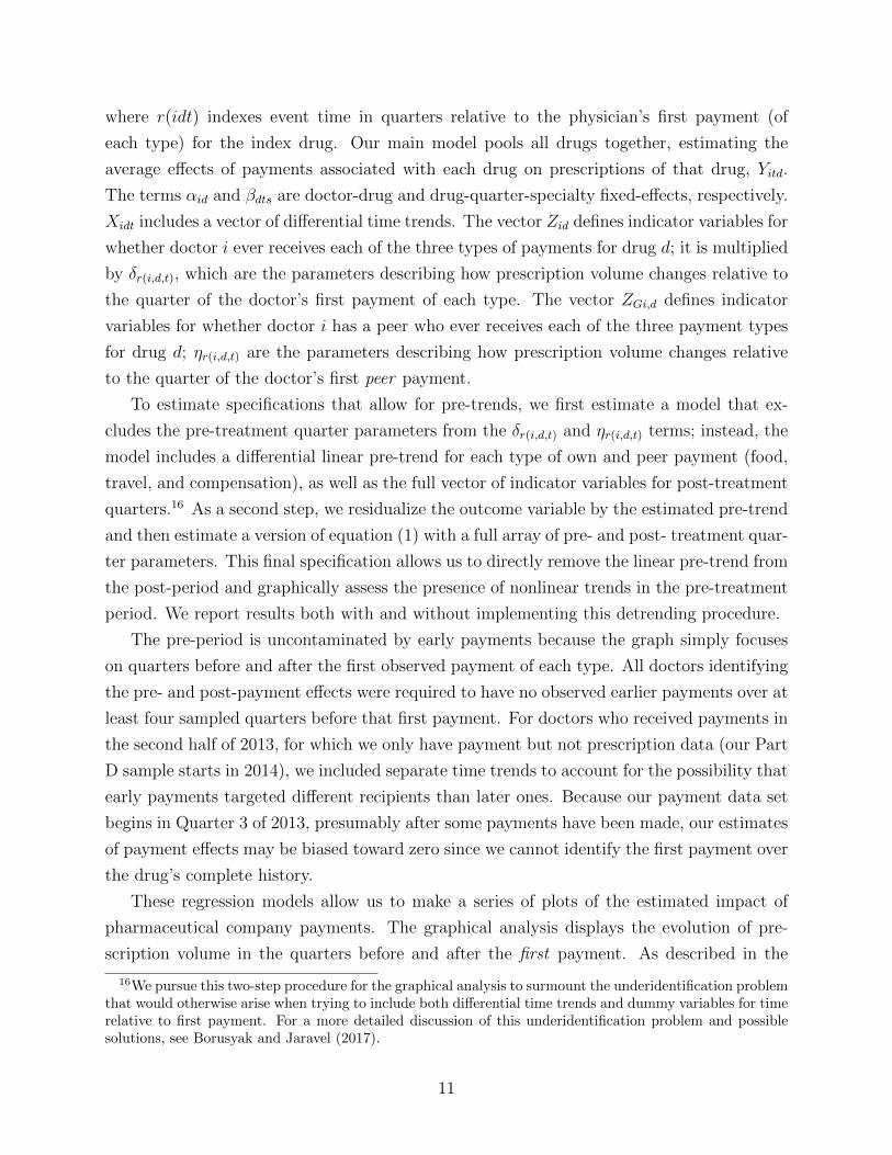
where r(idt) indexes event time in quarters relative to the physician’s first payment (of
each type) for the index drug. Our main model pools all drugs together, estimating the
average effects of payments associated with each drug on prescriptions of that drug, Yitd.
The terms αid and βdts are doctor-drug and drug-quarter-specialty fixed-effects, respectively.
Xidt includes a vector of differential time trends. The vector Zid defines indicator variables for
whether doctor i ever receives each of the three types of payments for drug d; it is multiplied
by δr(i,d,t), which are the parameters describing how prescription volume changes relative to
the quarter of the doctor’s first payment of each type. The vector ZGi,d defines indicator
variables for whether doctor i has a peer who ever receives each of the three payment types
for drug d; ηr(i,d,t) are the parameters describing how prescription volume changes relative
to the quarter of the doctor’s first peer payment.
To estimate specifications that allow for pre-trends, we first estimate a model that ex-
cludes the pre-treatment quarter parameters from the δr(i,d,t) and ηr(i,d,t) terms; instead, the
model includes a differential linear pre-trend for each type of own and peer payment (food,
travel, and compensation), as well as the full vector of indicator variables for post-treatment
quarters.16 As a second step, we residualize the outcome variable by the estimated pre-trend
and then estimate a version of equation (1) with a full array of pre- and post- treatment quar-
ter parameters. This final specification allows us to directly remove the linear pre-trend from
the post-period and graphically assess the presence of nonlinear trends in the pre-treatment
period. We report results both with and without implementing this detrending procedure.
The pre-period is uncontaminated by early payments because the graph simply focuses
on quarters before and after the first observed payment of each type. All doctors identifying
the pre- and post-payment effects were required to have no observed earlier payments over at
least four sampled quarters before that first payment. For doctors who received payments in
the second half of 2013, for which we only have payment but not prescription data (our Part
D sample starts in 2014), we included separate time trends to account for the possibility that
early payments targeted different recipients than later ones. Because our payment data set
begins in Quarter 3 of 2013, presumably after some payments have been made, our estimates
of payment effects may be biased toward zero since we cannot identify the first payment over
the drug’s complete history.
These regression models allow us to make a series of plots of the estimated impact of
pharmaceutical company payments. The graphical analysis displays the evolution of pre-
scription volume in the quarters before and after the first payment. As described in the
16We pursue this two-step procedure for the graphical analysis to surmount the underidentification problemthat would otherwise arise when trying to include both differential time trends and dummy variables for timerelative to first payment. For a more detailed discussion of this underidentification problem and possiblesolutions, see Borusyak and Jaravel (2017).
11
summary statistics reported in Table 1, most paid doctors receive repeated payments of the
same type. As a result, the post-period of these graphs should not be interpreted as the
effect of a single payment, but rather the accumulating effect of all payments received over
those quarters.
Main specification. The event study graphs illustrate a trend break in prescription vol-
ume after the first payment. A key reason for this apparent trend break is that most doctors
in our sample receive repeated payments in the post-period. Thus, for the primary regres-
sion specification reported in our tables, we use the running sum of paid quarters as the key
independent variable to capture the individual impact of each payment. We estimate:
where Pitd denotes a vector of variables that count the number of quarters up to time t with
payments of each type (food, travel, compensation) made to physician i for drug d. PGi,d,t
similarly counts the number of payments (food, travel, compensation) made to doctor d’s
peers (Gi, d, t) up to time t.17 The control variables in (2) parallel those in (1), including the
same set of fixed-effects. We continue to include differential time trends by own and peer
payment type (food, travel, and compensation) for doctors who receive payments in 2013,
before the beginning of our Part D sample. In addition, this specification includes additively
separable trends by own and peer payment type for any doctor who is paid for the first time
during our sample period, which allows for differential pre-trends for doctors paid during
our sample.18
The key parameters of interest are the δ vector, which captures the effect of each ad-
ditional quarter with own pharmaceutical payments of each type, and the η vector, which
captures the effect of the number of peer-quarter pairs that received each type of payment
to date.
17Both the Pidt and PGi,d,t variables are set to zero for doctors who are never (own or peer) paid and fordoctors who receive their first (own or peer) payment of this type in the two quarters before our Part Dsample begins.
18Recall from the discussion in Section 1.2, that we also drop doctor-drug pairs from the sample whenwe do not have at least two pre-payment quarters and two post-payment quarters covered by the Part Dsample. This restriction is imposed for all types of own payment (food, travel, compensation) as well asfor peer compensation payments. We make this restriction so that we have enough in-sample quarters tocontribute to pre/post comparisons within each doctor for our key payment types. This structure ensuresthat all doctors who contribute directly to identification of payment impact (i.e. take nonzero variables ofthe cumulative payment counts) were unpaid for at least four quarters prior to the first payment. We checkthat our results are robust to these sample restrictions by comparing them with an alternative sample thatdrops all doctors who received a payment of any type or who had a compensation-paid peer for the targetdrug during the first three quarters in our sample (see Appendix Table A4).
12
Extensions and robustness checks. We estimate several variants of equation (2). First,
we consider three outcome measures related to physician prescription volume for the target
drug: the number of distinct beneficiaries prescribed, the number of beneficiaries receiving
the target drug as their first anticoagulant prescription, and the fraction of anticoagulant
prescriptions written for the target drug. Second, to explore how the impact of peer payment
varies by the type of relationship, we test augmented specifications that differentiate three
types of physician peer relationships: those defined by shared-patient ties, those defined
by shared group practice affiliation, and those that have both. Third, we test whether
pharmaceutical payments increase adherence to clinical guidelines (see Section 4). Fourth,
we test whether payments affect prescriptions of competing drugs (see Section 6).
Additional models that we use for robustness and heterogeneity analysis test for a differ-
ential impact of the first payment of a given type relative to subsequent payments; estimate
the model separately for each drug; and estimate the model separately for each physician
medical specialty. We also use an alternative regression approach that relies on matching
compensation paid physicians to unpaid physicians who have similar observable character-
istics. The matching approach is discussed in Section 3.4.
2.2 Scaling payment effects by peer prescription volume
As a supplement to the main specifications, we conduct a scaling exercise to explore possible
mechanisms of peer effects. There are two key channels by which having a peer targeted with
a pharmaceutical payment may raise a doctor’s prescribing, holding constant any directly
received payments. First, seeing a colleague prescribe a new drug may provide a positive
signal about the value and applications of the new product, increasing the odds that a doctor
adopts the new drug and prescribes it himself. Second, paid physicians may directly influence
their peers through direct “proselytizing” about the new drug. We apply a two-stage least
squares (2SLS) strategy that attributes peer influence to the indirect mechanism and allows
us to estimate an upper bound on the possible magnitude of indirect influence.
Our 2SLS approach uses detailing payments to a physician’s peers as an instrumental
variable (IV) for peers’ average prescription volume. We then trace the influence of peer
prescriptions on own prescribing. The reduced form of this 2SLS approach is similar to
the preceding analysis, which studies the link between peer payments and the doctor’s own
prescription volume. The IV provides a way to scale this relationship by attributing the
effect to increases in the average prescription volume of the doctor’s peers.
The IV framework continues to exploit the panel data structure to isolate changes in
prescribing patterns that coincide with peer payment shocks.The first- and second-stage
where YGi,d,t is the mean prescription volume of each drug d by i’s peers at t, and PGi,d,t
is a vector of excluded instruments calculating the cumulative sum of the number of peer-
quarter pairs with prior payments of each type (food, travel, compensation) for the target
drug. We continue to control for the doctor’s own payments of each type. Xidt echoes the
trends included in equation (2): differential time trends for each category of own and peer
payment, and differential trends for doctors whose first payment comes before the beginning
of our study period. We estimate the model using two stage least squares.
To interpret this model as the causal effect of peers’ average prescription volume on
the focal doctor requires a strong exogeneity assumption: peer payments are uncorrelated
with unobservable variables affecting the focal doctor’s own prescriptions (E[vidtPGi,d,t] = 0).
Under this assumption, the 2SLS approach will provide an unbiased estimate of peer effects,
eliminating both reflection bias and exclusion bias (Caeyers and Fafchamps 2016).
The exclusion restriction imposes the strong assumption that there is no “direct” effect
of a peer’s payment on a doctor’s own prescription volume except through the channel
of increases in peer prescriptions. For example, if a paid doctor began proselytizing to
his peers about the target drug, and this proselytizing had an independent effect on his
peers’ prescription decisions, then the instrumental variable specification would overstate
the importance of changes in peer prescriptions for doctors’ own prescription decisions.
Based on our conversations with physicians and consultants with expertise in drug de-
tailing, we hypothesize that the indirect peer influence mechanism is more likely, particularly
given the social and institutional distance between most physicians who share patients. This
hypothesis is further bolstered by our finding that estimated peer effects do not exert a
stronger influence among physicians who practice at the same location and therefore pre-
sumably have more opportunities for “proselytizing,” holding fixed the volume of shared
patients between two doctors.
Nevertheless, we proceed cautiously. Because the IV exogeneity assumption could plau-
sibly be violated, we interpret the IV result as an upper bound on the magnitude of the
indirect learning channel. When interpreting this estimate as an upper bound, we are as-
suming that any other channels (such as proselytizing) that lead peer payments to change
the focal doctor’s own prescription patterns would also have the effect of increasing the focal
doctor’s prescription volume.
14
2.3 Discussion of econometric approach
These specifications address several threats to identification of peer effects that arise with
data on groups (Manski 1993) or with cross-sectional, rather than longitudinal, data on
networks (Bramoulle et al. 2009). The problem with group peer relationships (e.g., all
physicians affiliated with a hospital) is that being in the same group is mostly a transitive
relation; therefore, there is little variation in the reference groups of similar agents.19 In con-
trast, physician shared-patient networks are intransitive—even physicians who interact with
each other generally interact with different sets of peers (only a third of connected triplets
are fully connected). Longitudinal data contribute variation in the timing of payments. Our
strategy uses both the across-doctor variation in peer groups and the within-doctor variation
in the timing of payment to identify treatment effects. Through the inclusion of doctor-drug
fixed effects, the framework accounts for the possibility that payments are associated with
unobserved time-invariant physician characteristics. For example, if pharmaceutical transfers
target doctors who were already high-volume prescribers, this would not bias our findings.
Threats to the identification could arise with this approach if payments coincide with
changes in prescription volume for the target drug, which would have occurred even in
the absence of payment. One benefit of focusing on the peers of targeted doctors is that
these peers have not been directly selected by the pharmaceutical company, making it more
plausible that they would otherwise experience parallel trends to other doctors of the same
specialty and eventual payment status. We assess the plausibility of the parallel trends
assumption through graphical analysis of pre-trends prior to the first payment.
3 Results
3.1 Event study graphs of payment impact
We begin by estimating equation (1) to explore the relationship between peer payment
and prescription volume. Figure 1 graphs explore the stability of pre-trends prior to the
first payment. These graphs plot the event-time coefficients from a regression in which
the outcome is quarterly prescription volume, calculated at the physician level. Quarter 0
indicates the first observed quarter in which the physician receives a payment of the indicated
type.
In Figure 1, Panel (A), we show results from a specification that does not account for
differential pre-trends by the doctor’s eventual payment status. These graphs illustrate that
paid doctors are indeed on a trend of increasing use even prior to their first payment; this
19The exception is partially overlapping groups (cf. De Giorgi et al. (2010)).
15
pattern holds for doctors who are targeted with compensation and food payments, as well
as for doctors whose peers receive compensation. Accounting for these pre-trends, we see a
trend break with accelerating growth in prescription volume after the first payment.
Figure 1, Panel (B) displays the same results in a more flexible specification that allows
for differential pre-trends, as described in Section 2.1. The quarters prior to the doctor’s
first payment now show a flat pattern of prescription volume, implying that there is no
acceleration in target drug prescribing before the first payment.
Note that the scale of the y-axis varies across each subplot. Own compensation has the
largest impact on subsequent prescriptions, with prescription volume to 0.34 additional in-
sample patients per quarter within six months of the doctor’s first compensation payment;
this effect amounts to 62 percent of the average quarterly prescription volume of a physician
in our sample.20 Prescriptions also rise after the first food payment by 0.04 additional
patients per quarter, or 7 percent of the average volume, within six months. Finally, after a
peer physician receives a compensation payment, the targeted doctor’s peers increase their
prescription of the new drug by 0.02 additional in-sample patients per quarter, or 3 percent
of the average volume. While these in-sample effect sizes appear modest, recall that in-
sample patients account for only 18 percent of total NOAC prescription volume, and volume
outcomes are reported quarterly (see Section 1.2).
Prescription volume deviates further from the trend as more quarters elapse following the
first payment. This pattern is especially salient following the first food and peer compensa-
tion payments. Recall that many doctors are exposed to repeated shocks of the same type;
the growth in the post-period may reflect the accumulating impact of subsequent payments.
For this reason, we avoid simple pre/post comparisons in our main regression results and
instead model the prescription volume as a function of cumulative payment exposure.
3.2 Baseline regression estimates of payment influence
To unpack the individual impact of each payment, we turn to regression results reported
in Table 3. These results are from direct estimates of equation (2). The key independent
variables in these regressions count the number of quarters to date in which the doctor
received a payment of each type.
Table 3, column 1 reports that doctors increase the quarterly number of prescribed ben-
eficiaries by 0.37 for each additional quarter with a compensation payment, or 65 percent
of the mean quarterly prescription volume in our sample. Smaller transfers have smaller
estimated effects; each quarter with a compensation payment increases a doctor’s own pre-
20Recall that the average quarterly prescription volume across all doctors in our sample is 0.55 beneficiaries.
16
scribing by 0.06 additional prescribed beneficiaries per quarter, or 10 percent of the average
volume. Having a peer doctor receive a compensation payment leads to a modest increase
in own prescription volume of 0.02 additional beneficiaries per month, or 3 percent of the
average volume. Recall that while every specification also accounts for the impact of own and
peer travel payments, we are not reporting these coefficients in our main tables because this
payment type is less frequent and we are generally not powered to detect effects; complete
results are reported in Appendix Table B1.
Comparing the estimated increases in prescription volume to the pooled average pre-
scription volume in our sample masks heterogeneity in average prescription volumes between
recipients of different payment types. Comparing the same estimates to the 2014–2016 av-
erage prescription volume of each group of recipients, we see the increase in prescription
volume due to compensation payments is 6 percent of the 5.94 prescribed beneficiaries per
quarter among large payment recipients, 5 percent of the average 1.11 prescribed benefi-
ciaries per quarter among food recipients, and 1.8 percent of the average 1.12 prescribed
beneficiaries per quarter among peers of large payment recipients. When interpreting these
group averages, note that they are calculated over the entire sample period and partly reflect
prescription responses to payments.
One possible mechanism behind the peer effects we estimate are prescription refills, which
may happen when a primary care physician orders a refill of a prescription that was initi-
ated by a compensated cardiologist. As the primary care physician becomes more familiar
with the new drug, she may also choose to initiate new prescriptions with the drug. To
estimate the effects of payments on prescriptions to new patients, we exclude prescription
refills by restricting our prescription volume outcome to only include patients without any
prior prescription for anticoagulants in the previous year (Table 3, column 3). Between 8 to
10 percent of the effect of payment on total prescription volume is driven by prescriptions
written for patients with no prior anticoagulant use. This result includes peers of payment
recipients, suggesting the spillover effects of payments on peers also spur prescriptions of the
target drug to new patients.
Next, we turn to a third outcome measure: the fraction of anticoagulant prescriptions
that were written for the target drug. This outcome measure will allow us to test whether
the increases in prescription volume measured in the prior specifications were driven by an
increase in the total volume of anticoagulant prescriptions, or alternatively, whether within
the set of anticoagulant prescriptions, doctors are shifting patients toward the target drug.
This outcome is only defined for the 68 percent of doctor-drug-quarters from our full sample
that have nonzero anticoagulant prescriptions during the quarter.
Results from this specification are reported in Table 3, columns 5 and 6. Own food
17
payments and peer compensation payments are associated with a significant increase in
market share of the target drug. Estimates for the effects of own compensation payments on
drug market share are not statistically significant, but point estimates are consistent with
an increase in market share following direct payments.
A back-of-the-envelope calculation suggests that the estimated returns to payments for
the pharmaceutical companies are positive. Assume an average revenue of $800 per pre-
scribed beneficiary per quarter, roughly the average in our sample (see Appendix Figure A2),
and consider that spending on food and education payments is approximately $30 per trans-
action. Food payments are estimated to yield 0.06 new prescriptions each quarter in our
40 percent Medicare sample, which corresponds to an additional quarterly revenue of $260
when both Medicare and non-Medicare patients are considered.21 In contrast, compensation
payments of $3,000 per quarter would appear less profitable if only their direct effect is ac-
counted for, because the 0.37 new beneficiaries it is estimated to add in our sample reflect
only $1,600 of additional revenue. However, including the additional 0.02 patients such pay-
ments yield in our sample for each of the 60 (on average) peers of the direct recipient, means
that their overall return is much greater, as spillovers alone generate an additional $4,800
per payment. These rough estimates suggest that accounting for spillover effects is essential
for evaluating the return on pharmaceutical payments, particularly for large payments. We
further discuss the aggregate impact of payments in Section 5.
Recall that our baseline definition of peer affiliation is based on patient-sharing patterns.
In the regression specification reported in Table 4, we also consider peer relationships based
on group practice affiliation. We distinguish three types of peer relationships: doctors who
share patients, doctors who share both patients and a group practice affiliation, and doctors
who only share a group practice affiliation. The results suggest that doctors who share
patients with a compensation-paid peer will increase their prescribing volume by 0.02 per
quarter in our sample, while doctors who not only share patients but also a group practice
affiliation with a compensation-paid peer will increase their prescribing volume by 0.014 in
sample patients.22 This difference between the two peer types is not statistically significant.
Doctors who only share a group practice affiliation (but do not have shared patients) with
the compensation-paid peer increase their prescription volume of the target drug by 0.014
patients per quarter. Taken together, these results suggest that compensation payments
increase drug prescription volume of both peer types; our results are not driven solely by
21The estimated overall value of added prescriptions comes from scaling the regression coefficients fromTable 3 upward by a factor of 5.4, which accounts for non-sampled Medicare beneficiaries, as well as non-Medicare patients, as discussed in Section 1. For the food example, this is 0.0589 · 5.4 = 0.324
22As reported in Table 4, column 2, 0.014 is the sum of the ”Shared patient” and the ”Group practice andshared patient” coefficients.
18
doctors who share a group practice.
3.3 Assessing the scale of peer effects in prescribing
In this section, we focus on the first learning mechanism and estimate the impact of an
increase in peers’ prescription volume for a new drug on a doctor’s own prescription volume.
As discussed in Section 2, we use the number of peer compensation, peer travel and peer
food payments to date as instrumental variables for the average prescription volume across
each physician’s direct peers. We then trace out the influence of peer prescriptions on own
prescribing.
If we assume that paid doctors do not directly promote the drugs to their peers (the
“proselytizing” mechanism), then these instrumental variable estimates of peer effects may
generalize to settings in which peer prescription decisions are not driven by pharmaceutical
payments. As we cannot rule out proselytizing behavior, we will interpret our instrumental
variable estimates as an upper bound on the magnitude of peer effects we would expect when
prescription patterns change for reasons other than a pharmaceutical payment.
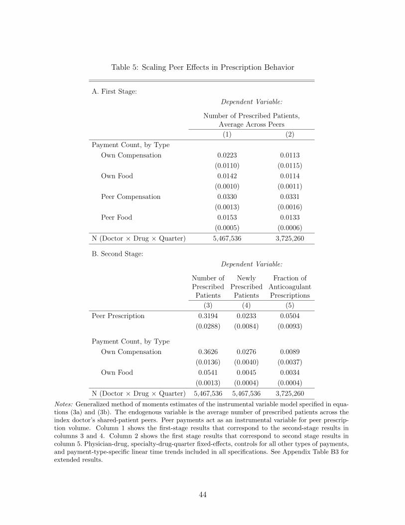
First-stage estimates suggest that an additional compensation payment to a doctor’s peer
raises the quarterly prescription volume averaged across all of the doctor’s peers by 0.033
beneficiaries per quarter (statistically significant at the 1 percent level; Table 5). This effect
is much smaller than the estimated impact of a large payment on the targeted doctor himself,
reflecting the fact that we are averaging prescriptions across all doctors’ peers, only one of
whom was hit with the payment shock. This averaged impact reflects a combination of the
direct impact of a large payment on the targeted physician as well as any ripple effects due
to peer linkages between the paid physicians’ peers and other peers.
Second-stage regression estimates show that if the average prescription volume across the
focal doctor’s peers increases by one beneficiary per quarter on average, the focal doctor’s
own prescription volume will increase by 0.32 prescriptions per quarter. Should this finding
be driven by indirect observation of peer prescription choice (rather than proselytizing), it
suggests that the prescription increases may ripple (with decay) beyond first-degree peer
connections.
3.4 Robustness and treatment effect heterogeneity
In this section we explore alternative specifications and probe whether the estimated effects
of physician payments are heterogeneous across the sequence of payments or the type of
doctor targeted.
19
First, we test an alternative regression approach that relies on matching compensation-
paid physicians to unpaid physicians who have similar observable characteristics. We con-
struct the matched sample of paid and unpaid physicians as follows. First, we sample
all physicians who received compensation payments at any point during 2014–2016. We
henceforth refer to these physicians as targets. Second, we match each target with similar
physicians who did not receive compensation payments, based on the following criteria.
We match exactly on specialty, the target drug, and location (HRR). We match coarsely
(by quartiles) on experience, number of shared-patient peers, and number of group practice
peers. We also drop a small number of matches who share a group practice with the target, so
all our matches are from the same area as the target but not from the same practice. We then
sample all shared-patient peers of targets and their matches. We exclude peers of targets
or matches who have an additional peer (beyond the target) who received compensation
payments. Therefore, the resulting sample has two disjoint sets of physicians who are peers
of either a paid physician or a matched unpaid one, and who have no other compensation-
paid peers.
Descriptive statistics for the matched sample are shown in Table A3. Results from the
matching estimation are reported in Table 6. Columns 1, 3, and 5 replicate the baseline
specification included in Table 3 on the matched sample. Columns 2, 4, and 6 show similar
results with an alternative specification that excludes differential time trends for doctors paid
during our Medicare Part D sample period. Our matched sample yields very similar results
to our baseline estimates. In the matched sample, we find that the focal doctor increases
his prescription volume of the target drug by 0.025 patients per quarter for each additional
compensation payment targeted at the focal doctor’s peers (see Table A3, column 1); for
comparison, the baseline estimate was 0.018.
In Appendix Table A4, we report additional robustness checks, varying the specification
and the estimating sample. Column 1 replicates our baseline estimates (as reported in
Table 3) with doctor-drug fixed effects. Column 2 substitutes the fixed effects with random
effects at the doctor-drug level, which will yield unbiased estimates of payment impact only
if payments are conditionally uncorrelated with doctors’ baseline propensity to prescribe
the new drug. We find very similar results from the random effects specification; as before,
each compensation payment paid to a focal doctor’s peer is estimated to increase the focal
doctor’s prescribing by 0.02 in-sample beneficiaries per quarter. We use this random effects
specification as the basis for our counterfactual analysis reported in Section 5. Finally, in
column 3, we estimate our baseline fixed effects model on a restricted sample of doctors;
this specification drops doctors directly receiving a payment of any type prior to 2014Q3
as well as doctors who have a compensation-paid peer for the target drug prior to 2014Q3.
20
Estimated peer effects of compensation payments remain similar in this sample; having a
compensated peer increases prescribing by 0.015 in-sample beneficiaries per quarter.
In Appendix Table A5, we test whether the first observed payment has a differential
impact relative to subsequent payments.23 The coefficients on the “first payment” variables
should be interpreted as the difference in the effect of the first payment compared to the
effect of subsequent payments; to calculate the total impact of the first payment, the first and
count coefficients should be added. Point estimates suggest that a doctor’s first compensation
payment and first food payment have slightly smaller estimated effects than subsequent
payments. The first time a doctor’s peer receives a compensation payment it has a nearly
zero estimated impact on the doctor’s prescription volume, although this estimate is noisy
and not statistically distinguishable from the impact of subsequent payments.
Similar results for the effects on payments on prescriptions are obtained when we estimate
the effects separately by medical specialty, or by drug, as reported in Appendix Table A6.
The first row shows our baseline specification. The second and third rows show results
separately by specialty. Peer payments both lead to a larger increase in prescription volume
for cardiologists. This pattern is consistent with the fact that cardiologists write more
prescriptions for anticoagulants in general, and therefore have more scope to increase their
use of target drugs. The remaining rows show estimates of the influence of payments on
prescriptions, separately for each drug. Point estimates suggest that own and peer payments
increase prescription volume for each of the three NOACs under study. The effect of peer
compensation payments on the quarterly number of prescribed patients is similar for Xarelto
(0.025) and Eliquis (0.023), and smaller for Pradaxa (0.009), although these comparisons are
imprecise.
4 Welfare Implications
A highly contested question is how pharmaceutical detailing payments impact patient wel-
fare. On the one hand, payments may lead physicians to over-prescribe high cost drugs.
On the other hand, pharmaceutical companies argue that detailing improves welfare by ed-
ucating physicians about new drugs and providing up-to-date information to support better
practice.
To investigate this question, we analyzed whether pharmaceutical payments lead to in-
creased adherence to evidence-based clinical guidelines on anticoagulant prescriptions. Be-
23Recall that because we observe only a censored history of pharmaceutical payments, we cannot defini-tively identify each doctor’s first payment. Instead we tag the earliest payment observed in our sample periodas the “first”, and we require that doctors identifying our main regression coefficients had no payments fora minimum of four preceding quarters.
21
cause guidelines are not available to cover all patient indications for anticoagulant drugs, we
narrow our focus to patients with atrial fibrillation, which is a common reason for prescribing
anticoagulants. There are two popular risk scores to assess the risks and benefits of antico-
agulation for patients with atrial fibrillation: the HAS-BLED and CHADS2 scores (Pisters
et al. 2010; Lip et al. 2011; Gage et al. 2001, 2004).The HAS-BLED score estimates risk of
bleeding for patients on anticoagulation drugs, which is the major safety concern that should
be weighed against the stroke reduction benefits of the drug. The CHADS2 score estimates
the gains from anticoagulation.24 Note that current guidelines provide little guidance on
selecting among the various anticoagulant drugs; rather, they focus on determining whether
the patient is appropriate for anticoagulation drugs at all.25
We use the CMS Chronic Condition Warehouse data file to identify patients with diag-
nosed atrial fibrillation. As before, we count the number of unique beneficiaries prescribed
anticoagulants by each doctor in each quarter, but for this analysis we restrict the prescrip-
tion count to include only patients with diagnosed atrial fibrillation. Within this sample, we
construct an estimate of the HAS-BLED risk score and CHADS2 score for each prescribed
patient.
We observe four of the nine clinical characteristics included in the HAS-BLED score to
construct our estimate: patient age > 65, hypertension history, renal disease, and stroke
history.26 The guideline is scored simply: one point per risk factor. Patients scoring zero to
one are considered low risk; two points correspond to moderate risk; three or more points
correspond to high risk.27
Because we do not observe all the factors that underlie this guideline, we interpret our
results as follows. Patients who have three or more risk factors are designated high risk;
24For a quick reference guide to clinical scoring for atrial fibrillation, see MDCalc https:
//www.mdcalc.com/has-bled-score-major-bleeding-risk and https://www.mdcalc.com/
26Even among our observed patient characteristics, our definitions do not exactly align with the definitionsused in the guideline. For example, hypertension is only considered if it is uncontrolled and the patient has> 60 mmHg systolic pressure. A similarly precise definitions is used for renal disease. Patient characteristicsincluded in the full HAS-BLED score but not observable in our data include: labile INR (a lab blood testvalue), prior major bleeding or predisposition to bleeding, liver disease, medication use predisposing tobleeding (including aspirin and NSAIDS that are not prescription drugs), and alcohol use (at least eightdrinks per week).
27Note that the guidelines themselves do not provide sharp recommendations on whether or not to prescribeanticoagulation drugs. For example, the HAS-BLED score recommendations provided on MDCalc.comare worded as “anticoagulation should be considered” [strongest recommendation], “anticoagulation can beconsidered” [moderate], or “alternatives to anticoagulation should be considered” [weakest].
where, as before, where i indexes doctors, t indexes time, s indexes their medical specialty,
and d indexes the target drug. The dependent variable of the first equation, Yi,t,d, denotes
prescriptions of the target drug. The dependent variable in the second equation,∑
d′ 6=d Yi,t,d′ ,
denotes prescriptions of all other coagulants, except for d. The rest of the terms are defined
exactly as in equation (2). Here, we are interested in comparing the elasticity of prescriptions
of the target-drug and the cross-drug elasticity with respect to own payments (δ and δ) and
peer payments (η and η).
We test the null hypothesis that the sum of the additional number of target and competi-
tor prescriptions that is due to payment of each type is zero, using a χ2 test. If this sum is
zero, it implies that on average, the increase in prescription volumes due to payments mainly
reflects business stealing. We perform this test for each of the six payment types separately.
Namely, we test whether δj + δj = 0, where j is each one of food, travel, and compensation.
We also perform this test for own payments of all types combined (δ + δ = ~0), and for peer
payments of all types combined (η + η = ~0).
The results of this analysis are summarized in Table 8. The first column shows the
SUR estimates of the effects of different types of payments on prescriptions of the target
drug. The coefficient estimates are identical to our OLS estimates of equation (2), shown
in Table 3, except with updated standard errors that account for the cross-equation error
structure. Column 2 shows the effects of payments associated with each target drug on
27
prescriptions of the competitors. We estimate that receiving compensation or consulting
fees or having a peer receive such a payment is not associated with a significant change in
prescriptions of competitor drugs. Namely, the increase in prescriptions due to compensation
payments is concentrated mostly in the target drug, and reflects neither business stealing
nor an expansion of anticoagulant use beyond the target drug. In contrast, we estimate
that physicians who receive food payments prescribe both the target and the competitor
drugs more, suggesting that detailing visits spillover positively to competitors and induce
a market expansion.29 Payments made to peers have small negative effects on competitor
drug prescriptions, but these effects are not statistically insignificant. Columns 3 shows the
results of the χ2 tests, rejecting the null that payments increase prescriptions merely through
business stealing (p < 0.001 for own and p = 0.029 for peer payments).
7 Conclusion
Pharmaceutical companies pay physicians large sums of money, in the form of payments for
services or in-kind transfers. Survey evidence suggests these payments are widespread, with
94 percent of US doctors reporting some form relationship with pharmaceutical companies
and 25 percent receiving a payment from a pharmaceutical company for compensation or
consulting services within the past year (Campbell et al. 2007). Using rich administrative
data on prescriptions, payments, and physician networks, and exploiting variation in both the
timing and targeting of payments, this study has shown that pharmaceutical payments lead
to a significant and persistent increase in the prescription of new anticoagulant drugs. Larger
payments for consulting and compensation for services have a greater effect on prescriptions
than small payments of food and beverages. We find no evidence that payments improved
adherence to clinical guidelines.
Furthermore, large payments from pharmaceutical firms, which target a small group of
specialized and highly connected physicians, have substantial spillover effects—they lead not
only to increased prescriptions by recipients, but also by the recipients’ peers. The mag-
nitude of these spillovers is substantial. The indirect influence through spillovers of each
large payment is several times greater than its direct effect. Overall, spillover effects of phar-
maceutical payments account for about a quarter of their estimated impact on prescription
volumes.
Our results suggest that learning from peers is an important channel through which
29Note that the counterfactual estimates of the overall effects of payments on prescription volumes, pre-sented in Section 5, only regard the influence of payments on the target drugs. Therefore, the positive effectof food payments on the prescription of competitor products suggests that the contribution of payments toprescription volumes of all anticoagulants—including competitors—is even greater.
28
pharmaceutical payments impact clinical practice. This finding corroborates accounts of
marketing strategies that leverage influential individuals for wider impact. More broadly,
these results suggest that peer influence may be an important channel for adoption of new
technologies in medicine.
This project leaves several open questions. In future work, it would be instructive to
extend this framework to study spillover effects of marketing in the diffusion of other tech-
nologies. Additionally, it would be interesting to explore whether similar peer effects arise
when practice patterns change for reasons other than pharmaceutical payments. Our find-
ings suggest that policy interventions to increase prescribing of recommended drugs may
achieve a broader reach by targeting highly connected physicians, but rigorous evaluation
should test whether peer spillovers extend to other settings.
References
Agha, Leila and David Molitor, “The Local Influence of Pioneer Investigators on Tech-nology Adoption: Evidence from New Cancer Drugs,” The Review of Economics andStatistics, 2018, 100 (1), 29–44.
Banerjee, Abhijit, Arun G. Chandrasekhar, Esther Duflo, and Matthew O Jack-son, “The diffusion of microfinance,” Science, 2013, 341 (6144), 1236498.
Barnett, Michael L., Bruce E. Landon, A. James O’Malley, Nancy L. Keating,and Nicholas A. Christakis, “Mapping physician networks with self-reported and ad-ministrative data,” Health Services Research, 2011, 46 (5), 1592–1609.
Berndt, Ernst R., Linda Bui, David R. Reiley, and Glen L. Urban, “Information,marketing, and pricing in the US antiulcer drug market,” The American Economic Review,1995, 85 (2), 100–105.
, , David Reiley, and Glen Urban, “The Roles of Marketing, Product Quality andPrice Competition in the Growth and Composition of the U.S. Anti-Ulcer Drug Industry,”Working Paper 4904, National Bureau of Economic Research October 1994.
Borusyak, Kirill and Xavier Jaravel, “Revisiting event study designs,” Available atSSRN 2826228, 2017.
Bramoulle, Yann, Habiba Djebbari, and Bernard Fortin, “Identification of peereffects through social networks,” Journal of Econometrics, 2009, 150 (1), 41–55.
Caeyers, Bet and Marcel Fafchamps, “Exclusion Bias in the Estimation of Peer Effects,”Working Paper 22565, National Bureau of Economic Research August 2016.
Campbell, Eric G., Russell L. Gruen, James Mountford, Lawrence G. Miller,Paul D. Cleary, and David Blumenthal, “A national survey of physician–industryrelationships,” New England Journal of Medicine, 2007, 356 (17), 1742–1750.
29
Campbell, John J., Understanding Pharma: The Professional’s Guide to how Pharma-ceutical and Biotech Companies Really Work, Pharmaceutical Institute, 2008.
Carey, Colleen Marie, Ethan MJ Lieber, and Sarah Miller, “Drug Firms’ Paymentsand Physicians’ Prescribing Behavior in Medicare Part D,” Available at SSRN 2663681,2015.
Chan, David C., “Influence and Information in Team Decisions: Evidence from MedicalResidency,” Working Paper, 2018.
CMS, “Physician Shared Patient Patterns,” 2013. data retrieved from http://downloads.
Coleman, James, Elihu Katz, and Herbert Menzel, “The Diffusion of an InnovationAmong Physicians,” Sociometry, 1957, 20 (4), 253–270.
Cutler, David, Jonathan S. Skinner, Ariel D. Stern, and David Wennberg, “Physi-cian Beliefs and Patient Preferences: A New Look at Regional Variation in Health CareSpending,” American Economic Journal: Economic Policy, 2019, 11 (1), 192–221.
David, Guy, Sara Markowitz, and Seth Richards-Shubik, “The effects of pharma-ceutical marketing and promotion on adverse drug events and regulation,” American Eco-nomic Journal: Economic Policy, 2010, 2 (4), 1–25.
DeJong, Colette, Thomas Aguilar, Chien-Wen Tseng, Grace A. Lin, W. JohnBoscardin, and R. Adams Dudley, “Pharmaceutical industry–sponsored meals andphysician prescribing patterns for Medicare beneficiaries,” JAMA Internal Medicine, 2016,176 (8), 1114–1122.
Donohue, Julie M., Hasan Guclu, Walid F. Gellad, Chung-Chou H. Chang,Haiden A. Huskamp, Niteesh K. Choudhry, Ruoxin Zhang, Wei-Hsuan Lo-Ciganic, Stefanie P. Junker, Timothy Anderson, and Seth Richars-Shubik, “In-fluence of peer networks on physician adoption of new drugs,” PLOS One, 2018, 13 (10),e0204826.
, Nancy E. Morden, Walid F. Gellad, Julie P. Bynum, Weiping Zhou, Joseph T.Hanlon, and Jonathan Skinner, “Sources of Regional Variation in Medicare Part DDrug Spending,” New England Journal of Medicine, 2012, 366 (6), 530–538. PMID:22316446.
Gage, Brian F., Amy D. Waterman, William Shannon, Michael Boechler,Michael W. Rich, and Martha J. Radford, “Validation of clinical classificationschemes for predicting stroke: Results from the National Registry of Atrial Fibrillation,”JAMA, 2001, 285 (22), 2864–2870.
, Carl van Walraven, Lesly Pearce, Robert G. Hart, Peter J. Koudstaal, B.S.P.Boode, and Palle Petersen, “Selecting patients with atrial fibrillation for anticoagu-lation: Stroke risk stratification in patients taking aspirin,” Circulation, 2004, 110 (16),2287–2292.
Galeotti, Andrea, Benjamin Golub, and Sanjeev Goyal, “Targeting interventions innetworks,” arXiv preprint arXiv:1710.06026, 2017.
Giorgi, Giacomo De, Michele Pellizzari, and Silvia Redaelli, “Identification of so-cial interactions through partially overlapping peer groups,” American Economic Journal:Applied Economics, 2010, 2 (2), 241–275.
Golub, Ben and Evan Sadler, “Learning in Social Networks,” in Yann Bramoulle, AndreaGaleotti, and Brian Rogers, eds., The Oxford Handbook of the Economics of Networks,Oxford University Press, 2016.
Grennan, Matthew, Kyle Myers, Ashley Swanson, and Aaron Chatterji,“Physician-Industry Interactions: Persuasion and Welfare,” NBER Working Paper No.24864, 2018.
Hoadley, John F, Juliette Cubanski, and Patricia Neuman, “Medicare’s Part D drugbenefit at 10 years: firmly established but still evolving,” Health Affairs, 2015, 34 (10),1682–1687.
Iyengar, Raghuram, Christophe Van den Bulte, and Thomas W. Valente, “Opinionleadership and social contagion in new product diffusion,” Marketing Science, 2011, 30 (2),195–212.
Larkin, Ian, Desmond Ang, Jonathan Steinhart, Matthew Chao, Mark Pat-terson, Sunita Sah, Tina Wu, Michael Schoenbaum, David Hutchins, TroyenBrennan, and George Loewenstein, “Association between academic medical centerpharmaceutical detailing policies and physician prescribing,” JAMA, 2017, 317 (17), 1785–1795.
Lip, Gregory Y.H., Lars Frison, Jonathan L. Halperin, and Deirdre A. Lane,“Comparative validation of a novel risk score for predicting bleeding risk in anticoagulatedpatients with atrial fibrillation: the HAS-BLED (Hypertension, Abnormal Renal/LiverFunction, Stroke, Bleeding History or Predisposition, Labile INR, Elderly, Drugs/AlcoholConcomitantly) score,” Journal of the American College of Cardiology, 2011, 57 (2), 173–180.
MacLeod, Bentley W. and Janet Currie, “Small Area Variations and Physician Deci-sion Making: The Case of Depression,” Working Paper, 2018.
Manski, Charles F., “Identification of endogenous social effects: The reflection problem,”The Review of Economic Studies, 1993, 60 (3), 531–542.
31
Mekaj, Ymer H., Agon Y. Mekaj, Shkelzen B. Duci, and Ermira I Miftari,“New oral anticoagulants: Their advantages and disadvantages compared with vitaminK antagonists in the prevention and treatment of patients with thromboembolic events,”Therapeutics and Clinical Risk Management, 2015, 11, 967.
Moen, Erika L., Andrea M. Austin, Julie P. Bynum, Jonathan S. Skinner, andA. James O’Malley, “An analysis of patient-sharing physician networks and implantablecardioverter defibrillator therapy,” Health Services and Outcomes Research Methodology,2016, 16 (3), 132–153.
Navathe, Amol and Guy David, “The formation of peer reputation among physiciansand its effect on technology adoption,” Journal of Human Capital, 2009, 3 (4), 289–322.
Oster, Emily and Rebecca Thornton, “Determinants of technology adoption: Peereffects in menstrual cup take-up,” Journal of the European Economic Association, 2012,10 (6), 1263–1293.
Pisters, Ron, Deirdre A. Lane, Robby Nieuwlaat, Cees B. De Vos, Harry J.G.M.Crijns, and Gregory Y.H. Lip, “A novel user-friendly score (HAS-BLED) to assess1-year risk of major bleeding in patients with atrial fibrillation: The Euro Heart Survey,”Chest, 2010, 138 (5), 1093–1100.
Sacarny, Adam, Andrew R. Olenski, and Michael L. Barnett, “Association of Que-tiapine Overuse Letters With Prescribing by Physician Peers of Targeted Recipients: ASecondary Analysis of a Randomized Clinical Trial,” JAMA Psychiatry, 2019.
Schwartz, Lisa M. and Steven Woloshin, “Medical Marketing in the United States,1997-2016,” JAMA, 01 2019, 321 (1), 80–96.
Shapiro, Bradley T., “Informational shocks, off-label prescribing, and the effects of physi-cian detailing,” Management Science, 2018, 64 (12), 5925–5945.
, “Positive spillovers and free riding in advertising of prescription pharmaceuticals: Thecase of antidepressants,” Journal of Political Economy, 2018, 126 (1), 381–437.
Silver, David, “Haste or Waste? Peer Pressure and Productivity in the Emergency De-partment,” Working Paper, July 2019. https://www.dropbox.com/s/ril7ugyvenb0ogk/jmp.pdf?dl=0.
Sinkinson, Michael and Amanda Starc, “Ask your doctor? Direct-to-consumer adver-tising of pharmaceuticals,” The Review of Economic Studies, 2018, 86 (2), 836–881.
Skinner, Jonathan and Douglas Staiger, “Technology diffusion and productivity growthin health care,” Review of Economics and Statistics, 2015, 97 (5), 951–964.
Zeltzer, Dan, “Gender homophily in Referral Networks: Consequences for the MedicarePhysician Earnings Gap,” Americal Economic Journal: Applied Economics, forthcoming.
Figure 1: Event Study: The Impact of Payments on Prescription Volume
(A) Before Detrending
●●●
●●●
●● ●
● ●● ●
●●
●●
●●
●
●
●
●●
●●
●●
●●
●●
●●
●● ●
●
●
Own Compensation Own Food Peer Compensation
−6 −3 0 3 6 −6 −3 0 3 6 −6 −3 0 3 6
0.0
0.1
0.0
0.1
−1.0
−0.5
0.0
0.5
1.0
1.5
Quarter relative to first payment
Coe
ffici
ent e
stim
ates
(pr
escr
ibed
pat
ient
s)
(B) After Detrending
●●●●●●
●● ●
●●
●●
●●●●
●●
●
●
●
● ●
●●
●●●●
●
● ● ●●
●
●
●
●
Own Compensation Own Food Peer Compensation
−6 −3 0 3 6 −6 −3 0 3 6 −6 −3 0 3 6−0.05
0.00
0.05
0.10
−0.025
0.000
0.025
0.050
0.075
−0.4
0.0
0.4
0.8
1.2
Quarter relative to first payment
Coe
ffici
ent e
stim
ates
(pr
escr
ibed
pat
ient
s)
Notes: Figure shows event study coefficients estimated from equation (1), showing the response of physiciansto own and peer payments of different types. The facets show coefficients for different payment types—ownfood, own compensation, and peer compensation—that were all jointly estimated using 5,467,536 doctor-drug-quarter observations. Panel (A) reports coefficients from a single regression that excludes a differentialpre-trend for paid physicians; the dashed line fitted to the pre-trend for illustration. Panel (B) reportscoefficients from a single regression after detrending, using the two-step procedure described in Section 2.All regressions also include variables for peer food, own travel, and peer travel, alongside fixed effects fordoctor-drug and drug-specialty-quarter. Quarter 0 indicates the quarter of the first payment of each type.Shaded areas show 95 percent confidence intervals. Note that facet vertical axes have different scales.
33
Figure 2: NOAC Prescription Volume over Time
●
●
●
●
●
●
●
●
●
●
●
●
0.0
0.3
0.6
0.9
2014 2015 2016
Ben
efic
iarie
s P
er P
hysi
cian
Drug● ELIQUIS
XARELTOPRADAXA
Notes: For the three NOAC drugs we study, figure shows the average number of prescribed beneficiariesper quarter per physician in our sample. Averages are over all physician-quarters in our sample,including those with zero prescriptions. The FDA first approved Pradaxa in 2010, Xarelto in 2011, andEliquis in 2012. Data are from 40 percent of Medicare Part D claims.
34
Figure 3: Average Number of Payments per Physician, by Type of Payment and MedicalSpecialty
●
●
●
●
●
●
●
●
●
●
●
●
●
●
●
●
●
●
●
●
●
●
●
●
●
●
●
●
● ●●
●●
●●
●●
●●
●●
●
● ● ● ● ● ● ● ● ● ● ● ● ● ●
Cardiac Specialist Primary Care
Food
Com
pensation
2014 2015 2016 2014 2015 2016
0
1
2
3
4
0.00
0.05
0.10
0.15
Ave
rage
Num
ber
of P
aym
ents
Rec
eive
d
● ELIQUIS XARELTO PRADAXA
Notes: Figure shows average cumulative number of payments per physician in 2014–2016 associatedwith each of the three NOACs in our sample. Each column of facets shows data for a different medicalspecialty: cardiac specialties (left) and primary care (right). Each row of facets shows payments of adifferent type: Food category includes education, food, and beverage transfers; Compensation includescompensation for services and consulting fees. Section 1 describes the specialty and payment categorydefinitions.
35
Figure 4: Average Number of Payments by Recipient Number of Peers
Compensation
Cardiac Specialist
Compensation
Primary Care
Food
Cardiac Specialist
Food
Primary Care
1 2 3 4 5 6 7 8 9 10 1 2 3 4 5 6 7 8 9 10
1 2 3 4 5 6 7 8 9 10 1 2 3 4 5 6 7 8 9 10
0.0
0.5
1.0
1.5
0.000
0.005
0.010
0.015
0.020
0.025
0
1
2
3
4
0.0
0.1
0.2
Number of Peers (Decile, within HRR and Specialty)
Ave
rage
Num
ber
of P
aym
ents
Notes: For each specialty and type of payment, figure shows the average number of payments madeto each physician (y-axis), by deciles of the recipient’s number of peers (x-axis). Deciles are calculatedseparately for each HRR and specialty. Error bars show 95 percent confidence interval for the mean.Note that facet vertical axes have different scales. Each row of facets shows payments of a different type:Food category includes education, food, and beverage transfers; Compensation includes compensationfor services and consulting fees. Each column shows data for a different medical specialty: cardiacspecialties (left) and primary care (righy). For specialty definitions see Section 1.
36
Figure 5: Actual and Counterfactual US Prescription Volumes
●●●
●●
●
●●
●
●●
●
●●
●
●●
●
●
●
●
●
●
●
●
●
●
●
●
●
●
●
●
●
●
●
0
250
500
750
2014 2015 2016
Qua
rter
ly P
resc
riptio
n V
olum
e(U
SD
mill
ions
)
Drug● ELIQUIS
XARELTOPRADAXA
Scenario
Actualwith Payments
Counterfactualw/o Peer Pay
Counterfactualw/o Any Pay
Notes: Figure shows estimated actual and counterfactual total US prescription volume per quarter.Each color represents one drug in our sample. For each drug, the solid line is the actual US quarterlyprescription volume. The dashed line labeled “Counterfactual w/o Peer Pay” is the counterfactualvolume obtained by shutting off any effects of payments to peers of the directly paid physicians. Thedotted line labeled “Counterfactual w/o Any Pay” is the counterfactual volume obtained in the absenceof any pharmaceutical payments. Dollar estimates were obtained by summing the estimated numberof prescribed beneficiaries over all physicians in our sample and multiplying the sum by the averagequarterly prescription cost per patient in our sample (average costs are shown in Figure A2). Allestimates are scaled by a factor of 5.4 to reflect the total US market size, including non-Medicarepatients; the scaling exercise implicitly assumes that the price per prescription is the same for MedicarePart D patients and other patients prescribed the drug. This scaling factor is discussed in Section 1.Estimates of the average number of beneficiaries per doctor before scaling are shown in AppendixFigure A4.
37
Figure 6: Pharmaceutical Payment Impact on Prescription Volumes
(A) Average Payment Impact on the Quarterly Number of Prescribed Benefi-ciaries
Food
Compensation
0.0 0.4 0.8 1.2 1.6
Direct Payment Impact Payment Impact on Peers
(B) Total Number of Payments (2014–2016)
Food
Compensation
0 500,000 1,000,000 1,500,000
(C) Aggregate Payment Impact on Annual Prescription Volume (USD millions)
Food
Compensation
0 250 500 750 1000
Total Direct Impact Total Impact on Peers
Notes: Figure shows estimates of direct and peer effects of pharmaceutical payments on prescription
volume, by type of payment: Compensation are payments for services and consulting fees; Food are
payments for or in-kind transfers of food, beverages, and educational items. Panel (A) shows the
estimated effect of receiving payments of each type during a quarter on the quarterly number of unique
beneficiaries prescribed the target drug by the direct recipient (light shade) and by all of the recipient’s
peers (dark shade). Panel (B) shows the number of pharmaceutical payments and in-kind transfers
associated with NOAC drugs in 2014–2016. Panel (C) shows the estimated overall contribution of
payments of each type to annual NOAC prescription volumes by direct recipients (light shade) and
their peers (dark shade) in the United States. Panel (A) is based on a 40 percent sample of Medicare
Part D beneficiaries; dollar estimates in Panel (C) are rescaled by a factor of 5.4 to extrapolate to all
US prescriptions. This scaling factor is discussed in Section 1. Data sources are described in Section 5.
Notes: Both panels show binned scatterplots in which the x-axis represents HRR-level average prescriptionvolume per physician at the beginning of the sample (2014Q1). Panel (A) shows the relationship betweenregional baseline prescription volume and the average dollar value of subsequent pharmaceutical payments perphysician in the HRR (2014-2016). Panel (B) shows the relationship between regional baseline prescriptionvolume and the estimated contribution of payments to NOAC prescription volume in the HRR. The y-axisof Panel (B) shows the difference between the actual average prescription volume and the model-estimatedcounterfactual average prescription volume in a scenario without any pharmaceutical payments. Prescriptionvolumes reported here represent unadjusted numbers based on our 40% Part D sample. Both scatterplotsshow the HRR-level relationship after residualizing drug fixed effects. The data are binned by deciles of thex-axis variable; the coordinates of the points shown are the means of each bin. The solid lines show linearregression fits.
N of shared-patient peers 16.5 28.1 62.0 15.4 46.0 19.7
Total own pharma payments ($) 0 148 38,166 103 344 137.8
N of quarters with food payment 0 4.118 8.368 0.979 2.018 1.127
N of quarters with compensation 0 0 5.074 0.001 0.034 0.013
N of peer-quarters with compensation 0.6856 1.449 2.481 0 6.266 0.895
Percent of observations 72.9 26.8 0.3 85.7 14.3 100
N of doctors 135,425 70,348 973 154,529 41,443 166,422
N of doctor-drug-quarter observations 3,985,728 1,467,756 14,052 4,686,384 781,152 5,467,536
N of observations for fraction outcome* 2,515,420 1,196,775 13,065 3,130,170 595,090 3,725,260
Notes: Table shows summary statistics for the main sample of 5,467,536 physician-drug-quarter ob-servations; this is a balanced panel of 166,422 physicians over 12 quarters and for three NOAC drugs.Columns 1–3 show statistics for subsets of physicians who directly received different types of phar-maceutical payments: no payments, payments for Food or Travel, or payments for Compensation.Columns 4–5 show statistics for the subset of physicians whose peers received compensation payments,and the complement set of those whose peers did not receive such payments. Column 6 shows statisticsfor the entire sample. Prescribed patients is the number of unique beneficiaries prescribed the drug inthe quarter. Newly prescribed patients are prescribed patients without any anticoagulant prescriptionin the preceding year. Fraction of Anticoagulant Prescriptions is the share of target drug prescriptionsout of all anticoagulant prescriptions made by the physician in the quarter. This statistic is based onthe subset of 3,725,260 physician-quarters with at least one anticoagulant prescriptions. Definitions ofpayment types, physician medical specialties, and share-patient peers are discussed in Section 1.
40
Table 2: Summary Statistics for Different Types of Pharmaceutical Payments
Notes: Payments for NOAC drugs to sampled physicians, 2014–2016. Rows are shown in descendingorder of mean payment size. The “Payment Type” column lists the payment category as reported inthe Open Payments Database. The “Assigned Category” describes our groupings of these types intothree categories based on payment size. We label these categories based on the most common paymenttype: Compensation, Travel, and Food.
41
Table 3: The Influence of Payments on Target Drug Prescription Volumes
Dependent Variable:
Number ofPrescribedPatients
NewlyPrescribedPatients
Fraction ofAnticoagulantPrescriptions
(1) (2) (3)
Payment count, by type:Own Compensation 0.3704 0.0283 0.0095
(0.1158) (0.0160) (0.0058)
Own Food 0.0589 0.0049 0.004(0.0037) (0.0006) (0.0007)
Mean of dependent variable 0.549 0.041 0.159N (Doctor×Drug×Quarter) 5,467,536 5,467,536 3,725,260
Notes: Estimates of equation (2); each column reports key coefficient estimates from a separate re-gression. The dependent variables capture different prescription volume measures. The independentvariables capture the counts of different types of payments made to the prescribing physicians (“Own”)or to others with whom the prescribing physicians shared patients (“Peers”). Food includes paymentsfor food and beverages, and educational items. Compensation includes payments for consulting, speak-ing, and other services. See Section 1 for detailed definitions. Physician-drug, specialty-drug-quarterfixed-effects, controls for all other types of payments, and payment-type-specific linear time trendsincluded in all specifications. See Table B1 for extended results.
42
Table 4: The Influence of Payments on Prescription Volume, Different Peer Definitions
Group Practice and Shared-Patient Peer -0.0057 0.0003 -0.0011
(0.0145) (0.0020) (0.0017)
Group Practice Peer and not Shared-Patient Peer 0.0137 0.0022 0.0001
(0.0045) (0.0006) (0.0012)
Mean Dependent Variable 0.548 0.548 0.041 0.041 0.159 0.159
N (Doctor × Drug × Quarter) 5,467,536 5,467,536 5,467,536 5,467,536 3,725,260 3,725,260
Notes: Estimates of equation (2). The dependent variables capture different prescription volumemeasures. Independent variables capture the counts of exposure to compensation payments. “Own”denotes payments to the prescribing physician. In this specification, the “Shared-Patient Peer withor without Shared Group Practice” coefficients are interpreted as the impact of payments to shared-patient peers who do not also share group practice affiliations. The “Group Practice and SharedPatients Peer” coefficients report the difference in payment impact for those with both group practiceand shared-patient ties, relative to those with only shared-patient ties. Finally, the “Group PracticePeer and not Shared-Patient Peer” coefficient reports the impact of payments to peers who share agroup practice affiliation but do not meet the definition of a shared-patient peer. See Section 1 forexact definitions. Physician-drug, specialty-drug-quarter fixed-effects, controls for all other types ofpayments, and payment-type-specific linear time trends included in all specifications. See AppendixTable B2 for extended results.
43
Table 5: Scaling Peer Effects in Prescription Behavior
A. First Stage:
Dependent Variable:
Number of Prescribed Patients,Average Across Peers
(1) (2)
Payment Count, by Type
Own Compensation 0.0223 0.0113
(0.0110) (0.0115)
Own Food 0.0142 0.0114
(0.0010) (0.0011)
Peer Compensation 0.0330 0.0331
(0.0013) (0.0016)
Peer Food 0.0153 0.0133
(0.0005) (0.0006)
N (Doctor × Drug × Quarter) 5,467,536 3,725,260
B. Second Stage:
Dependent Variable:
Number ofPrescribedPatients
NewlyPrescribedPatients
Fraction ofAnticoagulantPrescriptions
(3) (4) (5)
Peer Prescription 0.3194 0.0233 0.0504
(0.0288) (0.0084) (0.0093)
Payment Count, by Type
Own Compensation 0.3626 0.0276 0.0089
(0.0136) (0.0040) (0.0037)
Own Food 0.0541 0.0045 0.0034
(0.0013) (0.0004) (0.0004)
N (Doctor × Drug × Quarter) 5,467,536 5,467,536 3,725,260
Notes: Generalized method of moments estimates of the instrumental variable model specified in equa-tions (3a) and (3b). The endogenous variable is the average number of prescribed patients across theindex doctor’s shared-patient peers. Peer payments act as an instrumental variable for peer prescrip-tion volume. Column 1 shows the first-stage results that correspond to the second-stage results incolumns 3 and 4. Column 2 shows the first stage results that correspond to second stage results incolumn 5. Physician-drug, specialty-drug-quarter fixed-effects, controls for all other types of payments,and payment-type-specific linear time trends included in all specifications. See Appendix Table B3 forextended results.
44
Table 6: Estimates of the Impact of Payments on Target Drug Prescriptions Using a MatchedSample of Compensated and Non-Compensated Physicians
Dependent Variable:
Number ofPrescribedPatients
NewlyPrescribedPatients
Fraction ofAnticoagulantPrescriptions
(1) (2) (3) (4) (5) (6)
Payment Count, by Type
Own Compensation 0.4475 0.5431 0.0264 0.0452 0.0077 0.0120
N (Doctor × Drug × Quarter) 1,914,744 1,914,744 1,914,744 1,914,744 1,404,226 1,404,226
Notes: Table shows alternative estimates of the effects of payments on prescriptions, obtained using asample of peers of recipients of compensation payments and of matched non-recipients of such payments.Matching was first performed exactly on specialty and drug then coarsely on group practice networkdegree, shared-patient network degree, and years of experience. Table A3 provides descriptive statisticsof the matching sample used for these results. Section 3.4 discusses the details of this analysis. Columns1–2, 3–4, and 5–6, show our three prescription volume measures discussed in Section 2. Columns 1,3, and 5 replicate the specification shown in Table 3 on the matched sample. Columns 2, 4, and 6show models that exclude differential time trends for doctors paid during our Medicare Part D sampleperiod. Own and peer travel payments included but not shown; see Appendix Table B4 for extendedresults.
45
Table 7: The Effect of Payments, by Risk of Severe Drug Side Effects
Adj. R Sqr. 0.7843 0.6400 0.8188 0.7485 0.7011 0.6556
Mean Dep. Var. 4.7635 1.9591 2.804 1.0152 0.4488 0.5663
N 1,554,864 1,554,864 1,554,864 3,689,520 3,689,520 3,689,520
Notes: Table shows estimates of the impact of pharmaceutical payments on anticoagulant prescrip-tions, for the sample of patients diagnosed with atrial fibrillation and who received at least one antico-agulant prescription during the study period. The different columns show results separately by majorbleeding risk—a severe side effect of NOAC use—based on the HAS-BLED risk score. The sample ispartitioned by bleeding risk based on our calculation of the HAS-BLED score. See Section 4 for details.Columns 1–3 show estimates of the impact of payments (pooled across all three NOAC drugs) on thetotal number of anticoagulants prescribed per quarter (pooled across all anticoagulants). Columns4–6 show similar estimates, but where both payments and the prescription volume outcomes are mea-sured separately for each NOAC in our sample. Physician-drug, specialty-drug-quarter fixed-effects,controls for all other types of payments, and payment-type-specific linear time trends included in allspecifications. Travel payments included but not shown; see Appendix Table B5 for extended results.
46
Table 8: The Effects of Payments on Prescription of Target versus Competitor Drugs
Dependent Variable:
Number of Patients Prescribed,by Drug Targeting Status:
TargetedAnticoagulant
All OtherAnticoagulants
χ2 testH0: Col. 1 + Col. 2 = 0
(1) (2) (3)
Payment Count, by Type:Own Compensation 0.3704 -0.0204 p = 0.0492
(0.1109) (0.1202)
Own Food 0.0589 0.0585 p < 0.0001(0.0035) (0.0063)
Peer Compensation 0.0184 -0.0005 p = 0.1059(0.0057) (0.0093)
Peer Food -0.0004 -0.0058 p = 0.0335(0.0012) (0.0025)
N (Doctor×Drug×Quarter) 5,467,536 5,467,536
Notes: Table shows estimates of the effect of payments on targeted versus competitor drugs. The firsttwo columns show the estimated additional number of prescribed beneficiaries per quarter resultingfrom each payment type, for the target drug (Column 1) and for all other anticoagulants, excludingthe target drug (Column 2). The two columns were jointly estimated using a seemingly unrelatedregression (SUR) model with the specification detailed in equation (1). Physician-drug, specialty-drug-quarter fixed-effects, controls for all other types of payments, and payment-type-specific linear timetrends included in all specifications. Travel payments included but not shown; see Appendix Table B6for extended results.Column 3 shows p-values of a χ2 test, where the null hypothesis is that the sum of the effects ofpayments of the type specified in each row on the target drug and on all other drugs sum to zero.The p-value of a χ2 test of the joint null that the sums of the estimated effects of own payments forfood, travel, and compensation are all zero is p < 0.0001; the corresponding p-value for the joint nullthat the sums of the estimated effects of peer payments food, travel, and compensation are all zero isp = 0.0292.