LONG-TERM EDUCATIONAL CONSEQUENCES OF VOCATIONAL TRAINING IN COLOMBIA:
IMPACTS ON YOUNG TRAINEES AND THEIR RELATIVES
Adriana KuglerMaurice KuglerJuan Saavedra
Luis Omar Herrera Prada
Working Paper 21607http://www.nber.org/papers/w21607
NATIONAL BUREAU OF ECONOMIC RESEARCH1050 Massachusetts Avenue
Cambridge, MA 02138October 2015, Revised July 2019
Previously circulated as "Long-term Direct and Spillover Effects of Job Training: Experimental Evidence from Colombia." We are grateful to George Akerlof, S. Anukriti, Jacob Benus, Charles Brown, David Card, Nora Gordon, Nicole Fortin, David Greene, Bill Gormley, Rachel Heath, Harry Holzer, Caroline Hoxby, Larry Katz, Melanie Khamis, Michael Kremer, Kevin Lang, Thomas Lemieux, Ethan Ligon, Ofer Malamud, Isaac Mbiti, James Moore, David Neumark, Phil Oreopoulos, Carmen Pages, Laura Schechter, Jonathan Simonetta, Jeff Smith, Gary Solon, Jen Tobin, Shing-Yi Wang, Andy Zeitlin and seminar and conference participants at Harvard’s Kennedy School, the University of British Columbia, University of Massachusetts at Amherst, George Washington University, the U.S. Bureau of the Census, the Development and America’s Initiative workshops at Georgetown University, the 2016 NBER Labor Studies Spring Conference, the 2015 APPAM conference, the World Bank/IZA Employment Development Conference in Bonn, the LMK Impact Evaluation Workshop at the IDB, and the Human Development Capabilities Association Conference for helpful comments. This paper uses confidential SISBEN Census data; SABER 11 administrative data on graduation test scores from the Colombian Institute for the Promotion of Higher Education (ICFES); data from the System for Prevention and Analysis of Dropouts in Higher Education Institutions (SPADIES); and social security administrative records from the Integral System of Social Protection Information (SISPRO). The SISBEN data can be obtained directly from the Colombian Department of National Planning. The SABER 11 test scores can be obtained from ICFES. The SPADIES data can be obtained from the Colombian Ministry of Education. The SISPRO data can be obtained from the Colombian Ministry of Health and Social Protection. The authors are willing to assist in contacting these various agencies to obtain access to the data. The views expressed herein are those of the authors and do not necessarily reflect the views of the National Bureau of Economic Research.
NBER working papers are circulated for discussion and comment purposes. They have not been peer-reviewed or been subject to the review by the NBER Board of Directors that accompanies official NBER publications.
Long-Term Educational Consequences of Vocational Training in Colombia: Impacts on Young Trainees and Their RelativesAdriana Kugler, Maurice Kugler, Juan Saavedra, and Luis Omar Herrera PradaNBER Working Paper No. 21607October 2015, Revised July 2019JEL No. J24,J38,J6,O17,O54
ABSTRACT
We use administrative data and a randomization design to examine the long-term educational impacts of a large-scale vocational training program for disadvantaged youth in Colombia on trainees and their relatives. Up to eleven years after randomization, trainees were more likely to enroll in formal tertiary education, and their relatives more likely to complete secondary schooling. Various empirical tests suggest that, for females, vocational training helped relax credit constraints stemming from the direct costs of tertiary education. For males, the evidence suggests that additional tertiary education investments arise from the program improving field-specific knowledge and/or information about field-specific returns to tertiary education. Focusing only on labor-market outcomes and not accounting for these long-term tertiary education impacts on participants substantially understates the social desirability of the Colombian vocational training program. By contrast, including tertiary education impacts on participants increases the program’s internal rate of return for women from 22.2% to 23.5% and for men from 10.2% to 20.5%.
Adriana KuglerGeorgetown UniversityMcCourt School of Public Policy37th and O Streets NW, Suite 311Washington, DC 20057and [email protected]
Maurice KuglerGeorge Mason UniversitySchool of Public Policy3351 Fairfax Drive, MS 3B1 Arlington, VA [email protected]
Juan SaavedraDornsife Center for Economic and Social ResearchUniversity of Southern California635 Downey WayLos Angeles, CA 90089and [email protected]
Luis Omar Herrera PradaInternational Monetary Fund700 19th St NW Washington, DC [email protected]
2
I. Introduction
Vocational training programs typically aim to improve the employment prospects of
individuals who face difficulties entering the labor force. For instance, vocational training often
targets individuals who have dropped out of the formal education system before finishing
secondary school and who typically have poorer employment prospects. The goal of many
training programs is, thus, to provide skills to participants to help them find employment
opportunities.
The extent to which these programs are attractive social investments—particularly in
developing countries—is, however, contentious. Few developing-country studies rigorously
document program impacts of vocational training on labor market or other outcomes. Moreover,
the few rigorously evaluated studies reach mixed conclusions. Attanasio, Kugler, and Meghir
(2011)—AKM henceforth—finds that in a randomized vocational training program for
disadvantaged youth implemented at scale in Colombia, earnings for women increased by close
to 20 percent and formal employment participation increased for both men and women by up to
seven percentage points after one year. A follow-up study finds that these early effects on labor
market outcomes of the Colombian training program persist in the medium-term (Attanasio,
Kugler, and Meghir 2017). AKM and Attanasio et al. (2017) find that the employment benefits
of vocational training for women exceed program costs even when assuming that skills
depreciate over time. However, evidence from the few other randomized controlled trials on
vocational training in Argentina, the Dominican Republic, Kenya and Turkey suggest modest
3
short- and long-term impacts on the labor market outcomes of participants (Alzua, Cruces, and
Lopez 2016; Card et al. 2011; Hicks et al. 2014; Hirshleifer et al. 2016; Ripani et al. 2018).1
Most prior work—with one exception for the U.S.—has not examined impacts of
vocational training on subsequent formal educational attainment.2 Part of the reason behind this
omission in the literature could simply be due to contextual differences since training is
sometimes targeted to older populations, such as displaced workers, with limited prospects for
further formal education (e.g. Hirshleifer et al. 2016). However, in many settings vocational
training targets youth with opportunities to attend tertiary education (e.g. Gelber, Isen, and
Kessler 2016). Some studies have previously shown that skills beget skills in formal education
(e.g., Heckman 2000).3 Yet, there has been no systematic examination up to now of whether
participation in vocational training begets additional formal educational investments.
In this paper, we examine the effects of vocational training beyond employment and
earnings outcomes of trainees. In particular, we assess the effects of a program that provided
1 Alzua, Cruces, and Lopez (2016) evaluates impacts of a youth training program in Argentina that includes life skills and on-the-job training, up to four years after random assignment. The study finds stronger short-term labor market effects for men than for women, yet effects dissipate four years after random assignment. Card et al. (2011) analyze a training program in the Dominican Republic and find small positive impacts on formal employment and earnings. Hicks et al. (2014) examine the impact of an informational and training voucher intervention in Kenya and find that vouchers increased training participation, but did not increase participants’ earnings. Hirshleifer et al. (2016) study the impact of a randomized training program in Turkey and find no positive effect on employment or earnings. That study does find a positive effect on employment quality one year after the program, but finds that the effect disappears three years later. Ripani et al. (2018) find small long-run employment and earnings impacts of the Dominican Republic training program. 2 Gelber, Isen and Kessler (2016) examine the impacts of a summer youth employment program for teenagers in New York City on college enrollment and find that the program does not affect subsequent earnings or college enrollment of participants. A related question is explored by Carrell (2018), who assesses the extent to which community college is a pathway to a four-year degree attainment among U.S. students. 3 Note that while we will examine the impact of a single intervention (i.e., vocational training) on subsequent formal education, other studies have examined complementarities of two different interventions. For example, Johnson and Jackson (2017) find evidence of dynamic complementarities in the U.S. in that the “benefits of Head Start spending were larger when followed by access to better-funded public K-12 schools, and the increases in K-12 spending were more efficacious for poor children who were exposed to higher levels of Head Start spending during their preschool years.” These findings suggest that investments in the skills of disadvantaged children that are followed by sustained educational investments over time can potentially break the cycle of poverty. However, Malamud, Pop-Eleches, and Urquiola (2016) do not find evidence of complementarities between home and school enviroments in Romania.
4
vocational classroom training together with a private sector apprenticeship on subsequent formal
education of participants and relatives, and investigate potential mechanisms through which
training may generate further educational investments. We estimate program impacts on formal
educational attainment of participants in the medium- and long-term using high quality
administrative educational data. We also estimate program spillovers on formal educational
attainment, employment, and earnings in the medium- and long-term among relatives of program
participants. To the extent that household members and families share financial and
informational resources, vocational training may generate spillover benefits on relatives. No
prior study has previously examined the extent to which vocational training generates
educational spillover effects on relatives. Thus, here we examine the impact of a program
targeted to disadvantaged youth on a broad set of outcomes (including education and labor
market outcomes) and on an extensive group of individuals (including relatives). In addition, we
empirically explore potential channels of the educational impacts of training.
We combine data from a randomized vocational training program for disadvantaged
youth in Colombia (Youth in Action—YiA henceforth), collected by AKM, with various sources
of government administrative data which allow us to track formal education and labor market
trajectories of individuals and family members up to eleven years after program participation.4
We find that vocational training increases enrollment in formal tertiary education for program
participants. Vocational training lottery winners are as likely as lottery losers to complete formal
4 Only a few randomized trials in developing countries have had long-term follow-ups more than 10 years after random assignment. The studies with long-term follow-ups of randomized experiments are Maluccio et al. (2009), which examines the impact of childhood nutrition program in Guatemala 25 years later; Kugler and Rojas (2017), which follows CCT beneficiaries in Mexico up to 17 years later; Bettinger et al. (2018), which explores the impact of secondary school vouchers for disadvantaged youth on labor market and other outcomes up to 17 years after the lottery; Barrera-Osorio, Linden and Saavedra (forthcoming), which examines long-term educational impacts of alternative CCT payment structures in Colombia, and Baird et al. (2016), which evaluates the de-worming experiment in Kenya 10 years after random assignment.
5
secondary school after program participation. However, training lottery winners are more likely
than lottery losers to enroll in formal tertiary education between three and eleven years after
training participation. Tertiary enrollment increases by 3.7 percentage points for men (base is
14.6 percent) and by 3.2 percentage points for women (base is 11.5 percent), though the gender
difference is not statistically significant.
Some of the relatives of trainees also complete more formal schooling as a result of
trainees’ program participation. Relatives of female lottery-winner trainees are 1.7 percentage
points (base is 12.4 percent) more likely to complete secondary school up to eleven years after
training than relatives of male and female lottery losers. Moreover, women family members are
more likely to pursue secondary schooling when they are related to either a male or female
beneficiary. Also, it is women relatives who are more likely to enroll in tertiary schooling when
related to a male beneficiary.
These additional downstream formal education investments among trainees and their
relatives could stem from informational externalities or from improved educational inputs and
resources that participants gain access to during training, which allow them to relax household
credit constraints. We conduct a number of tests to try to shed light on three potential channels of
this impact. First, we examine whether vocational training helps relax credit constraints in
households’ ability to pay the direct costs of tertiary education. Second, we examine whether
trainees and their relatives learn about the value of general education through vocational training
or alternatively obtain general skills through vocational training. Finally, we examine whether
trainees acquire specific skills or learn about the returns to those specific skills through their
training. We find evidence that for women, credit constraints were likely relaxed due to
increased income for YiA trainees, and that this channel primarily accounts for the formal
6
education impacts of training for them. For men, we find evidence suggesting that the formal
education impacts of training primarily arise due to learning about specific skills or their returns,
leading them to pursue similar fields of study in tertiary education as those in training. For
relatives, we mostly find evidence for women that may be consistent with spillovers arising from
gender-specific informational externalities, which may be consistent with information sharing
about gender identity and attitudes within the household (e.g. Akerlof, and Kranton 2000, 2010;
Bertrand, Kamenica, and Pan 2015; Fernandez, Fogli, and Olivetti 2004; Fortin 2005, 2009).
In terms of labor market outcomes, among female and male applicants, winners are 6.5
percentage points and 4 percentage points – respectively – more likely to be formally employed
than losers in the long-run (base is 78.1 percent for females, 57.5 percent for males). Short-run
earnings of female and male lottery winners are higher than those of lottery losers. However, the
long-run daily earnings of female and male lottery winners are not significantly higher than those
of lottery losers. This is not because trainees do not have higher daily earnings in the long-run,
but rather due to the fact that non-trainees’ earnings catch up over time. In the short-run, the
program helps leapfrog trainee earnings relative to non-trainee earnings. Over time, as non-
trainees spend less time in formal education and presumably gain additional labor market
experience the earnings gap closes, but not completely, so that trainees are still better-off in the
long-run.
To illustrate the welfare implications of the formal education impacts of vocational
training, we conduct a cost-benefit analysis under two different scenarios: (i) only accounting for
labor market impacts of participants accruing from vocational training participation, and (ii)
accounting for increased future earnings of participants due to increased completed tertiary
education. The internal rates of return (IRR) calculated on the basis of benefits from direct
7
earnings effects on participants alone are 16.75 percent for the full sample, 22.1 percent for
women and 10.2 percent for men. Our IRR estimate of 16.75 percent only accounting for direct
labor market effects is very similar to the 16 percent IRR reported by Attanassio et al. (2017).
Accounting for the tertiary education impacts of vocational training among participants yields
IRRs that are 23.5 percent for women and 20.5 percent for men. Thus, not accounting for these
additional downstream educational investments of trainees substantially understates the social
desirability of the Colombian vocational training program, particularly among men.
In Section II, we describe the vocational training program in Colombia; prior evidence on
its short-term employment effects, and related studies on the effects of vocational training for
disadvantaged youth. In Section III, we describe the administrative data sources we use for the
analysis and how we linked them to original program application data. In Section IV, we present
results on the long-term formal education impacts on participants and relatives as well as effects
on employment and earnings. In Section V, we present results of tests to disentangle the potential
channels through which these impacts work. We present welfare calculations in Section VI and
conclude in Section VII.
II. Program Background and Prior Evidence
A. Program Background
We study the long-term direct and spillover effects of Youth in Action (YiA), a large-
scale vocational training program introduced by the government of Colombia in the early 2000s.
Between 2001 and 2005, over 130,000 disadvantaged youth residing in Colombia’s largest
metropolitan areas received training through YiA. The YiA program was part of a social safety
net strategy put in place by the Colombian government to support low-income families, who
8
were severely affected by Colombia’s 1999 recession. Targeting rules for each program ensured
that participation in these three safety net programs did not overlap.5
YiA targeted socioeconomically disadvantaged youth residing in Colombia’s seven
largest metropolitan areas—Barranquilla, Bogotá, Bucaramanga, Cali, Cartagena, Manizales, and
Medellín.6 Applicants had to be between 18 and 25 years old and they had to be out-of-school or
unemployed at the time of application to be eligible to receive services.
The YiA program included two unique features. First, YiA combined a three-month
classroom-training module with a three-month apprenticeship in a formal private sector job. The
apprenticeship component is not a standard feature of many vocational training programs offered
through schools. A second unique feature of the program was the pay-for-performance system
the training institutions were subject to. Training institutions were only paid if the applicant
finished the three-months of training and if they were placed in an apprenticeship after the
classroom training.
In 2005, 114 legally registered, financially solvent training firms, selected in a
competitive bidding process, offered 441 training courses (989 classroom sections in total).7
Trainees spent between seven and eight hours per day, five days per week, on classroom training.
5 The other two programs were Families in Action and Employment in Action. Families in Action provided conditional cash transfers to poor rural households that kept their children in school and took them to receive health center check-ups. Employment in Action was a workfare program offering public employment to adults. While YiA targeted disadvantaged youth in urban areas, Families in Action targeted rural poor, displaced and indigenous populations in towns with less than 100,000 inhabitants. Employment in Action mainly targeted poor adults in rural areas and smaller cities (63 percent of participants lived in cities with less than 100,000 inhabitants). Moreover, Employment in Action operated between 2000 and 2004, before YiA program participation of the 2005 cohort, which we study in this paper. 6 The exact targeting criteria included being in the socio-economic strata 1 or 2 of SISBEN, which is a national classification system used by the Colombian government to create means tests to target national welfare programs. This SISBEN targeting corresponds roughly to the lowest two deciles of the income distribution. 7 The courses include a wide variety of occupations including: inventory and warehouse assistant, electrician, archival assistant, pharmacy assistant, clinical lab assistant, auto mechanic assistant, welding assistant, data entry assistant, upholstery, pre-school teacher assistant, beautician, call center assistant, agricultural machinery mechanic, seamstress, organic waste processor, flower cultivation, metal fabrication, meat processor, shoe repair services, florist, wooden machine operator, bank teller and physical rehabilitation.
9
Classroom training combined job-specific skills with non-cognitive life skills. Trainees received
a $2.20/day stipend to cover for transportation and other expenses during classroom and
apprenticeship modules. Female trainees with children under age seven received a higher stipend
of $3.00/day.
Upon completion of the classroom-training module, training firms had to place trainees in
formal-sector apprenticeships. Payments to training firms were conditional on verified
apprenticeship placement. This pay-for-performance element of the program created incentives
for training firms to offer training that was relevant to employers’ needs. In 2005, 1,009 formal
sector companies offered apprenticeships to YiA participants. Trainees spent, on average, 5.19
hours per day on manufacturing, retail and trade, and service sector apprenticeships. Throughout
the classroom and apprenticeship modules, trainees received self-esteem and self-advocacy
mentorships through an enrichment program called Life Project (or Proyecto de Vida in
Spanish).
In 2005, the government used lotteries to determine eligibility for YiA participation. For
each course offered, training firms were asked to pre-select up to 50 percent more eligible
applicants than the course’s enrollment capacity (e.g., a course with capacity for 30 individuals
would pre-select a list of up to 45 individuals). Two-thirds of applicants from these course-
specific pre-selected lists were randomly assigned to receive training.8 In 2005, 33,284 eligible
youth applied for training through YiA, 19,495 of who were women. Among eligible applicants
8 AKM carried out the random assignment with the help of a firm in Colombia, which conducts surveys and statistical analysis. Using a random number generator applicants were assigned to a number between 1 and the maximum number of applicants in the randomization pool in each course. Those assigned numbers between 1 and the number of spots assigned through randomization in each course were offered a place and those with a number above would be placed in a ‘waiting list’. Since AKM randomized applicants in all courses, they could monitor whether someone tried to sign up for another course or eventually was accepted into the treatment group for a course. AKM also monitored changes in participation status month-by-month among those who entered the randomization pool.
10
28,021 (84 percent) randomly received an offer to participate; women and men had similar odds
of being randomized into the program.
There was close to full compliance with the randomization protocol in the 2005 training
cohort. Only 0.18 percent of youth offered training turned it down and only 1.29 percent of those
who were not offered training ended up receiving training through YiA. Ninety seven percent of
participants completed the classroom-training module and 92 percent also completed the job
apprenticeship. Moreover, YiA applicants randomly assigned to the control group did not receive
other forms of publicly-funded training as no other public training program for disadvantaged
youth existed in Colombia at the time.9 In our analyses, we use the original random assignment
to estimate intent-to-treat (ITT) effects comparing those randomly assigned to a spot in a course
and those randomly assigned to the ‘waiting list’ or control group in the same course.
B. Prior Evidence on the Effects of YiA
AKM show that, one year after the lottery, female training lottery winners are seven
percentage points more likely to be in formal sector employment and earn 20 percent more than
lottery losers. Among males, YiA increased formal employment by six percentage points but had
no effect on earnings. Using the same randomization cohort as we do, Attanasio et al. (2017)
document persistent earnings gains and increased likelihood of formal sector employment in the
medium-term among program participants. Based on these impacts and program cost data, the
study by Attanasio et al. (2017) reports an estimate of a program’s internal rate of return of 16
percent which, to preview, is close to our calculations of 16.75 percent that only account for
9 While the National Learning Service (Servicio Nacional de Aprendizaje, SENA) is a public entity under the Colombian Ministry of Labor, the vast majority of its course offerings provide training to currently employed workers whose employers contribute payroll taxes that finance the SENA. In fact, to register in SENA courses, one has to have a registration number provided by an employer that is included in a list of qualifying employers. SENA also provides some courses to disadvantaged populations (e.g., incarcerated populations) and those in the informal sector, but these offerings are much more limited in number and by location.
11
direct earnings effects, as Attanasio et al. (2017) do. When downstream educational impacts are
incorporated into the IRR calculations, we estimate an IRR of 22.1 percent among women and
10.2 percent among men without accounting for educational spillovers from vocational training,
and 54.8 percent of our sample is female, which yields an IRR estimate of 16.75 percent for the
full sample as reported above. This calculation, however, likely understates the social desirability
of YiA, as it does not account either for potential impacts of training on educational attainment
of trainees nor for spillovers from trainees to relatives both of which we account for in this paper.
III. DataSources
A. RandomizationData
The sample for our analyses consists of a random sample of applicants from the 2005
YiA training cohort originally collected by AKM. Among all 2005 training applicants in the
randomization pool, AKM collected baseline information for a sample stratified by initial
treatment offer, city and gender. This baseline sample includes 2,041 applicants randomly
assigned to the treatment group and 1,913 assigned to the control group.10 AKM collected
baseline data in January 2005, either before the beginning of the training program or during the
first week of classes to minimize any influence of participation in the program on interviewees’
responses. This randomization data contain complete information on baseline characteristics for
all sampled applicants.
As in AKM and Attanasio et al. (2017), baseline characteristics of training applicants in
the 2005 cohort are fairly balanced across randomization groups. Table 1 reports coefficients of
regressions of the variable on a treatment indicator and training institution fixed effects, to
10 There were originally 4,351 individuals in the treatment and control groups of the baseline sample, but as in AKM, we drop 9.1 percent of the individuals in the sample, who were randomly assigned to the treatment and control groups after the January 18, 2005 date when all random assignments were supposed to occur. This does not introduce any bias, as we use the original random assignment for the 3,954 observations used for all our analysis.
12
account for the randomization structure. As a result of the sample stratification by gender, 54.8
percent of lottery losers are female (even though two thirds of applicants in 2005 are female).
Lottery losers are, on average, 21 years old at the time of application and 20 percent of them are
married. Of lottery losers, about 24 percent have finished secondary schooling and a little over
five percent have enrolled in tertiary schooling prior to the program, and these are not
significantly different from those of participants in the program. Around 20 and 8.5 percent of
lottery losers report being employed and employed in the formal sector at the time of application,
and these employment rates are not significantly different from those of lottery winners. Average
tenure before training is a little over three months. Lottery losers work, on average, 12 days per
month (including zeros for those out of work) and 25 hours per week (including zeros for those
out of work).
The only statistically significant difference in baseline characteristics among female
lottery winners and losers is job tenure. Women lottery winners have on average slightly longer
tenure in the previous job. For men, there are differences in marital status between the treatment
and control groups, and age and hours worked are marginally significantly different. Male
training lottery winners are, on average, less likely to be married. Importantly, complete
secondary, tertiary enrollment, employment and earnings are all insignificant. These are placebo
tests and, thus, make any differences in these outcomes after training more credible. For women,
the characteristics of the treatment and control groups are only marginally jointly statistically
different from each other at the ten percent level and for men they are jointly significant at the
five percent level. The F-test of joint significance reported at the bottom of Panel A in Table 1
comes from a regression of the treatment indicator on all the characteristics included in Panel
13
A.11 While the treatment and control groups are largely similar, in all the analyses that follow,
we show results including the full set of characteristics in Panel A. We also conduct robustness
checks that include and exclude those baseline controls that show significant differences in Panel
A of Table 1.
We use applicants’ full names, date of birth and adult national identification numbers to
match the original randomization data to four government administrative datasets. 12 This
matching to administrative data enables us to obtain identifying information on relatives and to
track those who registered in the program through administrative education and social security
records. This means that we can follow educational and labor market outcomes of participants
(and their relatives) many years after random assignment. In the 2005 applicant list, 100 percent
of applicants report their full names and over 96 percent report a valid adult identification
number.13 Most importantly, the first row in Panel B of Table 1 shows that there is no difference
between lottery winners and losers in the probability of having a valid adult identification
number. This implies that there is no prior selection in the ability to match treatment and control
individuals to education and labor market data.
B. Baseline Identifying Information for Relatives
We obtain baseline information on applicants’ relatives by matching the original
randomization data to Colombia’s 2005 census of the poor (known as 2005 SISBEN). The
Colombian government uses the SISBEN census data to determine eligibility for all government
subsidies. The 2005 SISBEN census covered about sixty percent of all households in Colombia 11 Note that Panel A includes the measures of education from administrative records, including completed secondary and enrolled in tertiary education prior to training, as well as the administrative data on whether the applicant is working. 12 The national identification number or “cédula de ciudadanía” is similar to the Social Security Number (SSN) in the U.S. This identification number allows individuals to register into all government programs and vote in Colombia. 13 Valid identification numbers have at least eight digits.
14
at the time. From the SISBEN census, we obtain identifying information for all relatives residing
in the same household as YiA program applicants in 2005, which corresponds to the baseline
year for the 2005 randomization cohort.
Relatives’ identifiers include full names, dates of birth, national identification numbers,
as well as the relationship to the applicant. The second row in Panel B of Table 1 shows that we
match 87.5 percent of lottery winners and 88.1 percent of lottery losers to the 2005 SISBEN
Census. These match rates are statistically indistinguishable between lottery winners and losers,
indicating no differential selection in the relatives we are able to follow from the two
randomization groups. While we identify relatives living in the household of the beneficiary
prior to participation in the program, we can follow these relatives during and after participation
in the program even after they have moved out of the households.14
Table 2 shows the characteristics of the relatives identified in the 2005 SISBEN Census.
About 51 percent of relatives in the control group are female. There are seven people on average
in the households of those in the control group, and about 17 percent are children of the
beneficiary, 31 percent siblings, three percent spouses and 48 percent have another relationship
to the beneficiary. Of those in the control group, 33 percent are younger than 15 and 79 percent
are younger than 45 years of age. Only six and five percent of male and female relatives of those
in the control group have completed high school and only 2.5 and 2.7 percent of male and female
relatives have ever enrolled in higher education. The characteristics of relatives in the treatment
and control group are mostly very similar. Household size is smaller for female participants and
14 Relatives are a selected sample of those living in the household before the program starts, but they are not restricted to being in the household during and after participation in the program. This means that if there is selection of relatives, it is based on having lived in the household prior to the program. This may restrict the sample to children and young adults, who are more likely to still be going to school. However, it may also include older family members and less economically independent relatives, who may be less likely to go to school. Thus, there is no clear way in which the selection will bias the effects of the program for this sample of relatives.
15
the fraction of female relatives is smaller, though the difference is only marginally significant.
For men, household size is smaller, and they are less likely to have children of their own in the
household. While both female and male relatives are similar prior to training in terms of
secondary school completion and female relatives are similar in terms of tertiary school
enrollment, male relatives are more likely to be enrolled in higher education prior to the training
program. These pre-existing differences in relatives’ education prior to training provide placebo
tests. Thus, for female relatives, the placebos make more credible any results we find ex-post.
For male relatives, we have to be cautious of any treatment-control difference in tertiary
schooling post-training since the difference already existed pre-training.
C. Administrative Secondary and Tertiary Education Records
To track applicants’ and relatives’ educational outcomes, we use two national
administrative datasets. First, we use Colombia’s secondary school graduation exam (SABER 11
exam) database. The SABER 11 exam is a standardized test similar to the American SAT and is
offered by the government twice a year to students in their last year of high school who are about
to graduate.15 We use these data to determine whether applicants took the SABER 11 test, which
we interpret as a proxy for secondary school graduation since taking the test is a graduation
requirement. We match data from the exam-taking cohort of 2000 through the exam-taking
cohort of 2016, eleven years after applying to YiA.
Taking the test is, therefore, the relevant outcome of interest because we code secondary
school graduation as one if the applicant appears in the SABER 11 dataset and zero if not.
15 The SABER 11 exam used to be named the ICFES exam, which took the acronym of the Colombian Institute for the Promotion of Higher Education (Instituto Colombiano de Fomento para la Educación Superior) that develops and offers the exam. The ICFES still administers the exam and ensures the quality of high schools and provides information to universities on students’ preparation in 5 subjects (math, reading and writing in Spanish, social science, natural sciences and English).
16
Therefore, the secondary school completion variable is well defined for the entire sample and the
sample is not selected on having outcome data. We match 30 percent of those in our original
sample with SABER 11 data and the differences between treatment and control groups are not
significantly different from each other as shown in the second row of Panel B in Table 1. Note
that this match also represents the outcome of interest, since no match indicates that the person
did not take the exam and did not graduate from secondary school. As explained above, since we
are also able to match applicants (and relatives) to SABER 11 data before program participation,
we can conduct placebo tests examining secondary school completion outcomes before the
implementation of YiA, when we should not observe any effects.
To track tertiary enrollment outcomes of applicants and relatives, we use Colombia’s
Education Ministry’s System for Prevention and Analysis of Dropouts in Higher Education
Institutions (known as SPADIES for its Spanish acronym, Sistema de Prevención y Análisis de
la Deserción en Instituciones de Educación Superior). We refer to SPADIES data as the tertiary
education database. The tertiary education database is an individual-level panel dataset that
tracks 95 percent of tertiary education freshmen up to their degree receipt (or dropout) beginning
in 1998.16 We obtained data through 2016, eleven years after program application.
As with the secondary graduation data, appearing in the tertiary education database is the
relevant outcome of interest because we code tertiary education enrollment as one if the
applicant appears in the tertiary dataset and zero if not. Thus, it is not surprising that the match
rate with our original sample is 18.2 and it is slightly higher for those in the treatment group as
shown in the fourth row of Panel B in Table 1. The tertiary enrollment variable is well defined
for the entire sample and the sample is not selected on having outcome data. We interpret
16 The tertiary education database is similar to the U.S.’s National Student Clearinghouse.
17
differences between lottery winners and losers in the probability of being matched to the tertiary
education data post-randomization as a tertiary enrollment effect resulting from random
assignment to YiA. As explained above, since we are also able to match applicants (and
relatives) to the tertiary education dataset for some years before program participation, we can
conduct placebo tests examining tertiary enrollment outcomes before the implementation of YiA,
when we should not observe any effects.
D. Social Security Records
To track formal employment and earnings outcomes, we match applicants to Colombia’s
social security records collected by the Ministry of Health and Social Protection, known as
SISPRO (for its Spanish acronym Sistema Integral de Información de la Protección Social).17
SISPRO is an individual-level monthly payroll tax panel dataset. It contains information on
whether individuals worked in the formal sector in a given month, the number of days of formal
sector employment, monthly earnings, and payroll taxes. We focus on SISPRO outcomes from
2008 to 2013 —between three and eight years after randomization. We use data only starting in
2008 since this is the year in which SISPRO began to cover the universe of formal sector
workers. We focus on the following SISPRO variables: i) appearing in the SISPRO database, and
ii) average daily total earnings. Note that these outcomes are well defined for the entire sample
because workers not matched to the SISPRO database in a given month are not in the formal
sector that month, implying that formal earnings for that month are zero.18 The last row of Panel
17 The SISPRO database only includes people who worked for employers that register their workers or self-employed workers who register themselves. 18 The average daily earnings are constructed as follows. For each applicant (and relative) we first compute annual formal employment days as the sum of formal days per month (zeros included for months without formal employment) for each year 2008 through 2013. We follow the same procedure for annual formal earnings. For each applicant and relative we, then, create annual average of formal employment days and of formal earnings for the 2008-2013 period, which are our main variables of interest. Daily formal earnings are annual earnings divided by annual formal sector employment days. Throughout, we express monetary values in 2013 US dollars.
18
B in Table 1 shows that match rate is 71 percent, which means that at some point during the
2008-2013 period those in our randomized sample engaged in formal employment, which is our
outcome of interest. Also, the last row shows that all and female lottery winners are more likely
to be matched to SISPRO, which reflects the positive impact of the program on formal
employment.
One limitation of the SISPRO data is that we can only measure formal labor market
outcomes, particularly employment and earnings. To estimate total earnings, we combine
SISPRO data with nationally representative household survey data from Colombia’s Gran
Encuesta Integrada de Hogares (GEIH). For comparability with the YiA population, we restrict
2008 and 2010 GEIH data to individuals from the lowest socio-economic strata, who would have
been age-eligible at the time of YiA application and who reside in one of the seven metropolitan
areas targeted by YiA. Separately for each of the 112 cells resulting from age-at-application (18-
25 or eight age groups), gender (male, female) and metropolitan-program-area (seven
metropolitan areas) combinations, we calculate annual informal earnings and the probability of
informal employment. For each YiA applicant, we then compute their annual average total
earnings as the weighted average of annual formal earnings multiplied by the likelihood of
formal employment for that applicant’s age-gender-metropolitan area-treatment status cell and
annual informal earnings multiplied by the likelihood of informal employment in the
corresponding cell. Note that this imputation approach assumes the same informal sector
earnings for both treated and control applicants. However, AKM find that lottery winners,
particularly females, earn higher informal earnings than lottery losers in the short-term.
Therefore, our imputed daily total earnings impact estimates represent a lower bound treatment
effect.
19
IV. Long-term Training Impacts on Education and Labor Market Outcomes
In this section, we describe long-term training impacts on participants’ and their
relatives’ secondary school completion, tertiary school enrollment, and on employment and
earnings. In sub-section IV.A., we present results on direct effects on secondary school
completion and tertiary education enrollment among vocational training participants. In sub-
section IV.B., we present results on indirect effects on relatives’ secondary school completion
and tertiary education enrollment. We, then, present results of the impacts of YiA on
employment and earnings of participants and their relatives in the long-run in sub-section IV.C.
We compare all outcomes by original randomization status so that all estimates are
intent-to-treat (ITT) effects. All specifications reported below in this and later sections control
for the baseline characteristics in Panel A of Table 1 (observed for all applicants) including:
whether had a written contract, tenure, days worked, hours worked, whether the person
completed secondary school and whether the person enrolled in tertiary education. This is
important, since there were a few differences between the treatment and control groups at
baseline. We also control for training institution fixed effects to account for the randomization
structure, implying that we are using random variation in treatment assignment status into a
course within a training institution. This is important since individuals can self-select into
training institutions, but not into treatment status.
A. Impacts on Participants’ Secondary School Completion and Tertiary Enrollment
Twenty five percent of male program applicants and 23.4 percent of female program
applicants completed secondary school before training. There are no differences in secondary
school completion rates among training lottery male and female winners and losers before
20
training (Panel A of Table 1). Note that this is a compelling placebo test showing that training
assignment is unrelated to pre-treatment secondary completion. Panel A in Table 3 shows that
only about five and seven percent of male and female training lottery losers, respectively,
complete secondary school after the lottery. Male and female lottery winners are as likely as
lottery losers to complete secondary school after the lottery. Note that the average age at which
individuals take the SABER 11 exam is 20.2 years of age and 38% of test-takers are 18 years or
older. Participants in YiA, who are between 18 and 25 years of age, are thus well within the age
range of those who take the SABER 11 exam, so older ages among participants are unlikely to be
the reason why training has no effect on secondary education.
By contrast, results in Panel B of Table 3 show that training participation increases long-
term enrollment in tertiary education for training participants. About fifteen percent of male
lottery losers enroll in tertiary education after the training lottery. Male lottery winners are 3.7
percentage points (25 percent) more likely than losers to enroll in tertiary education up to eleven
years after the lottery. Female lottery winners are 3.2 percentage points (28 percent) more likely
to enroll in tertiary education than lottery losers eleven years after the lottery. The results are
robust to the exclusion of baseline characteristics.19 On the other hand, a placebo test cannot
reject the null of no pre-treatment differences between lottery winners and losers in tertiary
enrollment (second to last row in Panel A of Table 1). This reinforces the causal interpretation of
tertiary enrollment impact estimates. 20 These results stand in contrast to evidence from a
19 We carried out robustness checks leaving out all baseline characteristics, and leaving out, one at a time, the characteristics that are significantly different between lottery winners and losers for either men or women at baseline (age, marital status, job tenure and hours worked). Results from these checks, in Appendix Table A1, are of similar magnitude and significance for both males and females, suggesting that differences in baseline characteristics do not drive the results. 20 In Appendix Table A2, we adjust for multiple hypotheses testing by using the Anderson adjusted False Discovery Rate (FDR) q-values. These q-values allow adjusting for the possibility of false discoveries (i.e., failing to reject null hypotheses when they are false) when hypotheses are tested for various sub-groups at once. In our context, we have
21
randomized summer employment program for teenagers in New York City, in which participants
are as likely as non-participants to enroll in college after the program (Gelber, Isen, and Kessler
2016).
B. Impacts on Relatives’ Secondary School Completion and Tertiary Enrollment
In this section, we examine whether training participation indirectly affected educational
outcomes of participants’ relatives. If families share educational resources, training may ease
household educational credit constraints due to increased participant incomes in the short-run
(AKM) and training participation may also benefit other family members’ schooling. There may
also be informational externalities as other family members learn about new skills or learn about
returns to schooling – both general and field-specific. We return to these potential mechanisms in
Section V.
Relatives of lottery winners are more likely than relatives of lottery losers to complete
secondary school in the long-term. Relatives of female lottery winners are 1.7 percentage points
(14 percent) more likely to complete secondary school after the training lottery, while relatives
of male lottery winners as a whole do not experience any increase in secondary schooling
(Columns (2) and (4), row 1 in Panel A, Table 4).21
Indirect effects on secondary school completion are bigger for female relatives than male
relatives of YiA participants (Columns (2) and (4), rows 2 and 3 in Panel A of Table 4). Male
relatives of male lottery winners are not more likely to complete secondary schooling after
training (row 2, Column (2) in Panel A of Table 4). By contrast, row 3 of Panel A in Table 4
shows that secondary school completion rates among female relatives of male lottery winners are
6 sub-groups: male participants, female participants, male relatives of male participants, female relatives of male participants, male relatives of female participants and female relatives of female participants. The results using the FDR q-values are less precise for tertiary schooling after YiA, but show similar general results. 21 Appendix Table A3 reports results excluding all baseline controls and the results are unchanged.
22
2.4 percentage points (19 percent) more likely to complete secondary school. Female relatives of
female lottery winners are 2.4 percentage points (21 percent) more likely to complete secondary
school than female relatives of losers. The difference with female relatives of male lottery
winners is significant at the ten percent level. Importantly, the placebo tests in Panel B of Table 2
show that secondary school completion of neither female nor male relatives of lottery winners
was higher before participation in the program, giving credibility to a causal interpretation of
these results. 22 By contrast, male relatives of either female or male lottery winners are not more
likely to complete secondary school after YiA.23
Training participation also appears to increase tertiary school enrollment of relatives of
male participants, but not of those of female participants. Tertiary enrollment increases by two
percentage points (22 percent) for relatives of male lottery winners compared to relatives of
lottery losers (row 1, Column (4), Panel B, Table 4) and the effect is driven by female relatives
(row 2, Column (6), Panel B, Table 4). Unfortunately, the placebo test for relatives of male
lottery winners shows a pre-existing difference in tertiary school enrollments, which means that
we cannot interpret this post-training result causally (row 4, Panel B, Table 2). On the other
hand, when we separate female and male relatives, we find significant effects for female relative
Table 2). The results show an overall effect for female relatives of 1.3 percentage points (15
percent) driven by the effect of 2.5 percentage points (27 percent) for female relatives of male
22 We cluster standard errors by household for all specifications of household relatives’ outcomes. In Appendix Table A4 we also show significance adjusted for false discovery rate accounting for 6 different subgroups. The results for female relatives of both male and female participants are significant at conventional levels with either the naïve p-value or the FDR q-value. 23 We also tried estimating differential effects for relatives who were older or younger than the training participants, but found no differences so we do not report them here.
23
participants. Contrary to the finding for male relatives, the placebo for female relatives shows no
pre-existing difference in Table 4.
C. Impacts on Long-term Labor Market Outcomes of Participants and Relatives
We examine whether the short-term effects found in AKM for labor market outcomes
and in Attanasio et al. (2017) for medium-term are also evident in our data up to eight years after
random assignment.
In Table 5, we replicate short-term training impact estimates on labor market outcomes
using the AKM one-year survey follow-up and report them alongside the long-term effects
estimated using administrative data.24 Over this period, the training effect on formal employment
for males halves. One year after the lottery, male lottery winners are 7.9 percentage points (32
percent) more likely than losers to be in formal employment. Three to eight years after the
lottery, they are four percentage points (5.1 percent) more likely than losers to be formally
employed (Columns (2) and (4), row 1, Panel B, Table 5). These short- and long-term formal
employment impact estimates for males are significantly different from each other at the five
percent level. The training effect on formal employment for females is higher in magnitude for
women in the long-term. One year after the lottery, female lottery winners are 6.2 percentage
points (43 percent) more likely than losers to be in formal employment. Three to eight years after
the lottery, female lottery winners are 6.5 percentage points (11.3 percent) more likely than
losers to be formally employed (Columns (2) and (4), row 1, Panel C of Table 5).
Earnings impact estimates among males become insignificant three to eight years out.
The earnings gain estimate for male lottery winners goes from significant gains of $1.07/day one
year after the lottery to $0.10 statistically insignificant three to eight years out (Columns (2) and
24
(4), row 2, Panel B, Table 5). However, the short- and long-term daily earnings impact difference
among males is not statistically significant (column 6). While the earnings impact of female
trainees is considerably more persistent than that of males. The earnings gain estimate for female
lottery winners goes from $0.60/day one year after the lottery to $0.20/day (Columns (2) and (4),
row 2 in Panel C of Table 5). The difference in short- and long-term daily earnings impacts
among females is not statistically significant (Column (5)).25 However, even the lower earnings
in the long-run represent a third of the female earnings effect in the short-run, thus showing
much more persistence than for men for whom the long-run effect is only a tenth of the short-run
effect.26 The differences between men and women in the long-term could be due to the fact that
men are still enrolled in the formal education system, most likely at the tertiary level, while
women are closer to fully realizing their educational gains in the labor market.
Overall, we interpret the smaller long-term effects on employment and earnings
compared to the short-run effects, as due to the control group catching up. Comparing Columns
(1) and (3) in Table 5 shows that the control group means increase over time. This catch up of
un-treated individuals over time is likely due to control group individuals being less likely to be
in school during that same time and accumulating experience. Thus, in the short-run, the
program helps leapfrog treated individuals with respect to the control group. Then, the control
group improves and closes the gap with the treated individuals.
We find no evidence of short- or long-term formal employment or earnings effects on
relatives of male participants (rows 1 and 2, Columns (2) and (4), Panel B of Table 6). We do,
male and female participants are significant at conventional levels with either the naïve p-value or the FDR q-value. s (see data section for discussion). However, even with these lower bound estimates, 63 percent of the female earnings effect persists in the long-term. 26 Appendix Table A5 includes the FDR q-values and shows that the results are similar when we allow for false discoveries due to multiple hypothesis testing.
25
however, find some evidence of positive spillovers on short-term formal employment and
earnings and on long-term formal employment among relatives of female participants (rows 1
and 2, Column (2) and (4), Panel C of Table 6). A possibility is that relatives of male
participants, who appeared to get more secondary education, are still going through the formal
education system, and the effects have not yet materialized in the form of better labor market
outcomes. Aside from the long-term employment effect for relatives of female trainees, none of
the other coefficients for the long-term effects in Table 6 are significant.
V. Potential Channels through which Training Increases Formal Schooling
In this section, we examine potential channels through which vocational training
increases subsequent formal schooling of beneficiaries and other household members. We focus
on three potential channels: the relaxation of household credit constraints for education
investments; information about general returns to education investments or attainment of general
education; and acquisition of actual occupation specific skills or information about occupation-
specific returns.
A. Credit Constraints
Results in AKM indicate that one year after the lottery, training increased the probability
of formal paid employment by 7 percentage points and earnings by 20 percent among female
trainees. Among men, training had no short-term impact on earnings but had positive impacts on
formal employment. Our results in the previous section show similar positive short- and long-
term employment impacts of YiA for both men and women using administrative data.
Participants and their relatives may, thus, have increased educational attainment after
winning the YiA lottery to the extent that stipends during training and higher earnings following
training mitigated educational credit constraints. For example, some educational outlays such as
26
tertiary school tuition are lumpy, and households may not have enough savings at a point in time
to pay for all of them. Additional earnings resulting from training may help participants and
relatives cover these fixed and sunk costs of further education acquisition. We first test for the
presence of credit constraints. Then, we test whether those with higher ability (as measured by
the secondary school graduation test scores) as well as those with higher earnings post-training
had a higher likelihood of pursuing more formal education subsequent to vocational training.
We test for the possible presence of borrowing constraints using the strategy of Cameron
and Taber (2004). We specify a Mincer equation to estimate the returns to education:
where the dependent variable is earnings of individual i, living in city c working in sector k in
year t. On the right hand side, the variable Educationit captures the years of schooling; Xickt is a
vector that includes other standard variables present in a Mincerian equation (namely potential
experience, marital status and gender); and κk, τt, and wc are fixed effects for sector, year and
city.
Cameron and Taber (2004) propose to test for credit constraints by estimating the above
regression using an instrumental variables (IV) approach relying on two separate variables, direct
costs and indirect costs, to instrument for educational attainment. Then, this approach tests for
whether the returns are higher when using direct costs as the IV than when using indirect costs as
the IV. The intuition behind the Cameron and Taber (2004) approach is that in the presence of
credit constraints, schooling decisions will be more sensitive to changes in the direct costs of
schooling than the indirect costs, for those who are credit constrained. Credit-constrained
individuals will be less responsive to a higher monetary return to schooling as they lack the
liquidity to make the investment. To the extent that IV estimates using direct costs as a source of
27
exogenous variation are local to credit-constrained individuals, this IV approach would produce
high estimated returns to schooling. By constrast, instrumenting schooling with opportunity
costs, mainly foregone income from becoming a student, should lead to smaller IV estimates of
the return to schooling since indirect costs affect equally credit constrained and unconstrained
individuals. As previous studies, this approach relies on stringent exclusion restrictions that
require both direct and indirect costs to not affect earnings through any channel other than
through years of education.
To implement the Cameron and Taber (2004) approach, we use the following as sources
of variation in direct costs: commuting distance to the nearest college, whether the nearest
college is private and the interaction of commuting distance and private. We estimate the
commuting distance as the shortest travel distance from the person’s household address at
baseline to the nearest college. We do find that Colombian students in this group, like students in
the U.S., tend to go to the nearest college, so that distance matters and imposes costs. Table A6
shows, among applicants who attend tertiary education, that the average distance to the college in
which they enroll is less than the median distance to all available colleges. We measure these
distances for each individual using geo-referencing and relying on Google maps. Distance to
college and whether the nearest college is private likely satisfy the exclusion restrictions for
various reasons. First, we are determining distance to college based on applicants’ residential
location at baseline, which is exogenous to treatment assignment. Thus, even if applicants moved
to attend college as a result of treatment, distance from residential location at baseline would
satisfy the exclusion restriction. Second, most students attend college in the city in which they
reside and all colleges in Colombia are geographically clustered in the main metropolitan areas.
Since these metropolitan areas represent well-defined local labor markets, conditional on ability,
28
distance is not correlated with labor market opportunities within the metropolitan area. Third, all
of the colleges that applicants in the sample attend were also established before program
participation, such that the distances and whether the nearest college was private were
determined before program participation.
As a source of indirect costs, we use the opportunity cost of college attendance, measured
by gender-specific average wages of high school graduates in each program metropolitan area—
which corresponds to a local labor market—estimated at baseline using the 2005 Sisben census
of the poor. Since the Sisben census was conducted prior to program participation, these are ex-
ante returns. High prevailing earnings in the local labor market imply high foregone earnings of
college attendance. The major concern in using this variable as an instrument, as Cameron and
Taber (2004) note, is that local labor market conditions at baseline are very likely correlated with
local labor market conditions later, when students make college attendance decisions.27 After
estimating returns to schooling coefficients using both IV specifications, we test if the estimate
of ρ is greater when the instrument is the direct cost rather than the indirect cost.
Table 7 presents results from this test of the existence of credit constraints. Columns (1)
to (4) in Table 7 show the results for the full sample. Both instruments are relevant, as measured
by the corresponding first-stage F-stat (Columns (2) and (3), Table 6). For the full sample, the
results indicate that there is no significant difference between the return to scholing coefficients
estimated with the direct and indirect cost instruments (Column (4), Table 6), showing no
indication of credit constraints. However, when splitting the sample between men and women,
the results show evidence that is consistent with women being credit-constrained. Columns (6)
27 One way to circumvent this issue would be to include as an additional control current local labor market conditions in the earnings equation. However, we do not have a good measure of local labor market conditions that can be used.
29
and (7) show that while the opportunity cost instrument is relevant for men, the first-stage for the
direct cost instrument is not relevant. By constrast, Columns (10) and (11) show that both direct
and indirect costs are relevant instruments for women. Moreover, the results show that the
returns estimated using direct commuting costs are higher than the returns estimated using
indirect costs and that this difference is significant (Column (12), Table 6). Thus, we find
evidence consistent with the presence of credit constraints for college attendance for women,
implying that the relaxation of credit constraints could be driving the formal education effects
documented in the previous section for women participants, as well as the spillovers on relatives
of women participants. Women, indeed, appear to be more credit-constrained before the
program, as the baseline characteristics in Table 1 show women earning lower wages than men
and having lower likelihood of having formal employment.
We then test if those more likely to respond to credit constraints are also more likely to
increase formal education subsequent to training. Appendix Table A7 shows results of a model
which includes the test score for secondary school graduation (as a proxy of ability) and an
interaction of the YiA lottery winner dummy with the test score variable.28 If credit constraints
are relaxed, those who have the abilities to enroll in tertiary education will more easily do so.29
The results show little evidence that men are more likely to enroll in tertiary education after
training if they have higher scores. On the other hand, there is evidence that women with higher
28 For those who did not take the exam and for whom we have no score, we impute the scores of the 25th percentile by gender. The assumption is that those who did not take the exam would have been among the lower performing students. 29 A caveat to this test is that, as long as there is rationing of slots at institutions of tertiary education by academic ability, we would expect that students with higher ability would be able to enroll in tertiary education more easily even in the absence of credit constraints. However, in Colombia, most rationing of tertiary education slots by academic ability takes place in public flagship universities, for which there are no financial constraints to attendance since low-income students receive full subsidies conditional on being admitted. There is limited rationing by academic ability among a handful of very selective and expensive private institutions, which none of the applicants in our sample attend. The universities that applicants in the sample attend are largely private or public open enrollment institutions, suggesting that this test for credit constraints is indeed helpful in the Colombian context.
30
scores do enroll more in tertiary schooling after participating in YiA. Appendix Table A8 shows
results of models with interactions of the YiA indicator with an indicator of whether individuals
earned above the mean two years after YiA. The results do not show much evidence that those
that earned more after YiA went on to pursue tertiary education.
Credit constraints would also predict that if individuals are indeed credit constrained, any
tertiary enrollment effects should concentrate on enrollment in low-cost institutions. Appendix
Table A9 shows evidence that men are more likely to enroll in high-cost private universities
while women are not, and the differences between men and women are marginally statistically
significant. These various pieces of evidence, together with the Cameron-Taber test, point to the
relevance of credit constraints to explain why training increased subsequent tertiary education for
women.
B. Learning about Returns to or Acquiring General Skills
Another reason why vocational training may increase subsequent formal education is
through the acquision of general information during training about the rate of return to formal
education. There is evidence in other contexts (e.g. Jensen, 2010) that when students in
secondary education have better information about the benefits of tertiary education, they
respond by staying in school longer. Also, formal education effects of training may arise because
trainees acquire general skills, which make it easier to continue studying.
In Table 8, we test directly whether the tertiary enrollment effects of participation in YiA
are greater when ex-ante returns to tertiary education are higher. The variation in returns to
schooling comes from estimating Mincerian wage equations of the return to a university
education separately by gender and city, controlling for education, experience and a quadratic in
experience. For this approach we use data from the Sisben 2005 data so that we can get ex-ante
31
returns to a university education. Then, we re-estimate training impacts on tertiary education
enrollment in a regression model as before, but also including ex-ante returns to a university
education and the YiA indicator interacted with the returns to a univesity education. We do not
find evidence that YiA drives either men or women to acquire more formal education when they
live in a city with higher general returns to schooling.30 Note, however, that these results are
suggestive, since in an ideal test we would be able to know if the individual knows or obtains
information on these ex-ante returns.
Alternatively, it could be that YiA boosts general skills for individuals and this allows
them to more easily pursue additional formal education. In particular, we explore if YiA led
individuals to obtain higher test scores in the secondary school exam that would also allow them
easier access to tertiary education. Table 9 shows estimates of an OLS regression of test scores
on a YiA indicator. The results in Panel A show no effect of YiA on test scores for either male
nor female participants. Thus, these results indicate that YiA is not improving general skills for
either male nor female participants. Panel B shows no effects on test scores of relatives. Thus,
there is also no evidence that participants or relatives are improving their general skills, as
measured by test scores, as a result of YiA.
C. Learning about Field-Specific Returns or Acquiring Field-Specific Skills
An alternative informational externality may arise if participants learn about requirements
and field-specific returns as they go through their training coursework and on-the-job
apprenticeships. 31 The classroom training and apprenticeships were fairly narrowly defined,
30 There is only a marginally significantly negative coefficient on the interaction term for men in terms of their tertiary enrollment and a negative impact on completed secondary schooling significant at the five percent level. 31 For example, Hastings, Neilson, and Zimmerman (2013) and Kirkeboen, Leuven, and Mogstad (2016) show that returns to field of study vary significantly more than returns to college quality.
32
potentially enabling individuals to acquire field-specific knowledge. Alternatively, individuals
may be learning skills specific to a field, which are useful to continue studying in that field. We
find evidence consistent with this informational channel for men but not for women.
Table 10 reports transition probabilities for the full sample, for men and for women. The
transition probabilities show the share of individuals who studied training courses in particular
fields and went on to study a college degree in different fields. These transition probabilities
suggest stickiness in fields of study. For example, the 1 in the natural science diagonal indicates
that one hundred percent of those who pursued natural science training courses (e.g., clinical lab
assistant, environmental assistant) and subsequently enrolled in tertiary education, did so in the
fields of natural sciences and math. Thirty percent of those who followed economics and
business training courses and subsequently enrolled in tertiary education, did so in economics or
business-related majors. Forty percent of those who took a training course in construction (e.g.,
construction operator, molding and foundry worker) and subsequently enrolled in tertiary
education, did so in engineering majors. Forty percent of those who trained in health and
education and subsequently enrolled in tertiary education, did so in health or education majors.
When transition probabilities are estimated for men and women separately, the probabilities
along the diagonal are greater for men than for women, with the exception of economics and
business. We find that 64 percent of men who pursued training in construction and subsequently
enrolled in tertiary education, do so in engineering majors. Also, 50 percent of men who take a
course in health fields and subsequently enroll in tertiary education, do so in health and
education majors. Finally, 100 percent of the students who undertake YiA courses in natural
sciences and subsequently enroll in natural science majors in college are men. Thus, the evidence
in Table 9 shows that a high proportion of male trainees who pursue tertiary education do so in a
33
field related to the field in which they trained. This is consistent with either men learning about
returns to field-specific skills or acquiring these field-specific skills that allow them to continue
studying in that field.
Overall, we find evidence that training increases subsequent tertiary education for women
probably by the relaxation of credit constraints. By contrast, training increases tertiary education
for men probably by allowing male participants to learn about specific field skills or specific
returns to these skills while they train.
VI. Welfare Analysis
To illustrate the welfare implications of the impacts of vocational training on subsequent
formal education, we conduct a cost-benefit analysis under two different scenarios: i) only
accounting for labor market impacts of participants accruing from vocational training
participation, and ii) accounting also for increased future earnings of participants due to
increased completed tertiary education.32
We estimate costs and benefits of the program and calculate internal rates of return
separately for women and men.33 There are three sources of costs. The first are direct program
costs. The second is the marginal cost of public funds raised through taxation. The third is the
loss of job tenure associated with program participation. Direct program costs are $770 per
participant. We impute the marginal cost of public funds to be 40 cents per dollar raised through
32 We also tried a third scenario that accounts for increased future earnings of relatives due to increased completed secondary education and we report them below, though we are cautious because the results on relatives were present only for female relatives. We leave the tertiary school impacts out of this analysis, as there were some pre-existing trends for relatives in terms of tertiary education. 33 Throughout the analysis, for each source of cost and revenue, we compute the Net Present Values (NPVs) converting into US dollars using the year-specific exchange rate (annual average) between US dollars and Colombian pesos from the Colombian Central Bank, deflating nominal costs back to real value in base year (1995) using the US-CPI change between base year and accrual of costs (or revenue) and taking the present value of the cost and revenue stream. We express the NPV in US dollars for the year of analysis (2014) using US-CPI change between the analysis and the base year.
34
taxation (Barrios, Pycroft, and Saveyn 2013). The loss of tenure is 1.43 months, which evaluated
at baseline earnings is $64 per participant (AKM).
There are two main sources of program benefits: direct benefits to participants and
educational spillovers on participants. Benefits to participants are only those from increased total
earnings (formal plus informal, Table 11). We do not account for non-wage benefits of increased
formal-sector employment or other potential benefits such as delayed childbearing or reduced
program participation in other government programs (e.g., Bettinger et al., 2018).
To compute the NPV of direct benefits on participants, we assume a 40-year work
horizon. We project annual total earnings using the annual earnings estimates from Tables 4 and
5. Specifically, we run a linear regression of annual total earnings 2006-2013 on a linear
calendar-year term, separately by gender and lottery status.34 Figure 1 shows the projected
earnings profiles of lottery winners and losers, separately by gender. Thin red lines describe
direct earnings profiles of participants without educational spillovers. The IRRs that only
account for the benefits from direct participant earnings are 22.1 percent for females and 10.2
percent for males (row 2, Panel B, Table 11). Since 54.8 percent of our sample is female, we
estimate an IRR for the full sample of 16.75 percent, very similar to the 16 percent IRR reported
by Attanasio et al. (2017).
To account for the additional earnings benefits of increased tertiary enrollment and
retention among participants, we assume a 10 percent return to an additional year of tertiary
education and multiply these gains by the gender-specific program impact on the 3-year tertiary
education retention rate. We assume that the educational spillover benefits begin to accrue eight
34 We do not observe earnings for 2007. We estimate 2007 earnings from an interpolation of 2006 and 2008 earnings, separately by gender and lottery status.
35
years after vocational training completion.35 Thick continuous lines in Appendix Figure A1
describe earnings profiles on participants including education spillovers. The IRRs in which
benefits are direct earnings effects on participants plus additional earnings due to the impacts of
vocational training on subsequent formal education are 23.5 percent for women and 20.5 percent
for men (row 2, Panel B, Table 11).36
Explicitly accounting for the impact of vocational training on formal education improves
the assessment of the program’s net welfare benefits, particularly for men.37 For both women and
men, IRRs exceed the return on Colombian sovereign bonds of 7-9 percent over the period. This
analysis illustrates the welfare implications of previously undocumented impacts of vocational
training on formal education, as well as possible welfare implications of household spillovers.
Failing to account for these additional effects may substantially underestimate the social
desirability of vocational programs like Colombia’s YiA.
35 The ex-ante Mincerian returns to schooling estimates from the 2005 Sisben census of the poor are between 8 and 12 percent depending on gender and metropolitan program area, so we took the (roughly) median value for these calculations. The specific formula to account for educational spillovers is a Mincerian parallel shift in which, beginning in 2014, total predicted earnings of lottery winners with the educational spillovers are equal to predicted earnings of winners without spillovers times (1+ Prob(3yr retention)*(1+0.1)^3). The assumption that educational spillover benefit begin to accrue only after 8 years is conservative and, if anything, would lead to understating the IRR for the case of spillovers to the extent that we do not account for possible earnings benefits from these educational spillovers in prior years after vocational school completion. 36 We also also estimate the benefits to non-participants as those resulting from additional secondary school completion rates among relatives of participants, but we take these results as less conclusive given pre-program differences in tertiary education for male relatives and secondary education impacts only for female relatives. We value the educational benefits on relatives using a 10 percent rate of return to an additional year education from baseline earnings of relatives, which comes from the same Mincerian equation we estimated for Tables 7 and 8 using the Sisben 2005 data. The IRRs when we account for educational relatives in addition to direct benefits and subsequent formal education of participants are 24.1 percent for women and 25.5 percent for men. 37 This calculation assumes that there are no negative spillovers to non-participants, for instance, in the form of job displacement effects (e.g. Crépon et al 2013). AKM presents evidence that the program did not have differential effects in tight and weak labor markets and, thus, argue that this evidence does not show displacement for non-participants.
36
VII. Conclusion
In this paper, we analyze the long-term direct and spillover effects of a randomized
vocational training program for disadvantaged youth implemented at scale in Colombia. We
provide the first evidence using an experimental research design that vocational training
generates subsequent formal educational investments. We find evidence that vocational training
increases tertiary education of participants, and that training participation has spillover effects on
secondary education of relatives of participants.
We, then, attempt to disentangle the channels through which training increases
subsequent formal education. We find evidence that is consistent with the relaxation of credit
constraints being the primary driver of subsequent university investments for women. On the
other hand, we find that the acquisition of specific skills or information about the returns to
specific skills is likely driving the increased tertiary education of men after training.
We estimate costs and benefits of the program and calculate internal rates of return
separately for women and men. These calculations highlight the importance of accounting for
additional human capital investments downstream as part of the benefits when conducting
welfare analysis. Program IRRs in which benefits stem solely from direct earnings effects on
participants are 22.1 percent for women and 10.2 percent for men. Once we account for the
impact of vocational training on subsequent formal education of participants, the IRRs are 23.5
percent for women and 20.5 percent for men.
Taken together, our results indicate that a vocational training program such as
Colombia’s YiA that was designed to combine classroom, apprenticeships and non-cognitive
skills training, and has pay-for-performance incentives built-in, is an attractive social investment
and a potential avenue for social mobility.
37
References Akerlof, George A. and Rachel E. Kranton. 2000. “Economics and Identity,” Quarterly Journal of Economics, 115: 715–753. Akerlof, George A., and Rachel E. Kranton. 2010. Identity Economics: How Our Identities Affect Our Work, Wages, and Wellbeing. Princeton, NJ: Princeton University Press. Alzua, Maria L., Guillermo Cruces and Carolina Lopez. 2016. “Long-run Effects of Youth Training Programs: Experimental Evidence from Argentina,” Economic Inquiry, 54(4): 1839-1859. Anderson, Michael. 2008. “Multiple Inference and Gender Differences in the Effects of Early Intervention: A Reevaluation of the Abecedarian, Perry Preschool and Early Training Project,” Journal of the American Statistical Association, 103(484): 1481-1495. Attanasio, Orazio, Adriana Kugler Costas Meghir. 2011. “Subsidizing Vocational Training for Disadvantaged Youth in Colombia: Evidence from a Randomized Trial,” American Economic Journal: Applied Economics, 3 (July): 188-220. Attanasio, Orazio, Arlen Guarín, Carlos Medina and Costas Meghir. 2017. “Vocational Training for Disadvantaged Youth in Colombia: A Long Term Follow Up,” American Economic Journal: Applied Economics, 9(2): 131-143.
Baird, Sarah, Joan Hamory Hicks, Michael Kremer and Edward Miguel. 2016. “Worms at Work: Long-term Impacts of a Child Health Investment,” Quarterly Journal of Economics, 131(4): 1637-1680. Barrera-Osorio, Felipe, Leigh Linden and Juan E. Saavedra. Forthcoming. “Medium- and Long-term Educational Consequences of Alternative Conditional Cash Transfer Designs: Experimental Evidence from Colombia,” American Economic Journal: Applied Economics.
Barrios, Salvador, Jonathan Pycroft, and Bert Saveyn. 2013. “The Marginal Cost of Public Funds in the E.U.: the Case of Labor versus Green Taxes,” Taxation Papers No. 35, European Commission.
Bertrand, Marianne, Emir Kamenica and Jessica Pan. 2015. “Gender Identity and Relative Income within Households,” Quarterly Journal of Economics, 130(2): 571–614. Bettinger, Eric, Michael Kremer, Maurice Kugler, Carlos Medina, Christian Posso and Juan Saavedra. 2018. “Can Educational Voucher Programs Pay for Themselves?” Unpublished manuscript.
Cameron, Stephen V. and Christopher Taber. 2004. “Estimation of Educational Borrowing Constraints Using Returns to Schooling,” Journal of Political Economy, 112(1): 132-182.
38
Card, David, Pablo Ibarrarán, Ferdinando Regalia, David Rosas, and Yuri Soares. 2011. “The Labor Market Impacts of Youth Training in the Dominican Republic,” Journal of Labor Economics, 29(2): 267-300.
Carrell, Scott and Michael Kurlaender. 2018. “Estimating the Productivity of Community Colleges in Paving the Road to Four-Year College Success,” forthcoming in Estimating the Productivity of Higher Education, NBER Press, Edited by Caroline Hoxby and Kevin Stange.
Crépon, Bruno, Esther Duflo, Marc Gurgand, Roland Rathelot and Philippe Zamora. 2013. “Do Labor Market Policies have Displacement Effects? Evidence from a Clustered Randomized Experiment,” Quarterly Journal of Economics, 128(2): 531-580.
Fernandez Raquel, Alessandra Fogli and Claudia Olivetti. 2004. “Mothers and Sons: Preference Formation and Female Labor Force Dynamics,” Quarterly Journal of Economics, 119(4): 1249-1299.
Fortin, Nicole. 2005. “Gender Role Attitudes and Women’s Labour Market Outcomes across OECD Countries,” Oxford Review of Economic Policy, 21: 416–438. ___________. 2009. “Gender Role Attitudes and Women’s Labor Market Participation: Opting Out, AIDS, and the Persistent Appeal of Housewifery,” Working Paper, University of British Columbia, Vancouver. Gelber Alexander, Adam Isen and Judd Kessler. 2016. “The Effects of Youth Employment: Evidence from New York City Lotteries,” Quarterly Journal of Economics, 131(1): 423-460. Hastings Justine S., Christopher A. Neilson and Seth D. Zimmerman. 2013. “Are Some Degrees Worth More than Others? Evidence from College Admission Cutoffs in Chile,” NBER Working Paper No. 19241. Heckman, James. 2000. “Policies to Foster Human Capital,” Research in Economics, 54(1): 3-56.
Heckman, James, and Lance Lochner. 2000. “Rethinking Education and Training Policy: Understanding the Sources of Skill formation in a Modern Economy,” in Securing the Future, eds. Sheldon Danziger and Jane Waldvogel. Nueva York, NY: Russell Sage. Hicks, Joan Hamory, Michael Kremer, Isaac Mbiti and Edward Miguel. 2014. “Vocational Education in Kenya: Evidence from a Randomized Evaluation about Youth,” Unpublished manuscript.
Hirshleifer, Sarojini, David McKenzie, Rita Almeida and Cristobal Ridao-Cano. 2016. “The Impact of Vocational Training on the Unemployed: Experimental Evidence from Turkey,” Economic Journal, 126(597): 2115-2146.
39
Johnson, Rucker C. and C. Kirabo Jackson. 2017. “Reducing Inequality Through Dynamic Complementarity: Evidence from Head Start and Public School Spending,” NBER Working Paper No. 23489. Kirkeboen Lars, Edwin Leuven and Magne Mogstad. 2016. “Field of Study, Earnings, and Self-Selection,” Quarterly Journal of Economics, 131(3): 1057-1111. Kugler, Adriana and Ingrid Rojas. 2018. “Do CCTs Improve Employment and Earnings in the Very Long-Term? Evidence from Mexico,” NBER Working Paper No. 24248. Malamud, Ofer, Cristian Pop-Eleches and Miguel Urquiola. 2016. “Interactions Between Family and School Environments: Evidence on Dynamic Complementarities?” NBER Working Paper No. 22112. Cambridge, MA: National Bureau of Economic Research. Maluccio, J., J. Hoddinott, J. Behrman, R. Martorell, A. Quisumbing, A. Stein. 2009. "The Impact of Improving Nutrition During Early Childhood on Education among Guatemalan Adults," The Economic Journal, 119(537): 734-763. Ripani, Laura, Pablo Ibarraran, Jochan Kluve and David Rosas-Schady. 2018. “Experimental Evidence on the Long Term Impacts of a Youth Training Program,” Industrial and Labor Relations Review, 20(10): 1-38.
Table 1: Baseline Characteristics of Applicants and Randomization Balance, Various Data SourcesAll Gender
Applicants Males Females Male-FemaleControl Participant Control Participant Control Participant differenceMean Effect Mean Effect Mean Effect P − value
Notes: Table reports control group means and differences between participants and controls among all applicants, and separatelyby gender. Variables used are from: the baseline survey collected by Attanasio, Kugler and Meguir (2011) from a random sam-ple of applicants from the 2005 training cohort; Colombia’s secondary school graduation exam (SABER 11) database for secondarygraduation variables and Colombia’s Education Ministry’s System for Prevention and Analysis of Dropouts in Higher Education(SPADIES) database for tertiary education variables; and Colombia’s 2005 Census of the Poor. Participant effect estimates are fromseparate OLS regressions for each characteristic that also include training institution fixed effects. Wage and Earnings are expressedin 2013 USD (1 USD = 1869.1 Colombian Pesos). Wage, earnings, formal, contract, days and hours are zero if the applicant is outof work. Job tenure is expressed in months. Days worked are expressed per month and hours worked are expressed per week. ‡FromSelf Employment *** p<0.01, ** p<0.05, * p<0.1
40
Table 2: Baseline Characteristics of Relatives in Applicants’ HouseholdsAll Gender
Applicants Males Females Male-FemaleControl Participant Control Participant Control Participant differenceMean Effect Mean Effect Mean Effect P − value(sd) (sd) (sd) (sd) (sd) (sd)(1) (2) (3) (4) (5) (6) (7)
Completed secondary school before training (all relatives) .056 .006 .062 .005 .052 .005 0.978(.004) (.006) (.005)
Completed secondary school before training (Male relative) .061 .006 .069 .003 .054 .008 0.624(.006) (.008) (.007)
Completed secondary school before training (Female relative) .052 .005 .055 .009 .05 .002 0.554(.005) (.008) (.006)
Initial tertiary enrollment before training (all relatives) .026 .008∗∗∗ .025 .014∗∗∗ .026 .003 0.042(.003) (.004) (.004)
Initial tertiary enrollment before training (Male relative) .025 .011∗∗∗ .026 .019∗∗∗ .024 .004 0.060(.004) (.006) (.005)
Initial tertiary enrollment before training (Female relative) .027 .006 .025 .01 .028 .003 0.380(.004) (.006) (.005)
Observations 7,902 3,215 4,687
Notes: Table reports control group means and differences between participants and controls among all applicants, and separately bygender of characteristics of applicant relatives residing in the same household at baseline. In panel A data source is SISBEN 2005census of the poor. In Panel B data sources are SABER 11 database for secondary school graduation and SPADIES database fortertiary education enrollment. Participant effect estimates are obtained from separate OLS regressions for each characteristic thatalso include training institution fixed effects. Wage and Earnings are expressed in 2013 USD (1 USD = 1869.1 Colombian Pesos).Wage, Earnings, Formal, Contract, Days and Hours are zero if out of work. Job tenure is expressed in months. Days worked areexpressed per month and hours worked are expressed per week. ‡From Self Employment *** p<0.01, ** p<0.05, * p<0.1
41
Table 3: Training Impacts on Applicants’ Formal Education Outcomes
All Applicants Males Females P − value
Control Participant Control Participant Control Participant Male-FemaleMean Effect Mean Effect Mean Effect difference(1) (2) (3) (4) (5) (6) (7)
A. Secondary school completion
Completed secondary school after training .061 .009 .049 .01 .071 .007 0.583(.008) (.011) (.012)
B. Initial and continued Tertiary enrollment
Tertiary enrollment after training .129 .031∗∗∗ .146 .037∗∗ .115 .032∗∗ 0.875(.011) (.018) (.015)
Observations 3,953 1,822 2,131
Notes: Table reports control group means and differences between participants and controls among all applicants, and separately by gender for educational outcomes that include secondary schoolcompletion (as measured by whether Applicants take the Secondary School Test -Saber 11 Test-), and tertiary education initial and continued enrollment. For secondary school outcomes data isSABER 11 database. For tertiary education outcomes data is SPADIES database. Participant effect estimates are obtained from OLS regressions that include as additional control variables, notshown in the table: gender, age, married, secondary completed before training, enrolled in tertiary before training , working according with the census of the poor, salary, profit, formal employment,contract, tenure, days worked, hours worked and training institution fixed effects. The last column reports the p-value of the test of difference in treatment effects between females and males. Robuststandard errors in parentheses. *** p<0.01, ** p<0.05, * p<0.1.
42
Table 4: Impacts on Household Relatives’ Formal Education OutcomesAll Applicants Males Females P − value
Control Participant Control Participant Control Participant Male-FemaleMean Effect Mean Effect Mean Effect difference(1) (2) (3) (4) (5) (6) (7)
A. Secondary school completion
Completed secondary school after training .127 .013∗∗ .131 .013 .124 .017∗∗ 0.507(.006) (.009) (.008)
Completed secondary school after training (Male relative) .134 .003 .133 .001 .136 .008 0.643(.008) (.012) (.012)
Completed secondary school after training (Female relative) .12 .023∗∗∗ .128 .024∗ .115 .024∗∗ 0.769(.008) (.013) (.01)
B. Initial and continued Tertiary enrollment
Tertiary enrollment after training .086 .01∗∗ .089 .02∗∗ .084 0 0.035(.005) (.008) (.006)
Tertiary enrollment after training (Male relative) .086 .005 .085 .014 .086 -.006 0.099(.007) (.01) (.009)
Tertiary enrollment after training (Female relative) .087 .013∗ .094 .025∗∗ .083 .002 0.116(.007) (.012) (.009)
Observations 15,733 7,014 8,719
Notes: Table reports control group means for formal education outcomes of applicants’ relatives in the same household at baseline anddifferences in educational outcomes between relatives of participants and of controls among all applicants, and separately by applicant’sgender. Educational outcomes are secondary school completion (as measured by whether Applicants take the Secondary School Test-Saber 11 Test-), and tertiary education initial and continued enrollment. For secondary school outcomes data is SABER 11 database.For tertiary education outcomes data is SPADIES database. Participant effect estimates are obtained from OLS regressions that includeas additional control variables, not shown in the table: applicant’s gender, age, married, secondary completed before training, enrolledin tertiary before training , working according with the census of the poor, salary, profit, formal employment, contract, tenure, daysworked, hours worked and training institution fixed effects. The last column reports the p-value of the test of difference in treatmenteffects between females and males. Robust standard errors in parentheses. *** p<0.01, ** p<0.05, * p<0.1.
43
Table 5: Training Impacts on Applicants’ Short- And Long-Term Labor Market Outcomes
Short Run Long Run DifferenceControl Mean Participant Effect Control Mean Participant Effect (P − valueχ2)
Notes: Table reports control group means and differences between participants and controls among all applicants, and separately by gender in the probability of working in the formal sector, anddaily earnings in the short- and long-run. Short-run estimates are obtained from the one-year follow-up survey (2006). Formal employment in the short-run is defined as whether is applicant coveredby health insurance, injury compensations, pensions, or family subsidies. Earnings in the short-run are salaries and wages earned in the main job held during the year after having finished trainingfor salaried workers and include both formal and informal earnings. For long-run outcomes, formal employment is whether the applicant appears in the SISPRO social security database in 2013 ascontributing to the pension fund. Long-run earnings are formal earnings for those in formal employment. For those not in formal employment, we impute informal earnings from the 2008 and 2010Colombian household surveys for nationally representative household surveys given baseline age, gender and metropolitan area plus average informal earnings the probability of informal employmentand the probability of unemployment of individuals who would have been between 18 and 25 years of age in 2005, who are in the lowest two deciles of the income distribution and who live in the 8cities in which training was provided. We, then, impute the average expected earnings of the non-formally employed by multiplying the likelihood of unemployment times the likelihood of informalemployment times average informal sector earnings for the group of workers with the same characteristics as YiA applicants workers from the household surveys. Earnings expressed in 2013 US Dol-lars (1 USD= 1,869.1 Colombian pesos). Column (5) reports the p-value pf the differences in treatment effects between shprt and long-run effects (columns (2) and (4)). Robust standard errors inparentheses. *** p<0.01, ** p<0.05, * p<0.1.
44
Table 6: Impacts on Household Relatives’ Short- And Long-Term Labor Market Outcomes
Short Run Long Run DifferenceControl Mean Participant Effect Control Mean Participant Effect (P − valueχ2)
Notes: Table reports control group means and differences between household relatives of participants and those of controls among all applicants, and separately by applicant gender for relatives labormarket outcomes in the short- and long-run. Short-run estimates are obtained from the one-year follow-up survey (2006). Formal employment in the short-run is defined as whether is applicantcovered by health insurance, injury compensations, pensions, or family subsidies. Earnings in the short-run are salaries and wages earned in the main job held during the year after having finishedtraining for salaried workers and include both formal and informal earnings. For long-run outcomes, formal employment is whether the applicant appears in the SISPRO social security database in2013 as contributing to the pension fund. Long-run earnings are formal earnings for those in formal employment. For those not in formal employment, we impute informal earnings from the 2008and 2010 Colombian household surveys for nationally representative household surveys given baseline age, gender and metropolitan area plus average informal earnings the probability of informalemployment and the probability of unemployment of individuals who would have been between 18 and 25 years of age in 2005, who are in the lowest two deciles of the income distribution and wholive in the 8 cities in which training was provided. We, then, impute the average expected earnings of the non-formally employed by multiplying the likelihood of unemployment times the likelihoodof informal employment times average informal sector earnings for the group of workers with the same characteristics as YiA applicants workers from the household surveys. Earnings expressed in2013 US Dollars (1 USD= 1,869.1 Colombian pesos). Column (5) reports the p-value pf the differences in treatment effects between shprt and long-run effects (columns (2) and (4)). Robust standarderrors in parentheses. *** p<0.01, ** p<0.05, * p<0.1.
45
Table 7: Test of Liquidity Constraints: Returns to Education using IVs for Direct + Indirect CostsFull Sample Males Females
OLS IV IV Direct - Indirect OLS IV IV Direct - Indirect OLS IV IV Direct - Indirect(Direct Cost) (Indirect Cost) (χ̃2 test) (Direct Cost) (Indirect Cost) (χ̃2 test) (Direct Cost) (Indirect Cost) (χ̃2 test)
B. First Stage: Outcome is Years of SchoolingDistance -.0005 ∗ -.0003 -.0009 ∗
(0) (0) (.001)Private -.0009 -.017 .009
(.009) (.015) (.011)Distance X Private .002 .004 ∗ 0
(.001) (.003) (.001)Foregone earnings in reference group -.002 ∗∗∗ -.001 ∗∗∗ -.006 ∗∗∗
(0) (0) (.002)F-Test 2.09 3.48 1.81 2.56 1.99 2.8
Notes: Table reports results from Mincerian equations for applicants’ years of schooling at baseline. OLS regressions use as additional controls -not shown- baseline age baseline, age squared, gender,and metropolitan area. In IV specifications for direct college costs, years of schooling is instrumented by (Euclidean) distance to the nearest college, whether the nearest college is private, and aninteraction of the two, with the same controls as OLS. In IV specifications for indirect college costs years of schooling is instrumented by foregone earnings, which for applicant i are average earningsat baseline for applicants of the same gender and years of education as i, excluding earnings from applicant i. Baseline earnings includes zeros, and are transformed using the inverse hyperbolic sine.IV regressions are used for the direct and indirect costs; both use the same controls as the OLS regression. The last column reports the Chi test of difference in treatment effects between direct andindirect cost. Robust standard errors in parentheses. *** p<0.01, ** p<0.05, * p<0.1.
46
Table 8: Training Impacts on Applicants’ Formal Education Outcomes, by Ex-Ante Returns to Education
All Males FemalesControl Participant Control Participant Control Participant Male-FemaleMean Effect Interaction Mean Effect Interaction Mean Effect Interaction difference
P − value
(1) (2) (3) (4) (5) (6) (7) (8) (9) (10)
A. All Applicants
Completed secondary school after training .061 .098∗∗ -.093∗∗ .049 .092 -.091 .071 .076 -.069 0.958(.042) (.044) (.057) (.065) (.076) (.074)
Notes: The table reports training impacts on formal education outcomes of participants and relatives by ex-ante returns to education. These returns are obtained from the SISBEN census of the poorfrom separete Mincerian equations of the inverse hyperbolic sine of earnings on years of schooling, age and age squared, estimated separately by gender and metropolitan area. The last column reportsthe p-value of the test of difference in treatment effects between females and males. Robust standard errors in parentheses for Applicants and Household clustered standard errors in parentheses forrelatives. *** p<0.01, ** p<0.05, * p<0.1.
47
Table 9: Impacts on Secondary School Exit Exam Scores of Applicants and RelativesAll Gender
Applicants Males Females Male-FemaleControl Participant Control Participant Control Participant differenceMean Effect Mean Effect Mean Effect P − value
Secondary exit score after training 42.7 -7.55 45.7 -8.37 40.6 -10.7 0.923(6.9) (10.7) (12)
Observations 167 72 95
B. All Relatives
Secondary exit score after training 43.7 -1.86 43.2 -.341 44.1 1.81 0.760(3.47) (5.83) (5.32)
Secondary exit score after training (Male relative) 37 1.26 35.8 -2.19 38.1 -9.6 0.193(6.02) (13.9) (12.1)
Secondary exit score after training (Female relative) 51 -5.38 53.1 20.9 49.7 6.65 0.188(5.83) (31.1) (8.42)
Observations 201 84 117
Notes: Table reports training impacts on secondary school exit exam scores, measured in percentiles. Baseline controls -not shown inthe table- include gender, age, married, , secondary completed before training, enrolled in tertiary before training , working accordingwith the census of the poor salary, profit, formal employment, contract, tenure, days worked, hours worked and training institutionfixed effects. The last column reports the p-value of the test of difference in treatment effects between females and males. Columns 2,5 and 8 report estimates from OLS regresions in the sample of applicants and relatives who took the SABER 11 test. Columns 3, 6and 9 report estimates from Tobit models with a lower-level censoring point at the 25th percentile of the corresponding distribution.Observations which missing test scores or with scores below the 25th percentile are imputed at the 25th percentile score, which is 21points in the applicant sample and 18 points in the household relatives sample. *** p<0.01, ** p<0.05, * p<0.1.
48
Table 10: Enrollment in Tertiary Education’s Knowledge Domains by Vocational Field of Training (%)Tertiary Education Domain
Training Field Agricultural and Mining Arts Economics, Business and related Engineering Health and Education Natural Sciences and Math Social Sciences Total generalFull Sample 10 4 30 40 3 4 16 100Agricultural and Mining 0 0 0 100 0 0 0 100Arts 0 0 33 33 33 0 0 100Economics, Business and related 2 5 3 43 8 2 10 100Construction and Manufacture 0 5 35 40 5 5 10 100Health and Education 0 0 20 20 40 0 20 100Natural Science 0 0 0 0 0 100 0 100Social Sciences 0 0 100 0 0 0 0 100Males 2 6 22 51 8 2 10 100Art 0 0 0 100 0 0 0 100Business, Finance and Sales 3 6 21 52 6 0 12 100Construction and Manufacture 0 9 27 64 0 0 0 100Health 0 0 0 25 50 0 25 100Natural Science 0 0 0 0 0 100 0 100Social Sciences 0 0 100 0 0 0 0 100Females 0 2 41 27 12 7 10 100Agricultural and Mining 0 0 0 100 0 0 0 100Art 0 0 50 0 50 0 0 100Business, Finance and Sales 0 4 41 33 11 4 7 100Construction and Manufacture 0 0 44 11 11 11 22 100Health 0 0 100 0 0 0 0 100Natural Science 0 0 0 0 0 100 0 100
Notes: For 780 applicants who enrolled in tertiary education after training, table reports the percent that chose a particular field of study given their training field of study during the YiA program.
49
Table 11: Program Costs and Internal Rates of Return
Female Applicants Male Applicants(1) (2)
Panel A. Program Cost (Per participant)
Direct Program Cost USD 770Marginal Cost of Public Funds USD 308(40 cents/dollar)Lost of Tenure Cost 64Total Cost (Per participant) 1,142
Panel B. Internal Rates of Return
Direct Earnings Effect on Participants 0.221 0.102
Direct Effect + Education Spillover on Participants 0.235 0.205
Notes: Table reports costs of the training program and internal rates of return under two different scenarios. Estimates that only account for direct earnings benefits of participants use total annualearnings in 2013 (formal and informal) for participants and controls, project linearly after 2013, separately for each treatment group and gender, and then assume 10% of annual depreciation. Seenotes to Table 5 for additional details on total earnings estimation. These earnings projections are then deflated back to real values in base year (2005) using the US CPI, which for years after 2014is assumed to be that of 2014. The net present value is then inflated forward to year of analysis (2014) using the ratio of the US CPI in analysis year to that in base year. Estimates that accountfor additional formal education achievement among applicants use the program impacts on the three-year continued tertiary enrollment, full sample separately by gender (Table A2) and assume a10% annual return to an additional year of education.
50
A Appendix
51
Table A1: Training Impact on Educational Attainment of Applicants, Without Baseline Controls
Males FemalesControl Participant Control Participant Male-FemaleMean Effect Mean Effect difference
P − value(1) (2) (3) (4) (5)
I. No Base Line ControlsA. Secondary school completionCompleted secondary school after training .049 .011 .071 .01 0.712
(.011) (.012)B. Tertiary enrollment (initial and continued)Tertiary enrollment after training .146 .041∗∗ .115 .033∗∗ 0.962
(.018) (.015)II. Base Line Controls WITHOUT AgeA. Secondary school completionCompleted secondary school after training .049 .01 .071 .009 0.601
(.011) (.012)B. Tertiary enrollment (initial and continued)Tertiary enrollment after training .146 .037∗∗ .115 .033∗∗ 0.852
(.018) (.015)III. Base Line Controls WITHOUT Job tenureA. Secondary school completionCompleted secondary school after training .049 .011 .071 .006 0.583
(.011) (.012)B. Tertiary enrollment (initial and continued)Tertiary enrollment after training .146 .037∗∗ .115 .03∗∗ 0.878
(.018) (.015)IV. Base Line Controls WITHOUT Marital statusA. Secondary school completionCompleted secondary school after training .049 .012 .071 .007 0.593
(.011) (.012)B. Tertiary enrollment (initial and continued)Tertiary enrollment after training .146 .038∗∗ .115 .032∗∗ 0.907
(.018) (.015)V. Base Line Controls WITHOUT Hours workedA. Secondary school completionCompleted secondary school after training .049 .01 .071 .008 0.582
(.011) (.012)B. Tertiary enrollment (initial and continued)Tertiary enrollment after training .146 .036∗∗ .115 .031∗∗ 0.854
(.018) (.015)Observations 1,822 2,131
Notes: The table reports the difference in the probability of: completing secondary school (as measured by whether applicants take theSABER 11 test), and enrollment in tertiary education (prior -placebo test-, initial and continued) from SPADIES data between treat-ment and control groups. The baseline controls excluded from Panel I: are gender, age, married, secondary completed before training,enrolled in tertiary before training , working according with the census of the poor, salary, profit, formal employment, contract, tenure,days worked, hours worked; Panel II: Secondary completed before training, enrolled in tertiary before training; Panel III: Working ac-cording with the census of the poor; Panel IV: Marital Status. gender, age, married, secondary completed before training, enrolledin tertiary before training , working according with the census of the poor, salary, profit, formal employment, contract, tenure, daysworked, hours worked and training institution fixed effects. The last column reports the p-value of the test of difference in treatmenteffects between women and men. Robust standard errors in parentheses. *** p<0.01, ** p<0.05, * p<0.1.
52
Table A2: Training Impacts on Educational Attainment of Applicants with adjusted Q values.
Males FemalesControl Participant Naive FDR Control Participant Naive FDR Male-FemaleMean Effect P − value q−value Mean Effect P − value q−value difference
P − value(1) (2) (3) (4) (5) (6) (7) (8) (9)
A. Secondary school completion
Completed secondary school after training .049 .01 .357 .218 .071 .007 .535 .365 0.585(.011) (.012)
B. Initial and continued Tertiary enrollment
Tertiary enrollment after training .146 .037 .038 .083 .115 .032 .031 .066 0.875(.018) (.015)
Observations 1,822 2,131
Notes: The table reports the difference in the probability of: completing secondary school (as measured by whether Applicants take the Secondary School Test -Saber 11 Test-), and enrollment intertiary education (prior -placebo test-, initial and continued) from SPADIES data between treatment and control groups. Baseline controls -not shown in the table- include gender, age, married, sec-ondary completed before training, enrolled in tertiary before training , working according with the census of the poor, salary, profit, formal employment, contract, tenure, days worked, hours workedand training institution fixed effects. The last column reports the p-value of the test of difference in treatment effects between females and males. Robust standard errors in parentheses. *** p<0.01,** p<0.05, * p<0.1.
53
Table A3: Training Impact on Educational Attainment of Relatives, Without Baseline Controls
Males FemalesControl Participant Control Participant Male-FemaleMean Effect Mean Effect difference
P − value(1) (2) (3) (4) (5)
I. No Base Line ControlsA. Secondary school completionCompleted secondary school after training .131 .012 .124 .018∗∗ 0.521
(.009) (.008)B. Tertiary enrollment (initial and continued)Tertiary enrollment after training .089 .018∗∗ .084 .002 0.068
(.009) (.006)II. Base Line Controls WITHOUT AgeA. Secondary school completionCompleted secondary school after training .131 .013 .124 .017∗∗ 0.525
(.009) (.008)B. Tertiary enrollment (initial and continued)Tertiary enrollment after training .089 .02∗∗ .084 0 0.036
(.008) (.006)III. Base Line Controls WITHOUT Job tenureA. Secondary school completionCompleted secondary school after training .131 .014 .124 .016∗∗ 0.520
(.009) (.008)B. Tertiary enrollment (initial and continued)Tertiary enrollment after training .089 .02∗∗ .084 0 0.036
(.008) (.006)IV. Base Line Controls WITHOUT Marital statusA. Secondary school completionCompleted secondary school after training .131 .013 .124 .017∗∗ 0.533
(.009) (.008)B. Tertiary enrollment (initial and continued)Tertiary enrollment after training .089 .02∗∗ .084 0 0.035
(.008) (.006)V. Base Line Controls WITHOUT Hours workedA. Secondary school completionCompleted secondary school after training .131 .013 .124 .016∗∗ 0.529
(.009) (.008)B. Tertiary enrollment (initial and continued)Tertiary enrollment after training .089 .02∗∗ .084 0 0.036
(.009) (.006)Observations 7,014 8,714
Notes: The table reports the difference in the probability of completing secondary school (as measured by whether applicants take theSABER 11 test) and of enrollment in tertiary education (initial and continued) from SPADIES data between treatment and controlgroups. The baseline controls excluded from Panel I: are gender, age, married, secondary completed before training, enrolled in ter-tiary before training , working according with the census of the poor, salary, profit, formal employment, contract, tenure, days worked,hours worked; Panel II: Secondary completed before training, enrolled in tertiary before training; Panel III: Working according withthe census of the poor; Panel IV: Marital Status. gender, age, married, secondary completed before training, enrolled in tertiary be-fore training , working according with the census of the poor, salary, profit, formal employment, contract, tenure, days worked, hoursworked and training institution fixed effects. The last column reports the p-value of the test of difference in treatment effects betweenwomen and men. Household clustered standard errors in parentheses. *** p<0.01, ** p<0.05, * p<0.1.
54
Table A4: Training Impacts on Educational Attainment of Relatives with adjusted Q values.
Males FemalesControl Participant Naive FDR Control Participant Naive FDR Male-FemaleMean Effect P − value q−value Mean Effect P − value q−value difference
P − value
(1) (2) (3) (4) (5) (6) (7) (8) (9)
A. Secondary school completion
Completed secondary school after training .131 .013 .16 .087 .124 .017 .036 .078 0.527(.009) (.008)
Completed secondary school after training (Male relative) .133 0 .985 1 .136 .007 .522 1 0.671(.012) (.012)
Completed secondary school after training (Female relative) .128 .025 .062 .086 .115 .024 .021 .086 0.771(.013) (.01)
B. Initial and continued Tertiary enrollment
Tertiary enrollment after training .089 .02 .019 .041 .084 0 .948 .902 0.037(.008) (.006)
Tertiary enrollment after training (Male relative) .085 .014 .161 1 .086 -.006 .511 1 0.101(.01) (.009)
Tertiary enrollment after training (Female relative) .094 .025 .039 .086 .083 .002 .815 .256 0.125(.012) (.009)
Observations 1,325 1,681
Notes: The table reports the difference in the probability of completing secondary school (as measured by whether Relatives take the Secondary School Test -Saber 11 Test-) and of enrollment in ter-tiary education (initial and continued) from SPADIES data between treatment and control groups. Baseline controls -not shown in the table- include gender, age, married, secondary completed beforetraining, enrolled in tertiary before training , working according with the census of the poor, salary, profit, formal employment, contract, tenure, days worked, hours worked and training institution fixedeffects. The last column reports the p-value of the test of difference in treatment effects between females and males. Household clustered standard errors in parentheses. *** p<0.01, ** p<0.05, * p<0.1.
55
Table A5: Difference Between Short- And Long-Term Labor Market Impacts of Training (Applicants) with adjusted Q values.
Short Run Long RunControl Participant Naive FDR Control Participant Naive FDR Short - LongMean Effect p−value q−value Mean Effect p−value q−value run difference(1) (2) (3) (4) (5) (6) (7) (8) (9)
Notes: The table reports the difference in long-run and short-run impacts in the probability of working in the formal sector and daily employment earnings between treatment and control groups.Short-run impacts are estimated from the one-year follow-up survey (2006). Formal in the short-run is defined as the applicant covered by health insurance, injury compensations, pensions, or familysubsidies. Earnings in the short-run are salaries and wages earned in the main job held during the year after having finished training for salaried workers and include both formal and informal earnings.Long-run impacts are based on labor market outcomes in 2013. For long-run outcomes, the probability of being formal is measured as whether the applicant appears in 2013 as contributing to thepension fund in social security records. Long-run earnings include informal earnings and follow the same calculation as estimates in the previous table. Earnings expressed in 2013 US Dollars (1 USD=1,869.1 Colombian pesos). The last column reports the p-value of the test of difference in treatment effects between women and men. Robust standard errors in parentheses. *** p<0.01, ** p<0.05,* p<0.1.
56
Table A6: Summary Statistics of Distance to College from Applicant’s Residence at Baseline (in Kilometers)
All GenderApplicants Males Females Male-Female
Mean Mean Mean P − value
(1) (2) (3) (4)To actual college in which applicant enrolled 10 8.52 11.6 0.002To closest college 2.83 3.06 2.58 0.771To closest private college 2.56 2.71 2.46 0.421To closest public college 3.1 3.29 2.78 0.741Median distance to college 11 11.1 10.8 0.953Average distance to college 16.6 16.8 16.3 0.644To farthest college college 69.5 67.8 71.4 0.178Observations 536 279 257
Notes: Table shows the distribution of route distances (in Kilometers) between applicants’ address at baseline and various colleges inthe same department (state) in which the applicant resides at baseline. Robust standard errors in parentheses.
57
Table A7: Training and Secondary School Test Score Impacts on Educational AttainmentMales Females
Control Participant Control Participant Male-FemaleMean Effect Interaction Mean Effect Interaction difference
P − value
(1) (2) (3) (4) (5) (6) (7)
A. All Applicants
Completed secondary school after training .049 .017 -.01 .071 -.032 .044 0.133(.035) (.036) (.033) (.035)
Notes: The table reports the difference in the probability of completing secondary school (as measured by whether Relatives take theSecondary School Test -Saber 11 Test-) and of enrollment in tertiary education (initial and continued) from SPADIES data betweentreatment and control groups. The interaction is between Training Impact and a Dummy that takes the value of 1 if the score is abovethe mean by gender. Baseline controls -not shown in the table- include gender, age, married, secondary completed before training, en-rolled in tertiary before training , working according with the census of the poor, salary, profit, formal employment, contract, tenure,days worked, hours worked and training institution fixed effects. The last column reports the p-value of the test of difference in treat-ment effects between females and males. Robust standard errors for applicants and household clustered standard errors for relatives inparentheses. *** p<0.01, ** p<0.05, * p<0.1.
58
Table A8: Differential Training Impact on Educational Attainment for Those with Earnings above the Mean byGender two years after YiA
Males FemalesControl Participant Control Participant Male-FemaleMean Effect Interaction Mean Effect Interaction difference
P − value
(1) (2) (3) (4) (5) (6) (7)
A. All Applicants
Completed secondary school after training .049 .023 -.02 .071 .01 -.008 0.241(.017) (.022) (.015) (.024)
Notes: The table reports the difference in the probability of completing secondary school (as measured by whether Relatives take theSecondary School Test -Saber 11 Test-) and of enrollment in tertiary education (initial and continued) from SPADIES data betweentreatment and control groups. The interaction is between Trainig Impact and a Dummy that takes the value of 1 if the Income in PILAtwo years after YiA is above the mean by gender, age, married, secondary completed before training, enrolled in tertiary before train-ing , working according with the census of the poor, salary, profit, formal employment, contract, tenure, days worked, hours workedand training institution fixed effects. The last column reports the p-value of the test of difference in treatment effects between femalesand males. Robust standard errors for applicants, and household clustered standard errors for relatives in parentheses. *** p<0.01, **p<0.05, * p<0.1.
59
Table A9: Training impact on Higher Education Enrollment
All Applicants Males Females P − value
Control Participant Control Participant Control Participant Male-FemaleMean Effect Mean Effect Mean Effect difference(1) (2) (3) (4) (5) (6) (7)
A. All Applicants
Enrolled in vocational college .02 .008 .022 .01 .019 .004 0.733(.005) (.009) (.007)
Enrolled in private vocational college .013 .006 .01 .013∗ .015 0 0.206(.004) (.006) (.006)
Enrolled in private university .06 .025∗∗∗ .052 .044∗∗∗ .065 .014 0.117(.009) (.014) (.012)
Enrolled in public university .079 -.005 .101 -.014 .061 .007 0.229(.009) (.015) (.011)
Observations 3,583 1,651 1,932
B. All Relatives
Enrolled in vocational college .012 0 .01 .002 .014 -.002 0.236(.002) (.003) (.003)
Enrolled in private vocational college .009 -.001 .006 .001 .011 -.004 0.170(.002) (.002) (.002)
Enrolled in private university .039 .004 .04 .008 .037 .001 0.415(.004) (.006) (.005)
Enrolled in public university .043 .006 .047 .011 .039 .002 0.198(.004) (.007) (.006)
Observations 10,195 4,853 5,342
Notes: The table reports the difference in enrollment in a private institution and in a vocational institution between treatment and control groups. Baseline controls not shown in the table includeSecondary test score, gender, age, married, secondary completed before training, enrolled in tertiary before training , working according with the census of the poor, salary, profit, formal employment,contract, tenure, days worked, hours worked and training institution fixed effects. Secondary test score is the 25th percentile by gender if missing value. The last column reports the p-value of the testof difference in treatment effects between women and men. Robust standard errors in parentheses for applicants and household clustered standard errors in parentheses for relatives. *** p<0.01, **p<0.05, * p<0.1.
60
Table A10: Initial and Continued Tertiary Education Enrollment (Applicants)
Males FemalesControl Participant Control Participant Male-FemaleMean Effect Mean Effect difference
P−value
(1) (2) (3) (4) (5)
A. All Applicants
One year after training .136 .04∗∗ .113 .031∗∗ 0.987(.018) (.015)
Three years after training .11 .037∗∗ .102 .027∗ 0.974(.016) (.014)
Six years after training .08 .02 .075 .016 0.811(.014) (.012)
Nine year after training .04 .006 .048 .004 0.748(.01) (.01)
Observations 1,822 2,131
Notes: The table reports the difference in initial tertiary education enrollment by year since participation in YiA betweentreatment and control groups. Baseline controls not shown in the table include gender, age, married, secondary completedbefore training, enrolled in tertiary before training , working according with the census of the poor, salary, profit, formalemployment, contract, tenure, days worked, hours worked and training institution fixed effects The last column reportsthe p-value of the test of difference in treatment effects between women and men. Robust standard errors in parenthesesfor applicants and household clustered standard errors in parentheses for relatives. *** p<0.01, ** p<0.05, * p<0.1.
61
Figure A1: Projected Annual Earnings of YiA Applicants
02
00
04
00
06
00
08
00
0A
nn
ua
l ea
rnin
gs
(US
D)
20
05
20
10
20
15
20
20
20
25
20
30
20
35
20
40
20
45
Year
Female Losers
Female Winners, No Education Spillover
Female Winners, with Education Spillover
Females Applicants
02
00
04
00
06
00
08
00
0A
nn
ua
l ea
rnin
gs
(US
D)
20
05
20
10
20
15
20
20
20
25
20
30
20
35
20
40
20
45
Year
Male Losers
Male Winners, No Education Spillover
Male Winners, with Education Spillover
Males Applicants
Notes: Figure shows life cycle earnings for YiA Applicants. Total earnings include both formal and informal earnings. Earnings for 2006 are extracted from follow-up survey of applicants. Earningsfor 2008-2013 are estimated from Social Security Records and National Households Survey. Earnings for 2007 are an interpolation of 2006 and 2008 earnings. For the remaining period, we projectearnings linearly assuming an annual depreciation rate of 10 percent. Winners’ earnings are already net of foregone earnings due to additional education. To estimate the monetary value of tertiaryeducation spillovers on participants we assume a 10% annual return to an additional year of tertiary education (from 3 years continued enrollment -Table A10; Full Sample separately by gender-.Benefit accrues starting in 2014 onwards. We also assume that the benefit is a parallel shift (Mincer) from winner annual earnings. Finally, Annual earnings for winners in 2013 and onwards are,therefore, E(Withedreturn) = E(w/oedreturn)(1 + Prob(3yrretention) ∗ (1 + 0.1)3).


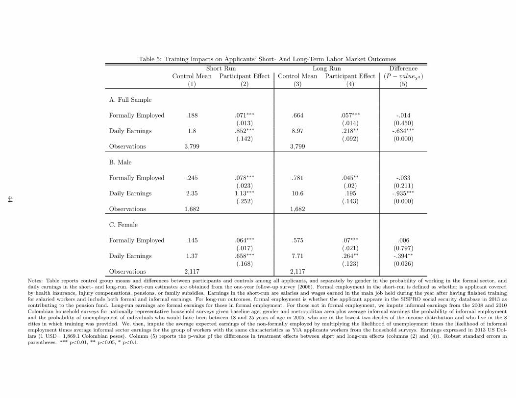


![Open Educational Resources (OER) Guide [FINAL].pdfThe term ‘Open Educational Resources’ (OER) describes any educational resources (including course materials, textbooks, videos,](https://static.documents.pub/doc/80x56/5ed1c9d8451b173a81390009/open-educational-resources-oer-guide-finalpdf-the-term-aopen-educational.jpg)


