Page 1
NBO 6.0 Program Manual
Natural Bond Orbital
Analysis Programs
compiled and edited by
Frank Weinhold and Eric D. Glendening
F. Weinhold: Theoretical Chemistry Institute and Department of Chemistry, University of
Wisconsin, Madison, Wisconsin 53706
E-mail: [email protected]
Phone: (608)262-0263
E. D. Glendening: Department of Chemistry and Physics, Indiana State University, Terre
Haute, Indiana 47809
E-mail: [email protected]
Phone: (812)237-2235
NBO6 Website: http://nbo6.chem.wisc.edu/
(c) Copyright 1996-2015 Board of Regents of the University of Wisconsin System on
behalf of the Theoretical Chemistry Institute. All Rights Reserved.
Page 2
i
Table of Contents
Table of Contents i
Preface: HOW TO USE THIS MANUAL v
Table 1: NBO Keyword/Keylist Quick Summary vi
A. GETTING STARTED
A.1 INTRODUCTION TO THE NBO 6.0 PROGRAM A-1
A.1.1 What Does the NBO Program Do? A-1
A.1.2 Input and Output A-4
A.1.3 General Capabilities and Restrictions A-6
A.1.4 References and Relationship to Previous Versions A-7
A.1.5 What's New in NBO 6.0? A-10
A.2 INSTALLING THE NBO PROGRAM A-14
A.3 TUTORIAL EXAMPLE FOR METHYLAMINE A-16
A.3.1 Running the Example A-16
A.3.2 Natural Population Analysis A-18
A.3.3 Natural Bond Orbital Analysis A-21
A.3.4 NHO Directional Analysis A-26
A.3.5 Perturbation Theory Energy Analysis A-27
A.3.6 NBO Summary A-22
B. NBO USER'S GUIDE
B.1 INTRODUCTION TO THE NBO USER'S GUIDE AND NBO KEYLISTS B-1
B.2 THE $NBO KEYLIST B-3
B.2.1 Overview of $NBO Keywords B-3
B.2.2 Job Control Keywords and Parameter Bracket Lists B-5
B.2.3 Job Threshold Keywords B-7
B.2.4 Matrix Output Keywords B-9
B.2.5 Other Output Control Keywords B-14
B.2.6 Print Level Keywords B-15
B.2.7 Semi-Documented Additional Keywords B-16
B.3 THE $CORE LIST B-18
B.4 THE $CHOOSE KEYLIST (DIRECTED NBO SEARCH) B-20
B.5 THE $DEL KEYLIST (NBO ENERGETIC ANALYSIS) B-23
B.5.1 Introduction to NBO Energetic Analysis B-23
B.5.2 The Nine Deletion Types B-25
B.5.3 Input for UHF Analysis B-29
B.6 NBO ILLUSTRATIONS B-31
B.6.1 Introduction B-31
B.6.2 NLMO Keyword B-32
B.6.3 DIPOLE Keyword B-34
B.6.4 Matrix Output Keywords B-36
B.6.5 BNDIDX Keyword B-39
B.6.6 Strong Delocalization: Benzene B-42
B.6.7 NOBOND Keyword: Hydrogen Fluoride B-46
Page 3
ii
B.6.8 Hypovalent Bonding: Diborane B-49
B.6.9 NBO Directed Search ($CHOOSE Keylist) B-53
B.6.10 NBO Energetic Analysis ($DEL Keylist) B-56
B.6.11 Open-Shell UHF Output: Methyl Radical B-59
B.6.12 Effective Core Potential: Cu2 Dimer B-63
B.7 FILE47: INPUT FOR THE GenNBO STAND-ALONE NBO PROGRAM B-68
B.7.1 Introduction B-68
B.7.2 Format of FILE47 B-69
B.7.3 $GENNBO Keylist B-71
B.7.4 $COORD Keylist B-73
B.7.5 $BASIS Datalist B-74
B.7.6 $CONTRACT Datalist B-76
B.7.7 $WF Datalist B-78
B.7.7 Matrix Datalists B-78
B.8 NRT: NATURAL RESONANCE THEORY ANALYSIS B-80
B.8.1 Introduction: Single and Multi-Reference NRT Analysis B-80
B.8.2 NRT Job Control Keywords B-84
B.8.3 Auxiliary $NRTSTR Keylist Input B-86
B.8.4 NRT Illustrations B-88
B.9 NBBP: NATURAL BOND-BOND POLARIZABILITY INDICES B-104
B.9.1 Introduction to NBBP B-104
B.9.2 NBBP Keyword Usage and Sample Output B-105
B.10 STERIC: NATURAL STERIC ANALYSIS B-108
B.10.1 Introduction to Natural Steric Analysis B-108
B.10.2 STERIC Keyword Usage and Sample Output B-110
B.11 NEDA: NATURAL ENERGY DECOMPOSITION ANALYSIS B-113
B.11.1 Introduction To NEDA B-113
B.11.2 Running NEDA in the NBO Framework B-115
B.11.3 Sample NEDA Input B-119
B.11.4 Sample NEDA Output B-124
B.12 CHECKPOINTING OPTIONS B-137
B.12.1 Introduction B-137
B.12.2 Checkpointing Options B-138
B.12.3 Checkpoint Permutation Lists B-140
B.12.4 Example: CAS/NBO and CI/NBO Calculations B-143
B.13 CMO: CANONICAL MO ANALYSIS B-144
B.13.1 Introduction B-144
B.13.2 CMO Keyword Usage and Sample Output B-145
B.14 NCS: NATURAL CHEMICAL SHIELDING ANALYSIS B-148
B.14.1 Introduction to Natural Chemical Shielding Analysis B-148
B.14.2 NCS Keyword Usage B-151
B.14.3 NCS Sample Output B-154
B.15 NJC: NATURAL J-COUPLING ANALYSIS B-157
B.15.1 Introduction to Natural J-Coupling Analysis B-157
B.15.2 NJC Keyword Usage B-163
B.15.3 NJC Sample Output B-165
Page 4
iii
B.16 3-CENTER, 4-ELECTRON HYPERBOND SEARCH B-168
B.16.1 Introduction B-168
B.16.2 Sample Output B-170
B.17 NBCP: NATURAL BOND CRITICAL POINT ANALYSIS B-172
B.17.1 Introduction to Natural Bond Critical Point Analysis B-172
B.17.2 NBCP Keyword Usage B-175
B.17.3 Additional NBCP_BP and NBCP_PT Keyword Options B-177
B.17.4 NBCP Sample Output B-178
B.18 NCE: NATURAL COULOMB ELECTROSTATICS ANALYSIS B-183
B.18.1 Introduction B-183
B.18.2 NCE Keyword Usage and Sample Output B-185
B.19 NCU: NATURAL CLUSTER UNIT ANALYSIS B-187
B.19.1 Introduction to NCU Analysis B-187
B.19.2 NCU Sample Output B-189
B.20 PROP: GENERAL 1E PROPERTY ANALYSIS B-191
B.21 MATRIX: GENERAL MATRIX OPERATOR AND
TRANSFORMATION OUTPUT
B-194
B.22 STRUCTURAL AND GRAPHICAL OUTPUT KEYWORDS B-197
B.23 EFFECTIVELY UNPAIRED ELECTRON DISTRIBUTION B-201
Page 5
iv
PREFACE: HOW TO USE THIS MANUAL
The NBO6 Manual consists of three major divisions:
Section A (“Getting Started”) contains introductory and one-time information
for the novice user – what the program does, new program functionality,
program installation, and a brief tutorial on sample output.
Section B (“NBO User's Guide”) is for the experienced user who has an
installed program and general familiarity with standard default NBO output.
This section documents the many keywords that can be used to alter and extend
standard NBO job options, with examples of the resulting output. Section B is
mandatory for users who wish to use the program to its full potential. This
section describes keyword-controllable capabilities of the basic NBO modules
(Sec. B.1-B.6) and GenNBO stand-alone program (Sec. B.7), as well as NBO-
based supplemental modules (Sec. B.8 et seq.).
Section C (“NBO Programmer's Guide”) is for accomplished programmers who
are interested in program logic and detailed source code. This section describes
the relationship of the source code subprograms to published algorithms,
providing documentation at the level of individual program parameters,
common blocks, functions, and subroutines. This in turn serves as a bridge to
the micro-documentation included as comment statements within the source
code. Section C also provides guidelines for constructing interface routines to
attach the NBO6 to new electronic structure packages.
The Appendices provide information on specific NBO versions (for Gaussian,
GAMESS,...), with details of installation and sample input files for individual
electronic structure systems.
The NBO website <http://nbo6.chem.wisc.edu/> provides additional tutorials,
sample input and output for main program keywords, and explanatory
background and bibliographic material to supplement this Manual.
A quick-reference index to NBO keywords and keylists discussed in this
manual is presented in Table 1 below. The table lists default (in [brackets]) and
optional keywords, indicating whether additional parameters must be provided
(Parms? Y = yes; N = no; opt. = optional) with a brief summary of the keyword
result and the page number of the Manual for further reference.
Page 6
v
Table 1: NBO Keyword/Keylist Quick Summary
Keyword Parms? Keyword Description Page
Main Program
Options
[BEND] opt. Hybrid directionality and “bond-bending”
analysis
A-26
CMO opt. Bonding character of canonical molecular orbitals B-144
DIPOLE opt. Dipole moment analysis B-34
[E2PERT] opt. 2nd-order perturbative estimates of NBO
interactions
A-27
MATRIX Y General operator and transformation matrix B-193
MEMORY Y Allocate dynamic memory B-6
NBBP opt. Natural bond-bond polarizability indices B-104
NBCP N Natural bond critical point analysis B-172
[NBO] N Natural bond orbital compositions A-21
[NBOSUM] N NBO summary table A-22
NCE N Natural coulomb electrostatics analysis B-183
NCS opt. Natural chemical shielding analysis B-148
NCU opt. Natural cluster unit analysis B-186
NEDA opt. Natural energy decomposition analysis B-113
NJC opt. Natural J-coupling analysis B-157
NLMO N Natural localized molecular orbital compositions B-32
[NPA] N Natural population analysis A-18
NRT N Natural resonance theory analysis B-80
PROP Y General 1e property analysis B-190
RADICAL N Effectively unpaired electron distribution B-201
STERIC opt. Natural steric analysis B-108
Control Options
AOINFO N Write AO basis information to LFN 31 B-14
Page 7
vi
ARCHIVE opt. Write ARCHIVE (FILE47) for stand-alone
GenNBO input
B-68
BNDIDX N NAO-Wiberg Bond Index and related valency
indices
B-39
BOAO opt. Fock-Dirac density matrix (“Bond order matrix”) B-16
CYCLES Y Limit cycles in NBO search B-16
DETAIL N Additional details of NBO search B-16
DIST N Atomic distance table B-14
FILE Y Specify filestem for PLOT files and other I/O B-14
FIXDM N Correct unphysical occupancies of input density
matrix
B-17
MATRIX Y Print general matrix operator output B-193
MOLDEN opt. Write geometry and orbitals in Molden format B-199
MOLUNIT Y User-specified molecular units B-6
MSPNBO N Maximum Spin-Paired NBOs (spin-averaged
density matrix)
B-5
MULAT N Gross Mulliken populations, by atom B-16
MULORB N Gross Mulliken populations, by orbital and atom B-16
NBOCML opt. Write NLS in CML format B-197
NBODAF opt. Write NBO direct access file (DAF) to disk B-16
NBOMOL opt. Write NLS in MDL format B-198
NOBOND N 1-center atomic hybrids (no 2-c NBO search) B-46
NRTCHG Y Alter maximum formal charge for candidate NRT
structures
B-84
NRTCML N Write NRT resonance structures in CML format B-198
NRTDTL N Additional details of NRT search B-84
NRTFDM N Use full density matrix for multi-reference NRT B-85
NRTLST Y Print leading $NRTSTR structure specifications B-84
NRTMEM Y Specify maximum number of NRT reference
structures (deprecated; see NRTREF)
B-84
Page 8
vii
NRTMOL opt. Write NRT resonance structures in MDL molfile
format
B-199
NRTOPT Y Specify alternative NRT optimization method B-85
NRTTHR Y Specify delocalization threshold for NRT search B-84
NRTWGT Y Alter weighting threshold for NRT reference
structure
B-85
PLOT N Write files for orbital plotting B-14
PRINT Y Heirarchical print control of NBO output B-15
PRJTHR Y Alter projection threshold for NHO search B-16
PROP Y NBO/NLMO analysis of selected operators B-190
RPNAO N Revised pure AO (PAO) to PNAO transformation B-16
SKIPBO N Skip NBO search (NPA only for PRINT=1) B-5
SVEC opt. Print eigenvectors of AO overlap matrix B-17
THRESH Y Alter occupancy threshold for NBO search B-16
XMOL opt. Write XMol-formatted geometry B-199
Operator Matrix
Output
DI opt. Output dipole moment matrix (DIAO, DINAO,
etc.)
B-9
DM opt. Output density matrix (DMAO, DMNAO, etc.) B-9
F opt. Output Fock matrix (FAO, FNAO, etc.) B-9
K opt. Output kinetic energy matrix (KAO, KNAO, etc.) B-9
S opt. Output overlap matrix (SAO, SPNAO, SPNBO,
SPNLMO)
B-9
V opt. Output 1-e (N-e attraction) potential matrix
(VAO, VNAO, etc.)
B-9
Transformation
Matrix Output
AOPAO opt. Output AO to PAO transformation B-9
AONAO opt. Output AO to NAO transformation B-9
AOPNAO opt. Output AO to PNAO transformation B-9
Page 9
viii
AONHO opt. Output AO to NHO transformation B-9
AOPNHO opt. Output AO to PNHO transformation B-9
AONBO opt. Output AO to NBO transformation B-9
AOPNBO opt. Output AO to PNBO transformation B-9
AONLMO opt. Output AO to NLMO transformation B-9
AOPNLMO opt. Output AO to PNLMO transformation B-9
AONO opt. Output AO to NO transformation B-9
AOMO opt. Output AO to MO (LCAO-MO) transformation B-9
PAOPNAO opt. Output PAO to PNAO transformation B-16
NAONHO opt. Output NAO to NHO transformation B-9
NAONBO opt. Output NAO to NBO transformation B-9
NAONLMO opt. Output NAO to NLMO transformation B-9
NAONO opt. Output NAO to NO transformation B-9
NAOMO opt. Output NAO to MO transformation B-9
NHONBO opt. Output NHO to NBO transformation B-9
NHONLMO opt. Output NHO to NLMO transformation B-9
NHONO opt. Output NHO to NO transformation B-9
NHOMO opt. Output NHO to MO transformation B-9
NBONLMO opt. Output NBO to NLMO transformation B-9
NBONO opt. Output NBO to NO transformation B-9
NBOMO opt. Output NBO to MO transformation B-9
NLMONO opt. Output NLMO to NO transformation B-9
NLMOMO opt. Output NLMO to MO transformation B-9
NOMO opt. Output NO to MO transformation B-9
Auxiliary
Keylists
$CHOOSE Y Specify alternative Lewis structure for NBO
search
B-20
$CORE Y Modify default NBO core table B-18
Page 10
ix
$DEL Y Delete selected NBOs, interactions, or blocks of
interactions
B-23
$NRTSTR Y Specify reference structures for NRT analysis
(also $NRTSTRA and $NRTSTRB)
B-86
Auxiliary FILE47
Keylists
$BASIS Y Atomic centers and angular symmetries of AOs B-74
$C10 Y Derivative MO coefficients B-154
$CONTRACT Y Contraction coefficients and orbital exponents of
AOs
B-76
$COORD Y Job title, atoms, Cartesian coordinates B-73
$DENSITY Y Density matrix in AO basis B-69
$DIPOLE Y Dipole matrix in AO basis B-69
$FOCK Y Fock matrix in AO basis B-69
$GENNBO Y Specify calculation model size, type and units B-71
$H01 Y GIAO Hamiltonian first derivatives B-154
$H11 Y GIAO Hamiltonian second derivativies B-154
$KINETIC Y Kinetic energy matrix in AO basis B-69
$LCAOMO Y Canonical MOs in AO basis B-69
$NUCLEAR Y Nuclear-electron attraction matrix in AO basis B-69
$OVERLAP Y Overlap matrix in AO basis B-69
Page 11
A.1 INTRODUCTION TO THE NBO 6.0 PROGRAM
A-1
Section A: GETTING STARTED
A.1 INTRODUCTION TO THE NBO 6.0 PROGRAM
A.1.1 What Does the NBO Program Do?
The NBO program performs the analysis of a many-electron molecular
wavefunction in terms of localized electron-pair bonding units. The program
carries out the determination of natural atomic orbitals (NAOs), natural hybrid
orbitals (NHOs), natural bond orbitals (NBOs), and natural localized molecular
orbitals (NLMOs), and uses these to perform natural population analysis
(NPA), NBO energetic (deletions) analysis, and other tasks pertaining to
localized analysis of wavefunction properties, including natural resonance
theory (NRT) and natural chemical shielding (NCS) analysis. This section
provides a brief introduction to NBO algorithms and nomenclature.
The NBO method makes use of only the first-order reduced density matrix of
the wavefunction, and hence is applicable to wavefunctions of general
mathematical form. In the open-shell case, the analysis is performed in terms
of “different NBOs for different spins,” based on distinct density matrices for α
and β spin. [Note, however, that electronic structure packages may not provide
the spin density matrices for certain types of open-shell wavefunctions (e.g.,
MCSCF or CASSCF wavefunctions calculated by the GUGA formalism). In
this case NBO analysis can only be applied in the “maximum spin-paired”
(MSPNBO) formulation.]
NBO analysis is based on a method for optimally transforming a given
wavefunction into localized form, corresponding to the one-center (“lone pair”)
and two-center (“bond”) elements of the chemist's Lewis structure picture. The
NBOs are obtained as local block eigenfunctions of the density matrix, and are
hence “natural” in the sense of Löwdin, having optimal convergence properties
for describing the electron density. The set of high-occupancy NBOs, each
taken doubly occupied, is said to represent the “natural Lewis structure” (NLS)
of the molecule. Delocalization effects appear as weak departures from this
idealized localized picture. (For transition metals, a normal-valent Lewis-like
structure conforms to a dodectet rule, rather than the normal octet rule for
main-group elements.)
The various natural localized sets can be considered to result from a sequence
of transformations of the input atomic orbital basis set {χi},
input basis AOs → NAOs → NHOs → NBOs → NLMOs
Page 12
A.1 INTRODUCTION TO THE NBO 6.0 PROGRAM
A-2
[Note that the restriction to starting AOs is not intrinsic. If the wavefunction
were not calculated in an atom-centered basis, one could first compute
wavefunctions for the individual atoms (in the actual basis set and geometry of
the molecular calculation) and select the most highly occupied natural orbitals
as the starting “atomic orbitals” for that atom. Indeed, NBOs have now been
obtained for a variety of systems in the framework of plane-wave and related
grid-type descriptions; see B. Dunnington and J. R. Schmidt, “Generalization of
Natural Bond Orbital Analysis to Periodic Systems: Applications to Solids and
Surfaces via Plane-Wave Density Functional Theory,” J. Chem. Theor. Comp.
8, 1902 (2012); L. P. Lee, D. J. Cole, M. C. Payne, and C.-K. Skylaris, “Natural
Bond Orbital Analysis in Linear-Scaling Density Functional Theory
Calculations” <http://www2.tcm.phy.cam.ac.uk/onetep/Focus/
BiologicalApplications>. However, because atom-centered basis functions are
the nearly universal choice for molecular calculations, the NBO6 program
makes no provision for this step.]
Each natural localized set forms a complete orthonormal set of one-electron
functions for expanding the delocalized molecular orbitals (MOs) or forming
matrix representations of one-electron operators. The overlap of associated
“pre-orthogonal” NAOs (PNAOs), lacking only the interatomic
orthogonalization step of the NAO procedure, can be used to estimate the
strength of orbital interactions in the usual way, based on Mulliken-type
approximations.
The optimal condensation of occupancy in the natural localized orbitals leads to
partitioning into high- and low-occupancy orbital types (reduction in
dimensionality of the orbitals having significant occupancy), as reflected in the
orbital labelling. The small set of most highly-occupied NAOs, having a close
correspondence with the effective minimal basis set of semi-empirical quantum
chemistry, is referred to as the “natural minimal basis” (NMB) set. The NMB
(core + valence) functions are distinguished from the weakly occupied
“Rydberg” (extra-valence-shell) functions that complete the span of the NAO
space, but typically make little contribution to molecular properties. Similarly
in the NBO space, the highly occupied NBOs of the natural Lewis structure
(NLS) can be distinguished from the “non-Lewis” antibond and Rydberg
orbitals that complete the span of the NBO space. Each pair of valence hybrids
hA, hB in the NHO basis give rise to a bond (σAB) and antibond (σ*AB) in the
NBO basis,
σAB = cAhA + cBhB
σ*AB = cBhA − cAhB
Page 13
A.1 INTRODUCTION TO THE NBO 6.0 PROGRAM
A-3
the former a Lewis (L, occupied) and the latter a non-Lewis (NL, unoccupied)
orbital. The antibonds (valence shell non-Lewis orbitals) typically play the
primary role in departures (delocalization) from the idealized Lewis structure.
The NBO program also makes extensive provision for energetic analysis of
NBO interactions, based on the availability of a 1-electron effective energy
operator (Fock or Kohn-Sham matrix) for the system. [As noted above, the
construction of NAOs and NBOs is wholly independent of any such energy
operator (or geometry) information.] Estimates of energy effects are based on
second-order perturbation theory, or on the effect of deleting certain orbitals or
matrix elements and recalculating the total energy. NBO energetic analysis is
dependent on the host electronic structure system (ESS) to which the NBO
program is attached, as described in the Appendix. Analysis of a DFT
calculation is performed analogously to a Hartree-Fock calculation, but uses
Kohn-Sham orbitals that incorporate important effects of a correlated electronic
distribution that are displayed in details of the NAOs, NBOs, and their
occupancies.
NBO 6.0 includes NBO-based supplementary modules for performing natural
resonance theory (NRT) analysis, natural bond-bond polarizability (NBBP)
evaluation, natural steric analysis, natural energy decomposition analysis
(NEDA), and natural bond critical point (NBCP) analysis. New features of
NBO 6.0 include modules for analyzing NMR chemical shielding tensors and J-
coupling constants as well as improved localized description of canonical MO
composition. The supplementary modules build on and extend the capabilities
of core NBO analysis, and are described separately in Sections B.8 et seq.
NBO 6.0 comes installed in a number of leading ESS packages, and one should
follow the instructions provided with the ESS on how to run NBO. The NBO
program can also be obtained as a binary or source code distribution that, in
principle, can be attached to any ESS of the user's choice. In addition, specific
interface routines are provided that facilitate the attachment to a number of
popular ab initio packages (Gaussian, GAMESS, Molpro).
Page 14
A.1 INTRODUCTION TO THE NBO 6.0 PROGRAM
A-4
A.1.2 Input and Output
From the user's point of view, input to the NBO portion of an ESS/NBO
program consists simply of one or more keywords enclosed in NBO keylists in
the ESS input file. The main NBO keylist (the $NBO keylist) is of the form:
$NBO ...(keywords)... $END
Simple examples of such $NBO keylists are
$NBO dipole nrt $END
$NBO file=myjob archive naonbo ncs=0.05 $END
Note that keylists are always delimited with $-prefixed identifiers: an identifier
such as $NBO to open the keylist and $END to terminate it. Keylist delimiters
and keywords are case-insensitive, and the keylist can extend across multiple
lines, e.g.
$nbo
file=/home/me/nbo6/myjob
ARCHIVE
naonbo
ncs=0.05,csa
$end
Other keylist identifiers include $CORE, $CHOOSE, $NRTSTR, and $DEL.
Keylists cannot be nested, and each new keylist must begin on a new line. The
NBO program reads the keywords of each keylist to set various job options,
then interrogates the ESS program for information concerning the
wavefunction to perform the requested tasks.
Common abbreviations used in naming keywords are:
S Overlap matrix
DM Density matrix
F Fock or Kohn-Sham matrix
K Kinetic energy matrix
V 1-electron potential energy (nuclear-electron attraction) matrix
DI Dipole matrix
NPA Natural population analysis
NAO Natural atomic orbital
NHO Natural hybrid orbital
NBO Natural bond orbital
NLMO Natural localized molecular orbital
Page 15
A.1 INTRODUCTION TO THE NBO 6.0 PROGRAM
A-5
PNAO pre-orthogonal NAO (omit interatomic orthogonalization)
PNHO pre-orthogonal NHO (formed from PNAOs)
PNBO pre-orthogonal NBO (formed from PNAOs)
PNLMO pre-orthogonal NLMO (formed from PNAOs)
The general form of NBO keylists and the specific functions associated with
each keyword are detailed in the User's Guide, Section B. The particular way
of including NBO keylists in the input file for each ESS is detailed in the
appropriate section of the Appendix.
Principal output from the NBO program consists of the tables and summaries
describing the results of NBO analysis, generally written to the ESS output file.
Sample default NBO output is described in Section A.3, and sample output for
many NBO keyword options is presented in Sec. B.6 and the individual
sections for NBO supplementary modules (Sec. B.8 et seq).
The NBO program writes transformation matrices and other data to disk files.
Two particularly noteworthy files are the NBO direct-access file (FILE48) that
the program uses to store intermediate results during a calculation, and the
archive file (FILE47) that, written on request, can be used with the stand-alone
GenNBO program to repeat NBO analysis without running the ESS program to
recalculate the wavefunction. Details of FILE47 and FILE48 are given in
Section B.7 and the Programmer's Guide, Section C.
Page 16
A.1 INTRODUCTION TO THE NBO 6.0 PROGRAM
A-6
A.1.3 General Capabilities and Restrictions
Principal capabilities of the NBO program are:
(1) Natural population, natural bond orbital, and natural localized molecular
orbital analysis of densities from SCF, Moller-Plesset, MCSCF, CI, coupled
cluster, and density functional calculations;
(2) For HF/DFT methods only, energetic analysis of the wavefunction in terms
of the interactions (Fock or Kohn-Sham matrix elements) between NBOs;
(3) Localized analysis of molecular dipole moments in terms of NLMO and
NBO bond moments and their interactions;
(4) Additional analyses provided by NBO-based supplemental modules (Sec.
B.8 et seq.), including natural resonance theory, natural steric analysis, bond-
bond polarizability indices, natural chemical shielding analysis, natural J-
coupling analysis, and natural energy decomposition analysis. New features of
NBO 6.0 are summarized in Sec. A.1.5.
Most NBO storage is allocated dynamically to conform to the minimum
required for the molecular system under study. However, certain NBO
common blocks of fixed dimensionality are used for storage. These are
currently dimensioned to accommodate up to 500 atoms and 5000 basis
functions. Section C.3 describes how these restrictions can be altered. The
program is not set up to handle complex wavefunctions, but can treat any real
RHF, ROHF, UHF, MCSCF (including GVB), CI, CC, or Moller-Plesset-type
wavefunction (i.e., any form of wavefunction for which the requisite density
matrices are available) for ground or excited states of general open- or closed-
shell molecules. Effective core potentials (“pseudopotentials”) can be handled,
including complete neglect of core electrons as assumed in semi-empirical
treatments. The atomic orbital basis functions (including Cartesian spdfgh and
spherical spdfghi functions in angular symmetry) may be of general Slater-type,
contracted Gaussian-type, or other general composition, including the
“effective” orthonormal valence-shell AOs of semi-empirical treatments. AO
basis functions are assumed to be normalized, but in general non-orthogonal.
Linear dependence is handled by discarding subshells of offending functions.
Page 17
A.1 INTRODUCTION TO THE NBO 6.0 PROGRAM
A-7
A.1.4 References and Relationship to Previous Versions
The NBO 6.0 program should be cited as follows:
NBO 6.0. E. D. Glendening, J. K. Badenhoop, A. E. Reed, J. E. Carpenter, J.
A. Bohmann, C. M. Morales, C. R. Landis, and F. Weinhold, Theoretical
Chemistry Institute, University of Wisconsin, Madison (2013).
NBO 6.0 is an extension of previous versions of the NBO method:
(1) “Version 1.0,” the semi-empirical version incorporated in program
BONDO and distributed through the Quantum Chemistry Program Exchange
[F. Weinhold, Quantum Chemistry Program Exchange No. 408 (1980)];
(2) “Version 2.0,” the first ab initio implementation, designed for interfacing
with Gaussian-82 and distributed through QCPE [A. E. Reed and F. Weinhold,
QCPE Bull. 5, 141 (1985)];
(3) Version 3.0, the general-purpose ab initio implementation developed for
distribution through QCPE, and soon incorporated (as “Version 3.1”) into
commercial Gaussian distributions [E. D. Glendening, A. E. Reed, J. E.
Carpenter, and F. Weinhold, QCPE Bull. 10, 58 (1990)];
(4) Version 4.0, the subsequent UW/TCI version (under copyright of the
University of Wisconsin, Madison) that added NRT, STERIC, NEDA, and
other capabilities [NBO 4.0. E. D. Glendening, J. K. Badenhoop, A. E. Reed, J.
E. Carpenter, and F. Weinhold, Theoretical Chemistry Institute, University of
Wisconsin, Madison (1996)];
(5) Version 5.0, the long-running UW/TCI version that maintained link-ready
connectivity to leading ESS host systems and added CMO, NCS, NJC, 3CHB,
and other capabilities [NBO 5.0. E. D. Glendening, J. K. Badenhoop, A. E.
Reed, J. E. Carpenter, J. A. Bohmann, C. M. Morales, and F. Weinhold
(Theoretical Chemistry Institute, University of Wisconsin, Madison, WI,
2001)].
NBO 6.0 should be considered to supercede those versions, as well as interim
revisions and extensions of NBO 5.0, such as NBO 5.X, NBO 5.G, and NBO
5.9.
Page 18
A.1 INTRODUCTION TO THE NBO 6.0 PROGRAM
A-8
Principal contributors (1975-2015) to the conceptual development of the NBO
methods contained in this program are
T. K. Brunck J. P. Foster
A. B. Rives A. E. Reed
R. B. Weinstock J. E. Carpenter
E. D. Glendening J. K. Badenhoop
J. A. Bohmann S. J. Wilkens
C. M. Morales C. R. Landis
F. Weinhold
Others who contributed to program development or technical implementation
of individual program segments include S. Baker, J. K. Blair, S. H. Feldgus, T.
C. Farrar, J. L. Markley, J. Michl, A. V. Nemukhin, A. Streitwieser, W. M.
Westler, and H. E. Zimmerman. Many other colleagues and co-workers have
provided useful comments and suggestions that are reflected in the final version
of the program, and for which we are grateful.
References to the development and applications of principal
NAO/NBO/NLMO methods include:
Natural Bond Orbitals:
J. P. Foster and F. Weinhold, J. Am. Chem. Soc. 102, 7211-7218 (1980)
Natural Atomic Orbitals and Natural Population Analysis:
A. E. Reed and F. Weinhold, J. Chem. Phys. 78, 4066-4073 (1983)
A. E. Reed, R. B. Weinstock, and F. Weinhold, J. Chem. Phys. 83, 735-746
(1985)
Natural Localized Molecular Orbitals:
A. E. Reed and F. Weinhold, J. Chem. Phys. 83, 1736-1740 (1985)
Open-Shell NBO:
J. E. Carpenter and F. Weinhold, J. Molec. Struct. (Theochem) 169, 41-62
(1988)
Comprehensive Review Articles:
Page 19
A.1 INTRODUCTION TO THE NBO 6.0 PROGRAM
A-9
A. E. Reed, L. A. Curtiss, and F. Weinhold, Chem. Rev. 88, 899-926 (1988)
F. Weinhold, “Natural Bond Orbital Methods,” In, Encyclopedia of
Computational Chemistry P. v.R. Schleyer, N. L. Allinger, T. Clark, J.
Gasteiger, P. A. Kollman, H. F. Schaefer III, P. R. Schreiner (Eds.), (John
Wiley & Sons, Chichester, UK, 1998), Vol. 3, pp. 1792-1811
E. D. Glendening, C. R. Landis and F. Weinhold, “Natural Bond Orbital
Methods,” WIREs Comp. Mol. Sci. 2, 1-42 (2012)
F. Weinhold, “Natural bond orbital analysis: A critical overview of
relationships to alternative bonding perspectives,” J. Comput. Chem. (2012).
Books:
F. Weinhold and C. R. Landis, Valency and Bonding: A Natural Bond Orbital
Donor-Acceptor Perspective (Cambridge U. Press, 2004), 760pp.
F. Weinhold and C. R. Landis, Discovering Chemistry with Natural Bond
Orbitals (Wiley-VCH, 2012), 319pp.
Leading references for NBO-based supplementary modules are included in
Sections B.8 et seq. Further background and bibliographic materials can be
found on the NBO website: <http://nbo6.chem.wisc.edu/biblio_css.htm>
Page 20
A.1 INTRODUCTION TO THE NBO 6.0 PROGRAM
A-10
A.1.5. What's New in NBO 6.0?
NBO 6.0 introduces deep structural, algorithmic, and notational changes from
previous versions of the NBO program, as well as a variety of new analysis
modules (described below) that add to the power and versatility of general
NBO analysis technology. We describe in turn the leading changes of each
type:
Structural Programming Changes
NBO 6.0 inaugurates a fundamentally new programming model for interacting
with a host electronic structure system (ESS). For suitable “NBO6-
compatible” ESS host programs (<http://nbo6.chem.wisc.edu/affil_css.htm>),
NBO 6.0 is provided as a binary executable (nbo6.exe) that cooperates
interactively with the host ESS program through a direct message-passing
protocol, without linking into an integrated binary (as required in previous
ESS/NBO5 implementations).
Practically speaking, the new-style unlinked ESS/NBO6 has both similar
capabilities and similar “look and feel” as older linked ESS/NBO5 versions –
including $DEL-deletions, NEDA, NCS, NJC, CAS/NBO, and other interactive
options. However, such two-way interactivity is now achieved at “arms
length” by a binary-to-binary communication protocol that avoids technical,
commercial, and legal complications of older linked versions.
NBO 6.0 is still provided in source code form. The source can be used to
generate the stand-alone GenNBO program (gennbo.exe) that accepts input
from NBO archive (FILE47) files, as produced by many current ESS programs.
One can also generate binaries (message-passing nbo6.exe) for alternative
OS/hardware configurations or NBO6-compatible ESS host systems. NBO 6.0
source cannot be used to create old-style linked ESS/NBO binaries.
Algorithmic Changes
NBO 6.0 introduces important algorithmic improvements that will scarcely be
noticable in applications to common chemical species, but significantly
improve the consistency, generality, and reliability of NBO analysis for more
exotic excited-state and multi-center species. These improvements also
underlie new analysis options and notational conventions to be described
below.
Page 21
A.1 INTRODUCTION TO THE NBO 6.0 PROGRAM
A-11
(1) In former versions of the sequential search for one- and two-center NBOs,
a simple “depletion” procedure was used to (approximately) remove 1c
contributions from the NAO density matrix prior to 2c search, with small errors
subsequently removed by symmetric orthogonalization. Depletion has now
been replaced by strict orthogonal projection (annihilation) to insure rigorous
orthonormality at each step of the multi-center search sequence.
(2) In former versions of the search for high-occupancy NBOs, the “pair”
occupancy threshold was decremented over a coarse grid (1.90, 1.80,...,1.50)
that sometimes allowed a superior natural Lewis structure to be skipped over in
strongly delocalized systems. The revised NBO 6.0 search uses a more
sophisticated threshold decrement algorithm to thoroughly explore possible
NLS bonding patterns. Compared to the older algorithm, this corresponds to a
finer grid search and insures, at the theorem level, that the optimal NLS has
been found, The newer algorithm is usually more efficient as well.
Notational and Organizational Output Changes
Two principal changes in the notation and organization of NBO output will be
evident to the experienced NBO user:
(1) In former NBO output, a star(*)-label (such as BD*, LP*, RY*, 3C*) was
conventionally taken to identity NL-type “excited” NBOs of low occupancy,
which provide small delocalization corrections to the highly occupied
"unstarred" L-type NBOs of the formal NLS configuration. However, a star-
label is also conventionally used to identify out-of-phase ("antibonding")
symmetry of a 2-center orbital about an inversion center or reflection plane, or
an analogous more highly-noded phase pattern of a multi-center orbital. The
ambiguities of using “*” to connote both “excitation” and “out-of-phase
symmetry” are consistent with common chemical usage, and present no
apparent difficulties for conventional 2-center NLS bonding patterns of ground
state species. However, such ambiguities lead to increasing conflicts for the
exotic multi-center bonding scenarios of excited-state or metallic species,
mandating more restricted usage of star-labels in NBO 6.0.
Gross inconsistencies arise whenever an out-of-phase "BD*" orbital is found to
be of higher occupancy than the corresponding in-phase "BD" orbital, thereby
forcing reversal of the usual assignments of L vs. NL labels. In such cases,
earlier NBO versions printed a warning message ("apparent excited-state
configuration encountered...") and reassigned "BD" vs. "BD*" labels according
to phase-pattern rather than occupancy order. This leads to superficially large
NL-density and (often) to grossly sub-optimal NBOs and NLS assignments.
Page 22
A.1 INTRODUCTION TO THE NBO 6.0 PROGRAM
A-12
Although rare for ground-state species, such cases become increasingly
common in excited states.
NBO 6.0 avoids these notational conflicts by more clearly distinguishing L-type
and NL-type NBOs in separated output sections, removing any presumed
association with “*” labels. Instead, the "*" label is reserved primarily for the
more traditional chemical association with out-of-phase (“antibonding”)
character of 2c/2e (“BD*” type) or 3c/2e (“3C*” type) NBOs, and secondarily
for the distinctive “LP*” (unfilled valence-shell nonbonding) NBOs of
hypovalent species (following usage established in previous NBO program
versions). For common ground-state species, these notational changes have
practically no perceptible effect. However, a more comprehensive perspective
that includes excited-state and far-from-equilibrium species makes the need for
such changes increasingly apparent.
(2) In NBO 6.0 output, the ordering of NBOs is now altered to reflect the
actual multi-center search priority for L-type NBOs (1c < 2c < 3c) and
prioritized occupancy ordering for NL-type NBOs. As a result, the 1c core
(“CR”) and lone pair (“LP”) NBOs appear first, followed by 2c bonds (“BD”)
[and, if needed, 3c bonds (“3C”)] in the L-listing, while the formally empty 1c
valence orbitals (LP*), 2c valence antibonds (BD*) [and, if needed, 3-center
NL orbitals (3Cn and 3C*)] now precede the residual 1c Rydberg-type (RY)
NBOs in the NL-listing. As mentioned above, the clear delineation of Lewis
and non-Lewis sections of NBO output also departs from older format.
New Analysis Features and Options
NBO 6.0 includes major new capabilities related to multi-center bonding,
supramolecular aggregation, and L/NL decomposition of electrostatic and other
properties, as well as extensions and improvements of established NBO
analysis tools. Principal new NBO features include:
(1) Automatic Three-Center Bond Search. If the initial 1c/2c search leaves
unassigned NL-density exceeding the current occupancy threshold, the NBO
search automatically extends to 3-center NBOs. The former “3CBOND”
keyword is therefore deprecated, and hypovalent 3c/2e τ-bonds of borane-type
species are now recognized without user intervention. The corresponding
“3CHB” keyword for Pimentel-Rundle-Coulson-type 3c/4e interactions is also
deprecated, and such strong 2-resonance “hyperbonds” are now automatically
recognized by the program.
Page 23
A.1 INTRODUCTION TO THE NBO 6.0 PROGRAM
A-13
(2) Natural Coulomb Electrostatics Analysis (NCE Keyword). NPA atomic
charges for the idealized NLS and actual molecular charge distribution are
combined with interatomic distances to distinguish the classical-type (L) and
resonance-type (NL) contributions to apparent “Coulomb electrostatics.”
(3) Natural Cluster Unit Analysis (NCU Keyword). A general measure of
interaction strength (τNCU) is continuously varied to obtain the intrinsic “units”
or “building blocks” that are characteristic of aggegation in each range of
interatomic interactions, from the strong forces of chemical bonding to the
weak forces of London dispersion.
(4) General 1-Electron Property Analysis (PROP Keyword). A template is
provided for NBO analysis of any 1e property whose AO matrix elements are
provided by the host ESS program.
(5) General 1-Electron Property Matrix (MATRIX Keyword). A template is
provided for transforming the matrix elements of any available 1e property to
localized (NAO/NHO/NBO/NLMO) or delocalized (MO) basis form.
(6) “Local NRT” Options. New provision is made for constraining NRT
weighting to selected sub-units (resonance units) of the overall system, thus
allowing a “divide and conquer” strategy for overcoming convergence
difficulties of multiple resonating groups. Other algorithmic improvements
now allow efficient NRT description of many previously intractable species.
(7) NLS $CHOOSE Keylist Output. NBO summary output now includes a
corresponding $CHOOSE keylist specification (Sec. B.4) for the bonding
pattern of the final NLS.
Despite these changes and extensions, NBO 6.0 was designed to be compatible
with earlier versions as nearly as possible. Experienced NBO users should find
that familiar features run practically unchanged, providing the framework for a
smooth and intuitive migration to new keywords and features.
Page 24
A.3 TUTORIAL EXAMPLE FOR METHYLAMINE
A-14
A.2 INSTALLING THE NBO PROGRAM
[NBO 6.0 comes installed in a number of leading ESS packages. Users of these
packages may ignore this section.]
The NBO program is distributed in electronic download or CD form, either as
binary executables or source code. Installation instructions differ in these
cases. In either case, the final NBO6 binary executables are intended to
communicate interactively with a chosen NBO6-compatible host electronic
structure system (ESS) or with the GenNBO program that takes its input from
an archive (FILE47) file.
Windows Binary Executable Distribution
The Windows distribution includes the NBO6 executable (nbo6.i4.exe), the
GenNBO executable (gennbo.i4.exe), sample FILE47 input files, and a batch
script (gennbo.bat) for executing the sample calculations. Instructions for
installing and testing these executables are provided with the distribution.
Linux Binary Executable Distribution
Binary executable distributions are available for Linux operating systems,
including Cygwin and Mac OS-X. (Installation for other Unix-based operating
systems may require the source distribution described below.) The Linux
distribution includes the 32- and 64-bit integer NBO6 executables (nbo6.i4.exe
and nbo6.i8.exe), the GenNBO executables (gennbo.i4.exe and gennbo.i8.exe),
source code or libraries for installing NBO6 in Gaussian-09 and GAMESS,
sample FILE47 files, and a tcsh script (gennbo) for executing the sample
calculations. Instructions for installing and testing these executables are
provided with the distribution.
Source Code Distribution
The source distribution consists of the master NBO source code, GNU
makefiles, and utility routines for building 32- and 64-bit executables,
including the NBO6 executables (nbo6.i4.exe and nbo6.i8.exe) and GenNBO
executables (gennbo.i4.exe and gennbo.i8.exe) GNU, Portland Group, and
Intel Fortran compilers are fully supported by the distribution. Other compilers
may successfully build executables too, but are not currently supported by the
NBO development team. Consult the “Frequently Asked Questions” link of the
NBO6 website <http://nbo6.chem.wisc.edu/faq_css.htm> or contact the authors
if you encounter undue difficulties when building the NBO executables.
Page 25
A.3 TUTORIAL EXAMPLE FOR METHYLAMINE
A-15
The installation of the NBO programs into your host ESS system generally
does not affect the way your system processes standard input files. The only
change involves the reading of NBO keylists (if detected in your input file),
performance of the NBO tasks requested in the keylist, and return of control to
the ESS program in the state in which the NBO call was encountered (unless
checkpointing operations were performed; Sec. B.12).
You are encouraged to contact the authors when attempting to interface NBO
6.0 to an ESS package that is not currently supported by the source code
distribution. It may be possible for the authors to assist with this effort.
Alternatively, you might consider having the ESS write a FILE47 file that can
be used as input to the GenNBO stand-alone version of the NBO program. See
Section B.7 for a description of this file.
Page 26
A.3 TUTORIAL EXAMPLE FOR METHYLAMINE
A-16
A.3 TUTORIAL EXAMPLE FOR METHYLAMINE
A.3.1 Running the Example
This section provides an introductory quick-start tutorial on running a simple
NBO job and interpreting the output. The example chosen is that of
methylamine (CH3NH2) in Pople-Gordon idealized geometry, treated at the ab
initio RHF/3-21G level. Cartesian coordinates (in Angstroms) of the atoms at
this geometry are
C 0.745914 0.011106 0.000000
N -0.721743 -0.071848 0.000000
H 1.042059 1.060105 0.000000
H 1.129298 -0.483355 0.892539
H 1.129298 -0.483355 -0.892539
H -1.076988 0.386322 -0.827032
H -1.076988 0.386322 0.827032
corresponding to bond lengths of 1.47 (C-N), 1.09 (C-H), and 1.01 Å (N-H)
with tetrahedral bond angles and staggered dihedrals. The 3-21G split-valence
basis set consists of 28 AOs (nine each on C and N, two on each H), extended
by 13 AOs beyond the minimal basis level.
In many cases, you can modify the standard ESS input file to produce NBO
output by simply including the line
$NBO $END
at the end of the file. This is an empty NBO keylist, specifying that NBO
analysis should be carried out at the default level. Alternatively, GenNBO can
be run with the FILE47 archive file (ch3nh2.47) provided with the binary and
source distributions to produce the NBO output described here.
Default NBO output produced by this example is shown below, just as it
appears in your output file. The start of the NBO section is marked by a
standard header, citation, and job title:
N2
C1
H3
H4
H7
H6
H5
Page 27
A.3 TUTORIAL EXAMPLE FOR METHYLAMINE
A-17
*********************************** NBO 6.0 ***********************************
N A T U R A L A T O M I C O R B I T A L A N D
N A T U R A L B O N D O R B I T A L A N A L Y S I S
*************************** University of Wisconsin ***************************
(c) Copyright 1996-2014 Board of Regents of the University of Wisconsin System
on behalf of the Theoretical Chemistry Institute. All rights reserved.
Cite this program as:
NBO 6.0. E. D. Glendening, J. K. Badenhoop, A. E. Reed,
J. E. Carpenter, J. A. Bohmann, C. M. Morales, C. R. Landis,
and F. Weinhold (Theoretical Chemistry Institute, University
of Wisconsin, Madison, WI, 2013); http://nbo6.chem.wisc.edu/
Filename set to ch3nh2
Job title: Methylamine...RHF/3-21G//Pople-Gordon standard geometry
The NBO banner reports the program version (NBO 6.0) and license name
(“University of Wisconsin” in this case).
NBO output is formatted to maximum 80-character width for convenient
display on a computer terminal or printed page. The NBO heading echoes any
requested keywords (none for the present default case). The filename that is
reported (“ch3nh2” in this case) is used to open named files, such as the
FILE48 direct-access file (ch3nh2.48) and FILE47 archive file (ch3nh2.47).
(The latter is only produced when the user adds the ARCHIVE keyword to the
$NBO keylist.)
Page 28
A.3 TUTORIAL EXAMPLE FOR METHYLAMINE
A-18
A.3.2 Natural Population Analysis
The next four NBO output segments summarize the results of natural
population analysis (NPA). The first segment is the main NAO table, as shown
below:
NATURAL POPULATIONS: Natural atomic orbital occupancies
NAO Atom No lang Type(AO) Occupancy Energy
---------------------------------------------------------
1 C 1 s Cor( 1s) 1.99901 -11.04148
2 C 1 s Val( 2s) 1.09144 -0.28255
3 C 1 s Ryd( 3s) 0.00067 1.95637
4 C 1 px Val( 2p) 0.88696 -0.01597
5 C 1 px Ryd( 3p) 0.00142 0.93152
6 C 1 py Val( 2p) 1.21481 -0.07285
7 C 1 py Ryd( 3p) 0.00063 1.02989
8 C 1 pz Val( 2p) 1.24537 -0.08879
9 C 1 pz Ryd( 3p) 0.00056 1.01733
10 N 2 s Cor( 1s) 1.99953 -15.25896
11 N 2 s Val( 2s) 1.42760 -0.71766
12 N 2 s Ryd( 3s) 0.00017 2.76139
13 N 2 px Val( 2p) 1.29291 -0.18361
14 N 2 px Ryd( 3p) 0.00116 1.56628
15 N 2 py Val( 2p) 1.82116 -0.33490
16 N 2 py Ryd( 3p) 0.00186 1.48617
17 N 2 pz Val( 2p) 1.35158 -0.19162
18 N 2 pz Ryd( 3p) 0.00068 1.59367
19 H 3 s Val( 1s) 0.81422 0.13249
20 H 3 s Ryd( 2s) 0.00175 0.95053
21 H 4 s Val( 1s) 0.78179 0.15344
22 H 4 s Ryd( 2s) 0.00096 0.94536
23 H 5 s Val( 1s) 0.78179 0.15344
24 H 5 s Ryd( 2s) 0.00096 0.94536
25 H 6 s Val( 1s) 0.63929 0.20519
26 H 6 s Ryd( 2s) 0.00123 0.99956
27 H 7 s Val( 1s) 0.63929 0.20519
28 H 7 s Ryd( 2s) 0.00123 0.99956
For each of the 28 NAO functions, this table lists the atom to which NAO is
attached (in the numbering scheme of the ESS program), the angular
momentum type “lang” (s, px, etc., in the coordinate system of the ESS
program), the orbital type (whether core, valence, or Rydberg, and a
conventional hydrogenic-type label), the orbital occupancy (number of
electrons, or “natural population” of the orbital), and the orbital energy (in the
favored units of the ESS program, in this case atomic units: 1 a.u. = 627.51
kcal/mol). [For example, NAO 4 (the highest energy C orbital of the NMB set)
is the valence shell 2px orbital on carbon, occupied by 0.8870 electrons,
whereas NAO 5 is a Rydberg 3px orbital with only 0.0014 electrons.] Note that
the occupancies of the Rydberg (Ryd) NAOs are typically much lower than
Page 29
A.3 TUTORIAL EXAMPLE FOR METHYLAMINE
A-19
those of the core (Cor) and valence (Val) NAOs of the natural minimum basis
(NMB) set, reflecting the dominant role of the NMB orbitals in describing
molecular properties.
The principal quantum numbers for the NAO labels (1s, 2s, 3s, etc.) are
assigned on the basis of the energy order if a Fock matrix is available, or on the
basis of occupancy otherwise. A message is printed warning of a “population
inversion” if the occupancy and energy ordering do not coincide (of interest,
but usually not of concern).
The next segment is an atomic summary showing the natural atomic charges
(nuclear charge minus summed natural populations of NAOs on the atom) and
total core, valence, and Rydberg populations on each atom:
Summary of Natural Population Analysis:
Natural Population
Natural ---------------------------------------------
Atom No Charge Core Valence Rydberg Total
--------------------------------------------------------------------
C 1 -0.44086 1.99901 4.43857 0.00328 6.44086
N 2 -0.89664 1.99953 5.89326 0.00386 7.89664
H 3 0.18403 0.00000 0.81422 0.00175 0.81597
H 4 0.21726 0.00000 0.78179 0.00096 0.78274
H 5 0.21726 0.00000 0.78179 0.00096 0.78274
H 6 0.35948 0.00000 0.63929 0.00123 0.64052
H 7 0.35948 0.00000 0.63929 0.00123 0.64052
====================================================================
* Total * 0.00000 3.99853 13.98820 0.01327 18.00000
This table succinctly describes the molecular charge distribution in terms of
NPA charges. [For example, the carbon atom of methylamine is assigned a net
NPA charge of −0.441 at this level; note also the slightly less positive charge
on H(3) than on the other two methyl hydrogens: +0.184 vs. +0.217.]
Next follows a summary of the NMB and NRB populations for the composite
system, summed over atoms:
Natural Population
---------------------------------------------------------
Core 3.99853 ( 99.9633% of 4)
Valence 13.98820 ( 99.9157% of 14)
Natural Minimal Basis 17.98673 ( 99.9263% of 18)
Natural Rydberg Basis 0.01327 ( 0.0737% of 18)
---------------------------------------------------------
Page 30
A.3 TUTORIAL EXAMPLE FOR METHYLAMINE
A-20
This exhibits the high percentage contribution (typically, > 99%) of the NMB
set to the molecular charge distribution. [In the present case, for example, the
13 Rydberg orbitals of the NRB set contribute only 0.07% of the electron
density, whereas the 15 NMB functions account for 99.93% of the total.]
Finally, the natural populations are summarized as an effective valence electron
configuration (“natural electron configuration”) for each atom:
Atom No Natural Electron Configuration
----------------------------------------------------------------------------
C 1 [core]2s( 1.09)2p( 3.35)
N 2 [core]2s( 1.43)2p( 4.47)
H 3 1s( 0.81)
H 4 1s( 0.78)
H 5 1s( 0.78)
H 6 1s( 0.64)
H 7 1s( 0.64)
Although the occupancies of the atomic orbitals are non-integer in the
molecular environment, the effective atomic configurations can be related to
idealized atomic states in “promoted” configurations. [For example, the carbon
atom in the above table is most nearly described by an idealized 1s22s12p3
electron configuration.]
Page 31
A.3 TUTORIAL EXAMPLE FOR METHYLAMINE
A-21
A.3.3 Natural Bond Orbital Analysis
The next segments of the output summarize the results of NBO analysis. The
first segment reports on details of the search for an NBO natural Lewis
structure:
NATURAL BOND ORBITAL ANALYSIS:
Occupancies Lewis Structure Low High
Max Occ ------------------- ----------------- occ occ
Cycle Ctr Thresh Lewis non-Lewis CR BD nC LP (L) (NL)
============================================================================
1 2 1.90 17.95101 0.04899 2 6 0 1 0 0
----------------------------------------------------------------------------
Structure accepted: No low occupancy Lewis orbitals
Normally, there is but one cycle of the NBO search. The table summarizes a
variety of information for each cycle: the occupancy threshold for a “good” pair
in the NBO search; the total populations of Lewis and non-Lewis NBOs; the
number of core (CR), 2-center bond (BD), 3-center bond (3C), and lone pair
(LP) NBOs in the natural Lewis structure; and the number of low-occupancy
Lewis (L) and “high-occupancy” (> 0.1e) non-Lewis (NL) orbitals. The Lewis
structure is accepted if all orbitals of the formal Lewis structure exceed the
occupancy threshold (default, 1.90 electrons).
Next follows a more detailed breakdown of the Lewis and non-Lewis
occupancies into core, valence, and Rydberg shell contributions:
-------------------------------------------------------
Core 3.99853 ( 99.963% of 4)
Valence Lewis 13.95248 ( 99.661% of 14)
================== =============================
Total Lewis 17.95101 ( 99.728% of 18)
-----------------------------------------------------
Valence non-Lewis 0.03928 ( 0.218% of 18)
Rydberg non-Lewis 0.00971 ( 0.054% of 18)
================== =============================
Total non-Lewis 0.04899 ( 0.272% of 18)
-------------------------------------------------------
This shows the general quality of the natural Lewis structure description in
terms of the percentage of the total electron density (e.g., in the above case,
about 99.7%). The table also exhibits the relatively important role of the
valence non-Lewis orbitals (i.e., the six valence antibonds, NBOs 23-28)
relative to the extra-valence orbitals (the 13 Rydberg NBOs 10-22) in the slight
departures from a localized Lewis structure model.
Page 32
A.3 TUTORIAL EXAMPLE FOR METHYLAMINE
A-22
Next follows the main listing of NBOs, displaying the form and occupancy of
the complete set of NBOs that span the input AO space:
(Occupancy) Bond orbital / Coefficients / Hybrids
------------------ Lewis ------------------------------------------------------
1. (1.99901) CR ( 1) C 1 s(100.00%)
1.0000 0.0000 0.0000 0.0000 0.0000
0.0000 0.0000 0.0000 0.0000
2. (1.99953) CR ( 1) N 2 s(100.00%)
1.0000 0.0000 0.0000 0.0000 0.0000
0.0000 0.0000 0.0000 0.0000
3. (1.97845) LP ( 1) N 2 s( 18.17%)p 4.50( 81.83%)
-0.0000 0.4263 0.0002 -0.2719 0.0033
-0.8626 0.0162 -0.0000 -0.0000
4. (1.99849) BD ( 1) C 1- N 2
( 40.06%) 0.6330* C 1 s( 21.58%)p 3.63( 78.42%)
0.0000 0.4640 0.0235 -0.8837 -0.0293
-0.0481 -0.0099 -0.0000 0.0000
( 59.94%) 0.7742* N 2 s( 30.68%)p 2.26( 69.32%)
0.0000 0.5539 -0.0011 0.8324 -0.0000
0.0112 -0.0100 -0.0000 -0.0000
5. (1.99863) BD ( 1) C 1- H 3
( 59.72%) 0.7728* C 1 s( 25.93%)p 2.86( 74.07%)
0.0000 0.5091 -0.0068 0.2216 0.0101
0.8316 -0.0051 -0.0000 0.0000
( 40.28%) 0.6347* H 3 s(100.00%)
1.0000 0.0029
6. (1.99402) BD ( 1) C 1- H 4
( 61.03%) 0.7812* C 1 s( 26.27%)p 2.81( 73.73%)
0.0000 0.5125 -0.0037 0.2902 0.0020
-0.3912 0.0017 0.7070 -0.0104
( 38.97%) 0.6243* H 4 s(100.00%)
1.0000 0.0008
7. (1.99402) BD ( 1) C 1- H 5
( 61.03%) 0.7812* C 1 s( 26.27%)p 2.81( 73.73%)
0.0000 0.5125 -0.0037 0.2902 0.0020
-0.3912 0.0017 -0.7070 0.0104
( 38.97%) 0.6243* H 5 s(100.00%)
1.0000 0.0008
8. (1.99443) BD ( 1) N 2- H 6
( 68.09%) 0.8252* N 2 s( 25.56%)p 2.91( 74.44%)
0.0000 0.5055 0.0006 -0.3413 -0.0177
0.3572 -0.0062 -0.7070 -0.0093
( 31.91%) 0.5649* H 6 s(100.00%)
1.0000 0.0020
9. (1.99443) BD ( 1) N 2- H 7
( 68.09%) 0.8252* N 2 s( 25.56%)p 2.91( 74.44%)
0.0000 0.5055 0.0006 -0.3413 -0.0177
0.3572 -0.0062 0.7070 0.0093
( 31.91%) 0.5649* H 7 s(100.00%)
1.0000 0.0020
---------------- non-Lewis ----------------------------------------------------
10. (0.00011) BD*( 1) C 1- N 2
( 59.94%) 0.7742* C 1 s( 21.58%)p 3.63( 78.42%)
0.0000 0.4640 0.0235 -0.8837 -0.0293
-0.0481 -0.0099 -0.0000 0.0000
( 40.06%) -0.6330* N 2 s( 30.68%)p 2.26( 69.32%)
0.0000 0.5539 -0.0011 0.8324 -0.0000
0.0112 -0.0100 -0.0000 -0.0000
11. (0.01533) BD*( 1) C 1- H 3
( 40.28%) 0.6347* C 1 s( 25.93%)p 2.86( 74.07%)
-0.0000 -0.5091 0.0068 -0.2216 -0.0101
-0.8316 0.0051 0.0000 -0.0000
( 59.72%) -0.7728* H 3 s(100.00%)
-1.0000 -0.0029
12. (0.00765) BD*( 1) C 1- H 4
( 38.97%) 0.6243* C 1 s( 26.27%)p 2.81( 73.73%)
Page 33
A.3 TUTORIAL EXAMPLE FOR METHYLAMINE
A-23
-0.0000 -0.5125 0.0037 -0.2902 -0.0020
0.3912 -0.0017 -0.7070 0.0104
( 61.03%) -0.7812* H 4 s(100.00%)
-1.0000 -0.0008
13. (0.00765) BD*( 1) C 1- H 5
( 38.97%) 0.6243* C 1 s( 26.27%)p 2.81( 73.73%)
-0.0000 -0.5125 0.0037 -0.2902 -0.0020
0.3912 -0.0017 0.7070 -0.0104
( 61.03%) -0.7812* H 5 s(100.00%)
-1.0000 -0.0008
14. (0.00427) BD*( 1) N 2- H 6
( 31.91%) 0.5649* N 2 s( 25.56%)p 2.91( 74.44%)
-0.0000 -0.5055 -0.0006 0.3413 0.0177
-0.3572 0.0062 0.7070 0.0093
( 68.09%) -0.8252* H 6 s(100.00%)
-1.0000 -0.0020
15. (0.00427) BD*( 1) N 2- H 7
( 31.91%) 0.5649* N 2 s( 25.56%)p 2.91( 74.44%)
-0.0000 -0.5055 -0.0006 0.3413 0.0177
-0.3572 0.0062 -0.7070 -0.0093
( 68.09%) -0.8252* H 7 s(100.00%)
-1.0000 -0.0020
16. (0.00104) RY ( 1) C 1 s( 1.51%)p65.10( 98.49%)
-0.0000 -0.0089 0.1227 0.0308 -0.7574
0.0035 -0.6405 -0.0000 0.0000
17. (0.00032) RY ( 2) C 1 s( 0.00%)p 1.00(100.00%)
0.0000 -0.0000 0.0000 -0.0000 -0.0000
0.0000 0.0000 0.0147 0.9999
18. (0.00022) RY ( 3) C 1 s( 57.82%)p 0.73( 42.18%)
0.0000 -0.0019 0.7604 0.0239 -0.3421
0.0085 0.5514 -0.0000 -0.0000
19. (0.00002) RY ( 4) C 1 s( 40.61%)p 1.46( 59.39%)
20. (0.00114) RY ( 1) N 2 s( 1.61%)p60.93( 98.39%)
-0.0000 -0.0061 0.1269 -0.0073 -0.0754
-0.0195 -0.9888 0.0000 0.0000
21. (0.00042) RY ( 2) N 2 s( 0.00%)p 1.00(100.00%)
0.0000 -0.0000 -0.0000 0.0000 0.0000
-0.0000 0.0000 -0.0131 0.9999
22. (0.00039) RY ( 3) N 2 s( 33.53%)p 1.98( 66.47%)
0.0000 0.0135 0.5789 -0.0082 0.8151
0.0127 0.0118 0.0000 0.0000
23. (0.00002) RY ( 4) N 2 s( 64.88%)p 0.54( 35.12%)
24. (0.00176) RY ( 1) H 3 s(100.00%)
-0.0029 1.0000
25. (0.00096) RY ( 1) H 4 s(100.00%)
-0.0008 1.0000
26. (0.00096) RY ( 1) H 5 s(100.00%)
-0.0008 1.0000
27. (0.00123) RY ( 1) H 6 s(100.00%)
-0.0020 1.0000
28. (0.00123) RY ( 1) H 7 s(100.00%)
-0.0020 1.0000
For each NBO (1-28), the first line of printout shows the occupancy (between 0
and 2.0000 electrons) and unique label of the NBO. This label gives the type
(“CR” for 1-center core pair, “LP” for 1-center valence lone pair, “BD” for 2-
center bond, “BD*” for 2-center antibond, and “RY” for 1-center Rydberg, the
unstarred and starred labels corresponding to Lewis and non-Lewis NBOs,
respectively), a serial number (1, 2,... if there is a single, double,... bond
between the pair of atoms), and the atom(s) to which the NBO is affixed. [For
example, the first 2-center NBO in the sample output, NBO 4, is the bond (with
1.9985 electrons) between carbon (atom 1) and nitrogen (atom 2), the σCN
Page 34
A.3 TUTORIAL EXAMPLE FOR METHYLAMINE
A-24
bond.] The next lines summarize the natural atomic hybrids hA of which the
NBO is composed, giving the percentage (100|cA|2) of the NBO on each hybrid
(in parentheses), the polarization coefficient cA, the atom label, and a hybrid
label showing the spλ composition (percentage s-character, p-character, etc.) of
each hA. [For example, the σCN NBO is formed from an sp3.63 hybrid (78.4% p-
character) on carbon interacting with an sp2.26 hybrid (69.3% p-character) on
nitrogen,
σCN = 0.633(sp3.63)C + 0.774(sp2.26)N
corresponding roughly to the qualitative concept of interacting sp3 hybrids
(75% p-character) and the higher electronegativity (larger polarization
coefficient) of N.] Below each NHO label is the set of coefficients that specify
how the NHO is written explicitly as a linear combination of NAOs on the
atom. The order of NAO coefficients follows the numbering of the NAO
tables. [For example, in the first NBO entry, the carbon hybrid hC of the σCN
bond has largest coefficients for the 2nd and 4th NAOs, corresponding to the
approximate description
hC ≅ −0.464(2s)C − 0.884(2px)C
in terms of the valence NAOs of the carbon atom.] In the CH3NH2 example,
the NBO search finds the C-N bond (NBO 4), three C-H bonds (NBOs 5, 6, 7),
two N-H bonds (NBOs 8, 9), N lone pair (NBO 3), and C and N core pairs
(NBOs 1, 2) of the expected Lewis structure. NBOs 10-28 represent the
residual non-Lewis NBOs of low occupancy, led by the valence antibonds
(BD*, NBOs 10-15) that are usually of principal chemical interest. In this
example, it is interesting to note the slight asymmetry of the three σCH NBOs,
and the slightly higher occupancy (0.0153 vs. 0.0077 electrons) in the σ*C1H3
antibond (NBO 11) lying anti to the nitrogen lone pair.
[Note that the ordering of NBOs differs slightly from that in earlier NBO
program versions, with “Lewis” (L-type; highly occupied) and “non-Lewis”
NBOs (NL-type; unoccupied in the formal NLS) more clearly identified in
program output. The present ordering always places L before NL, with 1-
center (1c; CR, LP) preceding 2-center bonds (2c; BD) and 3-center NBOs in
the L-type listing, and with 2c valence antibonds (BD*) or 3-center (3C*)
NBOs preceding residual 1c extra-valent Rydberg (RY) NBOs in the NL-type
listing. The current ordering of NBOs therefore conforms more closely to the
usual priorities of chemical interest, with valence lone pairs (LP) near the top of
L-type listing and valence antibonds (BD*) topping the NL-type listing order,
Page 35
A.3 TUTORIAL EXAMPLE FOR METHYLAMINE
A-25
followed by the long list of residual RY-type NBOs (required for completeness
of the orthonormal NBO set) that are normally of negligible chemical interest.]
Page 36
A.3 TUTORIAL EXAMPLE FOR METHYLAMINE
A-26
A.3.4 NHO Directional Analysis
The next segment of output summarizes the angular properties of the natural
hybrid orbitals:
NHO DIRECTIONALITY AND BOND BENDING (deviations from line of nuclear centers)
[Thresholds for printing: angular deviation > 1.0 degree]
p-character > 25.0%
orbital occupancy > 0.10e
Line of Centers Hybrid 1 Hybrid 2
--------------- ------------------- ------------------
NBO Theta Phi Theta Phi Dev Theta Phi Dev
===============================================================================
3. LP ( 1) N 2 -- -- 90.0 252.4 -- -- -- --
4. BD ( 1) C 1- N 2 90.0 183.2 -- -- -- 90.0 0.1 3.2
8. BD ( 1) N 2- H 6 145.0 127.8 145.0 135.6 4.5 -- -- --
9. BD ( 1) N 2- H 7 35.0 127.8 35.0 135.6 4.5 -- -- --
The “direction” of an spλ hybrid is specified in terms of the polar (θ) and
azimuthal (φ) angles (in the ESS coordinate system) of the vector describing its
p-component. For more general spλdμ hybrids the hybrid direction is
determined numerically to correspond to maximum angular amplitude. The
program compares the hybrid direction with the direction of the line of centers
between the two nuclei to determine the bending of the bond, expressed as the
deviation angle (“Dev,” in degrees) between these two directions. For
example, in the CH3NH2 case shown above, the nitrogen hybrid of the σCN bond
(NBO 4) is bent away from the line of C-N centers by 3.2°, whereas the carbon
NHO is approximately aligned with the C-N axis (within the 1.0° threshold for
printing). The N hybrids of the N-H bonds (NBOs 8, 9) are bent even further
(4.5°). The information in this table is often useful in anticipating the direction
of geometry changes resulting from geometry optimization (i.e., the likely
reduction in pyramidalization of the -NH2 group in order to relieve the ~4°
nitrogen bond bendings found in the idealized tetrahedral Pople-Gordon
geometry).
Page 37
A.3 TUTORIAL EXAMPLE FOR METHYLAMINE
A-27
A.3.5 Perturbation Theory Energy Analysis
The next segment summarizes the second-order perturbative estimates of
donor-acceptor (bond-antibond) interactions in the NBO basis:
SECOND ORDER PERTURBATION THEORY ANALYSIS OF FOCK MATRIX IN NBO BASIS
Threshold for printing: 0.50 kcal/mol
E(2) E(NL)-E(L) F(L,NL)
Donor (L) NBO Acceptor (NL) NBO kcal/mol a.u. a.u.
===============================================================================
within unit 1
1. CR ( 1) C 1 22. RY ( 3) N 2 0.61 13.11 0.080
1. CR ( 1) C 1 24. RY ( 1) H 3 1.40 11.99 0.116
1. CR ( 1) C 1 25. RY ( 1) H 4 1.55 11.99 0.122
1. CR ( 1) C 1 26. RY ( 1) H 5 1.55 11.99 0.122
2. CR ( 1) N 2 16. RY ( 1) C 1 1.51 16.23 0.140
2. CR ( 1) N 2 18. RY ( 3) C 1 0.82 16.79 0.105
2. CR ( 1) N 2 27. RY ( 1) H 6 0.61 16.26 0.089
2. CR ( 1) N 2 28. RY ( 1) H 7 0.61 16.26 0.089
3. LP ( 1) N 2 11. BD*( 1) C 1- H 3 7.92 1.13 0.085
3. LP ( 1) N 2 12. BD*( 1) C 1- H 4 1.45 1.14 0.036
3. LP ( 1) N 2 13. BD*( 1) C 1- H 5 1.45 1.14 0.036
5. BD ( 1) C 1- H 3 20. RY ( 1) N 2 0.82 2.18 0.038
6. BD ( 1) C 1- H 4 13. BD*( 1) C 1- H 5 0.52 1.39 0.024
6. BD ( 1) C 1- H 4 14. BD*( 1) N 2- H 6 3.02 1.37 0.057
7. BD ( 1) C 1- H 5 12. BD*( 1) C 1- H 4 0.52 1.39 0.024
7. BD ( 1) C 1- H 5 15. BD*( 1) N 2- H 7 3.02 1.37 0.057
8. BD ( 1) N 2- H 6 12. BD*( 1) C 1- H 4 2.86 1.51 0.059
8. BD ( 1) N 2- H 6 16. RY ( 1) C 1 0.54 1.78 0.028
9. BD ( 1) N 2- H 7 13. BD*( 1) C 1- H 5 2.86 1.51 0.059
9. BD ( 1) N 2- H 7 16. RY ( 1) C 1 0.54 1.78 0.028
This is carried out by examining all possible interactions between “filled”
(donor, L) Lewis-type NBOs and “unfilled” (acceptor, NL) non-Lewis-type
NBOs, and estimating their energetic importance by 2nd-order perturbation
theory. Since these interactions lead to loss of occupancy from the localized
NBOs of the idealized Lewis structure into the empty non-Lewis orbitals (and
thus, to departures from the idealized Lewis structure description), they are
referred to as “delocalization” corrections to the zeroth-order natural Lewis
structure. For each donor NBO (i) and acceptor NBO (j), the donor-acceptor
stabilization energy E(2) associated with i → j delocalization is estimated as
E(2) = ΔEij(2) = qi F(i,j)2/(εj − εi)
where qi is the donor orbital occupancy (2 for closed-shell, 1 for open-shell), εi,
εj are diagonal elements (orbital energies), and F(i,j) is the off-diagonal NBO
Fock matrix element. [In the example above, the nN → σ*CH interaction
between the nitrogen lone pair (NBO 3) and the antiperiplanar C1-H3 antibond
Page 38
A.3 TUTORIAL EXAMPLE FOR METHYLAMINE
A-28
(NBO 11) is seen to give the strongest stabilization, 7.92 kcal/mol.] As the
heading indicates, entries are included in this table only when the interaction
energy exceeds a default threshold of 0.5 kcal/mol.
Page 39
A.3 TUTORIAL EXAMPLE FOR METHYLAMINE
A-29
A.3.6 NBO Summary
Next appears a condensed summary of the principal NBOs, showing the
occupancy, orbital energy, and the qualitative pattern of delocalization
interactions associated with each:
NATURAL BOND ORBITALS (Summary):
Principal Delocalizations
NBO Occupancy Energy (geminal,vicinal,remote)
===============================================================================
Molecular unit 1 (CH5N)
------ Lewis --------------------------------------
1. CR ( 1) C 1 1.99901 -11.04148 25(v),26(v),24(v),22(v)
2. CR ( 1) N 2 1.99953 -15.25896 16(v),18(v),27(v),28(v)
3. LP ( 1) N 2 1.97845 -0.44752 11(v),12(v),13(v)
4. BD ( 1) C 1- N 2 1.99849 -0.89737
5. BD ( 1) C 1- H 3 1.99863 -0.69256 20(v)
6. BD ( 1) C 1- H 4 1.99402 -0.68912 14(v),13(g)
7. BD ( 1) C 1- H 5 1.99402 -0.68912 15(v),12(g)
8. BD ( 1) N 2- H 6 1.99443 -0.80927 12(v),16(v)
9. BD ( 1) N 2- H 7 1.99443 -0.80927 13(v),16(v)
------ non-Lewis ----------------------------------
10. BD*( 1) C 1- N 2 0.00011 0.57010
11. BD*( 1) C 1- H 3 0.01533 0.68699
12. BD*( 1) C 1- H 4 0.00765 0.69611
13. BD*( 1) C 1- H 5 0.00765 0.69611
14. BD*( 1) N 2- H 6 0.00427 0.68044
15. BD*( 1) N 2- H 7 0.00427 0.68044
16. RY ( 1) C 1 0.00104 0.97087
17. RY ( 2) C 1 0.00032 1.02058
18. RY ( 3) C 1 0.00022 1.52988
19. RY ( 4) C 1 0.00002 1.40784
20. RY ( 1) N 2 0.00114 1.48818
21. RY ( 2) N 2 0.00042 1.59197
22. RY ( 3) N 2 0.00039 2.06927
23. RY ( 4) N 2 0.00002 2.25600
24. RY ( 1) H 3 0.00176 0.94849
25. RY ( 1) H 4 0.00096 0.94477
26. RY ( 1) H 5 0.00096 0.94477
27. RY ( 1) H 6 0.00123 0.99809
28. RY ( 1) H 7 0.00123 0.99809
-------------------------------
Total Lewis 17.95101 ( 99.7278%)
Valence non-Lewis 0.03928 ( 0.2182%)
Rydberg non-Lewis 0.00971 ( 0.0539%)
-------------------------------
Total unit 1 18.00000 (100.0000%)
Charge unit 1 0.00000
This table allows one to quickly identify the principal delocalizing acceptor
orbitals associated with each donor NBO, and their topological relationship to
this NBO, i.e., whether attached to the same atom (geminal, “g”), to an adjacent
bonded atom (vicinal, “v”), or to a more remote (“r”) site. These acceptor
NBOs will generally correspond to the principal “delocalization tails” of the
NLMO associated with the parent donor NBO. [For example, in the table
above, the N lone pair (NBO 3) is seen to be the lowest-occupancy (1.9874
Page 40
A.3 TUTORIAL EXAMPLE FOR METHYLAMINE
A-30
electrons) and highest-energy (−0.4475 a.u.) Lewis NBO, and to be primarily
delocalized into antibonds 11, 12, 13 (the vicinal σ*CH NBOs). The summary at
the bottom of the table shows that the Lewis NBOs 1-9 describe about 99.7%
of the total electron density, with the remaining non-Lewis density found
primarily in the valence-shell antibonds (0.0393 electrons, mostly in NBO 11).]
The printed summary of NBOs is followed by a corresponding $CHOOSE
keylist specification (Sec. B.4) for the corresponding NLS:
$CHOOSE
LONE 2 1 END
BOND S 1 2 S 1 3 S 1 4 S 1 5 S 2 6 S 2 7 END
$END
This can be used as input for a $CHOOSE job or (in slightly modified form) as
a resonance structure specification in $NRTSTR keylist input (Sec. B.8).
NBO output concludes by reporting the maximum amount of scratch memory
used during the calculation.
Page 41
B.1 THE NBO USER’S GUIDE AND NBO KEYLISTS
B-1
Section B: NBO USER'S GUIDE
B.1 INTRODUCTION TO THE NBO USER'S GUIDE AND NBO
KEYLISTS
Section B constitutes the general user's guide to the NBO program. It assumes
that the user has an installed electronic structure system (ESS) with attached
NBO program, a general idea of what the NBO method is about, and some
acquaintance with standard NBO terminology and output data. If you are
completely inexperienced in these areas, read Section A (“Getting Started”) for
the necessary background to this Section. The NBO User's Guide describes
core NBO options (Sec. B.1-B.6), the GenNBO program (Sec. B.7), and the
NBO-based supplementary modules (Sec. B.8 et seq.).
The NBO User's Guide describes how to use the NBO program by modifying
your input file to the ESS program to get some NBO output. The modification
consists of adding a list of keywords in a prescribed keylist format. Four main
keylist ($KEY) types are recognized ($NBO, $CORE, $CHOOSE, and $DEL),
and these will be described in turn in Sections B.2-B.5. Other keylists are
specific to GenNBO or NBO-based supplementary modules, described in
subsequent sections. Some of the details of inserting NBO keylists into the
input file depend on the details of your ESS method, and are described in the
appropriate Appendix for the ESS. However, the general form of NBO keylists
and the meaning and function of each keyword are identical for all versions
(insofar as the option is meaningful for the ESS), and are described herein.
The four keylist types have common rules of syntax: Keylist delimiters are
identified by a “$” prefix. Each keylist begins with the parent keylist name
(e.g., “$NBO”), followed by any number of keywords, and ended with the
word “$END”; for example,
$NBO keyword-1 keyword-2 . . . $END !comment
The keylist is “free format,” with keywords separated by commas or any
number of spaces. An NBO option is activated by simply including its keyword
in the appropriate keylist. The order of keywords in the principal $NBO keylist
does not matter, but multiple keylists must be given in the order (1) $NBO, (2)
$CORE, (3) $CHOOSE, (4) $DEL of presentation in Sections B.2-B.5.
Keywords may be typed in upper or lower case, and will be echoed near the top
of the NBO output. A $KEY list can be continued to any number of lines, but
all the entries of a $KEY list must appear in a distinct set of lines, starting with
the $KEY name on the first line and ending with the closing $END on the last
Page 42
B.1 THE NBO USER’S GUIDE AND NBO KEYLISTS
B-2
line (i.e., no two $KEY lists should share parts of the same line). As the above
example indicates, any line in the keylist input may terminate with an
exclamation point (!) followed by `comment' of your choice; the “!” is
considered to terminate the line, and the trailing `comment' is ignored by the
program.
Recognized $NBO keylist entries are echoed near the top of NBO output, and
unrecognized entries are flagged above the NBO banner.
Page 43
B.2 THE $NBO KEYLIST
B-3
B.2 THE $NBO KEYLIST
B.2.1 Overview of $NBO keywords
The $NBO keylist is the principal means of specifying NBO job options and
controlling output, and must precede any other keylist ($CORE, $CHOOSE, or
$DEL) in your input file. Basic keywords that can appear in a $NBO keylist are
grouped as follows (other “semi-documented” keywords are described in Sec.
B.2.7, and keywords of NBO supplemental programs are described in Sec. B.8
et seq.):
Job Control Keywords:
NPA NBOSUM NOBOND SKIPBO MEMORY
NBO MSPNBO 3CBOND NLMO MOLUNIT
Job Threshold Keywords:
BEND E2PERT DIPOLE
Matrix Output Keywords:
AONAO AONHO AONBO AONLMO AOMO
AOPAO AOPNAO AOPNHO AOPNBO AOPNLMO
NAONHO NAONBO NAONLMO NAOMO NHONBO
NHONLMO NHOMO NBONLMO NBOMO NLMOMO
DIAO DINAO DINHO DINBO DINLMO
DIMO DMAO DMNAO DMNHO DMNBO
DMNLMO DMMO DMPNAO FAO FNAO
FPNHO FNHO FPNBO FNBO FNLMO
FMO KAO KNAO KNHO KNBO
KNLMO KMO VAO VNAO VNHO
VNBO VNLMO VMO SAO SPAO
SPNAO SPNHO SPNBO SPNLMO
Other Output Control Keywords:
FILE DETAIL BNDIDX AOINFO
PLOT ARCHIVE NBODAF DIST
Print Level Control:
PRINT=n
Page 44
B.2 THE $NBO KEYLIST
B-4
Keywords are first listed and described according to these formal groupings in
Sections B.2.2-B.2.6. Section B.6 illustrates the effect of commonly used
$NBO keywords (as well as other $KEY lists) on the successive stages of
NAO/NBO/NLMO transformation and subsequent energy or dipole analysis,
with sample output for these keyword options.
Some keywords of the $NBO keylist require (or allow) numerical values or
other parameters to specify their exact function. In this case, the numerical
value or parameter must immediately follow the keyword after an equal sign
(=) or any number of blank spaces. Examples:
E2PERT=2.5 NBOMO W25
(The equal sign is recommended, and will be used in the remaining examples.)
Page 45
B.2 THE $NBO KEYLIST
B-5
B.2.2 Job Control Keywords
The keywords in this group activate or deactivate basic tasks to be performed
by the NBO program, or change the way the NBO search is conducted. Each
keyword is described in terms of the option it activates (together with an
indication of where the option is useful):
KEYWORD OPTION DESCRIPTION
NPA
Request Natural Population Analysis and printing of NPA summary tables
(Section A.3.2). This keyword activates calculation of NAOs, except for
semi-empirical ESS methods. Use
NPA=ONLY
when seeking NPA output only.
NBO Request calculation of NBOs and printing of the main NBO table (Section
A.3.3).
NBOSUM
Request printing of the NBO summary table (Section A.3.6). This
combines elements of the NBO table and 2nd-order perturbation theory
analysis table (see below) in a convenient form for recognizing the
principal delocalization patterns.
MSPNBO
Request “maximum spin-paired” NBOs from the spin-averaged density
matrix (rather than the separate density matrices for α and β spin), as
suggested by Michl and coworkers [J. Am. Chem. Soc. 114, 10631 (1992)].
This has no effect for closed-shell systems, but gives an alternative
(somewhat less accurate) description of open-shell systems. MSPNBO is
useful when the ESS provides no spin information (e.g., as with the GUGA
approach).
NOBOND
Request that no bonds (2-center NBOs) are to be formed in the NBO
procedure (Section B.6.7). The resulting NBOs will then simply be 1-center
atomic hybrids. (Useful for highly ionic species.)
3CBOND
Request search for 3-center, 2-electron bonds (Section B.6.8; for 3-center,
4-electron hyperbonds, see Sec. B.16.). The normal default is to search for
only 1- and 2-center NBOs. (Useful for diborane and other electron-
deficient `bridged' species.)
SKIPBO
Skip the computation of NBOs, i.e., only determine NAOs and perform
natural population analysis. (This keyword is deprecated; use NPA=ONLY
instead.)
Page 46
B.2 THE $NBO KEYLIST
B-6
NLMO
Compute and print out the summary table of Natural Localized Molecular
Orbitals (Section B.6.2). NLMOs are similar to Boys or Edmiston-
Ruedenberg LMOs, but more efficiently calculated. (Useful for `semi-
localized' description of an SCF or correlated wavefunction, and activated
automatically by NLMO-related keywords such as DIPOLE, STERIC,
NCS, NJC.)
MOLUNIT
Specify NBO molecular units by atomic centers using bracket lists. For
example, an alternative analysis of methylamine (Section A.3) based on
non-bonded methyl and amino groups (i.e. missing CN bond) can be
obtained using one of the following three examples
MOLUNIT <1,3,4,5> <2,6,7>
MOLUNIT <1,3,4,5>
MOLUNIT <2,6,7>
where atoms 1,3,4,5 are those of the methyl group and 2,6,7 are of the
amino group. Atoms not listed in the bracket lists, as in the second and
third examples, automatically form an additional molecular unit. The three
examples are therefore equivalent for a seven-atom system and will yield
identical NBO results.
Note that MOLUNIT does not force the NBO search algorithm to bond all
atoms of a single bracket list into a molecular unit; the keyword simply
ensures that the search will not identify multi-center NBOs involving atoms
of one bracket list with those of another.
The MOLUNIT keyword gives the user limited control of the bonding
pattern for molecular systems without having to specify fully the Lewis
structure using the $CHOOSE keylist (Section B.4). MOLUNIT input is
ignored when $CHOOSE keylist input is provided.
MEMORY
Allocate dynamic memory in words, megawords (mw), megabytes (mb), or
gigabytes (gb). Each of the following allocates one gigabyte:
MEMORY=134217728
MEMORY=134mw (approximately 1gb)
MEMORY=1024mb
MEMORY=1gb
By default, NBO allocates 100 megawords of memory. Dynamic memory
allocation is only enabled for the 64-bit integer compiled NBO executable.
Note that the NPA=ONLY keyword has higher precedence than other
keywords in this list (except for MEMORY), so that keywords with which it is
implicitly in conflict (e.g., NBO, 3CBOND, NLMO) will be ignored if
NPA=ONLY is included in the $NBO keylist.
Page 47
B.2 THE $NBO KEYLIST
B-7
B.2.3 Job Threshold Keywords
The keywords in this group activate tasks to be performed by the NBO
program, but these keywords may be modified by one or more parameters that
control the precise action to be taken. (In each case the keywords may also be
used without parameters, accepting the default values [in brackets].)
KEYWORD parameter(s) OPTION DESCRIPTION
BEND ang, pct, occ
Request the NHO Directional Analysis table (Section
A.3.4). The three parameters [and default values] have the
following significance:
ang [1.0] = threshold angular deviation for printing
pct [25] = threshold percentage p/d-character for printing
occ [0.1] = threshold NBO occupancy for printing
Parameter may be separated by a space or a comma, e.g.:
BEND=2,10,1.9
This example specifies that the bond-bending table should
only include entries for angular deviations of at least 2°
(ang), hybrids of at least 10% p/d-character (pct), and NBOs
of occupancy at least 1.9 electrons (occ).
The Directional Analysis table is printed by default in the
NBO output. To suppress the printing of this table use:
BEND=SKIP
E2PERT eval
Request the Perturbation Theory Energy Analysis table
(Section A.3.5), where
eval [0.5] = threshold energy (in kcal/mol) for printing
Entries will be printed for NBO donor-acceptor interaction
energies that exceed the ‘eval’ threshold; for example:
E2PERT=5.0
This example would print only interactions of at least 5
kcal/mol (i.e., only the single entry for the 8.13 kcal/mol nN
→ σ*CH interaction in the output of Section A.3.5).
Page 48
B.2 THE $NBO KEYLIST
B-8
DIPOLE dval
Request the Molecular Dipole Moment Analysis table
(Section B.6.3), where
dval [0.02] = threshold dipole moment (Debye) for printing
The program will carry out a decomposition of the total
molecular dipole moment in terms of localized NLMO and
NBO contributions, including all terms whose contribution
(in vector norm) exceeds the ‘dval’ threshold, e.g.,
DIPOLE=0.1
This example prints out dipole contributions of all NBOs
(and their delocalization interactions) of magnitude ≥ 0.1 D.
Both the BEND and E2PERT keywords are activated by default at the standard
PRINT level option (see Section B.2.6). Note that the DIPOLE keyword leads
to an analysis in terms of both NBOs and NLMOs, so that the NLMO keyword
(Section B.2.2) is automatically activated in this case.
Page 49
B.2 THE $NBO KEYLIST
B-9
B.2.4 Matrix Output Keywords
The keywords in this group activate the printing of various matrices to the
output file, or their writing to (or reading from) external disk files. The large
number of keywords in this group provide great flexibility in printing out the
details of the successive transformations,
input AOs → (PNAOs) → NAOs → NHOs → NBOs → NLMOs → NOs → MOs
or the matrices of various operators in the natural localized basis sets. This
ordered sequence of transformations forms the basis for naming the keywords.
Keyword Names
The keyword for printing the matrix for a particular basis transformation, IN →
OUT, is constructed by concatenating the acronymns for the two sets (in
generic form “INOUT”). For example, the transformation AO → NBO is keyed
as “AONBO”, while that from NBOs to NLMOs is correspondingly
“NBONLMO”. The transformations are always specified in the ordered
sequence shown above (i.e., “AONBO” is allowed, but “NBOAO” is an
unrecognized ‘backward’ keyword). Keywords are recognized for all possible
transformations from the input AOs to other sets (NAO, NHO, NBO, NLMO,
NO, MO, or “pure” PAO, or the pre-orthogonal PNAO, PNHO, PNBO,
PNLMO sets) in the overall sequence leading to canonical MOs, i.e.,
AO basis: AONAO AONHO AONBO AONLMO AONO AOMO
AOPNAO AOPNHO AOPNBO AOPNLMO AOPAO
and from each of the orthonormal natural localized sets to sets lying to the right
in the sequence, i.e.,
NAO basis: NAONHO NAONBO NAONLMO NAONO NAOMO
NHO basis: NHONBO NHONLMO NHONO NHOMO
NBO basis: NBONLMO NBONO NBOMO
NLMO basis: NLMONO NLMOMO
NO basis: NOMO
The matrix TIN,OUT for a specified IN → OUT transform has rows labelled by
the IN set and columns labelled by the OUT set.
One can also print out the matrix representations of the Fock or Kohn-Sham
matrix (F), kinetic energy matrix (K), 1-e potential energy matrix (V), density
Page 50
B.2 THE $NBO KEYLIST
B-10
matrix (DM), or dipole moment matrix (DI) in the AO or MO set or any of the
natural localized sets (NAO, NHO, NBO, NLMO, or NO). The corresponding
keyword is constructed by concatenating the abbreviation for the operator (M)
with that for the set (SET) (in generic form “MSET”). For example, to print the
Fock matrix (F) in the NBO set, use the keyword “FNBO,” and to print the
dipole matrix in the NLMO basis, use “DINLMO.” (For the dipole matrix
keywords, all three vector components will be printed.) One can also print out
elements of the overlap matrix (S) in the input AO or PAO bases or any of the
‘pre-orthogonal’ sets (PNAO, PNHO, PNBO, or PNLMO), using, e.g.,
“SPNAO” for the overlap matrix in the PNAO basis. The Fock operator is also
provided in PNHO and PNBO sets (FPNHO, FPNBO) and the density matrix
in the PNAO basis (DMPNAO). The list of allowed keywords for operator
matrices is:
energy matrices FAO FNAO FNHO FNBO FNLMO FNO FMO
FPNHO FPNBO
KAO KNAO KNHO KNBO KNLMO KNO KMO
VAO VNAO VNHO VNBO VNLMO VNO VMO
density matrix DMAO DMNAO DMNHO DMNBO DMNLMO DMNO DMMO
DMPNAO
dipole matrix DIAO DINAO DINHO DINBO DINLMO DINO DIMO
overlap matrix SAO SPNAO SPNHO SPNBO SPNLMO SPAO
Other desired transformations can be readily obtained from the keyword
transformations by matrix multiplication.
Keyword Parameters
Each generic matrix keyword (“MATKEY”) can include a parameter that
specifies the output operation to be performed on the matrix. The allowed
MATKEY parameters are of two types (three for AONAO, NAONBO; see
below):
MATKEY=P[c] (print out the matrix in the standard output file, ‘c’ columns)
MATKEY=W[n] (write out the matrix to disk file n)
The first (P[c]) parameter is used to control output to the standard output file.
When the MATKEY keyword is inserted in the $NBO keylist with no
Page 51
B.2 THE $NBO KEYLIST
B-11
parameters, the matrix is by default printed (in its entirety) in the standard
output file. Thus, “MATKEY=P” would be equivalent to “MATKEY”, with
no parameters. The complete ‘P[c]’ form of the print parameter serves to
truncate the printed matrix output to a specified number of columns [c]. For
example, to print out only the first 16 columns of the NBO→MO
transformation matrix, use the form
NBOMO=P16 (print 16 columns)
For certain transformation matrices, one can also restrict printing to only the
valence (VAL) or Lewis (LEW) columns with modified ‘[c]’ specifiers. For the
transformations to NOs or MOs, use the form
MATKEY=PVAL (print core + valence NO or MO columns only)
where “MATKEY” is AONO, NAONO, NHONO, NBONO, NLMONO,
AOMO, NAOMO, NHOMO, NBOMO, NLMOMO, or NOMO (only). This
will print out only the occupied and lowest few unoccupied orbitals, e.g., the
six lowest virtual orbitals of the methylamine example (Section A.3), although
not necessarily those with predominant valence character. Similarly, for the
transformations to NBOs, NLMOs, NOs, or MOs, use the form
MATKEY=PLEW (print Lewis NBO, NLMO, NO, or MO columns only)
where “MATKEY” is AONBO, NAONBO, NHONBO, AONLMO,
NAONLMO, NHONLMO, NBONLMO, NAONO, NHONO, NBONO,
NLMONO, NAOMO, NHOMO, NBOMO, NLMOMO, or NOMO. This prints
out the Lewis (occupied) orbitals only, e.g., only the nine occupied NBOs or
MOs of the methylamine example. Judicious use of these print parameters
keeps printed output within reasonable bounds in calculations with large basis
sets.
The second type of MATKEY parameter (W[n]) is used to write the matrix (in
its entirety) to a specified disk file [n]. Each keyword transformation matrix is
associated with a logical file number (LFN) in the range 32-49, as tabulated
below:
default default default
matrix LFN matrix LFN matrix LFN
AOPNAO 32 AOPNBO 36 AOMO 40
AONAO 33 AONBO 37 AONO 41
AOPNHO 34 AOPNLMO 38 DMAO 42
AONHO 35 AONLMO 39 NAONBO 43
Page 52
B.2 THE $NBO KEYLIST
B-12
All other matrices are written to LFN 49. When the “MATKEY=W[n]”
keyword is inserted in the $NBO keylist with no ‘n’ specifier, the matrix is by
default written out (in its entirety) to this LFN. Thus, “AOPNAO=W” is
equivalent to “AOPNAO=W32” for the first entry of the table. Use the “Wn”
parameter to direct output to any non-default LFN disk file. For example, the
keyword
AONBO=W51
would write out the AO→NBO transformation to LFN 51 (rather than default
LFN 37).
The format of the printed output under the print ‘P’ parameter differs from that
written to an external file under the ‘W’ parameter. The ‘P’ output (intended
for a human reader) includes an identifying label for each row, and gives the
numerical entries to somewhat lesser precision (F8.4 format) than the
corresponding ‘W’ output (F15.9 format), which is usually intended as input to
another program. Use the “MATKEY=W6” keyword to route the more precise
‘W’ form of the matrix to the standard output file, LFN 6.
For the operator matrices (only), one can also request printing of specific i,j
matrix elements, rather than the entire table, by means of a bracket list. This is
a list of the form <i1 j1/i2 j2/.../in jn> that follows the main keyword (separated
by at least one space). For example, the command
FNBO <6 6/7 13/8 14>
would print out only the matrix elements F6,6, F7,13 and F8,14 of the NBO Fock
matrix.
For the AONAO and NAONBO matrices (only), one can also include a read
parameter (R), e.g.,
NAONBO=R[n]
which causes the matrix to be input to the program from a file (perhaps written
with the “AONAO=W” or “NAONBO=W” keyword on a previous run). This
parameter has the effect of ‘freezing’ orbitals to a set prescribed in the input file
(thus bypassing the NBO optimization of these orbitals for the molecular
system). For example, the keyword “NAONBO=R44” would have the effect of
freezing the NAO → NBO transformation coefficients to the form specified in
LFN 44 (perhaps written with the “NAONBO=W44” keyword in a previous
calculation on isolated molecules, and now to be used in a calculation on a
Page 53
B.2 THE $NBO KEYLIST
B-13
molecular complex). Similarly, the keywords “AONAO=R FILE=c2h4” could
be used to force the analysis of an excited state to be carried out in terms of the
NAOs of the ground state stored in file “c2h4.33” (previously written out with
the “AONAO=W” keyword).
[A third output option is the checkpoint (C) option (of generic form
“MATKEY=C”), which allows orbital transformation info to be returned the
ESS (see Sec. B.12).]
Page 54
B.2 THE $NBO KEYLIST
B-14
B.2.5 Other Output Control Keywords
The keywords in this group also help to control the I/O produced by a specified
set of job options, and thus supplement the keywords of the previous section.
However, the keywords of this section steer the flow of information that is
routinely produced by the NBO program (or can be passed through from the
ESS program) without materially affecting the actual jobs performed by the
NBO program. The options associated with each keyword are tabulated below:
KEYWORD OPTION DESCRIPTION
FILE=name
Specify a jobname stem for NBO file I/O, to help distinguish NBO output
(e.g. PLOT files, FILE47, etc.) for different jobs. For example,
FILE=ch3nh2 could be used for methylamine (leading to ch3nh2.31,
ch3nh2.32, etc.). The string ‘name’ can be optionally specified in single
quotes, thereby preventing certain ESS host programs (e.g. Molpro) from
converting the string to all uppercase.
BNDIDX
Request print-out of the NAO-Wiberg Bond Index array and related
valency indices (Section B.6.5). (The Wiberg bond index is routinely
used to screen atom pairs for possible bonding in the NBO and NRT
searches, but the values are not printed unless the BNDIDX keyword is
activated.)
AOINFO
Request writing of information concerning the AO basis set (geometrical
positions, orbital exponents, contraction coefficients, etc.) to an external
file, LFN 31. This provides minimal information needed by the
ORBPLOT orbital contour plotting programs (cf. “PLOT” keyword) .
PLOT
Request writing of plot files required by orbital contour plotting program
NBOView. This activates the AOINFO keyword as well as other matrix
output keywords (AONBO=W, etc.) needed by NBOView.
ARCHIVE=n
Request writing the FILE47 archive file (Sec. B.7) to external disk file
LFN n, or, if ‘n’ is not present, to the default LFN 47). This file can serve
as the input file to run the GenNBO program in stand-alone mode, to
repeat the NBO analysis (possibly with new job options) without
repeating the calculation of the wavefunction.
If ARCHIVE=ONLY, NBO will only write the archive file, then
terminate. ‘ONLY’ and ‘n’ may be used simultaneously. For example,
ARCHIVE=51,ONLY will write the archive file to LFN 51 (only).
DIST
Print out an atomic distance table (primarily for convenience in GenNBO
applications). This keyword is turned on automatically when BNDIDX or
NRT are requested under GenNBO.
Page 55
B.2 THE $NBO KEYLIST
B-15
B.2.6 Print Level Keywords
The keyword “PRINT=n” (n = 0-4) can be used to give flexible heirarchical
control of all NBO output in terms of a specified print level n. This keyword
activates groups of keywords in a heirarchical manner, and thus incrementally
increases the volume of output, ranging from no NBO output (PRINT=0) to a
considerable volume of detail (PRINT=4). The keywords associated with each
print level are tabulated below [default value, PRINT=2]:
print level additional output or activated keywords
0 suppress all output from the NBO program
1 activate NPA and NBO keywords
[2] activate BEND, NBOSUM, and E2PERT keywords
3 activate NLMO, DIPOLE, and BNDIDX keywords
4 activate all(!) keywords
For each print level n, the NBO output will include items activated by the listed
keywords, as well as all items from lower print levels.
When additional keywords are included with a “PRINT=n” keyword in the
$NBO keylist, the NBO output includes the additional keyword items as well
as those implied by the print level. This can be used to tailor the NBO output to
virtually any selection of output items. For example, the keylist
$NBO PRINT=2 NLMO FNBO=P NAOMO=P11 $END
would add to the standard methylamine output file of Section A.3 an NLMO
summary table, the Fock matrix in the NBO basis, and the transformation
coefficients for the first 11 molecular orbitals in terms of NAOs. Similarly, to
produce the NPA listing only, one could use either form shown below
$NBO PRINT=1 SKIPBO $END
$NBO PRINT=0 NPA $END
[There is actually a slight difference between the two examples: The NBOs are
determined by default (once the $NBO keylist is encountered), even if all
output is suppressed with PRINT=0; in the first example, the keyword SKIPBO
bypasses NBO determination, whereas in the second example the NBOs are
still determined `in background.']
Page 56
B.2 THE $NBO KEYLIST
B-16
B.2.7 Semi-Documented Additional Keywords
Some additional keywords are listed below (primarily of use to specialists or
program developers):
KEYWORD OPTION DESCRIPTION
THRESH=val
Set the threshold of orbital occupancy desired for bond orbital selection.
If this is not included, the default occupancy [1.90] will be used (or
values decreasing from 1.90 to 1.50 by 0.01 steps).
CYCLES=val
Set the maximum number of cycles that the default NBO search will
perform before terminating. (Each cycle decreases the occupancy
threshold by 0.01.) For example, CYCLES=10 will not allow the search
to perform more than 10 cycles. The search will cease after the tenth
cycle, reporting the Lewis structure obtained during that cycle.
CYCLES is particularly useful if the user wants to examine the orbitals
obtained during valth cycle. Also, see THRESH.
DETAIL
Request additional details of the NBO search. This option (primarily for
programming and debugging purposes) records details of the NBO loops
over atoms and atom pairs, enroute to the final NBOs.
PRJTHR=val Set the projection threshold [default 0.20] to determine if a `new' hybrid
orbital has too high overlap with hybrids previously found.
MULAT Print total gross Mulliken populations by atom.
MULORB
Print gross Mulliken populations, by orbital and atom. (This keyword
also activates printing the Mayer-Mulliken bond order and valency
indices if BNDIDX is active.)
RPNAO
Revises PAO to PNAO transformation matrix by post-multiplying by
TRyd and Tred [A. E. Reed, R. B. Weinstock, and F. Weinhold, J. Chem.
Phys. 83, 735-746 (1985)].
PAOPNAO
Input or output of pure AO (PAO) to pre-NAO (PNAO) transformation.
The PAOs are AOs of spherical angular momentum symmetry (rather
than Cartesian). This keyword can be used with read (`R'), write (`W',
default LFN 43) or print (`P') parameters.
BOAO
Print the bond-order matrix (Fock-Dirac density matrix) in the basis set
of input AOs. This keyword can be used with write (`W', default LFN
49) or print (`P') parameters.
NBODAF=n Request writing the NBO direct access file (DAF) to external disk file
LFN n, or, if ‘n’ is not present, to the default LFN 48.
Page 57
B.2 THE $NBO KEYLIST
B-17
SVEC Print the eigenvectors of the overlap matrix in the AO basis.
FIXDM
Massage the input density matrix to remove unphysical occupancies
(negative or Pauli-violating values) while preserving integer number of
electrons. NBO analysis then begins from a modified density matrix that
is “close” to the input density matrix, but is (in principle) N-
representable. FIXDM merely camouflages, but does not fundamentally
remove, non-physical aspects of certain non-variational densities (e.g.,
MP2, RhoCI, or CIS density). It should be used with caution.
Page 58
B.3 THE $CORE LIST
B-18
B.3 THE $CORE LIST
In the Lewis structure picture, the inner core electron pairs are pictured as
occupying orbitals having essentially isolated atomic orbital character. In NBO
parlance, these core orbitals correspond to 1-center unhybridized NAOs of
near-maximum occupancy, which are isolated on each center before the main
NBO search begins for localized valence electron pairs. A warning message is
printed if the occupancy of a presumed closed-shell core NBO falls below
1.9990 electrons (or 0.9990 in the open-shell case), indicative of a possible
core-valence mixing effect of physical significance.
The NBO program contains a table giving the nominal number of core orbitals
to be isolated on each type of atom (e.g., 1s for first-row atoms Li-Ne, 1s, 2s,
2p for second-row atoms Na-Ar, etc.). At times, however, it is interesting to
examine the effect of allowing core orbitals to mix into the bonding hybrids, or
to hybridize (polarize) among themselves. This can be accomplished by
including a $CORE keylist to specify the number of core orbitals to be isolated
on each atomic center, thus modifying the nominal core table. Unlike other
NBO keylists, the $CORE list includes only integers (rather than keywords) to
specify the core modifications, but the rules are otherwise similar to those for
other keylists. The $CORE list (if included) must follow the $NBO keylist and
precede the $CHOOSE or $DEL keylists.
The format of the $CORE modification list is:
first
line: The keyword “$CORE”
next
lines:
Pairs of integers, one pair for each center. The first integer indicates the atomic
center (in the numbering of the main ESS) and the second is the number of core
orbitals to be isolated on that atom. Note that atomic centers not included in the
CORE list are assigned default cores.
last
line: The keyword “$END”, to indicate the end of core input.
The entire list may also be condensed to a single line, but the word “$CORE”
must occur as the first word of the line and “$END” as the last word; that is, the
core modification keylist cannot continue on a line that contains other keylist
information.
Page 59
B.3 THE $CORE LIST
B-19
The core orbitals are isolated by occupancy, the most occupied NAOs being
first selected, and full subshells are isolated at a time. Thus, for example, to
select the five orbitals of the n = 1 and n = 2 shells as core orbitals, it would
make no difference to select “3” or “4” (instead of “5”), since all three of these
choices would specify a core containing a 1s, 2s, and all three 2p orbitals. The
$CORE modification list is read only once, and applies to both α and β spin
manifolds in an open-shell calculation.
An example, appropriate for Ni(1)-C(2)-O(3) with the indicated numbering of
atoms, is shown below:
$CORE
1 5
$END
This would direct the NBO program to isolate only 5 core orbitals on Nickel
(atom 1), rather than the nominal 9 core orbitals. In other words, only 1s, 2s,
and 2p orbitals will be considered as core orbitals in the search for NBOs of
NiCO, allowing the 3s and 3p orbitals to mix with valence NAOs in bond
formation. Since the carbon and oxygen atoms were not included in the
modification list, the nominal set of core orbitals (1s only) is isolated on each
of these atoms.
[The alternative example
$CORE 1 0 2 0 3 0 $END
(no cores) would allow all NAOs to be included in the NBO search (equivalent
to the default treatment in the earliest version of the program).]
Page 60
B.4 THE $CHOOSE KEYLIST (DIRECTED NBO SEARCH)
B-20
B.4 THE $CHOOSE KEYLIST (DIRECTED NBO SEARCH)
A $CHOOSE keylist requests that the NBO search be directed to find a
particular Lewis structure (‘resonance structure’) chosen by the user. (This is
useful for testing alternative resonance structure representations of the
wavefunction, relative to the optimal Lewis structure returned in a free NBO
search.) In the $CHOOSE list, a resonance structure is specified by indicating
where lone pairs and bonds (including multiple bonds) are to be found in the
molecule.
The format of the $CHOOSE list is:
first
line: The keyword “$CHOOSE”
next
line: The keyword “ALPHA” (only for open-shell wavefunctions)
next
lines:
If one-center (‘lone’) NBOs are to be searched for, type the keyword “LONE”
followed by a list of pairs of numbers, the first number of each pair being the
atomic center and the second the number of valence lone pairs on that atom.
Terminate the list with “END”. (Note that only the occupied valence lone pairs
should be entered because the number of core orbitals on each center is
presumed known.)
If two-center (‘bond’) NBOs are to be searched for, type the keyword “BOND”,
followed by the list of bond specifiers, and terminated by “END”. Each bond
specifier is one of the following:
“S” single bond “D” double bond
“T” triple bond “Q” quadruple bond
“5” quintuple bond “6” sextuple bond
followed by the two atomic centers of the bond (e.g., “D 9 16” for a double
bond between atoms 9 and 16).
If three-center NBOs are to be searched for, type the keyword “3C”, followed
by the list of 3-c bond specifiers, and terminated by “END”. Each 3-c bond
specifier is again one of the letters “S” (single), “D” (double), “T” (triple), “Q”
(quadruple), etc., followed by three integers for the three atomic centers (e.g.,
“S 4 8 10” for a single three-center bond 4-8-10).
Multi-center (n-c) NBOs for n>3 can be searched for analogously using the
Page 61
B.4 THE $CHOOSE KEYLIST (DIRECTED NBO SEARCH)
B-21
“4C”, “5C”, “6C” keywords, and so on. For example “4C D 2 4 6 8 END” can
be specified to find two (D) 4-c bonds across atoms 2-4-6-8.
[“1C” and “2C” can be used instead of the respective keywords “LONE” and
“BOND”.]
next
line: The word “END” to signal the end of the α spin list.
next
line: The keyword “BETA” (only for open-shell wavefunctions)
next
lines: The input for β spin, using the same format as above.
next
line: The word “END” to signal the end of the spin list.
next
line: The $END terminator to signal the end of $CHOOSE input.
Three examples serve to illustrate the $CHOOSE format (each is rather
artificial, inasmuch as the specified $CHOOSE structure corresponds to the
‘normal’ structure that would be found by the NBO program anyway):
(1) The closed-shell H-bonded complex FH...CO, with atom numbering F(1)-
H(2)...C(3)-O(4), might be specified as
$CHOOSE
LONE 1 3
3 1
4 1 END
BOND S 1 2
T 3 4 END
$END
This would direct the NBO program to search for three lone pairs on atom F(1),
one lone pair on atom C(3), one lone pair on atom O(4), one bond between
F(1)-H(2), and three bonds between C(3)-O(4).
(2) The open-shell FH...O2 complex, with atom numbering F(1)-H(2)...O(3)-
O(4), and with the unpaired electrons on O2 being of α spin, might be specified
as
$CHOOSE
ALPHA
LONE 1 3
Page 62
B.4 THE $CHOOSE KEYLIST (DIRECTED NBO SEARCH)
B-22
3 3
4 3 END
BOND S 1 2
S 3 4 END
END
BETA
LONE 1 3
3 1
4 1 END
BOND S 1 2
T 3 4 END
END
$END
Note that this example incorporates the idea of “different Lewis structures for
different spins,” with a distinct pattern of localized 1-c (‘lone’) and 2-c (‘bond’)
functions for α and β spin.
(3) The closed-shell diborane molecule, with boron atoms B(1) and B(2) and
bridging hydrogens H(3) and H(4) might be specified as:
$CHOOSE
BOND S 1 5 S 1 6 S 2 7 S 2 8 END
3C S 1 2 3 S 1 2 4 END
$END
As with other keylists, the $CHOOSE keylist can be condensed to a smaller
number of lines, as long as no line is shared with another keylist. The order of
keywords within the $CHOOSE keylist should be as listed in the table above
(i.e., ALPHA before BETA, LONE before BOND, etc.), but the order of entries
within a LONE or BOND list is immaterial.
The NBO program writes to the output file a $CHOOSE keylist that reflects the
pattern of bonds and lone pairs identified by the NBO search. This keylist can
be copied into the ESS input file and modified, if desired, for subsequent
analysis.
A $CORE keylist (Sec. B.3), if present, must precede the $CHOOSE list.
Also, see the MOLUNIT keyword (Sec. B.2.2) that allows the user to specify
molecular units for the NBO search without fully specifying the $CHOOSE
details of the Lewis structure.
Page 63
B.5 THE $DEL KEYLIST (NBO ENERGETIC ANALYSIS)
B-23
B.5 THE $DEL KEYLIST (NBO ENERGETIC ANALYSIS)
B.5.1 Introduction to NBO Energetic Analysis
The fourth and final type of keylist is a deletions ($DEL) keylist, to activate
NBO energetic analysis. (NEDA input is also handled by the $DEL keylist, and
will be described in Sec. B.11.) Standard NBO energetic analysis is performed
by (1) deleting specified elements (or blocks of elements) from the NBO Fock
matrix, (2) diagonalizing this new Fock matrix to obtain a new density matrix,
and (3) passing this density matrix to the SCF routines for a single pass through
the SCF energy evaluator. The difference between this `deletion' energy and the
original SCF energy provides a useful measure of the energy contribution of the
deleted terms. Since a Fock (or Kohn-Sham) matrix is required, the energetic
analysis is performed only for RHF, UHF, and corresponding DFT levels. For
deletion type (2), element deletions can optionally be performed on the NAO or
NHO Fock matrix.
Input for the NBO energetic analysis is through the $DEL keylist, which
specifies the deletions to be performed. Multiple analyses (deletions) can be
performed during a single job, with each deletion included in the overall $DEL
keylist. The nine distinct types of deletions input are described in Section B.5.2
below.
The deletions keylist begins with the “$DEL” keyword. For the analysis of
UHF wavefunctions, the deletions for the α and β spin manifolds must be
separately specified (see Section B.5.3). Otherwise, the input for closed shells
RHF and UHF is identical. The input is free format and the input for a single
deletion can be spread over as many lines as desired. The desired deletions
should be listed one after the other. After the last deletion, the word “$END”
signals the end of the keylist.
WARNING
If symmetry is used, one must be careful to only do deletions that will preserve the
symmetry of the electronic wavefunction!! Otherwise, the energy of the deletion will be
incorrect and the variational principle may be violated. (For example, if symmetry is used
for ethane, it is permissible to do a “LEWIS” (a.k.a. “NOSTAR”) deletion, but not the
deletion of a single C-H antibond.) The remedy is not to use symmetry in the SCF
calculation.
In describing the deletion types, use is made of the terms “molecular unit” and
“chemical fragment.” The NBO program looks at the chemical bonding pattern
Page 64
B.5 THE $DEL KEYLIST (NBO ENERGETIC ANALYSIS)
B-24
produced by the bonding NBOs and identifies the groups of atoms that are
linked together in distinct “molecular units” (usually synonymous with
“molecules” in the chemical sense). The first atom that is not in molecular unit
1 will be in molecular unit 2, and so forth. For example, if the list of atoms is
C(1), H(2), F(3), O(4), and bonding NBOs are found between C(1)-O(4) and
H(2)-F(3), then molecular unit 1 will be CO and molecular unit 2 will be HF. A
“chemical fragment” is taken to be any subset of the atoms, usually (but not
necessarily) in the same molecular unit, and usually (but not necessarily)
connected by bond NBOs. Typically, a chemical fragment might be specified to
be a single atom, the four atoms of a methyl group, or any other `radical' of a
molecular unit, identified by giving the atom numbers of which the fragment
consists.
Page 65
B.5 THE $DEL KEYLIST (NBO ENERGETIC ANALYSIS)
B-25
B.5.2 The Nine Deletion Types
The keywords and format to specify each of the nine allowed deletion types are
described below. Except for type (2), deletions refer to NBOs only.
(1) Deletion of entire orbitals.
This is called for by typing “DELETE”, then the number of orbitals to be
deleted, then the keyword “ORBITAL” (or “ORBITALS”), then the list of the
orbitals to be deleted; for example:
DELETE 3 ORBITALS 15 18 29
[See also deletion types (4) and (7) for deleting sets of orbitals.]
WARNING
The “single-pass” method of evaluating deletion energies is appropriate only for deletions
of low-occupancy (non-Lewis) orbitals, for which the loss of self-consistency in the
Coulomb and exchange potentials (due to redistribution of the electron density of deleted
orbitals) is small compared to the net energy change of deletion. It is fundamentally
erroneous to delete high-occupancy (Lewis) orbitals by this procedure.
(2) Deletion of specific Fock matrix elements.
This is requested by typing “DELETE”, then the number of elements to be
deleted, then the keyword “ELEMENT” (or “ELEMENTS”), then the list of the
elements to be deleted (each as a pair of integers); for example:
DELETE 3 ELEMENTS 1 15 3 19 23 2
This example would result in the zeroing of the following NBO Fock matrix
elements: (1,15), (15,1), (3,19), (19,3), (23,2), (2,23).
For this deletion type (only), one can also specify deletion of elements from the
NAO or NHO Fock matrix by merely including the desired basis preceding
“ELEMENT.” Thus, the command “DELETE 3 NHO ELEMENTS...” would
perform the deletions on the NHO Fock matrix.
(3) Deletion of off-diagonal blocks of the Fock matrix.
Each block is specified by two sets of orbitals, and all Fock matrix elements in
common between these two sets are set to zero. This is called for by typing
Page 66
B.5 THE $DEL KEYLIST (NBO ENERGETIC ANALYSIS)
B-26
“ZERO”, then the number of off-diagonal blocks to be zeroed, and then, for
each block, the following:
(1) the dimensions of the block, separated by the word “BY” (e.g., “6 BY 3” if
the first set has 6 orbitals and the second set has 3 orbitals);
(2) the list of orbitals in the first set;
(3) the list of orbitals in the second set.
An example is shown below:
ZERO 2 BLOCKS 2 BY 5
3 4
9 10 11 14 19
3 BY 2
1 2 7
20 24
This will set the following Fock matrix elements to zero:
(3,9), (3,10), (3,11), (3,14), (3,19), (9,3), (10,3), (11,3), (14,3), (19,3), (4,9), (4,10), (4,11), (4,14), (4,19), (9,4), (10,4), (11,4), (14,4), (19,4), (1,20), (1,24), (2,20), (2,24), (7,20), (7,24) (20,1), (24,1), (20,2), (24,2),
(20,7), (24,7)
[Usually, in studying the total delocalization from one molecular unit to
another, it is much easier to use deletion type (8) below. Similarly, in studying
the total delocalization from one chemical fragment to another, it is easier to
use deletion type (9).]
(4) Deletion of all non-Lewis orbitals.
The non-Lewis NBO orbitals correspond to the “unfilled” (acceptor) orbitals of
NBO analysis output, unused in the idealized Lewis structure picture. To delete
all these orbitals, simply enter “LEWIS”. The result of this deletion is the
energy of the idealized NBO natural Lewis structure (NLS), with all Lewis
NBOs doubly occupied. Unlike other deletions, in which there is a slight loss
of variational self-consistency due to the redistributed occupancy of the deleted
orbitals, the result of a “LEWIS” deletion corresponds rigorously to the
variational expectation value of the determinant of doubly occupied Lewis
NBOs. (For compatibility with previous NBO versions, “NOSTAR” is
accepted as a synonym for “LEWIS”.)
Page 67
B.5 THE $DEL KEYLIST (NBO ENERGETIC ANALYSIS)
B-27
(5) Deletion of all vicinal delocalizations.
To delete all Fock matrix elements between Lewis NBOs and the vicinal non-
Lewis NBOs, simply enter “NOVIC”.
(6) Deletion of all geminal delocalizations.
To delete all Fock matrix elements between Lewis NBOs and the geminal non-
Lewis NBOs, simply enter “NOGEM”.
(7) Deletion of all non-Lewis orbitals on a particular molecular unit.
Unit-based deletions of non-Lewis orbitals are requested by typing “ULEWIS”,
then the number of molecular units to be described in idealized Lewis structure
limit, then the keyword “UNIT” (or “UNITS”), then the list of units; for
example:
ULEWIS 2 UNITS 3 4
(For compatibility with previous NBO versions, “DESTAR” is also accepted as
a synonym for “ULEWIS”.)
(8) Zeroing all delocalizations from one molecular unit to another.
This is requested by typing “ZERO”, then the number of delocalizations to
zero, then the keyword “DELOCALIZATION” (can be abbreviated to
“DELOC”), and then, for each delocalization, the word “FROM”, the number
of the donor unit, the word “TO”, and the number of the acceptor unit; for
example:
ZERO 2 DELOC FROM 1 TO 2 FROM 2 TO 1
The above example would zero all intermolecular delocalizations between units
1 and 2 (i.e., both 1 → 2 and 2 → 1). The effect is to remove all Fock matrix
elements between high-occupancy (core/lone pair/bond) NBOs of the donor
unit to the low-occupancy (antibond/Rydberg) NBOs of the acceptor unit. The
donor and acceptor units may be the same.
(9) Zeroing all delocalization from one chemical fragment to another.
This is called for by typing “ZERO”, then the number of inter-fragment
delocalizations to be zeroed, then the words “ATOM BLOCKS”, and then, for
each delocalization, the following:
Page 68
B.5 THE $DEL KEYLIST (NBO ENERGETIC ANALYSIS)
B-28
(1) the number of atoms in the two fragments, separated by the word “BY”
(e.g., “6 BY 3” if the first fragment has 6 atoms and the second has 3 atoms);
(2) the list of atoms in the first fragment;
(3) the list of atoms in the second fragment.
For example, to zero all delocalizations between the fragments defined by
atoms (1,2) and by atoms (3,4,5), the $DEL entries would be
ZERO 2 ATOM BLOCKS
2 BY 3
1 2
3 4 5
3 BY 2
3 4 5
1 2
In this example, the first block removes the (1,2) → (3,4,5) delocalizations,
while the second removes the (3,4,5) → (1,2) delocalizations.
For additional examples of $DEL input, see Section B.6.10.
Page 69
B.5 THE $DEL KEYLIST (NBO ENERGETIC ANALYSIS)
B-29
B.5.3 Input for UHF Analysis
Deletions of the alpha and beta Fock matrices can be done independently. The
deletions are input as above (Section B.5.2) for RHF closed shell, but they must
be specified separately for alpha and beta in the UHF case.
The deletion to be done on the alpha Fock matrix must be preceded by the
keyword “ALPHA”, and the deletion of the beta Fock matrix must be preceded
by the keyword “BETA”. (Actually, only the first letter “A” or “B” is searched
for by the program.) The ALPHA deletion must precede the BETA deletion.
The BETA deletion may be the same as the ALPHA deletion, or different.
NOTE: The types of the α NBOs often differ from those of the β NBOs, so that
distinct α, β deletions lists are generally required. For example, O2 (triplet) has
one bond in the α system and three in the β system, if the unpaired electrons are
in the α system.
Here are three examples to illustrate UHF open-shell deletions:
Example 1:
ALPHA ZERO 1 DELOC FROM 1 TO 2
BETA NOSTAR
Example 2:
ALPHA ZERO 1 DELOC FROM 1 TO 2
BETA ZERO 0 DELOC
Example 3:
ALPHA DELETE 0 ORBITALS
BETA DELETE 1 ORBITAL 8
If no deletion is done, this must be specified using zero (0) with one of the
deletion input formats, as shown in Examples 2,3 above.
UHF deletions can also be done with MSPNBOs (Sec. B.2.2) by using the
following two-step procedure: (i) compute and store the MSPNBOs in a non-
$DEL job; (ii) read in the stored MSPNBOs and use them for the $DEL job.
The initial job should include the $NBO keywords “MSPNBO
NAONBO=W44” to write the MSPNBO NAO→NBO transformation matrix to
an external file LFN 44 (cf. Sec. B.2.4), while the second job should include
the $NBO keyword “NAONBO=R44” (but not MSPNBO) to read in the stored
MSPNBOs from LFN 44 for the deletions.
Page 70
B.5 THE $DEL KEYLIST (NBO ENERGETIC ANALYSIS)
B-30
Caveat for DFT Deletions
Density functional methods are often poorly parameterized to evaluate the
energetics of $DEL densities, which by nature differ significantly from “usual”
densities. The $DEL-based methods may therefore lead to unrealistic DFT
energetics. Extreme caution should be exercised in employing $DEL options
with DFT methods.
Page 71
B.6 NBO ILLUSTRATIONS
B-31
B.6 NBO ILLUSTRATIONS
B.6.1 Introduction
This section illustrates the output produced by several important keyword
options of the NBO keylists ($NBO, $CHOOSE, $DEL, $CORE lists),
supplementing the illustrations of Section A.3. Excerpts are provided rather
than full output, since, e.g., NPA analysis is unaffected by keywords that
modify the NBO search. Keywords of general applicability are illustrated with
the methylamine example (RHF/3-21G, Pople-Gordon geometry) of Section
A.3, which should be consulted for further information. More specialized
keywords and options are illustrated with prototype molecules (benzene,
diborane, methyl radical).
Sections B.6.2-B.6.8 illustrate representative examples from the $NBO
keyword groups, including NLMO, DIPOLE, BNDIDX, NOBOND, 3CBOND,
and matrix output keywords. Section B.6.9 and B.6.10 similarly illustrate the
use of the $CHOOSE and $DEL keylists. Section B.6.11 illustrates the output
for open-shell UHF cases, emphasizing features associated with the “different
Lewis structures for different spins” representation of α and β spin manifolds.
Section B.6.12 shows the effect of using effective core potentials for Cu2, also
illustrating aspects of the inclusion of d functions.
Page 72
B.6 NBO ILLUSTRATIONS
B-32
B.6.2 NLMO Keyword
When the NLMO keyword is activated, the program computes the NLMOs and
prints out three tables summarizing their form. For RHF/3-21G methylamine
(cf. Section A.3), the principal NLMO table is shown below:
NATURAL LOCALIZED MOLECULAR ORBITAL (NLMO) ANALYSIS:
1 pass over DM reduced the maximum off-diagonal element to 0.00000009
Hybridization/Polarization Analysis of NLMOs in NAO Basis:
NLMO / Occupancy / Percent from Parent NBO / Atomic Hybrid Contributions
-------------------------------------------------------------------------------
1. (2.00000) 99.9504% CR ( 1) C 1
99.951% C 1 s(100.00%)p 0.00( 0.00%)
0.013% H 3 s(100.00%)
0.013% H 4 s(100.00%)
0.013% H 5 s(100.00%)
2. (2.00000) 99.9763% CR ( 1) N 2
0.010% C 1 s( 22.45%)p 3.45( 77.55%)
99.980% N 2 s(100.00%)p 0.00( 0.00%)
3. (2.00000) 98.9222% LP ( 1) N 2
0.430% C 1 s( 1.05%)p93.85( 98.95%)
98.922% N 2 s( 18.13%)p 4.51( 81.87%)
0.477% H 3 s(100.00%)
0.083% H 4 s(100.00%)
0.083% H 5 s(100.00%)
4. (2.00000) 99.9247% BD ( 1) C 1- N 2
40.035% C 1 s( 21.38%)p 3.68( 78.62%)
59.891% N 2 s( 30.79%)p 2.25( 69.21%)
0.016% H 3 s(100.00%)
0.022% H 6 s(100.00%)
0.022% H 7 s(100.00%)
5. (2.00000) 99.9313% BD ( 1) C 1- H 3
59.681% C 1 s( 25.55%)p 2.91( 74.45%)
0.039% N 2 s( 2.19%)p44.61( 97.81%)
40.253% H 3 s(100.00%)
6. (2.00000) 99.7012% BD ( 1) C 1- H 4
60.854% C 1 s( 25.29%)p 2.95( 74.71%)
0.092% N 2 s( 14.19%)p 6.05( 85.81%)
0.013% H 3 s(100.00%)
38.856% H 4 s(100.00%)
0.016% H 5 s(100.00%)
0.159% H 6 s(100.00%)
7. (2.00000) 99.7012% BD ( 1) C 1- H 5
60.854% C 1 s( 25.29%)p 2.95( 74.71%)
0.092% N 2 s( 14.19%)p 6.05( 85.81%)
0.013% H 3 s(100.00%)
0.016% H 4 s(100.00%)
38.856% H 5 s(100.00%)
0.159% H 7 s(100.00%)
8. (2.00000) 99.7213% BD ( 1) N 2- H 6
0.113% C 1 s( 5.20%)p18.23( 94.80%)
67.905% N 2 s( 25.76%)p 2.88( 74.24%)
0.138% H 4 s(100.00%)
0.014% H 5 s(100.00%)
31.817% H 6 s(100.00%)
9. (2.00000) 99.7213% BD ( 1) N 2- H 7
0.113% C 1 s( 5.20%)p18.23( 94.80%)
67.905% N 2 s( 25.76%)p 2.88( 74.24%)
0.014% H 4 s(100.00%)
0.138% H 5 s(100.00%)
31.817% H 7 s(100.00%)
Page 73
B.6 NBO ILLUSTRATIONS
B-33
For each of the nine occuplied NLMOs, the table shows first the NLMO
occupancy (necessarily 2.0000 at SCF level, as in the present example), the
percentage of the total NLMO composition represented by this parent NBO
(usually > 99%), and the label of the `parent' NBO. Below this, there follows
an NAO decomposition of the NLMO, showing the percentage of the NLMO
on each atom and the hybrid composition ratios (effective spλ character and
percentage s- and p-character) of the NAOs. For example, NLMO 3 is the most
delocalized NLMO of the table, having only about a 98.9% contribution from
the localized N(2) parent lone pair NBO, with “delocalization tails” composed
primarily of contributions (~0.4% each) from C(1) and H(3), and smaller
contributions (~0.09%) from H(4) and H(5). This corresponds to what might
have been anticipated from the NBO summary table (Section A.3.6) or
perturbation theory energy analysis table (Section A.3.5), which showed that
the N(2) lone pair, NBO 3, is principally delocalized onto NBO 11, the vicinal
C(1)-H(3) antibond [with lesser delocalizations onto NBOs 12, 13, the C(1)-
H(4) and C(1)-H(5) antibonds].
Page 74
B.6 NBO ILLUSTRATIONS
B-34
B.6.3 DIPOLE Keyword
The DIPOLE keyword activates the NBO/NLMO analysis of the molecular
dipole moment, as shown below for the example of RHF/3-21G methylamine
(cf. Section A.3):
DIPOLE MOMENT ANALYSIS:
[Print threshold: Net dipole > 0.02 Debye]
NLMO bond dipole NBO bond dipole
------------------------- ------------------------
Orbital x y z Total x y z Total
===============================================================================
1. CR ( 1) C 1 0.00 0.00 0.00 0.00 0.00 0.00 0.00 0.00
2. CR ( 1) N 2 0.00 -0.01 0.00 0.01 0.00 0.00 0.00 0.00
3. LP ( 1) N 2 0.76 2.84 0.00 2.94 1.00 2.91 0.00 3.08
deloc 11: -0.16 -0.08 0.00 0.18
deloc 12: -0.03 -0.01 0.01 0.03
deloc 13: -0.03 -0.01 -0.01 0.03
deloc 16: -0.01 0.02 0.00 0.03
4. BD ( 1) C 1- N 2 0.76 0.06 0.00 0.76 0.76 0.08 0.00 0.76
5. BD ( 1) C 1- H 3 -0.57 -1.88 0.00 1.96 -0.57 -1.88 0.00 1.97
deloc 20: -0.03 0.01 0.00 0.03
deloc 12: 0.01 0.00 0.02 0.02
deloc 13: 0.01 0.00 -0.02 0.02
6. BD ( 1) C 1- H 4 -0.65 0.79 -1.50 1.81 -0.69 0.81 -1.49 1.83
deloc 14: 0.05 0.00 0.00 0.05
deloc 13: 0.02 -0.03 -0.03 0.04
deloc 11: 0.01 0.02 0.00 0.02
7. BD ( 1) C 1- H 5 -0.65 0.79 1.50 1.81 -0.69 0.81 1.49 1.83
deloc 15: 0.05 0.00 0.00 0.05
deloc 12: 0.02 -0.03 0.03 0.04
deloc 11: 0.01 0.02 0.00 0.02
8. BD ( 1) N 2- H 6 0.44 -0.46 0.86 1.07 0.49 -0.47 0.89 1.11
deloc 12: -0.06 0.01 -0.02 0.06
9. BD ( 1) N 2- H 7 0.44 -0.46 -0.86 1.07 0.49 -0.47 -0.89 1.11
deloc 13: -0.06 0.01 0.02 0.06
----------------------------------------------------
Net dipole moment 0.52 1.66 0.00 1.74 0.79 1.79 0.00 1.96
Delocalization correction -0.26 -0.13 0.00 0.29
----------------------------------------------------
Total dipole moment 0.52 1.66 0.00 1.74 0.52 1.66 0.00 1.74
The bottom line of the table shows the individual (x,y,z) vector components
(0.52,1.66,0.00) and length (1.74 D) of the total molecular dipole moment, in
the coordinate system of the ESS program. This is decomposed in the main
body of the table into the individual contributions of “NLMO bond dipoles”
(which strictly add to give the net molecule dipole at the SCF level) and “NBO
bond dipoles” (which must be added with their off-diagonal `deloc'
Page 75
B.6 NBO ILLUSTRATIONS
B-35
contributions to give the net molecular moment). Each NLMO or NBO bond
dipole vector μAB is evaluated as
μAB = μAB(elec) + μAB
(nuc)
where μAB(elec) = 2e<σAB|r|σ AB> is the electronic dipole expectation value for an
electron pair in the σAB NLMO or NBO, and μAB(nuc) is the nuclear contribution
of compensating unit positive charges at the positions of nuclei A and B (or
both on A for a 1-center NBO). The `deloc' contributions below each NBO
bond dipole show the off-diagonal corrections to an additive bond dipole
approximation (i.e., the corrections to localized NBO bond dipoles to get the
NLMO bond dipoles) to account for the delocalization from parent NBO i onto
other (primarily, non-Lewis) NBOs j; in terms of the expansion of an NLMO in
the set {σj} of NBOs,
σu(NLMO) = ciiσi + ∑j cjiσj
this correction is (for each electron, α or β spin)
cji2[ <σ j|μ|σ j> − <σ i|μ|σ i> ] + 2 cii cji <σ i|μ|σ j> + ∑k
” cji cki <σ j|μ|σ k>
where the primes on the summation denote omission of terms k equal to i or j.
For example, in the above table the largest individual contribution to μ is from
the nitrogen lone pair, table entry 3, which has an NLMO dipole of 2.94 D or
NBO dipole of 3.08 D. The latter has also the largest off-diagonal
delocalization correction in the table, a 0.18 D correction due to the nN → σ*CH
delocalization into the vicinal C(1)-H(3) antibond, NBO 11. For a post-SCF
(correlated) calculation, the dipole table would also include an additional line
for the correction due to non-additivity of the NLMO bond dipoles. For an
ionic species, there would also be an additional line for the “residual nuclear
charge” contribution; here, one must be aware that the dipole moment is
calculated with respect to the origin of the Cartesian coordinate system chosen
by the ESS program (since the dipole moment is origin-dependent in this case).
Note that the amount of detail in the dipole table can be altered by using the
“DIPOLE=thr” form of the keyword to alter the threshold dipole (`thr') for
printing [default: 0.02 D].
Page 76
B.6 NBO ILLUSTRATIONS
B-36
B.6.4 Matrix Output Keywords
Three simple examples will be given to illustrate the formatting of output for
operators or basis set transformation matrices using the matrix output keywords
of Section B.2.4. For the RHF/3-21G methylamine example of Section A.3, the
keyword “FNHO” would cause the Fock matrix in the NHO basis to be printed
out. Shown below is a reproduction of the first eight columns (out of 28) of this
output:
NHO Fock matrix:
NHO 1 2 3 4 5 6 7 8
---------- ------- ------- ------- ------- ------- ------- ------- -------
1. C 1(cr) -11.0415 0.0481 0.0445 -0.3909 -0.4170 -0.4404 -0.3894 -0.4448
2. N 2(cr) 0.0481-15.2590 -0.6352 -0.6146 -0.7039 -0.0060 -0.0248 -0.0133
3. N 2(lp) 0.0445 -0.6352 -0.4475 -0.0771 -0.0961 0.1036 -0.0244 -0.0383
4. C 1( N 2) -0.3909 -0.6146 -0.0771 -0.0201 -0.7196 -0.0565 -0.0672 -0.0433
5. N 2( C 1) -0.4170 -0.7039 -0.0961 -0.7196 -0.3072 -0.0794 -0.0620 -0.0836
6. C 1( H 3) -0.4404 -0.0060 0.1036 -0.0565 -0.0794 -0.1401 -0.6760 -0.0642
7. H 3( C 1) -0.3894 -0.0248 -0.0244 -0.0672 -0.0620 -0.6760 0.1345 -0.0726
8. C 1( H 4) -0.4448 -0.0133 -0.0383 -0.0433 -0.0836 -0.0642 -0.0726 -0.1470
9. H 4( C 1) -0.3870 -0.0251 0.0159 -0.0697 -0.0639 -0.0735 -0.0680 -0.6761
10. C 1( H 5) -0.4448 -0.0133 -0.0383 -0.0433 -0.0836 -0.0642 -0.0726 -0.0550
11. H 5( C 1) -0.3870 -0.0251 0.0159 -0.0697 -0.0639 -0.0735 -0.0680 -0.0746
12. N 2( H 6) 0.0387 -0.6791 -0.0981 -0.0935 -0.1495 -0.0247 0.0112 0.0908
13. H 6( N 2) -0.0395 -0.4402 -0.0693 -0.1077 -0.0835 0.0006 -0.0233 -0.0108
14. N 2( H 7) 0.0387 -0.6791 -0.0981 -0.0935 -0.1495 -0.0247 0.0112 -0.0348
15. H 7( N 2) -0.0395 -0.4402 -0.0693 -0.1077 -0.0835 0.0006 -0.0233 0.0016
16. C 1(ry) 0.0045 0.1399 0.0217 0.1323 -0.0929 -0.0707 0.0818 0.0014
17. C 1(ry) 0.0000 0.0000 0.0000 0.0000 0.0000 0.0000 0.0000 0.0721
18. C 1(ry) -0.0025 0.1049 0.0203 0.1014 -0.0760 0.0644 -0.0796 -0.0067
19. C 1(ry) 0.0030 -0.0297 -0.0025 -0.0276 0.0224 -0.0028 0.0069 0.0673
20. N 2(ry) 0.0040 0.0692 0.0026 -0.0160 0.0184 0.0351 0.0167 -0.0179
21. N 2(ry) 0.0000 0.0000 0.0000 0.0000 0.0000 0.0000 0.0000 -0.0158
22. N 2(ry) 0.0799 -0.0572 -0.0015 -0.1798 0.1437 0.0054 -0.0295 0.0035
23. N 2(ry) -0.0257 0.0314 0.0026 -0.0176 0.0131 0.0049 -0.0211 0.0032
24. H 3(ry) 0.1157 0.0135 -0.0111 -0.0262 0.0042 -0.2834 0.3498 -0.0237
25. H 4(ry) 0.1217 0.0131 0.0106 -0.0240 0.0075 -0.0201 0.0063 -0.2788
26. H 5(ry) 0.1217 0.0131 0.0106 -0.0240 0.0075 -0.0201 0.0063 -0.0216
27. H 6(ry) 0.0161 0.0889 -0.0026 -0.0119 -0.0182 0.0066 -0.0221 -0.0077
28. H 7(ry) 0.0161 0.0889 -0.0026 -0.0119 -0.0182 0.0066 -0.0221 0.0058
The NHO labels on each row identify the atom to which the NHO belongs, and
(in parentheses) the atom toward which the hybrid is pointed, if a bond hybrid,
or a 1-center label (cr, lp, lp*, or ry), if a non-bonded hybrid. Thus, “C 1 (N 2)”
(NHO 4) is the bonding hybrid on C(1) directed toward N(2), “N 2(lp)” (NBO
3) is a non-bonded (lone pair) hybrid on N(2), etc. This label allows one to find
the precise form of the NHO in the main listing of NBOs. The FNHO matrix
shows, for example, that the (4,5) Fock matrix element between the directly
interacting NHOs forming the C-N bond NBO is -0.7196 a.u., whereas the
(4,12) matrix element, between the C(1) hybrid pointing toward N(2) and the
N(2) hybrid pointing toward H(6), is –0.0935 a.u.
Page 77
B.6 NBO ILLUSTRATIONS
B-37
As a second example, the keyword “NBOMO=PVAL” would print out the core
+ valence columns of the NBO → MO transformation, as reproduced below:
MOs in the NBO basis:
NBO 1 2 3 4 5 6 7 8
---------- ------- ------- ------- ------- ------- ------- ------- -------
1. C 1(cr) 0.0021 0.9931 0.0692 0.0919 0.0000 0.0008 0.0015 0.0000
2. N 2(cr) -0.9935 -0.0019 0.1047 -0.0351 0.0000 -0.0130 0.0023 0.0000
3. N 2(lp) -0.0436 -0.0037 -0.1691 0.1245 0.0000 0.3341 0.1440 0.0000
4. C 1- N 2 -0.0658 0.0571 -0.6291 -0.1241 0.0000 0.3063 -0.6894 0.0000
5. C 1- H 3 -0.0019 0.0579 -0.2078 -0.4709 0.0000 -0.7782 -0.1175 0.0000
6. C 1- H 4 -0.0023 0.0579 -0.1840 -0.4901 -0.3822 0.2409 0.3866 -0.5934
7. C 1- H 5 -0.0023 0.0579 -0.1840 -0.4901 0.3822 0.2409 0.3866 0.5934
8. N 2- H 6 -0.0570 0.0001 -0.4731 0.3577 0.5931 -0.1873 0.3083 -0.3823
9. N 2- H 7 -0.0570 0.0001 -0.4731 0.3577 -0.5931 -0.1873 0.3083 0.3823
10. C 1- N 2* -0.0021 0.0031 0.0022 0.0017 0.0000 -0.0034 -0.0038 0.0000
11. C 1- H 3* -0.0012 0.0023 -0.0054 -0.0018 0.0000 0.0347 0.0131 0.0000
12. C 1- H 4* -0.0009 0.0028 -0.0143 -0.0035 0.0407 -0.0184 0.0063 -0.0148
13. C 1- H 5* -0.0009 0.0028 -0.0143 -0.0035 -0.0407 -0.0184 0.0063 0.0148
14. N 2- H 6* 0.0011 0.0050 -0.0048 -0.0181 -0.0179 0.0129 0.0153 -0.0321
15. N 2- H 7* 0.0011 0.0050 -0.0048 -0.0181 0.0179 0.0129 0.0153 0.0321
16. C 1(ry) 0.0088 -0.0003 0.0112 -0.0088 0.0000 -0.0019 -0.0084 0.0000
17. C 1(ry) 0.0000 0.0000 0.0000 0.0000 -0.0106 0.0000 0.0000 0.0069
18. C 1(ry) 0.0062 0.0002 -0.0050 0.0035 0.0000 -0.0029 0.0027 0.0000
19. C 1(ry) -0.0020 -0.0003 -0.0003 0.0003 0.0000 -0.0009 0.0002 0.0000
20. N 2(ry) 0.0041 -0.0003 -0.0007 -0.0017 0.0000 0.0194 0.0102 0.0000
21. N 2(ry) 0.0000 0.0000 0.0000 0.0000 -0.0079 0.0000 0.0000 -0.0122
22. N 2(ry) -0.0035 -0.0060 -0.0040 -0.0104 0.0000 -0.0023 0.0042 0.0000
23. N 2(ry) 0.0018 0.0023 -0.0007 -0.0013 0.0000 -0.0006 0.0005 0.0000
24. H 3(ry) 0.0008 -0.0094 -0.0104 -0.0143 0.0000 0.0017 -0.0025 0.0000
25. H 4(ry) 0.0008 -0.0100 -0.0061 -0.0117 -0.0064 0.0005 -0.0057 0.0097
26. H 5(ry) 0.0008 -0.0100 -0.0061 -0.0117 0.0064 0.0005 -0.0057 -0.0097
27. H 6(ry) 0.0052 -0.0013 -0.0147 0.0016 0.0030 -0.0018 -0.0100 0.0158
28. H 7(ry) 0.0052 -0.0013 -0.0147 0.0016 -0.0030 -0.0018 -0.0100 -0.0158
NBO 9 10 11 12 13 14 15
---------- ------- ------- ------- ------- ------- ------- -------
1. C 1(cr) 0.0037 -0.0133 0.0082 0.0000 -0.0009 0.0000 0.0014
2. N 2(cr) -0.0191 -0.0054 -0.0031 0.0000 0.0026 0.0000 -0.0036
3. N 2(lp) 0.9005 -0.0148 -0.0063 0.0000 -0.0913 0.0000 -0.0126
4. C 1- N 2 -0.1066 0.0145 0.0009 0.0000 0.0056 0.0000 -0.0063
5. C 1- H 3 0.3341 0.0044 0.0020 0.0000 0.0009 0.0000 -0.0077
6. C 1- H 4 -0.1178 -0.0191 -0.0106 -0.0257 0.0049 0.0274 0.0094
7. C 1- H 5 -0.1178 -0.0191 -0.0106 0.0257 0.0049 -0.0274 0.0094
8. N 2- H 6 -0.1188 -0.0026 0.0146 0.0295 0.0164 0.0250 -0.0039
9. N 2- H 7 -0.1188 -0.0026 0.0146 -0.0295 0.0164 -0.0250 -0.0039
10. C 1- N 2* 0.0028 0.2347 0.2571 0.0000 -0.1089 0.0000 0.8057
11. C 1- H 3* 0.0791 0.3240 -0.2615 0.0000 0.6693 0.0000 0.1125
12. C 1- H 4* -0.0367 0.2601 -0.3883 -0.4713 -0.2952 -0.3162 0.0485
13. C 1- H 5* -0.0367 0.2601 -0.3883 0.4713 -0.2952 0.3162 0.0485
14. N 2- H 6* -0.0025 0.4317 0.3150 0.3239 -0.0493 -0.4545 -0.2169
15. N 2- H 7* -0.0025 0.4317 0.3150 -0.3239 -0.0493 0.4545 -0.2169
16. C 1(ry) -0.0128 -0.0992 -0.0563 0.0000 -0.0538 0.0000 -0.3304
17. C 1(ry) 0.0000 0.0000 0.0000 -0.0851 0.0000 -0.1849 0.0000
18. C 1(ry) -0.0039 -0.0588 -0.0751 0.0000 0.1152 0.0000 -0.1180
19. C 1(ry) -0.0018 0.0942 -0.0177 0.0000 -0.1045 0.0000 0.1524
20. N 2(ry) -0.0085 -0.0229 -0.0068 0.0000 0.0465 0.0000 0.0183
21. N 2(ry) 0.0000 0.0000 0.0000 -0.0167 0.0000 0.0867 0.0000
22. N 2(ry) 0.0007 0.0393 0.0844 0.0000 -0.0224 0.0000 0.1563
23. N 2(ry) 0.0003 0.0611 0.0224 0.0000 -0.0119 0.0000 -0.0588
24. H 3(ry) -0.0217 -0.2491 0.2188 0.0000 -0.4844 0.0000 0.0041
25. H 4(ry) 0.0058 -0.1984 0.3215 0.3399 0.2058 0.2121 0.0522
26. H 5(ry) 0.0058 -0.1984 0.3215 -0.3399 0.2058 -0.2121 0.0522
27. H 6(ry) 0.0026 -0.2845 -0.2161 -0.2283 0.0374 0.3552 0.1716
28. H 7(ry) 0.0026 -0.2845 -0.2161 0.2283 0.0374 -0.3552 0.1716
Page 78
B.6 NBO ILLUSTRATIONS
B-38
In this transformation matrix, rows correspond to NBOs and columns to MOs
(in the ordering used elesewhere in the program), and each basis NBO is further
identified with a row label. The print parameter “PVAL” specified that only 15
MOs (the number of core + valence orbitals) should be printed, corresponding
to the nine occupied MOs 1-9 and the lowest six virtual MOs 10-15. The matrix
allows one to see the composition of each canonical MO in terms of localized
bond NBOs. For example, MOs 5 and 8 can be approximately described as
φ5 ≅ −0.593(σN2H6 − σN2H7) + 0.382(σC1H4 − σC1H5)
φ8 ≅ 0.382(σN2H6 − σN2H7) + 0.593(σC1H4 − σC1H5)
whereas φ6 is primarily the C-H(3) NBO and φ9 the N lone pair NBO. Note that
the CMO keyword (Sec. B.13) presents a more convenient summary of MO
composition and bonding character.
As a final example, the keyword “SPNBO <3 11/9 13>“ will print out the
values of the S3,11 = <nN|σ*CH3> and S9,13 = <σNH7|σ*CH5> PNBO overlap
integrals as shown below:
PNBO overlap matrix:
2 user-requested elements:
----------------------------------------------------
i j matrix(i,j) label(i) label(j)
----------------------------------------------------
3 11 0.1658146514E+00 N 2(lp) C 1- H 3*
9 13 0.1707604944E+00 N 2- H 7 C 1- H 5*
----------------------------------------------------
Note that descriptive basis labels are provided for all basis sets except
canonical MOs.
Page 79
B.6 NBO ILLUSTRATIONS
B-39
B.6.5 BNDIDX Keyword
The BNDIDX keyword activates the printing of several types of non-NRT
bond order and valency indices. (For the NRT “natural bond order” and
“natural atomic valency,” see Sec. B.8.) These alternative indices are based on
varying assumptions and formulas. We illustrate these bond order tables for the
example of RHF/3-21G methylamine (Section A.3).
The first segment of BNDIDX output shows the Wiberg bond index [the sum
of squares of off-diagonal density matrix elements between atoms; K. B.
Wiberg, Tetrahedron 24, 1083 (1968)], as formulated in terms of the NAO
basis set:
Wiberg bond index matrix in the NAO basis:
Atom 1 2 3 4 5 6 7
---- ------ ------ ------ ------ ------ ------ ------
1. C 0.0000 0.9959 0.9475 0.9394 0.9394 0.0020 0.0020
2. N 0.9959 0.0000 0.0203 0.0052 0.0052 0.8615 0.8615
3. H 0.9475 0.0203 0.0000 0.0004 0.0004 0.0002 0.0002
4. H 0.9394 0.0052 0.0004 0.0000 0.0009 0.0079 0.0005
5. H 0.9394 0.0052 0.0004 0.0009 0.0000 0.0005 0.0079
6. H 0.0020 0.8615 0.0002 0.0079 0.0005 0.0000 0.0002
7. H 0.0020 0.8615 0.0002 0.0005 0.0079 0.0002 0.0000
Wiberg bond index, Totals by atom:
Atom 1
---- ------
1. C 3.8263
2. N 2.7496
3. H 0.9690
4. H 0.9543
5. H 0.9543
6. H 0.8723
7. H 0.8723
This index is intrinsically a positive quantity, making no distinction between
net bonding or antibonding character of the density matrix elements.
The second segment reports that “natural binding indices” of the natural cluster
unit (NCU) analysis. The values reported are the τNCU(A,B) interaction
parameters described in Sec. B.19.
Page 80
B.6 NBO ILLUSTRATIONS
B-40
NBI: Natural Binding Index (NCU strength parameters)
Atom 1 2 3 4 5 6 7
---- ------ ------ ------ ------ ------ ------ ------
1. C 0.0000 0.9979 0.9734 0.9692 0.9692 0.0451 0.0451
2. N 0.9979 0.0000 0.1424 0.0720 0.0720 0.9281 0.9281
3. H 0.9734 0.1424 0.0000 0.0202 0.0202 0.0134 0.0134
4. H 0.9692 0.0720 0.0202 0.0000 0.0300 0.0889 0.0221
5. H 0.9692 0.0720 0.0202 0.0300 0.0000 0.0221 0.0889
6. H 0.0451 0.9281 0.0134 0.0889 0.0221 0.0000 0.0158
7. H 0.0451 0.9281 0.0134 0.0221 0.0889 0.0158 0.0000
Another type of BNDIDX output appears if the NLMO keyword is included,
summarizing a formal “NLMO/NPA bond order” that can be associated with
each NLMO:
Individual LMO bond orders greater than 0.002 in magnitude,
with the overlap between the hybrids in the NLMO given:
Atom I / Atom J / NLMO / Bond Order / Hybrid Overlap /
1 2 3 0.0086031 0.3051867
1 2 4 0.8007093 0.7305290
1 2 8 0.0022555 0.1809076
1 2 9 0.0022555 0.1809076
1 3 3 -0.0086031 -0.5768504
1 3 5 0.8050682 0.7865538
1 4 6 0.7771169 0.7875814
1 4 8 -0.0022555 -0.5428010
1 5 7 0.7771169 0.7875814
1 5 9 -0.0022555 -0.5428010
1 6 6 -0.0031742 -0.0925060
1 6 8 0.0022555 0.0866524
1 7 7 -0.0031742 -0.0925060
1 7 9 0.0022555 0.0866524
2 3 3 -0.0095444 -0.0937818
2 4 8 -0.0027542 -0.0706654
2 5 9 -0.0027542 -0.0706654
2 6 8 0.6363467 0.7283871
2 7 9 0.6363467 0.7283871
4 6 6 0.0031742 0.0437116
4 6 8 0.0027542 0.0407558
5 7 7 0.0031742 0.0437116
5 7 9 0.0027542 0.0407558
This NLMO bond order is calculated by the method described by A. E. Reed
and P. v. R. Schleyer [Inorg. Chem. 27, 3969-3987 (1988); J. Am. Chem. Soc.
112, 1434 (1990)], based on the shared occupancies and hybrid overlaps (last
column) of NAOs composing the NLMO. In the above table, for example,
NLMO 4 occurs only in the second line, contributing a bond of formal order
0.8007 between C(1) and N(2), whereas NLMO 3 (the nitrogen lone pair)
contributes a slight strengthening (+0.0086) of the C(1)-N(2) bond, a
Page 81
B.6 NBO ILLUSTRATIONS
B-41
weakening (-0.0086) of the vicinal C(1)-H(3) bond, and a slight negative bond
order (-0.0095) between atoms N(2), H(3).
The NLMO bond order contributions are then summed for each atom pair to
give the net NLMO/NPA bond orders shown below:
Atom-Atom Net Linear NLMO/NPA Bond Orders:
Atom 1 2 3 4 5 6 7
---- ------ ------ ------ ------ ------ ------ ------
1. C 0.0000 0.8171 0.7961 0.7732 0.7732 -0.0013 -0.0013
2. N 0.8171 0.0000 -0.0102 -0.0067 -0.0067 0.6342 0.6342
3. H 0.7961 -0.0102 0.0000 -0.0020 -0.0020 0.0001 0.0001
4. H 0.7732 -0.0067 -0.0020 0.0000 0.0020 0.0062 0.0000
5. H 0.7732 -0.0067 -0.0020 0.0020 0.0000 0.0000 0.0062
6. H -0.0013 0.6342 0.0001 0.0062 0.0000 0.0000 -0.0001
7. H -0.0013 0.6342 0.0001 0.0000 0.0062 -0.0001 0.0000
For example, the table attributes a formal bond order of 0.8171 to the C(1)-
N(2) bond of methylamine, the highest bond order in this molecule. (The higher
value for C(1)-H(3) than for the other two CH bonds reflects an unsatisfactory
aspect of this method of assessing bond order.)
These non-NRT bond indices are based on different assumptions, with certain
advantages and disadvantages. Caveat emptor!
Page 82
B.6 NBO ILLUSTRATIONS
B-42
B.6.6 Strong Delocalization: Benzene
When NBO analysis is performed on a wavefunction that cannot be
satisfactorily localized [i.e., in which one or more NBOs of the natural Lewis
structure fail to achieve the default threshold occupancy (1.90) for a
satisfactory “pair”], the NBO program successively lowers the occupancy
threshold and repeats the search. (This formerly involved a coarse grid of 0.1e
decrements, but the search now corresponds to an infinitely fine grid, with the
search summary reporting only the discrete occupancies corresponding to
changes of bonding pattern. For example, when benzene (RHF/STO-3G level,
idealized Pople-Gordon geometry) is treated by the NBO program in default
mode, one obtains the summary of NBO search cycles shown below.
NATURAL BOND ORBITAL ANALYSIS:
Occupancies Lewis Structure Low High
Max Occ ------------------- ----------------- occ occ
Cycle Ctr Thresh Lewis non-Lewis CR BD nC LP (L) (NL)
============================================================================
1 2 1.90 38.87478 3.12522 6 12 0 3 3 3
2 2 1.66 40.87478 1.12522 6 15 0 0 0 3
----------------------------------------------------------------------------
The NBO search considers “pair” occupancy thresholds throughout the range
from 1.90e to 1.50e. In this case, the best Lewis structure (of lowest overall
non-Lewis occupancy, 1.125e) was found at occupancy threshold 1.66e. The
NBO program therefore resets the threshold to this value and calculates the set
of NBOs corresponding to this “best” Lewis structure, as shown below:
(Occupancy) Bond orbital / Coefficients / Hybrids
------------------ Lewis ------------------------------------------------------
1. (1.99995) CR ( 1) C 1 s(100.00%)
1.0000 0.0000 0.0000 0.0000 0.0000
2. (1.99995) CR ( 1) C 2 s(100.00%)
1.0000 0.0000 0.0000 0.0000 0.0000
3. (1.99995) CR ( 1) C 3 s(100.00%)
1.0000 0.0000 0.0000 0.0000 0.0000
4. (1.99995) CR ( 1) C 4 s(100.00%)
1.0000 0.0000 0.0000 0.0000 0.0000
5. (1.99995) CR ( 1) C 5 s(100.00%)
1.0000 0.0000 0.0000 0.0000 0.0000
6. (1.99995) CR ( 1) C 6 s(100.00%)
1.0000 0.0000 0.0000 0.0000 0.0000
7. (1.98935) BD ( 1) C 1- C 2
( 50.00%) 0.7071* C 1 s( 34.19%)p 1.93( 65.81%)
0.0000 0.5847 0.7071 -0.3977 0.0000
( 50.00%) 0.7071* C 2 s( 34.19%)p 1.93( 65.81%)
0.0000 0.5847 -0.6979 0.4135 0.0000
8. (1.66667) BD ( 2) C 1- C 2
( 50.00%) 0.7071* C 1 s( 0.00%)p 1.00(100.00%)
0.0000 0.0000 0.0000 0.0000 1.0000
( 50.00%) 0.7071* C 2 s( 0.00%)p 1.00(100.00%)
0.0000 0.0000 0.0000 0.0000 1.0000
9. (1.98935) BD ( 1) C 1- C 6
( 50.00%) 0.7071* C 1 s( 34.19%)p 1.93( 65.81%)
0.0000 0.5847 -0.7071 -0.3977 0.0000
( 50.00%) 0.7071* C 6 s( 34.19%)p 1.93( 65.81%)
Page 83
B.6 NBO ILLUSTRATIONS
B-43
0.0000 0.5847 0.6979 0.4135 0.0000
10. (1.98983) BD ( 1) C 1- H 7
( 51.74%) 0.7193* C 1 s( 31.63%)p 2.16( 68.37%)
0.0000 0.5624 0.0000 0.8269 0.0000
( 48.26%) 0.6947* H 7 s(100.00%)
1.0000
11. (1.98935) BD ( 1) C 2- C 3
( 50.00%) 0.7071* C 2 s( 34.19%)p 1.93( 65.81%)
0.0000 -0.5847 -0.0092 0.8112 0.0000
( 50.00%) 0.7071* C 3 s( 34.19%)p 1.93( 65.81%)
0.0000 -0.5847 -0.0092 -0.8112 0.0000
12. (1.98983) BD ( 1) C 2- H 8
( 51.74%) 0.7193* C 2 s( 31.63%)p 2.16( 68.37%)
0.0000 0.5624 0.7161 0.4134 0.0000
( 48.26%) 0.6947* H 8 s(100.00%)
1.0000
13. (1.98935) BD ( 1) C 3- C 4
( 50.00%) 0.7071* C 3 s( 34.19%)p 1.93( 65.81%)
0.0000 0.5847 -0.6979 -0.4135 0.0000
( 50.00%) 0.7071* C 4 s( 34.19%)p 1.93( 65.81%)
0.0000 0.5847 0.7071 0.3977 0.0000
14. (1.66667) BD ( 2) C 3- C 4
( 50.00%) 0.7071* C 3 s( 0.00%)p 1.00(100.00%)
0.0000 0.0000 0.0000 0.0000 1.0000
( 50.00%) 0.7071* C 4 s( 0.00%)p 1.00(100.00%)
0.0000 0.0000 0.0000 0.0000 1.0000
15. (1.98983) BD ( 1) C 3- H 9
( 51.74%) 0.7193* C 3 s( 31.63%)p 2.16( 68.37%)
0.0000 0.5624 0.7161 -0.4134 0.0000
( 48.26%) 0.6947* H 9 s(100.00%)
1.0000
16. (1.98935) BD ( 1) C 4- C 5
( 50.00%) 0.7071* C 4 s( 34.19%)p 1.93( 65.81%)
0.0000 0.5847 -0.7071 0.3977 0.0000
( 50.00%) 0.7071* C 5 s( 34.19%)p 1.93( 65.81%)
0.0000 0.5847 0.6979 -0.4135 0.0000
17. (1.98983) BD ( 1) C 4- H 10
( 51.74%) 0.7193* C 4 s( 31.63%)p 2.16( 68.37%)
0.0000 0.5624 0.0000 -0.8269 0.0000
( 48.26%) 0.6947* H 10 s(100.00%)
1.0000
18. (1.98935) BD ( 1) C 5- C 6
( 50.00%) 0.7071* C 5 s( 34.19%)p 1.93( 65.81%)
0.0000 0.5847 -0.0092 0.8112 0.0000
( 50.00%) 0.7071* C 6 s( 34.19%)p 1.93( 65.81%)
0.0000 0.5847 -0.0092 -0.8112 0.0000
19. (1.66667) BD ( 2) C 5- C 6
( 50.00%) 0.7071* C 5 s( 0.00%)p 1.00(100.00%)
0.0000 0.0000 0.0000 0.0000 1.0000
( 50.00%) 0.7071* C 6 s( 0.00%)p 1.00(100.00%)
0.0000 0.0000 0.0000 0.0000 1.0000
20. (1.98983) BD ( 1) C 5- H 11
( 51.74%) 0.7193* C 5 s( 31.63%)p 2.16( 68.37%)
0.0000 0.5624 -0.7161 -0.4134 0.0000
( 48.26%) 0.6947* H 11 s(100.00%)
1.0000
21. (1.98983) BD ( 1) C 6- H 12
( 51.74%) 0.7193* C 6 s( 31.63%)p 2.16( 68.37%)
0.0000 0.5624 -0.7161 0.4134 0.0000
( 48.26%) 0.6947* H 12 s(100.00%)
1.0000
---------------- non-Lewis ----------------------------------------------------
22. (0.01071) BD*( 1) C 1- C 2
( 50.00%) 0.7071* C 1 s( 34.19%)p 1.93( 65.81%)
0.0000 0.5847 0.7071 -0.3977 0.0000
( 50.00%) -0.7071* C 2 s( 34.19%)p 1.93( 65.81%)
0.0000 0.5847 -0.6979 0.4135 0.0000
23. (0.33333) BD*( 2) C 1- C 2
( 50.00%) 0.7071* C 1 s( 0.00%)p 1.00(100.00%)
0.0000 0.0000 0.0000 0.0000 1.0000
( 50.00%) -0.7071* C 2 s( 0.00%)p 1.00(100.00%)
Page 84
B.6 NBO ILLUSTRATIONS
B-44
0.0000 0.0000 0.0000 0.0000 1.0000
24. (0.01071) BD*( 1) C 1- C 6
( 50.00%) 0.7071* C 1 s( 34.19%)p 1.93( 65.81%)
0.0000 0.5847 -0.7071 -0.3977 0.0000
( 50.00%) -0.7071* C 6 s( 34.19%)p 1.93( 65.81%)
0.0000 0.5847 0.6979 0.4135 0.0000
25. (0.01016) BD*( 1) C 1- H 7
( 48.26%) 0.6947* C 1 s( 31.63%)p 2.16( 68.37%)
0.0000 -0.5624 0.0000 -0.8269 0.0000
( 51.74%) -0.7193* H 7 s(100.00%)
-1.0000
26. (0.01071) BD*( 1) C 2- C 3
( 50.00%) 0.7071* C 2 s( 34.19%)p 1.93( 65.81%)
0.0000 -0.5847 -0.0092 0.8112 0.0000
( 50.00%) -0.7071* C 3 s( 34.19%)p 1.93( 65.81%)
0.0000 -0.5847 -0.0092 -0.8112 0.0000
27. (0.01016) BD*( 1) C 2- H 8
( 48.26%) 0.6947* C 2 s( 31.63%)p 2.16( 68.37%)
0.0000 -0.5624 -0.7161 -0.4134 0.0000
( 51.74%) -0.7193* H 8 s(100.00%)
-1.0000
28. (0.01071) BD*( 1) C 3- C 4
( 50.00%) 0.7071* C 3 s( 34.19%)p 1.93( 65.81%)
0.0000 -0.5847 0.6979 0.4135 0.0000
( 50.00%) -0.7071* C 4 s( 34.19%)p 1.93( 65.81%)
0.0000 -0.5847 -0.7071 -0.3977 0.0000
29. (0.33333) BD*( 2) C 3- C 4
( 50.00%) 0.7071* C 3 s( 0.00%)p 1.00(100.00%)
0.0000 0.0000 0.0000 0.0000 -1.0000
( 50.00%) -0.7071* C 4 s( 0.00%)p 1.00(100.00%)
0.0000 0.0000 0.0000 0.0000 -1.0000
30. (0.01016) BD*( 1) C 3- H 9
( 48.26%) 0.6947* C 3 s( 31.63%)p 2.16( 68.37%)
0.0000 -0.5624 -0.7161 0.4134 0.0000
( 51.74%) -0.7193* H 9 s(100.00%)
-1.0000
31. (0.01071) BD*( 1) C 4- C 5
( 50.00%) 0.7071* C 4 s( 34.19%)p 1.93( 65.81%)
0.0000 0.5847 -0.7071 0.3977 0.0000
( 50.00%) -0.7071* C 5 s( 34.19%)p 1.93( 65.81%)
0.0000 0.5847 0.6979 -0.4135 0.0000
32. (0.01016) BD*( 1) C 4- H 10
( 48.26%) 0.6947* C 4 s( 31.63%)p 2.16( 68.37%)
0.0000 -0.5624 0.0000 0.8269 0.0000
( 51.74%) -0.7193* H 10 s(100.00%)
-1.0000
33. (0.01071) BD*( 1) C 5- C 6
( 50.00%) 0.7071* C 5 s( 34.19%)p 1.93( 65.81%)
0.0000 0.5847 -0.0092 0.8112 0.0000
( 50.00%) -0.7071* C 6 s( 34.19%)p 1.93( 65.81%)
0.0000 0.5847 -0.0092 -0.8112 0.0000
34. (0.33333) BD*( 2) C 5- C 6
( 50.00%) 0.7071* C 5 s( 0.00%)p 1.00(100.00%)
0.0000 0.0000 0.0000 0.0000 1.0000
( 50.00%) -0.7071* C 6 s( 0.00%)p 1.00(100.00%)
0.0000 0.0000 0.0000 0.0000 1.0000
35. (0.01016) BD*( 1) C 5- H 11
( 48.26%) 0.6947* C 5 s( 31.63%)p 2.16( 68.37%)
0.0000 -0.5624 0.7161 0.4134 0.0000
( 51.74%) -0.7193* H 11 s(100.00%)
-1.0000
36. (0.01016) BD*( 1) C 6- H 12
( 48.26%) 0.6947* C 6 s( 31.63%)p 2.16( 68.37%)
0.0000 -0.5624 0.7161 -0.4134 0.0000
( 51.74%) -0.7193* H 12 s(100.00%)
-1.0000
Page 85
B.6 NBO ILLUSTRATIONS
B-45
As one can see from this table, the set of NBOs obtained by the program
corresponds to one of the two equivalent Kekulé structures, with reasonably
well localized σCC and σCH NBOs (1.9894 and 1.9898 electrons, respectively),
but three severely depleted πCC bonds (1.6667e) and corresponding high
occupancy π*CC antibonds (0.3333e). Other sections of the NBO output (not
shown) will similarly exhibit the sharp distinctions between benzene and more
typical (non-aromatic) compounds.
In the case of the completely symmetric (D6h) structure, the NBO program
“arbitrarily” chooses one of the two equivalent localized Kekulé structures (in
this case, the one with pi bonds between carbon atoms 1-2, 3-4, and 5-6),
dependent on atom numbering. However, if slight distortions are introduced,
the program will recognize that the two Kekulé structures are no longer exactly
degenerate, and will return the unique “best” structure (of lowest ρ*). More
subtle aspects of the near-equivalency of aromatic Kekulé structures may be
studied by the NRT method of Sec. B.8, avoiding the apparent “discontinuity”
of bonding pattern in the main NBO structure that may occur when two closely
related aromatic systems are compared.
Page 86
B.6 NBO ILLUSTRATIONS
B-46
B.6.7 NOBOND Keyword
The NOBOND keyword forces the NBO program to analyze the wavefunction
in terms of 1-center functions only, thus forcing a description of the bonding in
terms of atomic or ionic hybrids. The modifications of NBO output that result
from activating this keyword can be illustrated for the HF molecule (RHF/3-
21G level). This molecule might be described in terms of a polar covalent H-F
bond or in terms of ionic H+ F− interactions.
The default NBO analysis of this example is shown below:
NATURAL BOND ORBITAL ANALYSIS:
Occupancies Lewis Structure Low High
Max Occ ------------------- ----------------- occ occ
Cycle Ctr Thresh Lewis non-Lewis CR BD nC LP (L) (NL)
============================================================================
1 2 1.90 9.99942 0.00058 1 1 0 3 0 0
----------------------------------------------------------------------------
Structure accepted: No low occupancy Lewis orbitals
-------------------------------------------------------
Core 1.99993 ( 99.997% of 2)
Valence Lewis 7.99948 ( 99.994% of 8)
================== =============================
Total Lewis 9.99942 ( 99.994% of 10)
-----------------------------------------------------
Valence non-Lewis 0.00000 ( 0.000% of 10)
Rydberg non-Lewis 0.00058 ( 0.006% of 10)
================== =============================
Total non-Lewis 0.00058 ( 0.006% of 10)
-------------------------------------------------------
(Occupancy) Bond orbital / Coefficients / Hybrids
------------------ Lewis ------------------------------------------------------
1. (1.99993) CR ( 1) F 1 s(100.00%)
1.0000 0.0000 0.0000 0.0000 0.0000
0.0000 0.0000 0.0000 0.0000
2. (2.00000) LP ( 1) F 1 s( 0.00%)p 1.00(100.00%)
0.0000 0.0000 0.0000 1.0000 -0.0013
0.0000 0.0000 0.0000 0.0000
3. (2.00000) LP ( 2) F 1 s( 0.00%)p 1.00(100.00%)
0.0000 0.0000 0.0000 0.0000 0.0000
1.0000 -0.0013 0.0000 0.0000
4. (1.99948) LP ( 3) F 1 s( 83.71%)p 0.19( 16.29%)
0.0000 0.9149 -0.0052 0.0000 0.0000
0.0000 0.0000 0.4036 0.0062
5. (2.00000) BD ( 1) F 1- H 2
( 75.22%) 0.8673* F 1 s( 16.31%)p 5.13( 83.69%)
0.0000 -0.4036 -0.0158 0.0000 0.0000
0.0000 0.0000 0.9148 0.0001
( 24.78%) 0.4978* H 2 s(100.00%)
-1.0000 0.0000
---------------- non-Lewis ----------------------------------------------------
6. (0.00000) BD*( 1) F 1- H 2
( 24.78%) 0.4978* F 1 s( 16.31%)p 5.13( 83.69%)
( 75.22%) -0.8673* H 2 s(100.00%)
7. (0.00002) RY ( 1) F 1 s( 0.00%)p 1.00(100.00%)
8. (0.00000) RY ( 2) F 1 s( 99.97%)p 0.00( 0.03%)
9. (0.00000) RY ( 3) F 1 s( 0.00%)p 1.00(100.00%)
Page 87
B.6 NBO ILLUSTRATIONS
B-47
10. (0.00000) RY ( 4) F 1 s( 0.00%)p 1.00(100.00%)
11. (0.00056) RY ( 1) H 2 s(100.00%)
0.0000 1.0000
As the output shows, default NBO analysis leads to a polar covalent description
of HF. The σHF bond, NBO 1, is formed from a p-rich (sp5.13, 83.69% p-
character) hybrid on F and the 1s AO on H, strongly polarized (about 75.22%)
toward F. This provides a satisfactory Lewis structure, describing 99.994% of
the total electron density.
When the NOBOND keyword is activated to bypass the search for 2-center
bonds, the NBO output is modified as shown below:
/NOBOND / : No two-center NBO search
NATURAL BOND ORBITAL ANALYSIS:
Occupancies Lewis Structure Low High
Max Occ ------------------- ----------------- occ occ
Cycle Ctr Thresh Lewis non-Lewis CR BD nC LP (L) (NL)
============================================================================
1 1 1.00 9.50379 0.49621 1 0 0 4 0 1
----------------------------------------------------------------------------
Structure accepted: Search for bonds prevented by NOBOND keyword
-------------------------------------------------------
Core 1.99993 ( 99.997% of 2)
Valence Lewis 7.50386 ( 93.798% of 8)
================== =============================
Total Lewis 9.50379 ( 95.038% of 10)
-----------------------------------------------------
Valence non-Lewis 0.49563 ( 4.956% of 10)
Rydberg non-Lewis 0.00058 ( 0.006% of 10)
================== =============================
Total non-Lewis 0.49621 ( 4.962% of 10)
-------------------------------------------------------
(Occupancy) Bond orbital / Coefficients / Hybrids
------------------ Lewis ------------------------------------------------------
1. (1.99993) CR ( 1) F 1 s(100.00%)
1.0000 0.0000 0.0000 0.0000 0.0000
0.0000 0.0000 0.0000 0.0000
2. (2.00000) LP ( 1) F 1 s( 0.00%)p 1.00(100.00%)
0.0000 0.0000 0.0000 1.0000 -0.0013
0.0000 0.0000 0.0000 0.0000
3. (2.00000) LP ( 2) F 1 s( 0.00%)p 1.00(100.00%)
0.0000 0.0000 0.0000 0.0000 0.0000
1.0000 -0.0013 0.0000 0.0000
4. (1.99948) LP ( 3) F 1 s( 83.71%)p 0.19( 16.29%)
0.0000 0.9149 -0.0052 0.0000 0.0000
0.0000 0.0000 0.4036 0.0062
5. (1.50437) LP ( 4) F 1 s( 16.31%)p 5.13( 83.69%)
0.0000 0.4036 0.0158 0.0000 0.0000
0.0000 0.0000 -0.9148 -0.0001
---------------- non-Lewis ----------------------------------------------------
6. (0.49563) LP ( 1) H 2 s(100.00%)
1.0000 0.0000
7. (0.00002) RY ( 1) F 1 s( 0.00%)p 1.00(100.00%)
8. (0.00000) RY ( 2) F 1 s( 99.97%)p 0.00( 0.03%)
Page 88
B.6 NBO ILLUSTRATIONS
B-48
9. (0.00000) RY ( 3) F 1 s( 0.00%)p 1.00(100.00%)
10. (0.00000) RY ( 4) F 1 s( 0.00%)p 1.00(100.00%)
11. (0.00056) RY ( 1) H 2 s(100.00%)
0.0000 1.0000
In this case, the NBO output indicates a rather poor Lewis structure (4.962%
non-Lewis density), with a severely depleted F− lone pair (NBO 5, the sp5.13
hybrid) and significant occupancy (about 0.496e) in the `empty' H+ 1s orbital
(NBO 6) of the cation. The NOBOND comparison would therefore indicate the
superiority of a polar covalent description in this case.
Page 89
B.6 NBO ILLUSTRATIONS
B-49
B.6.8 Hypovalent Bonding: Diborane
When the standard NBO search of previous NBO program versions is applied
to diborane or related electron-deficient compounds, one finds a dramatic
failure to represent the electronic distribution in terms of 1- and 2-center
(1c/2c) functions only. For example, for B2H6 (RHF/3-21G level), the default
NBO search of NBO 5.0 returns a fractured set of 4 units (two BH2+ and two H−
fragments), with about 2.14 electrons unaccounted for (13.4% non-Lewis
occupancy), symptomatic of severe breakdown of the conventional Lewis
structure representation. Only with inclusion of the “3CBOND” keyword was
the NBO search extended to 3-center bridge-bonding NBOs that are generally
required to describe such species accurately.
In NBO 6.0, however, no special 3CBOND keyword is required. Instead, the
NBO search is always widened to include possible 3-center electron-pair
(3c/2e) bonds if the conventional 1c/2c search fails to yield a satisfactory Lewis
structure. For diborane, one obtains the NBO output shown below:
NATURAL BOND ORBITAL ANALYSIS:
Occupancies Lewis Structure Low High
Max Occ ------------------- ----------------- occ occ
Cycle Ctr Thresh Lewis non-Lewis CR BD nC LP (L) (NL)
============================================================================
1 2 1.90 13.86001 2.13999 2 4 0 2 2 4
2 3 1.90 15.94323 0.05677 2 4 2 0 0 0
----------------------------------------------------------------------------
Structure accepted: No low occupancy Lewis orbitals
1 low occupancy (<1.9990e) core orbital found on B 1
1 low occupancy (<1.9990e) core orbital found on B 2
-------------------------------------------------------
Core 3.99702 ( 99.925% of 4)
Valence Lewis 11.94621 ( 99.552% of 12)
================== =============================
Total Lewis 15.94323 ( 99.645% of 16)
-----------------------------------------------------
Valence non-Lewis 0.04574 ( 0.286% of 16)
Rydberg non-Lewis 0.01103 ( 0.069% of 16)
================== =============================
Total non-Lewis 0.05677 ( 0.355% of 16)
-------------------------------------------------------
(Occupancy) Bond orbital / Coefficients / Hybrids
------------------ Lewis ------------------------------------------------------
1. (1.99851) CR ( 1) B 1 s(100.00%)
1.0000 0.0000 0.0000 0.0000 0.0000
0.0000 0.0000 0.0000 0.0000
2. (1.99851) CR ( 1) B 2 s(100.00%)
1.0000 0.0000 0.0000 0.0000 0.0000
0.0000 0.0000 0.0000 0.0000
3. (1.99425) BD ( 1) B 1- H 6
Page 90
B.6 NBO ILLUSTRATIONS
B-50
( 48.80%) 0.6986* B 1 s( 31.69%)p 2.16( 68.31%)
0.0000 0.5629 -0.0062 0.4274 0.0221
-0.7067 0.0244 0.0000 0.0000
( 51.20%) 0.7155* H 6 s(100.00%)
1.0000 0.0004
4. (1.99425) BD ( 1) B 1- H 7
( 48.80%) 0.6986* B 1 s( 31.69%)p 2.16( 68.31%)
0.0000 0.5629 -0.0062 0.4274 0.0221
0.7067 -0.0244 0.0000 0.0000
( 51.20%) 0.7155* H 7 s(100.00%)
1.0000 0.0004
5. (1.99425) BD ( 1) B 2- H 5
( 48.80%) 0.6986* B 2 s( 31.69%)p 2.16( 68.31%)
0.0000 0.5629 -0.0062 -0.4274 -0.0221
0.7067 -0.0244 0.0000 0.0000
( 51.20%) 0.7155* H 5 s(100.00%)
1.0000 0.0004
6. (1.99425) BD ( 1) B 2- H 8
( 48.80%) 0.6986* B 2 s( 31.69%)p 2.16( 68.31%)
0.0000 0.5629 -0.0062 -0.4274 -0.0221
-0.7067 0.0244 0.0000 0.0000
( 51.20%) 0.7155* H 8 s(100.00%)
1.0000 0.0004
7. (1.98461) 3C ( 1) B 1- B 2- H 3
( 26.44%) 0.5142* B 1 s( 18.30%)p 4.46( 81.70%)
0.0000 -0.4276 -0.0124 0.5630 -0.0008
0.0000 0.0000 -0.7067 -0.0246
( 26.44%) 0.5142* B 2 s( 18.30%)p 4.46( 81.70%)
0.0000 -0.4276 -0.0124 -0.5630 0.0008
0.0000 0.0000 -0.7067 -0.0246
( 47.13%) 0.6865* H 3 s(100.00%)
-1.0000 -0.0066
8. (1.98461) 3C ( 1) B 1- B 2- H 4
( 26.44%) 0.5142* B 1 s( 18.30%)p 4.46( 81.70%)
0.0000 -0.4276 -0.0124 0.5630 -0.0008
0.0000 0.0000 0.7067 0.0246
( 26.44%) 0.5142* B 2 s( 18.30%)p 4.46( 81.70%)
0.0000 -0.4276 -0.0124 -0.5630 0.0008
0.0000 0.0000 0.7067 0.0246
( 47.13%) 0.6865* H 4 s(100.00%)
-1.0000 -0.0066
---------------- non-Lewis ----------------------------------------------------
9. (0.00400) BD*( 1) B 1- H 6
( 51.20%) 0.7155* B 1 s( 31.69%)p 2.16( 68.31%)
0.0000 0.5629 -0.0062 0.4274 0.0221
-0.7067 0.0244 0.0000 0.0000
( 48.80%) -0.6986* H 6 s(100.00%)
1.0000 0.0004
10. (0.00400) BD*( 1) B 1- H 7
( 51.20%) 0.7155* B 1 s( 31.69%)p 2.16( 68.31%)
0.0000 0.5629 -0.0062 0.4274 0.0221
0.7067 -0.0244 0.0000 0.0000
( 48.80%) -0.6986* H 7 s(100.00%)
1.0000 0.0004
11. (0.00400) BD*( 1) B 2- H 5
( 51.20%) 0.7155* B 2 s( 31.69%)p 2.16( 68.31%)
0.0000 0.5629 -0.0062 -0.4274 -0.0221
0.7067 -0.0244 0.0000 0.0000
( 48.80%) -0.6986* H 5 s(100.00%)
1.0000 0.0004
12. (0.00400) BD*( 1) B 2- H 8
( 51.20%) 0.7155* B 2 s( 31.69%)p 2.16( 68.31%)
0.0000 0.5629 -0.0062 -0.4274 -0.0221
-0.7067 0.0244 0.0000 0.0000
( 48.80%) -0.6986* H 8 s(100.00%)
1.0000 0.0004
13. (0.01445) 3C*( 1) B 1- B 2- H 3
( 23.56%) 0.4854* B 1 s( 18.30%)p 4.46( 81.70%)
0.0000 0.4276 0.0124 -0.5630 0.0008
0.0000 0.0000 0.7067 0.0246
( 23.56%) 0.4854* B 2 s( 18.30%)p 4.46( 81.70%)
Page 91
B.6 NBO ILLUSTRATIONS
B-51
0.0000 0.4276 0.0124 0.5630 -0.0008
0.0000 0.0000 0.7067 0.0246
( 52.87%) 0.7271* H 3 s(100.00%)
-1.0000 -0.0066
14. (0.01445) 3C*( 1) B 1- B 2- H 4
( 23.56%) 0.4854* B 1 s( 18.30%)p 4.46( 81.70%)
0.0000 0.4276 0.0124 -0.5630 0.0008
0.0000 0.0000 -0.7067 -0.0246
( 23.56%) 0.4854* B 2 s( 18.30%)p 4.46( 81.70%)
0.0000 0.4276 0.0124 0.5630 -0.0008
0.0000 0.0000 -0.7067 -0.0246
( 52.87%) 0.7271* H 4 s(100.00%)
-1.0000 -0.0066
15. (0.00041) 3Cn( 1) B 1- B 2- H 3
( 50.00%) 0.7071* B 1 s( 18.30%)p 4.46( 81.70%)
0.0000 -0.4276 -0.0124 0.5630 -0.0008
0.0000 0.0000 -0.7067 -0.0246
( 50.00%) -0.7071* B 2 s( 18.30%)p 4.46( 81.70%)
0.0000 -0.4276 -0.0124 -0.5630 0.0008
0.0000 0.0000 -0.7067 -0.0246
( 0.00%) 0.0000* H 3 s( 0.00%)p 0.00( 0.00%)
0.0000 0.0000
16. (0.00041) 3Cn( 1) B 1- B 2- H 4
( 50.00%) 0.7071* B 1 s( 18.30%)p 4.46( 81.70%)
0.0000 -0.4276 -0.0124 0.5630 -0.0008
0.0000 0.0000 0.7067 0.0246
( 50.00%) -0.7071* B 2 s( 18.30%)p 4.46( 81.70%)
0.0000 -0.4276 -0.0124 -0.5630 0.0008
0.0000 0.0000 0.7067 0.0246
( 0.00%) 0.0000* H 4 s( 0.00%)p 0.00( 0.00%)
0.0000 0.0000
17. (0.00148) RY ( 1) B 1 s( 0.00%)p 1.00(100.00%)
0.0000 0.0000 0.0000 0.0000 0.0000
0.0345 0.9994 0.0000 0.0000
18. (0.00081) RY ( 2) B 1 s( 4.04%)p23.76( 95.96%)
0.0000 0.0244 0.1995 0.0215 -0.9794
0.0000 0.0000 0.0000 0.0000
19. (0.00002) RY ( 3) B 1 s( 95.99%)p 0.04( 4.01%)
20. (0.00000) RY ( 4) B 1 s( 0.00%)p 1.00(100.00%)
21. (0.00148) RY ( 1) B 2 s( 0.00%)p 1.00(100.00%)
0.0000 0.0000 0.0000 0.0000 0.0000
0.0345 0.9994 0.0000 0.0000
22. (0.00081) RY ( 2) B 2 s( 4.04%)p23.76( 95.96%)
0.0000 0.0244 0.1995 -0.0215 0.9794
0.0000 0.0000 0.0000 0.0000
23. (0.00002) RY ( 3) B 2 s( 95.99%)p 0.04( 4.01%)
24. (0.00000) RY ( 4) B 2 s( 0.00%)p 1.00(100.00%)
25. (0.00181) RY ( 1) H 3 s(100.00%)
-0.0066 1.0000
26. (0.00181) RY ( 1) H 4 s(100.00%)
-0.0066 1.0000
27. (0.00070) RY ( 1) H 5 s(100.00%)
-0.0004 1.0000
28. (0.00070) RY ( 1) H 6 s(100.00%)
-0.0004 1.0000
29. (0.00070) RY ( 1) H 7 s(100.00%)
-0.0004 1.0000
30. (0.00070) RY ( 1) H 8 s(100.00%)
-0.0004 1.0000
The resulting NBO Lewis structure has improved significantly [only 0.057e
(0.36%) non-Lewis occupancy]. The structure includes the expected 3-center
B-H-B bonds (NBOs 7, 8), each with reasonably high occupancy (1.9846e).
Each 3-c bond is composed of p-rich (sp4.46) boron hybrids and the hydrogen 1s
NAO, with about 47.13% of the orbital density on the central hydrogen. Note
Page 92
B.6 NBO ILLUSTRATIONS
B-52
that each 3-center bond NBO is associated with two 3-c non-Lewis NBOs [viz.,
NBOs 13 (“3C*”) and 15 (“3Cn”) for the first 3-c bond], which contribute in
distinct ways to delocalization interactions. The “3C*” and “3Cn” labels are
assigned to the orbital with “greater” and “lesser” 3-center character,
respectively, i.e.. “n” has the smaller (“non-bonding”) contribution from its
least important atomic component).
Of course, the accuracy of any standard Lewis structure might be improved
slightly by extending the NBO search from 2-center to 3-center bonds, thus
allowing greater variational flexibility to maximize occupancy. However, this
example illustrates the kind of qualitative improvement that signals the need
for a truly new type of 3-center “connector” to augment the zeroth-order 1c/2c
picture of Lewis structural bonding.
Note that the NBO 3c label may appear to have the wrong connectivity (as in
the present case, e.g., where “B 1- B 2- H 3” is written instead of the more
reasonable “B 1- H 3- B 2”). This is a consequence of the fact that the NBO
algorithms have no inkling of the positions of the atoms in space, and thus of
which label is more “reasonable.”
Page 93
B.6 NBO ILLUSTRATIONS
B-53
B.6.9 NBO Directed Search ($CHOOSE Keylist)
To illustrate the $CHOOSE keylist for a directed NBO search, we again make
use of the methylamine example (Section A.3). The vicinal nN → σ*CH
delocalization, to which attention has been repeatedly called in the examples,
may be associated, in resonance theory terms, with the “double-bond, no-bond”
resonance structure shown below:
To investigate the suitability of this resonance structure for describing the
methylamine wavefunction, we would specify the $CHOOSE keylist (Section
B.4) as follows:
$CHOOSE !double-bond, no-bond resonance
LONE 3 1 END
BOND S 1 4 S 1 5 D 1 2 S 2 6 S 2 7 END
$END
When this is included in the input file, the NBO program produces the output
shown below:
NATURAL BOND ORBITAL ANALYSIS:
Reading $CHOOSE keylist
Occupancies Lewis Structure Low High
Max Occ ------------------- ----------------- occ occ
Cycle Ctr Thresh Lewis non-Lewis CR BD nC LP (L) (NL)
============================================================================
1 2 0.71 16.67241 1.32759 2 6 0 1 0 2
----------------------------------------------------------------------------
Structure accepted: NBOs selected via the $CHOOSE keylist
-------------------------------------------------------
Core 3.99853 ( 99.963% of 4)
Valence Lewis 12.67387 ( 90.528% of 14)
================== =============================
Total Lewis 16.67241 ( 92.624% of 18)
-----------------------------------------------------
Valence non-Lewis 1.29951 ( 7.220% of 18)
Rydberg non-Lewis 0.02808 ( 0.156% of 18)
================== =============================
Total non-Lewis 1.32759 ( 7.376% of 18)
-------------------------------------------------------
(Occupancy) Bond orbital / Coefficients / Hybrids
------------------ Lewis ------------------------------------------------------
1. (1.99901) CR ( 1) C 1 s(100.00%)
1.0000 0.0000 0.0000 0.0000 0.0000
Page 94
B.6 NBO ILLUSTRATIONS
B-54
0.0000 0.0000 0.0000 0.0000
2. (1.99953) CR ( 1) N 2 s(100.00%)
1.0000 0.0000 0.0000 0.0000 0.0000
0.0000 0.0000 0.0000 0.0000
3. (0.81422) LP ( 1) H 3 s(100.00%)
1.0000 0.0000
4. (1.96987) BD ( 1) C 1- N 2
( 6.75%) 0.2598* C 1 s( 0.71%)p99.99( 99.29%)
0.0000 0.0822 0.0182 0.5683 -0.0569
0.8142 -0.0612 0.0000 0.0000
( 93.25%) 0.9657* N 2 s( 19.87%)p 4.03( 80.13%)
0.0000 -0.4458 0.0000 -0.0427 -0.0067
0.8940 -0.0111 0.0000 0.0000
5. (1.92744) BD ( 2) C 1- N 2
( 39.65%) 0.6297* C 1 s( 39.10%)p 1.56( 60.90%)
0.0000 0.6241 0.0374 -0.6684 -0.0667
0.3945 -0.0469 0.0000 0.0000
( 60.35%) 0.7769* N 2 s( 20.55%)p 3.87( 79.45%)
0.0000 0.4534 -0.0012 0.8504 -0.0020
0.2665 -0.0135 0.0000 0.0000
6. (1.98627) BD ( 1) C 1- H 4
( 61.01%) 0.7811* C 1 s( 29.91%)p 2.34( 70.09%)
0.0000 0.5469 -0.0001 0.3391 -0.0075
-0.2929 -0.0075 0.7070 -0.0104
( 38.99%) 0.6244* H 4 s(100.00%)
1.0000 0.0008
7. (1.98627) BD ( 1) C 1- H 5
( 61.01%) 0.7811* C 1 s( 29.91%)p 2.34( 70.09%)
0.0000 0.5469 -0.0001 0.3391 -0.0075
-0.2929 -0.0075 -0.7070 0.0104
( 38.99%) 0.6244* H 5 s(100.00%)
1.0000 0.0008
8. (1.99490) BD ( 1) N 2- H 6
( 68.36%) 0.8268* N 2 s( 29.77%)p 2.36( 70.23%)
0.0000 0.5456 0.0005 -0.3706 -0.0171
0.2542 -0.0038 -0.7070 -0.0093
( 31.64%) 0.5625* H 6 s(100.00%)
1.0000 0.0031
9. (1.99490) BD ( 1) N 2- H 7
( 68.36%) 0.8268* N 2 s( 29.77%)p 2.36( 70.23%)
0.0000 0.5456 0.0005 -0.3706 -0.0171
0.2542 -0.0038 0.7070 0.0093
( 31.64%) 0.5625* H 7 s(100.00%)
1.0000 0.0031
---------------- non-Lewis ----------------------------------------------------
10. (1.02153) BD*( 1) C 1- N 2
( 93.25%) 0.9657* C 1 s( 0.71%)p99.99( 99.29%)
0.0000 0.0822 0.0182 0.5683 -0.0569
0.8142 -0.0612 0.0000 0.0000
( 6.75%) -0.2598* N 2 s( 19.87%)p 4.03( 80.13%)
0.0000 -0.4458 0.0000 -0.0427 -0.0067
0.8940 -0.0111 0.0000 0.0000
11. (0.23037) BD*( 2) C 1- N 2
( 60.35%) 0.7769* C 1 s( 39.10%)p 1.56( 60.90%)
0.0000 0.6241 0.0374 -0.6684 -0.0667
0.3945 -0.0469 0.0000 0.0000
( 39.65%) -0.6297* N 2 s( 20.55%)p 3.87( 79.45%)
0.0000 0.4534 -0.0012 0.8504 -0.0020
0.2665 -0.0135 0.0000 0.0000
12. (0.01206) BD*( 1) C 1- H 4
( 38.99%) 0.6244* C 1 s( 29.91%)p 2.34( 70.09%)
0.0000 -0.5469 0.0001 -0.3391 0.0075
0.2929 0.0075 -0.7070 0.0104
( 61.01%) -0.7811* H 4 s(100.00%)
-1.0000 -0.0008
13. (0.01206) BD*( 1) C 1- H 5
( 38.99%) 0.6244* C 1 s( 29.91%)p 2.34( 70.09%)
0.0000 -0.5469 0.0001 -0.3391 0.0075
0.2929 0.0075 0.7070 -0.0104
( 61.01%) -0.7811* H 5 s(100.00%)
-1.0000 -0.0008
Page 95
B.6 NBO ILLUSTRATIONS
B-55
14. (0.01174) BD*( 1) N 2- H 6
( 31.64%) 0.5625* N 2 s( 29.77%)p 2.36( 70.23%)
0.0000 -0.5456 -0.0005 0.3706 0.0171
-0.2542 0.0038 0.7070 0.0093
( 68.36%) -0.8268* H 6 s(100.00%)
-1.0000 -0.0031
15. (0.01174) BD*( 1) N 2- H 7
( 31.64%) 0.5625* N 2 s( 29.77%)p 2.36( 70.23%)
0.0000 -0.5456 -0.0005 0.3706 0.0171
-0.2542 0.0038 -0.7070 -0.0093
( 68.36%) -0.8268* H 7 s(100.00%)
-1.0000 -0.0031
16. (0.01936) RY ( 1) C 1 s( 10.51%)p 8.51( 89.49%)
0.0000 -0.0740 0.3157 0.0052 -0.7444
-0.0985 -0.5753 0.0000 0.0000
17. (0.00032) RY ( 2) C 1 s( 0.00%)p 1.00(100.00%)
0.0000 0.0000 0.0000 0.0000 0.0000
0.0000 0.0000 0.0147 0.9999
18. (0.00024) RY ( 3) C 1 s( 58.63%)p 0.71( 41.37%)
0.0000 -0.0010 0.7657 0.0177 -0.1576
0.0064 0.6233 0.0000 0.0000
19. (0.00003) RY ( 4) C 1 s( 31.23%)p 2.20( 68.77%)
20. (0.00116) RY ( 1) N 2 s( 1.59%)p62.07( 98.41%)
0.0000 -0.0066 0.1257 -0.0071 -0.0764
-0.0164 -0.9889 0.0000 0.0000
21. (0.00042) RY ( 2) N 2 s( 0.00%)p 1.00(100.00%)
0.0000 0.0000 0.0000 0.0000 0.0000
0.0000 0.0000 -0.0131 0.9999
22. (0.00039) RY ( 3) N 2 s( 33.56%)p 1.98( 66.44%)
0.0000 0.0135 0.5791 -0.0082 0.8149
0.0126 0.0104 0.0000 0.0000
23. (0.00002) RY ( 4) N 2 s( 64.89%)p 0.54( 35.11%)
24. (0.00175) RY ( 1) H 3 s(100.00%)
0.0000 1.0000
25. (0.00096) RY ( 1) H 4 s(100.00%)
-0.0008 1.0000
26. (0.00096) RY ( 1) H 5 s(100.00%)
-0.0008 1.0000
27. (0.00124) RY ( 1) H 6 s(100.00%)
-0.0031 1.0000
28. (0.00124) RY ( 1) H 7 s(100.00%)
One can see that the $CHOOSE resonance structure is significantly inferior to
the principal resonance structure found by the default NBO search in Section
A.3. About 1.33e, or 7.4% of the electron density, is found in non-Lewis NBOs
of the $CHOOSE structure (compared to 0.05e, or 0.3%, for the principal
structure). Particularly defective is the hydride `lone pair' (NBO 3), which has
less than half the expected occupancy (0.814e). The C-N π bond (NBO 4) is
seen to be more than 93% polarized toward N, indicative of essential lone pair
character.
Note that structural elements shared by the two resonance structures (e.g., the
two N-H bonds, which are common to both structures) need not have identical
forms, since each detail of the NBOs is optimized with respect to the overall
structure.
Page 96
B.6 NBO ILLUSTRATIONS
B-56
B.6.10 NBO Energetic Analysis ($DEL Keylist)
The NBO energetic analysis with deletions ($DEL keylist) will be illustrated
with two simple examples for RHF/3-21G methylamine (Section A.3).
The first example is the “LEWIS” option (type 4, Section B.5), requesting
deletion of all non-Lewis orbitals, and hence leading to the energy of the
idealized Natural Lewis Structure (NLS). (In former NBO versions, this option
was known as the “NOSTAR” deletion, an alias that is retained for
compatibility.) The $DEL keylist in this case is
$DEL LEWIS $END
which leads to the output shown below:
LEWIS: Delete all non-Lewis NBOs
Deletion of the following orbitals from the NBO Fock matrix:
10 11 12 13 14 15 16 17 18 19 20 21 22 23 24 25 26 27 28
Orbital occupancies:
Orbital No deletions This deletion Change
------------------------------------------------------------------------------
1. CR ( 1) C 1 1.99900 2.00000 0.00100
2. CR ( 1) N 2 1.99953 2.00000 0.00047
3. LP ( 1) N 2 1.97795 2.00000 0.02205
4. BD ( 1) C 1- N 2 1.99856 2.00000 0.00144
5. BD ( 1) C 1- H 3 1.99861 2.00000 0.00139
6. BD ( 1) C 1- H 4 1.99401 2.00000 0.00599
7. BD ( 1) C 1- H 5 1.99401 2.00000 0.00599
8. BD ( 1) N 2- H 6 1.99441 2.00000 0.00559
9. BD ( 1) N 2- H 7 1.99441 2.00000 0.00559
10. BD*( 1) C 1- N 2 0.00012 0.00000 -0.00012
11. BD*( 1) C 1- H 3 0.01569 0.00000 -0.01569
12. BD*( 1) C 1- H 4 0.00770 0.00000 -0.00770
13. BD*( 1) C 1- H 5 0.00770 0.00000 -0.00770
14. BD*( 1) N 2- H 6 0.00427 0.00000 -0.00427
15. BD*( 1) N 2- H 7 0.00427 0.00000 -0.00427
16. RY ( 1) C 1 0.00105 0.00000 -0.00105
17. RY ( 2) C 1 0.00034 0.00000 -0.00034
18. RY ( 3) C 1 0.00022 0.00000 -0.00022
19. RY ( 4) C 1 0.00002 0.00000 -0.00002
20. RY ( 1) N 2 0.00116 0.00000 -0.00116
21. RY ( 2) N 2 0.00044 0.00000 -0.00044
22. RY ( 3) N 2 0.00038 0.00000 -0.00038
23. RY ( 4) N 2 0.00002 0.00000 -0.00002
24. RY ( 1) H 3 0.00178 0.00000 -0.00178
25. RY ( 1) H 4 0.00096 0.00000 -0.00096
26. RY ( 1) H 5 0.00096 0.00000 -0.00096
27. RY ( 1) H 6 0.00122 0.00000 -0.00122
28. RY ( 1) H 7 0.00122 0.00000 -0.00122
NEXT STEP: Evaluate the energy of the new density matrix
that has been constructed from the deleted NBO
Fock matrix by doing one SCF cycle.
------------------------------------------------------------------------------
Energy of deletion : -94.618078245
Total SCF energy : -94.679444938
-------------------
Energy change : 0.061367 a.u., 38.508 kcal/mol
Page 97
B.6 NBO ILLUSTRATIONS
B-57
------------------------------------------------------------------------------
In the output above, the NBO program first enumerates the 19 NBOs to be
deleted by the “LEWIS” request, then gives the complete list of NBOs with
their occupancies before (“no deletions”) and after (“this deletion”) deletions,
with the net change for each. For this LEWIS deletion, each of the nine Lewis
NBOs (1-9) necessarily gets 2.0000 electrons, and each of the non-Lewis
NBOs (10-28) gets occupancy 0.0000. The program than reports the energy
(−94.618078 a.u.) obtained from a single pass through the SCF evaluator with
the modified density matrix. In this case, deletion of the 19 non-Lewis orbitals
led to an energy change of only 0.061367 a.u. (38.5 kcal/mol), less than 0.07%
of the total energy.
The next example is a more selective set of deletions between `chemical
fragments' (type 9), selected by the $DEL keylist input shown below:
$DEL
ZERO 2 ATOM BLOCKS
4 BY 3
1 3 4 5
2 6 7
3 BY 4
2 6 7
1 3 4 5
$END
This specifies removal of all delocalizing interactions from Lewis NBOs of the
methyl fragment (atoms 1,3,4,5) into non-Lewis NBOs of the amine fragment
(atoms 2,6,7), or vice versa. The NBO output for this example is shown below:
Zero delocalization from NBOs localized on atoms:
1 3 4 5
to NBOs localized on atoms:
2 6 7
(NBOs in common to the two groups of atoms left out)
Zero delocalization from NBOs localized on atoms:
2 6 7
to NBOs localized on atoms:
1 3 4 5
(NBOs in common to the two groups of atoms left out)
Deletion of the NBO Fock matrix elements between orbitals:
1 5 6 7
and orbitals:
14 15 20 21 22 23 27 28
Deletion of the NBO Fock matrix elements between orbitals:
2 3 8 9
and orbitals:
11 12 13 16 17 18 19 24 25 26
Orbital occupancies:
Orbital No deletions This deletion Change
------------------------------------------------------------------------------
Page 98
B.6 NBO ILLUSTRATIONS
B-58
1. CR ( 1) C 1 1.99900 1.99919 0.00019
2. CR ( 1) N 2 1.99953 1.99974 0.00021
3. LP ( 1) N 2 1.97795 1.99996 0.02201
4. BD ( 1) C 1- N 2 1.99856 1.99857 0.00001
5. BD ( 1) C 1- H 3 1.99861 1.99938 0.00077
6. BD ( 1) C 1- H 4 1.99401 1.99915 0.00513
7. BD ( 1) C 1- H 5 1.99401 1.99915 0.00513
8. BD ( 1) N 2- H 6 1.99441 1.99979 0.00538
9. BD ( 1) N 2- H 7 1.99441 1.99979 0.00538
10. BD*( 1) C 1- N 2 0.00012 0.00027 0.00016
11. BD*( 1) C 1- H 3 0.01569 0.00026 -0.01543
12. BD*( 1) C 1- H 4 0.00770 0.00057 -0.00713
13. BD*( 1) C 1- H 5 0.00770 0.00057 -0.00713
14. BD*( 1) N 2- H 6 0.00427 0.00009 -0.00418
15. BD*( 1) N 2- H 7 0.00427 0.00009 -0.00418
16. RY ( 1) C 1 0.00105 0.00016 -0.00090
17. RY ( 2) C 1 0.00034 0.00000 -0.00033
18. RY ( 3) C 1 0.00022 0.00002 -0.00020
19. RY ( 4) C 1 0.00002 0.00002 0.00000
20. RY ( 1) N 2 0.00116 0.00004 -0.00112
21. RY ( 2) N 2 0.00044 0.00000 -0.00044
22. RY ( 3) N 2 0.00038 0.00003 -0.00035
23. RY ( 4) N 2 0.00002 0.00001 -0.00001
24. RY ( 1) H 3 0.00178 0.00088 -0.00090
25. RY ( 1) H 4 0.00096 0.00057 -0.00039
26. RY ( 1) H 5 0.00096 0.00057 -0.00039
27. RY ( 1) H 6 0.00122 0.00057 -0.00065
28. RY ( 1) H 7 0.00122 0.00057 -0.00065
NEXT STEP: Evaluate the energy of the new density matrix
that has been constructed from the deleted NBO
Fock matrix by doing one SCF cycle.
------------------------------------------------------------------------------
Energy of deletion : -94.635054298
Total SCF energy : -94.679444938
-------------------
Energy change : 0.044391 a.u., 27.856 kcal/mol
------------------------------------------------------------------------------
The output first lists the various orbitals and Fock matrix elements affected by
this deletion, then the “before” and “after'” occupancies and net changes for
each NBO. In this case, one can see that the principal effect of the deletion was
increased occupancy (+0.022) of the nitrogen lone pair, NBO 3, and depleted
occupancy (−0.015) of the antiperiplanar σ*C1H3 antibond, NBO 11, with
somewhat lesser depletion (−0.007) of the other two C-H antibonds. The total
energy change (loss of delocalization energy) associated with this deletion was
27.9 kcal/mol.
To further pinpoint the source of this delocalization, one could do more
selective deletions of individual orbitals or Fock matrix elements. For example,
if one uses deletion type 2 (deletion of a single Fock matrix element, Section
B.5.2) to delete the (3,11) element associated with the nN → σ*C1H3 interaction,
one finds a deletion energy of 7.06 kcal/mol associated with this interaction
alone. [This value may be compared with the simple second-order perturbative
estimate (7.92 kcal/mol) of the nN → σ*C1H3 (3→11) interaction that was noted
in Section A.3.5.]
Page 99
B.6 NBO ILLUSTRATIONS
B-59
B.6.11 Open-Shell UHF Output: Methyl Radical
Open-shell NBO output will be illustrated with the simple example of the
planar methyl radical (CH3), treated at the UHF/6-31G* level (RCH =
1.0736 Å). In the open-shell case, one obtains two separate NPA and NBO
listings, one for the α and one for the β spin set, corresponding to the “different
Lewis structures for different spins” description. A portion of the NBO output
for the α spin manifold is reproduced below:
NATURAL BOND ORBITAL ANALYSIS, alpha spin orbitals:
Occupancies Lewis Structure Low High
Max Occ ------------------- ----------------- occ occ
Cycle Ctr Thresh Lewis non-Lewis CR BD nC LP (L) (NL)
============================================================================
1 2 0.95 4.99906 0.00094 1 3 0 1 0 0
----------------------------------------------------------------------------
Structure accepted: No low occupancy Lewis orbitals
-------------------------------------------------------
Core 0.99984 ( 99.984% of 1)
Valence Lewis 3.99923 ( 99.981% of 4)
================== =============================
Total Lewis 4.99906 ( 99.981% of 5)
-----------------------------------------------------
Valence non-Lewis 0.00070 ( 0.014% of 5)
Rydberg non-Lewis 0.00024 ( 0.005% of 5)
================== =============================
Total non-Lewis 0.00094 ( 0.019% of 5)
-------------------------------------------------------
(Occupancy) Bond orbital / Coefficients / Hybrids
------------------ Lewis ------------------------------------------------------
1. (0.99984) CR ( 1) C 1 s(100.00%)
1.0000 0.0000 0.0000 0.0000 0.0000
0.0000 0.0000 0.0000 0.0000 0.0000
0.0000 0.0000 0.0000 0.0000 0.0000
2. (1.00000) LP ( 1) C 1 s( 0.00%)p 1.00(100.00%)
0.0000 0.0000 0.0000 0.0000 0.0000
0.0000 0.0000 0.0000 0.9975 -0.0708
0.0000 0.0000 0.0000 0.0000 0.0000
3. (0.99974) BD ( 1) C 1- H 2
( 60.49%) 0.7778* C 1 s( 33.33%)p 2.00( 66.59%)d 0.00( 0.09%)
0.0000 0.5773 -0.0030 0.0000 -0.4078
-0.0120 0.7064 0.0208 0.0000 0.0000
-0.0244 0.0000 0.0000 -0.0141 -0.0090
( 39.51%) 0.6286* H 2 s(100.00%)
1.0000 0.0049
4. (0.99974) BD ( 1) C 1- H 3
( 60.49%) 0.7778* C 1 s( 33.33%)p 2.00( 66.59%)d 0.00( 0.09%)
0.0000 0.5773 -0.0030 0.0000 -0.4078
-0.0120 -0.7064 -0.0208 0.0000 0.0000
0.0244 0.0000 0.0000 -0.0141 -0.0090
( 39.51%) 0.6286* H 3 s(100.00%)
1.0000 0.0049
5. (0.99974) BD ( 1) C 1- H 4
( 60.49%) 0.7778* C 1 s( 33.33%)p 2.00( 66.59%)d 0.00( 0.09%)
0.0000 0.5773 -0.0030 0.0000 0.8157
0.0241 0.0000 0.0000 0.0000 0.0000
0.0000 0.0000 0.0000 0.0282 -0.0090
( 39.51%) 0.6286* H 4 s(100.00%)
Page 100
B.6 NBO ILLUSTRATIONS
B-60
1.0000 0.0049
---------------- non-Lewis ----------------------------------------------------
6. (0.00023) BD*( 1) C 1- H 2
( 39.51%) 0.6286* C 1 s( 33.33%)p 2.00( 66.59%)d 0.00( 0.09%)
0.0000 -0.5773 0.0030 0.0000 0.4078
0.0120 -0.7064 -0.0208 0.0000 0.0000
0.0244 0.0000 0.0000 0.0141 0.0090
( 60.49%) -0.7778* H 2 s(100.00%)
-1.0000 -0.0049
7. (0.00023) BD*( 1) C 1- H 3
( 39.51%) 0.6286* C 1 s( 33.33%)p 2.00( 66.59%)d 0.00( 0.09%)
0.0000 -0.5773 0.0030 0.0000 0.4078
0.0120 0.7064 0.0208 0.0000 0.0000
-0.0244 0.0000 0.0000 0.0141 0.0090
( 60.49%) -0.7778* H 3 s(100.00%)
-1.0000 -0.0049
8. (0.00023) BD*( 1) C 1- H 4
( 39.51%) 0.6286* C 1 s( 33.33%)p 2.00( 66.59%)d 0.00( 0.09%)
0.0000 -0.5773 0.0030 0.0000 -0.8157
-0.0241 0.0000 0.0000 0.0000 0.0000
0.0000 0.0000 0.0000 -0.0282 0.0090
( 60.49%) -0.7778* H 4 s(100.00%)
-1.0000 -0.0049
9. (0.00000) RY ( 1) C 1 s( 17.19%)p 0.00( 0.00%)d 4.82( 82.81%)
10. (0.00000) RY ( 2) C 1 s( 85.66%)p 0.01( 0.58%)d 0.16( 13.76%)
11. (0.00000) RY ( 3) C 1 s( 0.00%)p 1.00( 97.18%)d 0.03( 2.82%)
12. (0.00000) RY ( 4) C 1 s( 0.62%)p99.99( 94.94%)d 7.17( 4.44%)
13. (0.00000) RY ( 5) C 1 s( 4.96%)p 0.80( 3.95%)d18.36( 91.09%)
14. (0.00000) RY ( 6) C 1 s( 0.00%)p 0.00( 0.00%)d 1.00(100.00%)
15. (0.00000) RY ( 7) C 1 s( 0.00%)p 0.00( 0.00%)d 1.00(100.00%)
16. (0.00000) RY ( 8) C 1 s( 91.59%)p 0.01( 0.65%)d 0.08( 7.76%)
17. (0.00000) RY ( 9) C 1 s( 0.00%)p 1.00( 2.94%)d33.04( 97.06%)
18. (0.00000) RY (10) C 1 s( 0.00%)p 1.00(100.00%)d 0.00( 0.00%)
19. (0.00008) RY ( 1) H 2 s(100.00%)
20. (0.00008) RY ( 1) H 3 s(100.00%)
21. (0.00008) RY ( 1) H 4 s(100.00%)
As can be seen in the output, the initial NBO spin-orbital occupancy threshold
was set at 0.95 (rather than 1.90). The occupancies of L-type spin-NBOs 1-5
are about 1.0000, but other aspects of the output are familiar. Note the slight
admixture of d-character (0.09%) in the σCH bond hybrids (NBOs 4-6), whereas
the out-of-plane radical LP (“lone particle”) orbital (NBO 2) has pure p-
character.
The NBO output for the β (‘ionized’) spin set then follows:
NATURAL BOND ORBITAL ANALYSIS, beta spin orbitals:
Occupancies Lewis Structure Low High
Max Occ ------------------- ----------------- occ occ
Cycle Ctr Thresh Lewis non-Lewis CR BD nC LP (L) (NL)
============================================================================
1 2 0.95 3.99969 0.00031 1 3 0 0 0 0
----------------------------------------------------------------------------
Structure accepted: No low occupancy Lewis orbitals
-------------------------------------------------------
Core 0.99985 ( 99.985% of 1)
Valence Lewis 2.99984 ( 99.995% of 3)
================== =============================
Total Lewis 3.99969 ( 99.992% of 4)
Page 101
B.6 NBO ILLUSTRATIONS
B-61
-----------------------------------------------------
Valence non-Lewis 0.00008 ( 0.002% of 4)
Rydberg non-Lewis 0.00023 ( 0.006% of 4)
================== =============================
Total non-Lewis 0.00031 ( 0.008% of 4)
-------------------------------------------------------
(Occupancy) Bond orbital / Coefficients / Hybrids
------------------ Lewis ------------------------------------------------------
1. (0.99985) CR ( 1) C 1 s(100.00%)
1.0000 0.0000 0.0000 0.0000 0.0000
0.0000 0.0000 0.0000 0.0000 0.0000
0.0000 0.0000 0.0000 0.0000 0.0000
2. (0.99995) BD ( 1) C 1- H 2
( 57.47%) 0.7581* C 1 s( 33.27%)p 2.00( 66.59%)d 0.00( 0.14%)
0.0000 0.5768 0.0033 0.0000 -0.4078
-0.0127 0.7063 0.0221 0.0000 0.0000
-0.0244 0.0000 0.0000 -0.0141 -0.0256
( 42.53%) 0.6521* H 2 s(100.00%)
1.0000 -0.0041
3. (0.99995) BD ( 1) C 1- H 3
( 57.47%) 0.7581* C 1 s( 33.27%)p 2.00( 66.59%)d 0.00( 0.14%)
0.0000 0.5768 0.0033 0.0000 -0.4078
-0.0127 -0.7063 -0.0221 0.0000 0.0000
0.0244 0.0000 0.0000 -0.0141 -0.0256
( 42.53%) 0.6521* H 3 s(100.00%)
1.0000 -0.0041
4. (0.99995) BD ( 1) C 1- H 4
( 57.47%) 0.7581* C 1 s( 33.27%)p 2.00( 66.59%)d 0.00( 0.14%)
0.0000 0.5768 0.0033 0.0000 0.8156
0.0255 0.0000 0.0000 0.0000 0.0000
0.0000 0.0000 0.0000 0.0282 -0.0256
( 42.53%) 0.6521* H 4 s(100.00%)
1.0000 -0.0041
---------------- non-Lewis ----------------------------------------------------
5. (0.00000) LV ( 1) C 1 s( 0.00%)p 1.00(100.00%)d 0.00( 0.00%)
6. (0.00003) BD*( 1) C 1- H 2
( 42.53%) 0.6521* C 1 s( 33.27%)p 2.00( 66.59%)d 0.00( 0.14%)
( 57.47%) -0.7581* H 2 s(100.00%)
7. (0.00003) BD*( 1) C 1- H 3
( 42.53%) 0.6521* C 1 s( 33.27%)p 2.00( 66.59%)d 0.00( 0.14%)
( 57.47%) -0.7581* H 3 s(100.00%)
8. (0.00003) BD*( 1) C 1- H 4
( 42.53%) 0.6521* C 1 s( 33.27%)p 2.00( 66.59%)d 0.00( 0.14%)
( 57.47%) -0.7581* H 4 s(100.00%)
9. (0.00001) RY ( 1) C 1 s( 5.35%)p 0.00( 0.00%)d17.69( 94.65%)
10. (0.00000) RY ( 2) C 1 s( 90.24%)p 0.06( 5.72%)d 0.04( 4.05%)
11. (0.00000) RY ( 3) C 1 s( 0.00%)p 1.00( 91.42%)d 0.09( 8.58%)
12. (0.00000) RY ( 4) C 1 s( 6.64%)p12.61( 83.70%)d 1.46( 9.66%)
13. (0.00000) RY ( 5) C 1 s( 72.52%)p 0.00( 0.34%)d 0.37( 27.14%)
14. (0.00000) RY ( 6) C 1 s( 0.00%)p 0.00( 0.00%)d 1.00(100.00%)
15. (0.00000) RY ( 7) C 1 s( 0.00%)p 0.00( 0.00%)d 1.00(100.00%)
16. (0.00000) RY ( 8) C 1 s( 0.00%)p 1.00(100.00%)d 0.00( 0.00%)
17. (0.00000) RY ( 9) C 1 s( 0.00%)p 1.00( 8.70%)d10.50( 91.30%)
18. (0.00000) RY (10) C 1 s( 25.46%)p 0.41( 10.37%)d 2.52( 64.18%)
19. (0.00008) RY ( 1) H 2 s(100.00%)
20. (0.00008) RY ( 1) H 3 s(100.00%)
21. (0.00008) RY ( 1) H 4 s(100.00%)
The principal difference to be seen is that the radical orbital (NBO 5) is
essentially empty in this spin set, and the polarization of the σCH bonds is
somewhat altered (about 57.5% on the C atom in the β set set, vs. 60.5% in the
α set). [In other cases, the α and β NBO Lewis structures might differ even in
the number and location of 1-c (non-bonding) and 2-c (bond) structural
Page 102
B.6 NBO ILLUSTRATIONS
B-62
elements.] Note that the overall quality of the open-shell natural Lewis
structure description (> 99.9%) is comparable to that of ordinary closed-shell
molecules, and the interpretation of the NBO output follows familiar lines.
Page 103
B.6 NBO ILLUSTRATIONS
B-63
B.6.12 Effective Core Potential: Cu2 Dimer
To illustrate the variations of NBO output associated with use of effective core
potentials (ECP) and inclusion of d orbitals, we use the example of the copper
dimer Cu2 (R = 2.2195 Å, RHF/LANL1DZ level). Because the NBO program
communicates directly with the ESS program for details of the ECP, no special
keywords are necessary.
Use of an ECP shows up most directly in the NPA portion of the output, shown
below:
NATURAL POPULATIONS: Natural atomic orbital occupancies
NAO Atom No lang Type(AO) Occupancy Energy
---------------------------------------------------------
1 Cu 1 s Val( 4s) 0.99541 -0.03232
2 Cu 1 s Ryd( 5s) 0.00034 1.55373
3 Cu 1 px Ryd( 4p) 0.00130 0.16919
4 Cu 1 px Ryd( 5p) 0.00000 0.10809
5 Cu 1 py Ryd( 4p) 0.00130 0.16919
6 Cu 1 py Ryd( 5p) 0.00000 0.10809
7 Cu 1 pz Ryd( 4p) 0.00760 1.01137
8 Cu 1 pz Ryd( 5p) 0.00020 0.29342
9 Cu 1 dxy Val( 3d) 1.99997 -0.46633
10 Cu 1 dxy Ryd( 4d) 0.00003 1.04801
11 Cu 1 dxz Val( 3d) 1.99870 -0.46849
12 Cu 1 dxz Ryd( 4d) 0.00000 1.13602
13 Cu 1 dyz Val( 3d) 1.99870 -0.46849
14 Cu 1 dyz Ryd( 4d) 0.00000 1.13602
15 Cu 1 dx2y2 Val( 3d) 1.99997 -0.46633
16 Cu 1 dx2y2 Ryd( 4d) 0.00003 1.04801
17 Cu 1 dz2 Val( 3d) 1.99626 -0.46858
18 Cu 1 dz2 Ryd( 4d) 0.00018 1.65132
19 Cu 2 s Val( 4s) 0.99541 -0.03232
20 Cu 2 s Ryd( 5s) 0.00034 1.55373
21 Cu 2 px Ryd( 4p) 0.00130 0.16919
22 Cu 2 px Ryd( 5p) 0.00000 0.10809
23 Cu 2 py Ryd( 4p) 0.00130 0.16919
24 Cu 2 py Ryd( 5p) 0.00000 0.10809
25 Cu 2 pz Ryd( 4p) 0.00760 1.01137
26 Cu 2 pz Ryd( 5p) 0.00020 0.29342
27 Cu 2 dxy Val( 3d) 1.99997 -0.46633
28 Cu 2 dxy Ryd( 4d) 0.00003 1.04801
29 Cu 2 dxz Val( 3d) 1.99870 -0.46849
30 Cu 2 dxz Ryd( 4d) 0.00000 1.13602
31 Cu 2 dyz Val( 3d) 1.99870 -0.46849
32 Cu 2 dyz Ryd( 4d) 0.00000 1.13602
33 Cu 2 dx2y2 Val( 3d) 1.99997 -0.46633
34 Cu 2 dx2y2 Ryd( 4d) 0.00003 1.04801
35 Cu 2 dz2 Val( 3d) 1.99626 -0.46858
36 Cu 2 dz2 Ryd( 4d) 0.00018 1.65132
[36 electrons found in the effective core potential]
Population inversion found on atom Cu 1
Population inversion found on atom Cu 2
Summary of Natural Population Analysis:
Page 104
B.6 NBO ILLUSTRATIONS
B-64
Natural Population
Natural ---------------------------------------------
Atom No Charge Core Valence Rydberg Total
--------------------------------------------------------------------
Cu 1 0.00000 18.00000 10.98901 0.01099 29.00000
Cu 2 0.00000 18.00000 10.98901 0.01099 29.00000
====================================================================
* Total * 0.00000 36.00000 21.97802 0.02198 58.00000
Natural Population
---------------------------------------------------------
Effective Core 36.00000
Valence 21.97802 ( 99.9001% of 22)
Natural Minimal Basis 57.97802 ( 99.9621% of 58)
Natural Rydberg Basis 0.02198 ( 0.0379% of 58)
---------------------------------------------------------
Atom No Natural Electron Configuration
----------------------------------------------------------------------------
Cu 1 [core]4s( 1.00)3d( 9.99)4p( 0.01)
Cu 2 [core]4s( 1.00)3d( 9.99)4p( 0.01)
As noted below the first NPA table, 36 electrons were found in the ECP, so the
labels for NAOs in the table begin with the designations 4s, 5s, etc. of the
presumed extra-core electrons. The ECP electrons are duly entered in the NPA
tables (labelled as “effective core” in the NPA summary table) as part of the
total Lewis occupancy, and are taken into proper account in assigning atomic
charges. The NPA output in this case includes a “population inversion”
message to indicate that one or more NAO occupancies are not ordered in
accordance with the energy order [e.g., NBO 34 has lower energy than NBO 36
(1.04801 a.u. vs. 1.65132 a.u.), but NBO 36 has the higher occupancy
(0.00018e vs. 0.00003e), a “population inversion” of negligible physical
significance].
The main ECP effect in the NBO portion of the output is the omission of core
NBOs, as illustrated below:
NATURAL BOND ORBITAL ANALYSIS:
Occupancies Lewis Structure Low High
Max Occ ------------------- ----------------- occ occ
Cycle Ctr Thresh Lewis non-Lewis CR BD nC LP (L) (NL)
============================================================================
1 2 1.90 57.99424 0.00576 0 1 0 10 0 0
----------------------------------------------------------------------------
Structure accepted: No low occupancy Lewis orbitals
-------------------------------------------------------
Effective core 36.00000
Valence Lewis 21.99424 ( 99.974% of 22)
================== =============================
Total Lewis 57.99424 ( 99.990% of 58)
-----------------------------------------------------
Valence non-Lewis 0.00000 ( 0.000% of 58)
Rydberg non-Lewis 0.00576 ( 0.010% of 58)
================== =============================
Page 105
B.6 NBO ILLUSTRATIONS
B-65
Total non-Lewis 0.00576 ( 0.010% of 58)
-------------------------------------------------------
(Occupancy) Bond orbital / Coefficients / Hybrids
------------------ Lewis ------------------------------------------------------
1. (1.99999) LP ( 1)Cu 1 s( 0.00%)p 0.00( 0.00%)d 1.00(100.00%)
0.0000 0.0000 0.0000 0.0000 0.0000
0.0000 0.0000 0.0000 1.0000 -0.0036
0.0000 0.0000 0.0000 0.0000 0.0000
0.0000 0.0000 0.0000
2. (1.99999) LP ( 2)Cu 1 s( 0.00%)p 0.00( 0.00%)d 1.00(100.00%)
0.0000 0.0000 0.0000 0.0000 0.0000
0.0000 0.0000 0.0000 0.0000 0.0000
0.0000 0.0000 0.0000 0.0000 1.0000
-0.0036 0.0000 0.0000
3. (1.99966) LP ( 3)Cu 1 s( 0.30%)p 0.05( 0.02%)d99.99( 99.68%)
0.0545 -0.0063 0.0000 0.0000 0.0000
0.0000 -0.0074 -0.0098 0.0000 0.0000
0.0000 0.0000 0.0000 0.0000 0.0000
0.0000 -0.9984 -0.0063
4. (1.99874) LP ( 4)Cu 1 s( 0.00%)p 0.00( 0.00%)d 1.00(100.00%)
0.0000 0.0000 0.0042 0.0011 0.0000
0.0000 0.0000 0.0000 0.0000 0.0000
1.0000 0.0004 0.0000 0.0000 0.0000
0.0000 0.0000 0.0000
5. (1.99874) LP ( 5)Cu 1 s( 0.00%)p 0.00( 0.00%)d 1.00(100.00%)
0.0000 0.0000 0.0000 0.0000 0.0042
0.0011 0.0000 0.0000 0.0000 0.0000
0.0000 0.0000 1.0000 0.0004 0.0000
0.0000 0.0000 0.0000
6. (1.99999) LP ( 1)Cu 2 s( 0.00%)p 0.00( 0.00%)d 1.00(100.00%)
0.0000 0.0000 0.0000 0.0000 0.0000
0.0000 0.0000 0.0000 1.0000 -0.0036
0.0000 0.0000 0.0000 0.0000 0.0000
0.0000 0.0000 0.0000
7. (1.99999) LP ( 2)Cu 2 s( 0.00%)p 0.00( 0.00%)d 1.00(100.00%)
0.0000 0.0000 0.0000 0.0000 0.0000
0.0000 0.0000 0.0000 0.0000 0.0000
0.0000 0.0000 0.0000 0.0000 1.0000
-0.0036 0.0000 0.0000
8. (1.99966) LP ( 3)Cu 2 s( 0.30%)p 0.05( 0.02%)d99.99( 99.68%)
0.0545 -0.0063 0.0000 0.0000 0.0000
0.0000 0.0074 0.0098 0.0000 0.0000
0.0000 0.0000 0.0000 0.0000 0.0000
0.0000 -0.9984 -0.0063
9. (1.99874) LP ( 4)Cu 2 s( 0.00%)p 0.00( 0.00%)d 1.00(100.00%)
0.0000 0.0000 -0.0042 -0.0011 0.0000
0.0000 0.0000 0.0000 0.0000 0.0000
1.0000 0.0004 0.0000 0.0000 0.0000
0.0000 0.0000 0.0000
10. (1.99874) LP ( 5)Cu 2 s( 0.00%)p 0.00( 0.00%)d 1.00(100.00%)
0.0000 0.0000 0.0000 0.0000 -0.0042
-0.0011 0.0000 0.0000 0.0000 0.0000
0.0000 0.0000 1.0000 0.0004 0.0000
0.0000 0.0000 0.0000
11. (2.00000) BD ( 1)Cu 1-Cu 2
( 50.00%) 0.7071*Cu 1 s( 98.95%)p 0.01( 0.75%)d 0.00( 0.30%)
0.9947 0.0007 0.0000 0.0000 0.0000
0.0000 -0.0865 0.0026 0.0000 0.0000
0.0000 0.0000 0.0000 0.0000 0.0000
0.0000 0.0549 0.0051
( 50.00%) 0.7071*Cu 2 s( 98.95%)p 0.01( 0.75%)d 0.00( 0.30%)
0.9947 0.0007 0.0000 0.0000 0.0000
0.0000 0.0865 -0.0026 0.0000 0.0000
0.0000 0.0000 0.0000 0.0000 0.0000
0.0000 0.0549 0.0051
---------------- non-Lewis ----------------------------------------------------
12. (0.00000) BD*( 1)Cu 1-Cu 2
( 50.00%) 0.7071*Cu 1 s( 98.95%)p 0.01( 0.75%)d 0.00( 0.30%)
( 50.00%) -0.7071*Cu 2 s( 98.95%)p 0.01( 0.75%)d 0.00( 0.30%)
Page 106
B.6 NBO ILLUSTRATIONS
B-66
13. (0.00126) RY ( 1)Cu 1 s( 0.00%)p 1.00( 99.99%)d 0.00( 0.01%)
0.0000 0.0000 0.9996 0.0258 0.0000
0.0000 0.0000 0.0000 0.0000 0.0000
-0.0042 -0.0093 0.0000 0.0000 0.0000
0.0000 0.0000 0.0000
14. (0.00126) RY ( 2)Cu 1 s( 0.00%)p 1.00( 99.99%)d 0.00( 0.01%)
0.0000 0.0000 0.0000 0.0000 0.9996
0.0258 0.0000 0.0000 0.0000 0.0000
0.0000 0.0000 -0.0042 -0.0093 0.0000
0.0000 0.0000 0.0000
15. (0.00034) RY ( 3)Cu 1 s( 75.24%)p 0.03( 2.18%)d 0.30( 22.59%)
-0.0102 0.8673 0.0000 0.0000 0.0000
0.0000 -0.1383 0.0515 0.0000 0.0000
0.0000 0.0000 0.0000 0.0000 0.0000
0.0000 -0.0026 -0.4753
16. (0.00001) RY ( 4)Cu 1 s( 0.00%)p 0.00( 0.00%)d 1.00(100.00%)
17. (0.00001) RY ( 5)Cu 1 s( 0.00%)p 0.00( 0.00%)d 1.00(100.00%)
18. (0.00000) RY ( 6)Cu 1 s( 0.00%)p 1.00( 0.09%)d99.99( 99.91%)
19. (0.00000) RY ( 7)Cu 1 s( 0.00%)p 1.00( 0.09%)d99.99( 99.91%)
20. (0.00000) RY ( 8)Cu 1 s( 0.35%)p99.99( 97.55%)d 6.06( 2.10%)
21. (0.00000) RY ( 9)Cu 1 s( 0.00%)p 1.00( 99.92%)d 0.00( 0.08%)
22. (0.00000) RY (10)Cu 1 s( 0.00%)p 1.00( 99.92%)d 0.00( 0.08%)
23. (0.00000) RY (11)Cu 1 s( 1.45%)p67.18( 97.47%)d 0.74( 1.07%)
24. (0.00000) RY (12)Cu 1 s( 23.72%)p 0.09( 2.03%)d 3.13( 74.25%)
25. (0.00126) RY ( 1)Cu 2 s( 0.00%)p 1.00( 99.99%)d 0.00( 0.01%)
0.0000 0.0000 0.9996 0.0258 0.0000
0.0000 0.0000 0.0000 0.0000 0.0000
0.0042 0.0093 0.0000 0.0000 0.0000
0.0000 0.0000 0.0000
26. (0.00126) RY ( 2)Cu 2 s( 0.00%)p 1.00( 99.99%)d 0.00( 0.01%)
0.0000 0.0000 0.0000 0.0000 0.9996
0.0258 0.0000 0.0000 0.0000 0.0000
0.0000 0.0000 0.0042 0.0093 0.0000
0.0000 0.0000 0.0000
27. (0.00034) RY ( 3)Cu 2 s( 75.24%)p 0.03( 2.18%)d 0.30( 22.59%)
-0.0102 0.8673 0.0000 0.0000 0.0000
0.0000 0.1383 -0.0515 0.0000 0.0000
0.0000 0.0000 0.0000 0.0000 0.0000
0.0000 -0.0026 -0.4753
28. (0.00001) RY ( 4)Cu 2 s( 0.00%)p 0.00( 0.00%)d 1.00(100.00%)
29. (0.00001) RY ( 5)Cu 2 s( 0.00%)p 0.00( 0.00%)d 1.00(100.00%)
30. (0.00000) RY ( 6)Cu 2 s( 0.00%)p 1.00( 0.09%)d99.99( 99.91%)
31. (0.00000) RY ( 7)Cu 2 s( 0.00%)p 1.00( 0.09%)d99.99( 99.91%)
32. (0.00000) RY ( 8)Cu 2 s( 0.35%)p99.99( 97.55%)d 6.06( 2.10%)
33. (0.00000) RY ( 9)Cu 2 s( 0.00%)p 1.00( 99.92%)d 0.00( 0.08%)
34. (0.00000) RY (10)Cu 2 s( 0.00%)p 1.00( 99.92%)d 0.00( 0.08%)
35. (0.00000) RY (11)Cu 2 s( 1.45%)p67.18( 97.47%)d 0.74( 1.07%)
36. (0.00000) RY (12)Cu 2 s( 23.72%)p 0.09( 2.03%)d 3.13( 74.25%)
As the output shows, the NBO tables include reference to only 11 occupied
NBOs, rather than the 29 that would appear in a full calculation. Semi-
empirical methods that neglect core electrons (AMPAC, etc.) are handled
similarly.
The output for the Cu2 example also illustrates some aspects of the inclusion of
d orbitals in the basis set. NBOs 1-5 and 6-10 represent the 3d8 subshells on
each atom, essentially of pure atomic d character (except for a small admixture
of p character in NBOs 3, 8 oriented along the internuclear axis). The σCuCu
bond (NBO 11) contains a very slight admixture (0.3%) of d character, but
remaining orbitals of predominant d character (e.g., NBOs 16-19 and 28-31)
are of negligible occupancy. Note that the abbreviated “spλdμ” designations can
Page 107
B.6 NBO ILLUSTRATIONS
B-67
lead to strange variations among hybrids of essentially similar character. For
example, NBO 3 (“sp0.05d99.99”) , NBO 17 (“d1.00”), and NBO 18 (“p1.00d99.99”) are
all of essentially pure (>99%) d character, but with strikingly different labels
depending on whether there is sufficient s or p character (in numerical terms) to
express the hybrid ratios in spλdμ form. Consult the percentages of s-. p-, and d-
character whenever there is doubt about how to interpret a particular spλdμ
designation.
Page 108
B.7 FILE47: INPUT FOR THE GenNBO PROGRAM
B-68
B.7 FILE47: INPUT FOR THE GenNBO STAND-ALONE NBO
PROGRAM
B.7.1 Introduction
The general NBO program, GenNBO, is a stand-alone program that is not
directly attached to an ESS program. Rather, information about the
wavefunction is provided to the NBO routines by the text file, FILE47,
described in this section.
Some knowledge of FILE47 is useful even if your NBO program is attached to
an ESS package. If requested (see the ARCHIVE keyword, Section B.2.5), the
NBO program writes FILE47, a file that summarizes all information pertaining
to the computed electronic wavefunction. This file can be subsequently used as
standard input to the GenNBO program to repeat the analysis of the
wavefunction; simply include the $NBO keylist, and, if desired, the $CORE,
$CHOOSE, and $NRTSTR keylists in FILE47 and execute GenNBO. You
need never recompute the wavefunction to vary its NBO analysis! In fact,
generating FILE47 is a useful way to archive a wavefunction for future use or
reference.
If you intend to use the NBO program in conjunction with an ESS package that
is not supported (i.e. for which no NBO interface is available), you might
consider attaching a routine to the ESS program that writes a FILE47 for
subsequent use with the GenNBO program. Thus, a two-step process would be
required to obtain the NBO analysis of a wavefunction: (i) the initial
calculation of the wavefunction with the ESS package, writing FILE47, and (ii)
the NBO analysis using the GenNBO program with FILE47 as input.
Note that the GenNBO program cannot perform the NBO energetic analysis
(described in Section B.5) or other options that require energy evaluation or
access to the two-electron integrals of the parent ESS package.
Section B.7.2 describes and illustrates the format of FILE47. Sections B.7.3-
B.7.8 detail the entries of the keylists and datalists that compose this file.
Page 109
B.7 FILE47: INPUT FOR THE GenNBO PROGRAM
B-69
B.7.2 Format of FILE47
FILE47 is composed of a set of keylists and datalists, each list beginning with a
“$” identifier (e.g. “$BASIS”) and ending with “$END”,
$BASIS entries $END
Individual lists are used to specify basis set information ($BASIS), density
matrix elements ($DENSITY), and so forth. The $GENNBO keylist and the
$COORD, $BASIS, $DENSITY, and $OVERLAP datalists are required. All
other datalists ($WF, $FOCK, $KINETIC, $NUCLEAR, $LCAOMO,
$CONTRACT, $DIPOLE, $C10, $H01, $H11) and the standard NBO keylists
($NBO, $CORE, $CHOOSE, $NRTSTR) are optional, depending on the
requested application. If the $NBO keylist is not present in FILE47, default
NBO analysis is performed.
The order of the keylists and datalists within FILE47 is immaterial. Entries
within each list are generally free format, and may be continued on as many
lines as desired. Each line is limited to 4096 characters. Entries can be
formatted to facilitate the parsing of FILE47 (see FORMAT in B.7.3). An
exclamation point (!) on any line terminates input for the line, and may be
followed by arbitrary comments. Equal (=) and comma (,) characters are
ignored as FILE47 is parsed.
The entries of each keylist or datalist may be keywords, numerical matrix
elements, or other parameters of prescribed form. A sample FILE47 input file
for the RHF/3-21G methylamine example of Section A.3 is shown below (with
only the first three elements of each datalist):
$GENNBO NATOMS=7 NBAS=28 UPPER BODM FORMAT=PRECISE $END
$NBO $END
$COORD
Methylamine
6 6 0.745914 0.011106 0.000000
7 7 -0.721743 -0.071848 0.000000
1 1 1.042059 1.060105 0.000000
1 1 1.129298 -0.483355 0.892539
1 1 1.129298 -0.483355 -0.892539
1 1 -1.076988 0.386322 -0.827032
1 1 -1.076988 0.386322 0.827032
$END
$BASIS
CENTER = 1 1 1 1 1 1 1 1 1 2 2 2 2
2 2 2 2 2 3 3 4 4 5 5 6 6
7 7
LABEL = 1 1 101 102 103 1 101 102 103 1 1 101 102
103 1 101 102 103 1 1 1 1 1 1 1 1
1 1
$END
$CONTRACT
Page 110
B.7 FILE47: INPUT FOR THE GenNBO PROGRAM
B-70
NSHELL = 16
NEXP = 27
NCOMP = 1 4 4 1 4 4 1 1 1 1 1 1 1
1 1 1
NPRIM = 3 2 1 3 2 1 2 1 2 1 2 1 2
1 2 1
NPTR = 1 4 6 7 10 12 13 15 16 18 19 21 22
24 25 27
EXP = 0.172256000000E+03 0.259109000000E+02 0.553335000000E+01
0.366498000000E+01 0.770545000000E+00 0.195857000000E+00
0.242766000000E+03 0.364851000000E+02 0.781449000000E+01
0.542522000000E+01 0.114915000000E+01 0.283205000000E+00
0.544717800000E+01 0.824547240000E+00 0.183191580000E+00
0.544717800000E+01 0.824547240000E+00 0.183191580000E+00
0.544717800000E+01 0.824547240000E+00 0.183191580000E+00
0.544717800000E+01 0.824547240000E+00 0.183191580000E+00
0.544717800000E+01 0.824547240000E+00 0.183191580000E+00
CS = 0.617669074000E-01 0.358794043000E+00 0.700713084000E+00
-0.395895162000E+00 0.121583436000E+01 0.100000000000E+01
0.598657005000E-01 0.352955003000E+00 0.706513006000E+00
-0.413300077000E+00 0.122441727000E+01 0.100000000000E+01
0.156284979000E+00 0.904690877000E+00 0.100000000000E+01
0.156284979000E+00 0.904690877000E+00 0.100000000000E+01
0.156284979000E+00 0.904690877000E+00 0.100000000000E+01
0.156284979000E+00 0.904690877000E+00 0.100000000000E+01
0.156284979000E+00 0.904690877000E+00 0.100000000000E+01
CP = 0.000000000000E+00 0.000000000000E+00 0.000000000000E+00
0.236459947000E+00 0.860618806000E+00 0.100000000000E+01
0.000000000000E+00 0.000000000000E+00 0.000000000000E+00
0.237972016000E+00 0.858953059000E+00 0.100000000000E+01
0.000000000000E+00 0.000000000000E+00 0.000000000000E+00
0.000000000000E+00 0.000000000000E+00 0.000000000000E+00
0.000000000000E+00 0.000000000000E+00 0.000000000000E+00
0.000000000000E+00 0.000000000000E+00 0.000000000000E+00
0.000000000000E+00 0.000000000000E+00 0.000000000000E+00
$END
$WF BASIS=MO NDET=1 NELE=0 NACT=0
1.0000000
$END
$OVERLAP
0.100000000000E+01 0.191447444408E+00 0.100000000000E+01
$END
$DENSITY
0.203642496554E+01 0.110916720865E+00 0.103889621321E+00
$END
$FOCK
-0.111276104122E+02 -0.285894568529E+01 -0.895997224316E+00
$END
$LCAOMO
-0.581395484288E-03 -0.241638924924E-02 -0.179639931958E-02
$END
$KINETIC
0.165789737789E+02 -0.143502704294E+01 0.135736735277E+01
$END
$NUCLEAR
-0.389337728279E+02 -0.316983323746E+01 -0.107384085178E+02
$END
$DIPOLE
0.745914056961E+00 0.142803339953E+00 0.745914056961E+00
$END
The various datalists of FILE47 are described in turn in the following sections,
making use of this example for illustration.
Page 111
B.7 FILE47: INPUT FOR THE GenNBO PROGRAM
B-71
B.7.3 $GENNBO Keylist
The $GENNBO keylist (required) contains keywords essential for the proper
execution of the NBO program. The following keywords are recognized:
KEYWORD OPTION DESCRIPTION
REUSE
Instructs GenNBO to reuse an old NBO direct-access file, FILE48, rather
than create a new FILE48 from the wavefunction information contained in
the FILE47 datalists. Therefore, if the REUSE keyword is specified, all
datalists in FILE47 will be ignored, but the $NBO, $CORE, $CHOOSE,
and $NRTSTR keylists are still recognized. The REUSE keyword preempts
all other keywords of the $GENNBO keylist.
SAVE Instructs GenNBO to save the NBO direct-access file, FILE48, on program
termination. By default, FILE48 is deleted.
NATOMS Number of atoms (required, unless REUSE).
NBAS Number of basis functions (required, unless REUSE).
OPEN
Designates an open-shell wavefunction. GenNBO will subsequently read
alpha and beta density, Fock, and MO coefficient matrices. Do not specify
OPEN (even for open-shell wavefunctions) when only spin-averaged
matrices are available.
ORTHO
Indicates that the AO basis set is orthogonal (basis functions are always
assumed normalized). If this keyword is specified, GenNBO will not read
the $OVERLAP datalist. This keyword is incompatible with $NBO
keywords that require the “pre-orthogonal” basis sets (e.g. SPNAO,
SPNHO, SPNBO, SPNLMO, AOPNAO, AOPNHO, AOPNBO,
AOPNLMO, FPNHO, FPNBO, STERIC, etc.).
UPPER
Indicates that only the upper triangular portions of the overlap, density,
Fock, dipole, MO derivative, and Hamiltonian derivative matrices are listed
in their respective datalists. By default, GenNBO assumes that the full
matrices are given.
BODM
Indicates that the $DENSITY datalist contains the bond-order matrix
(“Fock-Dirac density matrix”) rather than the density matrix (i.e., matrix
elements of the density operator). In orthogonal AO basis sets, the bond-
order matrix and density matrix are identical, but in nonorthogonal basis
sets they must be distinguished. By default, GenNBO assumes this datalist
contains the density matrix elements. If BODM is specified, the
$DENSITY datalist elements are transformed with the AO overlap matrix
to produce the true density matrix.
Page 112
B.7 FILE47: INPUT FOR THE GenNBO PROGRAM
B-72
BOHR Indicates that the atomic coordinates ($COORD) and the dipole integrals
($DIPOLE) are in atomic units, rather than the default angstroms.
EV Indicates that the Fock matrix elements ($FOCK) have units of electron
volts (eV), rather than the default atomic units (Hartrees).
CUBICF Instructs GenNBO to use the set of seven cubic f-type functions rather than
the seven spherical f functions (cf. Section B.7.5).
FORMAT
Read formatted (rather than free-formatted) matrix elements for the
$OVERLAP, $DENSITY, $FOCK, $LCAOMO, $KINETIC, $NUCLEAR,
$DIPOLE, $H01, and $H11 datalists. The format is (2x,5e15.7).
Alternatively, use FORMAT=PRECISE for higher precision (4e20.12)
formatted input.
The methylamine sample $GENNBO keylist specifies 7 atoms, 28 basis
functions, upper triangular matrix input, a $DENSITY datalist containing the
bond-order matrix, and high-precision formatted input.
Page 113
B.7 FILE47: INPUT FOR THE GenNBO PROGRAM
B-73
B.7.4 $COORD Datalist
The $COORD datalist (required, unless REUSE is specified in $GENNBO)
contains the job title and information indicating the identity and coordinates of
each atom, including missing core electrons or effective core potentials.
The first line following the $COORD identifier is an arbitrary job title of up to
80 characters. The title is written to the NBO output immediately after the
header and citation information. Providing a title is optional; if there is no job
title, leave this line blank.
Subsequent lines are used to specify the atomic number, the nuclear charge, and
the Cartesian coordinates of each atom. [For example, atom 1 in the
methylamine sample input is a carbon atom (atomic number 6) with nuclear
charge 6 and coordinates x = 0.745914, y = 0.011106, z = 0.00000, in
angstroms.] Coordinates are in angstroms unless the BOHR keyword appears
in the $GENNBO keylist, specifying atomic units. The atomic number and
nuclear charge are generally identical. However, if core electrons are neglected
(as in most semi-empirical treatments) or if effective core potentials (ECP) are
employed, the nuclear charge will be less than the atomic number by the
number of electrons neglected on that particular atom. Thus, for an AMPAC
calculation, in which the two 1s core electron of a carbon atom are neglected,
the line following the job title in the methylamine example would read
6 4 0.745914 0.011106 0.000000
where “4” is the effective (valence) nuclear charge of the atom.
Page 114
B.7 FILE47: INPUT FOR THE GenNBO PROGRAM
B-74
B.7.5 $BASIS Datalist
The $BASIS datalist (required, unless REUSE is specified in $GENNBO)
provides essential information about the AO basis functions, specifying the
atomic center and the angular symmetry (s, px, py, pz, etc.) of each AO. This
information is listed in two arrays: CENTER and LABEL.
The atomic center for each AO is specified by entering “CENTER=” followed
by the number of the atom for each AO, separated by commas or spaces. For
example, the entry
CENTER = 1,1,1,1,1,1,1,1,1,2,2,2,2,2,2,2,2,2,3,3,4,4,5,5,6,6,7,7
of the methylamine sample file indicates that the first 9 AOs (1-9) are centered
on atom 1 (the carbon atom), the next nine AOs (10-18) on center 2, and so
forth.
The angular symmetry for each AO is specified by entering “LABEL=”
followed by a symmetry label for each AO, separated by commas or spaces.
The NBO program handles Cartesian s, p, d, f, g, and h functions and spherical
s, p, d, f, g, h, and i functions (l = 0-6). The label for each AO is a 3-digit
integer of the form l*100 + k + m, where k is 0 (Cartesian) or 50 (spherical),
and m is a particular component of the l-type symmetry (see table below). For
s or p AOs, the Cartesian and spherical l-symmetry sets are identical, so each
AO can be labelled in two distinct ways (e.g. either 1 or 51 for an s-type
function, either 101 or 151 for a px function, etc.), but the six Cartesian d
functions can be transformed to the five spherical d functions plus an additional
s function, and the ten Cartesian f functions can be transformed to the seven
spherical f functions plus three additional p functions. Two distinct sets of
spherical f functions are recognized, the “standard” [default] set and the “cubic”
set, the latter being used whenever the “CUBICF” keyword is included in the
$GENNBO keylist.
The labels associated with each allowed AO function type are tabulated below,
where x, y, z refer to the specified Cartesian axis system:
Cartesian Sets Angular Symmetries
s (1) s
p (101-103) x, y, z
d (201-206) xx, xy, xz, yy, yz, zz
f (301-310) xxx, xxy, xxz, xyy, xyz, xzz, yyy, yyz, yzz, zzz
Page 115
B.7 FILE47: INPUT FOR THE GenNBO PROGRAM
B-75
g (401-415) xxxx, xxxy, xxxz, xxyy, xxyz, xxzz, xyyy, xyyz, xyzz, xzzz, yyyy,
yyyz, yyzz, yzzz, zzzz
h (501-521) xxxxx, xxxxy, xxxxz, xxxyy, xxxyz, xxxzz, xxyyy, xxyyz, xxyzz,
xxzzz, xyyyy, xyyyz, xyyzz, xyzzz, xzzzz, yyyyy, yyyyz, yyyzz,
yyzzz, yzzzz, zzzzz
Spherical Sets
s (51) s
p (151-153) x, y, z
d (251-255) s2=xy, s1=xz, c1=yz, c2=x2-y2, 0=z2
f (351-357)
(standard)
0=z(5z2-3r2), c1=x(5z2-r2), s1=y(5z2-r2), c2=z(x2-y2), s2=xyz,
c3=x(x2-3y2), s3=y(3x2-y2)
f (351-357)
(cubic)
D1=x(5x2-3r2), D2=y(5y2-3r2), D3=z(5z2-3r2), B=xyz, E1=x(z2-y2),
E2=y(z2-x2), E3=z(x2-y2)
g (451-459) 0, c1, s1, c2, s2, c3, s3, c4, s4
h (551-561) 0, c1, s1, c2, s2, c3, s3, c4, s4, c5, s5
i (651-663) 0, c1, s1, c2, s2, c3, s3, c4, s4, c5, s5, c6, s6
For example, in the methylamine sample input the first nine entries of the
LABEL array,
LABEL = 1,1,101,102,103,1,101,102,103,. . .
identify the first 9 AOs (of carbon) as being of s, s, px, py, pz, s, px, py, pz type,
respectively.
Page 116
B.7 FILE47: INPUT FOR THE GenNBO PROGRAM
B-76
B.7.6 $CONTRACT Datalist
The $CONTRACT datalist (optional) contains information about contraction
coefficients and orbital exponents of AO basis functions. This information is
not used in basic NBO analysis of a wavefunction. However, if the AOINFO
or PLOT keyword is specified in the $NBO keylist (See Section B.2.5), the
GenNBO writes out this information to an external file (LFN 31) in the proper
format for orbital plotting with the NBOView program. This information is also
required for the NCS, NJC, NBCP, and hybrid directionality analyses.
Two integers must be initially given: NSHELL (the number of shells of basis
functions) and NEXP (the number of orbital exponents). In the methylamine
example, there are 16 shells of basis functions and 27 orbital exponents. These
integers should precede the remainder of the basis set information of this
datalist.
The number of components (basis functions) in each shell is specified in the
NCOMP array. The sum of the components for each shell should equal the
total number of basis functions. This list of components is a partitioning of the
basis function centers and labels (in the $BASIS datalist) into shells. For
example, in the methylamine sample, the NCOMP array
NCOMP = 1,4,4,. . .
indicates that the first three shells have a total of 9 (i.e. 1+4+4) basis functions.
These are the 9 AOs (1-9) discussed previously in the $BASIS datalist.
The NPRIM array gives the number of primitive gaussian functions of each
shell. For the methylamine example, the first three shells of the AO basis are
contractions of
NPRIM = 3,2,1,. . .
three, two, and one primitives, respectively, corresponding to the conventional
“3-21G” basis set designation.
Pointers for each shell are listed in the NPTR array. These pointers specify the
location of the orbital exponents (EXP) and contraction coefficients (CS, CP,
CD, CF, etc.) for each shell. In the sample input file,
NPTR = 1,4,6,. . .
Page 117
B.7 FILE47: INPUT FOR THE GenNBO PROGRAM
B-77
the orbital exponents and contraction coefficients for the first three shells begin
at elements 1, 4, and 6, respectively.
EXP, CS, CP, CD, CF, CG, CH, and CI are free format, real arrays containing
the orbital exponents, and the s, p, d, f, g, h, and i contraction coefficients of the
AO basis set. NEXP elements should appear in each array, and the arrays of
contraction coefficients need only be given in $CONTRACT if there are basis
functions of that particular symmetry in the basis set. For example, the 3-21G
basis of the sample methylamine input has s and p basis functions only.
Therefore, the CD, CF, etc. arrays are not necessary.
The information in the $CONTRACT datalist along with that in the $BASIS
datalist is enough to completely determine the AO basis set. For example, the
second shell on the methylamine sample contains four basis functions
(NCOMP). These are s, px, py, and pz orbitals (LABEL), all centered on atom 1
(CENTER), and each basis function is a contraction of two primitive gaussians
(NPRIM). From NPTR, EXP, CS, and CP, we find the explicit form of these
functions:
φs(r) = −0.396 e−3.66 r2 + 1.216 e−0.77 r2
φpx(r) = 0.236 x e−3.66 r2 + 0.801 x e−0.77 r2
φpy(r) = 0.236 y e−3.66 r2 + 0.801 y e−0.77 r2
φpz(r) = 0.236 z e−3.66 r2 + 0.801 z e−0.77 r2
where r = (x,y,z) is measured in bohr units relative to the Cartesian coordinates
of atom 1.
Page 118
B.7 FILE47: INPUT FOR THE GenNBO PROGRAM
B-78
B.7.7 $WF Datalist
The $WF datalist (optional) contains information about the multi-
configurational character of a correlated wavefunction that allows the NBO
program to construct the 2-particle density matrix. The datalist includes
information about the electrons and orbitals that comprise the active space, the
determinants that thereby arise in the expansion of the wavefunction, and the
expansion coefficients.
The following is an example of a $WF datalist for the CAS(2,3)/3-21G
wavefunction for methylamine at the geometry given in Section B.7.2:
$WF BASIS=MO NDET=9 NELE=2 NORB=3
0.9975877 2 1 -1 ! 200
-0.0693049 -2 1 2 2 -2 ! 020
-0.0039400 -2 1 3 2 -3 ! 002
-0.0000021 -2 1 3 2 -2 ! 0ba
-0.0000021 -2 1 2 2 -3 ! 0ab
-0.0000005 -1 1 2 ! ba0
-0.0000005 -1 2 -2 ! ab0
0.0000004 -1 1 3 ! b0a
0.0000004 -1 2 -3 ! a0b
$END
The first line indicates that the active space consists of two electrons (NELE) in
three orbitals (NORB), yielding nine determinants (NDET) expressed in the
MO basis. This line is followed by the specification of the expansion
coefficients and MO occupations of the nine determinants. The keylist is
terminated by $END.
The occupation patterns of the nine determinants are given by the integer lists
that appear on each line of the datalist. These lists specify the determinants in
one of two formats.
Reference format: If the first integer in the list is positive, the integer indicates
the total number of electrons in the determinant (must equal NELE) and is
followed by that number of integers, each describing the location of one of the
electrons. Thus, “2 1 −1” describes a two-electron determinant with the first
electron of alpha spin in MO 1 (+1) and the second electron of beta spin, also in
MO 1 (−1). Because the first integer in the list is positive, this determinant
may serve as a reference for subsequent specifications of determinants.
Excitation format: If the first integer in the list is instead negative, the
determinant is specified by electron excitation from the preceding reference
determinant. The integer list for the second determinant, “−2 1 2 2 −2”,
Page 119
B.7 FILE47: INPUT FOR THE GenNBO PROGRAM
B-79
serves as an example. The “−2” indicates that this determinant is obtained
double excitation of the reference determinant. The first electron (1) moves to
MO 2 with alpha spin (+2), and the second electron (2) moves to MO 2 with
beta spin (−2). Because the reference determinant has two electrons in MO 1,
this double excitation moves the two electrons into MO 2.
Of the nine determinants specified in the example, only the first one serves as
the reference; determinants 2-5 result from double excitations (−2) of the
reference, and determinants 6-9 result from single excitations (−1).
The first determinant specified in this datalist must be a reference determinant.
The remaining determinants may be specified as either reference or by
excitation.
The $WF datalist is entirely free-format. Determinants may be listed in any
order, not necessarily sorted as shown in the example. The expansion
coefficients will be normalized by the NBO program (assuming orthogonal
determinants), if not already normalized. The occupation strings (e.g. 200, 020,
etc.) in the example are optional comments that are shown here for clarity.
Note that the single determinant of an uncorrelated calculation may be
specified as follows:
$WF BASIS=MO NDET=1 NELE=0 NORB=0
1.0000000
$END
Page 120
B.7 FILE47: INPUT FOR THE GenNBO PROGRAM
B-80
B.7.8 Matrix Datalists
The remaining datalists ($OVERLAP, $DENSITY, $FOCK, $LCAOMO,
$KINETIC, $NUCLEAR, $DIPOLE, $C10, $H01, $H11) specify various
matrix elements possibly used by NBO analysis. All entries in these datalists
are free format, with entries separated by commas or spaces, unless the
FORMAT keyword is specified in $GENNBO. Only the upper triangular
portions of each symmetric matrix should be provided if the UPPER keyword
is specified in the $GENNBO keylist. The numbering of the matrix rows and
columns must correspond to the ordering of the AOs in the $BASIS datalist.
The alpha matrix should appear before the beta matrix in $DENSITY, $FOCK,
and $LCAOMO if the OPEN keyword is specified in the $GENNBO keylist.
All three matrices of dipole integrals should appear in the $DIPOLE datalist,
with x integrals before y before z. Similarly, the x integrals should appear
before y before z in the $C10 keylist. For $H01, order the integrals x, y, z for
atom 1 before x, y, z for atom 2, etc. For $H11, order the integrals xx, xy, xz,
yx, yy, yz, zx, zy, zz for atom 1 before those of atom 2, etc.
Of the matrix datalists, the $DENSITY datalist is always required, and the
$OVERLAP datalist is required for all non-orthogonal AO basis sets, but other
datalists are optional (unless implicitly required by specified keyword options).
The following table lists the leading $NBO keywords that require each datalist
to be included in FILE47 (requirements for keywords of the supplementary
modules, Sec. B.8 et seq., can be determined by analogy):
Datalist $NBO Keywords Requiring the Datalist
$OVERLAP SAO, SPAO, SPNAO, SPNHO, SPNBO, SPNLMO, AOPNAO,
AOPNHO, AOPNBO, AOPNLMO
$FOCK E2PERT, FAO, FNAO, F(P)NHO, F(P)NBO, FNLMO, FNO, FMO
STERIC
$KINETIC KAO, KNAO, KNHO, KNBO, KNLMO, KNO, KMO
$NUCLEAR VAO, VNAO, VNHO, VNBO, VNLMO, VNO, VMO
$LCAOMO AOMO, NAOMO, NHOMO, NBOMO, NLMOMO, NOMO
$DIPOLE DIAO, DINAO, DINHO, DINBO, DINLMO, DINO, DIMO, DIPOLE
$CONTRACT AOINFO, BEND, NBCP, PLOT
$C10 NCS
Page 121
B.7 FILE47: INPUT FOR THE GenNBO PROGRAM
B-81
$H01 NCS
$H11 NCS
For example, in the methylamine sample input, if the keywords STERIC and
NCS were included in the $NBO keylist, the $FOCK (STERIC) and $C10,
$H01, and $H11 (NCS) datalists would be required (in addition to the
$OVERLAP and $DENSITY datalists) to successfully complete the requested
analyzes, but the $DIPOLE datalist would not be used and might have been
omitted from FILE47 in this case. Nevertheless, it is good practice to include
as many of these datalists in FILE47 as possible for later use with the various
keyword options that require them.
Page 122
B.8 NATURAL RESONANCE THEORY (NRT)
B-82
B.8 NATURAL RESONANCE THEORY (NRT)
References: E. D. Glendening and F. Weinhold, J. Comp. Chem. 19, 593-609
(1998); E. D. Glendening and F. Weinhold, J. Comp. Chem. 19, 610-627
(1998); E. D. Glendening, J. K. Badenhoop, and F. Weinhold, J. Comp. Chem.
19, 628-646 (1998).
B.8.1 Introduction: Single- and Multi-Reference NRT Analysis
The natural resonance theory (NRT) module provides an analysis of molecular
electron density (correlated or uncorrelated) in terms of resonance structures
and weights. It also calculates measures of bond order and valency that are
closely related to classical resonance theory concepts.
The NRT algorithm is based on representing the one-electron reduced density
operator, Γ, as an optimized “resonance hybrid” of density operators, {Γα},
Γ ≅ ∑α wα Γα
where each Γα is the reduced density operator corresponding to an idealized
resonance structure wavefunction Ψα (determinant of doubly occupied NBOs
for the chosen Lewis structure). The NRT resonance weights {wα} are
constrained to satisfy
wα ≥ 0, ∑ α w α = 1
in order to preserve the normalization, hermiticity, and positivity of the true Γ.
NRT analysis can be performed on any wavefunction or density functional
method that leads to a one-electron density matrix.
Single-reference NRT analysis corresponds to the limiting case of weak
delocalization and a single dominant “reference” structure. Starting from the
NBOs {σi}, i = 1,2,...,n, of the reference structure, one seeks to approximate the
diagonal NBO occupancies
qi = <σi | Γ | σ i>
in terms of localized resonance-weighted occupancies,
qi(NRT) = ∑α
wα<σ i | Γα | σi>
Page 123
B.8 NATURAL RESONANCE THEORY (NRT)
B-83
Given the density operator Γ for the full wavefunction Ψ and the candidate
density operators {Γα} of the NRT expansion, the NRT program will compute
the set of resonance weights {wα} that minimize the variational functional
d(w) = min{n−1 ∑i( qi(NRT) − qi)2} 1/2
Thus, single-reference NRT resonance weights are chosen such that the
resonance-weighted NBO occupancies {qi(NRT)} most nearly resemble (in a root-
mean-square sense) the exact NBO occupancies {qi} of the full molecular
wavefunction.
The effectiveness of the single-reference NRT expansion is assessed by
evaluation of the fractional improvement, f(w),
f(w) = 1 − d(w)/d(0)
where d(0) is the value of the variational functional for the single term
expansion {w1 = 1, w2 = w3 = ... = 0}. The optimal f(w) lies in the range
0 ≤ f(w) ≤ 1
The limiting case, f(w) = 1 corresponds to exact representation of the
occupancies qi by resonance averaging, whereas the limit f(w) = 0 corresponds
to no improvement over the single term expansion.
Multi-reference NRT analysis is necessary in cases of strong delocalization
when two or more resonance structures contribute comparably to the
description of the density matrix. In this case the off-diagonal density matrix
elements (as well as diagonal populations) must be taken into account.
The initial step of multi-reference NRT is to perform single-reference NRT
analysis for each reference manifold r. As described above, this leads to a set of
resonance structures (with associated density matrices Γα(r) and optimized
weights wα(r)) within each reference manifold.
In the second step, the program calculates an optimized set of reference weights
{W(r)} satisfying
W(r) ≥ 0, ∑rW(r) = 1
to give the relative weighting of each reference manifold. These weights are
chosen to minimize the r.m.s. deviation
Page 124
B.8 NATURAL RESONANCE THEORY (NRT)
B-84
D(W(r)) = min {n−1Tr[Γ − ∑r W(r) Γ(r) ]2 }2 ≥ 0
where “Tr” denotes the matrix trace and the minimization is over all W(r). The
density matrices Γ for the full wave function and Γ(r) for reference structure r
are transformed to the basis of valence natural atomic orbitals (or the full NAO
set, when valence space truncation fails).
In the final step, the optimized weights {W(r)} for each reference manifold are
combined with the weightings {wα(r)} within each manifold
wα = ∑r wα(r) W(r)
to give the final weighting wα of each resonance structure α. Structures of high
weight (wα > wmax *NRTWGT/100.) are selected as reference structures for
subsequent cycles.
Bond Orders and Valencies are evaluated from the final optimized resonance
weights {wα}. The natural bond order is evaluated as
bAB = ∑α wαbAB(α)
where bAB(α) is the integer number of bonds connecting centers A,B in resonance
structure Ψα. The program also calculates the ionic (bAB(ion)) and covalent
(bAB(cov)) contributions to bond order
bAB(ion) = bABiAB, bAB
(cov) = bAB(1 − iAB)
in terms of the (average) ionic character iAB of each A-B bond,
iAB = ∑α wαiAB(α)/bAB
where iAB(α) is the ionicity of the A-B bond in the resonance structure Ψα, as
determined from NBO polarization coefficients cA, cB
iAB(α) = |(cA
2 − cB2)/(cA
2 + cB2)|
(averaged, if necessary, over multiple bonds).
Finally, the program evaluates the natural atomic valency
VA = ∑ B≠A bAB
and its electrovalent (VA (ion)) and covalent (VA
(cov)) contributions,
Page 125
B.8 NATURAL RESONANCE THEORY (NRT)
B-85
VA(ion) = ∑ B≠A bAB
(ion) , VA (cov) = ∑ B≠A bAB
(cov)
The default NRT program automatically generates candidate resonance
structures to be considered in multi-reference resonance averaging, including
(i) the main NBO structure, (ii) structures generated by subroutine LEWIS or
the 3CHB hyperbond search, or (iii) structures generated from delocalization
lists of any of the above. (Note that 3CHB is automatically activated by the
NRT keyword.) However, one can override the default reference selection(s) by
explicitly designating a chosen set of reference structures through the
$NRTSTR keylist (Sec. B.8.3). [By altering the NRTWGT threshold (Sec.
B.8.2), one can also effectively control the number of secondary structures to
be included.] The $NRTSTR keylist can be used to insure a consistent set of
reference structures for NRT comparisons of dissimilar systems. For
convenience, the NRT program lists reference structure(s) of each job as a
sample $NRTSTR keylist at the end of the output, for possible use in
subsequent jobs. Complete $NRTSTR listings for other structures can be forced
with the NRTLST keyword (Sec. B.8.2).
The NRT program also provides “local” NRT options to deal with the
numerical challenges of increasing numbers of resonating units. These options
allow systematic divide/conquer strategies to deal with complex systems
beyond the reach of default NRT search.
Page 126
B.8 NATURAL RESONANCE THEORY (NRT)
B-86
B.8.2 NRT Job Control Keywords
NRT analysis is requested by inserting NRT job control keywords in the $NBO
keylist of the user's standard input deck.
Below, we list the NRT keywords and the effect that each has on NRT program
execution:
KEYWORD OPTION DESCRIPTION
NRT
Request that the default NRT analysis be performed (using results
from 3CHB hyperbond search, automatically activated). The
keyword leads to calculation of the NRT resonance weights and the
natural bond orders and atomic valencies. Sample output is shown in
Section B.8.4.
NRTTHR=val
Select the delocalization list threshold (val, in kcal/mol) which
controls the length of the NRT expansion. The default threshold is
1.0 kcal mol−1. Increasing the NRT threshold shortens the NRT
expansion and speeds execution, but may sacrifice detail of the
delocalization list (Sec. A.3.5). The value NRTTHR=5 (or 10) will
often give adequate accuracy for aromatic systems.
NRTLST=val
Request that $NRTSTR structure specifications be written to the
output file for all structures with weight > val%. For example, the
keyword NRTLST=10 would print $NRTSTR specifications for all
structures with 10% or greater weight. This is provided primarily as
a convenience in preparing $NRTSTR keylist input (Sec. B.8.3) for
subsequent runs. The default is to print $NRTSTR specifications for
reference structures only.
NRTMEM=n
Request that memory be reallocated to prepare for a maximum of n
reference structures (default 20, maximum 100). This allows a
somewhat larger number of reference structures to be treated, but
reduces the available storage for secondary structures in each
manifold.
NRTDTL
Print additional details of the NRT optimizations and the search for
resonance structures, as well as info for structures with weights
below 0.1%. This keyword is primarily for debugging and
development.
NRTCHG=val
Control the maximum formal charges (with respect to net total
charge) allowed in candidate structures generated by SR LEWIS. By
default, NRTCHG=1. (For a neutral species, the effect of setting
NRTCHG=0 is to ignore candidate reference structures with formal
Page 127
B.8 NATURAL RESONANCE THEORY (NRT)
B-87
charge on any atom, whereas that of setting NRTCHG > 1 may be to
generate many unrealistic structures that are ultimately rejected.)
NRTFDM
Specify that the full density matrix (rather than the default valence-
only submatrix) should be used in multi-reference optimization. (The
NRT program automatically switches to this option whenever
possible hypervalency is detected, so this keyword is not
recommended.)
NRTWGT=val
Request an altered threshold (default: 35%) for consideration as a
reference structure. (This keyword is primarily for testing and
development and is not recommended.)
NRTOPT=method
Select alternative method for single-reference variational
optimization (not recommended). The following methods may be
selected (default [BFGS]):
NRTOPT=BFGS Steepest descent, analytic gradients
NRTOPT=SA Simulated annealing (SA) method
NRTOPT=POWELL Steepest descent, numerical gradients
Note that the default BFGS algorithm is automatically replaced by
simulated annealing (with a penalty function) whenever numerical
indeterminacy is detected, and the numerical POWELL algorithm is
generally much less efficient. Therefore, this option is primarily for
testing that a unique global minimum has been located.
Note that inserting any one of these keywords in the $NBO keylist
automatically invokes the NRT keyword.
In addition to job control keywords listed above, one can also employ
NRTCML and NRTMOL keywords to write NRT structural data files for use
with graphical utilities, as described in Sec. B.22.
The main NRT keyword can also be followed by a bracket list to specify a
“local” subset of atom numbers to which NRT averaging is restricted
NRT <atom-1 atom-2 ... atom-n>
For example, “NRT <12 15 18 19> would include only resonance
delocalizations involving atoms 12, 15, 18, 19 of a larger system.
Page 128
B.8 NATURAL RESONANCE THEORY (NRT)
B-88
B.8.3 Auxiliary $NRTSTR Keylist Input
The $NRTSTR keylist allows the user to precisely specify the resonance
structures that will be chosen as “reference” structures in the NRT analysis.
User-selected $NRTSTR structures override the automated methods
(subroutine LEWIS, NRTWGT threshold, etc.) for selecting reference
structures. This option is useful in assuring that a consistent set of reference
structures will be used to compare two NRT expansions. Note that the
NRTLST keyword (Sec. B.8.2) is a convenient means to automate preparation
of $NRTSTR keylist input for a subsequent run.
$NRTSTR keylist input of NRT reference structures is essentially similar to
$CHOOSE input (Sec. B.4). The format of the $NRTSTR keylist is:
first
line: The keylist identifier “$NRTSTR”
next
line:
The keyword “STRUCTURE” (only “STR” is necessary) to begin the
specification of the first resonance structure.
next
lines:
“LONE” and “BOND” specifications of the resonance structure, identical to
those of the $CHOOSE keylist. Note that the “3CBOND” specification of the
$CHOOSE keylist is incompatible with the $NRTSTR keylist, since the NRT
analysis does not support 3-center bonds. Note furthermore that (unlike the
$CHOOSE keylist) the $NRTSTR keylist should contain the complete
specification of all valence lone pairs and bonds for each resonance structure
(core orbitals should be neglected); do not assume that the NRT routines will
augment a resonance form with lone pairs, as needed. The NRT program
determines whether an appropriate number of bonds and lone pairs have been
listed in the $NRTSTR keylist, and rejects the resonance structure if this is not
the case.
next
line:
The word “END” to terminate the specification of the first resonance structure.
(Note that there must be a matching “END” for each “STR,” “BOND,” or
“LONE” keyword.)
next
lines:
Additional input for other resonance structures, each beginning with the word
“STRUCTURE” and terminated by the word “END”.
next
line: The keylist terminator “$END”.
As with the other keylists of the NBO program, the $NRTSTR keylist can be
condensed to a smaller number of lines, as long as no line of this keylist is
shared with any other keylist.
Page 129
B.8 NATURAL RESONANCE THEORY (NRT)
B-89
For open-shell wavefunctions, the user should specify separate $NRTSTR
keylists for different spins. The alpha spin keylist has the identifier,
$NRTSTRA, and the beta, $NRTSTRB. A different number of reference
structures can be specified in the $NRTSTRA and $NRTSTRB keylists.
Otherwise, the form of these keylists is identical to that described above.
The order in which keylists appear in the input deck is important for some
electronic structure packages. Therefore, we recommend that the $NRTSTR
keylist follow the $NBO, $CORE, and $CHOOSE keylists and precede the
$DEL keylist. Due to a limitation of the NBO program, $CHOOSE and
$NRTSTR keylists may not be used simultaneously in the analysis of open-
shell wavefunctions.
An example serves to illustrate the $NRTSTR format. The $NRTSTR
specification for the leading two resonance structures of allyl anion (I,II)
could be given as follows:
$NRTSTR
STR1 ! C1 anion center
LONE 1 1 END
BOND S 1 2 S 1 4 S 1 5 D 2 3 S 2 6 S 3 7 S 3 8 END
END
STR2 ! C3 anion center
LONE 3 1 END
BOND D 1 2 S 1 4 S 1 5 S 2 3 S 2 6 S 3 7 S 3 8 END
END
$END
Note that $NRTSTR input can be used to correct defects of the automated NRT
analysis if significant structures were initially overlooked.
Page 130
B.8 NATURAL RESONANCE THEORY (NRT)
B-90
B.8.4 NRT Illustrations
We describe output of NRT analysis for two illustrative examples: (i) the
closed-shell methylamine molecule (RHF/3-21G level), and (ii) the open-shell
allyl radical (UHF/6-31G* level).
B.8.4.1 Methylamine
We first describe the NRT output for RHF/3-21G methylamine (Pople-Gordon
bond lengths, tetrahedral bond angles). This default-level output would be
obtained by simply including the “NRT” keyword in the usual $NBO keylist
portion of the input file.
The first segment of NRT output is shown below:
NATURAL RESONANCE THEORY ANALYSIS:
Maximum reference structures : 20
Maximum resonance structures : 300
Memory requirements : 897670 words of 99988579 available
2 candidate reference structure(s) calculated by SR LEWIS
Initial loops searched 2 bonding pattern(s); 1 was retained
Delocalization list threshold set to 0.79 kcal/mol for reference 1
Reference 1: rho*=0.04899, f(w)=0.85960 converged after 11 iterations
fractional accuracy f(w)
non-Lewis -------------------------------------
Ref Wgt density d(0) all NBOs val+core valence
----------------------------------------------------------------------------
1 1.00000 0.04899 0.00598 0.85960 0.90510 0.91172
NRT output begins with a brief summary of the memory requirements. In this
example, nearly ten million double precision words were made available to the
NRT program, far more than needed to accomodate the maximum 300
resonance structures for methylamine at this basis set level (which in turn is far
more than required for the eight resonance structures that were actually
generated in the calculation). If insufficient memory is available to complete a
calculation, program execution will halt, and the memory allocated by the
attached electronic structure package should be increased. (See Sec. C.14 for
additional details.)
The variational optimization of the NRT weights converged after 11 BFGS
iterations, and the high accuracy of the resulting NRT expansion is evident
from the large f(w) value (85.96%). [Note that this percentage refers to the very
small ρ* “error” of the leading NBO structure (which itself is often less that
Page 131
B.8 NATURAL RESONANCE THEORY (NRT)
B-91
0.1% of the total electron density), so that the overall accuracy of the NRT
expansion is very high indeed.] For each reference structure, the NRT program
lists the non-Lewis density (ρ* = 0.04899e) and d(0) value (0.00598e). The
program also reports the f(w) value as referred to valence-shell NBOs only
(91.17%), or to valence plus core orbitals (90.81%), so that one can judge
separate core, valence, and Rydberg contributions by difference.
The next segment of output lists the TOPO matrix of the leading reference
structure and prints the table of resonance structures and corresponding
resonance weights:
TOPO matrix for the leading resonance structure:
Atom 1 2 3 4 5 6 7
---- --- --- --- --- --- --- ---
1. C 0 1 1 1 1 0 0
2. N 1 1 0 0 0 1 1
3. H 1 0 0 0 0 0 0
4. H 1 0 0 0 0 0 0
5. H 1 0 0 0 0 0 0
6. H 0 1 0 0 0 0 0
7. H 0 1 0 0 0 0 0
Resonance
RS Weight(%) Added(Removed)
---------------------------------------------------------------------------
1* 97.90
2 0.78 C 1- N 2, ( C 1- H 3), ( N 2), H 3
3 0.26 C 1- N 2, ( C 1- H 4), ( N 2- H 6), H 4
4 0.26 C 1- N 2, ( C 1- H 5), ( N 2- H 7), H 5
5 0.26 C 1- N 2, ( C 1- H 4), ( N 2- H 6), H 6
6 0.26 C 1- N 2, ( C 1- H 5), ( N 2- H 7), H 7
7 0.14 C 1- N 2, ( C 1- H 4), ( N 2), H 4
8 0.14 C 1- N 2, ( C 1- H 5), ( N 2), H 5
---------------------------------------------------------------------------
100.00 * Total * [* = reference structure]
The TOPO matrix shows the number of bonds and lone pairs (lone pairs as
diagonal elements, bonds off-diagonal) for the leading reference structure,
corresponding to the expected methylamine structure diagram (having
dominant 97.90% weighting in this case),
Page 132
B.8 NATURAL RESONANCE THEORY (NRT)
B-92
For this molecule, the NRT program generates seven distinct secondary
resonance structures, 2-8, as shown in the table. In this table, each secondary
structure is specified by giving the bonds and lone pairs to be added to (or, in
parentheses, those to be removed from) the reference structure. For example,
structure 2 (with resonance weighting 0.78%) is formed from reference
structure 1 by adding a bond C1-N2, removing a bond C2-H3, removing a lone
pair on N2, and adding a lone pair on H3, to obtain the “double bond-no bond”
structure shown below (associated with the nN→σ*CH NBO interaction):
In a similar way, one can determine from the output table that the remaining
entries 3-8 have the structures and weightings shown below (with the
associated NBO interaction also given for each entry):
Page 133
B.8 NATURAL RESONANCE THEORY (NRT)
B-93
The NRT output convention of specifying resonance structures by adding or
deleting elements from a reference structure provides a compact general
depiction of the bonding pattern for any molecular structure framework.
(Additional NRTCML, NRTMOL keyword options to draw resonance structure
diagrams are discussed in Sec. 22.)
The next segment of the NRT output gives the table of “natural bond orders,”
showing the total (t), covalent (c), and ionic (i) bond order contributions for
each pair of atoms:
Page 134
B.8 NATURAL RESONANCE THEORY (NRT)
B-94
Natural Bond Order: (total/covalent/ionic)
Atom 1 2 3 4 5 6 7
---- ------ ------ ------ ------ ------ ------ ------
1. C t 0.0000 1.0210 0.9922 0.9934 0.9934 0.0000 0.0000
c --- 0.8014 0.7993 0.7743 0.7743 0.0000 0.0000
i --- 0.2196 0.1929 0.2191 0.2191 0.0000 0.0000
2. N t 1.0210 0.9894 0.0000 0.0000 0.0000 0.9948 0.9948
c 0.8014 --- 0.0000 0.0000 0.0000 0.6349 0.6349
i 0.2196 --- 0.0000 0.0000 0.0000 0.3600 0.3600
3. H t 0.9922 0.0000 0.0078 0.0000 0.0000 0.0000 0.0000
c 0.7993 0.0000 --- 0.0000 0.0000 0.0000 0.0000
i 0.1929 0.0000 --- 0.0000 0.0000 0.0000 0.0000
4. H t 0.9934 0.0000 0.0000 0.0040 0.0000 0.0000 0.0000
c 0.7743 0.0000 0.0000 --- 0.0000 0.0000 0.0000
i 0.2191 0.0000 0.0000 --- 0.0000 0.0000 0.0000
5. H t 0.9934 0.0000 0.0000 0.0000 0.0040 0.0000 0.0000
c 0.7743 0.0000 0.0000 0.0000 --- 0.0000 0.0000
i 0.2191 0.0000 0.0000 0.0000 --- 0.0000 0.0000
6. H t 0.0000 0.9948 0.0000 0.0000 0.0000 0.0026 0.0000
c 0.0000 0.6349 0.0000 0.0000 0.0000 --- 0.0000
i 0.0000 0.3600 0.0000 0.0000 0.0000 --- 0.0000
7. H t 0.0000 0.9948 0.0000 0.0000 0.0000 0.0000 0.0026
c 0.0000 0.6349 0.0000 0.0000 0.0000 0.0000 ---
i 0.0000 0.3600 0.0000 0.0000 0.0000 0.0000 ---
This shows, for example, that the total NRT bond order between C1 and N2 is
1.0210 (corresponding to the slight “partial double-bond character” associated
with the contributions of structures 2-8, all of which have formal double
bonds), and its covalent (0.8014) and ionic (0.2196) components correspond to
about 21.5% ionic character. In addition, one can see that the C1-H3 bond order
(0.9922) is slightly less than those (0.9934) for C1-H4, C1-H5 (corresponding to
the slightly higher weight of structure 2 among the secondary structures). The
latter difference in bCH(N) bond orders, despite the identical Pople-Gordon bond
geometries, reflects the greater strength of hyperconjugative nN→σ*CH NBO
interactions in antiperiplanar arrangements.
The next table shows the result of summing over bond orders on each atom to
obtain the natural atomic valencies:
Page 135
B.8 NATURAL RESONANCE THEORY (NRT)
B-95
Natural Atomic Valencies:
Co- Electro-
Atom Valency Valency Valency
---- ------- ------- -------
1. C 4.0000 3.1493 0.8507
2. N 3.0106 2.0711 0.9395
3. H 0.9922 0.7993 0.1929
4. H 0.9934 0.7743 0.2191
5. H 0.9934 0.7743 0.2191
6. H 0.9948 0.6349 0.3600
7. H 0.9948 0.6349 0.3600
This table shows the near-integer total NRT atomic valencies (viz., 4.00 for C,
3.01 for N, etc.) and its decomposition into covalent and electrovalent (ionic)
contributions.
The final segment shows the $NRTSTR keylist specification for the single
reference structure of methylamine (cf. Sec. B.8.3):
$NRTSTR
STR ! Wgt = 97.90%
LONE 2 1 END
BOND S 1 2 S 1 3 S 1 4 S 1 5 S 2 6 S 2 7 END
END
$END
This shows the lone pair on N2 (“LONE 2”), the single bond between atoms C1
and N2 (“S 1 2”), and so forth for leading resonance structure 1.
Page 136
B.8 NATURAL RESONANCE THEORY (NRT)
B-96
B.8.4.2 Allyl Radical
We next describe the somewhat more complex example of the allyl radical
(UHF/6-31G* optimized geometry),
to demonstrate the multi-reference NRT treatment of open-shell wavefunctions.
In this case, the NRT analysis is applied separately to the alpha and beta spin
manifolds, resulting in “different resonance structures for different spins.”
Indeed, the alpha (majority) spin analysis closely resembles the NRT analysis
of the closed-shell allyl anion, whereas the beta (minority) spin analysis is most
similar to the allyl cation. This example also demonstrates multi-reference NRT
treatment, since the two leading resonance forms for allyl radical are
symmetry-related.
The following is the NRT output for the alpha spin system:
NATURAL RESONANCE THEORY ANALYSIS, alpha spin:
Maximum reference structures : 20
Maximum resonance structures : 300
Memory requirements : 1171044 words of 9981841 available
7 candidate reference structure(s) calculated by SR LEWIS
0 candidate reference structure(s) added by hyperbond search (SR HBRES)
Initial loops searched 7 bonding pattern(s); 3 were retained
Delocalization list threshold set to 6.63 kcal/mol for reference 1
Delocalization list threshold set to 6.63 kcal/mol for reference 2
Delocalization list threshold set to 9.28 kcal/mol for reference 3
Reference 1: rho*=0.17709, f(w)=0.90635 converged after 2 iterations
Reference 2: rho*=0.17709, f(w)=0.90635 converged after 2 iterations
Reference 3: rho*=0.31704, f(w)=0.94691 converged after 3 iterations
Multi-ref( 3): D(W)=0.02487, F(W)=0.26173 converged after 119 iterations
Multi-ref( 2): D(W)=0.02487, F(W)=0.26175 converged after 204 iterations
fractional accuracy f(w)
non-Lewis -------------------------------------
Ref Wgt density d(0) all NBOs val+core valence
----------------------------------------------------------------------------
1 0.50000 0.17709 0.02667 0.90635 0.91001 0.91007
2 0.50000 0.17709 0.02667 0.90635 0.91001 0.91007
TOPO matrix for the leading resonance structure:
Atom 1 2 3 4 5 6 7 8
---- --- --- --- --- --- --- --- ---
1. C 1 1 0 1 1 0 0 0
Page 137
B.8 NATURAL RESONANCE THEORY (NRT)
B-97
2. C 1 0 2 0 0 1 0 0
3. C 0 2 0 0 0 0 1 1
4. H 1 0 0 0 0 0 0 0
5. H 1 0 0 0 0 0 0 0
6. H 0 1 0 0 0 0 0 0
7. H 0 0 1 0 0 0 0 0
8. H 0 0 1 0 0 0 0 0
Resonance
RS Weight(%) Added(Removed)
---------------------------------------------------------------------------
1* 50.00
2* 50.00 C 1- C 2, ( C 2- C 3), ( C 1), C 3
---------------------------------------------------------------------------
100.00 * Total * [* = reference structure]
Natural Bond Order: (total/covalent/ionic)
Atom 1 2 3 4 5 6 7 8
---- ------ ------ ------ ------ ------ ------ ------ ------
1. C t 0.2500 0.7500 0.0000 0.5000 0.5000 0.0000 0.0000 0.0000
c --- 0.5656 0.0000 0.3825 0.3854 0.0000 0.0000 0.0000
i --- 0.1844 0.0000 0.1175 0.1146 0.0000 0.0000 0.0000
2. C t 0.7500 0.0000 0.7500 0.0000 0.0000 0.5000 0.0000 0.0000
c 0.5656 --- 0.5656 0.0000 0.0000 0.4055 0.0000 0.0000
i 0.1844 --- 0.1844 0.0000 0.0000 0.0945 0.0000 0.0000
3. C t 0.0000 0.7500 0.2500 0.0000 0.0000 0.0000 0.5000 0.5000
c 0.0000 0.5656 --- 0.0000 0.0000 0.0000 0.3854 0.3825
i 0.0000 0.1844 --- 0.0000 0.0000 0.0000 0.1146 0.1175
4. H t 0.5000 0.0000 0.0000 0.0000 0.0000 0.0000 0.0000 0.0000
c 0.3825 0.0000 0.0000 --- 0.0000 0.0000 0.0000 0.0000
i 0.1175 0.0000 0.0000 --- 0.0000 0.0000 0.0000 0.0000
5. H t 0.5000 0.0000 0.0000 0.0000 0.0000 0.0000 0.0000 0.0000
c 0.3854 0.0000 0.0000 0.0000 --- 0.0000 0.0000 0.0000
i 0.1146 0.0000 0.0000 0.0000 --- 0.0000 0.0000 0.0000
6. H t 0.0000 0.5000 0.0000 0.0000 0.0000 0.0000 0.0000 0.0000
c 0.0000 0.4055 0.0000 0.0000 0.0000 --- 0.0000 0.0000
i 0.0000 0.0945 0.0000 0.0000 0.0000 --- 0.0000 0.0000
7. H t 0.0000 0.0000 0.5000 0.0000 0.0000 0.0000 0.0000 0.0000
c 0.0000 0.0000 0.3854 0.0000 0.0000 0.0000 --- 0.0000
i 0.0000 0.0000 0.1146 0.0000 0.0000 0.0000 --- 0.0000
8. H t 0.0000 0.0000 0.5000 0.0000 0.0000 0.0000 0.0000 0.0000
c 0.0000 0.0000 0.3825 0.0000 0.0000 0.0000 0.0000 ---
i 0.0000 0.0000 0.1175 0.0000 0.0000 0.0000 0.0000 ---
Natural Atomic Valencies:
Co- Electro-
Atom Valency Valency Valency
---- ------- ------- -------
1. C 1.7500 1.3335 0.4165
2. C 2.0000 1.5367 0.4633
3. C 1.7500 1.3335 0.4165
4. H 0.5000 0.3825 0.1175
5. H 0.5000 0.3854 0.1146
6. H 0.5000 0.4055 0.0945
7. H 0.5000 0.3854 0.1146
8. H 0.5000 0.3825 0.1175
$NRTSTRA
STR ! Wgt = 50.00%
LONE 1 1 END
Page 138
B.8 NATURAL RESONANCE THEORY (NRT)
B-98
BOND S 1 2 S 1 4 S 1 5 D 2 3 S 2 6 S 3 7 S 3 8 END
END
STR ! Wgt = 50.00%
LONE 3 1 END
BOND D 1 2 S 1 4 S 1 5 S 2 3 S 2 6 S 3 7 S 3 8 END
END
$END
Notice that the bond order and valency values are roughly half of the expected
values, since only alpha spin resonance structures are considered here.
Following is the NRT output for the beta spin system:
NATURAL RESONANCE THEORY ANALYSIS, beta spin:
Maximum reference structures : 20
Maximum resonance structures : 300
Memory requirements : 1171044 words of 9981841 available
7 candidate reference structure(s) calculated by SR LEWIS
0 candidate reference structure(s) added by hyperbond search (SR HBRES)
Initial loops searched 7 bonding pattern(s); 3 were retained
Delocalization list threshold set to 6.43 kcal/mol for reference 1
Delocalization list threshold set to 6.43 kcal/mol for reference 2
Delocalization list threshold set to 9.58 kcal/mol for reference 3
Reference 1: rho*=0.17014, f(w)=0.90528 converged after 3 iterations
Reference 2: rho*=0.17014, f(w)=0.90528 converged after 3 iterations
Reference 3: rho*=0.30404, f(w)=0.94552 converged after 2 iterations
Multi-ref( 3): D(W)=0.02459, F(W)=0.25798 converged after 119 iterations
Multi-ref( 2): D(W)=0.02459, F(W)=0.25800 converged after 206 iterations
fractional accuracy f(w)
non-Lewis -------------------------------------
Ref Wgt density d(0) all NBOs val+core valence
----------------------------------------------------------------------------
1 0.50000 0.17014 0.02565 0.90528 0.90840 0.90846
2 0.50000 0.17014 0.02565 0.90528 0.90840 0.90846
TOPO matrix for the leading resonance structure:
Atom 1 2 3 4 5 6 7 8
---- --- --- --- --- --- --- --- ---
1. C 0 1 0 1 1 0 0 0
2. C 1 0 2 0 0 1 0 0
3. C 0 2 0 0 0 0 1 1
4. H 1 0 0 0 0 0 0 0
5. H 1 0 0 0 0 0 0 0
6. H 0 1 0 0 0 0 0 0
7. H 0 0 1 0 0 0 0 0
8. H 0 0 1 0 0 0 0 0
Resonance
RS Weight(%) Added(Removed)
---------------------------------------------------------------------------
1* 50.00
2* 50.00 C 1- C 2, ( C 2- C 3)
---------------------------------------------------------------------------
100.00 * Total * [* = reference structure]
Natural Bond Order: (total/covalent/ionic)
Atom 1 2 3 4 5 6 7 8
---- ------ ------ ------ ------ ------ ------ ------ ------
1. C t 0.0000 0.7500 0.0000 0.5000 0.5000 0.0000 0.0000 0.0000
Page 139
B.8 NATURAL RESONANCE THEORY (NRT)
B-99
c --- 0.5314 0.0000 0.4238 0.4256 0.0000 0.0000 0.0000
i --- 0.2186 0.0000 0.0762 0.0744 0.0000 0.0000 0.0000
2. C t 0.7500 0.0000 0.7500 0.0000 0.0000 0.5000 0.0000 0.0000
c 0.5314 --- 0.5314 0.0000 0.0000 0.3780 0.0000 0.0000
i 0.2186 --- 0.2186 0.0000 0.0000 0.1220 0.0000 0.0000
3. C t 0.0000 0.7500 0.0000 0.0000 0.0000 0.0000 0.5000 0.5000
c 0.0000 0.5314 --- 0.0000 0.0000 0.0000 0.4256 0.4238
i 0.0000 0.2186 --- 0.0000 0.0000 0.0000 0.0744 0.0762
4. H t 0.5000 0.0000 0.0000 0.0000 0.0000 0.0000 0.0000 0.0000
c 0.4238 0.0000 0.0000 --- 0.0000 0.0000 0.0000 0.0000
i 0.0762 0.0000 0.0000 --- 0.0000 0.0000 0.0000 0.0000
5. H t 0.5000 0.0000 0.0000 0.0000 0.0000 0.0000 0.0000 0.0000
c 0.4256 0.0000 0.0000 0.0000 --- 0.0000 0.0000 0.0000
i 0.0744 0.0000 0.0000 0.0000 --- 0.0000 0.0000 0.0000
6. H t 0.0000 0.5000 0.0000 0.0000 0.0000 0.0000 0.0000 0.0000
c 0.0000 0.3780 0.0000 0.0000 0.0000 --- 0.0000 0.0000
i 0.0000 0.1220 0.0000 0.0000 0.0000 --- 0.0000 0.0000
7. H t 0.0000 0.0000 0.5000 0.0000 0.0000 0.0000 0.0000 0.0000
c 0.0000 0.0000 0.4256 0.0000 0.0000 0.0000 --- 0.0000
i 0.0000 0.0000 0.0744 0.0000 0.0000 0.0000 --- 0.0000
8. H t 0.0000 0.0000 0.5000 0.0000 0.0000 0.0000 0.0000 0.0000
c 0.0000 0.0000 0.4238 0.0000 0.0000 0.0000 0.0000 ---
i 0.0000 0.0000 0.0762 0.0000 0.0000 0.0000 0.0000 ---
Natural Atomic Valencies:
Co- Electro-
Atom Valency Valency Valency
---- ------- ------- -------
1. C 1.7500 1.3808 0.3692
2. C 2.0000 1.4409 0.5591
3. C 1.7500 1.3808 0.3692
4. H 0.5000 0.4238 0.0762
5. H 0.5000 0.4256 0.0744
6. H 0.5000 0.3780 0.1220
7. H 0.5000 0.4256 0.0744
8. H 0.5000 0.4238 0.0762
$NRTSTRB
STR ! Wgt = 50.00%
BOND S 1 2 S 1 4 S 1 5 D 2 3 S 2 6 S 3 7 S 3 8 END
END
STR ! Wgt = 50.00%
BOND D 1 2 S 1 4 S 1 5 S 2 3 S 2 6 S 3 7 S 3 8 END
END
$END
Finally, we show the composite bond orders and atomic valencies for the sum
of alpha and beta spin structures (printed just after the beta valency table,
before the $NRTSTRB list):
Natural Bond Order (total):
Atom 1 2 3 4 5 6 7 8
---- ------ ------ ------ ------ ------ ------ ------ ------
1. C 0.2500 1.5000 0.0000 1.0000 1.0000 0.0000 0.0000 0.0000
2. C 1.5000 0.0000 1.5000 0.0000 0.0000 1.0000 0.0000 0.0000
3. C 0.0000 1.5000 0.2500 0.0000 0.0000 0.0000 1.0000 1.0000
Page 140
B.8 NATURAL RESONANCE THEORY (NRT)
B-100
4. H 1.0000 0.0000 0.0000 0.0000 0.0000 0.0000 0.0000 0.0000
5. H 1.0000 0.0000 0.0000 0.0000 0.0000 0.0000 0.0000 0.0000
6. H 0.0000 1.0000 0.0000 0.0000 0.0000 0.0000 0.0000 0.0000
7. H 0.0000 0.0000 1.0000 0.0000 0.0000 0.0000 0.0000 0.0000
8. H 0.0000 0.0000 1.0000 0.0000 0.0000 0.0000 0.0000 0.0000
Natural Atomic Valencies (total):
Co- Electro-
Atom Valency Valency Valency
---- ------- ------- -------
1. C 3.5000 2.7144 0.7856
2. C 4.0000 2.9776 1.0224
3. C 3.5000 2.7144 0.7856
4. H 1.0000 0.8063 0.1937
5. H 1.0000 0.8110 0.1890
6. H 1.0000 0.7835 0.2165
7. H 1.0000 0.8110 0.1890
8. H 1.0000 0.8063 0.1937
Page 141
B.8 NATURAL RESONANCE THEORY (NRT)
B-101
B.8.4.3 Gold Methyl and Gold Methyl Hydride
We finally describe two simple examples of resonance in transition metal
species. The selected species are (a) `normal-valent' AuCH3 and (b)
`hypervalent' [HAuCH3]− anion, both of Cs symmetry (B3LYP/LANL2DZ
level). These species are representative of (a) a well-localized single Lewis-like
resonance structure, and (b) multi-reference delocalization associated with
strong 3-center, 4-electron hyperbonding. These species also illustrate the
dominance of NRT resonance structures conforming to the “Dodectet Rule”
(Rule of 12) for transition metals, analogous to the Octet Rule for main group
elements.
(a) Gold Methyl (AuCH3)
For neutral AuCH3, the first segment of NRT output is shown below:
NATURAL RESONANCE THEORY ANALYSIS:
Maximum reference structures : 20
Maximum resonance structures : 300
Memory requirements : 846164 words of 9986848 available
2 candidate reference structure(s) calculated by SR LEWIS
Initial loops searched 2 bonding pattern(s); 1 was retained
Delocalization list threshold set to 0.18 kcal/mol for reference 1
Reference 1: rho*=0.03497, f(w)=0.54229 converged after 8 iterations
fractional accuracy f(w)
non-Lewis -------------------------------------
Ref Wgt density d(0) all NBOs val+core valence
----------------------------------------------------------------------------
1 1.00000 0.03497 0.00330 0.54229 0.58697 0.84358
TOPO matrix for the leading resonance structure:
Atom 1 2 3 4 5
---- --- --- --- --- ---
1. Au 5 1 0 0 0
2. C 1 0 1 1 1
3. H 0 1 0 0 0
4. H 0 1 0 0 0
5. H 0 1 0 0 0
As shown, two candidate reference structures were initially guessed, but the
only surviving structure (identical to the NBO structure) corresponds to the
Lewis-like diagram
Page 142
B.8 NATURAL RESONANCE THEORY (NRT)
B-102
with five lone pairs and one bond pair (12 electrons) around Au and the normal
octet arrangement around C. The ρ* = 0.03497 for this structure is very small,
corresponding to the high accuracy (99.96%) of the Lewis-like description. The
dominance of this structure (98.68%) is reflected in the calculated NRT
weightings and bond orders, as shown below:
Resonance
RS Weight(%) Added(Removed)
---------------------------------------------------------------------------
1* 98.68
2 (2) 0.33 Au 1- C 2, ( C 2- H 3), (Au 1), H 3
3 (2) 0.33 Au 1- C 2, ( C 2- H 4), (Au 1), H 4
4 (2) 0.33 Au 1- C 2, ( C 2- H 5), (Au 1), H 5
5 0.12 (Au 1- C 2), ( C 2- H 3), Au 1, C 2
6 0.12 (Au 1- C 2), ( C 2- H 4), Au 1, C 2
7 0.12 (Au 1- C 2), ( C 2- H 5), Au 1, C 2
---------------------------------------------------------------------------
100.00 * Total * [* = reference structure]
Natural Bond Order: (total/covalent/ionic)
Atom 1 2 3 4 5
---- ------ ------ ------ ------ ------
1. Au t 4.9937 1.0063 0.0000 0.0000 0.0000
c --- 0.8425 0.0000 0.0000 0.0000
i --- 0.1638 0.0000 0.0000 0.0000
2. C t 1.0063 0.0035 0.9956 0.9956 0.9956
c 0.8425 --- 0.7629 0.7627 0.7628
i 0.1638 --- 0.2327 0.2328 0.2328
3. H t 0.0000 0.9956 0.0033 0.0000 0.0000
c 0.0000 0.7629 --- 0.0000 0.0000
i 0.0000 0.2327 --- 0.0000 0.0000
4. H t 0.0000 0.9956 0.0000 0.0033 0.0000
c 0.0000 0.7627 0.0000 --- 0.0000
i 0.0000 0.2328 0.0000 --- 0.0000
5. H t 0.0000 0.9956 0.0000 0.0000 0.0033
c 0.0000 0.7628 0.0000 0.0000 ---
i 0.0000 0.2328 0.0000 0.0000 ---
Natural Atomic Valencies:
Co- Electro-
Atom Valency Valency Valency
---- ------- ------- -------
1. Au 1.0063 0.8425 0.1638
2. C 3.9931 3.1309 0.8621
3. H 0.9956 0.7629 0.2327
4. H 0.9956 0.7627 0.2328
5. H 0.9956 0.7628 0.2328
Page 143
B.8 NATURAL RESONANCE THEORY (NRT)
B-103
The three weak secondary structures (each with ~0.3% weighting) correspond
to nAu→σ*CH hyperconjugative delocalizations from gold lone pairs into CH
antibonds, with formal Lewis-like structure
As shown in the bond order table, these delocalizations lead to slight Au=C
double-bond character (bAuC = 1.006) and weakening of each CH bond (bCH ≅
0.996). The slight asymmetries of these interactions (resulting in slight
distortions from ideal C3v symmetry) are due to the greater strength of the
unique dxy → σ*CH interaction for the particular CH bond in the xy plane.
(b) HAuCH3−
Because Au (s2d9) is formally monovalent, we expect that both Au-H and Au-
CH3 are normal-valent (with well-localized NRT descriptions), but the hydride
of gold methyl is a 3-center, 4-electron hyperbonded species which can be
envisioned as the resonance hybrid
corresponding to strong nH → σ*AuC donor-acceptor interaction for the
resonance structure on the right, or nC → σ*AuH for that on the left. Both the
3CHB search (activated automatically) and other aspects of the preceding NBO
analysis strongly suggest this picture of HAuCH3−. [For the most direct
comparisons with AuCH3, we set NRTTHR=1 (kcal/mol) to insure that weak
hyperconjugative interactions were treated comparably in the two cases.]
As shown below, the initial LEWIS candidate search is supplemented by the
complementary resonance structure from the 3CHB hyperbond search to give
the two expected candidate structures, each with comparable ρ* and resonance
weighting,
1. H-Au CH3− (ρ*1 = 0.43537, w1 = 57.30%)
Page 144
B.8 NATURAL RESONANCE THEORY (NRT)
B-104
2. H− Au-CH3 (ρ*2 = 0.58429, w2 = 41.57%)
in accord with the simple 2-resonance description of the H...Au...C hyperbond:
NATURAL RESONANCE THEORY ANALYSIS:
Maximum reference structures : 20
Maximum resonance structures : 300
Memory requirements : 925840 words of 9986381 available
1 candidate reference structure(s) calculated by SR LEWIS
1 candidate reference structure(s) added by hyperbond search (SR HBRES)
Initial loops searched 2 bonding pattern(s); 2 were retained
Delocalization list threshold set to 1.00 kcal/mol for reference 1
Delocalization list threshold set to 1.00 kcal/mol for reference 2
Reference 1: rho*=0.41803, f(w)=0.93684 converged after 18 iterations
Reference 2: rho*=0.63643, f(w)=0.93812 converged after 5 iterations
Multi-ref( 2): D(W)=0.06694, F(W)=0.25280 converged after 220 iterations
fractional accuracy f(w)
non-Lewis -------------------------------------
Ref Wgt density d(0) all NBOs val+core valence
----------------------------------------------------------------------------
1 0.59775 0.41803 0.08395 0.93684 0.95446 0.95450
2 0.40225 0.63643 0.13330 0.93812 0.95011 0.95013
TOPO matrix for the leading resonance structure:
Atom 1 2 3 4 5 6
---- --- --- --- --- --- ---
1. Au 5 0 1 0 0 0
2. C 0 1 0 1 1 1
3. H 1 0 0 0 0 0
4. H 0 1 0 0 0 0
5. H 0 1 0 0 0 0
6. H 0 1 0 0 0 0
Resonance
RS Weight(%) Added(Removed)
---------------------------------------------------------------------------
1* 60.54
2* 38.68 Au 1- C 2, (Au 1- H 3), ( C 2), H 3
3 0.20 Au 1- C 2, ( C 2- H 4), (Au 1), H 4
4 0.13 Au 1- C 2, ( C 2- H 5), (Au 1), H 5
5 0.13 Au 1- C 2, ( C 2- H 6), (Au 1), H 6
6 0.11 Au 1- C 2, Au 1- C 2, (Au 1- H 3), ( C 2- H 4),
(Au 1), ( C 2), H 3, H 4
7-11 0.20
---------------------------------------------------------------------------
100.00 * Total * [* = reference structure]
As the following bond order table shows, the resulting Au...H, Au...C bond
orders (bAuH = 0.6101, bAuC = 0.3977) are greatly weakened compared to
normal-valent single-bonded species. The expected additivity of hyperbonded
bond orders
bAuH + bAuC ≅ 1
Page 145
B.8 NATURAL RESONANCE THEORY (NRT)
B-105
is seen to be well satisfied at the equilibrium geometry (as well as throughout
dissociation to either H− + AuCH3 or HAu + CH3− products):
Natural Bond Order: (total/covalent/ionic)
Atom 1 2 3 4 5 6
---- ------ ------ ------ ------ ------ ------
1. Au t 4.9922 0.3977 0.6101 0.0000 0.0000 0.0000
c --- 0.1624 0.3792 0.0000 0.0000 0.0000
i --- 0.2354 0.2309 0.0000 0.0000 0.0000
2. C t 0.3977 0.6101 0.0000 0.9969 0.9977 0.9977
c 0.1624 --- 0.0000 0.8067 0.8074 0.8074
i 0.2354 --- 0.0000 0.1901 0.1903 0.1903
3. H t 0.6101 0.0000 0.3899 0.0000 0.0000 0.0000
c 0.3792 0.0000 --- 0.0000 0.0000 0.0000
i 0.2309 0.0000 --- 0.0000 0.0000 0.0000
4. H t 0.0000 0.9969 0.0000 0.0031 0.0000 0.0000
c 0.0000 0.8067 0.0000 --- 0.0000 0.0000
i 0.0000 0.1901 0.0000 --- 0.0000 0.0000
5. H t 0.0000 0.9977 0.0000 0.0000 0.0023 0.0000
c 0.0000 0.8074 0.0000 0.0000 --- 0.0000
i 0.0000 0.1903 0.0000 0.0000 --- 0.0000
6. H t 0.0000 0.9977 0.0000 0.0000 0.0000 0.0023
c 0.0000 0.8074 0.0000 0.0000 0.0000 ---
i 0.0000 0.1903 0.0000 0.0000 0.0000 ---
Natural Atomic Valencies:
Co- Electro-
Atom Valency Valency Valency
---- ------- ------- -------
1. Au 1.0078 0.5416 0.4662
2. C 3.3899 2.5838 0.8061
3. H 0.6101 0.3792 0.2309
4. H 0.9969 0.8067 0.1901
5. H 0.9977 0.8074 0.1903
6. H 0.9977 0.8074 0.1903
$NRTSTR
STR ! Wgt = 60.54%
LONE 1 5 2 1 END
BOND S 1 3 S 2 4 S 2 5 S 2 6 END
END
STR ! Wgt = 38.68%
LONE 1 5 3 1 END
BOND S 1 2 S 2 4 S 2 5 S 2 6 END
END
$END
As usual, NRT output terminates with the printed $NRTSTR specification for
the two leading resonance structures.
Page 146
B.9. NATURAL BOND-BOND POLARIZABILITY (NBBP)
B-106
B.9. NATURAL BOND-BOND POLARIZABILITY (NBBP)
Reference: H. E. Zimmerman and F. Weinhold, J. Am. Chem. Soc. 116, 1579-
1580 (1994); H. E. Zimmerman and F. Weinhold, J. Org. Chem. (submitted).
B.9.1 Introduction to NBBP
The “bond-bond polarizability” Πrs;tu was originally introduced by Coulson and
Longuet-Higgins [C. A. Coulson and H. C. Longuet-Higgins, Proc. Roy. Soc.
A191, 39 (1947); A192, 16 (1947)] in the framework of Hückel pi-electron
theory, but a full ab initio SCF-MO generalization can be given with natural
hybrid orbitals (NHOs). In Hückel theory the indices r, s, t, u of Πrs;tu refer to
atoms connected by pi bonds, viz., pi-bond πrs between atoms r, s and pi-bond
πtu between atoms t, u. More generally, these indices refer to bonding natural
hybrid orbitals hr, hs, ht, hu forming occupied NBOs of the natural Lewis
structure, viz., NBO brs between hybrids hr, hs and NBO b ′tu between hybrids ht,
hu.
The bond-bond polarizability is formally defined as
Πb;b' = Πrs;tu = ∑ jocc ∑ k
vir nj (crjcsk + crkcsj) (ctjcuk + ctkcuj )/(εk − εj)
where crj, crk denote the coefficients of hybrid hr in an occupied MO φj or
virtual MO φk, with respective orbital energies εj, εk and occupied orbital
occupancy nj (= 2 for closed-shell systems). When evaluated in this general
NHO-based formulation, Πrs;tu is referred to as the “natural bond-bond
polarizability” (NBBP) index. For open-shell systems, NBBP indices are
calculated separately for alpha and beta spin (with nj = 1), consistent with the
NBO “different hybrids for different spins” description.
The matrix elements Πrs;tu can be formally related to changes in bond order
between hybrids r, s, due to changes in the interaction between hybrids t, u. The
NBBP index therefore allows one to analyze how changes in one part of the
molecule affect the strength of bonds (or incipient bonds) elsewhere.
Elements of the natural bond-bond polarizability array may be identified by
NBO indices (Πb;b′) or NHO indices (Πrs;tu) in the NBBP program output. By
default, the program calculates Πb;b′ values for bonding NBOs of the formal
Lewis structure. In addition, the user can request values of other Πrs;tu elements
by listing desired sets of NHO indices in a supplementary “bracket list” to be
described below.
Page 147
B.9. NATURAL BOND-BOND POLARIZABILITY (NBBP)
B-107
B.9.2 NBBP Keyword Usage and Sample Output
Basic NBBP analysis is requested by simply including the “NBBP” keyword in
the $NBO keylist, as in the example below:
$NBO NBBP FILE=CH3NH2 $END
This produces an array of Πb;b′ elements for each pair of occupied NBOs b, b ′
of the natural Lewis structure. Rows and columns of this array are labelled
according to the standard NBO numbering. For the simple case of methylamine
(RHF/3-21G level, Pople-Gordon geometry), the output is illustrated below:
NBBP: NBO bond-bond polarizability matrix
NBO 1 2 3 4 5 6 7 8
---------- ------- ------- ------- ------- ------- ------- ------- -------
1. C 1(cr) 0.0004 0.0000 0.0000 0.0001 0.0002 0.0001 0.0001 0.0000
2. N 2(cr) 0.0000 0.0001 0.0000 0.0001 0.0000 0.0000 0.0000 0.0000
3. N 2(lp) 0.0000 0.0000 0.0999 0.0004 0.0277 0.0051 0.0051 0.0009
4. C 1- N 2 0.0001 0.0001 0.0004 0.0633 -0.0001 -0.0001 -0.0001 -0.0013
5. C 1- H 3 0.0002 0.0000 0.0277 -0.0001 0.0755 0.0000 0.0000 0.0004
6. C 1- H 4 0.0001 0.0000 0.0051 -0.0001 0.0000 0.0921 0.0012 0.0040
7. C 1- H 5 0.0001 0.0000 0.0051 -0.0001 0.0000 0.0012 0.0921 0.0005
8. N 2- H 6 0.0000 0.0000 0.0009 -0.0013 0.0004 0.0040 0.0005 0.2102
9. N 2- H 7 0.0000 0.0000 0.0009 -0.0013 0.0004 0.0005 0.0040 -0.0014
NBO 9
---------- -------
1. C 1(cr) 0.0000
2. N 2(cr) 0.0000
3. N 2(lp) 0.0009
4. C 1- N 2 -0.0013
5. C 1- H 3 0.0004
6. C 1- H 4 0.0005
7. C 1- H 5 0.0040
8. N 2- H 6 -0.0014
9. N 2- H 7 0.2102
In this example, the strongest off-diagonal NBBP element (+0.0277) is that
connecting the amine lone pair (NBO 3) with the vicinal antiperiplanar C1-H3
bond (NBO 5), evidence of their strong hyperconjugative coupling. It can also
be seen that bond-bond polarizability between CH and NH bonds is stronger for
antiperiplanar than gauche orientation (viz., 0.0040 for C1-H4 with N2-H6, vs.
0.0005 for C1-H4 with N2-H7).
In addition, one can request subsidiary Πrs;tu = Π(r,s;t,u) NBBP values to be
computed for an arbitrary list of NHO indices r, s, t, u. This is done by
including a bracket list of the form <r s t u/r ′ s ′ t ′ u ′/ . . . > following the
NBBP keyword in the $NBO keylist. For example, to request the additional
elements Π(4,5,9,15), Π(7,6,8,12), and Π(8,9,12,13), one could use the $NBO
keylist shown below:
Page 148
B.9. NATURAL BOND-BOND POLARIZABILITY (NBBP)
B-108
$NBO NBBP <4 5 9 15/7 6 8 12/8 9 12 13> FILE=CH3NH2 $END
The bracket list can also be broken onto multiple lines as illustrated below:
$NBO NBBP
< 4 5 9 15 /
7 6 8 12 /
8 9 12 13 >
FILE=CH3NH2 $END
As illustrated, each field of 4 indices (free format, separated by spaces or
commas) is separated by slashes (/) from neighboring fields, with the angle
bracket delimiters (<, >) separated by at least one space from adjacent
keywords.
The keylist above will produce the usual table of Πb;b′ values for bonding NBOs
as well as the supplementary table shown below with Πrs;tu values for the
requested NHO indices:
User-requested Pi(r,s;t,u) NBBP Values:
NHO indices uncorrected sign "corrected"
------------- ----------- ------------- -----------
r s t u Pi(r,s;t,u) F(r,s) F(t,u) Pi(r,s;t,u)
------------- ----------- ------ ------ -----------
4 5 9 15 -0.001658 - - -0.001658
7 6 8 12 0.000412 - + -0.000412
8 9 12 13 0.004018 - - 0.004018
In this case, the final entry Π(8,9,12,13) of the supplementary table corresponds
to the 6-8 entry (0.0040) in the main table, since NBO 6 is composed of hybrids
8, 9 and NBO 8 of hybrids 12, 13. Note that user-selected Πrs;tu values are
printed with somewhat higher numerical precision than those of the main
NBBP table.
As the example above shows, the program prints both the “uncorrected” Πrs;tu
value (as directly calculated for the actual hybrid phases) as well as a
“corrected” value, sgn(FrsFtu)Πrs;tu, whose sign is adjusted to correspond to the
intuitive choice of phase with negative Fock matrix elements Frs, Ftu, i.e., with
both r-s and t-u hybrid pairs chosen to have “in-phase overlap.” (The sign
information given in this table helps to consistently interpret the physical
Page 149
B.9. NATURAL BOND-BOND POLARIZABILITY (NBBP)
B-109
significance of negative Πrs;tu values, since the sign of Πrs;tu can otherwise be
reversed by arbitrarily changing the phases of any of its indexed NHOs.) For
example, in the second entry of the sample output, the “corrected” value of
Π(7,6;8,12) is negative, as if the phase of hybrid 7 (or 6) were reversed to give
a negative Fock matrix element (“positive overlap”) between NHOs 7 and 6.
[However, for very small polarizability values, the near-zero Fock matrix
elements Frs (weak overlap limit) can become slightly positive even if orbitals
r, s are in-phase. In case of doubt one should therefore check the actual orbital
overlap with ORBPLOT, or with the explicit value in the SPNHO overlap
matrix, to confirm the presumed phase assignments.]
Page 150
B.10. NATURAL STERIC ANALYSIS
B-110
B.10. NATURAL STERIC ANALYSIS
References: J. K. Badenhoop and F. Weinhold, J. Chem. Phys. 107, 5406-5421,
5422-5432 (1997); Int. J. Quantum Chem. 72, 269-280 (1999).
B.10.1 Introduction
Natural steric analysis expresses steric exchange repulsion as the energy
difference due to orbital orthogonalization, in accordance with a well-
established physical picture of “steric repulsions” [V. W. Weisskopf, Science
187, 605-612 (1975); P. A. Christiansen and W. E. Palke, J. Chem. Phys. 67, 57
(1977)]. The present implementation improves that introduced in NBO 4.0 by
systematic replacement of NBOs by NLMOs, thereby incorporating the
coupling of steric repulsions with delocalization effects described by the weak
“tails” of NLMOs. This replacement leads to negligible numerical changes for
well-localized systems (e.g., rare gas interactions), but it significantly improves
the description of steric effects in strongly delocalized species.
The overall NBO/NLMO steric exchange energy is expressed as the sum of
orbital orthogonalization energy changes, calculated as differences in diagonal
Fock matrix elements for nonorthogonal PNLMOs {pΩI} vs. orthogonal
NLMOs (ΩI}
ExNLMO = ∑I (FI,I
NLMO − FI,IPNLMO)
where FI,INLMO = <ΩI|F|ΩI> and FI,I
PNLMO = <pΩI|F |pΩI>. The reference zero in
this expression refers to the isolated PNLMO limit in which all atoms are
separated to infinity. The steric exchange energy includes effects from all
occupied orbitals and therefore typically contains contributions from covalent
(intrabond) groups. In order to calculate intermolecular steric energies, one first
performs a calculation with the molecular units separated by a large distance
(typically at least 8 Å) as the asymptote, then a second one in the desired
geometry, and subtracts the two values.
Natural steric analysis also approximates the pairwise steric exchange
interaction EI,Jpwx between two semi-localized NLMOs I, J by using the inverse
of a 2 x 2 occupancy-weighted symmetric orthogonalization to obtain two
“partial NLMOs” p2ΩI, p2ΩJ (labelled “PNLMO/2” orbitals). The steric
exchange energy associated with NLMOs I, J is calculated as
EI,Jpwx = (FI,I
NLMO − FI,IPNLMO/2) + (FJ,J
NLMO − FJ,JPNLMO/2)
Page 151
B.10. NATURAL STERIC ANALYSIS
B-111
where FI,IPNLMO/2 = < p2ΩI|F| p2ΩI>, etc. The strength of these pairwise
interactions between localized orbitals falls off rapidly with distance, so “steric
effects” due to interaction of orbitals in close proximity can be exhibited in a
short list of the most important terms.
For the total steric exchange energy, both the individual NLMO bond energy
changes and the sum ExNLMO (overall and by molecular unit) are tabulated. This
is followed by a list of the pairwise steric interactions between orbitals on
different centers above an energy print threshold which can be specified by the
user. The user can also specify pairs of NLMO indices in a supplementary
bracket list, described below.
Page 152
B.10. NATURAL STERIC ANALYSIS
B-112
B.10.2 STERIC Keyword Usage and Sample Output
Basic NBO/NLMO steric analysis is requested by simply including the
“STERIC” keyword in the $NBO keylist, as in the example below:
$NBO STERIC FILE=CH3NH2_He $END
This produces a list of orbital contributions to the overall steric exchange
energy and their sum organized by molecular unit, followed by a table of
PNLMO overlaps and pairwise steric exchange energies.
Sample output will be shown to illustrate both intra- and intermolecular steric
interactions for a simple CH3NH2...He model, where a helium “probe” atom is
placed 2.3 Å (in collinear N-H...He arrangement) from an amine hydrogen of
methylamine (B3LYP/3-21G, Pople-Gordon geometry). The first segment of
output shows the individual NLMO steric exchange energies within each
molecular unit, and in total:
NBO/NLMO STERIC ANALYSIS:
Occupied NLMO contributions dE(i) (kcal/mol) to total steric exchange energy
NLMOs (i) in unit 1 dE(i)
1. CR ( 1) C 1 75.90
2. CR ( 1) N 2 101.45
3. LP ( 1) N 2 -18.87
5. BD ( 1) C 1- N 2 -15.57
6. BD ( 1) C 1- H 3 -11.22
7. BD ( 1) C 1- H 5 -13.13
8. BD ( 1) C 1- H 6 -13.16
9. BD ( 1) N 2- H 4 -11.06
10. BD ( 1) N 2- H 7 -11.40
Steric exchange energy, unit 1: 82.95 kcal/mol
NLMOs (i) in unit 2 dE(i)
4. LP ( 1)He 8 0.12
Steric exchange energy, unit 2: 0.12 kcal/mol
-------------------------------------------------
Total steric exchange energy: 83.07 kcal/mol
-------------------------------------------------
As shown, the total steric exchange energy is calculated as +83.07 kcal/mol in
this case, arising almost entirely from the CH3NH2 unit (82.95 kcal/mol, vs.
0.12 kcal/mol for the He unit). Within CH3NH2, the exchange energies are seen
to be typically negative for valence NLMOs (viz., −18.87 kcal/mol for the
nitrogen lone pair), but strongly positive for core NLMOs (viz., +101.45
kcal/mol for the nitrogen core 1s orbital), leading to the expected net positive
(repulsive) contribution of steric exchange interactions.
Page 153
B.10. NATURAL STERIC ANALYSIS
B-113
[To obtain the intermolecular steric exchange energy between CH3NH2 and He
units, one would repeat the calculation with the two units separated by a large
distance (e.g., 12 Å). The total steric exchange energy obtained from this
calculation (not shown) is +82.66 kcal/mol, so the steric interaction energy
would be estimated as +83.07 − 82.66 = +0.41 kcal/mol for the 2.3 Å
separation, similar to the room-temperature kT value characteristic of van der
Waals contact distance.]
The next segment of output shows the corresponding estimates of pairwise
steric exchange interactions (and associated pre-NLMO overlap integrals) for
“disjoint” pairs of NLMOs (i.e., sharing no common atom):
Pairwise steric exchange energies dE(i,j) (kcal/mol) and associated
pre-NLMO overlaps S(i,j) for disjoint (no common atoms) interactions
between NLMOs i,j:
Threshold for printing: 0.50 kcal/mol
(Intermolecular threshold: 0.05 kcal/mol)
PNLMO dE(i,j)
NLMO (i) NLMO (j) S(i,j) kcal/mol
===============================================================================
within unit 1
3. LP ( 1) N 2 6. BD ( 1) C 1- H 3 0.1646 10.80
3. LP ( 1) N 2 7. BD ( 1) C 1- H 5 -0.0770 1.69
3. LP ( 1) N 2 8. BD ( 1) C 1- H 6 0.0772 1.71
6. BD ( 1) C 1- H 3 9. BD ( 1) N 2- H 4 -0.0825 1.74
6. BD ( 1) C 1- H 3 10. BD ( 1) N 2- H 7 0.0826 1.75
7. BD ( 1) C 1- H 5 9. BD ( 1) N 2- H 4 0.0991 4.05
7. BD ( 1) C 1- H 5 10. BD ( 1) N 2- H 7 0.0941 2.45
8. BD ( 1) C 1- H 6 9. BD ( 1) N 2- H 4 0.0937 2.44
8. BD ( 1) C 1- H 6 10. BD ( 1) N 2- H 7 0.0990 4.02
sum within unit 1: 31.15
between units 1 and 2
4. LP ( 1)He 8 10. BD ( 1) N 2- H 7 -0.0282 0.29
sum between units 1 and 2: 0.21
within unit 2
sum within unit 2: 0.00
-------------------------------------------------------------------------------
Total disjoint NLMO steric exchange energy from pairwise sum: 31.36
-------------------------------------------------------------------------------
As shown, the only appreciable steric interaction between He and CH3NH2
(above the default intermolecular printing threshold of 0.05 kcal/mol) is that
(+0.29 kcal/mol) with the N2-H7 bond pointed directly toward He. The total
intermolecular steric exchange interaction estimated from the pairwise sum
(+0.21 kcal/mol) differs from the total exchange energy difference calculated
above (+0.41 kcal/mol) due to non-pairwise additivity of exchange interactions.
Page 154
B.10. NATURAL STERIC ANALYSIS
B-114
By default, only pairwise steric energies above 0.5 kcal/mol (intramolecular) or
0.05 kcal/mol (intermolecular) are printed. The user can set a different
threshold (e.g., 0.4 kcal/mol, with the intermolecular threshold scaled
accordingly) by including a real number value after the STERIC keyword, as
illustrated below:
$NBO STERIC=0.4 $END
The user can also request specific additional pair interaction energies (I,J),
(K,L),... to be printed by specifying pairs of NLMO indices in brackets (cf Sec.
B.9.2),
STERIC <I J/K L/..>
As indicated, each field of two indices (free format, separated by spaces or
commas) is separated by slashes (/) from neighboring fields, with the entire list
enclosed by angle bracket delimiters () separated by at least one space from
adjacent keywords. If desired, the bracket list may be broken up onto separate
lines (each terminated by a / field delimiter) as shown below:
STERIC <I1 J1/I2 J2/
I3 J3/I4 J4>
An altered printing threshold can also be combined with user-requested bracket
input as shown below:
$NBO STERIC=0.4 <6 4/5 6/6 1> FILE=CH3NH2_He $END
In the case of the CH3NH2...He example (2.3 Å), this would lead to the
additional output shown below:
User-requested steric interactions:
PNLMO dE(i,j)
NLMO (i) NLMO (j) S(i,j) kcal/mol
===============================================================================
6. BD ( 1) C 1- H 3 4. LP ( 1)He 8 -0.0026 0.00
5. BD ( 1) C 1- N 2 6. BD ( 1) C 1- H 3 -0.1140 15.35
6. BD ( 1) C 1- H 3 1. CR ( 1) C 1 -0.0421 28.70
-------------------------------------------------------------------------------
As shown, the He probe atom is outside the range in which it has any
appreciable steric interaction with the C1-H3 bond, but the exchange
interactions between NLMOs 5, 6 (the non-disjoint interaction between
geminal bonds σCN, σCH: +15.35 kcal/mol) or NLMOs 6, 1 (the interaction of
bond C1-H3 with its own carbon core orbital: +28.70 kcal/mol) are quite
significant.
Page 155
B.11. NEDA: NATURAL ENERGY DECOMPOSITION ANALYSIS
B-115
B.11. NEDA: NATURAL ENERGY DECOMPOSITION ANALYSIS
Reference: 1. E. D. Glendening and A. Streitwieser, J. Chem. Phys. 100, 2900
(1994). 2. E. D. Glendening, J. Am. Chem. Soc. 118, 2473 (1996). 3. G. K.
Schenter and E. D. Glendening, J. Phys. Chem. 100, 17152 (1996). 4. E. D.
Glendening, J. Phys. Chem.A 109, 11936 (2005).
B.11.1 Introduction to NEDA
Natural energy decomposition analysis is an energy partitioning procedure for
molecular interactions. Electrical interaction (EL), charge transfer (CT), and
core repulsion (CORE) contributions are evaluated for self-consistent field
(SCF) wavefunctions. The electrical term
EL = ES + POL + SE
arises from classical electrostatic (ES) and polarization interactions (POL+SE)
that are well described by electrodynamics. SE is the linear response self
energy (energy penalty) of polarization. The CORE contribution
CORE = EX + DEF − SE
results principally from intermolecular exchange interactions (EX) and
deformation (DEF), where the latter is the energy cost to distort a fragment
wavefunction in the field of all other fragments of the complex. The total
interaction energy is then given by
ΔE = EL + CT + CORE
A key element of the NEDA approach is the evaluation of perturbed fragment
wavefunctions, ΨAdef, one for each of the monomers that comprise the complex.
These wavefunctions are constructed from the local block eigenvectors of the
NBO Fock matrix. The charge distributions described by the perturbed
wavefunctions arise from electric field and quantum mechanical effects
experienced by the fragments within the complex. A localized wavefunction,
Ψloc, is then constructed for the complex as an antisymmetrized product of
perturbed wavefunctions. NEDA further employs the supermolecule
wavefunction, Ψ, and the SCF-converged wavefunctions for the isolated
fragments, ΨA.
Given these wavefunctions, the interaction energy and its NEDA components
are obtained as follows:
Page 156
B.11. NEDA: NATURAL ENERGY DECOMPOSITION ANALYSIS
B-116
ΔE = E(Ψ) − ∑ A E(ΨA)
CT = E(Ψ) − E(Ψloc)
ES + POL + EX = E(Ψloc) − ∑ A E(ΨAdef)
DEF = ∑A [E(ΨAdef) − E(ΨA)]
Further details of the evaluation of these components are given in the original
papers.
NEDA evaluates all energies in the complete basis set of the complex so that
ΔE corresponds to the counterpoise-corrected interaction energy of Boys and
Bernardi [Mol. Phys. 19, 553 (1970)]. The NEDA program has been
generalized to handle complexes consisting of more than two fragments.
NEDA also calculates the dipole moments for the wavefunctions ΨA and ΨAdef
μA = μnuc − <ΨAdef| μel |ΨA
def>
The difference between these two vector quantities is a measure of the induced
dipole for a fragment in the complex. The moments are origin independent,
except for charged fragments for which the origin is placed at the center of the
fragment mass.
The NEDA program is fully implemented in GAMESS; certain references
below assume that GAMESS is the host ESS. Check the latest ESS
documentation to detemine whether NEDA is currently available in other
ESS/NBO6 combinations.
Page 157
B.11. NEDA: NATURAL ENERGY DECOMPOSITION ANALYSIS
B-117
B.11.2 Running NEDA in the NBO Framework
B.11.2.1 $DEL Input
NEDA is implemented in the energetic (deletions) analysis of the NBO
program and is activated by inserting the keyword NEDA in the $DEL keylist.
NEDA input is terminated by the word END. Thus, adding the following lines
to the GAMESS input deck runs default NEDA.
$NBO $END
$DEL NEDA END $END
The first line activates the NBO program. In the second line, the word END
terminates NEDA input, and the $END completes the $DEL keylist. This input
is entirely free-format and keylists can span more than one line. The $NBO
and $DEL keylist identifiers should, however, be the first words appearing on
their respective lines.
By default, NEDA analyzes a wavefunction in terms of the molecular units of
the NBO program. These units are determined by the connectivity of the NBOs
and are printed in the summary table that appears at the bottom of NBO output
(see Section B.11.4.2 for an example). For instance, a calculation of the water
dimer gives two molecular units (the two water molecules), and the analysis of
the trimer gives three. Default NEDA would therefore analyze these
wavefunctions in terms of two and three water molecules, respectively. For
most applications, the set of molecular units calculated by NBO will be exactly
that desired for NEDA. In these cases, no input beyond that shown above is
required. Section B.11.2.2 describes methods for defining alternative sets of
molecular units.
Other NBO deletion types, such as ‘LEWIS’ and ‘DELETE 5 ELEMENTS...’
can be placed in the $DEL keylist together with NEDA input, and multiple
NEDA evaluations can appear in the keylist (each beginning with NEDA and
ending with END). The deletions and NEDA are performed in the order that
the keywords are listed in the keylist.
To activate NEDA for UHF wavefunctions, use a $DEL keylist of the form
$DEL
ALPHA NEDA END
BETA NEDA END
$END
Page 158
B.11. NEDA: NATURAL ENERGY DECOMPOSITION ANALYSIS
B-118
Note that the program halts if the molecular units of the alpha spin system
differ from those of beta. Use the methods described in B.11.2.2 to define
identical alpha and beta spin molecular units if necessary.
NEDA can be applied to any RHF or UHF wavefunction calculated by
GAMESS, including those evaluated by direct SCF methods and those
involving effective core potentials (ECPs). The SOSCF, DIIS, damping, and
direct energy minimization (DEM) methods of the GAMESS $SCF group can
be employed to control the convergence of the fragment SCF wavefunctions.
Symmetry should be disabled (NOSYM=1 in the GAMESS $CONTRL group)
for all NEDA calculations.
See Section B.6.10 for more details on the NBO energetic analysis and the
$DEL keylist.
Page 159
B.11. NEDA: NATURAL ENERGY DECOMPOSITION ANALYSIS
B-119
B.11.2.2 Defining Fragments
In certain cases, it may be desirable to define a set of molecular fragments other
than that calculated by the NBO program. Extended NEDA input, $CHOOSE
input, and the NBO keyword NOBOND together offer the user several methods
to specify an alternate selection.
Extended NEDA input allows one to combine two or more molecular units of
the NBO analysis into a single fragment. For example, suppose that NBO
calculates eight molecular units, numbered 1 to 8. The following input forces
NEDA to treat the wavefunction as a collection of four fragments.
$DEL NEDA (1) (3,4) (2,5,6,7) (8) END $END
In this case, the first fragment is molecular unit 1, the second fragment consists
of units 3 and 4, the third includes units 2, 5, 6, and 7. The ‘(1)’ and ‘(8)’ are
optional here, because any molecular unit absent in the NEDA input is treated
as a separate fragment.
NEDA input can be abbreviated by specifying ranges of molecular units instead
of listing each unit. For example, the following input is equivalent to that given
above:
$DEL NEDA (1) (3-4) (2,5-7) (8) END $END
$CHOOSE input and the NOBOND option can be used to modify the
molecular units calculated by the NBO program. For example, consider
BH3NH3 at its equilibrium geometry. By default, the NBO program calculates
a single molecular unit with seven bonds: B1-N2, B1-H3, B1-H4, B1-H5, N2-
H6, N2-H7, and N2-H8. To treat this system as an interacting pair of Lewis
acid-base molecules BH3 and NH3, one can use the $CHOOSE input to specify
the pattern of bonds for NBO to calculate.
$NBO $END
$CHOOSE
LONE 2 1 END
BOND S 1 3 S 1 4 S 1 5 S 2 6 S 2 7 S 2 8 END
$END
$DEL NEDA END $END
Alternatively, the NOBOND keyword prevents NBO from calculating any
bonding functions. Each molecular unit therefore consists of a single atom and
Page 160
B.11. NEDA: NATURAL ENERGY DECOMPOSITION ANALYSIS
B-120
extended NEDA input can be used to collect atomic centers into the desired
fragments.
$NBO NOBOND $END
$DEL NEDA (1,3-5) (2,6-8) END $END
Another example of $CHOOSE and NOBOND input is shown in Section
B.11.3.3.
Additional information on NOBOND and $CHOOSE is available in Sections
B.2.2 and B.6.9.
Page 161
B.11. NEDA: NATURAL ENERGY DECOMPOSITION ANALYSIS
B-121
B.11.3 Sample NEDA Input
B.11.3.1 Water Dimer
The following is a sample GAMESS input deck for the RHF/4-31G calculation
of the water dimer.
$CONTRL SCFTYP=RHF RUNTYP=ENERGY COORD=HINT NOSYM=1 $END
$INTGRL NOPK=1 $END
$BASIS GBASIS=N31 NGAUSS=4 $END
$NBO $END
$DEL NEDA END $END
$DATA
Water dimer...(rhf/4-31g//from Umeyama and Morokuma, JACS 99, 1316
(1977))
Cs
Oxygen 8.0 LC 0.0000 0.0000 0.0000 + O I
Hydrogen 1.0 TCT 0.9560 52.6000 90.0000 + O I J
Oxygen 8.0 TCT 2.8800 120.0000 0.0000 + O I J
Hydrogen 1.0 TCT 0.9560 105.2000 180.0000 + 3 O J
Hydrogen 1.0 TCT 0.9560 105.2000 0.0000 + 3 4 O
$END
NBO analysis calculates two molecular units based on the connectivity of the
bonding NBOs. Default NEDA therefore analyzes the wavefunction in terms
of these two monomer fragments.
Additional details of this analysis are shown in Section B.11.4.1.
Page 162
B.11. NEDA: NATURAL ENERGY DECOMPOSITION ANALYSIS
B-122
B.11.3.2 Lithium Chloride Monohydrate
LiCl.H2O (RHF/6-31+G*) demonstrates two applications of NEDA to a
complex consisting of more than two fragments.
$CONTRL SCFTYP=RHF RUNTYP=ENERGY COORD=ZMT NOSYM=1 $END
$INTGRL NOPK=1 $END
$BASIS GBASIS=N31 NGAUSS=6 NDFUNC=1 $END
$NBO $END
$DEL NEDA END
NEDA (1,2) (3) END
$END
$DATA
LiCl..H2O...rhf/6-31g*
C1
LI
CL 1 2.0993427
O 1 1.9020655 2 179.9605863
H 3 .9500458 1 126.3708465 2 178.7919157 0
H 3 .9500473 4 107.2871778 1 -179.9941078 0
$END
In this case, NBO analysis calculates three molecular units: (1) lithium cation,
(2) chloride, and (3) a water molecule. These units are listed in the NBO
summary that is printed at the end of the NBO output, just before the NEDA.
The first application of NEDA (the default ‘NEDA END’) analyzes the
wavefunction in terms of these three fragments.
The second application (‘NEDA (1,2) (3) END’) then treats the system in terms
of two fragments, LiCl and a water molecule. Here, the NEDA input stipulates
that the first fragment consists of molecular units 1 and 2 and that the second
fragment corresponds to molecular unit 3.
See Section B.11.4.2 for additional details.
Page 163
B.11. NEDA: NATURAL ENERGY DECOMPOSITION ANALYSIS
B-123
B.11.3.3 Scandium Hydride/Hydrogen Molecule Transition State
The transition state for reaction of ScH3 with H2 closely resembles an
interacting pair of ions, ScH2+ and H3
−. However, default NBO analysis
calculates three molecular units rather than two: (1) a cation ScH2+, (2) a
hydrogen molecule, and (3) an anion H−. Below we show three methods to
perform NEDA in terms of the two molecular ions.
The first method employs the results of default NBO analysis. Extended
NEDA input defines two fragments, the second (H3−) consisting of molecular
units 2 and 3.
$CONTRL SCFTYP=RHF RUNTYP=ENERGY NOSYM=1 $END
$INTGRL NOPK=1 $END
$BASIS GBASIS=MIDI $END
$NBO $END
$DEL NEDA (1) (2,3) END $END
$DATA
Scandium hydride + H2...rhf/midi
Cnv 2
SCANDIUM 21.0 .0000000000 .0000000000 .1416928244
HYDROGEN 1.0 1.5303094005 .0000000000 1.0915868204
HYDROGEN 1.0 .0000000000 .0000000000 -1.8080659704
HYDROGEN 1.0 .0000000000 .9871723019 -1.5311962463
$END
The second method uses $CHOOSE input to stipulate the pattern of bonds.
$NBO $END
$CHOOSE BOND S 1 2 S 1 3 END 3C D 4 5 6 END $END
$DEL NEDA END $END
Here, NBO is directed to search for the two, two-center ScH bonds of the ScH2+
fragment and two, three-center bonds for the H3− fragment. Note that the four
electrons of the latter unit occupy bonding and non-bonding orbitals.
Substituting these three lines into the input deck listed above will give NEDA
results identical to that of the first method. Note however that the NBO output
will differ for these two calculations as the $CHOOSE input of the second
calculation provides a different Lewis structure description of the wavefunction
than calculated by default NBO in the first calculation. See Section B.6.9 for
more information on $CHOOSE input.
Page 164
B.11. NEDA: NATURAL ENERGY DECOMPOSITION ANALYSIS
B-124
The third method uses the NOBOND option of the $NBO keylist.
$NBO NOBOND $END
$DEL NEDA (1-3) (4-6) END $END
The NOBOND keyword disables the NBO search for bond functions, and, thus,
each ‘molecular unit’ consists of a single atom. NEDA input indicates that
atoms 1-3 comprise the first fragment, and atoms 4-6 the second.
The following results are obtained in each calculation: ΔE = −222.9, EL =
−240.3, CT = −117.8, and CORE = 135.2 (all in kcal/mol).
Page 165
B.11. NEDA: NATURAL ENERGY DECOMPOSITION ANALYSIS
B-125
B.11.3.4 Open-Shell Sodium/Water Complex
The following sample input demonstrates NEDA of the open-shell
wavefunction describing the interaction of a water molecule with a sodium
atom:
$CONTRL SCFTYP=UHF RUNTYP=ENERGY MULT=2 NOSYM=1 $END
$INTGRL NOPK=1 $END
$BASIS GBASIS=N31 NGAUSS=6 NDFUNC=1 NPFUNC=1 DIFFSP=.T. DIFFS=.T.
$END
$NBO $END
$DEL ALPHA NEDA END BETA NEDA END $END
$DATA
Na..OH2 (rhf/6-31++G**)
Cnv 2
NA 11.0 .0000000000 .0000000000 -.3404656616
O 8.0 .0000000000 .0000000000 2.0240196206
H 1.0 .0000000000 .7627333242 2.5832459068
$END
An output excerpt showing the calculated energetics is given below:
Natural Energy Decomposition Analysis (Summary):
Component
Energy(wfn) Energy(wfn) (kcal/mol)
------------------------------------------------------------------------------
H2ONa -237.8815335(scf) -237.8644181(loc) CT = -10.74
ES = -24.12
POL = -12.23
EX = -6.45
1. Na -161.7882513(def) -161.8414917(cp) DEF(SE) = 33.41( 4.48)
2. H2O -76.0079719(def) -76.0324201(cp) DEF(SE) = 15.34( 1.88)
---------
E = -4.78
Electrical (ES+POL+SE) : -29.99
Charge Transfer (CT) : -10.74
Core (EX+DEF-SE) : 35.94
------------
Total Interaction (E) : -4.78
Page 166
B.11. NEDA: NATURAL ENERGY DECOMPOSITION ANALYSIS
B-126
B.11.4 Sample NEDA Output
B.11.4.1 Water Dimer
The following is NEDA output for the default analysis of RHF/4-31G water
dimer in the geometry given in Section B.11.3.1.
NEDA begins by calculating a localized wavefunction in which all
intermolecular CT effects are deleted. This is accomplished by zeroing all off-
diagonal elements of the NBO Fock matrix between orbitals on separate
monomer units and diagonalizing to obtain localized MOs for each monomer.
This first section of output details the occupancy shifts and energy change that
occur upon localization.
NEDA: Natural Energy Decomposition Analysis
Deletion of the NBO Fock matrix elements between orbitals:
1 3 4 7 8 11 12 15 16 17 18 19 20
and orbitals:
2 5 6 9 10 13 14 21 22 23 24 25 26
Orbital occupancies:
Orbital No deletions This deletion Change
------------------------------------------------------------------------------
1. CR ( 1) O 1 1.99982 1.99983 0.00001
2. CR ( 1) O 4 1.99979 1.99980 0.00000
3. LP ( 1) O 1 1.99920 1.99930 0.00010
4. LP ( 2) O 1 1.98029 1.99914 0.01885
5. LP ( 1) O 4 1.99994 2.00000 0.00006
6. LP ( 2) O 4 1.99922 1.99932 0.00010
7. BD ( 1) O 1- H 2 1.99912 1.99942 0.00030
8. BD ( 1) O 1- H 3 1.99912 1.99942 0.00030
9. BD ( 1) O 4- H 5 1.99960 1.99961 0.00000
10. BD ( 1) O 4- H 6 1.99919 1.99943 0.00024
11. BD*( 1) O 1- H 2 0.00032 0.00016 -0.00016
12. BD*( 1) O 1- H 3 0.00032 0.00016 -0.00016
13. BD*( 1) O 4- H 5 0.00027 0.00008 -0.00019
14. BD*( 1) O 4- H 6 0.01827 0.00014 -0.01814
15. RY ( 1) O 1 0.00004 0.00001 -0.00003
16. RY ( 2) O 1 0.00002 0.00000 -0.00002
17. RY ( 3) O 1 0.00001 0.00000 -0.00001
18. RY ( 4) O 1 0.00000 0.00001 0.00001
19. RY ( 1) H 2 0.00124 0.00127 0.00003
20. RY ( 1) H 3 0.00124 0.00127 0.00003
21. RY ( 1) O 4 0.00009 0.00000 -0.00009
22. RY ( 2) O 4 0.00002 0.00000 -0.00002
23. RY ( 3) O 4 0.00001 0.00000 0.00000
24. RY ( 4) O 4 0.00000 0.00000 0.00000
25. RY ( 1) H 5 0.00127 0.00120 -0.00007
26. RY ( 1) H 6 0.00159 0.00042 -0.00117
NEXT STEP: Evaluate the energy of the new density matrix
that has been constructed from the deleted NBO
Fock matrix by doing one SCF cycle.
------------------------------------------------------------------------------
--------------------------
Page 167
B.11. NEDA: NATURAL ENERGY DECOMPOSITION ANALYSIS
B-127
RHF SCF CALCULATION
--------------------------
DENSITY MATRIX CONV= 1.00E-05
ITER EX DEM TOTAL ENERGY E CHANGE DENSITY CHANGE ORB. GRAD
1 0 0 -151.8065596360 -151.8065596360 0.061186977 0.000000000
SCF IS UNCONVERGED, TOO MANY ITERATIONS
TIME TO FORM FOCK OPERATORS= 0.0 SECONDS ( 0.0 SEC/ITER)
TIME TO SOLVE SCF EQUATIONS= 0.0 SECONDS ( 0.0 SEC/ITER)
FINAL RHF ENERGY IS 0.0000000000 AFTER 1 ITERATIONS
...... END OF RHF CALCULATION ......
STEP CPU TIME = 0.12 TOTAL CPU TIME = 0.2 ( 0.0 MIN)
TOTAL WALL CLOCK TIME= 0.2 SECONDS, CPU UTILIZATION IS 94.74%
------------------------------------------------------------------------------
Energy of deletion : -151.806559636
Total SCF energy : -151.827680724
-------------------
Energy change : 0.021121 a.u., 13.254 kcal/mol
------------------------------------------------------------------------------
The most significant change in occupancy is found for NBOs 4 and 14, an
oxygen lone pair of the electron donor fragment and an OH antibond of the
acceptor, respectively. Localizing the wavefunction back-transfers about 0.018
electrons from the antibond to the lone pair, effectively suppressing the leading
CT interaction of the dimer. This increases the energy from −151.82768 to
−151.80656 a.u., suggesting that CT stabilizes the dimer by 13.254 kcal/mol.
The warning that the SCF is unconverged should be neglected at this point in
the calculation.
Next, NEDA calculates the energy of the perturbed and variationally optimized
wavefunctions for the first fragment (water monomer). The former is evaluated
by a single pass through the SCF routines with the localized monomer MOs of
the previous step. The latter is then obtained using the usual SCF convergence
methods. Both wavefunctions are calculated in the full dimer basis set and at
fixed geometry (the monomer geometry in the complex).
--------------
Fragment 1:
--------------
...... END OF ONE-ELECTRON INTEGRALS ......
STEP CPU TIME = 0.01 TOTAL CPU TIME = 0.2 ( 0.0 MIN)
TOTAL WALL CLOCK TIME= 0.2 SECONDS, CPU UTILIZATION IS 95.00%
--------------------------
RHF SCF CALCULATION
--------------------------
DENSITY MATRIX CONV= 1.00E-05
ITER EX DEM TOTAL ENERGY E CHANGE DENSITY CHANGE ORB. GRAD
1 0 0 -75.8820038771 -75.8820038771 0.051585286 0.000000000
---------------START SECOND ORDER SCF---------------
2 1 0 -75.9081413953 -0.0261375181 0.018452073 0.009561181
Page 168
B.11. NEDA: NATURAL ENERGY DECOMPOSITION ANALYSIS
B-128
3 2 0 -75.9092479375 -0.0011065422 0.009032407 0.003595518
4 3 0 -75.9094058121 -0.0001578747 0.000764754 0.000898516
5 4 0 -75.9094124510 -0.0000066389 0.000263894 0.000128113
6 5 0 -75.9094127399 -0.0000002890 0.000084067 0.000046344
7 6 0 -75.9094127514 -0.0000000114 0.000018443 0.000008466
8 7 0 -75.9094127518 -0.0000000005 0.000003845 0.000002277
9 8 0 -75.9094127518 0.0000000000 0.000001199 0.000000691
-----------------
DENSITY CONVERGED
-----------------
TIME TO FORM FOCK OPERATORS= 0.0 SECONDS ( 0.0 SEC/ITER)
TIME TO SOLVE SCF EQUATIONS= 0.0 SECONDS ( 0.0 SEC/ITER)
FINAL RHF ENERGY IS -75.9094127518 AFTER 9 ITERATIONS
...... END OF RHF CALCULATION ......
STEP CPU TIME = 0.02 TOTAL CPU TIME = 0.2 ( 0.0 MIN)
TOTAL WALL CLOCK TIME= 0.2 SECONDS, CPU UTILIZATION IS 100.00%
...... END OF ONE-ELECTRON INTEGRALS ......
STEP CPU TIME = 0.00 TOTAL CPU TIME = 0.2 ( 0.0 MIN)
TOTAL WALL CLOCK TIME= 0.2 SECONDS, CPU UTILIZATION IS 100.00%
Dipole (def): 2.6394(x), 0.0793(y), 0.0000(z); 2.6406(tot) Debye
Dipole (cp): 2.6541(x), -0.0947(y), 0.0000(z); 2.6557(tot) Debye
Dipole (ind): -0.0146(x), 0.1740(y), 0.0000(z); 0.1747(tot) Debye
The energy of the perturbed and variationally optimized wavefunctions for this
monomer (the electron donor) are −75.88200 and −75.90941 a.u., respectively.
Polarization of the fragment electron distribution is revealed, in part, from the
dipole moments of the perturbed (def) and optimized (cp) wavefunctions. The
isolated donor molecule has a dipole moment of 2.656 Debye. Its dipole
decreases slightly to 2.641 Debye in the presence of the acceptor. The
orthogonality required of the two monomer wavefunctions prevents the
electron distribution of the donor from significantly penetrating the acceptor.
Note that the `cp' (counterpoise) designation on the dipole moment indicates
that these values are calculated for the variationally optimized wavefunction in
the full dimer basis set (in the sense that BSSE counterpoise corrections for
binding energies are evaluated in the full basis).
The monomer analysis is then repeated for the acceptor unit.
--------------
Fragment 2:
--------------
...... END OF ONE-ELECTRON INTEGRALS ......
STEP CPU TIME = 0.00 TOTAL CPU TIME = 0.2 ( 0.0 MIN)
TOTAL WALL CLOCK TIME= 0.2 SECONDS, CPU UTILIZATION IS 95.45%
--------------------------
RHF SCF CALCULATION
--------------------------
DENSITY MATRIX CONV= 1.00E-05
Page 169
B.11. NEDA: NATURAL ENERGY DECOMPOSITION ANALYSIS
B-129
ITER EX DEM TOTAL ENERGY E CHANGE DENSITY CHANGE ORB. GRAD
1 0 0 -75.8962673806 -75.8962673806 0.016278993 0.000000000
---------------START SECOND ORDER SCF---------------
2 1 0 -75.9079696846 -0.0117023040 0.007570847 0.005067234
3 2 0 -75.9083141028 -0.0003444182 0.005463348 0.001684405
4 3 0 -75.9083555888 -0.0000414859 0.001012338 0.000672210
5 4 0 -75.9083571171 -0.0000015284 0.000352290 0.000297195
6 5 0 -75.9083574089 -0.0000002918 0.000092465 0.000043124
7 6 0 -75.9083574187 -0.0000000097 0.000014019 0.000006844
8 7 0 -75.9083574192 -0.0000000005 0.000004722 0.000002775
9 8 0 -75.9083574192 -0.0000000001 0.000000684 0.000000532
-----------------
DENSITY CONVERGED
-----------------
TIME TO FORM FOCK OPERATORS= 0.0 SECONDS ( 0.0 SEC/ITER)
TIME TO SOLVE SCF EQUATIONS= 0.0 SECONDS ( 0.0 SEC/ITER)
FINAL RHF ENERGY IS -75.9083574192 AFTER 9 ITERATIONS
...... END OF RHF CALCULATION ......
STEP CPU TIME = 0.01 TOTAL CPU TIME = 0.2 ( 0.0 MIN)
TOTAL WALL CLOCK TIME= 0.2 SECONDS, CPU UTILIZATION IS 95.65%
...... END OF ONE-ELECTRON INTEGRALS ......
STEP CPU TIME = 0.00 TOTAL CPU TIME = 0.2 ( 0.0 MIN)
TOTAL WALL CLOCK TIME= 0.2 SECONDS, CPU UTILIZATION IS 95.65%
Dipole (def): -0.8286(x), -2.6607(y), 0.0000(z); 2.7867(tot) Debye
Dipole (cp): -1.0045(x), -2.3894(y), 0.0000(z); 2.5919(tot) Debye
Dipole (ind): 0.1759(x), -0.2713(y), 0.0000(z); 0.3234(tot) Debye
The induced dipole of the acceptor (0.323 Debye) is sizable as it polarizes away
from the donor.
Finally, NEDA writes a summary.
Natural Energy Decomposition Analysis (Summary):
Component
Energy(wfn) Energy(wfn) (kcal/mol)
------------------------------------------------------------------------------
H4O2 -151.8276807(scf) -151.8065596(loc) CT = -13.25
ES = -12.24
POL = -3.89
EX = -1.62
1. H2O -75.8820039(def) -75.9094128(cp) DEF(SE) = 17.20( 0.10)
2. H2O -75.8962674(def) -75.9083574(cp) DEF(SE) = 7.59( 1.78)
---------
E = -6.22
Electrical (ES+POL+SE) : -14.25
Charge Transfer (CT) : -13.25
Core (EX+DEF-SE) : 21.29
------------
Total Interaction (E) : -6.22
The energies for each of the calculated wavefunctions are reported together
with the NEDA components. The total binding energy (counterpoise corrected)
is −6.22 kcal/mol.
Page 170
B.11. NEDA: NATURAL ENERGY DECOMPOSITION ANALYSIS
B-130
B.11.4.2 Lithium Chloride Hydrate
The following sample output is taken from the analysis of LiCl.H2O. The input
deck is given in Section B.11.3.2.
The following segment of output is the summary of the NBO analysis that
appears just before the NEDA.
NATURAL BOND ORBITALS (Summary):
Principal Delocalizations
NBO Occupancy Energy (geminal,vicinal,remote)
===============================================================================
Molecular unit 1 (Li)
------ Lewis --------------------------------------
1. CR ( 1)Li 1 1.99953 -2.41595 17(r),18(r)
------ non-Lewis ----------------------------------
16. LP ( 1)Li 1 0.08610 0.27978
19. RY ( 1)Li 1 0.01062 0.19772
20. RY ( 2)Li 1 0.01045 0.20133
21. RY ( 3)Li 1 0.00360 0.78711
22. RY ( 4)Li 1 0.00036 0.79469
23. RY ( 5)Li 1 0.00025 0.89939
24. RY ( 6)Li 1 0.00020 0.41056
25. RY ( 7)Li 1 0.00006 1.50512
26. RY ( 8)Li 1 0.00000 0.23532
27. RY ( 9)Li 1 0.00000 0.58519
28. RY (10)Li 1 0.00000 0.27136
29. RY (11)Li 1 0.00000 0.59539
30. RY (12)Li 1 0.00000 0.55741
31. RY (13)Li 1 0.00000 0.59400
-------------------------------
Total Lewis 1.99953 ( 94.7117%)
Valence non-Lewis 0.08610 ( 4.0784%)
Rydberg non-Lewis 0.02554 ( 1.2099%)
-------------------------------
Total unit 1 2.11118 (100.0000%)
Charge unit 1 0.88882
Molecular unit 2 (Cl)
------ Lewis --------------------------------------
2. CR ( 1)Cl 2 2.00000 -104.24681 16(r)
3. CR ( 2)Cl 2 2.00000 -7.88598
4. CR ( 3)Cl 2 1.99999 -7.88599
5. CR ( 4)Cl 2 1.99998 -10.56907 16(r),21(r)
6. CR ( 5)Cl 2 1.99997 -7.88629 16(r)
8. LP ( 1)Cl 2 1.99941 -1.04682 16(r),23(r),21(r)
9. LP ( 2)Cl 2 1.99057 -0.35653 19(r),24(r)
10. LP ( 3)Cl 2 1.98955 -0.35633 20(r),28(r),22(r)
11. LP ( 4)Cl 2 1.93359 -0.55836 16(r),23(r),21(r),25(r)
42(r),27(r),17(r),18(r)
------ non-Lewis ----------------------------------
32. RY ( 1)Cl 2 0.00007 1.08215
33. RY ( 2)Cl 2 0.00005 0.78167
34. RY ( 3)Cl 2 0.00001 0.78822
35. RY ( 4)Cl 2 0.00001 0.87323
36. RY ( 5)Cl 2 0.00000 1.51857
37. RY ( 6)Cl 2 0.00000 1.33360
38. RY ( 7)Cl 2 0.00000 1.33464
39. RY ( 8)Cl 2 0.00000 4.64803
40. RY ( 9)Cl 2 0.00000 1.27505
41. RY (10)Cl 2 0.00000 1.27499
-------------------------------
Total Lewis 17.91306 ( 99.9992%)
Valence non-Lewis 0.00000 ( 0.0000%)
Page 171
B.11. NEDA: NATURAL ENERGY DECOMPOSITION ANALYSIS
B-131
Rydberg non-Lewis 0.00013 ( 0.0008%)
-------------------------------
Total unit 2 17.91320 (100.0000%)
Charge unit 2 -0.91320
Molecular unit 3 (H2O)
------ Lewis --------------------------------------
7. CR ( 1) O 3 1.99992 -20.50855 16(r)
12. LP ( 1) O 3 1.99853 -0.61093 19(r)
13. LP ( 2) O 3 1.97591 -0.96508 16(r),21(r),23(r)
14. BD ( 1) O 3- H 4 1.99945 -1.08660 16(r),22(r)
15. BD ( 1) O 3- H 5 1.99945 -1.08659 16(r),22(r)
------ non-Lewis ----------------------------------
17. BD*( 1) O 3- H 4 0.00027 0.71146
18. BD*( 1) O 3- H 5 0.00027 0.71146
42. RY ( 1) O 3 0.00120 1.37432
43. RY ( 2) O 3 0.00004 1.11917
44. RY ( 3) O 3 0.00003 1.26642
45. RY ( 4) O 3 0.00002 1.69517
46. RY ( 5) O 3 0.00001 2.48812
47. RY ( 6) O 3 0.00000 3.44228
48. RY ( 7) O 3 0.00000 1.96764
49. RY ( 8) O 3 0.00000 1.97655
50. RY ( 9) O 3 0.00000 2.75660
51. RY (10) O 3 0.00000 1.91724
52. RY ( 1) H 4 0.00027 0.62922
53. RY ( 1) H 5 0.00027 0.62925
-------------------------------
Total Lewis 9.97326 ( 99.9763%)
Valence non-Lewis 0.00054 ( 0.0054%)
Rydberg non-Lewis 0.00183 ( 0.0183%)
-------------------------------
Total unit 3 9.97563 (100.0000%)
Charge unit 3 0.02437
This segment shows the three molecular units calculated by NBO analysis, a
lithium cation (qLi = +0.88882), a chlorine anion (qCl = −0.91320), and a water
molecule (qH2O = +0.02437).
Default NEDA then analyzes the wavefunction in terms of these molecular
units.
NEDA: Natural Energy Decomposition Analysis
Deletion of the NBO Fock matrix elements between orbitals:
1 16 19 20 21 22 23 24 25 26 27 28 29 30 31
and orbitals:
2 3 4 5 6 7 8 9 10 11 12 13 14 15 17 18 32 33 34 35
36 37 38 39 40 41 42 43 44 45 46 47 48 49 50 51 52 53
Deletion of the NBO Fock matrix elements between orbitals:
2 3 4 5 6 8 9 10 11 32 33 34 35 36 37 38 39 40 41
and orbitals:
1 7 12 13 14 15 16 17 18 19 20 21 22 23 24 25 26 27 28 29
30 31 42 43 44 45 46 47 48 49 50 51 52 53
Deletion of the NBO Fock matrix elements between orbitals:
7 12 13 14 15 17 18 42 43 44 45 46 47 48 49 50 51 52 53
and orbitals:
1 2 3 4 5 6 8 9 10 11 16 19 20 21 22 23 24 25 26 27
28 29 30 31 32 33 34 35 36 37 38 39 40 41
Orbital occupancies:
Orbital No deletions This deletion Change
Page 172
B.11. NEDA: NATURAL ENERGY DECOMPOSITION ANALYSIS
B-132
------------------------------------------------------------------------------
1. CR ( 1)Li 1 1.99953 1.99979 0.00026
2. CR ( 1)Cl 2 2.00000 2.00000 0.00000
3. CR ( 2)Cl 2 2.00000 2.00000 0.00000
4. CR ( 3)Cl 2 1.99999 2.00000 0.00001
5. CR ( 4)Cl 2 1.99998 2.00000 0.00002
6. CR ( 5)Cl 2 1.99997 2.00000 0.00003
7. CR ( 1) O 3 1.99992 1.99993 0.00000
8. LP ( 1)Cl 2 1.99941 1.99999 0.00057
9. LP ( 2)Cl 2 1.99057 1.99996 0.00939
10. LP ( 3)Cl 2 1.98955 1.99996 0.01040
11. LP ( 4)Cl 2 1.93359 1.99964 0.06605
12. LP ( 1) O 3 1.99853 1.99999 0.00147
13. LP ( 2) O 3 1.97591 1.99978 0.02387
14. BD ( 1) O 3- H 4 1.99945 1.99982 0.00036
15. BD ( 1) O 3- H 5 1.99945 1.99982 0.00036
16. LP ( 1)Li 1 0.08610 0.00018 -0.08592
17. BD*( 1) O 3- H 4 0.00027 0.00005 -0.00022
18. BD*( 1) O 3- H 5 0.00027 0.00005 -0.00022
19. RY ( 1)Li 1 0.01062 0.00000 -0.01062
20. RY ( 2)Li 1 0.01045 0.00000 -0.01045
21. RY ( 3)Li 1 0.00360 0.00002 -0.00358
22. RY ( 4)Li 1 0.00036 0.00000 -0.00036
23. RY ( 5)Li 1 0.00025 0.00000 -0.00024
24. RY ( 6)Li 1 0.00020 0.00000 -0.00020
25. RY ( 7)Li 1 0.00006 0.00000 -0.00006
26. RY ( 8)Li 1 0.00000 0.00000 0.00000
27. RY ( 9)Li 1 0.00000 0.00000 0.00000
28. RY (10)Li 1 0.00000 0.00000 0.00000
29. RY (11)Li 1 0.00000 0.00000 0.00000
30. RY (12)Li 1 0.00000 0.00000 0.00000
31. RY (13)Li 1 0.00000 0.00000 0.00000
32. RY ( 1)Cl 2 0.00007 0.00000 -0.00007
33. RY ( 2)Cl 2 0.00005 0.00001 -0.00004
34. RY ( 3)Cl 2 0.00001 0.00001 0.00001
35. RY ( 4)Cl 2 0.00001 0.00009 0.00008
36. RY ( 5)Cl 2 0.00000 0.00029 0.00028
37. RY ( 6)Cl 2 0.00000 0.00003 0.00003
38. RY ( 7)Cl 2 0.00000 0.00003 0.00003
39. RY ( 8)Cl 2 0.00000 0.00000 0.00000
40. RY ( 9)Cl 2 0.00000 0.00000 0.00000
41. RY (10)Cl 2 0.00000 0.00000 0.00000
42. RY ( 1) O 3 0.00120 0.00001 -0.00119
43. RY ( 2) O 3 0.00004 0.00001 -0.00004
44. RY ( 3) O 3 0.00003 0.00001 -0.00001
45. RY ( 4) O 3 0.00002 0.00000 -0.00002
46. RY ( 5) O 3 0.00001 0.00001 0.00000
47. RY ( 6) O 3 0.00000 0.00001 0.00000
48. RY ( 7) O 3 0.00000 0.00000 0.00000
49. RY ( 8) O 3 0.00000 0.00000 0.00000
50. RY ( 9) O 3 0.00000 0.00000 0.00000
51. RY (10) O 3 0.00000 0.00000 0.00000
52. RY ( 1) H 4 0.00027 0.00026 0.00000
53. RY ( 1) H 5 0.00027 0.00026 0.00000
NEXT STEP: Evaluate the energy of the new density matrix
that has been constructed from the deleted NBO
Fock matrix by doing one SCF cycle.
------------------------------------------------------------------------------
--------------------------
RHF SCF CALCULATION
--------------------------
DENSITY MATRIX CONV= 1.00E-05
ITER EX DEM TOTAL ENERGY E CHANGE DENSITY CHANGE ORB. GRAD
1 0 0 -542.9705153982 -542.9705153982 0.188923472 0.000000000
SCF IS UNCONVERGED, TOO MANY ITERATIONS
TIME TO FORM FOCK OPERATORS= 0.0 SECONDS ( 0.0 SEC/ITER)
Page 173
B.11. NEDA: NATURAL ENERGY DECOMPOSITION ANALYSIS
B-133
TIME TO SOLVE SCF EQUATIONS= 0.0 SECONDS ( 0.0 SEC/ITER)
FINAL RHF ENERGY IS 0.0000000000 AFTER 1 ITERATIONS
...... END OF RHF CALCULATION ......
STEP CPU TIME = 0.16 TOTAL CPU TIME = 0.4 ( 0.0 MIN)
TOTAL WALL CLOCK TIME= 0.4 SECONDS, CPU UTILIZATION IS 100.00%
------------------------------------------------------------------------------
Energy of deletion : -542.970515398
Total SCF energy : -543.059663886
-------------------
Energy change : 0.089148 a.u., 55.942 kcal/mol
------------------------------------------------------------------------------
--------------
Fragment 1:
--------------
...... END OF ONE-ELECTRON INTEGRALS ......
STEP CPU TIME = 0.00 TOTAL CPU TIME = 0.4 ( 0.0 MIN)
TOTAL WALL CLOCK TIME= 0.4 SECONDS, CPU UTILIZATION IS 97.73%
--------------------------
RHF SCF CALCULATION
--------------------------
DENSITY MATRIX CONV= 1.00E-05
ITER EX DEM TOTAL ENERGY E CHANGE DENSITY CHANGE ORB. GRAD
1 0 0 -7.1981557101 -7.1981557101 0.063419835 0.000000000
---------------START SECOND ORDER SCF---------------
2 1 0 -7.2353149765 -0.0371592664 0.007354720 0.010209216
3 2 0 -7.2355369468 -0.0002219703 0.001583276 0.001064694
4 3 0 -7.2355399344 -0.0000029876 0.000070998 0.000033960
5 4 0 -7.2355399363 -0.0000000019 0.000006107 0.000002908
6 5 0 -7.2355399363 0.0000000000 0.000000128 0.000000058
-----------------
DENSITY CONVERGED
-----------------
TIME TO FORM FOCK OPERATORS= 0.1 SECONDS ( 0.0 SEC/ITER)
TIME TO SOLVE SCF EQUATIONS= 0.0 SECONDS ( 0.0 SEC/ITER)
FINAL RHF ENERGY IS -7.2355399363 AFTER 6 ITERATIONS
...... END OF RHF CALCULATION ......
STEP CPU TIME = 0.08 TOTAL CPU TIME = 0.5 ( 0.0 MIN)
TOTAL WALL CLOCK TIME= 0.5 SECONDS, CPU UTILIZATION IS 98.08%
...... END OF ONE-ELECTRON INTEGRALS ......
STEP CPU TIME = 0.01 TOTAL CPU TIME = 0.5 ( 0.0 MIN)
TOTAL WALL CLOCK TIME= 0.5 SECONDS, CPU UTILIZATION IS 100.00%
Dipole (def): -0.0120(x), 0.0000(y), 0.0000(z); 0.0120(tot) Debye
Dipole (cp): 0.0000(x), 0.0000(y), 0.0000(z); 0.0000(tot) Debye
Dipole (ind): -0.0120(x), 0.0000(y), 0.0000(z); 0.0120(tot) Debye
--------------
Fragment 2:
--------------
...... END OF ONE-ELECTRON INTEGRALS ......
STEP CPU TIME = 0.02 TOTAL CPU TIME = 0.5 ( 0.0 MIN)
TOTAL WALL CLOCK TIME= 0.5 SECONDS, CPU UTILIZATION IS 100.00%
--------------------------
RHF SCF CALCULATION
--------------------------
DENSITY MATRIX CONV= 1.00E-05
ITER EX DEM TOTAL ENERGY E CHANGE DENSITY CHANGE ORB. GRAD
1 0 0 -459.4681484003 -459.4681484003 0.198845516 0.000000000
Page 174
B.11. NEDA: NATURAL ENERGY DECOMPOSITION ANALYSIS
B-134
---------------START SECOND ORDER SCF---------------
2 1 0 -459.5286215216 -0.0604731213 0.084729992 0.021549547
3 2 0 -459.5323460286 -0.0037245070 0.021185451 0.004874568
4 3 0 -459.5327576218 -0.0004115933 0.005392366 0.000798500
5 4 0 -459.5327738511 -0.0000162292 0.002043071 0.000215489
6 5 0 -459.5327755309 -0.0000016799 0.000119962 0.000041488
7 6 0 -459.5327755441 -0.0000000132 0.000016995 0.000006855
8 7 0 -459.5327755446 -0.0000000004 0.000004132 0.000001213
9 8 0 -459.5327755446 0.0000000000 0.000001055 0.000000260
-----------------
DENSITY CONVERGED
-----------------
TIME TO FORM FOCK OPERATORS= 0.1 SECONDS ( 0.0 SEC/ITER)
TIME TO SOLVE SCF EQUATIONS= 0.0 SECONDS ( 0.0 SEC/ITER)
FINAL RHF ENERGY IS -459.5327755446 AFTER 9 ITERATIONS
...... END OF RHF CALCULATION ......
STEP CPU TIME = 0.11 TOTAL CPU TIME = 0.6 ( 0.0 MIN)
TOTAL WALL CLOCK TIME= 0.7 SECONDS, CPU UTILIZATION IS 98.48%
...... END OF ONE-ELECTRON INTEGRALS ......
STEP CPU TIME = 0.00 TOTAL CPU TIME = 0.6 ( 0.0 MIN)
TOTAL WALL CLOCK TIME= 0.7 SECONDS, CPU UTILIZATION IS 98.48%
Dipole (def): 0.0931(x), 0.0000(y), 0.0000(z); 0.0931(tot) Debye
Dipole (cp): 0.6545(x), 0.0002(y), 0.0000(z); 0.6545(tot) Debye
Dipole (ind): -0.5614(x), -0.0002(y), 0.0000(z); 0.5614(tot) Debye
--------------
Fragment 3:
--------------
...... END OF ONE-ELECTRON INTEGRALS ......
STEP CPU TIME = 0.02 TOTAL CPU TIME = 0.7 ( 0.0 MIN)
TOTAL WALL CLOCK TIME= 0.7 SECONDS, CPU UTILIZATION IS 98.53%
--------------------------
RHF SCF CALCULATION
--------------------------
DENSITY MATRIX CONV= 1.00E-05
ITER EX DEM TOTAL ENERGY E CHANGE DENSITY CHANGE ORB. GRAD
1 0 0 -75.9761443122 -75.9761443122 0.063617601 0.000000000
---------------START SECOND ORDER SCF---------------
2 1 0 -76.0122509527 -0.0361066405 0.030657633 0.020699453
3 2 0 -76.0139430266 -0.0016920739 0.010594506 0.007804061
4 3 0 -76.0142895309 -0.0003465043 0.001346105 0.000625036
5 4 0 -76.0142941869 -0.0000046559 0.000761013 0.000249417
6 5 0 -76.0142947559 -0.0000005690 0.000094730 0.000020485
7 6 0 -76.0142947660 -0.0000000101 0.000034127 0.000007823
8 7 0 -76.0142947672 -0.0000000012 0.000002560 0.000001624
9 8 0 -76.0142947672 0.0000000000 0.000000785 0.000000444
-----------------
DENSITY CONVERGED
-----------------
TIME TO FORM FOCK OPERATORS= 0.1 SECONDS ( 0.0 SEC/ITER)
TIME TO SOLVE SCF EQUATIONS= 0.0 SECONDS ( 0.0 SEC/ITER)
FINAL RHF ENERGY IS -76.0142947672 AFTER 9 ITERATIONS
...... END OF RHF CALCULATION ......
STEP CPU TIME = 0.11 TOTAL CPU TIME = 0.8 ( 0.0 MIN)
TOTAL WALL CLOCK TIME= 0.8 SECONDS, CPU UTILIZATION IS 97.50%
...... END OF ONE-ELECTRON INTEGRALS ......
STEP CPU TIME = 0.00 TOTAL CPU TIME = 0.8 ( 0.0 MIN)
TOTAL WALL CLOCK TIME= 0.8 SECONDS, CPU UTILIZATION IS 97.50%
Dipole (def): -2.6384(x), 0.0016(y), 0.0002(z); 2.6384(tot) Debye
Dipole (cp): -2.2688(x), 0.0014(y), 0.0002(z); 2.2688(tot) Debye
Dipole (ind): -0.3696(x), 0.0002(y), 0.0000(z); 0.3696(tot) Debye
Page 175
B.11. NEDA: NATURAL ENERGY DECOMPOSITION ANALYSIS
B-135
Natural Energy Decomposition Analysis (Summary):
Component
Energy(wfn) Energy(wfn) (kcal/mol)
------------------------------------------------------------------------------
H2OLiCl -543.0596639(scf) -542.9705154(loc) CT = -55.94
ES = -190.03
POL = -10.77
EX = -5.06
1. Li(+) -7.1981557(def) -7.2355399(cp) DEF(SE) = 23.46( 4.77)
2. Cl(-) -459.4681484(def) -459.5327755(cp) DEF(SE) = 40.55( -1.96)
3. H2O -75.9761443(def) -76.0142948(cp) DEF(SE) = 23.94( 2.48)
---------
E = -173.85
Electrical (ES+POL+SE) : -195.52
Charge Transfer (CT) : -55.94
Core (EX+DEF-SE) : 77.61
------------
Total Interaction (E) : -173.85
The binding energy in this case (−173.85 kcal/mol) is evaluated relative to the
three infinitely separated fragments (of energies −7.23554, −459.53278, and
−76.01429 a.u.).
The second application analyzes the wavefunction in terms of two fragments, a
LiCl molecule and a water molecule.
NEDA: Natural Energy Decomposition Analysis
Deletion of the NBO Fock matrix elements between orbitals:
1 2 3 4 5 6 8 9 10 11 16 19 20 21 22 23 24 25 26 27
28 29 30 31 32 33 34 35 36 37 38 39 40 41
and orbitals:
7 12 13 14 15 17 18 42 43 44 45 46 47 48 49 50 51 52 53
Orbital occupancies:
Orbital No deletions This deletion Change
------------------------------------------------------------------------------
1. CR ( 1)Li 1 1.99953 1.99996 0.00042
2. CR ( 1)Cl 2 2.00000 2.00000 0.00000
3. CR ( 2)Cl 2 2.00000 2.00000 0.00000
4. CR ( 3)Cl 2 1.99999 1.99999 0.00000
5. CR ( 4)Cl 2 1.99998 1.99998 0.00000
6. CR ( 5)Cl 2 1.99997 1.99997 0.00000
7. CR ( 1) O 3 1.99992 1.99993 0.00000
8. LP ( 1)Cl 2 1.99941 1.99966 0.00025
9. LP ( 2)Cl 2 1.99057 1.99083 0.00026
10. LP ( 3)Cl 2 1.98955 1.99003 0.00047
11. LP ( 4)Cl 2 1.93359 1.93483 0.00124
12. LP ( 1) O 3 1.99853 1.99999 0.00147
13. LP ( 2) O 3 1.97591 1.99978 0.02387
14. BD ( 1) O 3- H 4 1.99945 1.99982 0.00036
15. BD ( 1) O 3- H 5 1.99945 1.99982 0.00036
16. LP ( 1)Li 1 0.08610 0.06475 -0.02135
17. BD*( 1) O 3- H 4 0.00027 0.00005 -0.00022
18. BD*( 1) O 3- H 5 0.00027 0.00005 -0.00022
19. RY ( 1)Li 1 0.01062 0.00915 -0.00147
20. RY ( 2)Li 1 0.01045 0.00996 -0.00049
21. RY ( 3)Li 1 0.00360 0.00050 -0.00310
Page 176
B.11. NEDA: NATURAL ENERGY DECOMPOSITION ANALYSIS
B-136
22. RY ( 4)Li 1 0.00036 0.00002 -0.00034
23. RY ( 5)Li 1 0.00025 0.00020 -0.00005
24. RY ( 6)Li 1 0.00020 0.00003 -0.00017
25. RY ( 7)Li 1 0.00006 0.00011 0.00004
26. RY ( 8)Li 1 0.00000 0.00002 0.00001
27. RY ( 9)Li 1 0.00000 0.00000 0.00000
28. RY (10)Li 1 0.00000 0.00000 0.00000
29. RY (11)Li 1 0.00000 0.00000 0.00000
30. RY (12)Li 1 0.00000 0.00000 0.00000
31. RY (13)Li 1 0.00000 0.00000 0.00000
32. RY ( 1)Cl 2 0.00007 0.00002 -0.00005
33. RY ( 2)Cl 2 0.00005 0.00000 -0.00005
34. RY ( 3)Cl 2 0.00001 0.00000 -0.00001
35. RY ( 4)Cl 2 0.00001 0.00000 0.00000
36. RY ( 5)Cl 2 0.00000 0.00000 0.00000
37. RY ( 6)Cl 2 0.00000 0.00000 0.00000
38. RY ( 7)Cl 2 0.00000 0.00000 0.00000
39. RY ( 8)Cl 2 0.00000 0.00000 0.00000
40. RY ( 9)Cl 2 0.00000 0.00000 0.00000
41. RY (10)Cl 2 0.00000 0.00000 0.00000
42. RY ( 1) O 3 0.00120 0.00001 -0.00119
43. RY ( 2) O 3 0.00004 0.00001 -0.00004
44. RY ( 3) O 3 0.00003 0.00001 -0.00001
45. RY ( 4) O 3 0.00002 0.00000 -0.00002
46. RY ( 5) O 3 0.00001 0.00001 0.00000
47. RY ( 6) O 3 0.00000 0.00001 0.00000
48. RY ( 7) O 3 0.00000 0.00000 0.00000
49. RY ( 8) O 3 0.00000 0.00000 0.00000
50. RY ( 9) O 3 0.00000 0.00000 0.00000
51. RY (10) O 3 0.00000 0.00000 0.00000
52. RY ( 1) H 4 0.00027 0.00026 0.00000
53. RY ( 1) H 5 0.00027 0.00026 0.00000
NEXT STEP: Evaluate the energy of the new density matrix
that has been constructed from the deleted NBO
Fock matrix by doing one SCF cycle.
------------------------------------------------------------------------------
--------------------------
RHF SCF CALCULATION
--------------------------
DENSITY MATRIX CONV= 1.00E-05
ITER EX DEM TOTAL ENERGY E CHANGE DENSITY CHANGE ORB. GRAD
1 0 0 -543.0308278158 -543.0308278158 0.069331501 0.000000000
SCF IS UNCONVERGED, TOO MANY ITERATIONS
TIME TO FORM FOCK OPERATORS= 0.0 SECONDS ( 0.0 SEC/ITER)
TIME TO SOLVE SCF EQUATIONS= 0.0 SECONDS ( 0.0 SEC/ITER)
FINAL RHF ENERGY IS 0.0000000000 AFTER 1 ITERATIONS
...... END OF RHF CALCULATION ......
STEP CPU TIME = 0.13 TOTAL CPU TIME = 0.9 ( 0.0 MIN)
TOTAL WALL CLOCK TIME= 0.9 SECONDS, CPU UTILIZATION IS 98.91%
------------------------------------------------------------------------------
Energy of deletion : -543.030827816
Total SCF energy : -543.059663886
-------------------
Energy change : 0.028836 a.u., 18.095 kcal/mol
------------------------------------------------------------------------------
--------------
Fragment 1:
--------------
...... END OF ONE-ELECTRON INTEGRALS ......
STEP CPU TIME = 0.00 TOTAL CPU TIME = 0.9 ( 0.0 MIN)
TOTAL WALL CLOCK TIME= 0.9 SECONDS, CPU UTILIZATION IS 97.85%
Page 177
B.11. NEDA: NATURAL ENERGY DECOMPOSITION ANALYSIS
B-137
--------------------------
RHF SCF CALCULATION
--------------------------
DENSITY MATRIX CONV= 1.00E-05
ITER EX DEM TOTAL ENERGY E CHANGE DENSITY CHANGE ORB. GRAD
1 0 0 -466.9938117215 -466.9938117215 0.052107302 0.000000000
---------------START SECOND ORDER SCF---------------
2 1 0 -467.0101579240 -0.0163462025 0.011014586 0.006113155
3 2 0 -467.0103676267 -0.0002097026 0.005174620 0.001151462
4 3 0 -467.0103786066 -0.0000109799 0.000765976 0.000224984
5 4 0 -467.0103791555 -0.0000005489 0.000227689 0.000062821
6 5 0 -467.0103791954 -0.0000000399 0.000051724 0.000009720
7 6 0 -467.0103791975 -0.0000000021 0.000010094 0.000002825
8 7 0 -467.0103791977 -0.0000000002 0.000004014 0.000000849
9 8 0 -467.0103791977 0.0000000000 0.000000619 0.000000118
-----------------
DENSITY CONVERGED
-----------------
TIME TO FORM FOCK OPERATORS= 0.1 SECONDS ( 0.0 SEC/ITER)
TIME TO SOLVE SCF EQUATIONS= 0.0 SECONDS ( 0.0 SEC/ITER)
FINAL RHF ENERGY IS -467.0103791977 AFTER 9 ITERATIONS
...... END OF RHF CALCULATION ......
STEP CPU TIME = 0.12 TOTAL CPU TIME = 1.0 ( 0.0 MIN)
TOTAL WALL CLOCK TIME= 1.0 SECONDS, CPU UTILIZATION IS 99.04%
...... END OF ONE-ELECTRON INTEGRALS ......
STEP CPU TIME = 0.00 TOTAL CPU TIME = 1.0 ( 0.0 MIN)
TOTAL WALL CLOCK TIME= 1.0 SECONDS, CPU UTILIZATION IS 99.04%
Dipole (def): -8.0598(x), -0.0025(y), 0.0000(z); 8.0598(tot) Debye
Dipole (cp): -7.7165(x), -0.0024(y), 0.0000(z); 7.7165(tot) Debye
Dipole (ind): -0.3433(x), -0.0001(y), 0.0000(z); 0.3433(tot) Debye
--------------
Fragment 2:
--------------
...... END OF ONE-ELECTRON INTEGRALS ......
STEP CPU TIME = 0.02 TOTAL CPU TIME = 1.0 ( 0.0 MIN)
TOTAL WALL CLOCK TIME= 1.1 SECONDS, CPU UTILIZATION IS 99.06%
--------------------------
RHF SCF CALCULATION
--------------------------
DENSITY MATRIX CONV= 1.00E-05
ITER EX DEM TOTAL ENERGY E CHANGE DENSITY CHANGE ORB. GRAD
1 0 0 -75.9761443122 -75.9761443122 0.063617601 0.000000000
---------------START SECOND ORDER SCF---------------
2 1 0 -76.0122509527 -0.0361066405 0.030657633 0.020699453
3 2 0 -76.0139430266 -0.0016920739 0.010594506 0.007804061
4 3 0 -76.0142895309 -0.0003465043 0.001346105 0.000625036
5 4 0 -76.0142941869 -0.0000046559 0.000761013 0.000249417
6 5 0 -76.0142947559 -0.0000005690 0.000094730 0.000020485
7 6 0 -76.0142947660 -0.0000000101 0.000034127 0.000007823
8 7 0 -76.0142947672 -0.0000000012 0.000002560 0.000001624
9 8 0 -76.0142947672 0.0000000000 0.000000785 0.000000444
-----------------
DENSITY CONVERGED
-----------------
TIME TO FORM FOCK OPERATORS= 0.1 SECONDS ( 0.0 SEC/ITER)
TIME TO SOLVE SCF EQUATIONS= 0.0 SECONDS ( 0.0 SEC/ITER)
FINAL RHF ENERGY IS -76.0142947672 AFTER 9 ITERATIONS
...... END OF RHF CALCULATION ......
STEP CPU TIME = 0.11 TOTAL CPU TIME = 1.2 ( 0.0 MIN)
Page 178
B.11. NEDA: NATURAL ENERGY DECOMPOSITION ANALYSIS
B-138
TOTAL WALL CLOCK TIME= 1.2 SECONDS, CPU UTILIZATION IS 98.31%
...... END OF ONE-ELECTRON INTEGRALS ......
STEP CPU TIME = 0.00 TOTAL CPU TIME = 1.2 ( 0.0 MIN)
TOTAL WALL CLOCK TIME= 1.2 SECONDS, CPU UTILIZATION IS 98.31%
Dipole (def): -2.6384(x), 0.0016(y), 0.0002(z); 2.6384(tot) Debye
Dipole (cp): -2.2688(x), 0.0014(y), 0.0002(z); 2.2688(tot) Debye
Dipole (ind): -0.3696(x), 0.0002(y), 0.0000(z); 0.3696(tot) Debye
Natural Energy Decomposition Analysis (Summary):
Component
Energy(wfn) Energy(wfn) (kcal/mol)
------------------------------------------------------------------------------
H2OLiCl -543.0596639(scf) -543.0308278(loc) CT = -18.09
ES = -27.42
POL = -8.69
EX = -2.09
1. LiCl -466.9938117(def) -467.0103792(cp) DEF(SE) = 10.40( 2.01)
2. H2O -75.9761443(def) -76.0142948(cp) DEF(SE) = 23.94( 2.35)
---------
E = -21.96
Electrical (ES+POL+SE) : -31.75
Charge Transfer (CT) : -18.09
Core (EX+DEF-SE) : 27.89
------------
Total Interaction (E) : -21.96
This calculation shows that the binding affinity of LiCl for H2O is only −21.96
kcal/mol.
Page 179
B.12. CHECKPOINTING OPTIONS
B-139
B.12. CHECKPOINTING OPTIONS
B.12.1 Introduction
It is sometimes desirable to use NBOs (or other set of localized orbitals) in
procedures that would otherwise employ canonical MOs (CMOs). For
example, one may wish to perform a post-SCF analysis of a wavefunction in
terms of NBOs rather than CMOs, or use graphical utilities to plot NBOs
instead of CMOs (e.g., using GaussView with a Gaussian checkpoint file). In
these cases, it is generally convenient to substitute NBOs in the ESS direct-
access file where CMOs are usually kept. This operation is referred to as
“checkpointing” in the NBO framework, because it was originally implemented
in the NBO interface to the Gaussian program to overwrite the CMOs of the
Gaussian read-write files (and ultimately the checkpoint file).
Checkpointing presently provides a mechanism for the NBO program to return
a localized orbital set to the ESS host. What the ESS does with this orbital set
depends on the particular implementation of the ESS/NBO6 interface.
Generally these interfaces store the orbitals at some location in a direct-access
file used by the ESS, potentially the same location the CMOs had previously
been stored. Thus, the implementation and uses of checkpointing options are
highly ESS-specific. For GenNBO (and ESS/NBO6 implementations based on
GenNBO), checkpointing writes a text file having the same filename as the
GenNBO input file but with .chk extension. This file lists the transformation
matrix elements and orbital energies (if available) in 5(1x,e20.13) format.
One application of NBO checkpointing is to calculate CAS/NBO
wavefunctions for localized treatment of electron correlation [A. V. Nemukhin
and F. Weinhold, J. Chem. Phys. 97, 1095 (1992)]. Another is to carry out CI
in a complete active space of NBOs (CI/NBO), the first step in full CAS/NBO
optimization. NBO checkpointing options allow these applications to be
performed using either the numbers or labels of NBOs to be included in the
active space.
Page 180
B.12. CHECKPOINTING OPTIONS
B-140
B.12.2 Checkpointing Options
Basic checkpointing is requested by typing a ‘C’ (checkpointing) in place of ‘P’
(printing) or ‘W’ (writing) for selected matrix output keywords (see Sec.
B.2.4). Checkpointing is supported for any transformations from AOs to PAO,
PNAO, NAO, PNHO, NHO, PNBO, NBO, PNLMO, NLMO, NO, or MO basis
sets, hence for the following keywords:
AOPAO AOPNAO AONAO AOPNHO AONHO
AOPNBO AONBO AOPNLMO AONLMO AONO AOMO
For example, the $NBO input
$NBO AONBO=C $END
will checkpoint the NBOs, while the keyword “AONLMO=C” would
checkpoint NLMOs, etc. In the following, we use the example of the NBOs as
the orbital set to be checkpointed, but analogous considerations apply to the
other localized sets.
In its basic form, the checkpointing command
AONBO=C
checkpoints NBOs in the standard order of appearance in the NBO output file
(e.g., with core orbitals and lone pairs preceding bonds, and antibonds
preceding Rydberg orbitals). However, it is also possible to alter the orbital
order by occupancy or energy sorting, or by using an explicit “permutation list”
that describes a reordering by number or by NBO label. Each option will be
described in turn.
Occupancy sorting. One can automatically sort the NBOs by occupancy with a
“checkpoint-sort” command of the form
AONBO=CS
This will order the NBOs according to their populations (diagonal density
matrix elements), from most highly to least occupied. Checkpointing of
occupancy-sorted NAOs or NLMOs would be accomplished with the
corresponding “AONAO=CS” and “AONLMO=CS” keywords.
Page 181
B.12. CHECKPOINTING OPTIONS
B-141
Occupancy sorting typically brings the most important correlating orbitals into
the active-space window around the “Fermi level.” For present purposes the
Fermi level can be described as the dividing line between the highest occupied
(nocc = Ne/2) and lowest unoccupied (nocc + 1) orbital, i.e., that between the
least-occupied Lewis NBO (usually, a high-energy lone pair or bond) and the
most-occupied non-Lewis NBO (usually, a valence antibond).
The occupancy-sorted orbital lists are described in the NBO output. A detailed
listing is given for NBOs and NLMOs. For example, sorted NBOs for the
tutorial methylamine test case (Sec A.3) are reported as (output truncated to
first 15 NBOs):
Sorting NBOs by occupancy for checkpoint file:
Sort Occ Energy Orig Label
-----------------------------------------------------------
1. 1.99953 -15.25896 2. CR ( 1) N 2
2. 1.99901 -11.04148 1. CR ( 1) C 1
3. 1.99863 -0.69256 5. BD ( 1) C 1- H 3
4. 1.99849 -0.89737 4. BD ( 1) C 1- N 2
5. 1.99443 -0.80927 8. BD ( 1) N 2- H 6
6. 1.99443 -0.80927 9. BD ( 1) N 2- H 7
7. 1.99402 -0.68912 6. BD ( 1) C 1- H 4
8. 1.99402 -0.68912 7. BD ( 1) C 1- H 5
9. 1.97845 -0.44752 3. LP ( 1) N 2
10. 0.01533 0.68699 11. BD*( 1) C 1- H 3
11. 0.00765 0.69611 12. BD*( 1) C 1- H 4
12. 0.00765 0.69611 13. BD*( 1) C 1- H 5
13. 0.00427 0.68044 14. BD*( 1) N 2- H 6
14. 0.00427 0.68044 15. BD*( 1) N 2- H 7
15. 0.00176 0.94849 24. RY ( 1) H 3
For all sets other than NBOs and NLMOs, the reordered orbitals are listed by
label. For example, “AONAO=CS” for methylamine yields:
Sorting NAOs by occupancy for checkpoint file:
1. N 2( 1s ) 2. C 1( 1s ) 3. N 2( 2py) 4. N 2( 2s ) 5. N 2( 2pz)
6. N 2( 2px) 7. C 1( 2pz) 8. C 1( 2py) 9. C 1( 2s ) 10. C 1( 2px)
11. H 3( 1s ) 12. H 4( 1s ) 13. H 5( 1s ) 14. H 6( 1s ) 15. H 7( 1s )
16. N 2( 3py) 17. H 3( 2s ) 18. C 1( 3px) 19. H 6( 2s ) 20. H 7( 2s )
21. N 2( 3px) 22. H 4( 2s ) 23. H 5( 2s ) 24. N 2( 3pz) 25. C 1( 3s )
26. C 1( 3py) 27. C 1( 3pz) 28. N 2( 3s )
Energy sorting. Orbitals can be energy-sorted before checkpointing using a
command of the form
AONBO=CE
Page 182
B.12. CHECKPOINTING OPTIONS
B-142
This orders the orbitals from lowest to highest energy (diagonal Fock or Kohn-
Sham matrix element). If energies are not available, no sorting is performed.
For NBOs and NLMOs (and the corresponding pre-orthogonalized sets), the
sorted list is not by strict energy order. The Lewis (occupied) orbitals,
consisting of the core orbitals, lone pairs, and bonds, are sorted by energy and
listed first. These are immediately followed by energy-sorted lone vacant (LV)
orbitals, if any are present in the orbital set. Then the valence antibonds are
listed, in the reverse order that the corresponding bonds appear in the Lewis set.
Finally, the Rydberg orbitals are listed in energy-sorted order. Note that this
sorting generally places the most relevant correlating orbitals around the Fermi
level in an order that is probably most convenient for subsequent analysis by
post-SCF methods.
The following shows the energy-sorted NLMOs for methylamine (the first 15
NLMOs only):
Sorting NLMOs by energy for checkpoint file:
Sort Occ Energy Orig Label
-----------------------------------------------------------
1. 2.00000 -15.26268 2. CR ( 1) N 2
2. 2.00000 -11.04629 1. CR ( 1) C 1
3. 2.00000 -0.89836 4. BD ( 1) C 1- N 2
4. 2.00000 -0.81272 8. BD ( 1) N 2- H 6
5. 2.00000 -0.81272 9. BD ( 1) N 2- H 7
6. 2.00000 -0.69397 5. BD ( 1) C 1- H 3
7. 2.00000 -0.69333 6. BD ( 1) C 1- H 4
8. 2.00000 -0.69333 7. BD ( 1) C 1- H 5
9. 2.00000 -0.45790 3. LP ( 1) N 2
10. 0.00000 0.70065 13. BD*( 1) C 1- H 5
11. 0.00000 0.70065 12. BD*( 1) C 1- H 4
12. 0.00000 0.69378 11. BD*( 1) C 1- H 3
13. 0.00000 0.68301 15. BD*( 1) N 2- H 7
14. 0.00000 0.68301 14. BD*( 1) N 2- H 6
15. 0.00000 0.57032 10. BD*( 1) C 1- N 2
Permutations Lists. One can alternatively include an explicit “permutation list”
following the checkpoint command to specify the desired order:
$NBO AONBO=C <permutation list> $END
As indicated, the permutation list must be enclosed by left-bracket (<) and
right-bracket (>) symbols, and the brackets must be separated by at least one
space from surrounding keywords. For open-shell systems one can also
provide a special form of AOPNBO spin permutation list that allows pairwise
exchanges of orbitals between spin sets, as described below.
Page 183
B.12. CHECKPOINTING OPTIONS
B-143
B.12.3 Checkpoint Permutation Lists
The checkpointing option supports a variety of forms for the permutation
bracket list <. . . >.
Permuting by Serial Number. At the simplest level, the permutation list could
simply be a list of integers that specifies the permuted order (“n1” is first, “n2”
is second, etc.). Orbital numbers not included in the list will be placed after
those included. For example, the command
AONBO=C <1 2 3 8 5 6 7 4>
would interchange orbitals 4 and 8 with respect to the original NBO ordering,
but leave other NBOs (including 9, 10,...) in their original positions.
An alternative form of permutation list includes a vertical bar (|) to denote the
Fermi level (separation of occupied and unoccupied orbitals). This allows one
to permute the orbital ordering by specifying only a few orbitals above and
below the Fermi level (e.g., only the few to be included in the active window),
<...n2 n1 | m1 m2 ...>
Here “n1” identifies the orbital just below the Fermi level, “n2” the next
lowest, etc., while “m1” is the first orbital above the Fermi level, “m2” the next
highest, etc. This form is most convenient for explicitly specifying the active-
space window in CAS procedures.
Orbital numbers not explicitly included in the permutation list are left in their
former positions as nearly as possible, or are used to fill in available slots
around the specified active window. For example, if one were creating a
CAS(5,4) active window, the command
AONBO=C <7 8 5 | 10 12>
would specify that NBOs 7, 8, and 5 should lie just below the Fermi level,
while 10 and 12 should lie just above. If there were originally 15 NBOs with
nocc = 8, the permuted order would become [active space enclosed in brackets],
1 2 3 4 6 [ 7 8 5 | 10 12 ] 9 11 13 14 15
However, if the Fermi-level marker (|) were absent, the corresponding
command
AONBO=C <7 8 5 10 12>
Page 184
B.12. CHECKPOINTING OPTIONS
B-144
would lead to the permuted order
7 8 5 10 12 [ 1 2 3 | 4 6 ] 9 11 13 14 15
with the five specified orbitals moved to the beginning of the list, and
remaining orbitals occupying the rest of the positions in serial order.
Permuting by Label. It is also possible to identify each permuted orbital by its
generic label in the NBO output. Since the precise numbering of NBOs may
not be known in advance, this option makes it possible to identify an NBO by
its unique chemical type, avoiding the indeterminacies of numerical ordering.
The form of each label should be chosen to conform to that in the NBO output
[such as “BD(1) C3-H15”, “LP(2) N11”, “BD*(2) C4-C5”, etc.], based on the
known atom numbering and the expected Lewis structure. Each label should
be separated from adjacent labels by at least one comma or space, as in the
following example,
AONBO=C <BD(1)C3-H15 , LP(2)N11 | BD*(2)C4-C5>
Spaces within each label are ignored (so that, e.g., “BD(1) C 3 - H 15” and
BD(1)C3-H15” are equivalent). Note that “BD(1)” is typically (but not
invariably) the sigma bond and “BD(2)” the pi bond of a double-bonded atom
pair, so that the above example would correspond to the NBO ordering [σC3-H15
nN11 | π*C4-C5] in a standard notation.
As above, inclusion of a Fermi level “|” marker positions the listed orbitals at
the top of the Lewis set (left of |) or bottom of the non-Lewis set (right of |),
while omission of “|” requests that these orbitals be moved to the beginning of
the list.
Spin Permutations for Open Shells. For open-shell systems (only) and
AOPNBO checkpointing (only), one can also provide a special form of spin
permutation list that allows checkpointed spin-orbitals to be exchanged
between alpha and beta spin sets. This is useful in creating customized NBO
“guess” configurations for spin states that are difficult to calculate by standard
SCF convergence methods. For this purpose, PNBOs provide the most
transferable orbitals for specifying a generic electronic configuration in
localized Lewis-like terms (i.e., fewest perturbations from the original chemical
environment).
Each field of a spin permutation list consists of a pair of NBO indices, each
prefixed by ‘a’ (alpha) or ‘b’ beta to denote the spin set. Fields are separated as
Page 185
B.12. CHECKPOINTING OPTIONS
B-145
usual by a slash (/), and the two spin-PNBOs entries of each field are separated
by a comma or space. The spin-orbital entries of each field are permuted in
pairs, starting with the first field and proceding to the last. For example, the
command
AOPNBO=C <b8 b9/a9 b8>
would first exchange the 8th and 9th PNBOs of the beta set (b8 with b9), then
exchange the 8th PNBO of the beta set (formerly b9, now b8) with the 9th
PNBO of the alpha set. Note that the ordering of indices within each field is
immaterial, but the order of successive fields affects the final orbital ordering
(because permutations do not commute).
B.12.4 Example: CAS/NBO and CI/NBO Calculations
A sample Gaussian 9X input deck to carry out a multiconfigurational
CAS(2,2)/NBO calculation on methylamine (3-21G basis) is shown below,
where the active space consists of the nitrogen lone pair (“LP(1) N 2”, NBO 3
in the output) and the antiperiplanar C-H antibond (σ*C1H3, “BD*(1) C 1- H 3”,
NBO 11):
%chk=ch3nh2.chk
# rhf/3-21g pop=nbo6read
Methylamine...rhf/3-21g//idealized geometry
0 1
C
N 1 1.47
H 1 1.09 2 109.4712
H 1 1.09 2 109.4712 3 120. 0
H 1 1.09 2 109.4712 3 240. 0
H 2 1.01 1 109.4712 3 60. 0
H 2 1.01 1 109.4712 3 300. 0
$nbo aonbo=c <3 | 11> $end
--Link1--
%chk=ch3nh2.chk
# cas(2,2)/3-21g nosymm guess=read geom=check density=current pop=nbo6
Methylamine...cas(2,2)/3-21g//idealized geometry
0 1
The $NBO keylist could equivalently be written as
$nbo aonbo=c <lp(1)n2 | bd*(1)c1-h3> $end
i.e., in terms of NBO labels rather than serial numbers.
Page 186
B.13. CMO: CANONICAL MO ANALYSIS
B-146
B.13. CMO: CANONICAL MO ANALYSIS
B.13.1 Introduction
The CMO keyword provides an analysis of canonical (delocalized) MOs in
terms of their leading NBO contributions. The CMO analysis tables summarize
the composition and bonding nature of each MO in a qualitative abbreviated
form, providing a convenient alternative to the NBOMO keyword (Sec. B.2.4)
which gives full quantitative detail of the LCNBO-MO expansion.
Each MO φi can be expressed in terms of the complete orthonormal set of
NBOs {Ωα} by the equation,
φi = ∑α Ωαtαi
The coefficients tαi (elements of the NBOMO transformation matrix) determine
the percentage contribution (100*|tαi|2) of each NBO to the LCNBO-MO
expansion of φi. Each coefficient tαi can in turn be identified with an NBO Ωα of
bonding (tαi(b)), nonbonding (tαi
(n)), or antibonding (tαi(a)) character. By adding the
percentage contributions of each NBO type, one obtains a convenient measure
of the total bonding (b), nonbonding (n), or antibonding (a) character of each
MO. These in turn can be decomposed into the contributions from individual
atomic centers, leading to a detailed description of the “atom-atom bonding
character” of each MO.
The CMO keyword summarizes the composition and bonding character of the
MOs in two tables. The first table lists the leading LCNBO-MO coefficients
and NBO labels (in decreasing order of magnitude) for requested MOs,
showing only NBO contributions of 5% or greater. The second table
summarizes leading (>5%) atom-atom bond characters for each MO, showing
the atoms or atom pairs where the nonbonding, bonding, or antibonding
character of the MO is most strongly manifested. The latter information can be
useful in predicting structural and vibrational changes that result from changing
the occupancy of the MO in an ionization process.
Page 187
B.13. CMO: CANONICAL MO ANALYSIS
B-147
B.13.2 CMO Keyword Usage and Sample Output
Basic CMO analysis is requested by including the “CMO” keyword in the
$NBO keylist, as in the example below:
$NBO CMO FILE=CH3NH2 $END
The first table shows the leading NBO contributions to each MO, as illustrated
below for the example of CH3NH2 at RHF/3-21G level (selected MOs only):
CMO: NBO Analysis of Canonical Molecular Orbitals
Leading (> 5%) NBO Contributions to Molecular Orbitals
======================================================
MO 1 (occ): orbital energy = -15.445475 a.u.
-0.993*[ 2]: CR ( 1) N 2(cr)
MO 2 (occ): orbital energy = -11.182456 a.u.
0.993*[ 1]: CR ( 1) C 1(cr)
MO 3 (occ): orbital energy = -1.164751 a.u.
-0.629*[ 4]: BD ( 1) C 1- N 2
-0.473*[ 8]: BD ( 1) N 2- H 6
-0.473*[ 9]: BD ( 1) N 2- H 7
.
.
.
MO 8 (occ): orbital energy = -0.517662 a.u.
-0.593*[ 6]: BD ( 1) C 1- H 4
0.593*[ 7]: BD ( 1) C 1- H 5
-0.382*[ 8]: BD ( 1) N 2- H 6
0.382*[ 9]: BD ( 1) N 2- H 7
MO 9 (occ): orbital energy = -0.368845 a.u.
0.900*[ 3]: LP ( 1) N 2(lp)
0.334*[ 5]: BD ( 1) C 1- H 3
MO 10 (vir): orbital energy = 0.265351 a.u.
0.432*[ 14]: BD*( 1) N 2- H 6*
0.432*[ 15]: BD*( 1) N 2- H 7*
0.324*[ 11]: BD*( 1) C 1- H 3*
-0.284*[ 28]: RY ( 1) H 7(ry)
-0.284*[ 27]: RY ( 1) H 6(ry)
0.260*[ 12]: BD*( 1) C 1- H 4*
0.260*[ 13]: BD*( 1) C 1- H 5*
-0.249*[ 24]: RY ( 1) H 3(ry)
0.235*[ 10]: BD*( 1) C 1- N 2*
.
.
.
MO 28 (vir): orbital energy = 2.843994 a.u.
-0.723*[ 23]: RY ( 4) N 2(ry)
-0.651*[ 22]: RY ( 3) N 2(ry)
In this example, MO 1 and 2 are both found to be highly localized and
transferable, with strong (~99%) contributions from NBO 2 (the nitrogen core
orbital) and NBO 1 (the carbon core orbital), respectively. However, MO 3 is a
strong admixture of σCN (NBO 4) and the two σNH bonds (NBOs 8, 9) with
approximate composition
φ3 ≅ 0.629 σCN + 0.473(σNH + σNH ′)
Page 188
B.13. CMO: CANONICAL MO ANALYSIS
B-148
and higher MOs show still more strongly mixed NBO character. The HOMO
(MO 9) derives primarily (~81%) from the nN lone pair (NBO 3), with weaker
(11%) contribution from the anti σCH bond (NBO 5). However, the LUMO
(MO 10) has significant contributions from at least nine NBOs, including three
Rydberg orbitals (NBOs 24, 27, 28) from outside the formal valence shell, and
hence exhibits little transferability to other molecules.
The table of “atom-atom bonding character” follows (truncated to the same
seven MOs as above):
Molecular Orbital Atom-Atom Bonding Character
================================================
bonding nonbonding antibonding
MO (2c, 3c) (1c, 1c*) (2c*, 3c*)
------ --------------- ---------- ---------------
1(o) 0.987 N 2
----- ----- -----
0.011(b) 0.989(n) 0.000(a) total
--------------------------------------------------------
2(o) 0.986 C 1
----- ----- -----
0.013(b) 0.987(n) 0.000(a) total
--------------------------------------------------------
3(o) 0.396 C 1- N 2
0.224 N 2- H 7
0.224 N 2- H 6
----- ----- -----
0.954(b) 0.045(n) 0.000(a) total
--------------------------------------------------------
.
.
.
--------------------------------------------------------
8(o) 0.352 C 1- H 5
0.352 C 1- H 4
0.146 N 2- H 7
0.146 N 2- H 6
----- ----- -----
0.997(b) 0.001(n) 0.003(a) total
--------------------------------------------------------
9(o) 0.112 C 1- H 3 0.811 N 2
----- ----- -----
0.179(b) 0.812(n) 0.009(a) total
--------------------------------------------------------
10(v) 0.081 H 7 0.186 N 2- H 7
0.081 H 6 0.186 N 2- H 6
0.062 H 3 0.105 C 1- H 3
0.068 C 1- H 5
0.068 C 1- H 4
0.055 C 1- N 2
----- ----- -----
0.001(b) 0.331(n) 0.668(a) total
--------------------------------------------------------
.
.
.
--------------------------------------------------------
28(v) 0.946 N 2
----- ----- -----
0.000(b) 0.993(n) 0.007(a) total
--------------------------------------------------------
6.000(b) 16.000(n) 6.000(a) Sum total for MOs
Page 189
B.13. CMO: CANONICAL MO ANALYSIS
B-149
This table shows, e.g., that MOs 1, 2 have predominantly (>98%) nonbonding
character, whereas MO 3 is predominantly (95.4%) of bonding character,
primarily at CN (39.6%) and the two NH bonds (22.4% each). Similarly, the
entries for MO 9 suggest that the HOMO is about 81% non-bonding (on N) and
only 18% bonding (primarily on the C1-H3 bond). Hence, in the spirit of
simple Koopmans-type reasoning, ionization of an electron from the HOMO
might be expected to result in only slight bond weakening (primarily at C1-
H3), whereas ionization from MO 8 (SOMO) should significantly weaken C1-
H4 and C1-H5, as well as (to a lesser extent) both NH bonds.
The “Sum total” shown after the last MO entry reflects that the sum of
tabulated MO bond characters must correspond to the total of 6 bond NBOs, 16
nonbonding NBOs (cores, lone pairs, Rydbergs), and 6 antibond NBOs of the
full NBO basis.
Page 190
B.14. NCS: NMR CHEMICAL SHIELDING ANALYSIS
B-150
B.14. NCS: NMR CHEMICAL SHIELDING ANALYSIS
Reference: J. A. Bohmann, F. Weinhold, and T. C. Farrar, J. Chem. Phys. 107,
1173-1184 (1997).
B14.1 Introduction to Natural Chemical Shielding Analysis
The GIAO (gauge-including atomic orbitals) treatment [R. Ditchfield, Mol.
Phys. 27, 789 (1974); K. Wolinski, J. F. Hinton, and P. Pulay, J. Am. Chem.
Soc. 112, 8251 (1990)] of nuclear magnetic moments (m) in external magnetic
fields (B) leads to the expression for the anisotropic NMR chemical shielding
tensor components σαβ as a sum of “unperturbed” (u) and “induced” (i)
contributions,
(1) σαβ = Tr{D00 hαβ} + Tr{Dα0 h0β} = σαβ(u) + σαβ
(i)
where the matrices D00, Dα0, h0β, and hαβ represent, respectively, the Fock-Dirac
density matrix, the density derivative with respect to field component Bα, the
derivative of the 1-e Hamiltonian (h) with respect to magnetic moment
component mβ, and the crossed second derivative of h with respect to Mα and
mβ, all in the basis of atomic orbitals {χp}. For the full chemical shielding
anisotropy, the tensor indices α, β range over the Cartesian components x, y, z,
but the simpler isotropic scalar shielding (average diagonal component)
(2) σiso = 1/3 ∑ασαα
is usually the quantity of principal chemical interest. The distinction between
“unperturbed” (field-free) and “induced” (field-dependent) GIAO contributions
is parallel to that between “diamagnetic” and “paramagnetic” terms in
Ramsey's non-GIAO theory. In both cases the labels distinguish contributions
associated with the unperturbed ground state (σαβ(u)) from those associated with
excited states (σαβ(i)).
To carry out localized analysis of σαβ (or σiso), we make use of the following
transformations that relate the canonical MOs (φkMO) to the NLMOs (φj
NLMO),
NBOs (Ωn) and AOs (χp), viz.,
(3a) φjNLMO = ∑n
NBO anj Ωn (NBONLMO)
(3b) Ωn = ∑q AO bqn χq (AONBO)
(3c) φkMO = ∑p
AO cpk χp (AOMO)
Page 191
B.14. NCS: NMR CHEMICAL SHIELDING ANALYSIS
B-151
(3d) φjNLMO = ∑q
AO d qj χq (AONLMO)
(3e) φkMO = ∑j
NLMO tjk φjNLMO (NLMOMO)
The program analyzes σαβ in terms of localized NBO contributions
(4) σαβ = ∑jL [jσαβ + ∑n
NL j→nσαβ]
where jσαβ is a Lewis-type (L) contribution from the parent NBO (Ωj) of φjNLMO,
and j→nσαβ is a non-Lewis-type (NL) contribution from the “delocalization tail”
Ωn of this NLMO (the same label serving to identify both the NLMO and its
parent NBO). Each j→nσαβ is therefore the shielding associated with a particular
Ωj→Ωn donor-acceptor (L → NL) interaction of NBO energetic analysis (Sec.
A.3.5), contributing only when conjugative or hyperconjugative delocalization
is present. Note that such delocalization occurs in both ground and excited
states, so NL contributions of both “unperturbed” and “induced” type are
possible.
To evaluate the terms in (4), the program first calculates σαβ(u) (corresponding to
contributions from occupied field-free MOs φkMO) from localized contractions
of the form
(5) j→nσαβ(u) = Tr{j→nD00hαβ}
where the partial density matrix for localized j→n NBO interaction is
(6) j→nD00pq = 2 anj bpn dqj
This follows from writing the Fock-Dirac density matrix elements D00pq =
2∑k cpkcqk in the alternative NLMO form
(7) D00pq = 2 ∑j
NLMO dpj dqj
and using (3a) to write NLMO j in terms of its parent NBO Ωj and
delocalization tail Ωn.
The program next calculates σαβ(i) (corresponding to contributions from virtual
MOs φvMO) from localized contractions of the form
(8) j→nσαβ(i) = Tr{j→nDα0h0β}
where the j→n contribution to the density derivative matrix can be written as
Page 192
B.14. NCS: NMR CHEMICAL SHIELDING ANALYSIS
B-152
(9) j→nDα0pq = 2∑k
occ tjk anj [bpn cα0qk − cα0
pk bqn]
The coefficients cα0pk describe the field-dependent correction to the field-free
LCAO coefficient cqk in the 1st-order perturbative expression
(10) cpk(1)(Bα, mβ) = cpk + iBα cα0
pk + imβ c0βpk + . . .
They are evaluated by the formalism of Pulay in the form
(11) cα0pk = ∑q
AO ∑rAO crk [kW pq(Fα0 qr − ε kSα0
qr) + 1/4 D00pq Sα0
qr]
where Fα0 and Sα0 are the first-order Fock matrix and overlap matrix derivatives
and kW is the Ditchfield weighting matrix
(12) kWpq = ∑vvircpv cqv/(εk − εv)
for MO k with orbital energy εk. The final L, NL contributions in (4) are
obtained as the sum of unperturbed and induced terms (5), (8).
Page 193
B.14. NCS: NMR CHEMICAL SHIELDING ANALYSIS
B-153
B.14.2 NCS Keyword Usage
The NCS module is currently implemented only for Gaussian versions of NBO.
To calculate GIAO shieldings and perform NCS analysis, one should include
the Gaussian keyword NMR on the Gaussian route card, together with chosen
NCS options in the $NBO keylist.
Basic natural chemical shielding (NCS) analysis is requested by simply
including the “NCS” keyword in the $NBO keylist. A sample Gaussian input
deck for the idealized RHF/3-21G calculation of CH3NH2 is illustrated below:
# rhf/3-21g nmr pop=nbo6read
Methylamine...rhf/3-21g//idealized geometry
0 1
C
N 1 1.47
H 1 1.09 2 109.4712
H 1 1.09 2 109.4712 3 120. 0
H 1 1.09 2 109.4712 3 240. 0
H 2 1.01 1 109.4712 3 60. 0
H 2 1.01 1 109.4712 3 300. 0
$nbo ncs $end
This produces a table of localized contributions to isotropic chemical shielding
constants (σiso) for each nucleus for which GIAO calculations were performed,
showing the Lewis “L” (jσαβ) and non-Lewis “NL” (∑nj→nσαβ) contributions
arising from each occupied NBO j.
One can request additional details of the shielding tensors by including one or
more of the following options (separated by commas or spaces) immediately
after the NCS keyword:
OPTION OPTION DESCRIPTION
CSA
Request analysis of diagonal tensor components (in the principal
shielding axes) and chemical shielding anisotropy (CSA) for each
nucleus. The transformation matrix from the molecular Cartesian
frame to the principal shielding frame of each nucleus is also printed.
Page 194
B.14. NCS: NMR CHEMICAL SHIELDING ANALYSIS
B-154
XYZ
Request analysis of full chemical shielding tensor in the molecular
Cartesian axes (x,y,z). This keyword automatically sets the CSA
option.
U Request separate analysis of the “unperturbed” (field-free or
diamagnetic) contribution σαβ(u) to chemical shielding.
I
Request separate analysis of the “induced” (field-dependent or
paramagnetic) contribution σαβ(i) to chemical shielding. (Because the
total shielding is analyzed by default, this contribution can be
determined from the analysis by difference.)
MO
Request analysis of the shielding tensor in terms of canonical MOs (in
addition to localized NBO/NLMO analysis), following Ditchfield's
original treatment.
For example, a sample $NBO keylist to request NCS analysis including both
total and induced anisotropic shielding tensor components in the principal
shielding axes is shown below:
$NBO NCS=I,CSA $END
The keywords “NCS=I,XYZ” would request analogous analysis with respect to
the molecular Cartesian axes (in addition to CSA printout). Note that each
NCS option “compounds” the effect of others, so that, e.g., a combination such
as “NCS=I,XYZ,MO” gives ~8 times the printout of “NCS=CSA”.
Each table produced by NCS analysis includes all j→n delocalization
contributions that exceed the default threshold for printing, 0.1 ppm. This
threshold is also the minimum off-diagonal element that characterizes the
tensor as “non-symmetric” and leads to full printout of antisymmetric tensor
components.
The default print threshold can be altered as illustrated in the following
example,
$NBO NCS=0.02 $END
which lowers the threshold to 0.02 ppm. Modified forms of the NCS keyword
can be combined, as in the following example,
$NBO NCS=0.5,CSA $END
which requests printing of delocalized anisotropic and isotropic shielding
contributions exceeding 0.5 ppm.
Page 195
B.14. NCS: NMR CHEMICAL SHIELDING ANALYSIS
B-155
When the NMR keyword is included on the Gaussian route card and the
ARCHIVE keyword in the $NBO keylist, the NBO program will write
additional NCS-related keylists to FILE47 output that allow NCS analysis to be
repeated at the stand-alone GenNBO level. These keylists include MO
derivative coefficiencts ($C01 keylist) and GIAO Hamiltonian 1st derivatives
($H01 keylist) and 2nd derivatives ($H11 keylist) that are collections of the
matrices needed to perform NCS analysis.
Page 196
B.14. NCS: NMR CHEMICAL SHIELDING ANALYSIS
B-156
B.14.3 NCS Sample Output
Sample default NCS output is shown below for the CH3NH2 molecule (RHF/3-
21G level, idealized Pople-Gordon geometry):
NATURAL CHEMICAL SHIELDING ANALYSIS:
Summary of isotropic NMR chemical shielding
Total Lewis (L) and non-Lewis (NL) contributions: (ppm)
NBO C 1 N 2 H 3 H 4 H 5 H 6 H 7
--------------- ------- ------- ------- ------- ------- ------- -------
1. C 1(cr) L 202.40 -0.07 0.16 0.13 0.13 -0.03 -0.03
NL 0.15 0.00 0.00 -0.01 -0.01 0.00 0.00
2. N 2(cr) L 0.08 238.43 0.05 0.03 0.03 0.07 0.07
NL 0.00 0.10 0.00 0.00 0.00 0.00 0.00
3. N 2(lp) L -0.11 6.57 -0.46 0.19 0.19 5.43 5.43
NL -0.08 0.75 -0.34 -0.01 -0.01 0.05 0.05
4. C 1- N 2 L -6.54 6.39 0.56 0.50 0.50 2.42 2.42
NL 0.16 -0.36 0.03 0.08 0.08 -0.10 -0.10
5. C 1- H 3 L -4.23 0.48 26.52 1.85 1.85 0.10 0.10
NL -0.59 -0.37 0.07 -0.05 -0.05 -0.01 -0.01
6. C 1- H 4 L -2.61 2.12 2.10 25.73 2.04 0.13 0.22
NL -0.24 -1.42 -0.02 0.05 0.03 -0.04 -0.07
7. C 1- H 5 L -2.61 2.12 2.10 2.04 25.73 0.22 0.13
NL -0.24 -1.42 -0.02 0.03 0.05 -0.07 -0.04
8. N 2- H 6 L 0.08 7.16 0.34 0.29 0.24 22.87 3.36
NL 0.00 0.16 -0.02 -0.12 -0.01 0.03 -0.04
9. N 2- H 7 L 0.08 7.16 0.34 0.24 0.29 3.36 22.87
NL 0.00 0.16 -0.02 -0.01 -0.12 -0.04 0.03
--------------- ------- ------- ------- ------- ------- ------- -------
Lewis 186.56 270.36 31.71 31.00 31.00 34.56 34.56
non-Lewis -0.84 -2.39 -0.32 -0.02 -0.02 -0.19 -0.19
--------------- ------- ------- ------- ------- ------- ------- -------
Total 185.72 267.97 31.39 30.99 30.99 34.38 34.38
For each NBO j, the table gives the sum of “L” (jσαβ) and total “NL” (∑nNL
j→nσαβ) contributions to σiso.
An example of the output produced by keyword option “NCS=CSA” is shown
below for the H(3) atom of methylamine:
Principal components of the tensor (ppm) for atom H( 3):
This tensor is non-symmetric. The antisymmetric part will be printed.
Principal components Antisymmetric part
NBO 11 22 33 12 13 23 CSA ISO
===============================================================================
1. C 1(cr) 0.01 0.19 0.28 0.00 0.00 0.11 0.18 0.16
3. N 2(lp) -1.81 -0.13 0.55 0.00 0.00 0.03 1.52 -0.46
NL 11. BD* -0.56 -0.49 0.40 0.00 0.00 -0.13 0.93 -0.22
NL 16. RY 0.13 0.03 -0.01 0.00 0.00 0.04 -0.09 0.05
NL 24. RY -0.15 -0.14 -0.01 0.00 0.00 0.01 0.13 -0.10
4. C 1- N 2 0.28 -0.82 2.23 0.00 0.00 -0.09 2.50 0.56
NL 24. RY -0.10 -0.10 0.02 0.00 0.00 0.05 0.12 -0.06
5. C 1- H 3 25.65 25.79 28.12 0.00 0.00 0.35 2.40 26.52
6. C 1- H 4 1.14 3.00 2.18 -0.15 0.84 -0.17 0.11 2.10
7. C 1- H 5 1.14 3.00 2.18 0.15 -0.84 -0.17 0.11 2.10
8. N 2- H 6 0.16 -0.08 0.92 -0.18 -0.51 0.23 0.88 0.34
Page 197
B.14. NCS: NMR CHEMICAL SHIELDING ANALYSIS
B-157
9. N 2- H 7 0.16 -0.08 0.92 0.18 0.51 0.23 0.88 0.34
-------------------------------------------------------------------------------
Lewis 26.78 30.93 37.43 0.00 0.00 0.50 8.57 31.71
non-Lewis -0.66 -0.65 0.34 0.00 0.00 0.12 0.99 -0.32
-------------------------------------------------------------------------------
Total 26.13 30.27 37.77 0.00 0.00 0.63 9.57 31.39
-------------------------------------------------------------------------------
Cartesian XYZ to principal shielding axes for atom H ( 3):
1 2 3
-------------------------------
X 0.000000 0.729704 -0.683763
Y 0.000000 0.683763 0.729704
Z 1.000000 0.000000 0.000000
This table displays contributions to the individual tensor components in the
principal axes of the nuclear shielding tensor. “ISO” denotes σiso = (σ11 + σ22 +
σ33)/3, the isotropic shielding, and “CSA” denotes σ33 − (σ11 + σ22)/2, the
chemical shielding anisotropy (with conventional axis ordering σ33 ≥ σ22 ≥ σ11).
Off-diagonal contributions are displayed (“Antisymmetric Part”) only if the
magnitude of at least one σij exceeds the print threshold. Note that individual
NL contributions j→nσαβ (> 0.1 ppm, the default threshold) are printed in this
more detailed analysis of the shielding tensor. The printout includes the matrix
of direction cosines from the overall Cartesian XYZ system (as chosen by the
ESS) to the principal shielding axes for each nucleus.
Similarly, the keyword option “NCS=XYZ” leads to the additional output for
H(3) shown below:
Full Cartesian NMR shielding tensor (ppm) for atom H( 3):
Lewis (L) and non-Lewis (NL) contributions
NBO
L NL XX XY XZ YX YY YZ ZX ZY ZZ
===============================================================================
1. 0.48 0.05 0.00 -0.17 -0.02 0.00 0.00 0.00 0.01
3. -0.82 -0.24 0.00 -0.31 1.24 0.00 0.00 0.00 -1.81
11. 0.01 -0.58 0.00 -0.32 -0.10 0.00 0.00 0.00 -0.56
12. -0.04 0.03 0.05 -0.05 -0.01 0.01 -0.01 0.14 -0.06
13. -0.04 0.03 -0.05 -0.05 -0.01 -0.01 0.01 -0.14 -0.06
16. 0.02 0.05 0.00 -0.02 0.00 0.00 0.00 0.00 0.13
24. -0.07 -0.05 0.00 -0.07 -0.07 0.00 0.00 0.00 -0.15
4. 0.45 -1.60 0.00 -1.42 0.96 0.00 0.00 0.00 0.28
24. -0.05 -0.01 0.00 -0.10 -0.04 0.00 0.00 0.00 -0.10
5. 28.96 -0.95 0.00 -1.65 24.95 0.00 0.00 0.00 25.65
6. 2.35 0.25 -0.59 0.60 2.82 -0.85 0.78 -1.86 1.14
7. 2.35 0.25 0.59 0.60 2.82 0.85 -0.78 1.86 1.14
8. 0.04 -0.24 0.03 -0.71 0.80 -0.88 -0.41 0.11 0.16
9. 0.04 -0.24 -0.03 -0.71 0.80 0.88 0.41 -0.11 0.16
-------------------------------------------------------------------------------
L 33.91 -2.74 0.00 -3.75 34.44 0.00 0.00 0.00 26.78
NL -0.14 -0.37 0.00 -0.62 -0.17 0.00 0.00 0.00 -0.66
-------------------------------------------------------------------------------
Total 33.78 -3.11 0.00 -4.37 34.26 0.00 0.00 0.00 26.13
-------------------------------------------------------------------------------
Page 198
B.14. NCS: NMR CHEMICAL SHIELDING ANALYSIS
B-158
This table displays all tensor elements σαβ (regardless of magnitude) in the
Cartesian axis system of the ESS. Due to space limitations, contributing L-type
and NL-type NBOs are identified by number only. Note that the fixed printing
threshold may lead to slightly different lists of leading NL contributions in the
CSA and XYZ tables.
Finally, option “NCS=MO” adds delocalized MO analysis of isotropic
shieldings for all nuclei, as shown below:
Summary of isotropic NMR chemical shielding
Canonical MO contributions: (ppm)
MO C 1 N 2 H 3 H 4 H 5 H 6 H 7
--------------- ------- ------- ------- ------- ------- ------- -------
1. 0.35 234.43 0.18 0.13 0.13 -0.11 -0.11
2. 199.51 0.35 -0.13 -0.24 -0.24 0.17 0.17
3. 5.19 22.23 1.12 1.42 1.42 4.69 4.69
4. 28.33 12.26 6.11 6.08 6.08 3.74 3.74
5. -3.52 -19.19 0.82 3.49 3.49 10.44 10.44
6. -11.52 -3.19 16.99 2.95 2.95 2.19 2.19
7. -4.33 20.38 3.21 5.43 5.43 4.04 4.04
8. -20.93 0.80 -0.41 11.25 11.25 4.34 4.34
9. -7.35 -0.11 3.49 0.48 0.48 4.89 4.89
--------------- ------- ------- ------- ------- ------- ------- -------
Total 185.72 267.97 31.39 30.99 30.99 34.38 34.38
The MO contributions of this table are typically much less transferable than
corresponding NBO contributions.
Page 199
B.15. NJC: NATURAL J-COUPLING ANALYSIS
B-159
B.15. NJC: NATURAL J-COUPLING ANALYSIS
Reference: S. J. Wilkens, W. M. Westler, J. L. Markley, and F. Weinhold, J.
Am. Chem. Soc. 123, 12026-12036 (2001).
B.15.1 Introduction to Natural J-Coupling Analysis
The Fermi-contact contribution to scalar J-coupling J[A,B] between magnetic
nuclei A,B can be conveniently evaluated in the framework of HF/DFT theory
by the finite-field perturbative method [J. A. Pople, J. W. McIver, and N. S.
Ostlund, J. Chem. Phys. 49, 2960-2964, 2965-2970 (1968); T. Onak, J.
Jaballas, and M. Barfield, J. Am. Chem. Soc. 121, 2850-2856 (1999)]. In this
method, a Fermi contact (Dirac delta function) α-spin perturbation δ(rB) with
formal perturbative field strength λB is added at the position rB of nucleus B,
and the resulting spin-density distribution Δρ(r) = ρ(α)(r) − ρ(β)(r) is evaluated
at the position rA of nucleus A. If ΔBρ(rA) denotes the spin density at A induced
by perturbation of strength λB at B, the J-coupling (Hz) can be evaluated as
(1) J[A,B] = (16hμb2 γAγB/9) ΔBρ(rA) /λB
where h is Planck's constant, μb is the Bohr magneton, and γA, γB are nuclear
gyromagnetic ratios. The perturbative field strength should be taken sufficiently
small (e.g., λB = 0.02 a.u.) that the ratio ΔBρ/λB is numerically independent of
λB.
To obtain a localized decomposition of the densities (ρ(α), ρ(β)) of either spin,
one can replace the usual expansion over occupied MOs {φi(σ)} by the
corresponding expansion over NLMOs {Ωi(σ)}
(2) ρ(σ) = ∑iocc |Ωi
(σ)|2 , (σ= α, β)
Each semi-localized NLMO Ωi can in turn be expanded in the complete set of
localized NBOs {σj}, viz., for α spin,
(3) Ωi(α) = cii
(α)σi(α) + ∑jj
NL cji(α)σj
(α)
where the {cji(α)} are elements of the NBO → NLMO transformation matrix.
Eqs. (1)-(3) lead to a localized decomposition of J[A,B] into Lewis (L) and
non-Lewis (NL) contributions of the form
(4) J[A,B] = ∑iL {Ji
(L)[A,B] + ∑jNL Jji
(NL)[A,B]}
Page 200
B.15. NJC: NATURAL J-COUPLING ANALYSIS
B-160
analogous to that previously described for the dipole operator (Sec. B.6.3).
Each Lewis-type Ji(L) corresponds to the contribution of a completely localized
NBO σi [i.e., the result of setting cji ≠ 0 for all j ≠ i in Eq. (3)], whereas Jji(NL) is
the contribution of σi→σj* interactions in each spin set. Because Eq. (1)
expresses J[A,B] unsymmetrically in terms of the perturbation “from B to A,” a
second evaluation of J[A,B] is performed with the roles of A and B reversed,
and each term in Eq. (4) is evaluated as the average of these unsymmetrical
contributions in order to restore the physical symmetry of the A,B spin
coupling.
The σi→σj* interactions can in turn be partitioned into two sets:
Repolarization: Those (“internal”) in which σj* is centered on one or both of
the same atoms as σi, viz.,
(4) σAB → σ*AB, r*A, r*B (“internal”)
Delocalization: Those (“external”) in which σi, σj* are centered in distinct
bonding regions, viz.,
(5) σAB → σ*CD, r*C, r*D (“external”)
Each J[A,B] can thereby be expressed as a sum of “Lewis,” “repolarization,”
and “delocalization” contributions
(6) J = J(L) + J(repol) + J(deloc)
or, in terms of individual NBOs, as
(7) J = ∑iL {Ji
(L) + Ji(repol) + ∑j
NL Jji(deloc)}
Physically, the Ji(L) contributions represent primarily the steric (exchange
antisymmetry) effects that are present even in the completely localized natural
Lewis structure wavefunction, the Ji(repol) contributions describe how the
electron pair in each NBO can repolarize (altering the left-right, radial, or
angular separation of α and β electrons) in response to the perturbation, and the
Jji(deloc) contributions represent the effect of hyperconjugative or conjugative
σi→σj* delocalizations of “resonance” type (irreducible departures from a
single localized Lewis structure). See Wilkens et al. for further discussion.
In each case the gyromagnetic ratios γA, γB (taken from a standard compilation
of NMR properties <www.webelements.com> are chosen to correspond to the
Page 201
B.15. NJC: NATURAL J-COUPLING ANALYSIS
B-161
“most important” magnetic isotope, i.e., the isotope of half-integer nuclear spin
(I) of greatest natural abundance. J-couplings for other isotopic nuclei can then
be obtained by correcting for the change in γ values. For cases where isotopic
spin and γ are unknown, the program uses the value γ = 1 (x107), so that
calculated J values can be easily rescaled to correct physical units when the
proper γ becomes known. (A similar rescaling procedure can be used to correct
for possible future revisions of the γ values.) The table below summarizes the
selected isotope, nuclear spin, γ value (in units of 107 rad T−1s−1) and percentage
terrestrial abundance for all atoms Z = 1-103.
Z isotope I γ(x10−7) %−abund.
1 1H 1/2 26.7522 99.98
2 3He 1/2 −20.3802 0.00
3 7Li 3/2 10.3977 92.57
4 9Be 3/2 −3.7597 100.00
5 11B 3/2 2.8747 80.10
6 13C 1/2 6.7283 1.10
7 15N 1/2 −2.7126 0.37
8 17O 5/2 −3.6281 0.04
9 19F 1/2 25.1815 100.00
10 21Ne 3/2 −2.1131 0.27
11 23Na 3/2 7.0808 100.00
12 25Mg 5/2 −1.6389 10.05
13 27Al 5/2 6.9763 100.00
14 29Si 1/2 −5.3190 4.67
15 31P 1/2 10.8394 100.00
16 33S 3/2 2.0557 0.75
17 35Cl 3/2 2.6242 75.78
18 39Ar 7/2 1.0000 0.00
19 39K 3/2 1.2501 93.26
20 43Ca 7/2 −1.8031 0.13
21 45Sc 7/2 6.5088 100.00
22 47Ti 5/2 −1.5105 7.30
23 51V 7/2 7.0455 99.75
Page 202
B.15. NJC: NATURAL J-COUPLING ANALYSIS
B-162
24 53Cr 3/2 −1.5152 9.50
25 55Mn 5/2 6.6453 100.00
26 57Fe 1/2 0.8681 2.25
27 59Co 7/2 6.3320 100.00
28 61Ni 3/2 −2.3948 1.14
29 63Cu 3/2 7.1118 69.17
30 67Zn 5/2 1.6767 4.12
31 69Ga 3/2 6.4389 60.11
32 73Ge 9/2 −0.9360 7.73
33 75As 3/2 4.5962 100.00
34 77Se 1/2 5.1254 7.63
35 79Br 3/2 6.7256 50.69
36 83Kr 9/2 −1.0331 11.55
37 85Rb 5/2 2.5927 72.17
38 87Sr 9/2 −1.1639 7.00
39 89Y 1/2 −1.3163 100.00
40 91Zr 5/2 −2.4974 11.22
41 93Nb 9/2 6.5674 100.00
42 95Mo 5/2 −1.7880 15.92
43 99Tc 9/2 6.0460 0.00
44 101Ru 5/2 −1.3770 16.98
45 103Rh 1/2 −0.8468 100.00
46 105Pd 5/2 −1.2300 22.33
47 107Ag 1/2 −1.0889 51.84
48 111Cd 1/2 −5.6983 12.80
49 115In 9/2 5.8972 95.70
50 119Sn 1/2 −10.0317 8.59
51 121Sb 5/2 6.4435 57.36
52 125Te 1/2 −8.5108 7.14
53 127I 5/2 5.3896 100.00
54 129Xe 1/2 −7.4521 26.40
55 133Cs 7/2 3.5333 100.00
56 137Ba 3/2 2.9930 11.23
57 139La 7/2 3.8083 99.91
58 141Ce 7/2 1.0000 0.00
Page 203
B.15. NJC: NATURAL J-COUPLING ANALYSIS
B-163
59 141Pr 5/2 8.1907 100.00
60 143Nd 7/2 −1.4570 12.18
61 147Pm 7/2 3.6130 0.00
62 147Sm 7/2 −1.1150 15.07
63 153Eu 5/2 2.9369 52.20
64 157Gd 7/2 −1.0769 15.65
65 159Tb 3/2 6.4310 100.00
66 163Dy 7/2 1.2890 24.90
67 165Ho 7/2 5.7100 100.00
68 167Er 7/2 −0.7716 22.95
69 169Tm 1/2 −2.2180 100.00
70 173Yb 5/2 −1.3025 16.12
71 175Lu 7/2 3.0552 97.41
72 177Hf 7/2 1.0860 18.61
73 181Ta 7/2 3.2438 99.99
74 183W 1/2 1.1282 14.28
75 187Re 5/2 6.1057 62.60
76 189Os 3/2 2.1071 16.10
77 193Ir 3/2 0.5227 62.70
78 195Pt 1/2 5.8385 33.80
79 197Au 3/2 0.4731 100.00
80 199Hg 1/2 4.8458 16.87
81 205Tl 1/2 15.6922 70.48
82 207Pb 1/2 5.5805 22.10
83 209Bi 9/2 4.3750 100.00
84 209Po 1/2 7.4000 0.00
85 ?At ? 1.0000 0.00
86 ?Rn ? 1.0000 0.00
87 223Fr ? 1.0000 0.00
88 ?Ra ? 1.0000 0.00
89 227Ac 3/2 3.5000 0.00
90 229Th 5/2 0.4000 0.00
91 231Pa 3/2 3.2100 100.00
92 235U 7/2 −0.5200 0.72
93 237Np 5/2 3.1000 0.00
Page 204
B.15. NJC: NATURAL J-COUPLING ANALYSIS
B-164
94 239Pu 1/2 0.9720 0.00
95 241Am 5/2 1.4000 0.00
96 247Cm 9/2 0.2000 0.00
97 247Bk 3/2 1.0000 0.00
98 251Cf 1/2 1.0000 0.00
99 ?Es ? 1.0000 0.00
100 257Fm ? 1.0000 0.00
101 ?Md ? 1.0000 0.00
102 259No ? 1.0000 0.00
103 ?Lr ? 1.0000 0.00
Page 205
B.15. NJC: NATURAL J-COUPLING ANALYSIS
B-165
B.15.2 NJC Keyword Usage and Sample Input
The NJC keyword is currently implemented only for Gaussian host programs.
Default natural J-coupling analysis is invoked by simply including the NJC
keyword in the $NBO keylist. However, evaluation of all JA,B couplings in a
closed-shell molecule of N magnetic nuclei requires a separate open-shell
Fermi FIELD calculation for each perturbed nucleus. These calculations should
be prepared as a chained sequence of “Link1” jobs, each requesting
perturbation of a different nucleus n, and each having a FILE name of the form
JOB_n (as well as the NJC keyword) in the $NBO keylist. The NJC output
from JOB_n will contain the couplings to previously perturbed atoms of the
chain (i.e., JOB_1 output contains no couplings, JOB_2 output contains J1,2
coupling, JOB_3 output contains J1,3 and J2,3 couplings, and so forth).
[Note that each JOB_n of the chain creates a file “JOB_n.njc” that is read by
subsequent JOB_m links to analyze Jn,m coupling. Thus, the individual jobs of
the chain can also be run separately, provided the JOB_n.njc files from
previous runs remain accessible on the default directory.]
The following input deck creates a chain of seven jobs for the example of
CH3NH2 (7 nuclei), using a field strength of “200” (0.02 a.u.) for each
perturbation. The field strength “200” is assumed by NJC and should always be
chosen on the Gaussian route card. [If it is necessary to alter this field strength
for numerical reasons, one can always use Eq. (1) to re-scale the calculated J
value for the actual λB employed.] In the present case the J-couplings will be
evaluated with gyromagnetic ratios for 1H, 13C, and 15N nuclei. Note that the
“PRINT=0” keyword is included in the $NBO keylist after the first job to
suppress repetitive printing of NBO output that differs infinitesimally from that
of the first job.
%mem=2000000
%chk=ch3nh2
HF/3-21G POP=NBORead field=f(1)200
Methylamine: perturb C1
0 1
C
N 1 1.47
H 1 1.09 2 109.47
H 1 1.09 2 109.47 3 120. 0
H 1 1.09 2 109.47 3 240. 0
H 2 1.01 1 109.47 3 60. 0
H 2 1.01 1 109.47 3 300. 0
Page 206
B.15. NJC: NATURAL J-COUPLING ANALYSIS
B-166
$NBO FILE=CH3NH2_1 NJC $END
--Link1--
%mem=2000000
%chk=ch3nh2
HF/3-21G POP=NBORead field=f(2)200 guess=read geom=allcheckpoint
$NBO FILE=CH3NH2_2 NJC PRINT=0 $END
--Link1--
.
.
.
--Link1--
%mem=2000000
%chk=ch3nh2
HF/3-21G POP=NBORead field=f(7)200 guess=read geom=allcheckpoint
$NBO FILE=CH3NH2_7 NJC PRINT=0 $END
By default, all J-coupling contributions are printed that exceed a printing
threshold of 0.1 Hz. This can be altered by including a chosen print threshold
with the NJC keyword, as illustrated below (e.g., to increase the print threshold
to 0.5 Hz)
$NBO FILE=CH3NH2_7 NJC=0.5 $END
(Note that NJC table entries are only printed to 0.01 Hz precision, so that
setting the print threshold below 0.01 only results in additional rows and
colums with zero entries.)
Page 207
B.15. NJC: NATURAL J-COUPLING ANALYSIS
B-167
B.15.3 NJC Sample Output
A sample of NJC output produced (on the CH3NH2_7 step) for the J[H5,H7]
spin coupling in the idealized methylamine example is shown below:
J[H5,H7] = 8.35 Hz: 3-J[H5-C1-N2-H7]
Threshold for printing: 0.10 Hz
1. 3. 4. 5. 6.
| C 1- N 2 C 1- H 4 C 1- H 5 N 2- H 6 N 2- H 7
-----------------------------------------------------------------------
Lewis | 0.03 -0.06 1.74 -0.08 4.07
Repol.| 0.00 0.00 -0.08 0.00 -0.08
-----------------------------------------------------------------------
C 1(ry*) | -0.00 v 0.17 v
N 2(ry*) | -0.01 v -0.28 v
20. H 5(ry*) | -0.04 v -0.03 v -0.05 r -0.25 r
22. H 7(ry*) | -0.07 v -0.05 r -0.25 r -0.04 v
26. C 1- H 5*| 0.08 g 0.08 g 0.18 v 1.21 v
28. N 2- H 7*| 0.11 g 0.12 v 1.38 v 0.11 g
Others| -0.01 0.00 -0.05 0.00 0.10
(Total deloc.)| (0.07) (0.12) (0.80) (0.20) (1.23)
-----------------------------------------------------------------------
NLMO | 0.10 0.06 2.47 0.12 5.23
9.
| N 2(lp) Others | Total
-------------------------------------------------
Lewis | 0.10 0.03 | 5.84
Repol.| 0.00 0.00 | -0.15
-------------------------------------------------
C 1(ry*) | 0.01 v 0.00 | 0.18
N 2(ry*) | -0.01 | -0.30
20. H 5(ry*) | -0.05 r -0.02 | -0.44
22. H 7(ry*) | -0.11 v -0.04 | -0.56
26. C 1- H 5*| 0.27 v 0.04 | 1.86
28. N 2- H 7*| 0.09 g 0.07 | 1.88
Others| -0.00 -0.01 | 0.04
(Total deloc.)| (0.20) (0.05)| (2.66)
-------------------------------------------------
NLMO | 0.30 0.08 | 8.35
As shown in the output heading, the J[H5,H7] coupling is evaluated as 8.35 Hz,
and the coupling pattern is identified as being of “3-J” (3J, vicinal, through-3-
bonds) type, bridged by bonds to C1 and N2. In the chosen geometry (Sec.
B.15.2), the H5, H7 protons are in the vicinal antiperiplanar orientation that is
expected to favor strong J-coupling, according to the well-known Karplus
equation. (In accordance with Karplus-like torsional dependence, the gauche-
oriented H5, H6 protons have much weaker 4.62 Hz J-coupling in this
molecule.) From the final “Total” column, the total Lewis, repolarization, and
delocalization contributions to J[H5,H7] can be identified as
J(L) = 5.84 Hz, J(repol) = -0.15 Hz, J(deloc) = 2.66 Hz
Page 208
B.15. NJC: NATURAL J-COUPLING ANALYSIS
B-168
The final “NLMO” row gives the total contribution of each NLMO identified in
the column heading, showing that the leading contributions are from NLMOs 4
(the C1-H5 NLMO) and 6 (the N2-H7 NLMO),
J4(NLMO) = 2.47 Hz, J6
(NLMO) = 5.23 Hz
with relatively insignificant contributions (< 0.3 Hz) from other NLMOs. The
“Lewis” entry at the head of the column gives the corresponding NBO
contribution, viz.,
J4(NBO) = 1.74 Hz, J6
(NBO) = 4.07 Hz
the following “Repol.” entry gives the (relatively negligible) repolarization
correction for the NBO, and the remaining column entries give the σi→σj*
delocalization corrections. The two most important such corrections are seen to
be
J4→28 = 1.38 Hz (σC1H5→σ*N2H7), J6→26 = 1.21 Hz (σN2H7→σ*C1H5)
corresponding to the expected strong hyperconjugative interaction in the vicinal
trans-like relationship between these NBOs. These J4→28 and J6→26
delocalizations are expected to vary with torsional angle in a Karplus-like
manner (showing strong proportionality to the corresponding entries in the
table of 2nd-order stabilization energies). This example illustrates how the J-
coupling is often dominated by a relatively small number of localized (and
transferable) NBO interactions of clear physical origin and distinctive dihedral
dependence. In the present case, increasing the print threshold to 0.5 Hz would
eliminate all but the few entries listed above, compacting the output table
considerably.
As seen in the output table, each delocalization entry is labelled as vicinal (v),
geminal (g), or “remote” (r) to identify the through-bonds relationship of the
interacting σi, σj* NBOs. The table also shows how multiple Rydberg-type
(ry*) orbitals on a single atom are grouped together in a single entry
(unnumbered, unless there is only one such ry* orbital in the group). Due to
this condensation of ry* contributions, the size of the NJC output table tends to
remain relatively constant as the basis set is extended. Note that setting the
print threshold NJC=0.0 bypasses condensation and forces printing of table
entries for all individual orbitals.
NJC analysis also recognizes and flags J-coupling through hydrogen bonds. In
this case the coupling is identified by a label of the form “2h-J[H1-O2:H4],”
Page 209
B.15. NJC: NATURAL J-COUPLING ANALYSIS
B-169
where “2h” denotes geminal through-H-bond coupling and the colon (:) denotes
the coordinative H-bond.
Page 210
B.16. 3-CENTER, 4-ELECTRON HYPERBOND SEARCH
B-170
B.16. 3-CENTER, 4-ELECTRON HYPERBOND SEARCH
Reference: F. Weinhold and C. R. Landis, Valency and Bonding: A Natural
Bond Orbital Donor-Acceptor Perspective (Cambridge U. Press, London,
2005), Secs 3.E, 4.F
B.16.1 Introduction
By default, the NBO program initiates a subsidiary “3CHB” search for 3-
center, 4-electron “hyperbonds” (ω-bonds). As described in the 3-center MO
picture [G. C. Pimentel, J. Chem. Phys. 19, 446 (1951); R. E. Rundle, J. Chem.
Phys. 17, 671 (1941)] a hyperbonded triad of atoms A, B, C, with strongly
interacting valence hybrids hA, hB, hC, can give rise to two doubly-occupied
MOs accommodating four electrons. Such 3-c, 4-e triads are more aptly
described in Coulson's picture [C. A. Coulson, J. Chem. Soc. 1964, 1442
(1964)] as a strong resonance hybrid of the two localized Lewis structure
representations
(1) A-B :C ↔ A: B-C
which is denoted in NBO output as A:-B-:C.
In NBO language, each A:-B-:C triad corresponds to strong nC → σAB*
delocalization in the A-B :C Lewis structure, or equivalently, strong nA →
σBC* delocalization in the alternative A: B-C Lewis structure, leading to nearly
equivalent NRT weightings of these structures (wA-B :C ≈ wA: B-C; cf. Sec. B.8).
The 3CHB search attempts to locate such A:-B-:C triads and to identify the
participating NHOs and NBOs in the framework of the parent A-B :C Lewis
structure. While 3-c, 4-e hyperbonding is a somewhat unusual feature of main-
group compounds, it is a ubiquitous feature of transition metal bonding, as
illustrated in the gold carbine complex example below.
An estimate of the %A-B vs. %B-C character of the resonance hybrid (1) can
be obtained from the approximate inverse relationship to relative occupancies
of σAB*, σBC* antibond NBOs in the respective Lewis structures, viz.,
(2) %A-B / %B-C ≈ occ(σBC*) / occ(σAB*)
The σBC* occupancy can in turn be estimated from the eigenvalues of the 2×2
density matrix in the basis of hB, hC NHOs. [Because these NHOs belong to the
“wrong” (A-B :C) resonance structure, the estimates of occ(σBC*) and %A-B
vs. %B-C are only qualitatively correct; however, these approximations allow
Page 211
B.16. 3-CENTER, 4-ELECTRON HYPERBOND SEARCH
B-171
the hyperbonds to be efficiently recognized and characterized in terms of a
single parent NBO Lewis structure, bypassing alternative $CHOOSE structures
or full NRT search.]
The total occupancy of the A:-B-:C resonance triad (i.e., of the occupied ωAB:C,
ωA:BC hyperbonds, or of the interacting hA, hB, hC valence NHOs) can be
estimated by adding the delocalized σAB* occupancy to the localized nC, σAB
occupancies of the nominal A-B :C Lewis structure,
(3) occ(A:-B-:C) ≈ occ(nC) + occ(σAB) + occ(σAB*)
With the approximations noted above, the A:-B-:C hyperbonds can be
characterized in terms of NHOs (hA, hB, hC) and NBOs (σAB, nC) of only the A-
B :C parent NBO Lewis structure.
In principle, the resonance hybrid (1) could exhibit a continous range of
weightings, and thus continuously variable %A-B vs. %B-C values in (2). By
default, the 3CHB search flags as a hyperbond only those A, B, C triads in
which the apparent %B-C weighting is at least half that of %A-B, i.e.,
(4) %B-C > 33%
Although this numerical cut-off is rather arbitrary, it corresponds
approximately to the limit where A-B :C and A: B-C must both be considered
as NRT “reference” structures (Sec. B.8). Threshold (4) therefore corresponds
to the onset of pronounced chemical effects that signal a uniquely distinctive
“hyperbond” element of the skeletal bonding framework.
Page 212
B.16. 3-CENTER, 4-ELECTRON HYPERBOND SEARCH
B-172
B.16.2 Sample Output
Let us illustrate 3CHB output for the transition metal-carbene complex with
Gaussian input file
#b3lyp/lanl2dz pop=nbo6
imidazol-2-ylidene gold(i) chloride...b3lyp/lanl2dz
0 1
Au 0.000000 0.000000 0.581586
Cl 0.000000 0.000000 2.973055
C 0.000000 0.000000 -1.419815
N 0.000000 1.078828 -2.271212
N 0.000000 -1.078828 -2.271212
C 0.000000 0.686265 -3.619328
C 0.000000 -0.686265 -3.619328
H 0.000000 2.031939 -1.932775
H 0.000000 -2.031939 -1.932775
H 0.000000 1.387301 -4.436958
H 0.000000 -1.387301 -4.436958
and resulting NBO bonding pattern shown below:
Default NBO search yields two molecular units with the Au center interacting
with the heterocyclic carbene through a coordinate covalent Au-C bond, and a
detached Cl ligand. The 3CHB search gives the output shown below:
3-Center, 4-Electron A:-B-:C Hyperbonds (A-B :C <=> A: B-C)
[threshold for detection: 33.3%]
NBOs 3-center hybrids
------------- ----------------
Hyperbond A:-B-:C %A-B/%B-C occ BD(A-B) LP(C) h(A) h(B) h(C)
------------------- --------- ------ ------- ----- ---- ---- ----
1. C 3:-Au 1-:Cl 2 53.1/46.9 3.9550 20 18 20 21 18
2. N 4:- C 3-: N 5 50.0/50.0 3.9423 22 19 24 25 19
Page 213
B.16. 3-CENTER, 4-ELECTRON HYPERBOND SEARCH
B-173
The search discovers two hyperbonds (C3:-Au1-:Cl2 and N4:-C3-:N5), each with
occupancy of roughly 3.95e. The first hyperbond exhibits slightly higher Au-C
bonding character (53.1%) than Au-Cl (46.9%), whereas the second, allyl-type
hyperbond shows equivalent C-N4 and C-N5 character. For the C:-Au-:Cl
hyperbond, the NBOs 20 (σAuC) and 18 (nCl) are composed of NHOs 20, 21, and
18, which have approximate hybrid compositions:
(sp1.4)C-(sd2.1)Au-(sp7.4)Cl
As also found in other segments of the NBO analysis, the low occupancy of nCl
(1.67e), high occupancy of σAuC* (0.32e), and large estimated nCl-σAuC* 2nd-
order interaction energy (114 kcal/mol) are all consistent with strong C:-Au-:Cl
hyperbond character.
Page 214
B.17. NBCP: NATURAL BOND CRITICAL POINT ANALYSIS
B-174
B.17. NBCP: NATURAL BOND CRITICAL POINT ANALYSIS
Reference: F. Weinhold, J. Comput. Chem. 33, 2440-2449 (2012)
B.17.1 Introduction to Natural Bond Critical Point Analysis
The bond path (BP) and bond critical point (BCP) concepts are associated with
topological analysis of electron density ρ(r), as formulated in the “quantum
theory of atoms in molecules” (QTAIM) theory of Bader and coworkers [R. F.
W. Bader, Atoms in Molecules: A Quantum Theory (Oxford U. Press, London,
1990)]. In this approach, the gradient vector (∇ρ(r)) and Laplacian (∇2ρ(r))
of ρ(r) provide topological “curvature” descriptors of density at each spatial
position r, allowing one to locate the nuclear peaks rA, rB and connecting ridge
lines that may lead to a continuous “bond path” BPAB(r) between atoms A and
B. In general, BPAB(r) is expected to descend steeply from each nucleus
toward the unique intermediate stationary point BCPAB that satisfies the
characteristic “critical point” requirements of (3,−1) saddle-type topology: (i)
vanishing gradient, ∇ρ(r)|BCP = 0, and (ii) proper curvature characteristics (one
positive and two negative eigenvalues) of the Hessian matrix (H)ij =
(∂2ρ/∂ri∂rj)BCP, (i, j = 1-3).
Because both gradient and Laplacian are linear operators, their action on ρ(r)
can be decomposed unambiguously into distinct orbital contributions. In terms
of delocalized MOs {φi}, semi-localized NLMOs {slΩi}, localized NBOs {Ωi},
or atomic NAOs { Θi(A)}, ρ(r) can be equivalently decomposed as
(1a) ρ(r) = ∑i ni(MO) |φi(r)|2
(1b) ρ(r) = ∑i ni(NLMO) |slΩi(r)|2
(1c) ρ(r) = ∑i ni(NBO) |Ωi(r)|2 + ∑j≠ i (γ(NBO))ijΩi(r)Ωj(r)
(1d) ρ(r) = ∑i ni(NAO) |Θi
(A)(r)|2 + ∑j≠ i (γ(NAO))ijΘi(A)(r)Θj
(A)(r)
where each diagonal MO or NLMO orbital occupancy ni(MO) = ni
(NLMO) = 1 or 2
for open- or closed-shell species, respectively, and (γ(basis))ij denotes an off-
diagonal coupling element of the 1-particle density matrix in the non-diagonal
NBO or NAO basis.
The conventional BPAB and BCPAB descriptors, as determined from total
density ρ(r), can be compared with the corresponding “natural” bond path
Page 215
B.17. NBCP: NATURAL BOND CRITICAL POINT ANALYSIS
B-175
(NBPAB) and bond critical point (NBCPAB) as obtained from the partial density
ρAB(NAO)(r) of contributions from idealized “natural atoms” A and B,
(2) ρAB(NAO)(r) = ρA
(NAO)(r) + ρB(NAO)(r)
Consistency (or inconsistency) between BCP and NBCP properties can then be
taken as a measure of how accurately the NAO-based formulation of “natural
atoms in molecules” (NAIM) leads to topological features that are consistent
with those actually found in the total electron density.
Each NAIM-based “natural atomic density” ρA(NAO)(r) in Eq. (2) arises from the
NAOs {Θi(A)} of a particular atom A,
(3) ρA(NAO)(r) = ∑i ni
(NAO) |Θi(A)(r)|2 + ∑j≠ i (γ(NAO))ijΘi
(A)(r)Θj(A)(r)
Consistent with general NPA properties, the integrated ρA(NAO)(r) densities (total
NPA populations) for each atom sum properly to the total number of electrons
(N) of the system,
(4) N = ∫ρ(r) dr = ∑A ∫ρA(NAO)(r) dr
The NAIM-based partitioning (4) of total electron density therefore serves as a
useful alternative to the virial-based spatial partitioning that underlies the
conventional QTAIM definition of “atoms in molecules”.
Numerical evaluation of the idealized NBCPAB from idealized ρAB(NAO)(r)
proceeds in exact analogy to corresponding evaluation of conventional BCPAB
from total ρ(r). The differences (if any) between BCPAB vs. NBCPAB location,
density, and Laplacian density give a quantitative measure of deviations from a
simple picture of localized natural atom contributions, reflecting “spill-over”
density from atomic centers other than A and B. Such BCP vs. NBCP
differences are tabulated for each atom pair in the first section of NBCP output
to illustrate the high accuracy of the alternative NAIM-based topological model
of electron density.
In the second section of NBCP output, the electron density and Laplacian
density at each BCP are analyzed in terms of individual orbital contributions
(1a-c) of NBO, NLMO, or MO type. In the simplest NAIM picture, each BCP
arises essentially from a single localized NBO or NLMO, or if multiply
bonded, from the summed bond-type NBO/NLMO contributions between the
same two atoms. Absolute and percentage differences of BCP properties from
the idealized NAIM limit provide an alternative measure of resonance or spill-
Page 216
B.17. NBCP: NATURAL BOND CRITICAL POINT ANALYSIS
B-176
over effects (strictly absent in corresponding NBCP descriptors) that may
strongly affect the chemical interpretation of BCP descriptors. If MO-based
analysis of BCP properties is selected, one may also employ the results of
CMO analysis (Sec. B.13) to anticipate how a single dominant NBO/NLMO
contribution may be portrayed as a confusing mixture of delocalized
contributions in conventional MO framework.
Page 217
B.17. NBCP: NATURAL BOND CRITICAL POINT ANALYSIS
B-177
B.17.2 NBCP Keyword Usage
The NBCP keyword is implemented for all ESS host programs and stand-alone
GenNBO configurations.
Basic NBCP analysis is requested by simply including the “NBCP” keyword in
the $NBO keylist. A sample Gaussian input deck to request default NBCP
analysis for formamide (B3LYP/6-311++G** level) is shown below:
#b3lyp/6-311++g** pop=nboread
H3NCHO, E=-169.9548513
0 1
7 1.084401 -0.157302 -0.000171
6 -0.162865 0.386721 -0.000029
8 -1.196169 -0.246396 0.000027
1 1.187639 -1.161267 0.000459
1 1.908579 0.420705 0.000529
1 -0.140489 1.492514 0.000162
$nbo file=h2ncho nbcp $end
This produces the basic table comparing conventional BCP and localized
NBCP topological descriptors, as well as a second table showing individual
NBO contributions to each BCP. The NAIM description makes no provision
for spatial dissection of ρ(r) into the virial-based “atomic basins” of QTAIM
theory, nor is it restricted to equilibrium geometries in which the virial theorem
is satisfied.
[It should be noted that computed entries of NBCP output tables are obtained
by finite-difference rather than analytic differentiation procedures. Particularly
for the case of Laplacian density, the numerical accuracy may not extend to the
apparent precision (±0.0001e) of printed output, which attempts to display the
small BCP vs. NBCP differences near the limits of machine accuracy.]
The basic NBCP keyword can be modified to specify alternative NLMO-based
(“NBCP=NLMO”) or MO-based (“NBCP=MO”) analysis of BCP properties in
the second table. In orbital-type density expansions based on NBOs, the non-
diagonal coupling terms are gathered with neglected small diagonal terms as
“others” in tabulated decompositions.
One can also append a bracket list of selected atom pairs to be specified for
analysis of BCP/NBCP features, using a command of the form
NBCP[=basis] ⟨IA1 IB1/IA2 IB2/.../IAn IBn⟩
Page 218
B.17. NBCP: NATURAL BOND CRITICAL POINT ANALYSIS
B-178
to bypass the exhaustive search over all possible atom pairs of a large molecule.
For example, the modified $NBO keylist
$nbo file=h2ncho nbcp=nlmo ⟨1 2/1 3/2 3⟩ $end
would request NLMO-based analysis of only the non-hydride (atoms 1-3: C, N,
O) BCP features in the formamide example above.
Page 219
B.17. NBCP: NATURAL BOND CRITICAL POINT ANALYSIS
B-179
B.17.3 Additional NBCP_BP and NBCP_PT Keyword Options
One can also request additional details of bond-path coordinates by including
the “NBCP_BP” keyword. This prints a summary of computed bond path
coordinates and atomic composition to an external “.50” file. This keyword can
also be used in the optional form “NBCP_BP[=nstep]” to alter the granularity
of computed bond paths by specifying a chosen NSTEP parameter that controls
the number of path-segments from A to B (default NSTEP=100). Thus, to
specify more coarse-grained (faster) path searches of 20 steps between atoms,
one could employ the keylist shown below:
$nbo file=h2ncho nbcp nbcp_bp=20 $end
After usage of the NBCP_BP keyword, the complete set of bond path
coordinates for successful BCP searches will be found in the output file
“h2ncho.50” (or corresponding name specified by FILE keyword). Cartesian
coordinates of each point on the A-B bond path are shown together with the
NAIM-based percentage of density contributed by the atom at each terminus.
One can also employ the “NBCP_PT” keyword to analyze the density at
arbitrary points of interest, as specified in bracket-list format. The general form
of command is
NBCP_PT[=ibas] <x1 y1 z1/x2 y2 z2/.../xn yn zn>
where ibas = [NBO], NLMO, or MO is the basis set in which the density-point
is analyzed. For example, to analyze the density at Cartesian points
(0.461, 0.115, 1.0) and (–0.680, 0.070, 1.0) in terms of NLMO contributions,
the command would be
NBCP_PT=NLMO <0.461 0.115, 1.0/-0.68 0.07 1.0>
In this manner, one can analyze the electron density at ring or cage critical
points (RCP, CCP) or other points of interest that are not located by the NBCP
program itself.
Page 220
B.17. NBCP: NATURAL BOND CRITICAL POINT ANALYSIS
B-180
B.17.4 NBCP Sample Output
The first table of default NBCP output is shown below for the formamide input
file of the previous section:
NATURAL BOND CRITICAL POINT (NBCP) ANALYSIS
[Topological (3,-1) bond critical points:
BCP (total density); NBCP (NAO atomic densities)]
Atoms Rho Lapl. Laplacian curvatures Coordinates
---------- ------- ------- ---------------------- ----------------------
N 1- C 2 BCP 0.3161 -0.8805 0.4240 -0.6221 -0.6824 0.2969 0.1851 0.0000
NBCP 0.3175 -0.6776 0.4672 -0.5329 -0.6118 0.3227 0.1764 -0.0001
[|R(BCP)-R(NBCP)|= 0.0272]
N 1- H 4 BCP 0.3372 -1.6445 0.8714 -1.2256 -1.2903 1.1615 -0.8970 0.0003
NBCP 0.3374 -1.5771 0.8786 -1.2182 -1.2374 1.1598 -0.8956 0.0003
[|R(BCP)-R(NBCP)|= 0.0022]
N 1- H 5 BCP 0.3397 -1.6392 0.8779 -1.2240 -1.2931 1.6892 0.2683 0.0003
NBCP 0.3399 -1.5960 0.8719 -1.2213 -1.2466 1.6890 0.2694 0.0003
[|R(BCP)-R(NBCP)|= 0.0011]
C 2- O 3 BCP 0.4122 -0.2203 1.8546 -1.0044 -1.0705 -0.5137 0.1637 0.0000
NBCP 0.4203 -0.1661 1.7268 -0.8540 -1.0390 -0.5226 0.1553 0.0000
[|R(BCP)-R(NBCP)|= 0.0123]
C 2- H 6 BCP 0.2772 -0.9466 0.5480 -0.7382 -0.7564 -0.1431 1.1029 0.0001
NBCP 0.2746 -0.8296 0.6229 -0.7220 -0.7305 -0.1426 1.1107 0.0001
[|R(BCP)-R(NBCP)|= 0.0078]
For each listed pair of atoms in the first column, the successive columns
describe the density (“Rho”), Laplacian density (“Lapl.”), the three Hessian
eigenvalues (“Laplacian curvatures”), and the Cartesian position vector
(“Coordinates”) for the listed BCP and/or NBCP, with the spatial separation
(“|R(BCP)-R(NBCP)|”, in Å) listed below. As seen in the table, the five atom
pairs exhibit BCP features that are generally in close proximity to an idealized
NBCP (within 0.01-0.03Å in all cases). The BCP and NBCP are also found to
have similar density (within 2% in all cases), and the corresponding Laplacian
densities are also of similar magnitude and sign (but with significantly larger
differences, ranging up to ca. 35%). Such close agreement of total ρ(rBCP) and
idealized ρ(rNBCP) densities is rather typical, suggesting why NAO/NBO
descriptors are often highly correlated with measures of chemical bonding
interactions inferred from topological BCP densities (although corresponding
correlations with Lagrangian densities are significantly weaker).
In the second portion of default NBCP output, the five BCP features are
analyzed in terms of individual NBO contributions, as shown below:
NBO-based contributions to 5 bond critical points
BCP 1. N 1- C 2: ( 0.2969, 0.1851, 0.0000)
-------------------------------------------------
NBO 1. N 1- C 2 : Rho = 0.3032 ( 95.9%), LaplRho = -1.6879
NBO 2. N 1- H 4 : Rho = 0.0038 ( 1.2%), LaplRho = -0.0312
NBO 3. N 1- H 5 : Rho = 0.0042 ( 1.3%), LaplRho = -0.0344
Page 221
B.17. NBCP: NATURAL BOND CRITICAL POINT ANALYSIS
B-181
NBO 6. C 2- H 6 : Rho = 0.0005 ( 0.2%), LaplRho = 0.1338
NBO 7. N 1(cr) : Rho = 0.0006 ( 0.2%), LaplRho = -0.0026
NBO 8. C 2(cr) : Rho = 0.0007 ( 0.2%), LaplRho = 0.2435
NBO 12. O 3(lp) : Rho = 0.0027 ( 0.8%), LaplRho = -0.0220
NBO 30. C 2(ry*) : Rho = 0.0004 ( 0.1%), LaplRho = -0.0009
NBO 31. C 2(ry*) : Rho = 0.0014 ( 0.4%), LaplRho = -0.0226
NBO 82. N 1- C 2*: Rho = 0.0084 ( 2.7%), LaplRho = -0.0184
[others =-0.0098 ( -3.1%) 0.5622]
Total 0.3161 -0.8805
BCP 2. N 1- H 4: ( 1.1615, -0.8970, 0.0003)
-------------------------------------------------
NBO 2. N 1- H 4 : Rho = 0.3352 ( 99.4%), LaplRho = -1.8259
NBO 3. N 1- H 5 : Rho = 0.0005 ( 0.1%), LaplRho = 0.0301
NBO 6. C 2- H 6 : Rho = 0.0002 ( 0.1%), LaplRho = 0.0030
NBO 7. N 1(cr) : Rho = 0.0006 ( 0.2%), LaplRho = -0.0041
NBO 64. H 4(ry*) : Rho = 0.0001 ( 0.0%), LaplRho = 0.0005
NBO 83. N 1- H 4*: Rho = 0.0006 ( 0.2%), LaplRho = 0.0218
[others = 0.0000 ( 0.0%) 0.1301]
Total 0.3372 -1.6445
BCP 3. N 1- H 5: ( 1.6892, 0.2683, 0.0003)
-------------------------------------------------
NBO 2. N 1- H 4 : Rho = 0.0004 ( 0.1%), LaplRho = 0.0334
NBO 3. N 1- H 5 : Rho = 0.3378 ( 99.4%), LaplRho = -1.8298
NBO 5. C 2- O 3 : Rho = 0.0001 ( 0.0%), LaplRho = 0.0005
NBO 6. C 2- H 6 : Rho = 0.0002 ( 0.1%), LaplRho = 0.0003
NBO 7. N 1(cr) : Rho = 0.0006 ( 0.2%), LaplRho = -0.0043
NBO 84. N 1- H 5*: Rho = 0.0004 ( 0.1%), LaplRho = 0.0152
[others = 0.0003 ( 0.1%) 0.1454]
Total 0.3397 -1.6392
BCP 4. C 2- O 3: ( -0.5137, 0.1637, 0.0000)
-------------------------------------------------
NBO 1. N 1- C 2 : Rho = 0.0002 ( 0.0%), LaplRho = 0.1604
NBO 2. N 1- H 4 : Rho = 0.0010 ( 0.2%), LaplRho = -0.0036
NBO 3. N 1- H 5 : Rho = 0.0012 ( 0.3%), LaplRho = -0.0121
NBO 5. C 2- O 3 : Rho = 0.3676 ( 89.2%), LaplRho = -2.7691
NBO 6. C 2- H 6 : Rho = 0.0017 ( 0.4%), LaplRho = 0.2275
NBO 8. C 2(cr) : Rho = 0.0107 ( 2.6%), LaplRho = 1.6365
NBO 9. O 3(cr) : Rho = 0.0006 ( 0.2%), LaplRho = -0.0011
NBO 11. O 3(lp) : Rho = 0.0175 ( 4.3%), LaplRho = -0.2191
NBO 30. C 2(ry*) : Rho = 0.0017 ( 0.4%), LaplRho = 0.0020
NBO 31. C 2(ry*) : Rho = 0.0002 ( 0.0%), LaplRho = 0.0006
NBO 82. N 1- C 2*: Rho = 0.0003 ( 0.1%), LaplRho = 0.0282
NBO 86. C 2- O 3*: Rho = 0.0012 ( 0.3%), LaplRho = -0.0123
NBO 87. C 2- H 6*: Rho = 0.0003 ( 0.1%), LaplRho = 0.0225
[others = 0.0081 ( 2.0%) 0.7192]
Total 0.4122 -0.2203
BCP 5. C 2- H 6: ( -0.1431, 1.1029, 0.0001)
-------------------------------------------------
NBO 2. N 1- H 4 : Rho = 0.0001 ( 0.0%), LaplRho = 0.0019
NBO 3. N 1- H 5 : Rho = 0.0003 ( 0.1%), LaplRho = 0.0005
NBO 6. C 2- H 6 : Rho = 0.2735 ( 98.6%), LaplRho = -1.0297
NBO 8. C 2(cr) : Rho = 0.0003 ( 0.1%), LaplRho = -0.0036
NBO 12. O 3(lp) : Rho = 0.0009 ( 0.3%), LaplRho = -0.0016
[others = 0.0021 ( 0.8%) 0.0859]
Total 0.2772 -0.9466
For each BCP, the table displays an exhaustive list of all orbitals contributing at
least 0.0001e to ρ(rNBCP). Nevertheless, the table shows that the hydride BCP
densities derive ca. 99% from the single NBO that is “expected” to link the
atoms in elementary Lewis structure representation. The resonance-delocalized
C-N (BCP 1) and C-O (BCP 4) BCP densities exhibit somewhat weaker
contributions from the dominant “parent” NBOs (96% and 89%, respectively).
Page 222
B.17. NBCP: NATURAL BOND CRITICAL POINT ANALYSIS
B-182
However, both the reduced percentages and the unusually large NBO
contributions from off-diagonal couplings (included in “others”) are
characteristic signatures of the important resonance delocalization in these
bonds, as expected on chemical grounds.
For comparison, we show the corresponding NLMO-based decompositions (as
obtained from “NBCP=NLMO” keyword):
NLMO-based contributions to 5 bond critical points
BCP 1. N 1- C 2: ( 0.2969, 0.1851, 0.0000)
-------------------------------------------------
NLMO 1. N 1- C 2 : Rho = 0.3055 ( 96.7%), LaplRho = -1.7129
NLMO 2. N 1- H 4 : Rho = 0.0042 ( 1.3%), LaplRho = -0.0144
NLMO 3. N 1- H 5 : Rho = 0.0044 ( 1.4%), LaplRho = -0.0186
NLMO 5. C 2- O 3 : Rho = 0.0003 ( 0.1%), LaplRho = 0.0697
NLMO 6. C 2- H 6 : Rho = 0.0001 ( 0.0%), LaplRho = 0.1557
NLMO 7. N 1(cr) : Rho = 0.0009 ( 0.3%), LaplRho = -0.0056
NLMO 8. C 2(cr) : Rho = 0.0007 ( 0.2%), LaplRho = 0.2488
[others = 0.0000 ( 0.0%) 0.3968]
Total 0.3161 -0.8805
BCP 2. N 1- H 4: ( 1.1615, -0.8970, 0.0003)
-------------------------------------------------
NLMO 2. N 1- H 4 : Rho = 0.3347 ( 99.3%), LaplRho = -1.8243
NLMO 3. N 1- H 5 : Rho = 0.0007 ( 0.2%), LaplRho = 0.0329
NLMO 6. C 2- H 6 : Rho = 0.0007 ( 0.2%), LaplRho = -0.0023
NLMO 7. N 1(cr) : Rho = 0.0009 ( 0.3%), LaplRho = -0.0084
[others = 0.0001 ( 0.0%) 0.1576]
Total 0.3372 -1.6445
BCP 3. N 1- H 5: ( 1.6892, 0.2683, 0.0003)
-------------------------------------------------
NLMO 2. N 1- H 4 : Rho = 0.0006 ( 0.2%), LaplRho = 0.0374
NLMO 3. N 1- H 5 : Rho = 0.3373 ( 99.3%), LaplRho = -1.8288
NLMO 5. C 2- O 3 : Rho = 0.0002 ( 0.1%), LaplRho = -0.0008
NLMO 6. C 2- H 6 : Rho = 0.0003 ( 0.1%), LaplRho = -0.0027
NLMO 7. N 1(cr) : Rho = 0.0009 ( 0.3%), LaplRho = -0.0086
NLMO 12. O 3(lp) : Rho = 0.0004 ( 0.1%), LaplRho = 0.0015
[others = 0.0000 ( 0.0%) 0.1629]
Total 0.3397 -1.6392
BCP 4. C 2- O 3: ( -0.5137, 0.1637, 0.0000)
-------------------------------------------------
NLMO 1. N 1- C 2 : Rho = 0.0006 ( 0.2%), LaplRho = 0.1449
NLMO 5. C 2- O 3 : Rho = 0.3696 ( 89.6%), LaplRho = -2.7707
NLMO 6. C 2- H 6 : Rho = 0.0021 ( 0.5%), LaplRho = 0.1976
NLMO 8. C 2(cr) : Rho = 0.0103 ( 2.5%), LaplRho = 1.6401
NLMO 9. O 3(cr) : Rho = 0.0011 ( 0.3%), LaplRho = -0.0066
NLMO 11. O 3(lp) : Rho = 0.0285 ( 6.9%), LaplRho = -0.3482
[others = 0.0001 ( 0.0%) 0.9226]
Page 223
B.17. NBCP: NATURAL BOND CRITICAL POINT ANALYSIS
B-183
Total 0.4122 -0.2203
BCP 5. C 2- H 6: ( -0.1431, 1.1029, 0.0001)
-------------------------------------------------
NLMO 3. N 1- H 5 : Rho = 0.0003 ( 0.1%), LaplRho = -0.0020
NLMO 6. C 2- H 6 : Rho = 0.2755 ( 99.4%), LaplRho = -1.0524
NLMO 8. C 2(cr) : Rho = 0.0004 ( 0.1%), LaplRho = -0.0043
NLMO 12. O 3(lp) : Rho = 0.0009 ( 0.3%), LaplRho = 0.0149
[others = 0.0001 ( 0.0%) 0.0972]
Total 0.2772 -0.9466
For NLMOs (as for MOs), the individual orbital contributions are strictly non-
negative and additive, with no off-diagonal couplings to complicate orbital
analysis of ρ(rBCP). Note that the Laplacian density ∇2ρ(rBCP) (“LaplRho”) is
much more sensitive than ρ(rBCP) to distracting spill-over contributions from
nearby NBOs or NLMOs of little chemical interest [see, e.g., the large
contribution of the C core orbital to ∇2ρ(rBCP) in BCP 4]. These results are
typical of strong correlations that are generally found between NBO and ρ(rBCP)
density descriptors, as well as the weaker NBO correlations with ∇2ρ(rBCP)
Laplacian descriptors. In the latter context, NBCP output can be helpful in
identifying the sources of unexpected variability in Laplacian ∇2ρ(rBCP) values,
which carry the “image” of the parent NBO in less clear-cut form.
Next, we show sample output from the “NBCP_BP=20” command for the CN
bond path (atoms 1, 2), as printed to the “h2ncho.50” file:
atoms 1 2 (NSTEP = 20)
STEP LAMBDA x y z rho %-A %-B %-other
0 0.000 ( 1.0844, -0.1573, -0.0002) 193.8574e, 99.79%, 0.10%, 0.10%
1 0.070 ( 0.9976, -0.1195, -0.0001) 17.6962e, 99.62%, 0.00%, 0.37%
2 0.117 ( 0.9380, -0.0936, -0.0001) 3.7513e, 98.86%, 0.38%, 0.76%
3 0.165 ( 0.8784, -0.0677, -0.0001) 1.1643e, 97.09%, 1.85%, 1.06%
4 0.214 ( 0.8179, -0.0415, -0.0001) 0.6837e, 96.49%, 2.65%, 0.86%
5 0.261 ( 0.7582, -0.0157, -0.0001) 0.5677e, 97.28%, 2.11%, 0.61%
6 0.309 ( 0.6985, 0.0101, -0.0001) 0.5062e, 98.24%, 1.30%, 0.46%
7 0.358 ( 0.6380, 0.0364, -0.0001) 0.4522e, 98.14%, 1.47%, 0.39%
8 0.405 ( 0.5783, 0.0622, -0.0001) 0.4053e, 94.52%, 5.08%, 0.40%
9 0.453 ( 0.5187, 0.0881, -0.0001) 0.3680e, 82.96%, 16.49%, 0.55%
10 0.502 ( 0.4582, 0.1144, -0.0001) 0.3413e, 59.94%, 39.17%, 0.89%
11 0.549 ( 0.3986, 0.1403, -0.0001) 0.3253e, 33.02%, 65.69%, 1.29%
12 0.597 ( 0.3391, 0.1665, -0.0001) 0.3174e, 13.88%, 84.55%, 1.57%
13 0.631 ( 0.2969, 0.1851, 0.0000) 0.3157e, 6.76%, 91.55%, 1.70%
14 0.679 ( 0.2374, 0.2116, 0.0000) 0.3198e, 2.72%, 95.44%, 1.84%
15 0.727 ( 0.1780, 0.2381, 0.0000) 0.3436e, 1.93%, 96.04%, 2.03%
16 0.775 ( 0.1185, 0.2643, 0.0000) 0.4466e, 1.71%, 96.10%, 2.19%
17 0.823 ( 0.0580, 0.2908, 0.0000) 0.9058e, 0.86%, 97.29%, 1.85%
18 0.871 ( -0.0016, 0.3167, 0.0000) 2.8502e, 0.14%, 98.78%, 1.08%
19 0.919 ( -0.0612, 0.3426, 0.0000) 10.9306e, 0.01%, 99.49%, 0.50%
20 1.000 ( -0.1629, 0.3867, 0.0000) 119.7722e, 0.10%, 99.82%, 0.08%
Each step of the bond path is shown with the associated fractional progress
parameter (“lambda”), Cartesian coordinates (x,y,z), and the NAO-based
percentage contribution from each “natural atom” (terminal atoms A. B or
“others”) along the path. As seen, the C-N BCP is at step 13 (λBCP = 0.631),
Page 224
B.17. NBCP: NATURAL BOND CRITICAL POINT ANALYSIS
B-184
with 6.76% contribution from NAOs on C, 91.55% from those on N, and
1.70% from other atoms. The calculated λBCP is in sensible agreement with the
“Perrin estimate” that can be directly inferred from the σCN NBO polarization
coefficients (cC = 0.6158, cN = 0.7879), viz.,
λBCP ≈ |cN|2/(|cC|2 + |cN|2) = 0.621
in accordance with the expected dominant contribution of the single σCN
NBCP.
Finally, we show sample output from the illustrative NBCP_PT command for
two density points, as given in the previous section. The chosen points, (0.461,
0.115, 1.0) and (–0.680, 0.070, 1.0), correspond to the midpoints of CN and CO
bonds, respectively, but are placed 1.0Ǻ above the molecular xy plane to
sample possible π-type as well as σ-type contributions to electron density.
NLMO-based contributions to 2 density points
Density point 1: ( 0.4610, 0.1150, 1.0000)
----------------------------------------------
Rho GradRho LaplRho
--------------- ---------------------- -------
NLMO 1. N 1- C 2 : 0.0092 ( 32.0%) 0.0011 -0.0005 -0.0271 0.0520
NLMO 4. C 2- O 3 : 0.0024 ( 8.4%) -0.0058 0.0013 -0.0035 0.0104
NLMO 6. C 2- H 6 : 0.0001 ( 0.4%) -0.0003 0.0008 0.0000 0.0040
NLMO 10. N 1(lp) : 0.0169 ( 58.6%) 0.0148 -0.0053 -0.0263 0.0249
[others = 0.0002 ( 0.6%) -0.0002 -0.0002 -0.0004 -1.0377]
Total 0.0288 0.0095 -0.0038 -0.0573 -0.9464
Density point 2: ( -0.6800, 0.0700, 1.0000)
----------------------------------------------
Rho GradRho LaplRho
--------------- ---------------------- -------
NLMO 4. C 2- O 3 : 0.0219 ( 75.4%) -0.0039 -0.0019 -0.0394 0.0365
NLMO 5. C 2- O 3 : 0.0067 ( 22.9%) 0.0001 0.0001 -0.0220 0.0497
NLMO 6. C 2- H 6 : 0.0002 ( 0.7%) 0.0003 0.0011 -0.0001 0.0035
[others = 0.0003 ( 0.9%) 0.0012 -0.0003 -0.0003 -1.0361]
Total 0.0290 -0.0023 -0.0011 -0.0619 -0.9464
In this example, the two spatial points are found to have distinctly non-zero
values of the ∇ρ(r) (“GradRho”) gradient vector , but quite similar values of
ρ(r) (“Rho”: 0.0288 vs. 0.0290) and Laplacian ∇2ρ(r) (“LaplRho”: both –
0.9464). As expected, the second point draws largest ρ(r) contribution from
πCO (NLMO 4) and the first point from nN (NLMO 10), consistent with the
strong amide resonance delocalization that is expected to spread appreciable π-
character into the CN bonding region.
Page 225
B.18. NCE: NATURAL COULOMB ELECTROSTATICS ANALYSIS
B-185
B.18. NCE: NATURAL COULOMB ELECTROSTATICS ANALYSIS
Reference: F. Weinhold and C. R. Landis, Discovering Chemistry with Natural
Bond Orbitals (Wiley-VCH, Hoboken NJ, 2012), p. 145ff.
B.18.1 Introduction to Natural Coulombic Energy Analysis
A simplified picture of long-range electrostatic interactions can be based on the
concept of effective atomic point charges QA that interact according to the
classical law of Coulomb electrostatics,
(1) ECoulomb = ΣA,B QA QB/RAB
where RAB is the interatomic distance between nuclei A, B. The classical
Coulomb formula (1) is highly questionable in the short-range domain of
quantal exchange interactions. Nevertheless, Eq. (1) may provide a useful
estimate of “electrostatic effects” when RAB separations sufficiently exceed the
sum of atomic van der Waals radii. When Eq. (1) is evaluated with natural
atomic charges, the formula defines what may be called the “Natural Coulomb
Electrostatics” (ENCE) potential energy for the species and geometry in
question.
The “NCE” keyword provides the simple NPA-based evaluation of Coulomb
electrostatic potential energy ENCE. The variations of ENCE with respect to
geometry changes thereby provide simple estimates of “electrostatic”
contributions to intra- or intermolecular interaction energy, which may be
compared with independent estimates of “steric” and “donor-acceptor”
contributions. Such simplified estimates complement the more sophisticated
dissection of interaction energy in “energy decomposition analysis” methods
such as NEDA.
An issue in such energy decompositions is the coupling between localized
Lewis (L) and delocalized non-Lewis (NL) contributions to perceived
“classical type” electrostatic or steric components. For ENCE, one can
quantitatively assess such L/NL coupling by comparing the actual NPA charge
QA with that (QA(L)) for the ideally localized “natural Lewis structure” (NLS),
in which each L-type NBO is constrained to exact double-occupancy. In this
manner, one can separate the L-type charge distribution of an idealized Lewis
structural model from the NL-type “charge transfer” delocalizations of non-
classical origin. The NCE analysis module displays such L/NL contributions to
ENCE for each atom pair, providing a direct estimate of non-classical CT
corrections to Coulomb electrostatics.
Page 226
B.18. NCE: NATURAL COULOMB ELECTROSTATICS ANALYSIS
B-186
The NL-induced charge shifts are often found to be leading contributors to
chemically important “electrostatic effects”, providing an important quantal
correction to quasi-classical interpretation of total ENCE. For open shells, an
additional spin-charge NCE table shows the distinct α-NCE and β-NCE
contributions of each spin set, again emphasizing the limitations of naive
classical interpretations.
Page 227
B.18. NCE: NATURAL COULOMB ELECTROSTATICS ANALYSIS
B-187
B.18.2 NCE Keyword Usage and Sample Output
The NCE keyword is implemented for all ESS host programs and stand-alone
GenNBO configurations.
NCE analysis is requested by simply including the “NCE” keyword in the
$NBO keylist. A sample Gaussian input deck to request NCE analysis for
formamide (RHF/3-21G level) is shown below:
#rhf/3-21g pop=nboread
H2NCHO
0 1
1 -1.913380 -0.349570 0.000000
1 -0.655700 -1.514100 0.000000
7 -0.940200 -0.557500 0.000000
6 0.000000 0.415950 0.000000
8 1.198300 0.232820 0.000000
1 -0.435920 1.407901 0.000000
$nbo file=h2ncho nce $end
This produces the first NCE output table comparing L and NL contributions to
total NPA charge for each atom:
NATURAL COULOMB ELECTROSTATICS (NCE):
Lewis(L) and non-Lewis(NL) contributions to NPA atomic charge
and Coulomb potential energy
atomic charge
----------------------------
atom unit L NL total
---- ---- -------- -------- --------
H 1 1 0.41730 -0.00287 0.41443
H 2 1 0.42685 -0.00681 0.42004
N 3 1 -1.12743 0.18029 -0.94714
C 4 1 0.81557 -0.21133 0.60423
O 5 1 -0.70603 0.06755 -0.63848
H 6 1 0.17375 -0.02683 0.14691
--------------------------------------------
Total unit 1 0.00000 0.00000 0.00000
--------------------------------------------
Total species 0.00000 0.00000 0.00000
The second output table then evaluates L and NL contributions to total
Coulomb potential energy ECoulomb both within and between units:
Page 228
B.18. NCE: NATURAL COULOMB ELECTROSTATICS ANALYSIS
B-188
NCE Potential Energy (au)
----------------------------
unit unit L NL total
---- ---- -------- -------- --------
within 1 -0.79462 0.21469 -0.57993
-----------------------------------------------
Total -0.79462 0.21469 -0.57993
Page 229
B.19. NCU: NATURAL CLUSTER UNIT ANALYSIS
B-189
B.19. NCU: NATURAL CLUSTER UNIT ANALYSIS
B.19.1 Introduction to Natural Cluster Unit Analysis
For conceptual purposes, one often envisions the sequential aggregation of
particulate matter into ever-larger “building blocks” of macroscopic phases,
viz.,
(1) (elementary particles →) atoms → molecules
→ supramolecular clusters → ... → “condensation”
From a chemistry perspective (assuming existence of nuclei and electrons), the
focal step in (1) is formation of molecules from atoms, under the influence of
quantum mechanical exchange-type forces. From a biochemical perspective,
the focus is on H-bonding and other supramolecular clustering processes (often
attributed to so-called “noncovalent forces”) that are active in the domain of
near-ambient terrestrial conditions. From a materials perspective, attention
focuses on higher-order clustering processes that lead finally to the aggregated
liquid and solid phases of the macroscopic world. Advances in each domain
can be associated with successful identification and characterization of
fundamental “units” or “building blocks” that underlie steps of sequence (1).
To address the broader aspects of sequence (1), we can envision a formal
interaction parameter τNCU that varies continuously from the weakest
interatomic forces (i.e., those characteristic of London dispersion and long-
range Casimir-Polder interactions) to the powerful exchange-type forces of
chemical bonding. Each range of τNCU values leads to characteristic “natural
cluster units” (NCUs) that are intrinsic building blocks of that range. The NCU
module determines the numerical τNCU transition values and associated NCU
building blocks that characterize a chosen system of nuclei and electrons in
specified nuclear geometry.
Mathematically, the τNCU interaction parameter can be expressed as the strength
(matrix norm) of off-diagonal couplings between atomic blocks of the NAO
density matrix, viz.,
(2) τNCU(A,B) = Tr{DA*DB}1/2
where “Tr” denotes matrix trace and DA, DB are respective density matrix
blocks for atoms A, B. Alternatively, the τNCU(A,B) value can be related to the
square-root of the NAO-based Wiberg bond index (Sec. B.6.5), which
Page 230
B.19. NCU: NATURAL CLUSTER UNIT ANALYSIS
B-190
represents a type of “bond order” between atoms A, B. Conceptually, the τNCU
coupling-strength parameter can also be pictured as an “effective temperature”
that leads to complete atomic dissociation at sufficiently high values, or
complete condensation at sufficiently low values, but with distinctive
alternative NCU cluster patterns at characteristic τNCU transition values.
For a given interaction strength τNCU, each pair of atoms A, B is considered to
form a connective “link” if and only if
(3) τNCU ≤ τNCU(A,B)
Each contiguously linked network of atoms identifies a distinct NCU for the
chosen τNCU value, analogous to the usual identification of NBO-linked
networks as “molecular units.” In the appropriate range of τCU values, the NCU
assignments will agree with NBO-based molecular unit assignments. However,
alternative NCU patterns are generally found in other τNCU ranges.
For a chosen input system of nuclei and electrons, the NCU module displays
the list of distinct τNCU transition values and associated NCU clustering patterns
for all possible interaction strengths, 0 ≤ τNCU ≤ 1. As shown in Eq. (2), NCU
analysis depends only NAO-based definitions of underlying constituent atoms,
with no other dependence on NBO-based description of intramolecular or
intermolecular interactions. Nevertheless, subsequent NBO analysis of
individual NCU species and their mutual interactions may further illuminate the
composite system initially selected for NCU study.
Page 231
B.19. NCU: NATURAL CLUSTER UNIT ANALYSIS
B-191
B.19.2 NCU Sample Output
A simple illustration of NCU analysis can be given for the model water dimer
(RHF/4-31G level), with Gaussian input file:
#RHF/4-31G POP=NBORead
water dimer
0 1
O 0.699995 -1.217080 0.000000
H 1.280646 -1.217080 -0.759460
H 1.280646 -1.217080 0.759460
O -0.740005 1.277073 0.000000
H -1.664288 1.032867 0.000000
H -0.262005 0.449153 0.000000
$NBO FILE=dimer ncu $END
Corresponding output from the NCU module is shown below:
Natural Cluster Unit (NCU) Analysis:
NCU Unit Unit
thr formula charge Atom list
----- --------------- ------ --------------------------------------------------
1.000 1. O -0.924 O1
2. H 0.477 H2
3. H 0.477 H3
4. O -0.952 O4
5. H 0.447 H5
6. H 0.474 H6
----- --------------- ------ --------------------------------------------------
0.890 1. O -0.924 O1
2. H 0.477 H2
3. H 0.477 H3
4. HO -0.505 O4,H5
5. H 0.474 H6
----- --------------- ------ --------------------------------------------------
0.870 1. H2O 0.031 O1,H2,H3
2. HO -0.505 O4,H5
3. H 0.474 H6 ----- --------------- ------ --------------------------------------------------
0.850 1. H2O 0.031 O1,H2,H3
2. H2O -0.031 O4,H5,H6
----- --------------- ------ --------------------------------------------------
0.210 1. H4O2 0.000 O1,H2,H3,O4,H5,H6
----- --------------- ------ --------------------------------------------------
In this case, five distinct τNCU transition values and associated NCU
aggregation regimes were found, with atomic constitution and net charge
shown for each NCU unit. For τNCU = 0.210 (and below), the full water dimer
aggregate is found as the single NCU, with zero net charge. Up to τNCU =
Page 232
B.19. NCU: NATURAL CLUSTER UNIT ANALYSIS
B-192
0.850, the NCU units are the usual monomer “molecular units” found in default
NBO analysis, with the expected charge transfer (±0.031) on each unit. At
higher τNCU values up to 0.870, the bridging H6 and residual O4H5 of the former
Lewis acid (acceptor) monomer are recognized as a distinct NCU “ion pair”
(with respective charges +0.474, –0.505). Further breakup of the remaining
O1H2H3 monomer leads to five NCU fragments (up to τNCU = 0.890) and
thereafter to final breakup of anionic O4H5 into mononuclear fragments (up to
final τNCU = 1.000).
Page 233
B.20. PROP: GENERAL 1e PROPERTY ANALYSIS
B-193
B.20. PROP: GENERAL 1e PROPERTY ANALYSIS
Reference: Cf. DIPOLE analysis (Sec. B.6.3).
The PROP (property) keyword provides a powerful tool to perform NBO
analysis of any 1e property that is available from the host ESS program (or
input .47 file). Familiar examples of 1e properties include
kinetic energy (PROP=KINETIC)
nuclear-electron attraction (PROP=V)
Fock or Kohn-Sham operator (PROP=F),
dipole moment (PROP=DIPOLE)
electron density (PROP=DM)
or any other property that depends solely on electron density. The above list
includes properties that are generally computed by all host ESS programs and
included in the .47 file, but many additional properties may be available from
individual ESS hosts. If your ESS can calculate a property, the PROP keyword
can perform its NBO analysis.
As indicated by examples given above, the PROP keyword must include an
identifying label (id_label) of the chosen property
PROP=id_label
(e.g., PROP=KINETIC). The proper “id_label” is matched to .47 file input
(e.g., $KINETIC keylist) or provided by the host ESS program through
ESS/NBO message-passing protocol. Consult the ESS program documentation
for available properties and labels from each host.
For any chosen property, the format of PROP output resembles that of DIPOLE
or NJC output. The overall expectation value of the property is expressed as a
sum of Lewis (L) and non-Lewis (NL) contributions, with subsidiary
correlation correction for post-SCF methods.
The PROP keyword can be illustrated for the kinetic energy operator
(PROP=KINETIC) of formamide (RHF/3-21G level), with input file
#rhf/3-21g pop=nboread
RHF/3-21G for formamide (H2NCHO)
0 1
Page 234
B.20. PROP: GENERAL 1e PROPERTY ANALYSIS
B-194
H -1.91338 -0.34957 0.00000
H -0.65570 -1.51410 0.00000
N -0.94020 -0.55750 0.00000
C 0.00000 0.41595 0.00000
O 1.19830 0.23282 0.00000
H -0.43592 1.40790 0.00000
$nbo prop=kinetic $end
The corresponding PROP output segment is shown below:
PROPerty Analysis for P = K (all values in a.u.)
Lewis(L) Non-Lewis(NL) L + NL
================================ ===================== =========
NBO P(NBO) NL P(NL) (%-NL) P(NLMO) e-corr
-------------------------------------------------------------------------------
1. CR ( 1) N 1 22.8091 24 0.0214 ( 0.1) 22.8453 0.0000
13 0.0208 ( 0.1)
22 0.0156 ( 0.1)
rem -0.0216 ( -0.1)
2. CR ( 1) C 2 16.4799 17 -0.0105 ( -0.1) 16.4996 0.0000
25 -0.0103 ( -0.1)
13 0.0084 ( 0.1)
rem 0.0322 ( 0.2)
3. CR ( 1) O 3 30.4278 23 0.0432 ( 0.1) 30.4976 0.0000
29 0.0181 ( 0.1)
17 -0.0166 ( -0.1)
rem 0.0250 ( 0.1)
4. LP ( 1) N 1 1.7328 16 -0.1434 ( -8.3) 1.5892 0.0000
28 -0.0049 ( -0.3)
26 0.0046 ( 0.3)
rem 0.0000 ( 0.0)
5. LP ( 1) O 3 1.9631 23 -0.0549 ( -2.8) 1.8970 0.0000
24 -0.0050 ( -0.3)
14 -0.0025 ( -0.1)
rem -0.0037 ( -0.2)
6. LP ( 2) O 3 2.5600 13 -0.1009 ( -3.9) 2.2837 0.0000
18 -0.0999 ( -3.9)
24 -0.0474 ( -1.9)
rem -0.0282 ( -1.1)
7. BD ( 1) N 1- C 2 1.3642 27 -0.0018 ( -0.1) 1.3588 0.0000
18 -0.0013 ( -0.1)
14 -0.0010 ( -0.1)
rem -0.0014 ( -0.1)
8. BD ( 1) N 1- H 5 1.2331 18 -0.0081 ( -0.7) 1.2178 0.0000
17 -0.0072 ( -0.6)
13 -0.0041 ( -0.3)
rem 0.0042 ( 0.3)
9. BD ( 1) N 1- H 6 1.2267 17 -0.0102 ( -0.8) 1.2125 0.0000
13 -0.0034 ( -0.3)
24 0.0028 ( 0.2)
rem -0.0034 ( -0.3)
10. BD ( 1) C 2- O 3 1.7983 20 -0.0047 ( -0.3) 1.7936 0.0000
rem 0.0000 ( 0.0)
11. BD ( 2) C 2- O 3 1.6619 15 -0.0031 ( -0.2) 1.6585 0.0000
rem -0.0003 ( 0.0)
12. BD ( 1) C 2- H 4 0.9525 14 -0.0075 ( -0.8) 0.9381 0.0000
27 -0.0042 ( -0.4)
19 -0.0035 ( -0.4)
rem 0.0008 ( 0.1)
-----------------------------------------------------
* Sum * 84.2095 -0.4218 ( -0.5) 83.7917 0.0000
-------------------
* Total * 83.7917
Page 235
B.20. PROP: GENERAL 1e PROPERTY ANALYSIS
B-195
As expected, the total kinetic energy (83.7917 a.u.) is dominated by well-
localized CR (core) NBOs 1-3, with relatively small NL corrections (ca. 79
kcal/mol, 0.1%, acting to increase K.E.) . However, the resonance-type NL
effects act to significantly reduce K.E. in valence NBOs, particularly for the
lone pairs on oxygen [NBOs 6 (ca. 173 kcal/mol, 11%) and 4 (ca. 41 kcal/mol,
3%)] and nitrogen [NBO 4 (ca. 90 kcal/mol, 9%)]. The final column shows
(unsurprisingly) that each electron correlation “e-corr” contribution vanishes in
RHF level.
Page 236
B.21. MATRIX: GENERAL MATRIX OPERATOR OUTPUT
B-196
B.21. MATRIX: GENERAL MATRIX OPERATOR AND
TRANSFORMATION OUTPUT
Reference: Sec. B.2.4, “Matrix Output Keywords”
The MATRIX keyword provides a powerful utility for obtaining general matrix
elements of one or more chosen operators (OP) or basis set (BAS)
transformations of interest. General MATRIX keyword input supplements and
extends the “old-style” specific matrix output keywords listed in Sec. B.2.4,
offering a vitually unlimited set of new output options as enabled by ESS hosts.
As in Sec. B.2.4, matrix output may refer to an operator matrix [the matrix
representation of an operator (OP) in a chosen basis (BAS)] or a transformation
matrix [transforming one basis (BAS1) to another (BAS2)] The particular
choice of matrix is specified by the entries of a bracket list that follows the
MATRIX keyword.
To specify a chosen operator matrix for a chosen operator OP in a chosen basis
BAS, the input form is
MATRIX <OP/BAS>
For example, “MATRIX <F/NBO>“ specifies the Fock (or Kohn-Sham) matrix
in the NBO basis, and “MATRIX <K/PNLMO>“ specifies the kinetic energy
matrix in the PNLMO basis.
To specify a chosen transformation matrix from one basis (BAS1) to another
(BAS2), the input form is
MATRIX <BAS1/BAS2>
For example, “MATRIX <AO/MO>” specifies the LCAO-MO transformation
from basis AOs to MOs, whereas “MATRIX <NAO/NLMO>” specifies the
LCNAO-NLMO transformation from NAOs to NLMOs (reported as “NLMOs
in the NAO basis” in the NBO output).
Note that “MATRIX <NLMO/NAO>” reports the “NAOs in the NLMO basis”,
that is, the inverse of the <NAO/NLMO> transformation. Matrix inversion is
trivial for orthogonal transformations (simply the transpose of the original
transformation) but requires rather time-intensive Gauss-Jordan elimination for
non-orthogonal basis sets. For non-square transformations, i.e. when linear
dependence is encountered in the basis set, matrix inversion is not possible and
Page 237
B.21. MATRIX: GENERAL MATRIX OPERATOR OUTPUT
B-197
NBO will not report the inverse transformation. Note that matrices <AO/AO>,
<PAO/PAO>, etc. will report the unit matrix (i.e. “AOs in the AO basis set”,
“PAOs in the PAO basis set”, etc.).
In the above commands the chosen BAS name may be chosen from any of the
twelve recognized basis sets:
BAS: AO, PAO, PNAO, NAO, PNHO, NHO, PNBO, NBO, PNLMO,
NLMO, NO, MO
The chosen OP name may be chosen from any 1e operator included in the input
archive (.47) file, such as
“DM” or “Density” (density operator),
“S” or “Overlap” (unit operator),
“F” or “Fock” (Fock/Kohn-Sham operator),
“K” or “Kinetic” (kinetic energy operator),
“V” or “Nuclear” (nuclear-electronic potential),
“DI” or “Dipole” (electric dipole moment)
In addition, the SD (spin-density) operator is available for all open-shell NBO
options.
Alternatively, OP might be any operator provided to NBO from the host ESS
program through general ESS/NBO message-passing protocol. Check the ESS
User Manual for valid OP options available in your host ESS program.
Symbolic names or abbreviations for OP or BAS entries are generally case-
insensitive.
A single MATRIX keyword may be followed by multiple (up to 25) bracket
lists for different matrices, such as
MATRIX <S/PNBO> <DIPOLE/NLMO> <NAO/NO>
Old-style keywords such as SPNBO or DINLMO are still recognized for
popular options, but many new possibilities become available in NBO 6. Note
however that additional keyword parameters as provided for old-style matrix
output keywords (see Sec. B.2.4) are unrecognized by MATRIX.
The sample Gaussian input file below illustrates requests for the Fock matrix in
the NBO basis (“matrix <fock/nbo>“) and the AO → NAO transformation
matrix (“matrix <ao/nao>“) for formamide.
Page 238
B.21. MATRIX: GENERAL MATRIX OPERATOR OUTPUT
B-198
#rhf/3-21g pop=nboread
RHF/3-21G for formamide (H2NCHO)
0 1
H -1.91338 -0.34957 0.00000
H -0.65570 -1.51410 0.00000
N -0.94020 -0.55750 0.00000
C 0.00000 0.41595 0.00000
O 1.19830 0.23282 0.00000
H -0.43592 1.40790 0.00000
$nbo matrix <fock/nbo> <ao/nao> $end
In each case, the output format is identical to that for the respective old-style
keywords FNBO and AONAO (which are still recognized in NBO 6).
Page 239
B.22. STRUCTURAL AND GRAPHICAL OUTPUT KEYWORDS
B-199
B.22. STRUCTURAL AND GRAPHICAL OUTPUT KEYWORDS
The NBO program offers additional keywords to write details of molecular
structure and bonding in alternative file formats that serve as input to popular
“molecular editor” and “cheminformatics” utilities. Graphical utilities are
particularly useful for visualizing orbitals of the NBO program and for
representing the 2D/3D bonding properties of resonance structures, providing a
visualizable alternative of the NRT output of Sec. B.8.4. Non-graphical
utilities can also convert output to a variety of ESS input file formats, derive
proper IUPAC names, or make other use of the information.
We give brief details of each keyword in turn:
NBOCML
The NBOCML keyword produces a valid CML (chemical markup language)
format file that specifies the pattern of bond and lone pairs of the NBO natural
Lewis structure (NLS).
The CML file (written with the “-nbo.cml extension”) provides convenient
input to the MarvinView applet (see <www.chemaxon.com/products/marvin>).
The illustration below shows sample NBOCML/MarvinView output for
triphenylphosphine:
Multi-center bonds (like the B-H-B bridge bonds in diborane), if present in the
NLS, are not correctly displayed.
Page 240
B.22. STRUCTURAL AND GRAPHICAL OUTPUT KEYWORDS
B-200
NBOMOL
The NBOMOL keyword produces a valid MDL (Molfile) format file that, like
NBOCML, specifies the pattern of bonds and lone pairs of the NBO NLS. The
external file, with “-nbo.mol” extension, is written in either V2000 (default) or
V3000 format. The latter is requested using NBOMOL=V3000. NBOMOL
does not support multi-center bonding.
NRTCML
The NRTCML keyword produces a valid CML format file that report structural
and connectivity information for the leading resonance structures of NRT.
NRTCML only writes resonance forms having greater than threshold weight
(1%, by default) to the CML file. The default threshold can be modified (e.g.
NRTCML=5 would write only those resonance structures have weights greater
than 5%).
The illustration below shows sample NRTCML/MarvinView output for
C6H5ICl2:
Page 241
B.22. STRUCTURAL AND GRAPHICAL OUTPUT KEYWORDS
B-201
NRTMOL
The NRTMOL keyword produces one valid MDL format file for each of the
resonance structures of NRT analysis. By default, only structures having
weights larger than 1% are written to these files. The user can modify the 1%
threshold by appending the desired percentage threshold to the NRTMOL
keyword. For example, NRTMOL=5 will allow NRT analysis to write only
those structures having weight greater than 5%.
NRTMOL can write an MDL file in either V2000 (default) or V3000 format.
To request the latter, use NRTMOL=V3000. Either format can be combined
with the weight threshold, e.g. NRTMOL=V2000,10 for which structures
having weight greater than 10% are written in V2000 format.
XMOL
The XMOL keyword writes a valid XMol XYZ format file that can be used
with many programs, such as XMol, RasMol, JMol, and Molden, to display
molecular geometry. Atom coordinates are reported in Angstrom units, in the
same molecular orientation as provided by the host ESS program.
By default, the XMol file is written to FILE45 (with .45 extension). An
alternative file can be specified by appending the logical file number to the
XMOL keyword (e.g. XMOL=99 writes the XMol file with the .99 extension).
MOLDEN
The MOLDEN keyword writes geometry and orbital specifications to an
external file in Molden format (with .molden extension). By default, this
keyword writes the NBOs (that is, the AO to NBO transformation) to the
external file, but an alternate orbital set can be selected by using the general
MOLDEN=basis form of the keyword, where basis is one of the following
orbital basis sets:
PAO, PNAO, NAO, PNHO, NHO, PNBO, NBO, PNLMO, NLMO, MO, NO
The orbitals are listed in the Molden file in the same order that they are
reported in the NBO output. No reordering is performed.
The Molden file can be used as input for a number of molecular graphics
programs, including Molden and Jmol. The following is a Jmol image of the 3-
center 2-electron PNBO of the 1-cyclobutenyl cation, C4H5+.
Page 242
B.22. STRUCTURAL AND GRAPHICAL OUTPUT KEYWORDS
B-202
Note to Jmol users: By default, Jmol sorts orbitals by energy. To prevent Jmol
from sorting so that the orbitals are numbered in Jmol exactly as they are in the
NBO output, load the Molden file with “nosort” filtering using the Jmol script
console. For example, the above image (of PNBO 14) was produced by
creating a Molden file using MOLDEN=PNBO and then entering the following
into the Jmol console.
cd /path/to/moldenfile
load c4h5+.molden filter “nosort”
mo 14
mo fill
background white
Page 243
B.23. EFFECTIVELY UNPAIRED ELECTRON DISTRIBUTION
B-203
B.23. EFFECTIVELY UNPAIRED ELECTRON DISTRIBUTION
Radical character in molecules is often of interest. For UHF-based methods,
the open-shell NBO analysis of Sec B.6.11 is recommended, in which one
determines radical character directly by comparing separate analyzes of the
and electron densities. For methods that are otherwise based on a spin-
averaged density matrix, assessing the nature of the unpaired electron
distribution is rather problematic. For these methods NBO implements an
interesting measure of radical character proposed by Head-Gordon [Chem.
Phys. Lett., 372, 508-511 (2003)] and based on the “distribution of effectively
unpaired electrons.” This approach, although not unique, is intuitive and
useful.
An unpaired electron density matrix U is defined as
U = VfU(n)V†
where the columns of V represent the natural orbitals (NOs) of the full density,
n is the diagonal matrix of NO occupation numbers, and fU is Head-Gordon’s
definition of the unpaired electron distribution,
fU(ni) = 1 – abs(1 – ni).
NOs that have no occupancy (ni=0) or are doubly occupied (ni=2) contribute
nothing (fU=0) to the unpaired electron distribution, whereas NOs that are
singly occupied (ni=1) contribute one electron. For an N-electron molecule, the
total unpaired electron density
nU = Tr(U) = i fU(ni)
satisfies the condition 0 ≤ nU ≤ N.
The user requests an analysis of the effectively unpaired electron distribution
by including the RADICAL keyword in the $NBO keylist. The output reports
the NAO distribution (the diagonal elements of U in the NAO basis), the NBO
distribution (the diagonal elements of U in the NBO basis), the distribution by
atoms (NAO values summed over atoms), and the total unpaired electron
density.
As an example of RADICAL analysis, we consider the dissociation of ethane
into two methyl radicals calculated at the CAS(2,2)/cc-pVDZ level. The
Page 244
B.23. EFFECTIVELY UNPAIRED ELECTRON DISTRIBUTION
B-204
following is a sample Gaussian input file for ethane with its C-C bond stretched
by about 1 Å from equilibrium (RCC=2.5 Å):
# cas(2,2)/cc-pVDZ pop=nbo6read
Ethane...stretched C-C bond...cas(2,2)/VDZ
0 1
C
C 1 CC
H 1 CH 2 HCC
H 1 CH 2 HCC 3 120. 0
H 1 CH 2 HCC 3 240. 0
H 2 CH 1 HCC 3 60. 0
H 2 CH 1 HCC 3 180. 0
H 2 CH 1 HCC 3 300. 0
CH 1.0836
HCC 101.9121
CC 2.5
$nbo radical $end
$choose bond s 1 2 s 1 3 s 1 4 s 1 5 s 2 6 s 2 7 s 2 8 end $end
At this geometry the C-C distance is sufficiently elongated that the default
NBO search favors a “broken bond” description with 1-center orbitals on the
separate C centers, rather than the usual CC/CC* bond-antibond pair. We
prefer to analyze stretched ethane using the conventional Lewis structure (that
is, with the C-C bond) and therefore direct NBO to search for the desired
bonding pattern using the $CHOOSE keylist as shown above. (Note that using
$CHOOSE to specify an alternate bonding pattern only impacts the NBO
summary output shown below; NAO output is unchanged.)
The NPA/NAO output segment is:
NATURAL POPULATIONS: Natural atomic orbital occupancies
NAO Atom No lang Type(AO) Occupancy Radical
-----------------------------------------------------
1 C 1 s Cor( 1s) 1.99948 0.00006
2 C 1 s Val( 2s) 1.21093 0.01415
3 C 1 s Ryd( 3s) 0.00067 0.00027
4 C 1 px Val( 2p) 1.16315 0.00000
5 C 1 px Ryd( 3p) 0.00109 0.00000
6 C 1 py Val( 2p) 1.16310 0.00000
7 C 1 py Ryd( 3p) 0.00108 0.00000
8 C 1 pz Val( 2p) 0.98071 0.22173
9 C 1 pz Ryd( 3p) 0.00531 0.00080
10 C 1 dxy Ryd( 3d) 0.00132 0.00000
11 C 1 dxz Ryd( 3d) 0.00058 0.00000
12 C 1 dyz Ryd( 3d) 0.00056 0.00000
13 C 1 dx2y2 Ryd( 3d) 0.00128 0.00000
Page 245
B.23. EFFECTIVELY UNPAIRED ELECTRON DISTRIBUTION
B-205
14 C 1 dz2 Ryd( 3d) 0.00083 0.00010
15 C 2 s Cor( 1s) 1.99948 0.00006
16 C 2 s Val( 2s) 1.21093 0.01415
17 C 2 s Ryd( 3s) 0.00067 0.00027
18 C 2 px Val( 2p) 1.16315 0.00000
19 C 2 px Ryd( 3p) 0.00109 0.00000
20 C 2 py Val( 2p) 1.16310 0.00000
21 C 2 py Ryd( 3p) 0.00108 0.00000
22 C 2 pz Val( 2p) 0.98071 0.22173
23 C 2 pz Ryd( 3p) 0.00531 0.00080
24 C 2 dxy Ryd( 3d) 0.00132 0.00000
25 C 2 dxz Ryd( 3d) 0.00058 0.00000
26 C 2 dyz Ryd( 3d) 0.00056 0.00000
27 C 2 dx2y2 Ryd( 3d) 0.00128 0.00000
28 C 2 dz2 Ryd( 3d) 0.00083 0.00010
29 H 3 s Val( 1s) 0.82026 0.00049
30 H 3 s Ryd( 2s) 0.00067 0.00001
31 H 3 px Ryd( 2p) 0.00003 0.00000
32 H 3 py Ryd( 2p) 0.00227 0.00001
33 H 3 pz Ryd( 2p) 0.00019 0.00002
34 H 4 s Val( 1s) 0.82031 0.00049
35 H 4 s Ryd( 2s) 0.00067 0.00001
36 H 4 px Ryd( 2p) 0.00156 0.00000
37 H 4 py Ryd( 2p) 0.00053 0.00000
38 H 4 pz Ryd( 2p) 0.00019 0.00003
39 H 5 s Val( 1s) 0.82031 0.00049
40 H 5 s Ryd( 2s) 0.00067 0.00001
41 H 5 px Ryd( 2p) 0.00156 0.00000
42 H 5 py Ryd( 2p) 0.00053 0.00000
43 H 5 pz Ryd( 2p) 0.00019 0.00003
44 H 6 s Val( 1s) 0.82031 0.00049
45 H 6 s Ryd( 2s) 0.00067 0.00001
46 H 6 px Ryd( 2p) 0.00156 0.00000
47 H 6 py Ryd( 2p) 0.00053 0.00000
48 H 6 pz Ryd( 2p) 0.00019 0.00003
49 H 7 s Val( 1s) 0.82026 0.00049
50 H 7 s Ryd( 2s) 0.00067 0.00001
51 H 7 px Ryd( 2p) 0.00003 0.00000
52 H 7 py Ryd( 2p) 0.00227 0.00001
53 H 7 pz Ryd( 2p) 0.00019 0.00002
54 H 8 s Val( 1s) 0.82031 0.00049
55 H 8 s Ryd( 2s) 0.00067 0.00001
56 H 8 px Ryd( 2p) 0.00156 0.00000
57 H 8 py Ryd( 2p) 0.00053 0.00000
58 H 8 pz Ryd( 2p) 0.00019 0.00003
Summary of Natural Population Analysis:
Natural Population
Natural ---------------------------------------------
Atom No Charge Core Valence Rydberg Total Radical
-------------------------------------------------------------------------------
C 1 -0.53008 1.99948 4.51788 0.01272 6.53008 0.23712
C 2 -0.53008 1.99948 4.51788 0.01272 6.53008 0.23712
H 3 0.17659 0.00000 0.82026 0.00316 0.82341 0.00054
H 4 0.17675 0.00000 0.82031 0.00295 0.82325 0.00054
H 5 0.17675 0.00000 0.82031 0.00295 0.82325 0.00054
H 6 0.17675 0.00000 0.82031 0.00295 0.82325 0.00054
H 7 0.17659 0.00000 0.82026 0.00316 0.82341 0.00054
H 8 0.17675 0.00000 0.82031 0.00295 0.82325 0.00054
===============================================================================
Page 246
B.23. EFFECTIVELY UNPAIRED ELECTRON DISTRIBUTION
B-206
* Total * 0.00000 3.99896 13.95750 0.04354 18.00000 0.47747
Analysis reveals significant radical character (0.23712e) at the two C centers
and negligible character at the H centers, consistent with the breaking of the C-
C bond. The radical character is principally localized in the C 2pz NAOs
(aligned with the C-C line of centers), with small contributions from the 2s
NAOs.
The total number of unpaired electrons is 0.47747. Because the overall spin
symmetry is singlet, half of the unpaired electron density must have spin, the
other half spin. Note, however, that RADICAL analysis provides no spin
information (e.g. that the unpaired electrons at C1 are of spin, and those at
C2 of spin, or vice versa). Such information requires analysis of the spin
density, which is often unavailable.
Radical character of the NBOs appears in the NBO summary:
NATURAL BOND ORBITALS (Summary):
NBO Occupancy Radical
====================================================
Molecular unit 1 (C2H6)
------ Lewis ---------------------------------------
1. CR ( 1) C 1 1.99948 0.00006
2. CR ( 1) C 2 1.99948 0.00006
3. BD ( 1) C 1- C 2 1.76238 0.23528
4. BD ( 1) C 1- H 3 1.99777 0.00060
5. BD ( 1) C 1- H 4 1.99778 0.00060
6. BD ( 1) C 1- H 5 1.99778 0.00060
7. BD ( 1) C 2- H 6 1.99778 0.00060
8. BD ( 1) C 2- H 7 1.99777 0.00060
9. BD ( 1) C 2- H 8 1.99778 0.00060
------ non-Lewis -----------------------------------
10. BD*( 1) C 1- C 2 0.24166 0.23709
11. BD*( 1) C 1- H 3 0.00043 0.00010
12. BD*( 1) C 1- H 4 0.00043 0.00010
13. BD*( 1) C 1- H 5 0.00043 0.00010
14. BD*( 1) C 2- H 6 0.00043 0.00010
15. BD*( 1) C 2- H 7 0.00043 0.00010
16. BD*( 1) C 2- H 8 0.00043 0.00010
17. RY ( 1) C 1 0.00053 0.00003
18. RY ( 2) C 1 0.00026 0.00000
19. RY ( 3) C 1 0.00026 0.00000
20. RY ( 4) C 1 0.00023 0.00021
21. RY ( 5) C 1 0.00000 0.00000
22. RY ( 6) C 1 0.00000 0.00000
23. RY ( 7) C 1 0.00000 0.00000
24. RY ( 8) C 1 0.00000 0.00000
25. RY ( 9) C 1 0.00000 0.00000
26. RY ( 1) C 2 0.00053 0.00003
27. RY ( 2) C 2 0.00026 0.00000
28. RY ( 3) C 2 0.00026 0.00000
29. RY ( 4) C 2 0.00023 0.00021
30. RY ( 5) C 2 0.00000 0.00000
31. RY ( 6) C 2 0.00000 0.00000
Page 247
B.23. EFFECTIVELY UNPAIRED ELECTRON DISTRIBUTION
B-207
32. RY ( 7) C 2 0.00000 0.00000
33. RY ( 8) C 2 0.00000 0.00000
34. RY ( 9) C 2 0.00000 0.00000
35. RY ( 1) H 3 0.00068 0.00001
36. RY ( 2) H 3 0.00014 0.00003
37. RY ( 3) H 3 0.00003 0.00000
38. RY ( 4) H 3 0.00001 0.00000
39. RY ( 1) H 4 0.00068 0.00001
40. RY ( 2) H 4 0.00015 0.00003
41. RY ( 3) H 4 0.00003 0.00000
42. RY ( 4) H 4 0.00001 0.00000
43. RY ( 1) H 5 0.00068 0.00001
44. RY ( 2) H 5 0.00015 0.00003
45. RY ( 3) H 5 0.00003 0.00000
46. RY ( 4) H 5 0.00001 0.00000
47. RY ( 1) H 6 0.00068 0.00001
48. RY ( 2) H 6 0.00015 0.00003
49. RY ( 3) H 6 0.00003 0.00000
50. RY ( 4) H 6 0.00001 0.00000
51. RY ( 1) H 7 0.00068 0.00001
52. RY ( 2) H 7 0.00014 0.00003
53. RY ( 3) H 7 0.00003 0.00000
54. RY ( 4) H 7 0.00001 0.00000
55. RY ( 1) H 8 0.00068 0.00001
56. RY ( 2) H 8 0.00015 0.00003
57. RY ( 3) H 8 0.00003 0.00000
58. RY ( 4) H 8 0.00001 0.00000
-------------------------------
Total Lewis 17.74799 ( 98.6000%)
Valence non-Lewis 0.24427 ( 1.3571%)
Rydberg non-Lewis 0.00774 ( 0.0430%)
-------------------------------
Total unit 1 18.00000 (100.0000%)
Charge unit 1 0.00000
The output reveals transfer of electron density from the C-C bond into its own
antibond, as would be expected for bond dissociation. At this elongated
geometry, nearly a quarter of an electron (0.24166e) has transferred into the
CC* antibond, principally from the CC bond. The antibond density is
essentially entirely unpaired [nU(CC*) = 0.23709] with the corresponding
unpaired density (nominally of opposite spin) predominantly residing in the
bond [nU(CC) = 0.23528].
The following plot shows how the total unpaired electron density (nU) varies as
ethane undergoes C-C bond dissociation, from its equilibrium geometry to
separated methyl radical monomers. As expected, the unpaired density is
negligible at the equilibrium geometry and rises to a value of 2 as the C-C bond
cleaves.
Page 248
B.23. EFFECTIVELY UNPAIRED ELECTRON DISTRIBUTION
B-208
0
0.4
0.8
1.2
1.6
2
1.5 2.5 3.5 4.5 5.5 6.5
nU
RCC (Å)
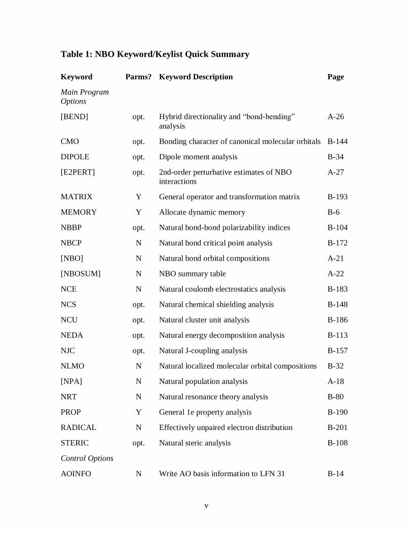
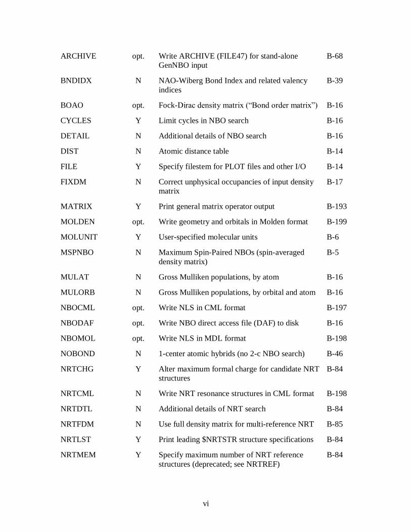
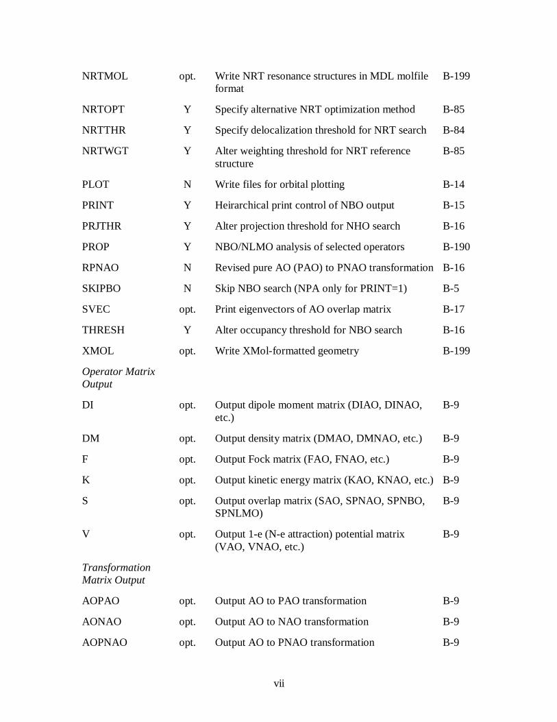
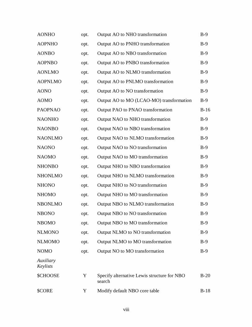
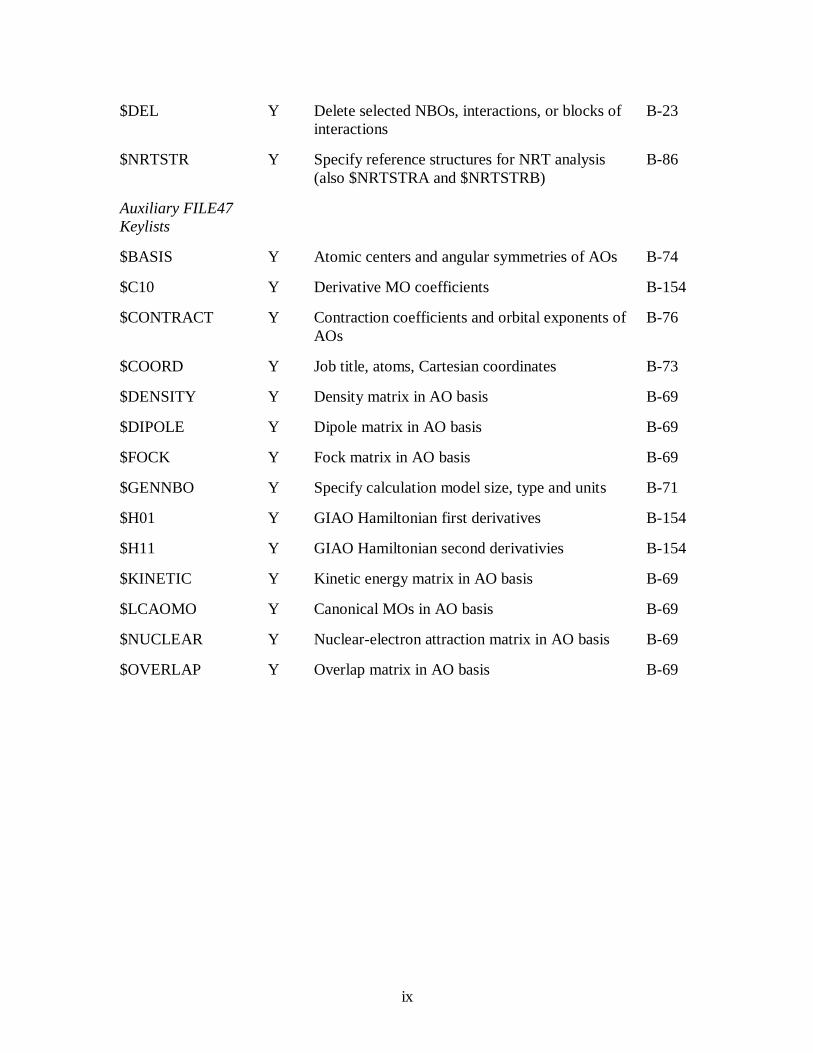


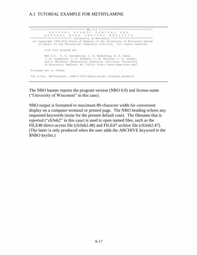
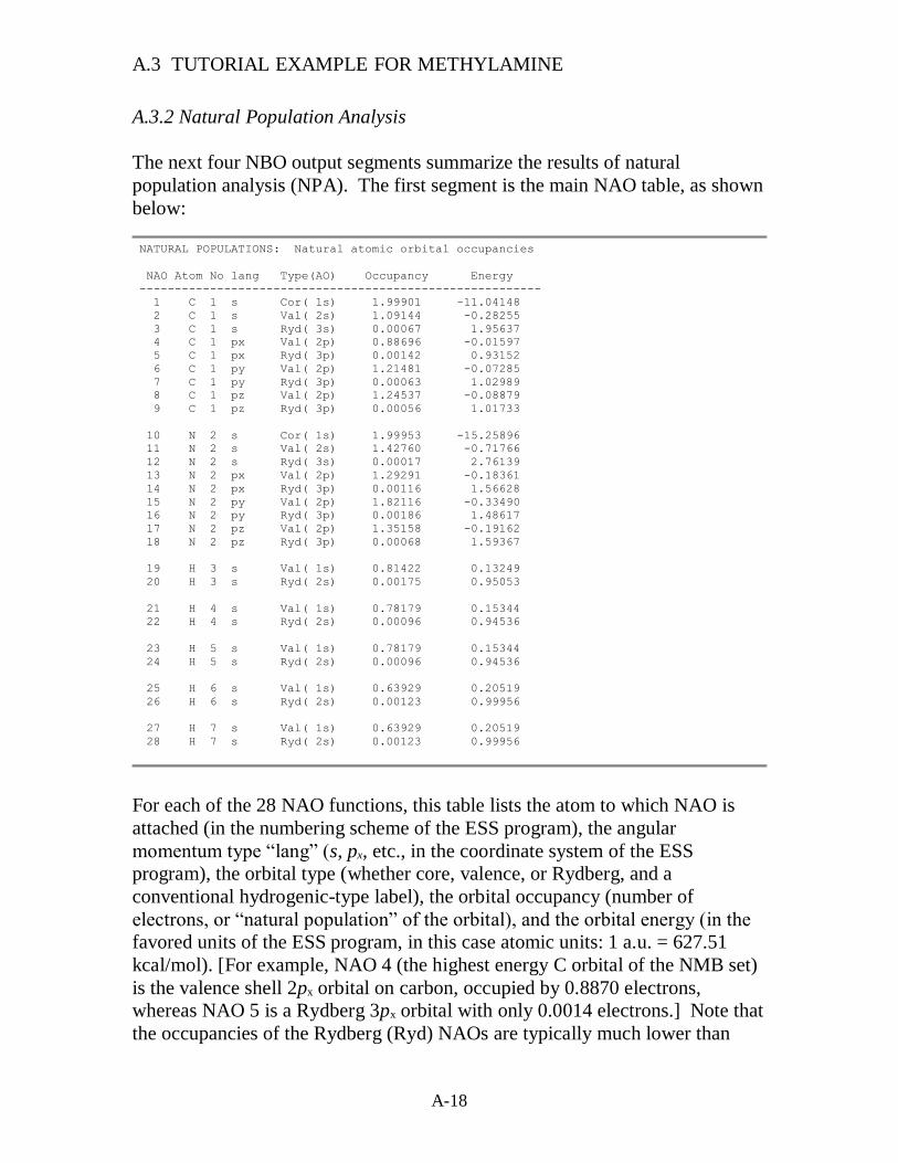
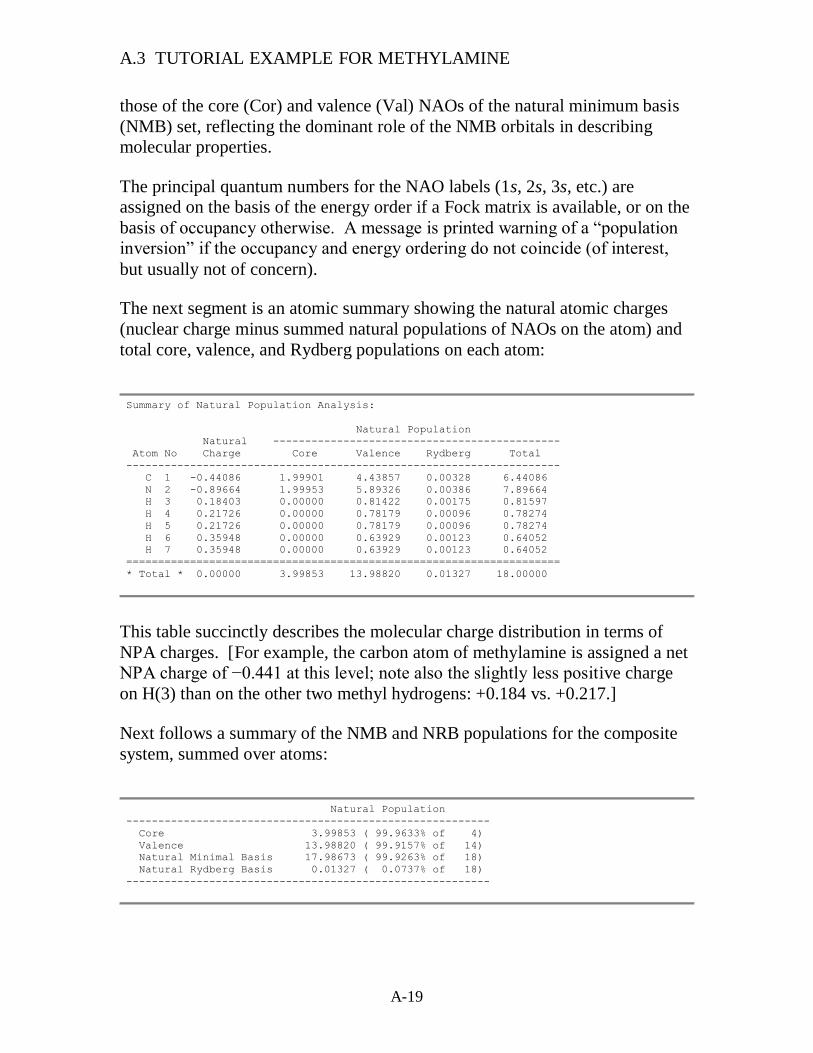

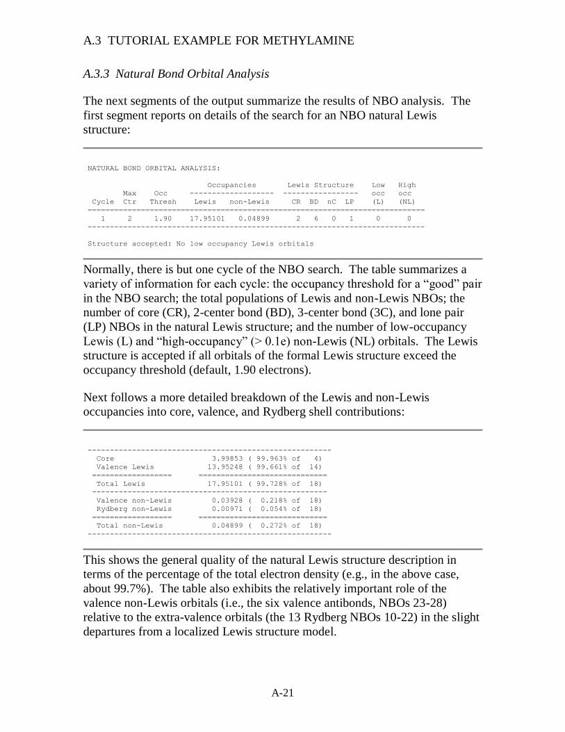
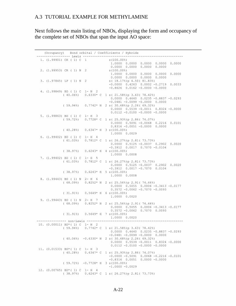
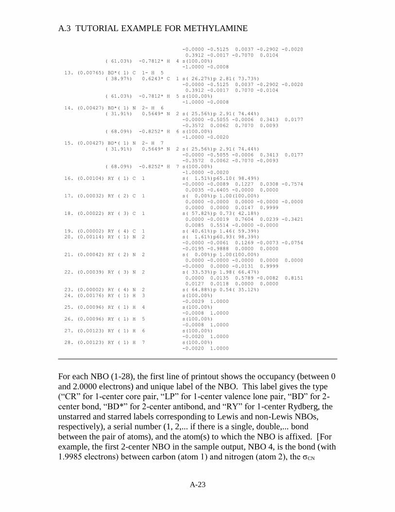
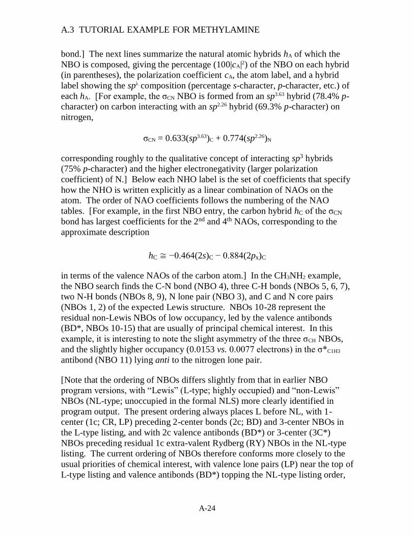
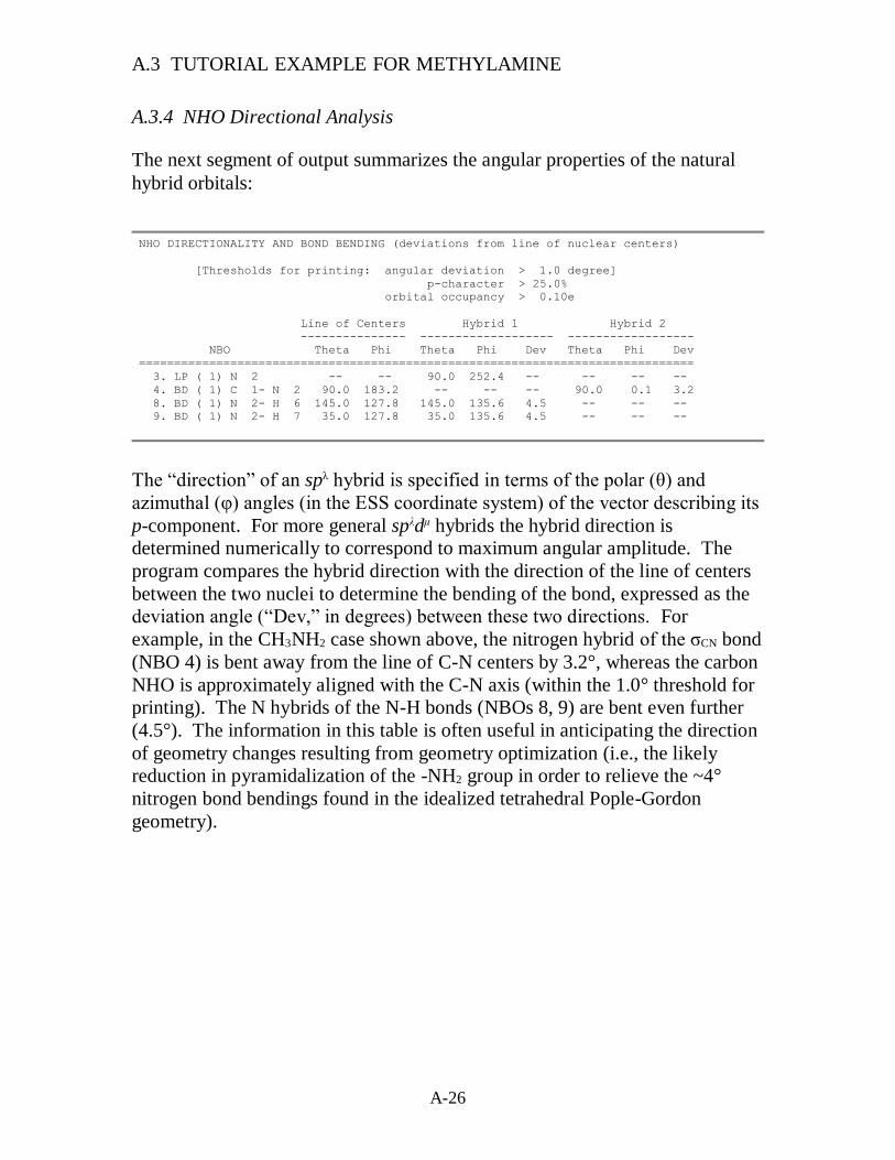
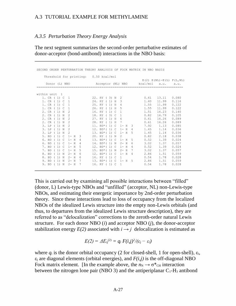
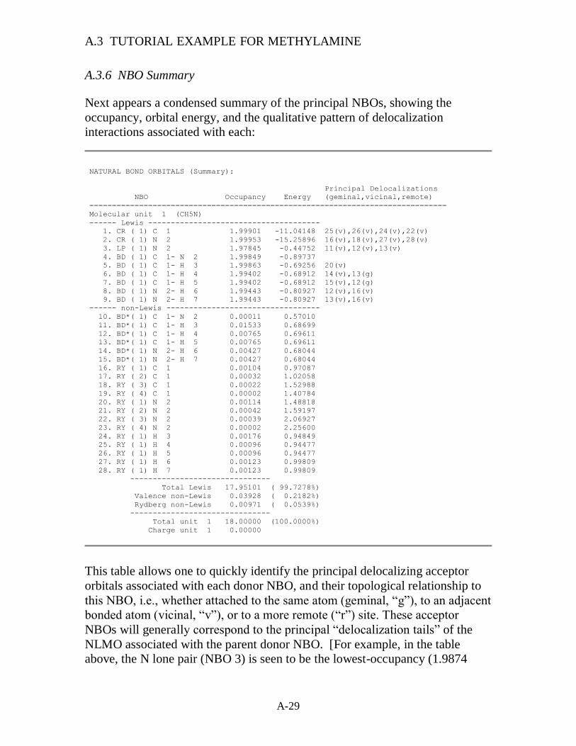
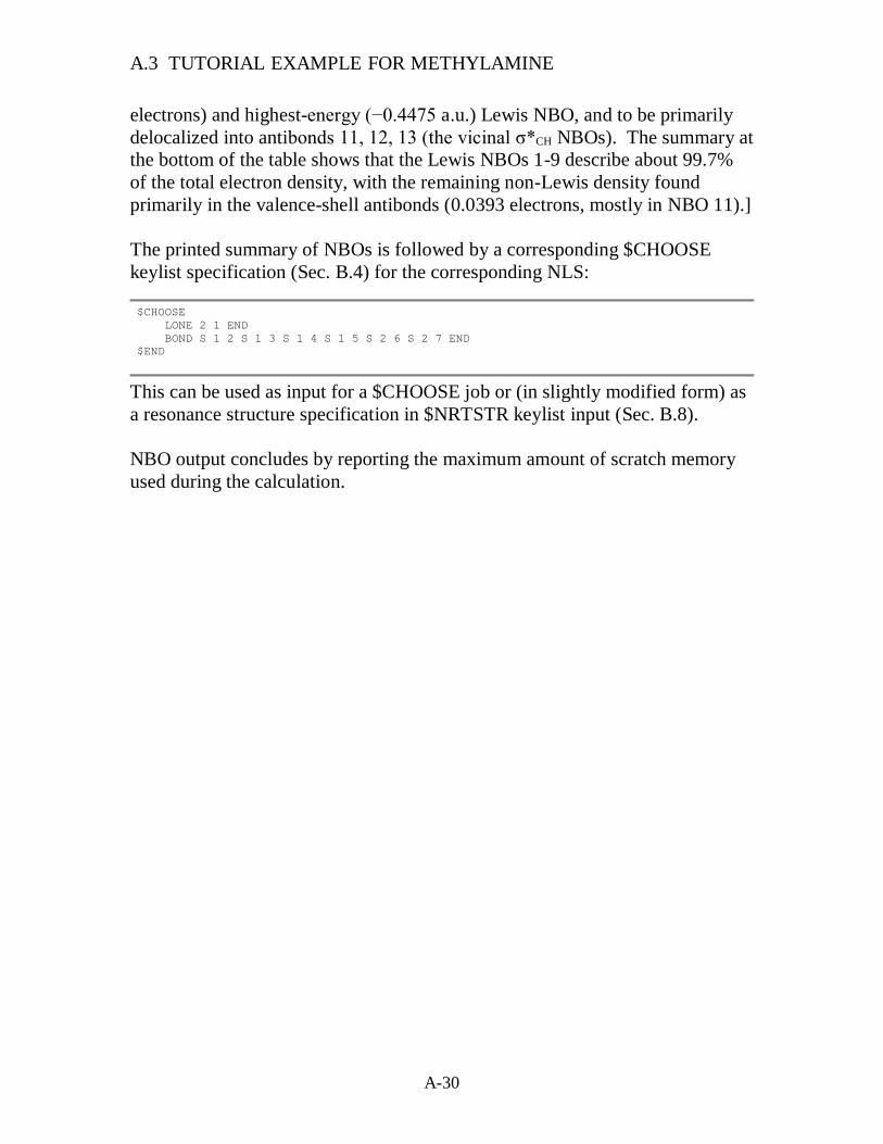
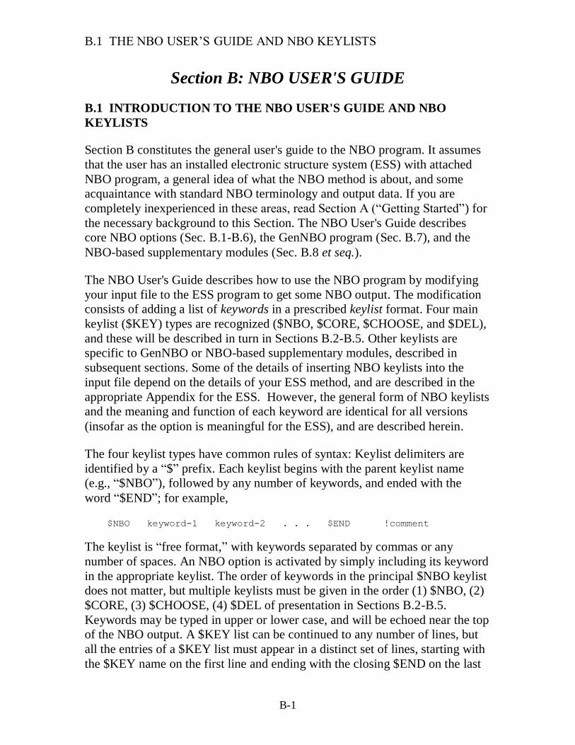
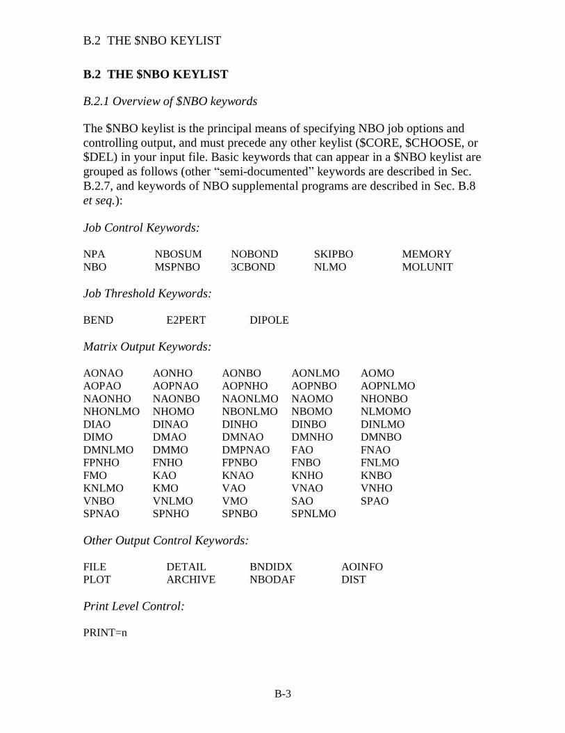
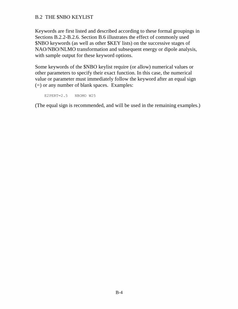
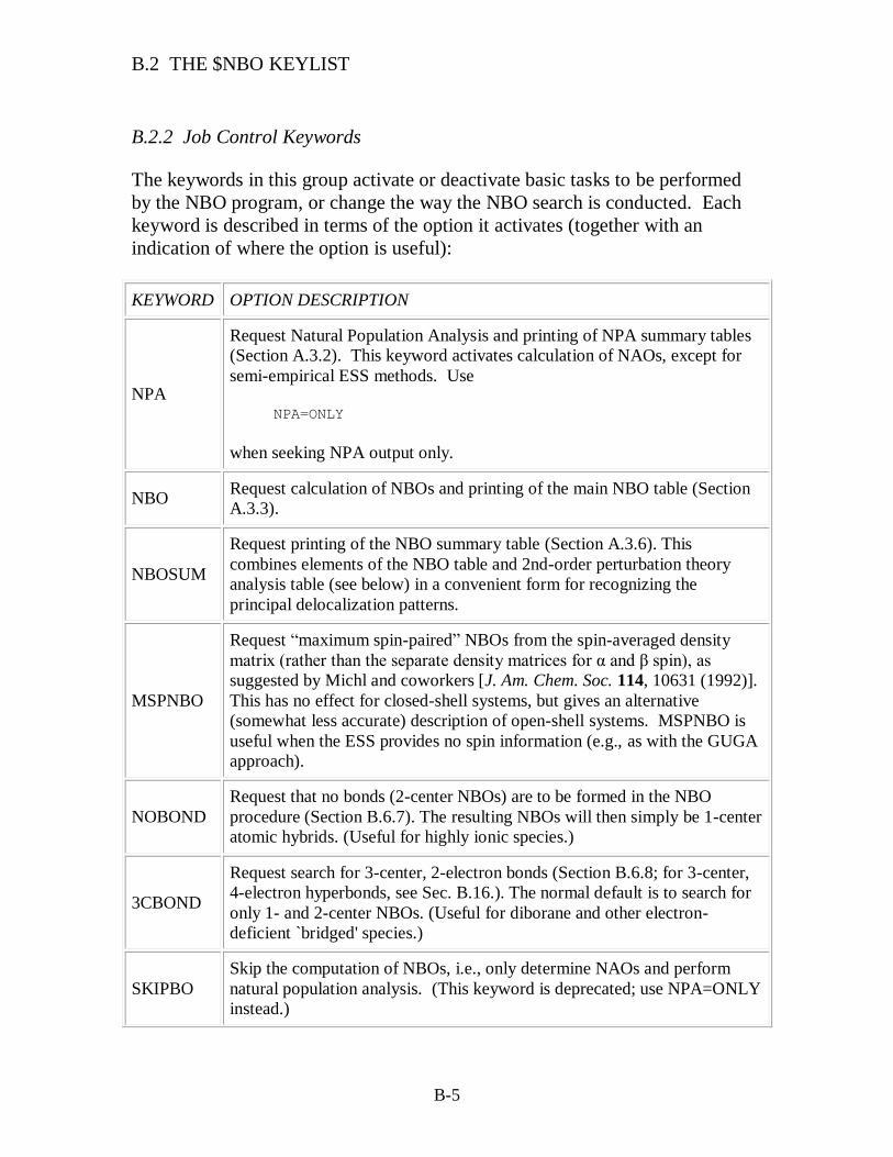
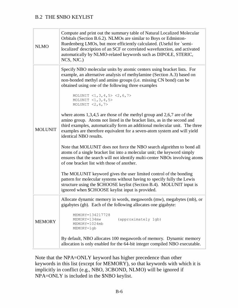
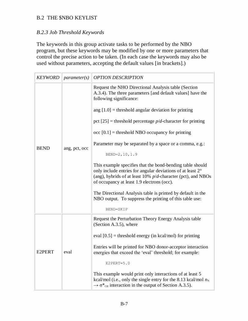
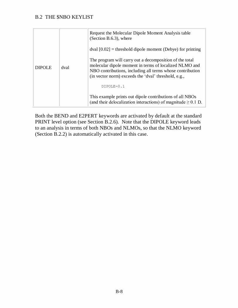

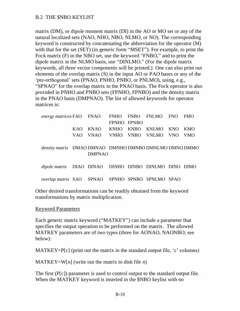
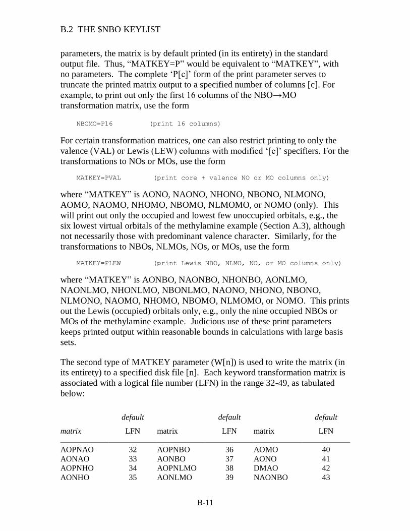
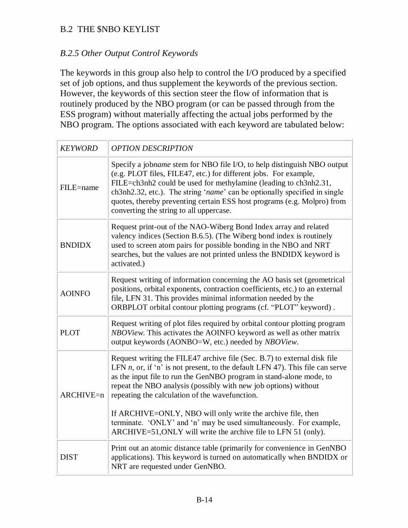
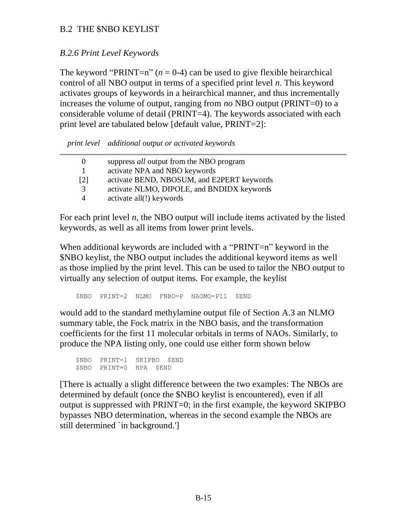

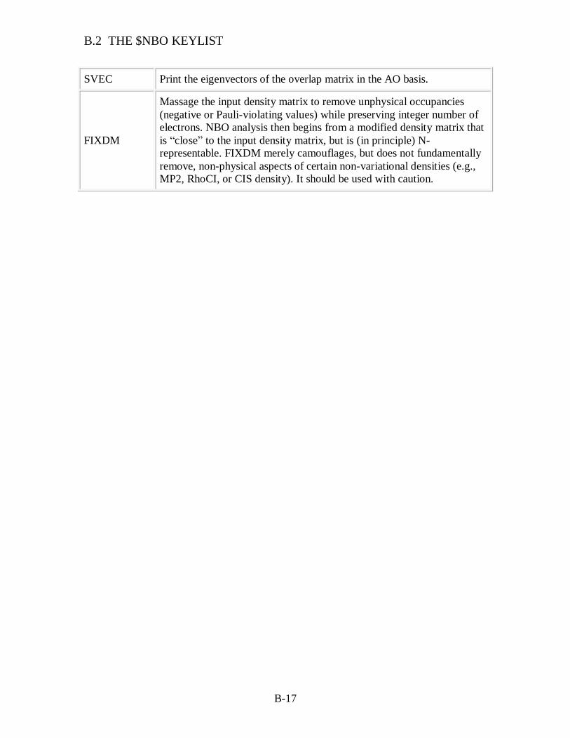
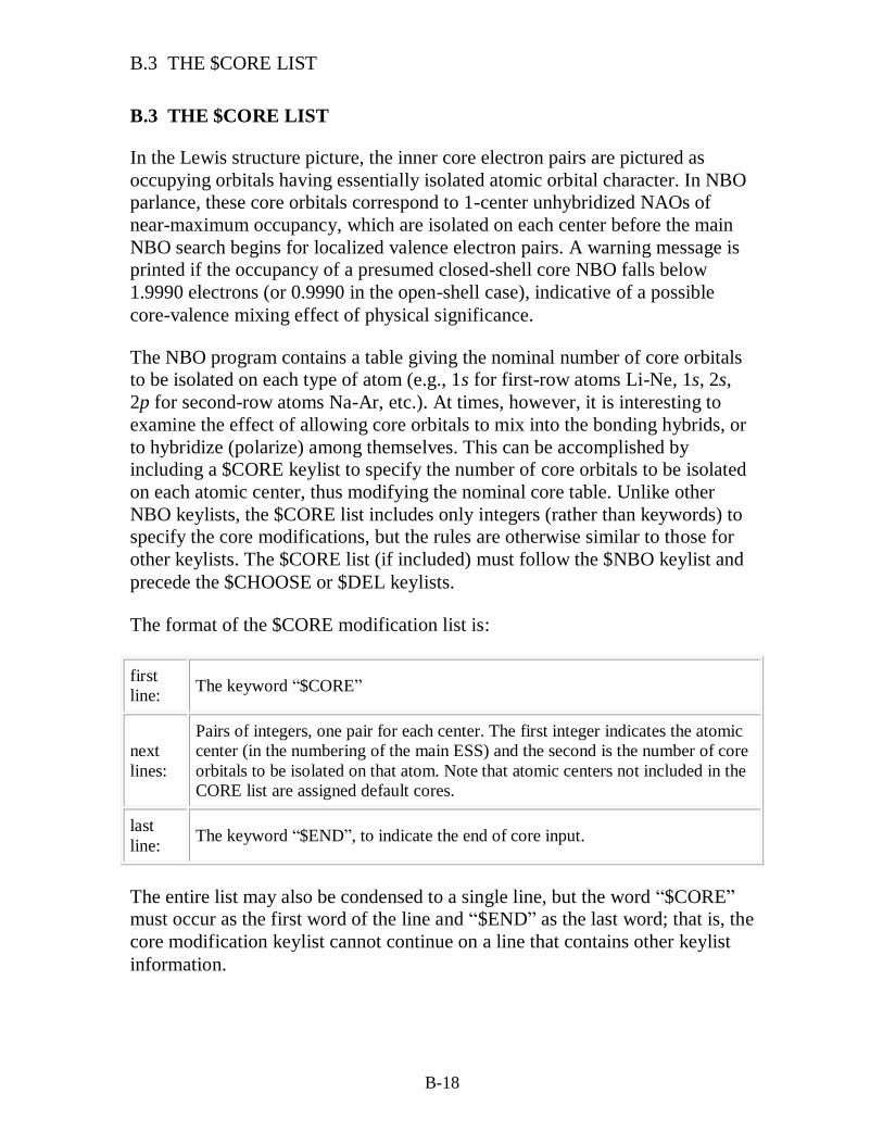
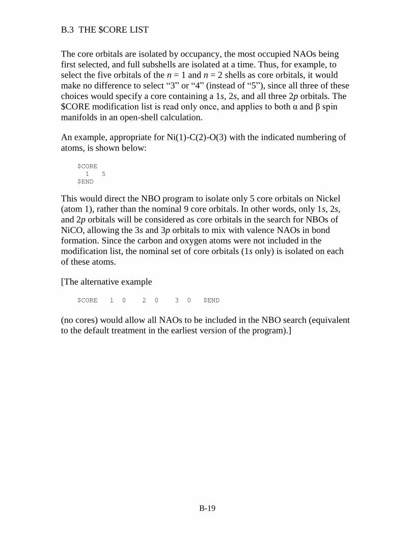

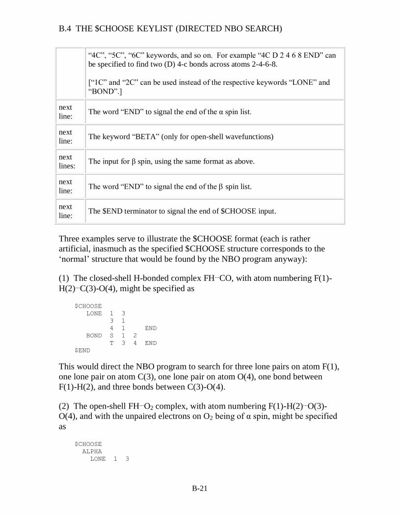


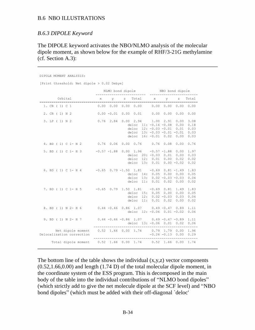

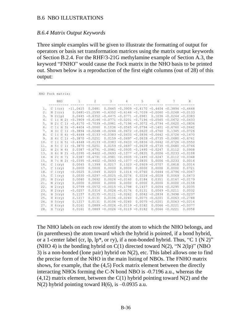
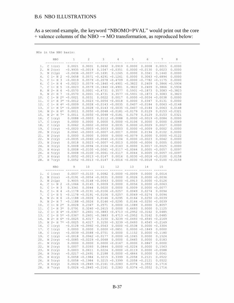
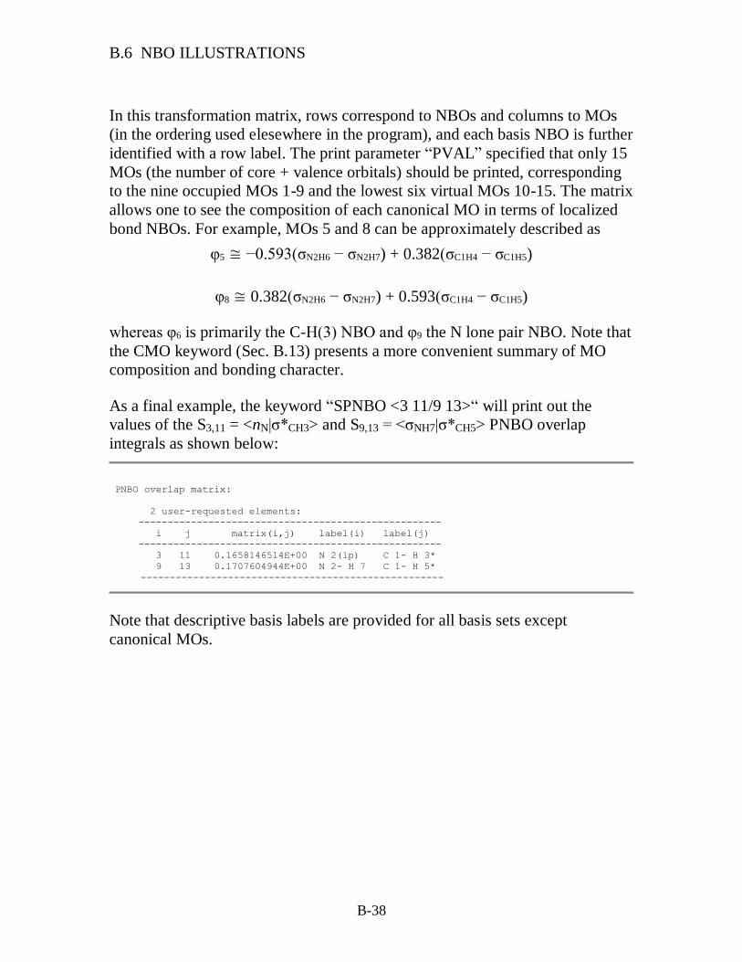
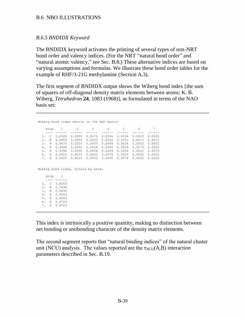
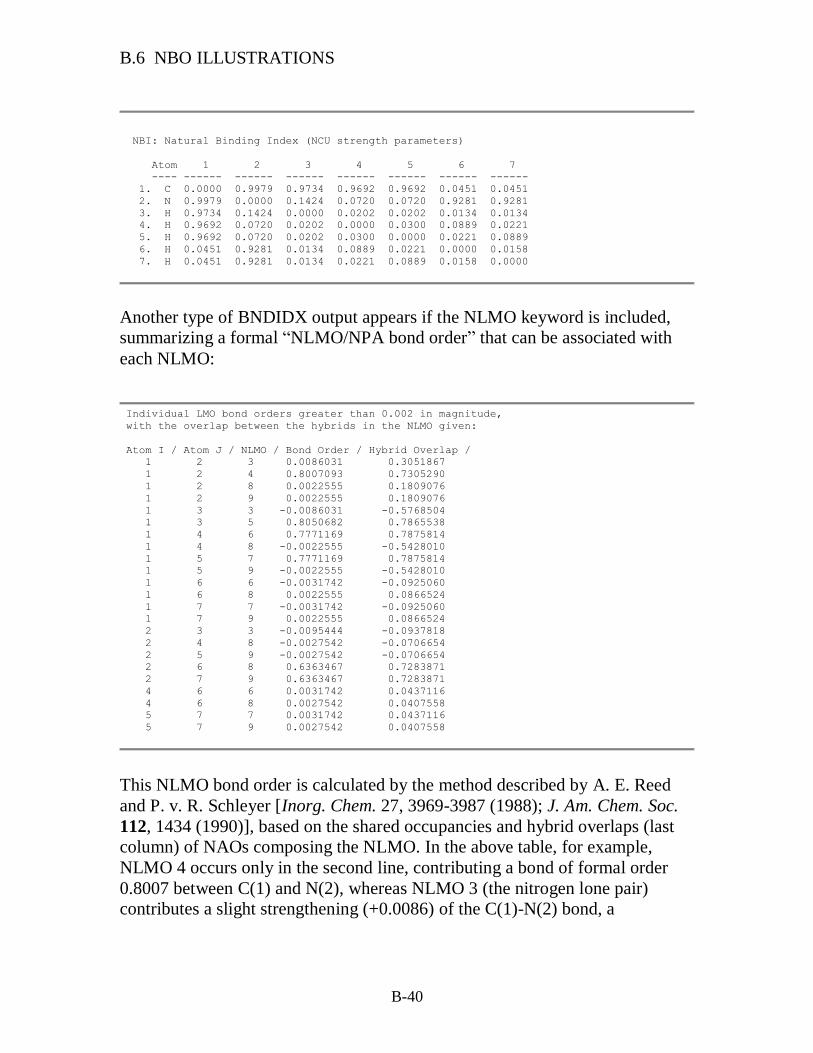

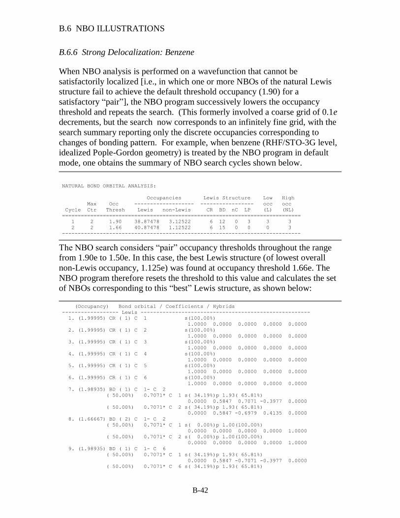
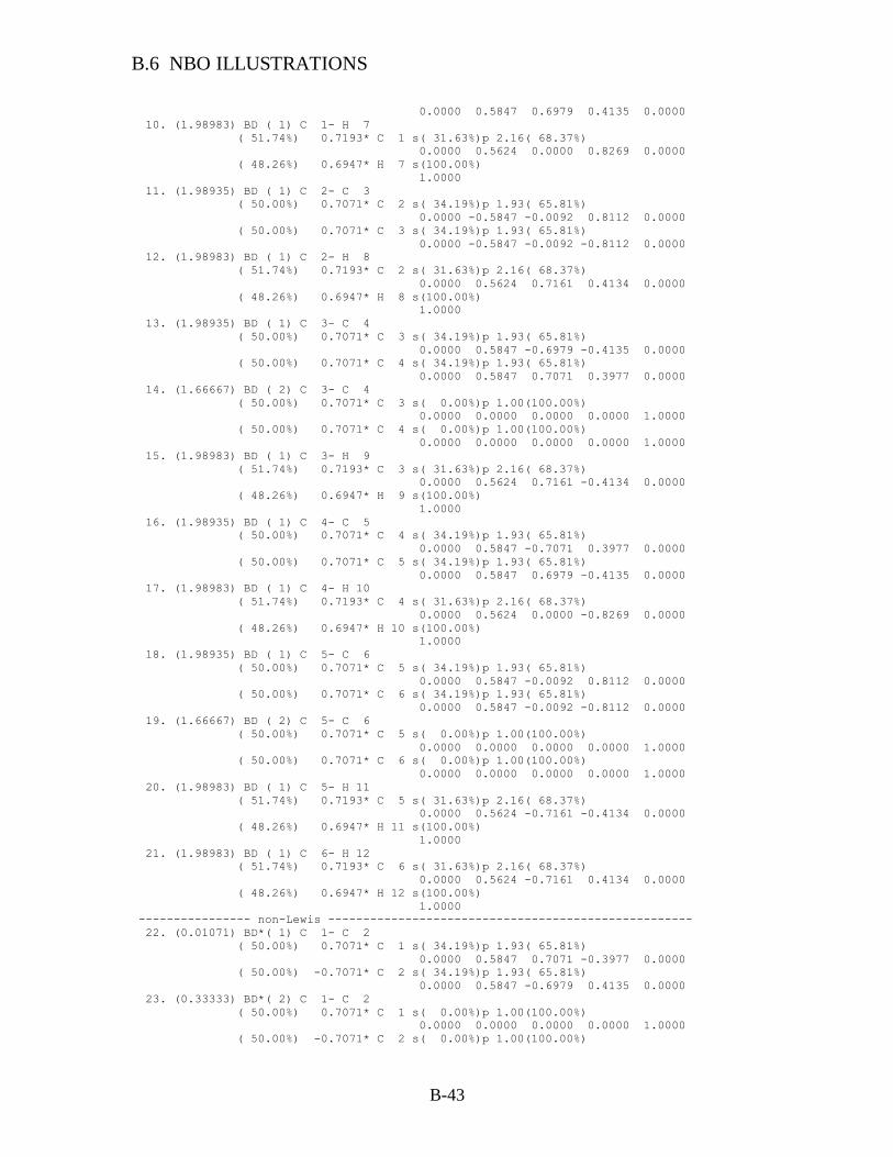
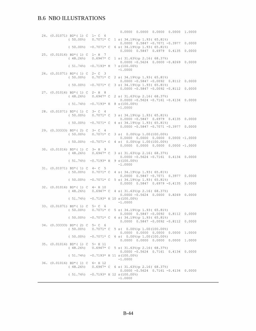
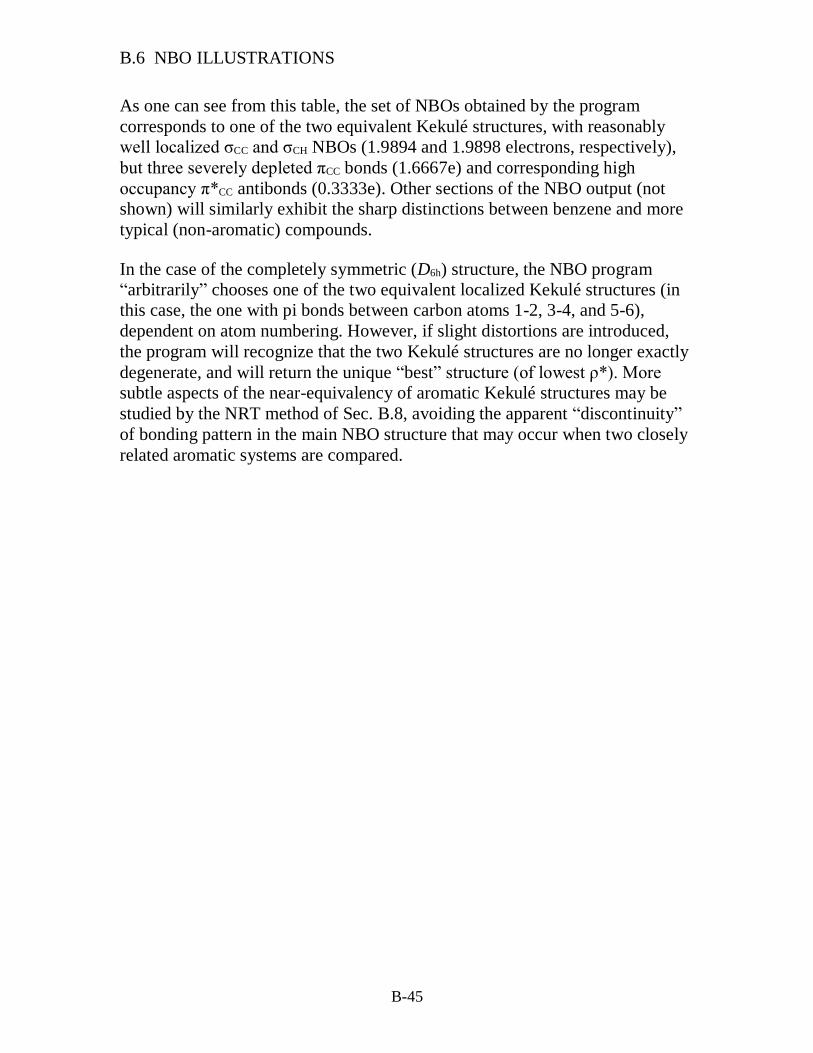
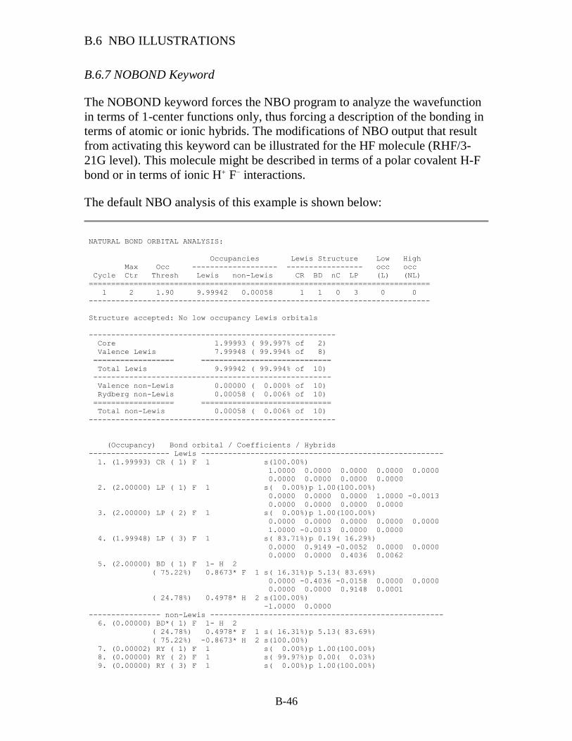
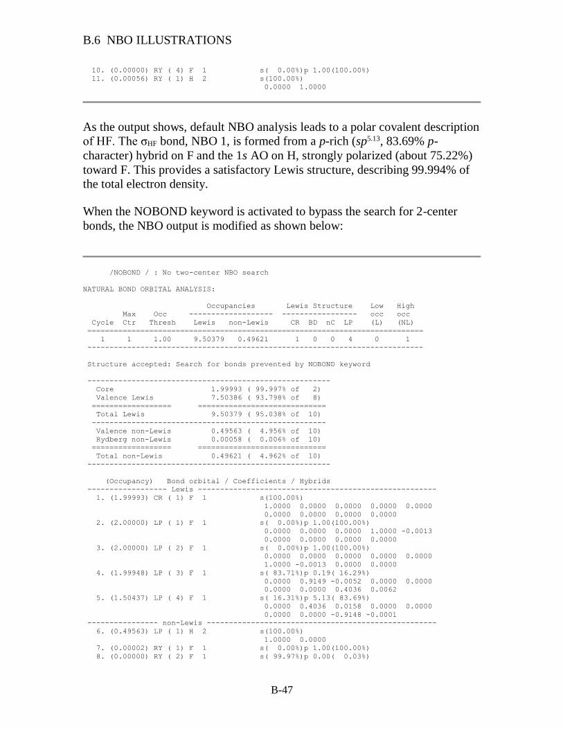
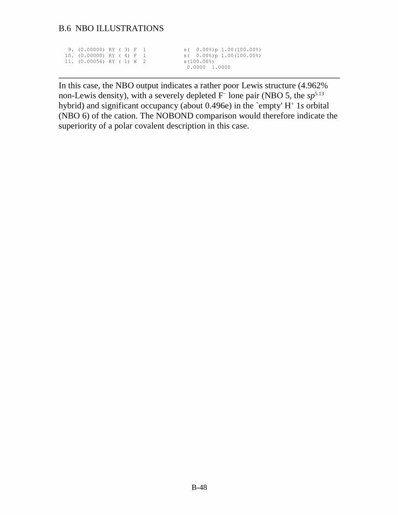
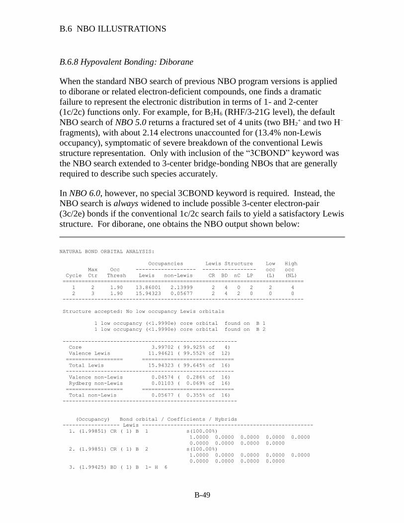
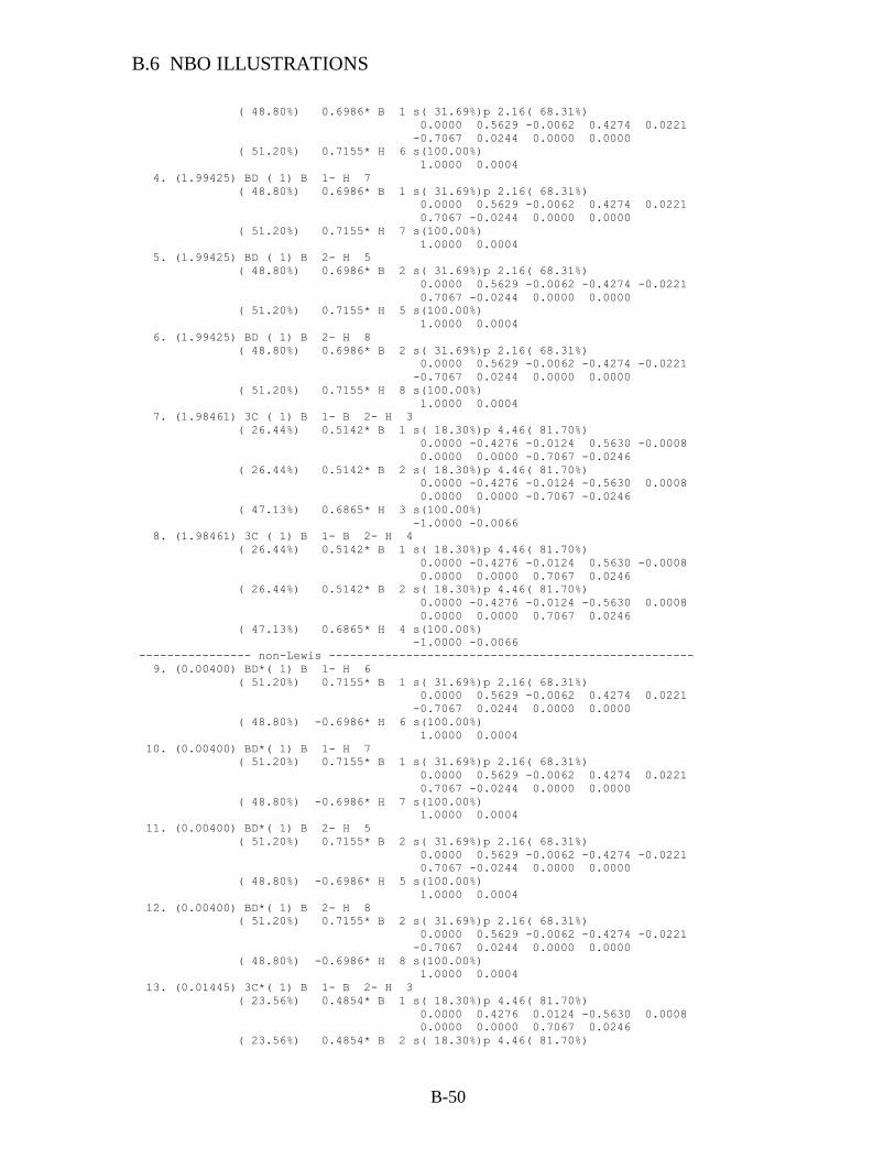
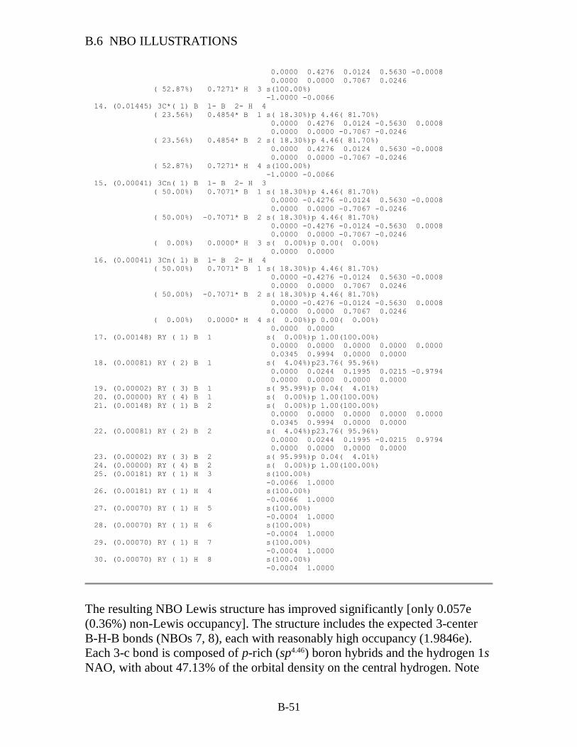
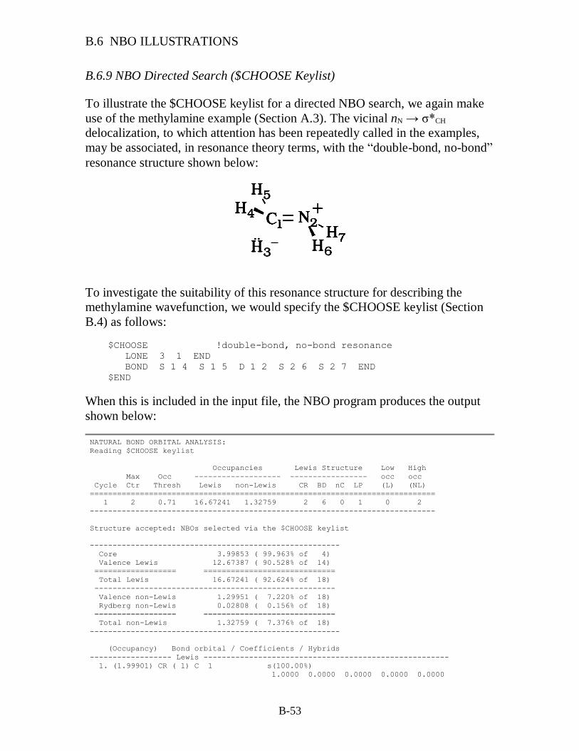
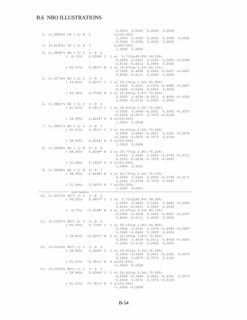
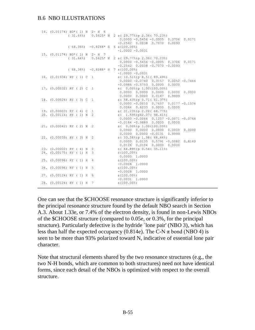
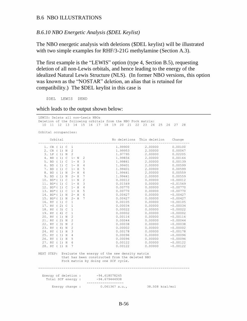
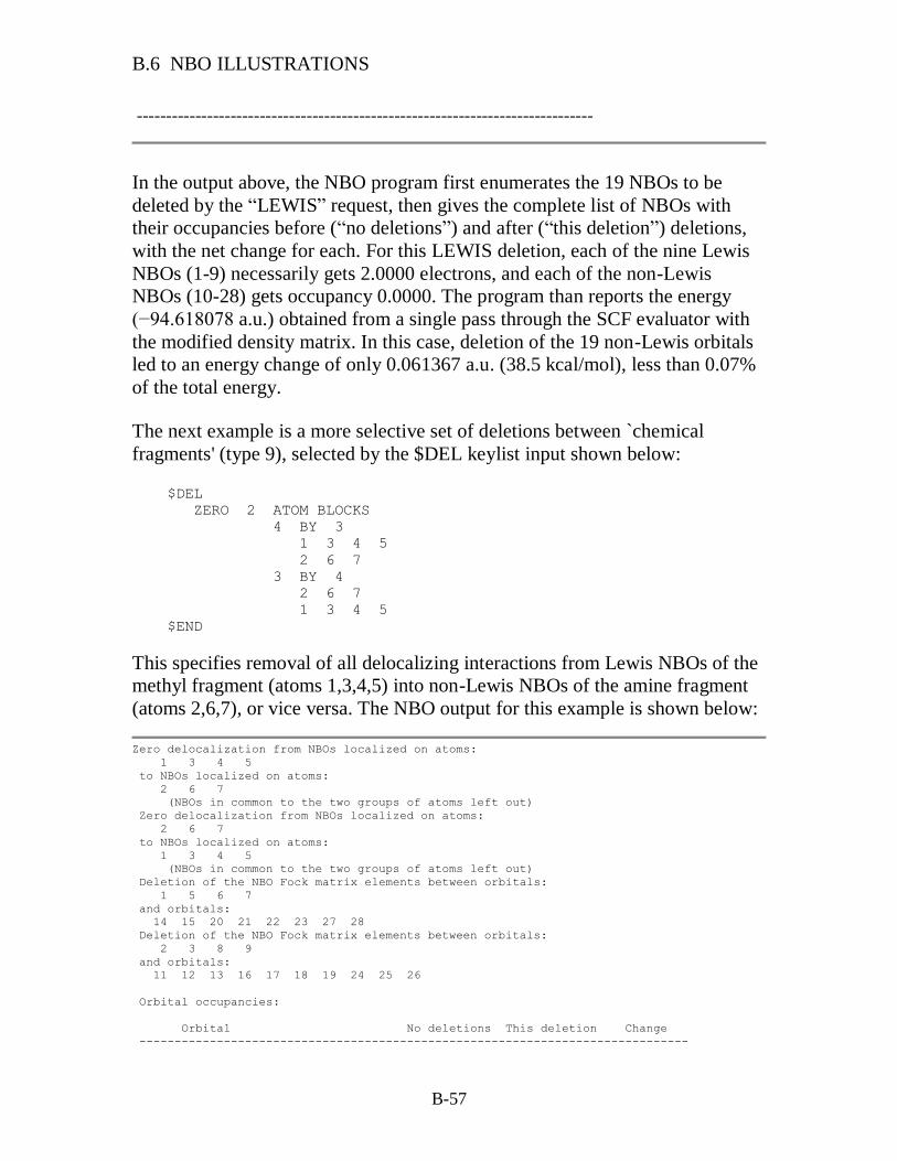
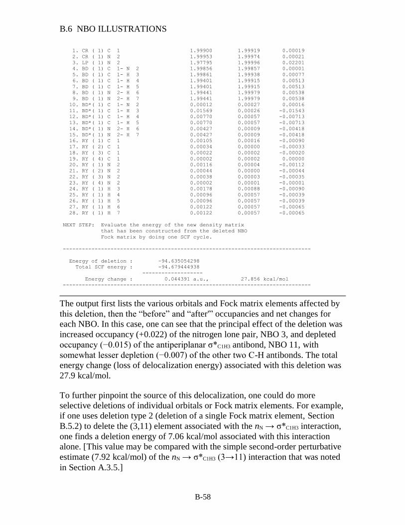

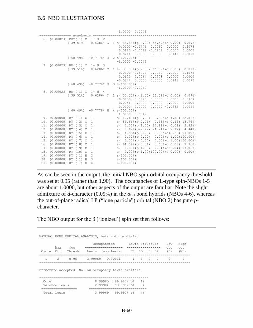
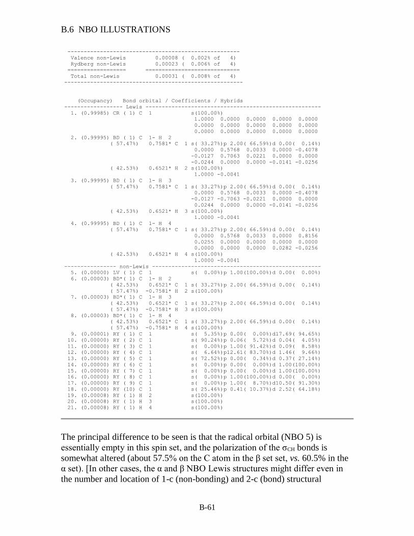
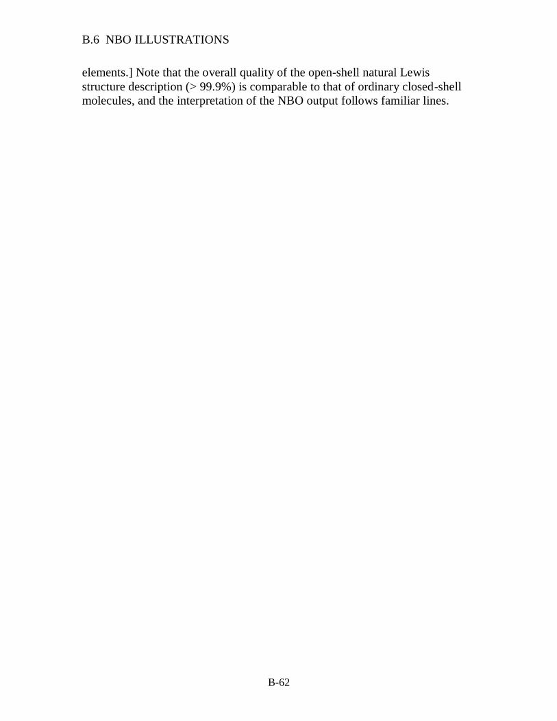

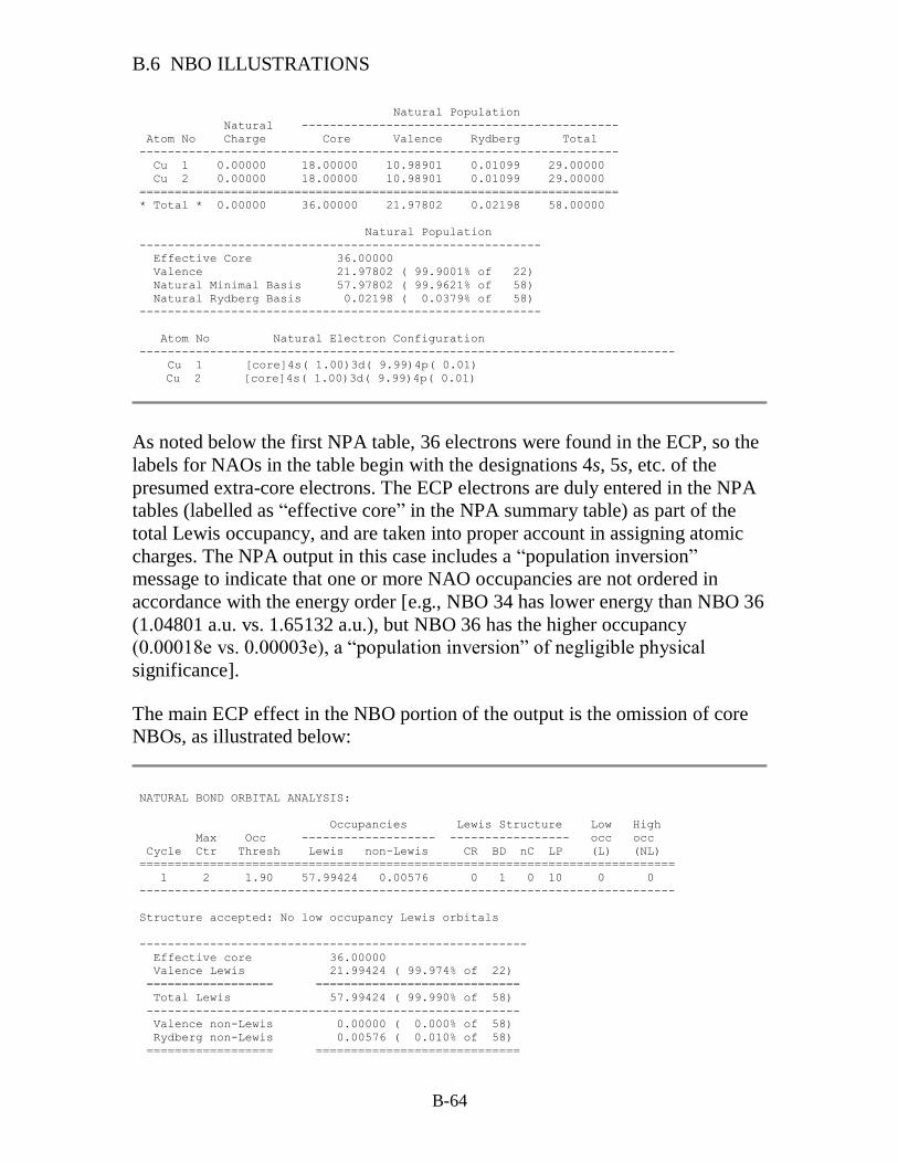
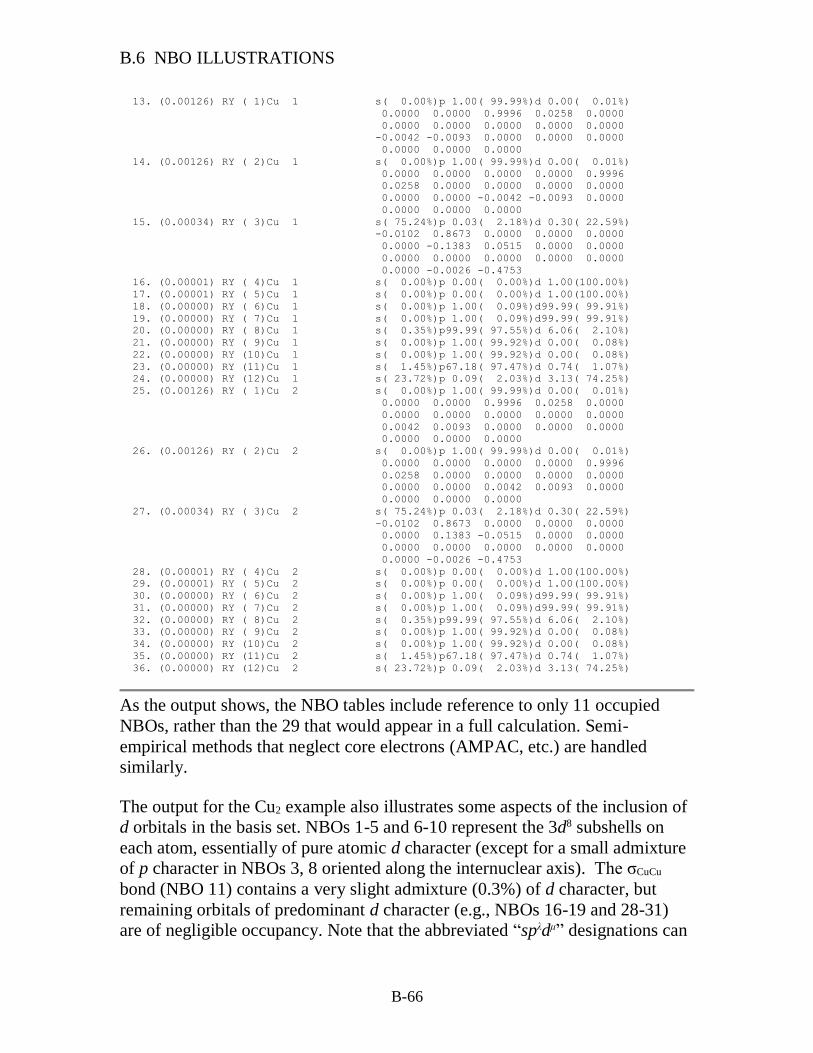
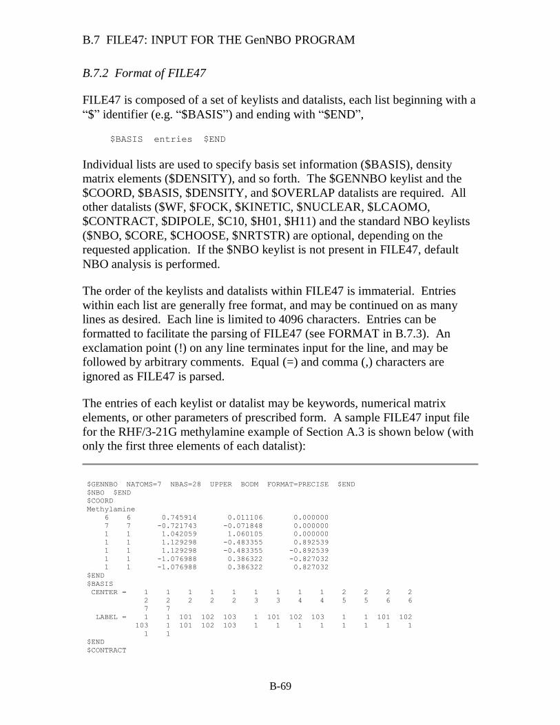
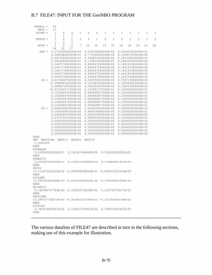
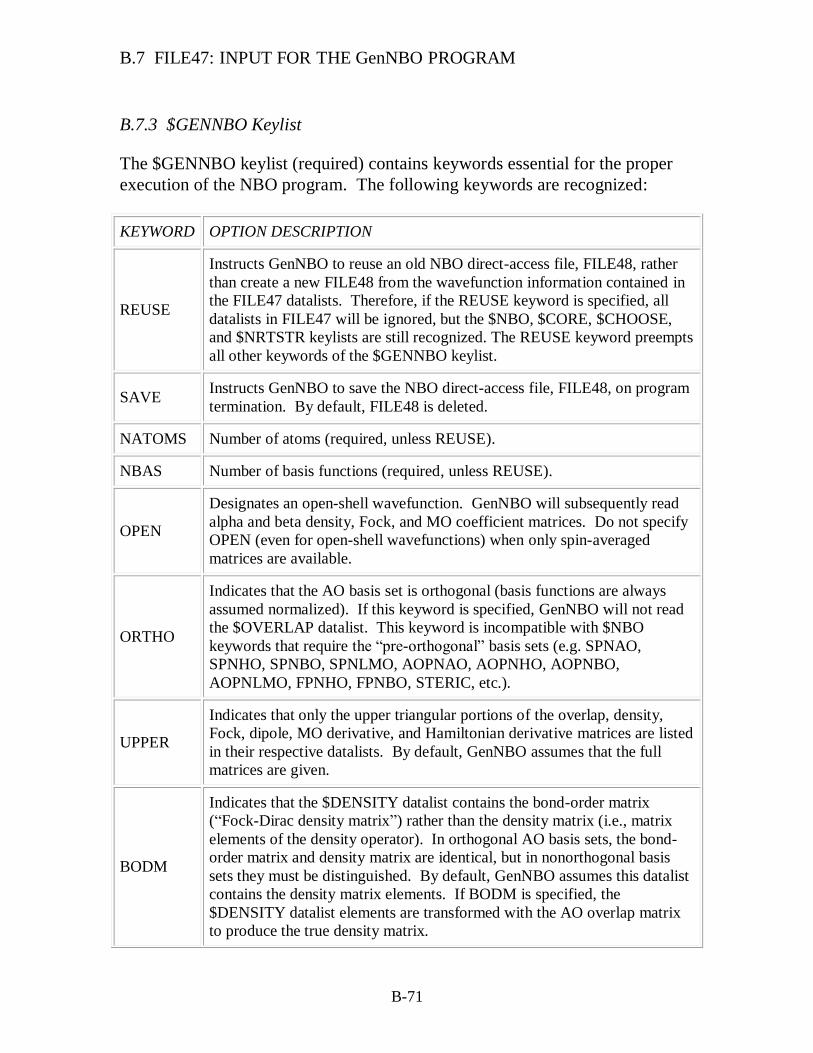
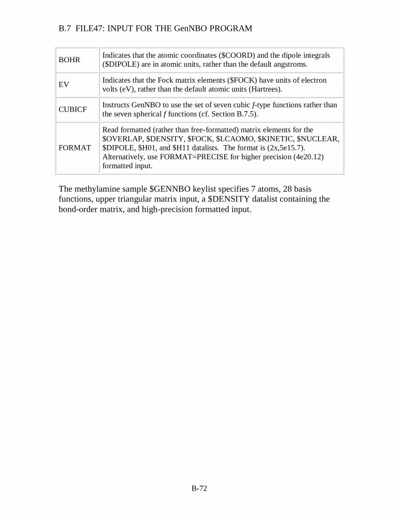
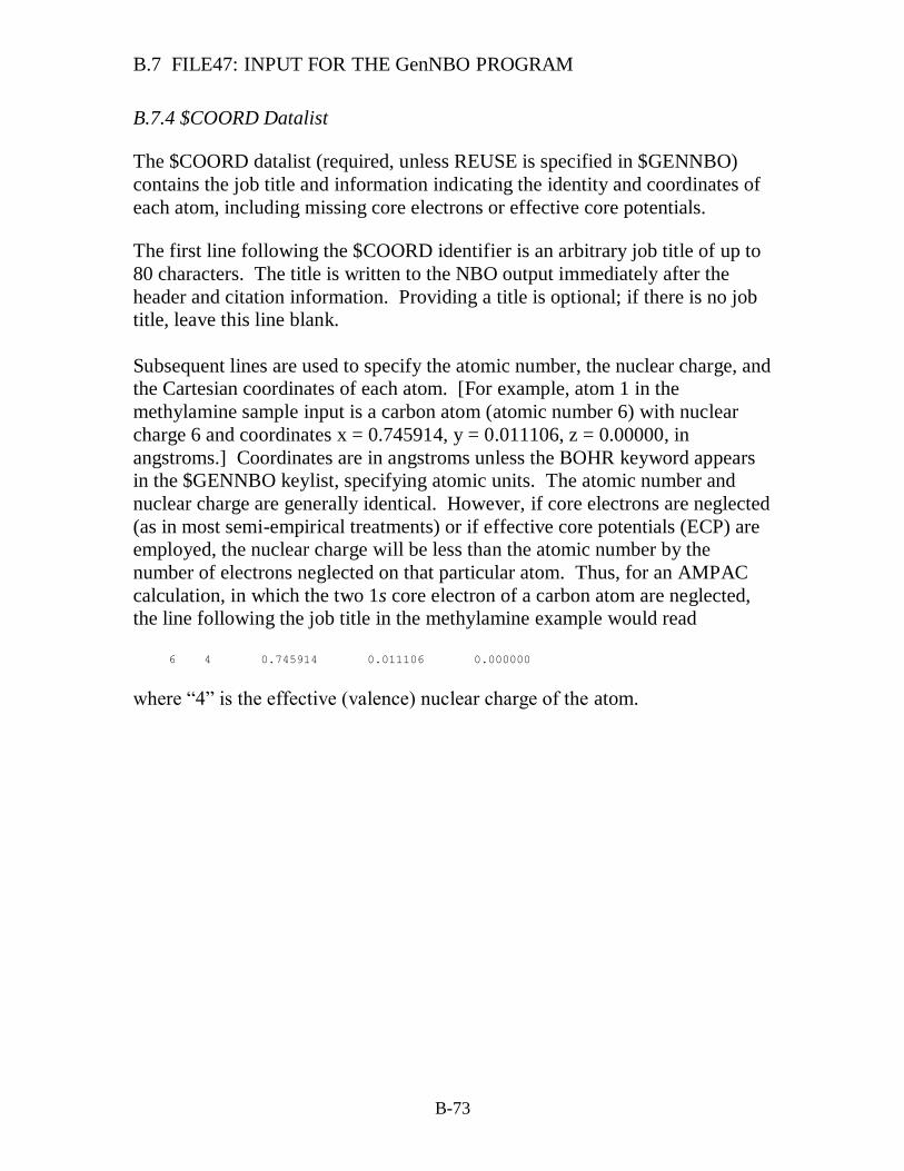
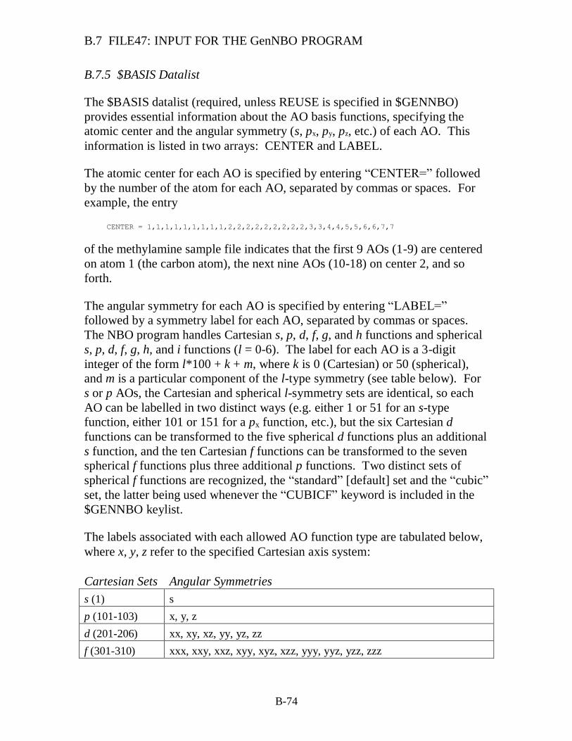
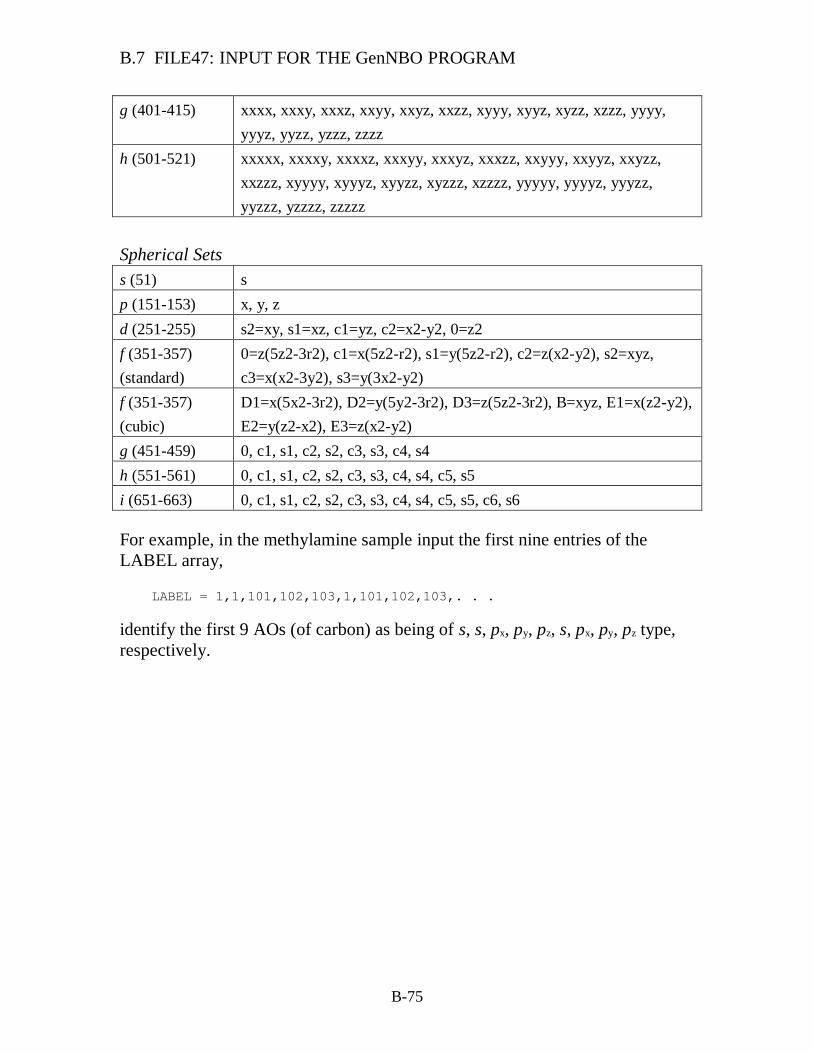
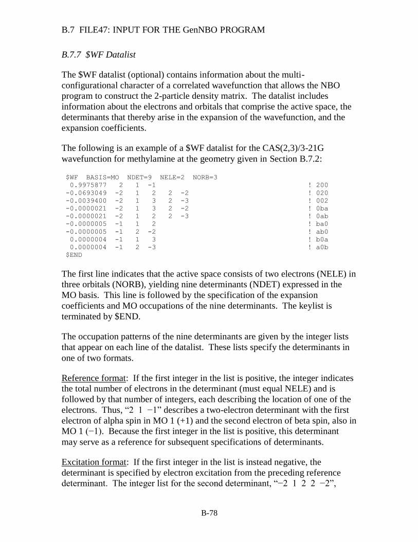
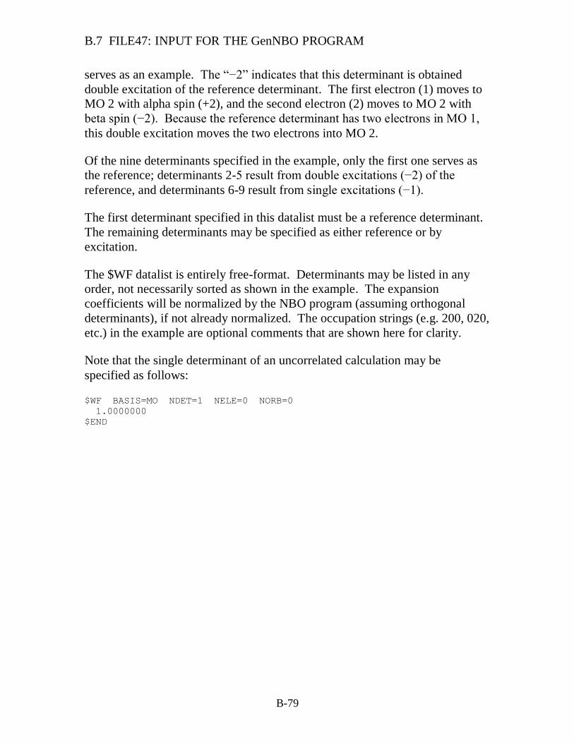
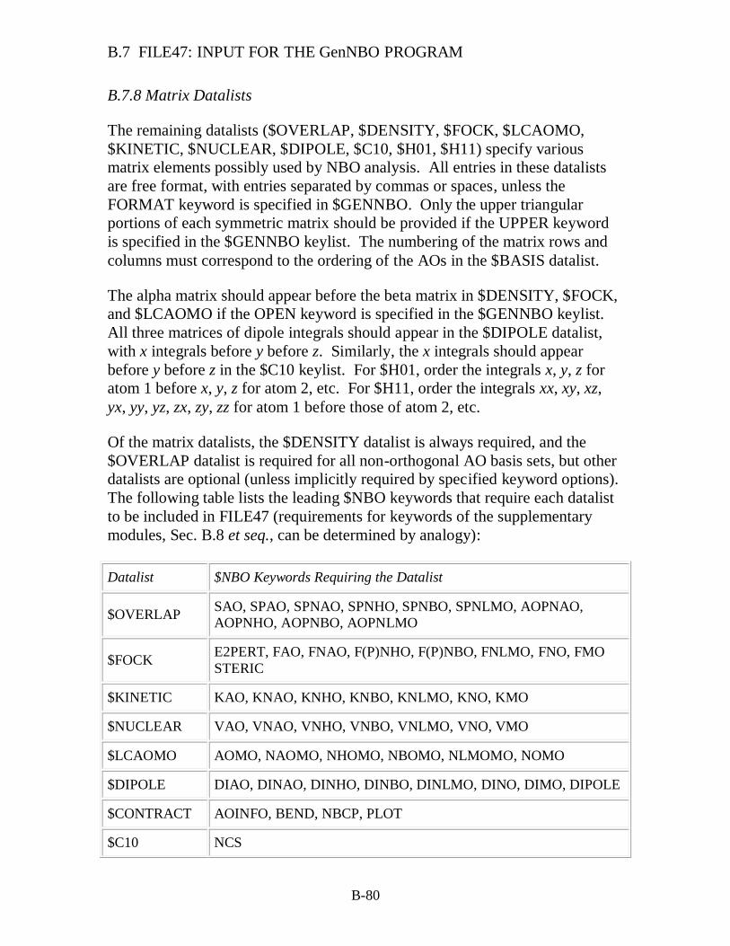
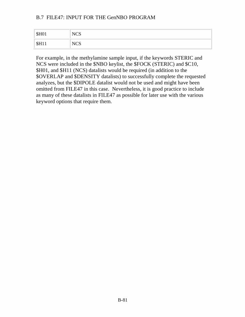
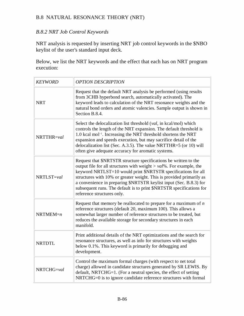
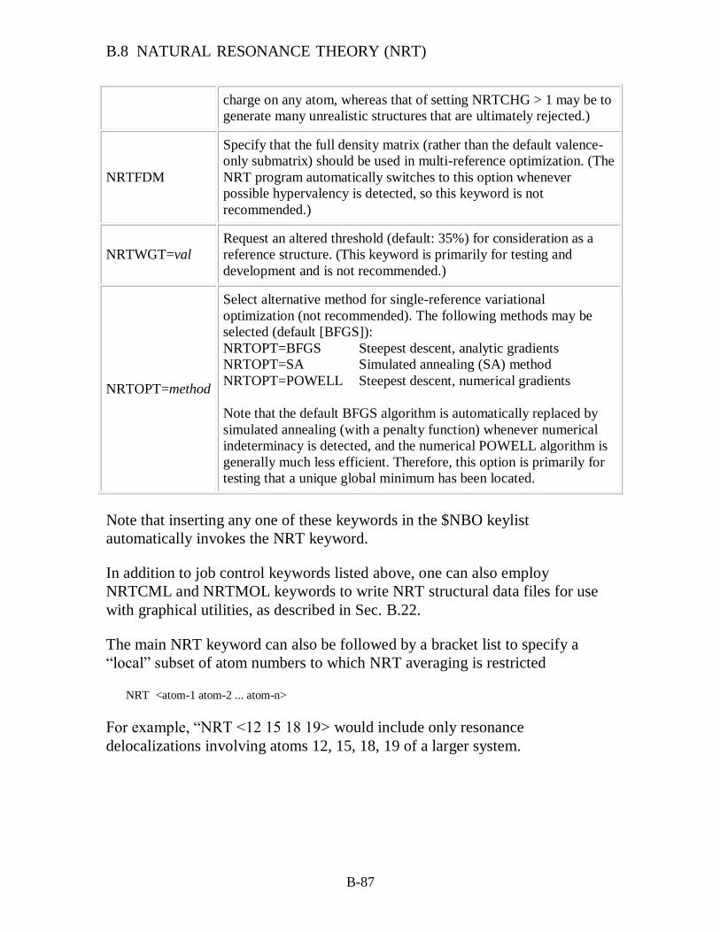
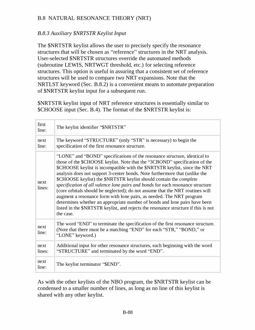
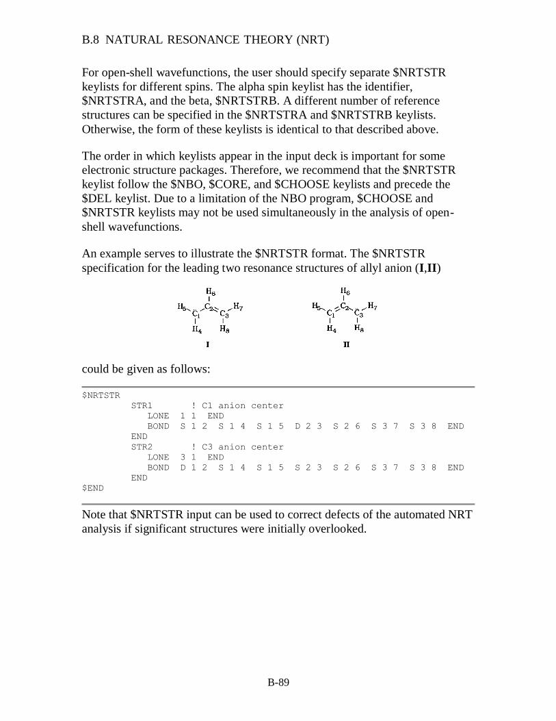
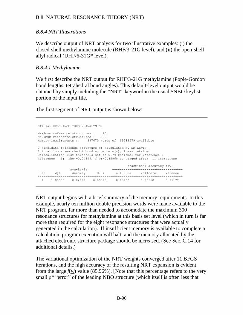
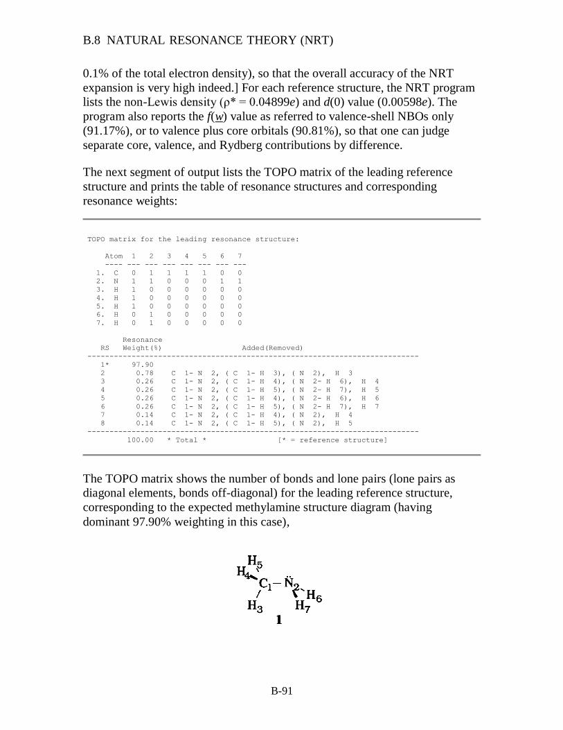
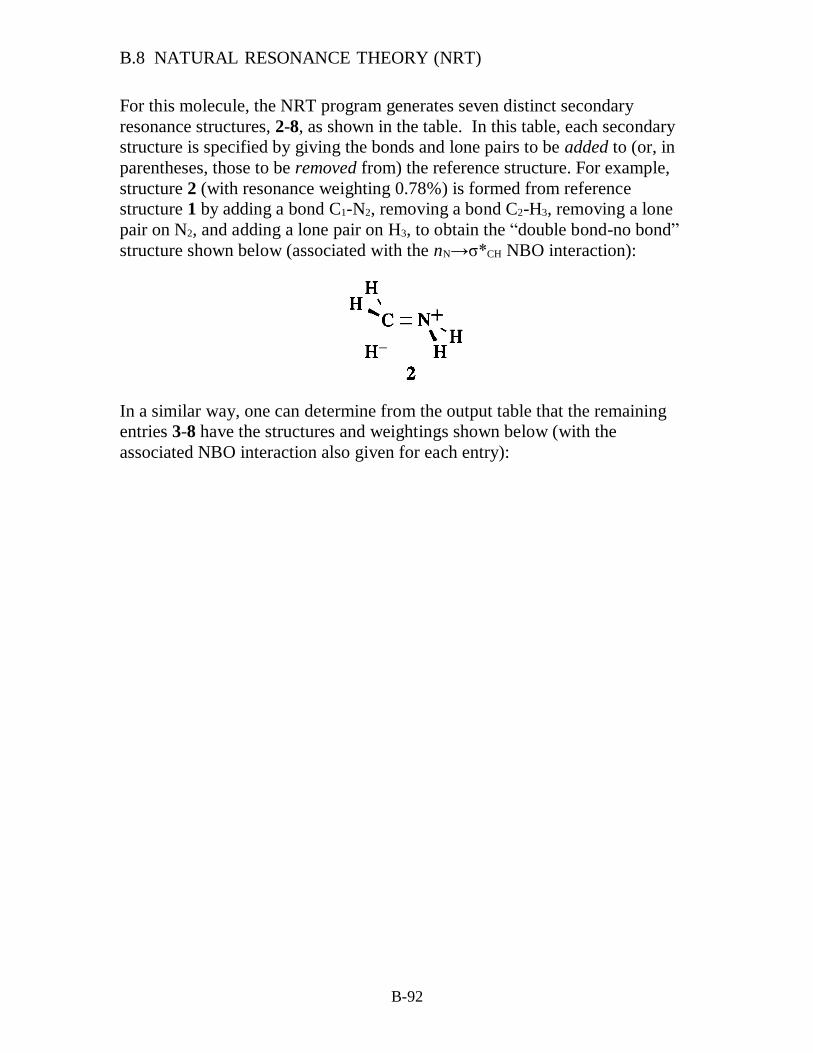
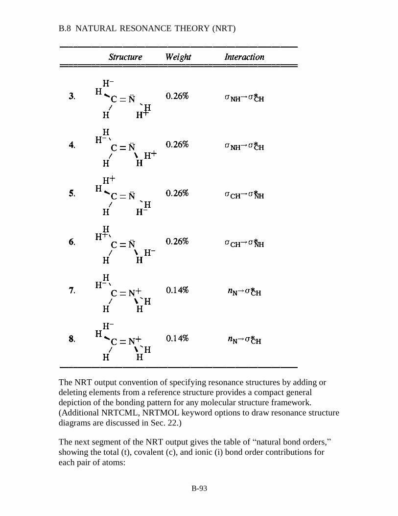
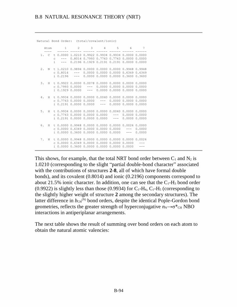
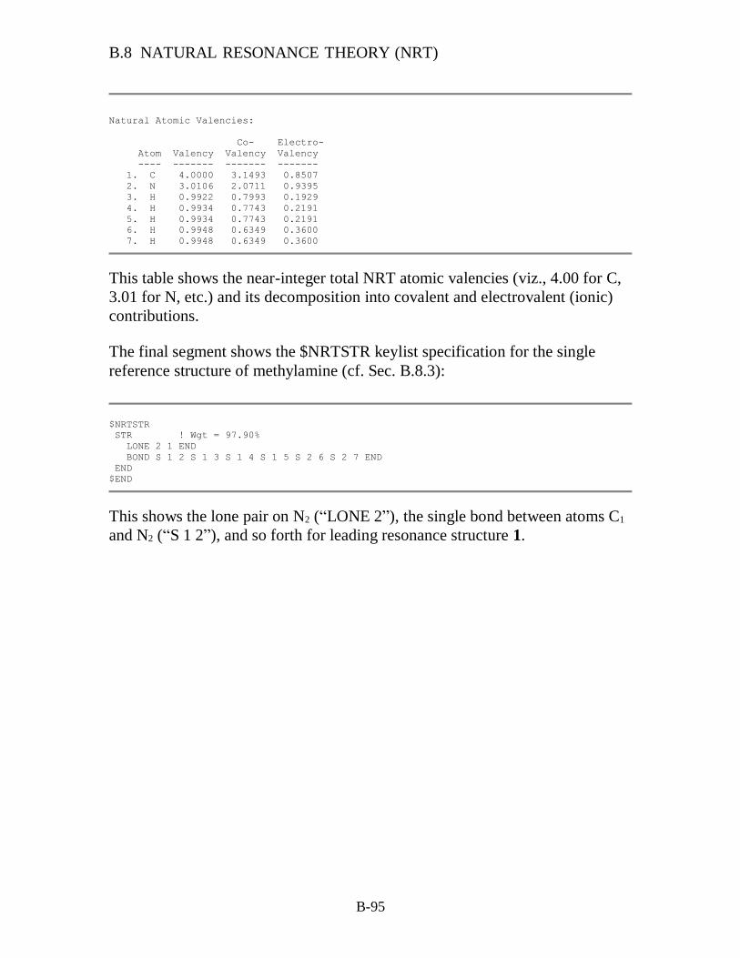

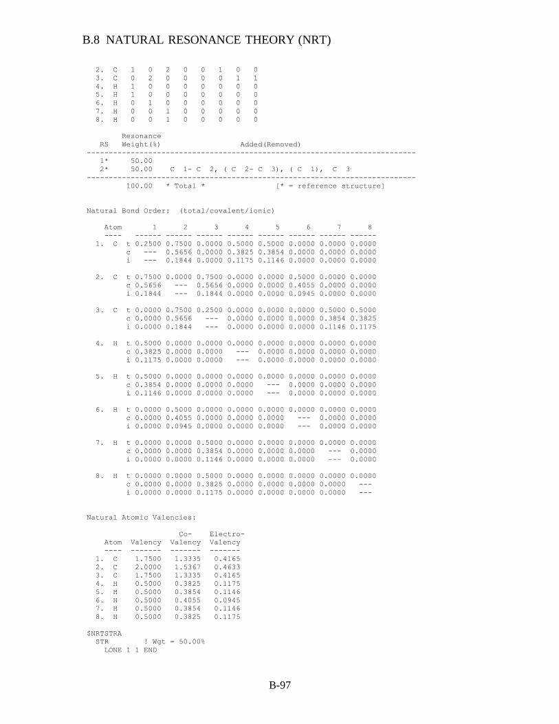
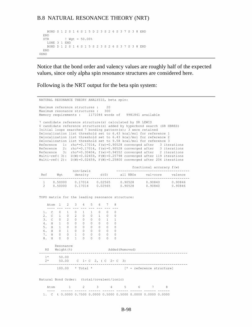
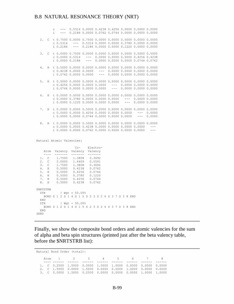
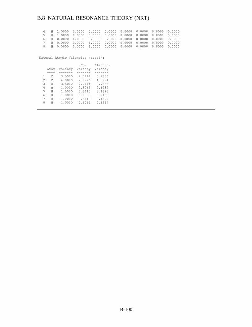
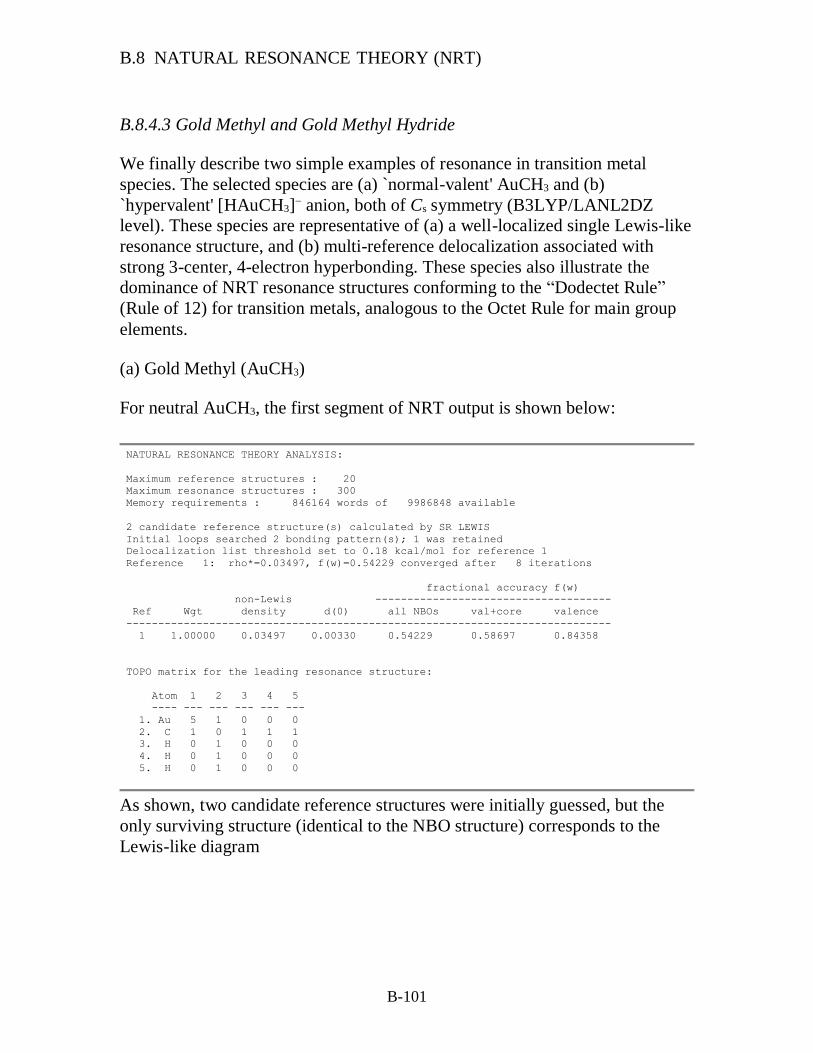
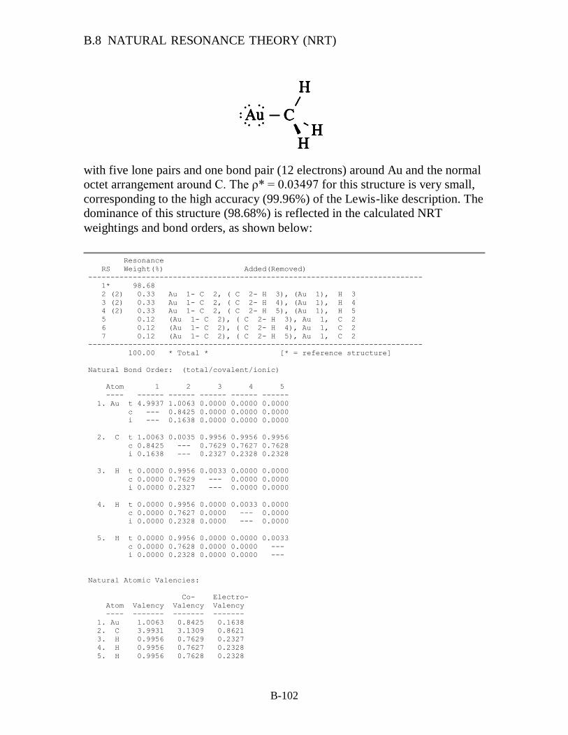

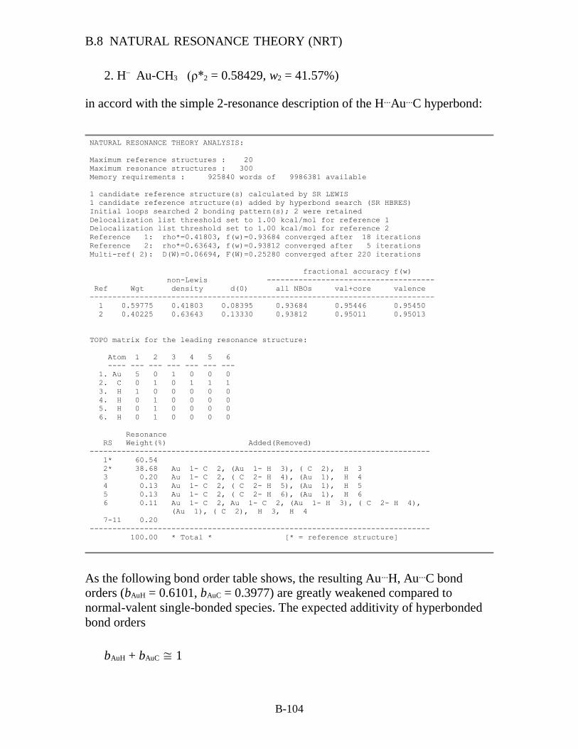
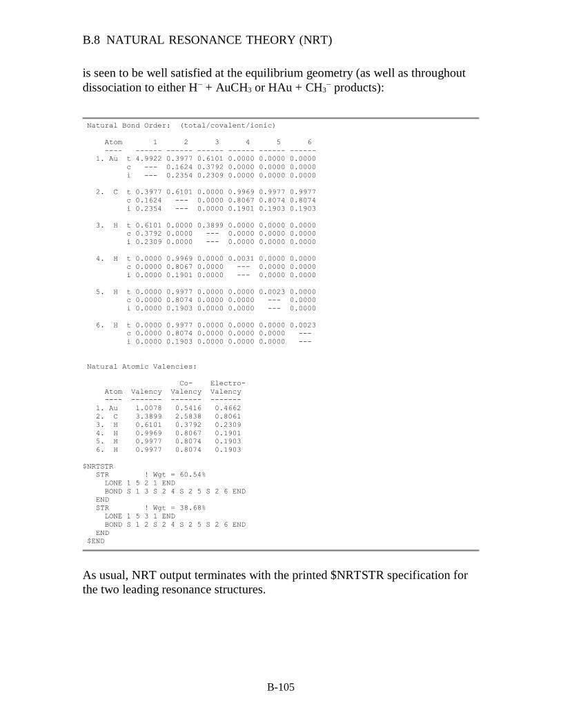
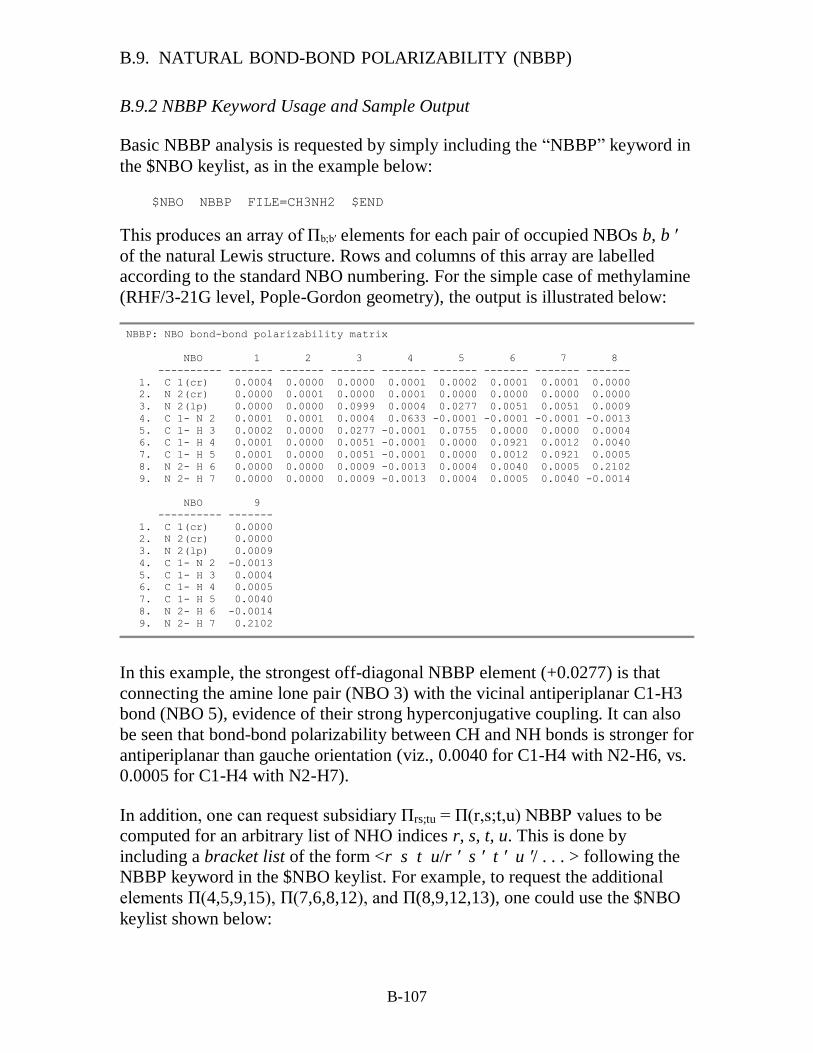


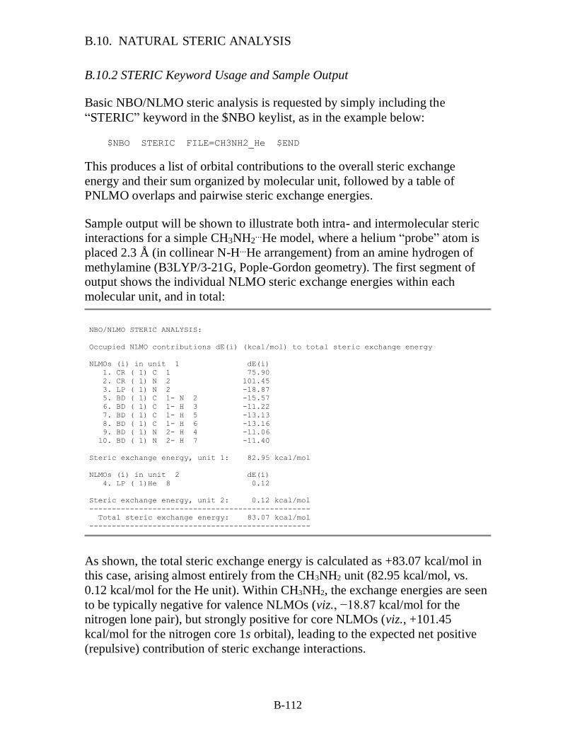

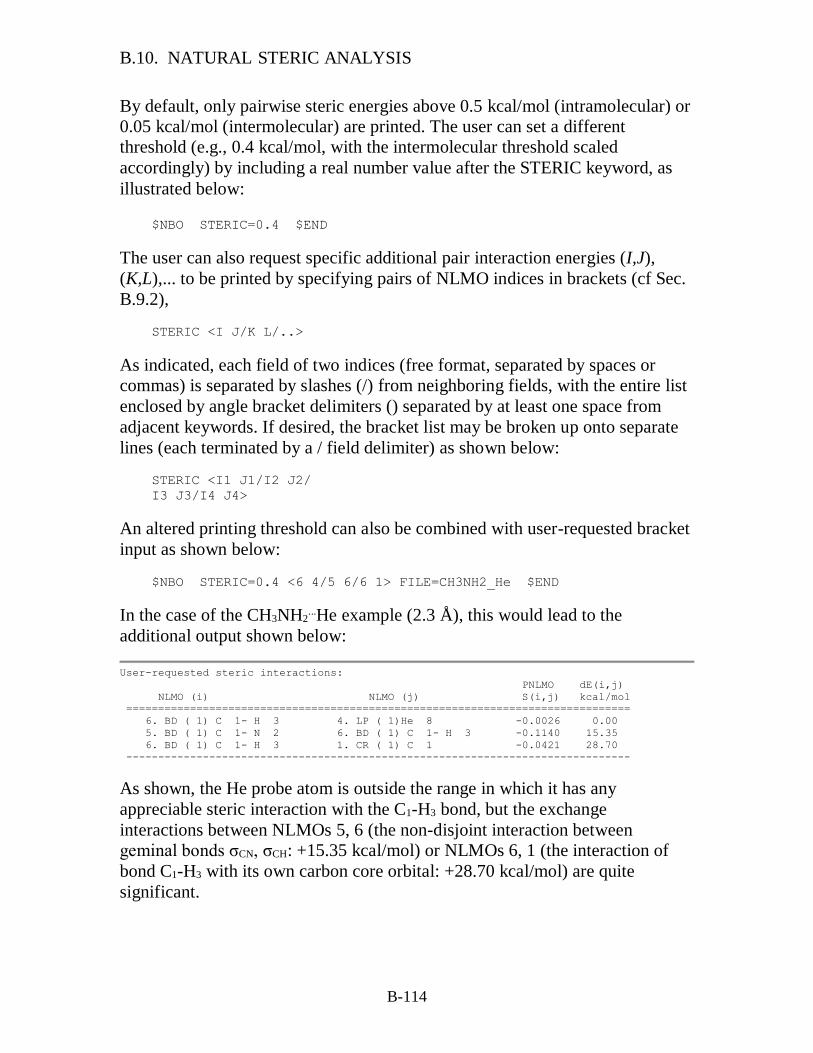

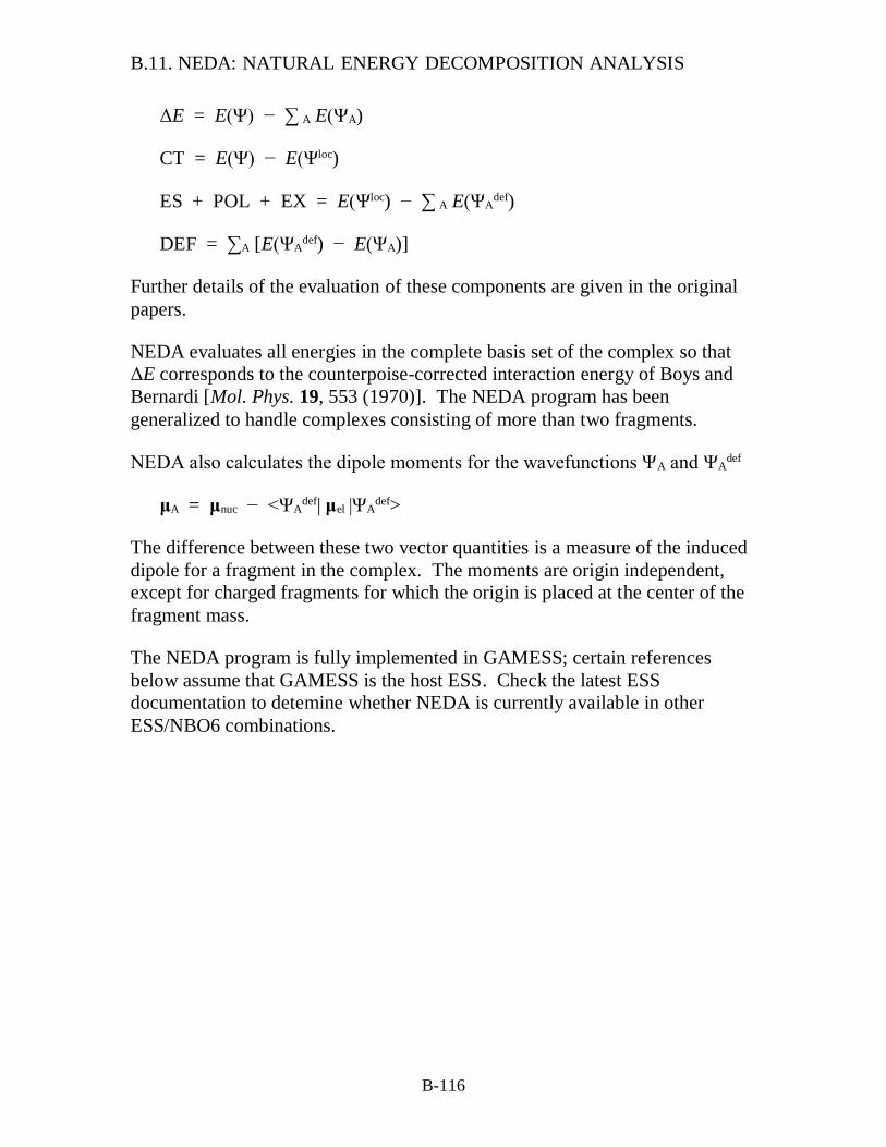
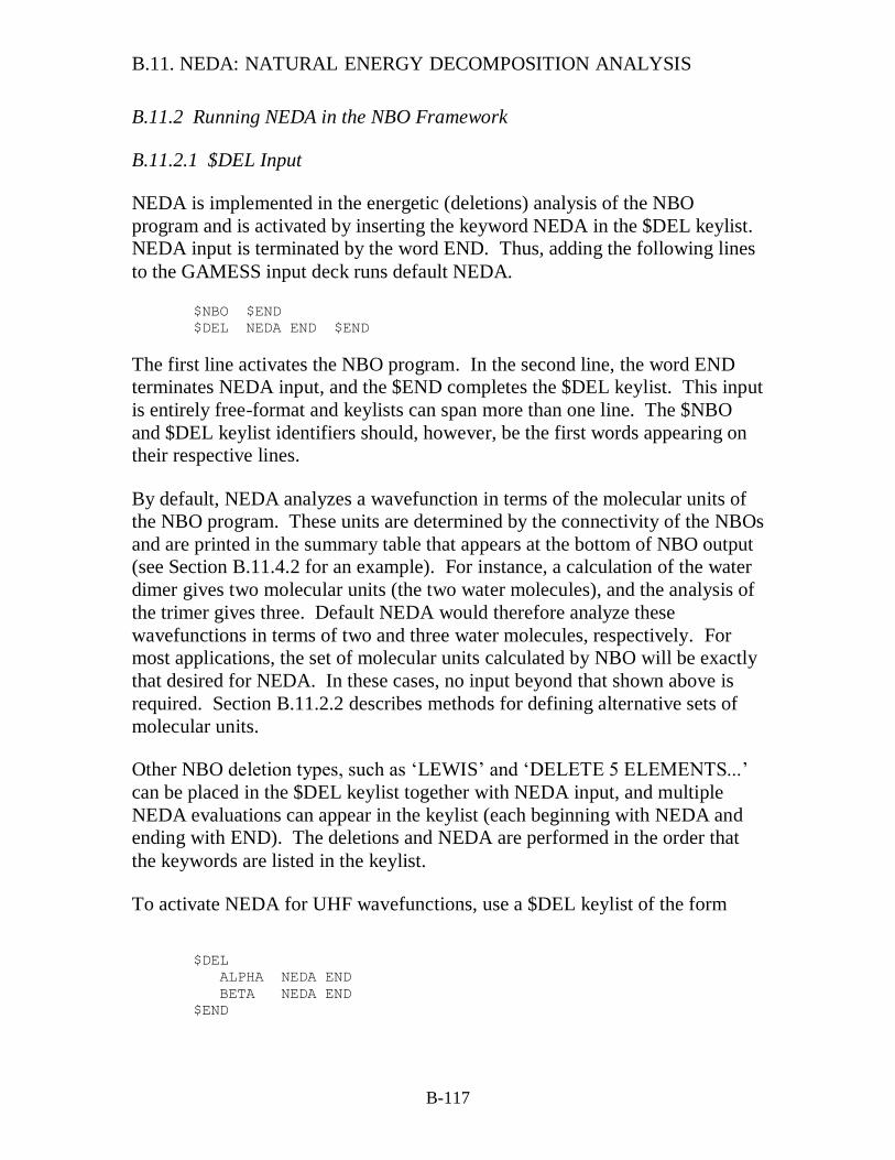
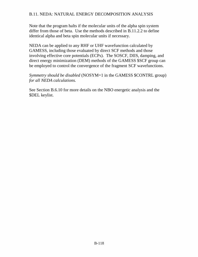
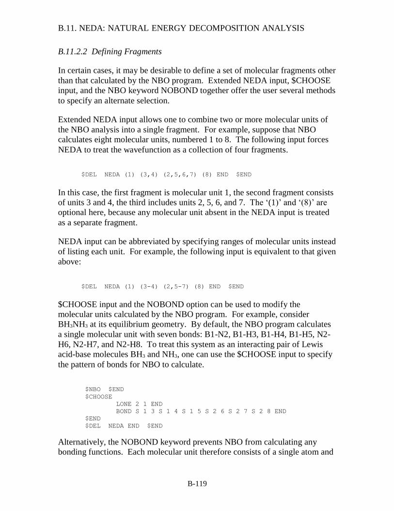
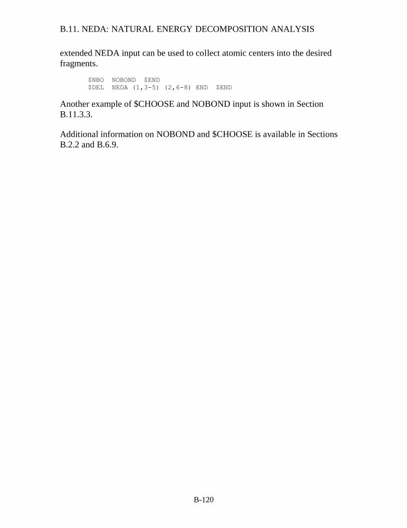
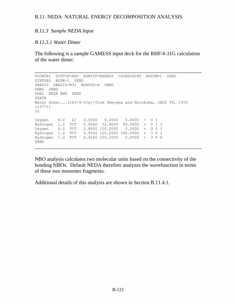
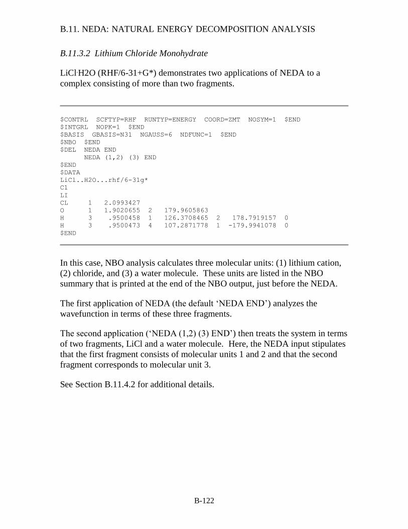
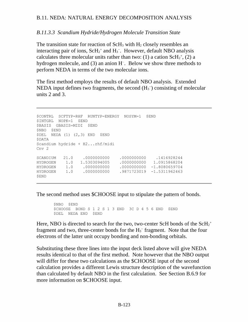
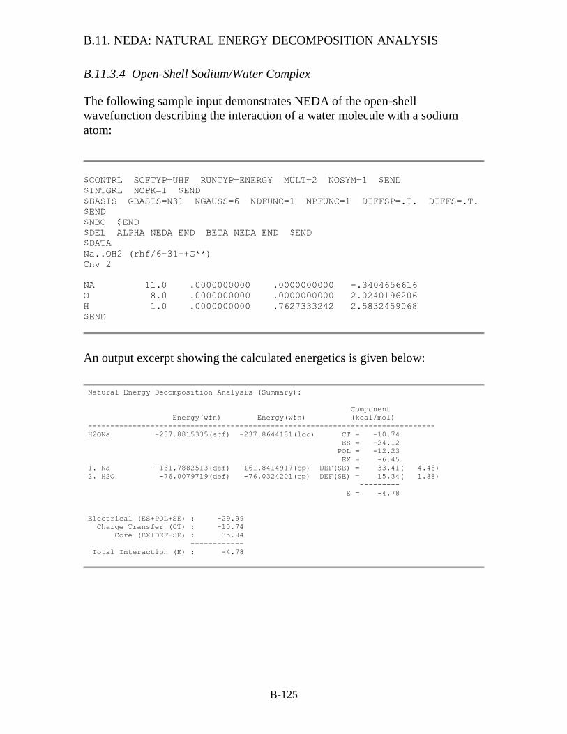
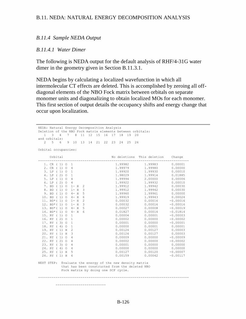
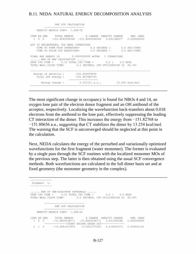
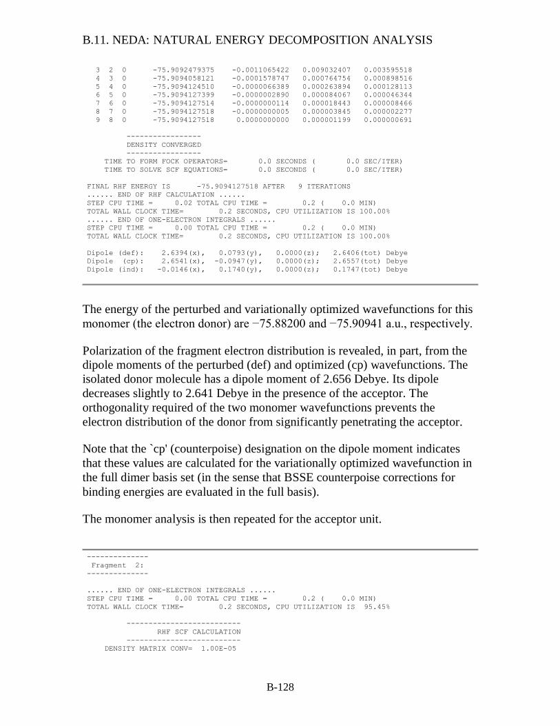
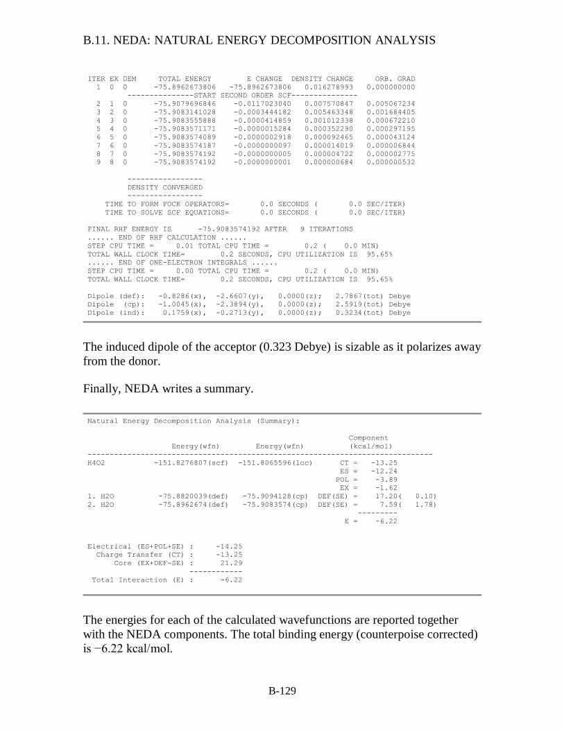
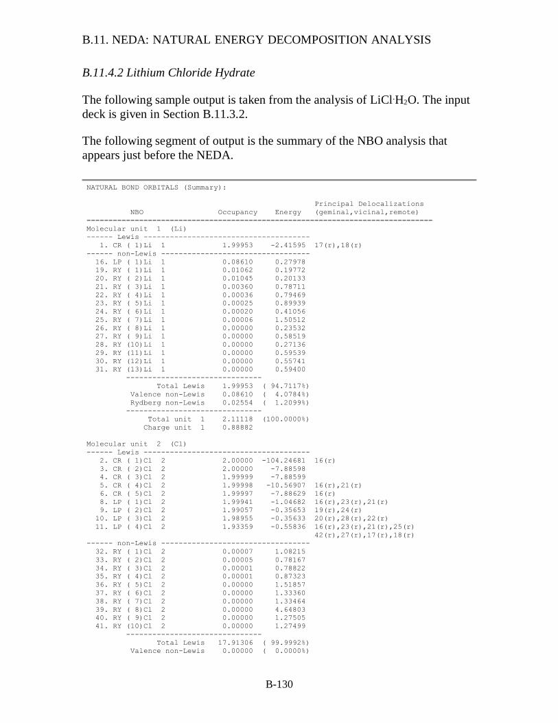
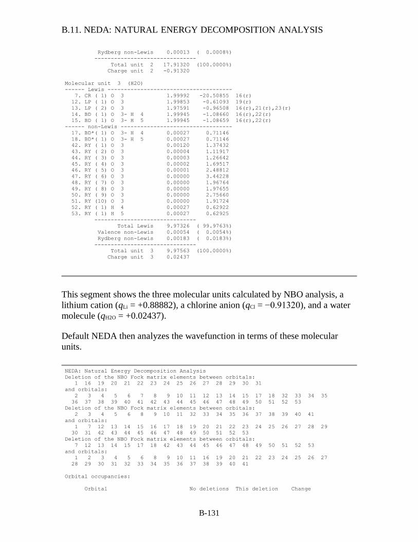
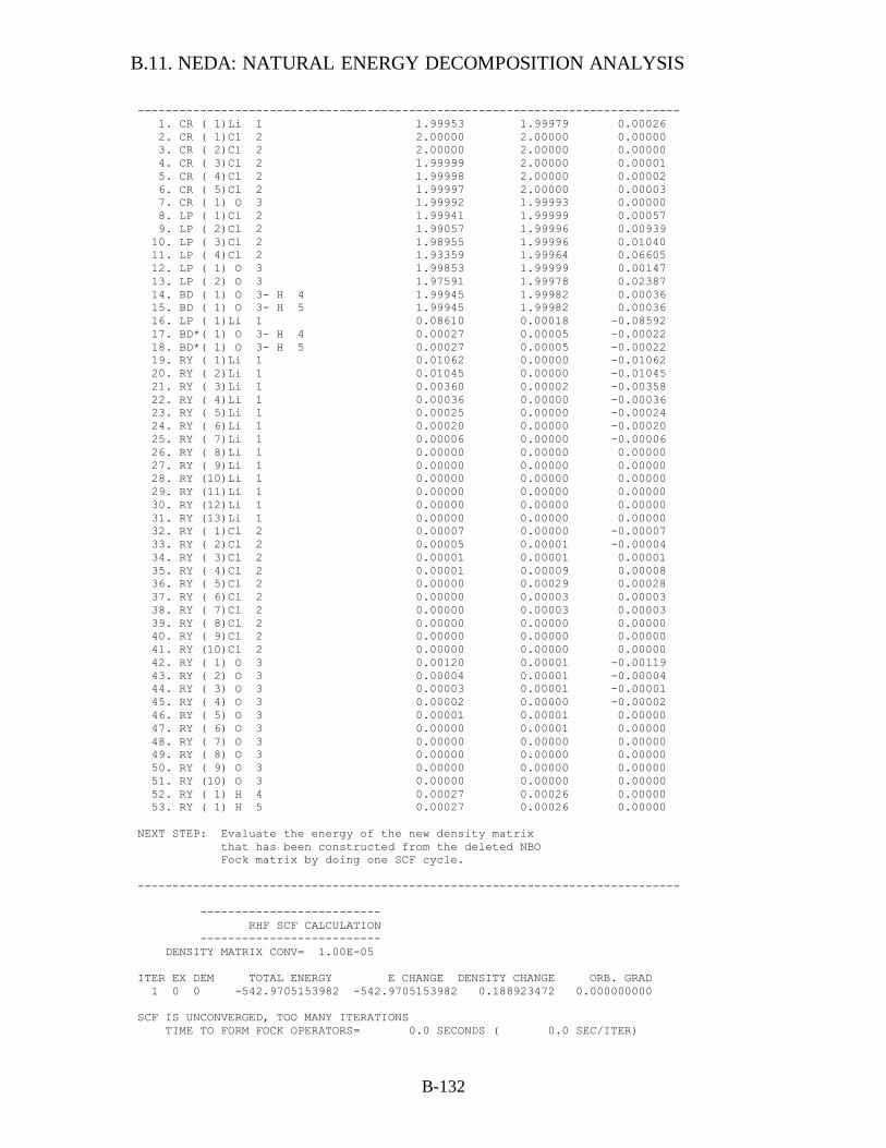

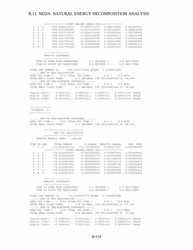
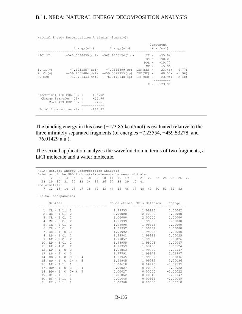


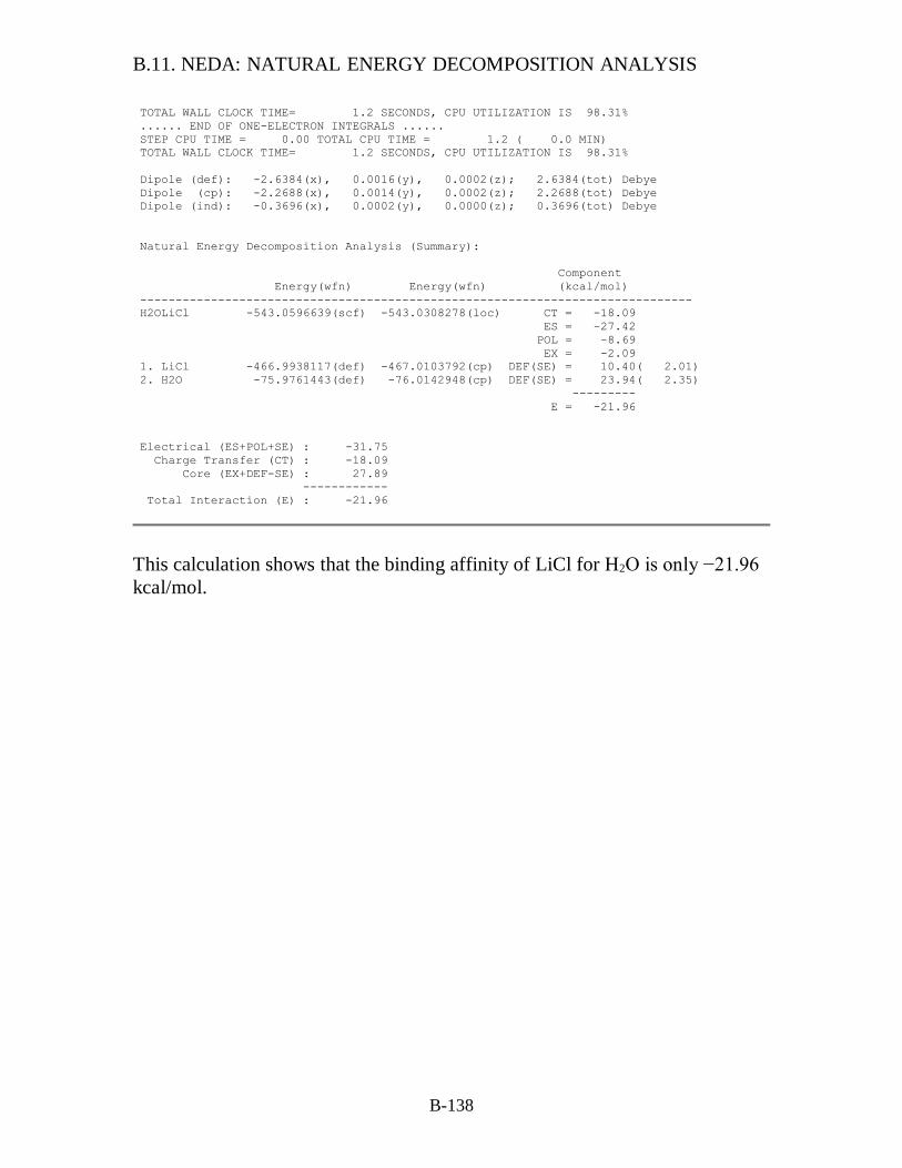

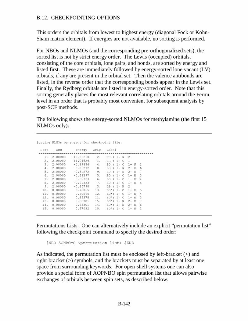
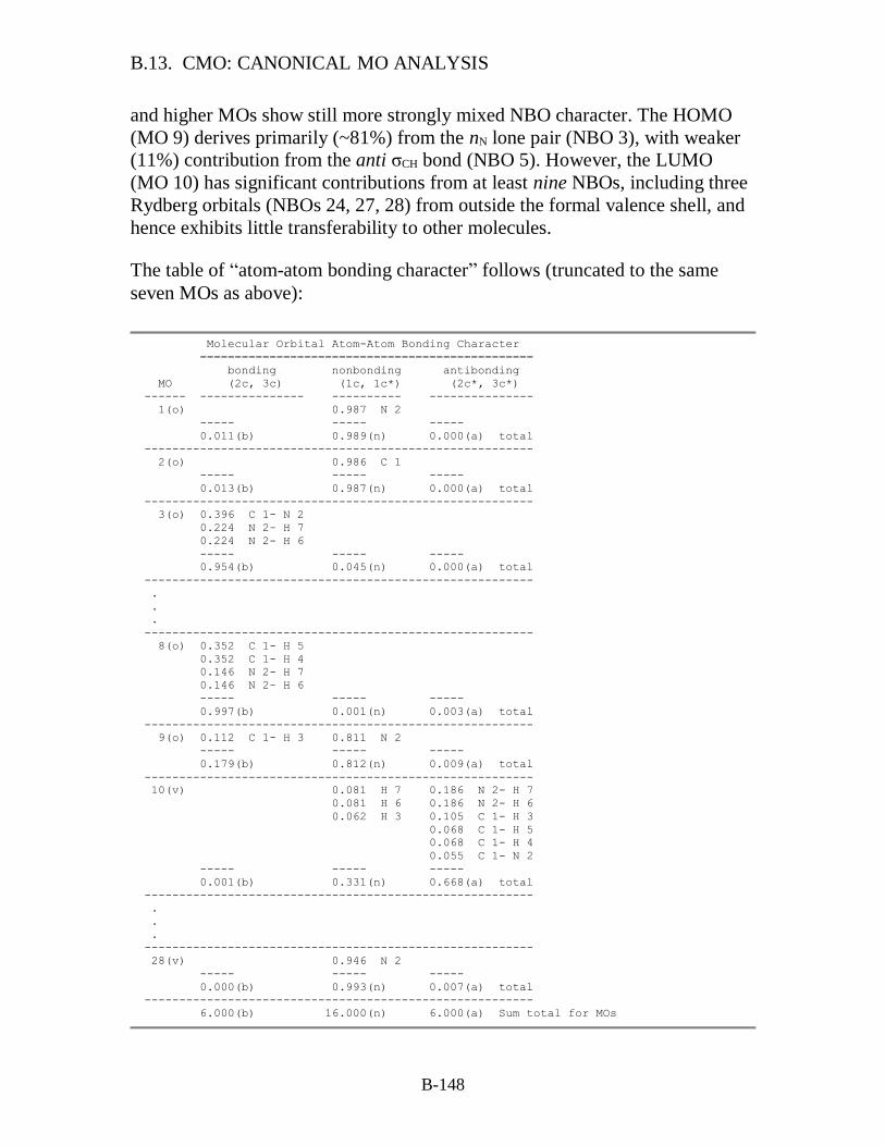

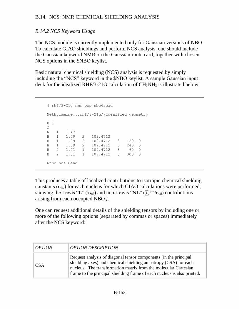
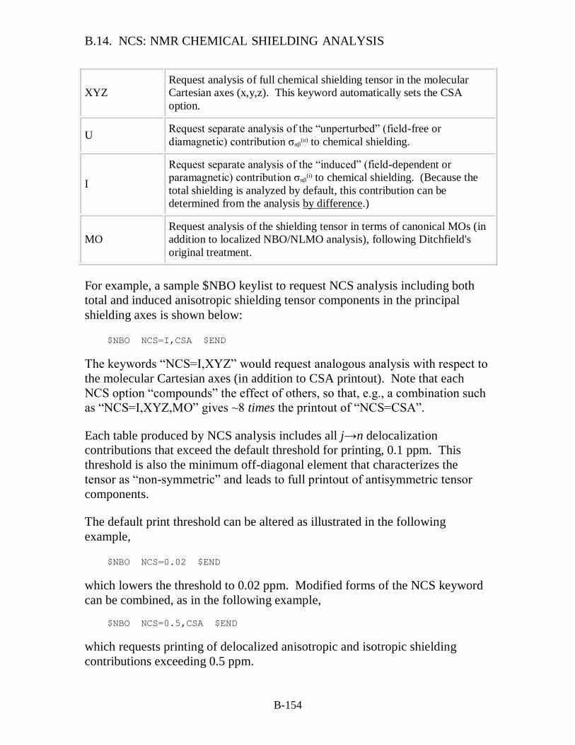

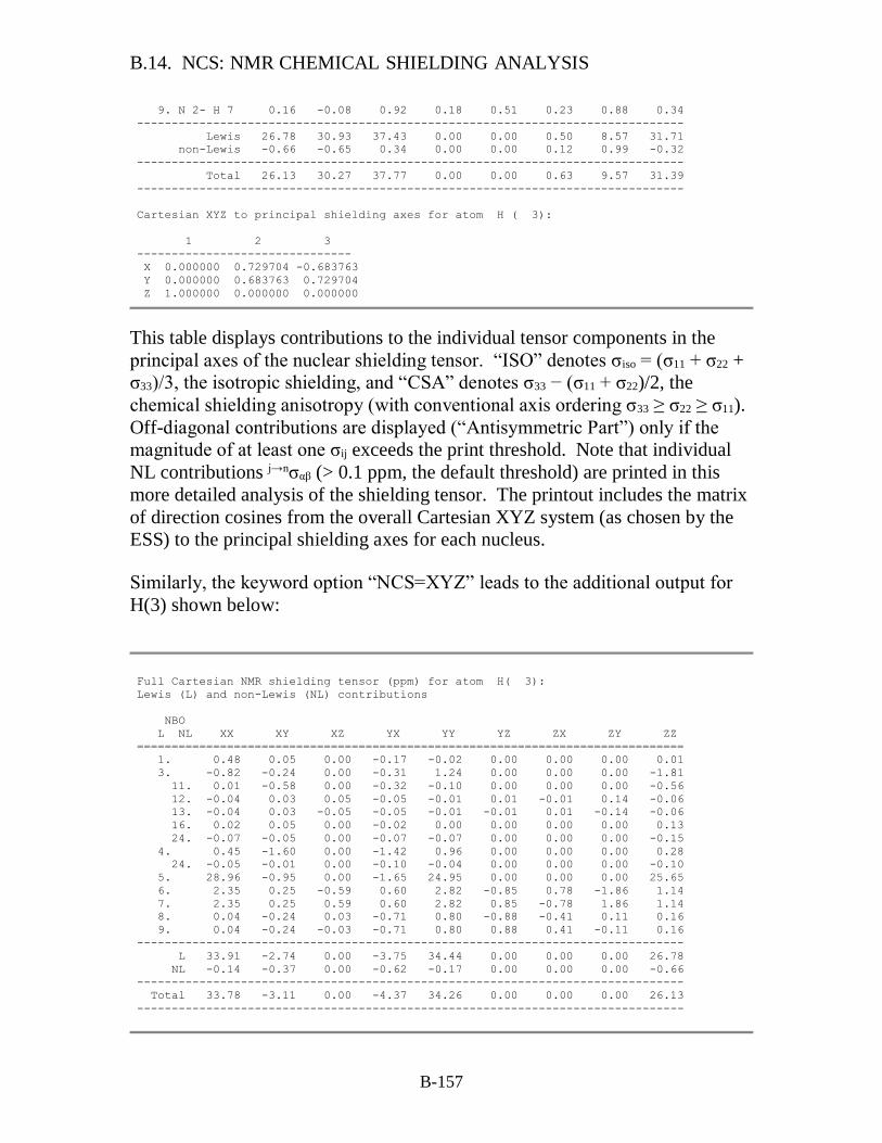
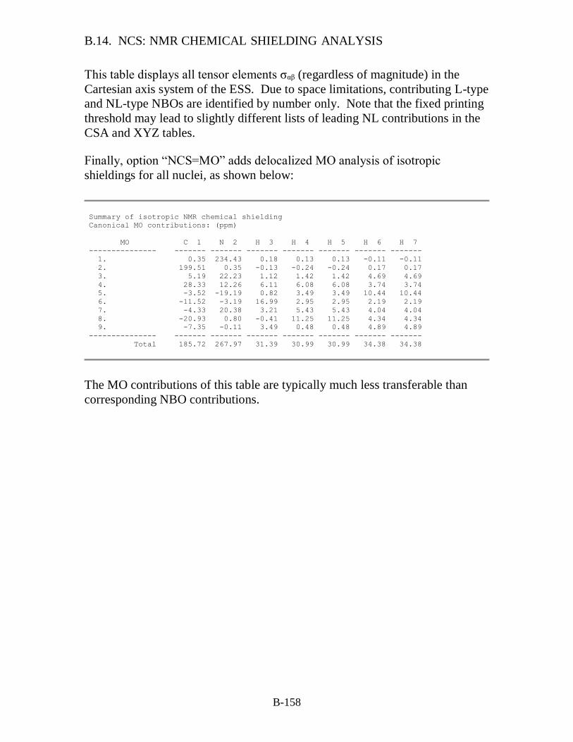

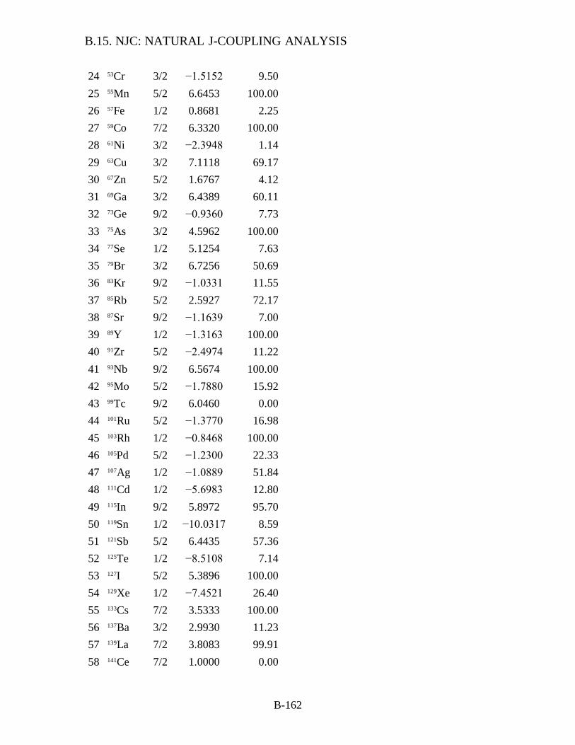

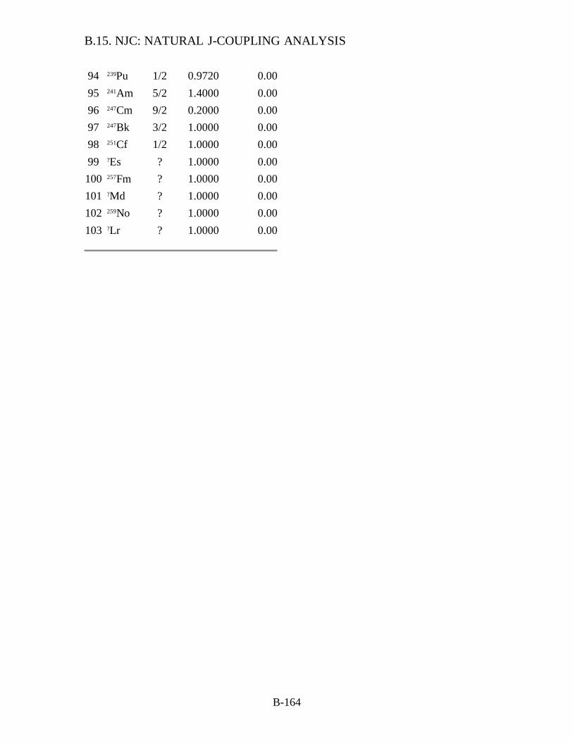
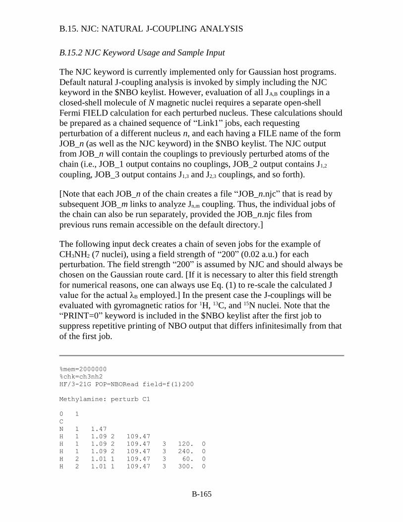
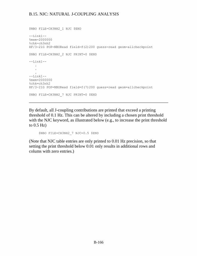
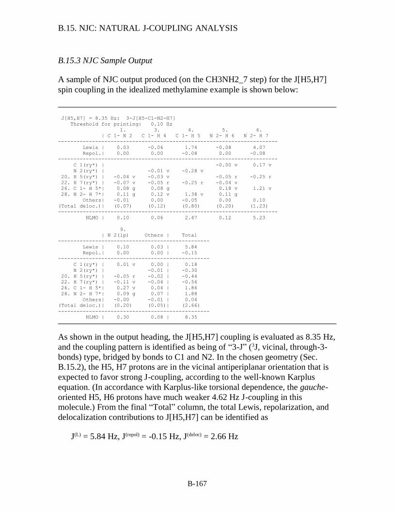
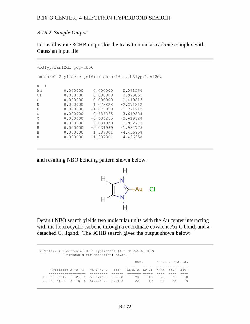

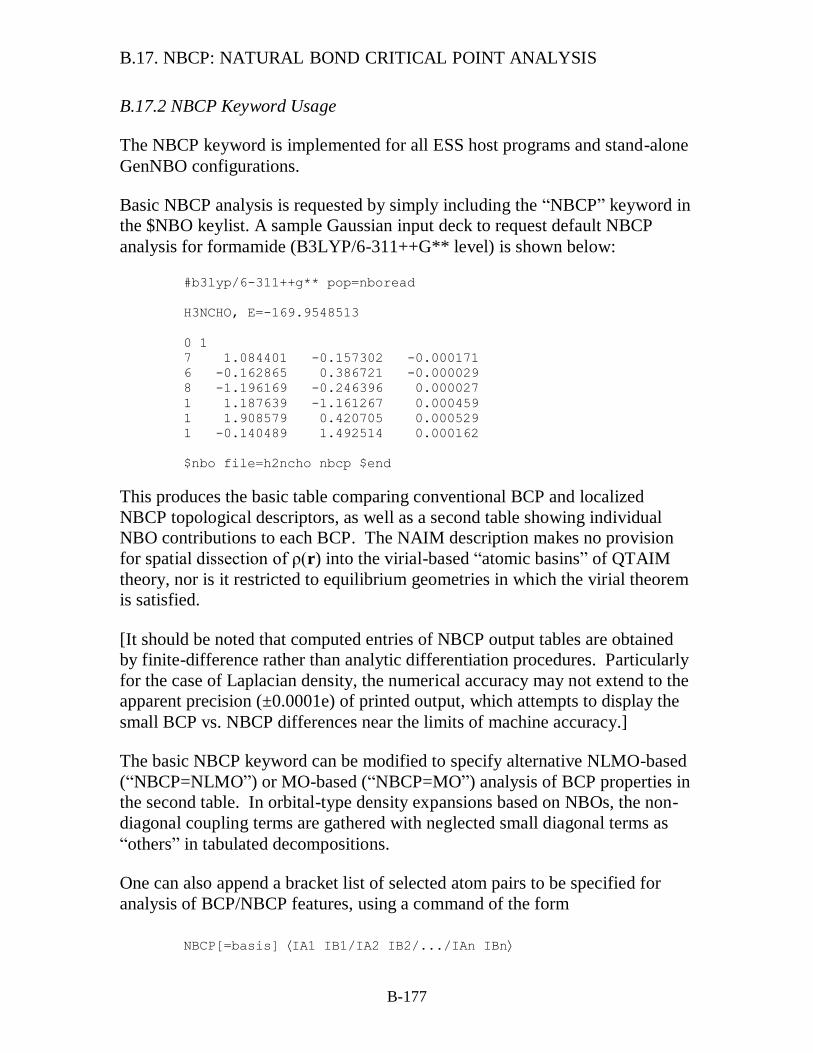

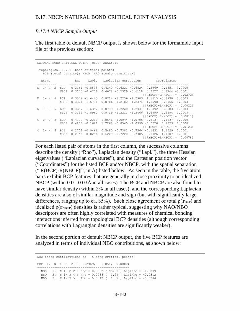
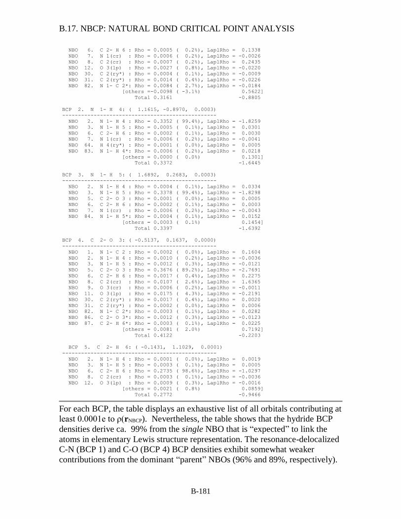
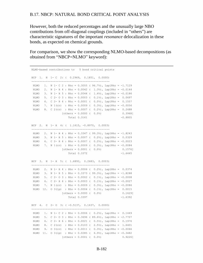
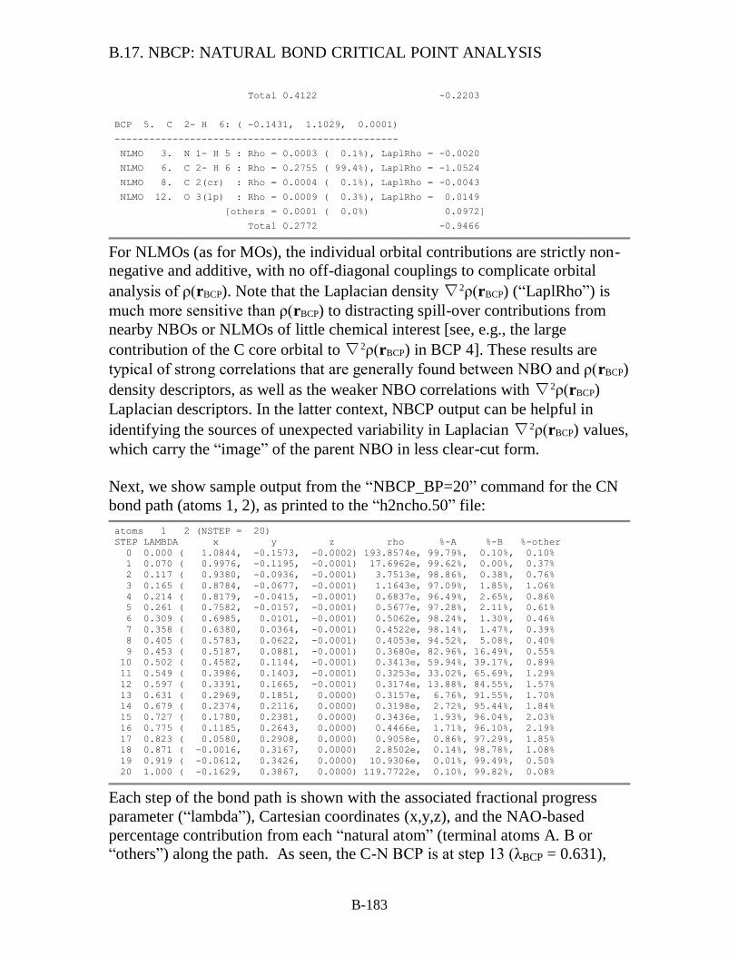

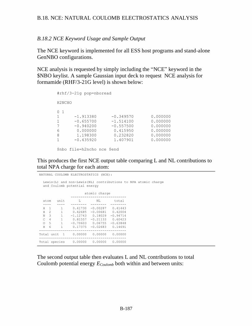
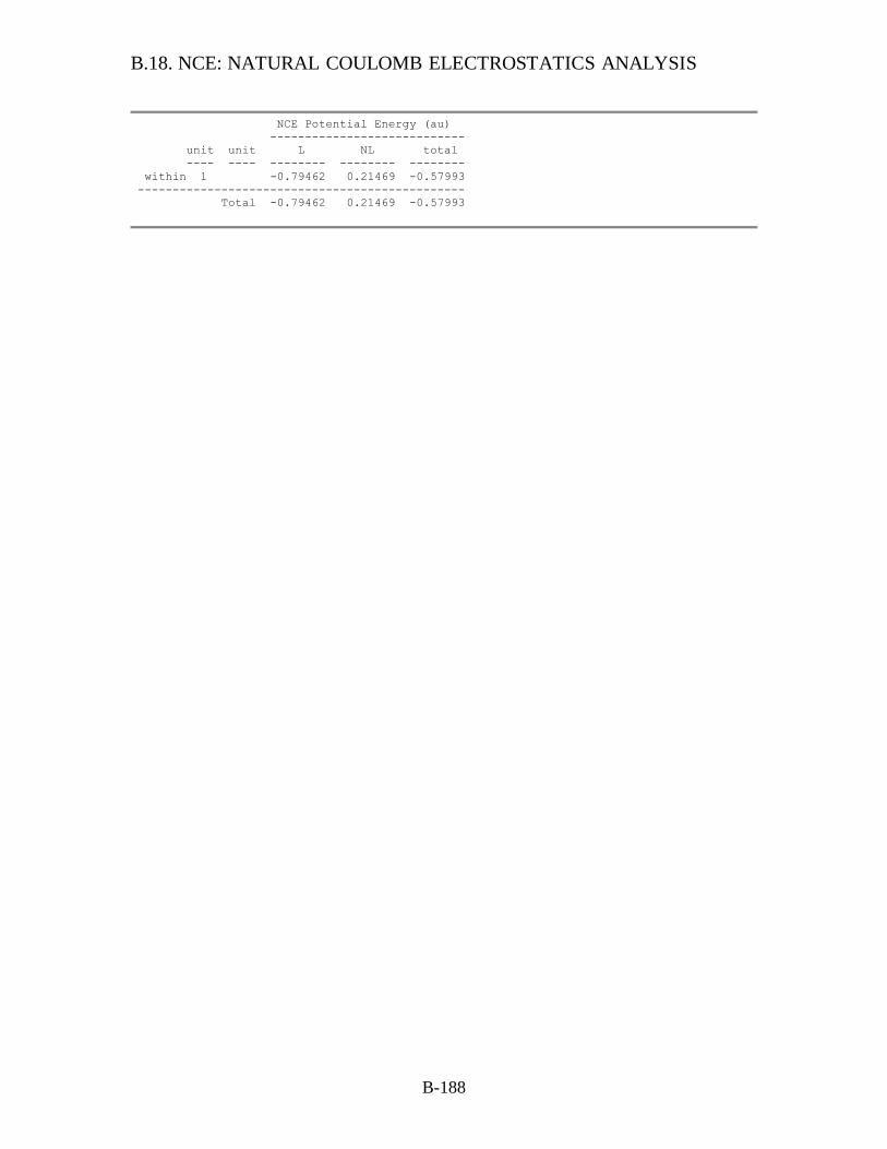

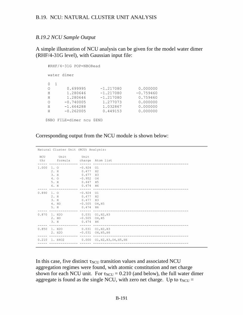
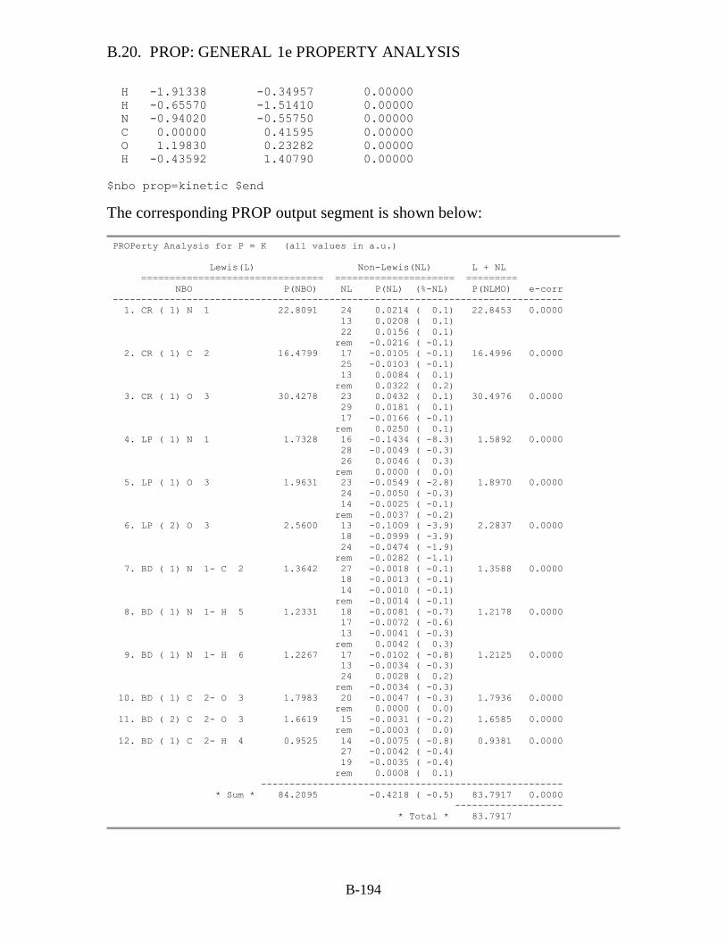

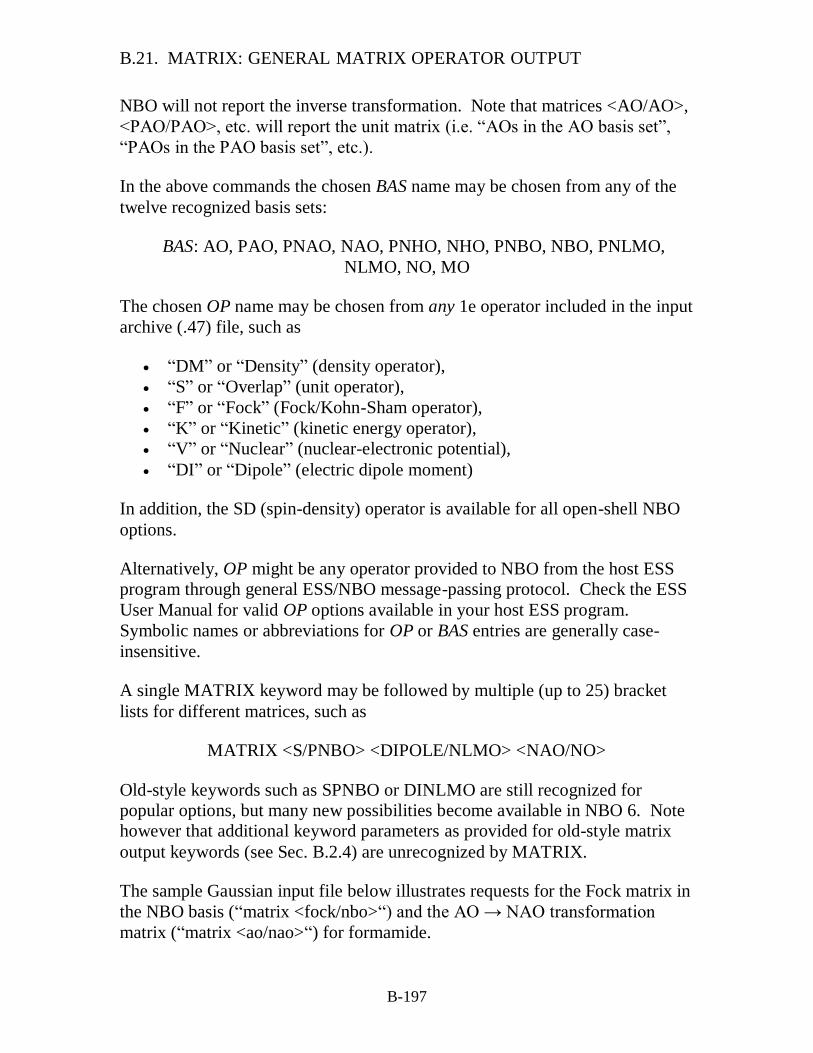
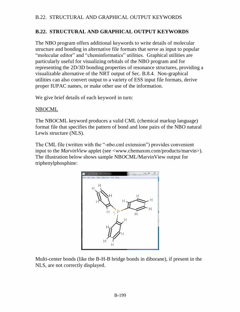
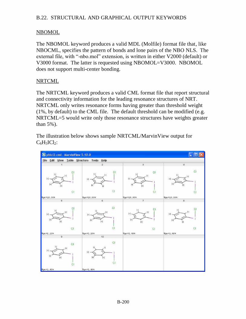
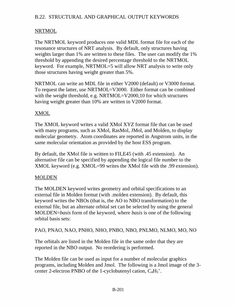
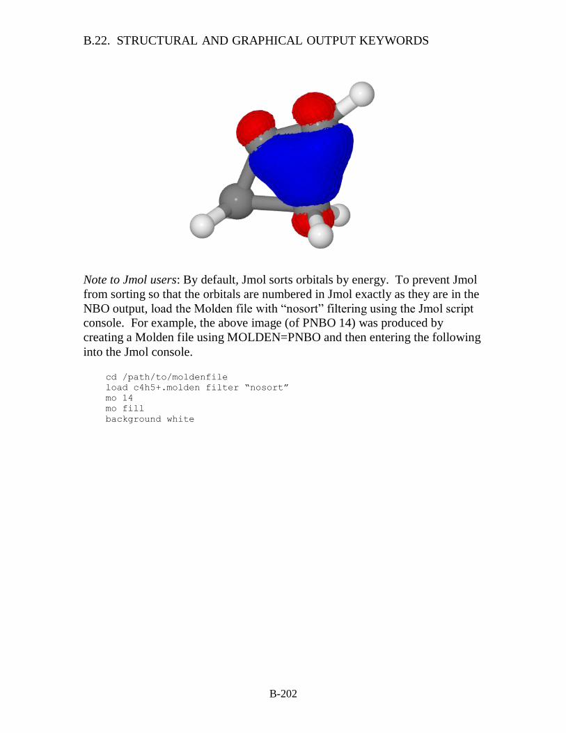
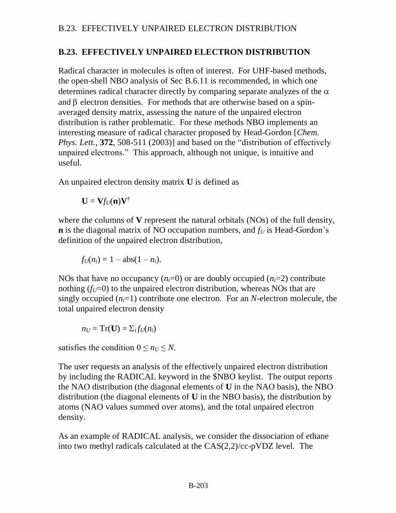

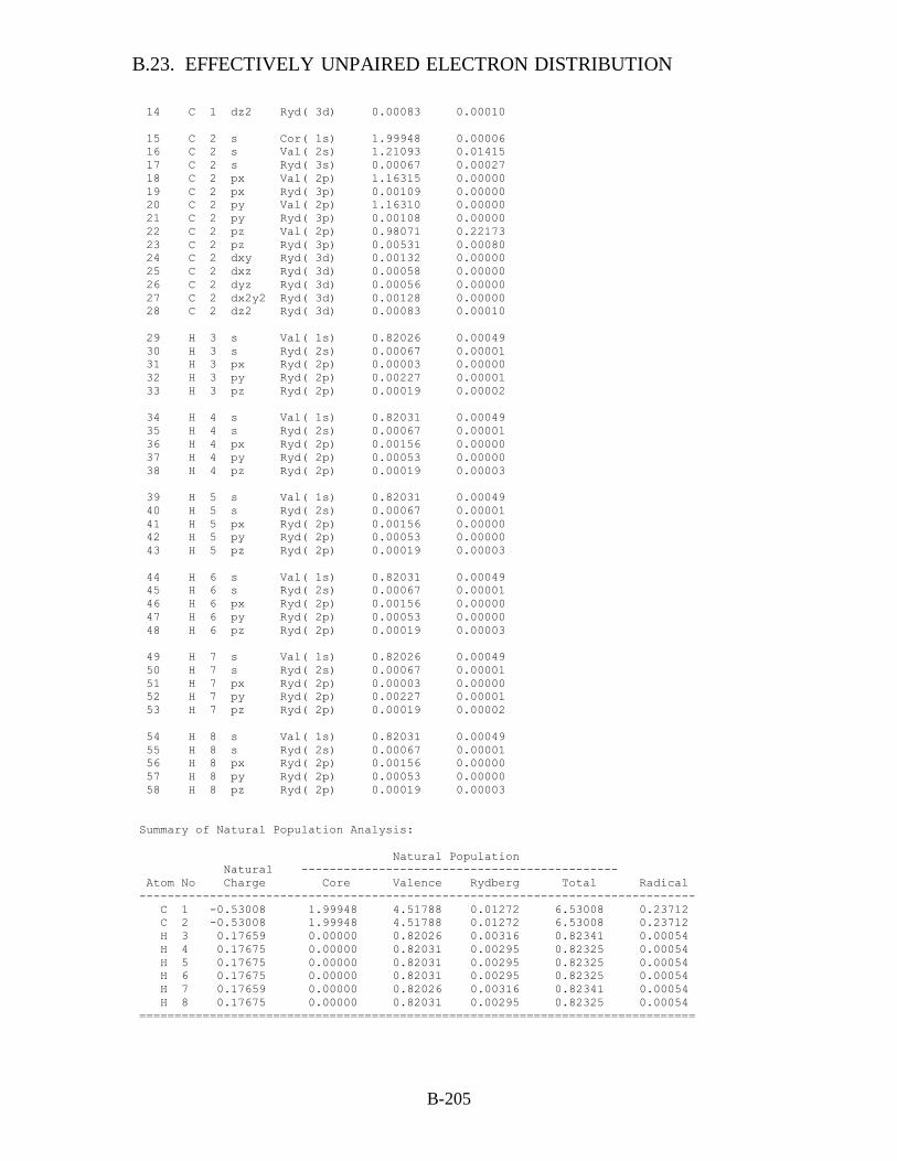

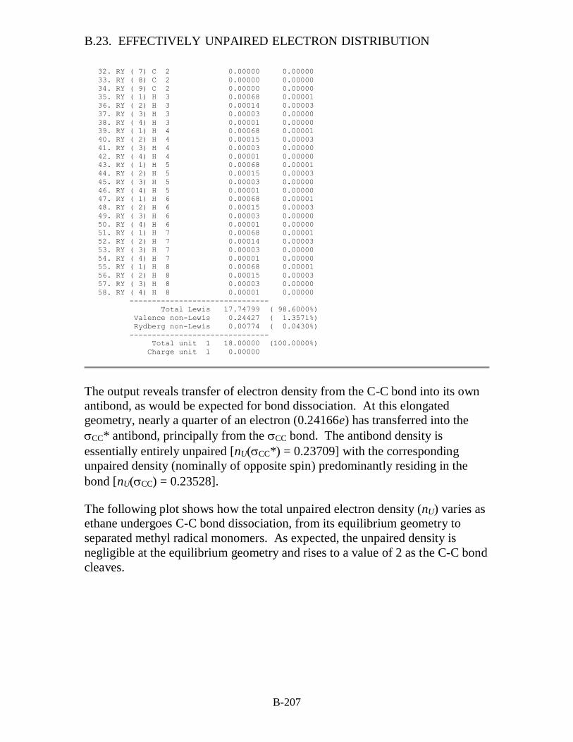
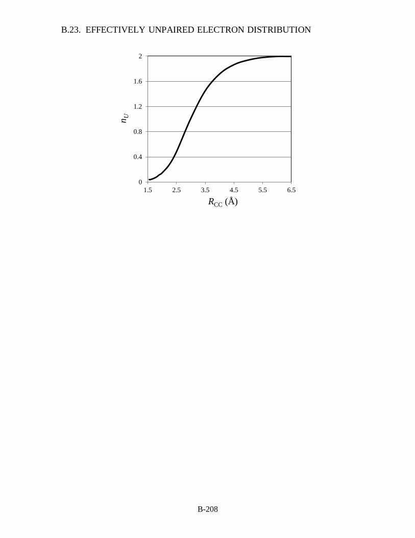


![Freely Available Online Journal of New Developments in ... Natural boding orbital (NBO) ... [17] program package, invoking gradient geometry optimization ... 3.0 Experimental details](https://static.documents.pub/doc/80x56/5b0d06e57f8b9ab7658bcdcc/freely-available-online-journal-of-new-developments-in-boding-orbital-nbo.jpg)


