NCHRP Report 794, Appendices 1 NCHRP Report 794 Median Cross-Section Design for Rural Divided Highways Appendices Appendix A—2003 Survey Questionnaire Appendix B—2006 Survey Questionnaire Appendix C—Crash Sorting Codes Appendix D—Design and Testing of a Terrain Mapping System for Median Slope Measurement Appendix E—Economic Analyses Disclaimer These appendices to NCHRP Report 794 are uncorrected drafts as submitted by the research agency. Any opinions or conclusions expressed and implied in the appendices are those of the research agency. They are not necessarily those of the Transportation Research Board, the National Research Council, the Federal Highway Administration, the American Association of State Highway and Transportation Officials, or of the individual states participating in the National Cooperative Highway Research Program.
Transcript
NCHRP Report 794, Appendices 1
NCHRP Report 794
Median Cross-Section Design for Rural Divided Highways
Appendices
Appendix A—2003 Survey Questionnaire
Appendix B—2006 Survey Questionnaire
Appendix C—Crash Sorting Codes
Appendix D—Design and Testing of a Terrain Mapping System for Median Slope Measurement
Appendix E—Economic Analyses
Disclaimer
These appendices to NCHRP Report 794 are uncorrected drafts as submitted by the research
agency. Any opinions or conclusions expressed and implied in the appendices are those of the
research agency. They are not necessarily those of the Transportation Research Board, the
National Research Council, the Federal Highway Administration, the American Association of
State Highway and Transportation Officials, or of the individual states participating in the
National Cooperative Highway Research Program.
NCHRP Report 794, Appendices 2
NCHRP Report 794, Appendices 3
Appendix A
2003 Survey Questionnaire
NCHRP Report 794, Appendices 4
NCHRP Report 794, Appendices A-1
NCHRP Report 794, Appendices A-2
NCHRP Report 794, Appendices A-3
NCHRP Report 794, Appendices A-4
NCHRP Report 794, Appendices A-5
NCHRP Report 794, Appendices A-6
NCHRP Report 794--Appendices.doc 7
Appendix B
2006 Survey Questionnaire
NCHRP Report 794--Appendices.doc 8
NCHRP Report 794, Appendices B-1
NCHRP Report 794, Appendices B-2
NCHRP Report 794, Appendices B-3
NCHRP Report 794, Appendices B-4
NCHRP Report 794, Appendices B-5
NCHRP Report 794, Appendices B-6
NCHRP Report 794, Appendices B-7
NCHRP Report 794, Appendices B-8
NCHRP Report 794, Appendices B-9
NCHRP Report 794, Appendices B-10
NCHRP Report 794, Appendices B-11
NCHRP Report 794, Appendices B-12
NCHRP Report 794, Appendices B-13
NCHRP Report 794, Appendices B-14
NCHRP Report 794, Appendices B-15
NCHRP Report 794, Appendices B-16
NCHRP Report 794, Appendices B-17
NCHRP Report 794, Appendices B-18
NCHRP Report 794, Appendices 19
Appendix C
Crash Sorting Codes
NCHRP Report 794, Appendices 20
NCHRP Report 794, Appendices C-1
C.1 Process of Categorizing Median Accidents
C.2 California Accident Flags
NCHRP Report 794, Appendices C-2
NCHRP Report 794, Appendices C-3
NCHRP Report 794, Appendices C-4
NCHRP Report 794, Appendices C-5
NCHRP Report 794, Appendices C-6
NCHRP Report 794, Appendices C-7
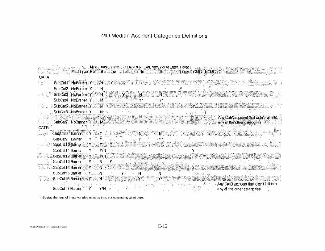
C.3 Missouri Accident Flags
NCHRP Report 794, Appendices C-8
NCHRP Report 794, Appendices C-9
NCHRP Report 794, Appendices C-10
NCHRP Report 794, Appendices C-11
NCHRP Report 794--Appendices.doc C-12
NCHRP Report 794--Appendices.doc C-13
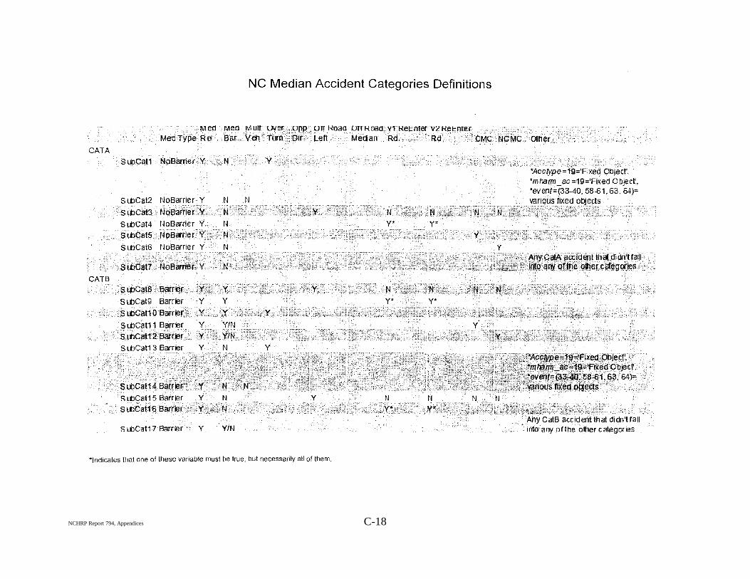
C.4 North Carolina Accident Flags
NCHRP Report 794--Appendices.doc C-14
NCHRP Report 794--Appendices.doc C-15
NCHRP Report 794--Appendices.doc C-16
NCHRP Report 794--Appendices.doc C-17
NCHRP Report 794, Appendices C-18
NCHRP Report 794, Appendices C-19
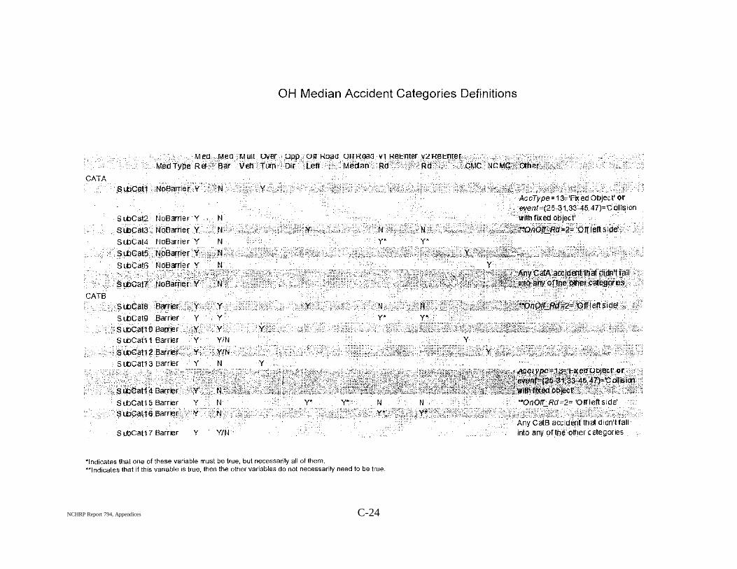
C.5 Ohio Accident Flags
NCHRP Report 794, Appendices C-20
NCHRP Report 794, Appendices C-21
NCHRP Report 794, Appendices C-22
NCHRP Report 794, Appendices C-23
NCHRP Report 794, Appendices C-24
NCHRP Report 794, Appendices C-25
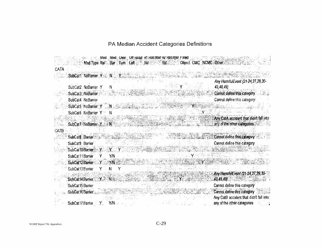
C.6 Pennsylvania Accident Flags
NCHRP Report 794, Appendices C-26
NCHRP Report 794, Appendices C-27
NCHRP Report 794, Appendices C-28
NCHRP Report 794, Appendices C-29
NCHRP Report 794--Appendices.doc C-30
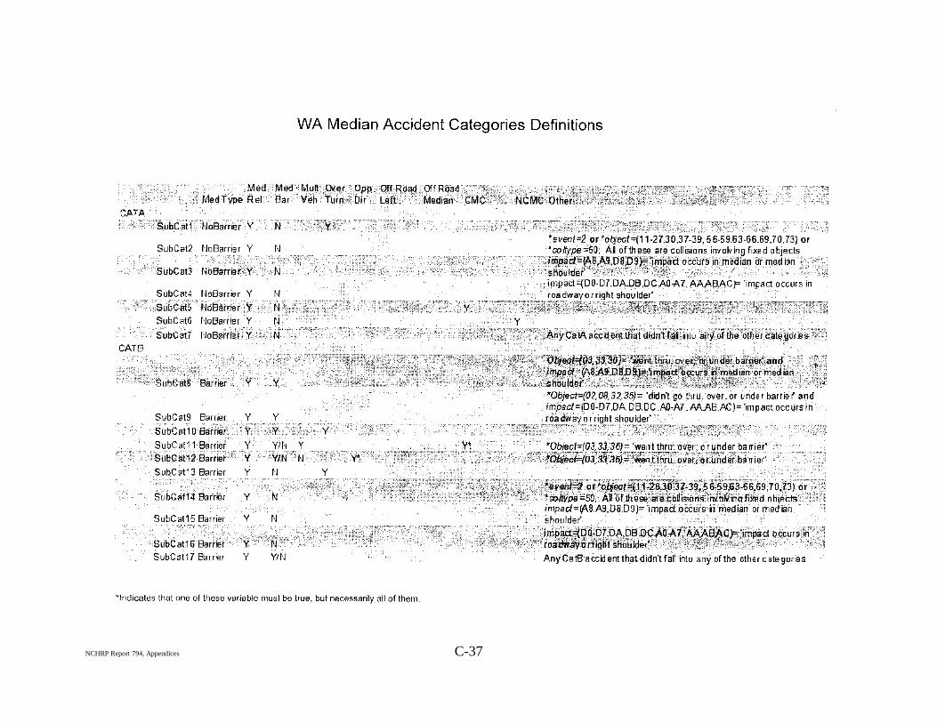
C.7 Washington State Accident Flags
NCHRP Report 794--Appendices.doc C-31
NCHRP Report 794--Appendices.doc C-32
NCHRP Report 794--Appendices.doc C-33
NCHRP Report 794--Appendices.doc C-34
NCHRP Report 794--Appendices.doc C-35
NCHRP Report 794--Appendices.doc C-36
NCHRP Report 794, Appendices C-37
NCHRP Report 794, Appendices C-38
NCHRP Report 794, Appendices 39
Appendix D
Design and Testing of a Terrain Mapping System for Median Slope Measurement
NCHRP Report 794, Appendices 40
NCHRP Report 794, Appendices D-1
D1. Introduction
Median cross-section elements (e.g., width and side-slopes) are critical in determining the
nature of crashes that occur in a median, and selection of cross-sectional elements requires
tradeoffs: “flattened” medians may result in more crossover median crashes, while medians
which have steep slopes might increase the probability of vehicle rollover. The makeup in the
vehicle fleet has also affected aspects of this tradeoff, particularly in regard to rollover. In the
past decades, consumers have purchased a significant number of Sports Utility Vehicles (SUVs)
which have a greater propensity to overturn than some smaller cars. Increased travel speeds and
traffic volumes on the nation’s highways also call to attention the need to make possible changes
to the American Association of State Highway and Transportation Officials (AASHTO) policy
on geometric design of highways and streets, a policy which has remained largely unchanged
over the last many years (1). Median cross-section design also plays a pivotal role in the
selection and evaluation of in-median corrective factors such as median barriers. In particular,
the relative positioning of a median barrier in a median directly affects the nature and number of
crashes that happen in the median.
While there are a number of research projects that seek to find analytical or descriptive
models relating median design to crashes, a key shortcoming is the lack of knowledge of median
cross-section elements on existing roadways. For example, a descriptive method would be to
check for statistical correlation between the median geometry on an existing segment and the
corresponding rollover and crossover crashes that have occurred therein. Or one might use an
analytical approach where one simulates the behavior of different vehicles on an idealized slope
using vehicle dynamics software packages. In both cases, the selection of representative
“idealized” slopes must be motivated by existing median cross-sections, and for most roads, this
information is not readily available.
Careful study of median design clearly requires collection of significant amounts of median
data, a process which in turn requires an easy and reliable method to obtain median cross-section
elements. This report describes the design of an automated Light Detecting and Ranging
(LIDAR) based terrain mapping system which has been used to collect the median profile data
for the study. This automated system satisfies a number of design constraints including:
Use of only off-the-shelf technology.
A portable system that can be shipped to any location for rapid mapping.
Allowing the design to be fitted to any existing large sized SUV without causing any
permanent changes or making any custom modifications to the vehicle.
Developing a simple and intuitive graphic user interface (GUI) to control the equipment
when on the road.
Designing software that can process a huge amount of data collected by the system and
extract relevant median cross-section elements (the adjacent slope and the opposing
slope, and median barrier offset).
Testing the reliability of the system through repeated deployments in a wide range of
roadway conditions.
NCHRP Report 794, Appendices D-2
Testing the repeatability of the system to evaluate expected variability of the data.
Calibrating and conducting error analysis to understand the most common sources of
error and accuracy versus existing methods of median measurement.
This appendix presents a system developed to meet these needs, and in particular details the error
and repeatability analysis aspects of the system design and evaluation process.
NCHRP Report 794, Appendices D-3
D2. Literature Survey
The most common modern practice to survey wide swaths of geometry is the use of LIDAR, and LIDAR-based terrain mapping technology has been demonstrated across a variety of applications. While aerial LIDAR technology has been present for some time and has been extremely useful in survey applications (2), there are some limitations with regard to the level of detail that could be obtained by this means. For example, a recent study by Souleyrette (3) revealed that it was infeasible to extract shoulder slope data from aerial LIDAR because of the narrowness of the shoulder. Road vehicle-based LIDAR mapping technology is another option which typically involves collecting terrain information from LIDARs and Global Positioning System – Inertial Measurement Unit (GPS-IMU) mounted on a vehicle. This approach has the advantage of providing the required amount of detail to accurately measure parameters like the roadway cross-slope, median cross-section elements, etc., but has the disadvantage of complexity in calibration and removing vehicle motion, issues discussed herein. Roadway cross-slope measurement with LIDARs was initially patented by Mekemson (4). It must be noted that this patent delves into measuring the cross-slope of the pavement and is different from the work in this report which looks into measuring the cross-slope of off-road features like medians. In this patent, a ring-laser gyroscope is used to measure the roll of the vehicle with respect to a level datum and the LIDARs, which are placed on either side of a platform extending from the rear of the vehicle, and are used to measure the roll of the vehicle with respect to the pavement. By subtracting out the roll of the vehicle with respect to the pavement from the roll measured from the ring laser gyro, this method is able to measure the cross-slope of the pavement very accurately. In our experiments we have assumed that the roll of the vehicle with respect to the pavement is negligible; this assumption was based on work done by Mraz (5) who has shown that accurate measurement of the cross-slope of the road is possible by simply using a well calibrated GPS-IMU system mounted on a vehicle. Some of the other applications for which LIDAR based mapping has been used are in road profilometry to measure pavement ride quality (6)(7)(8)(9)(10)(11). These applications typically use high frequency and high accuracy LIDAR systems that usually measure the pavement surface from close proximity (6 to 10 in off the ground) and determine the smoothness of the pavement and thereby access whether it meets ride quality standards. Active research is also being conducted in terrain mapping with the aid of LIDARs for its applications in robotics (12)(13)(14). The methods of LIDAR terrain mapping in robotics are typically focused on detecting and extracting the obstacles in the path of the robot by processing the LIDAR data, but in this application we are more concerned about how accurately the LIDAR is measuring the median cross-sectional elements.
Another method of terrain mapping is to utilize additional sensors like cameras on the vehicles. This provides interesting opportunities to fuse the information obtained from multiple sensors (15)(16), and vision sensors can also be used to extract interesting features such as road conditions (17), lane markers, etc. An example combining vision and LIDAR sensors to obtain road and off-road features for road safety has been presented by the ARRB group (18)(19). Unfortunately, this data collection is still in its infancy, and robust algorithms do not yet exist for highly accurate 3D mapping using vision systems.
While one may see parallels in some of the above work and the work presented in this report, it is important to note that this is the first time a detailed study has been performed to investigate the feasibility of utilizing a terrain based LIDAR scanning system for the purpose of measuring off-road features such as median slopes.
NCHRP Report 794, Appendices D-4
NCHRP Report 794, Appendices D-5
D3. Data Acquisition System
The sensors present in a typical terrain mapping vehicle are a LIDAR, a GPS, and an IMU.
While the LIDAR scans the environment and provides the terrain information relative to the
vehicle, the global position of the vehicle is measured at relatively long intervals by the GPS.
The orientation and fine motion of the vehicle is measured by the IMU. One can observe that a
particular challenge to operate mobile mapping systems is to obtain very accurate position and
orientation information at very high bandwidth by fusion of GPS and IMU data, a process which
requires high accuracy and high-bandwidth IMU’s. Only within the past decade have such units
been available at reasonable cost and outside of defense applications.
To measure information from these three sensors simultaneously, an integrated data
acquisition system is needed. Such a system was developed for NCHRP Project 22-21
(Figure D-1, Figure D-2), and the resulting unit is a portable instrument frame that has been
designed to acquire data from multiple sensors simultaneously. The main aspects of the system
including power electronics, sensor systems, data routing architecture, and data acquisition
software are described below.
Power Electronics
A key problem with mobile data acquisition, particularly with a high-power LIDAR scanner,
is the issue of power quality. To solve this, a complete stand-alone power system was developed
alongside the data-collection system. A two-level design of the instrument frame was adopted to
separate the power electronics systems from the sensor and the computer systems; the power
circuitry is located on the bottom level. This system basically combines the power input from the
on-board battery packs and the vehicle’s alternator to provide well-regulated output independent
of the highly variable vehicle power system.
Table D-1. Processing Portion of the Data Acquisition System
NCHRP Report 794, Appendices D-6
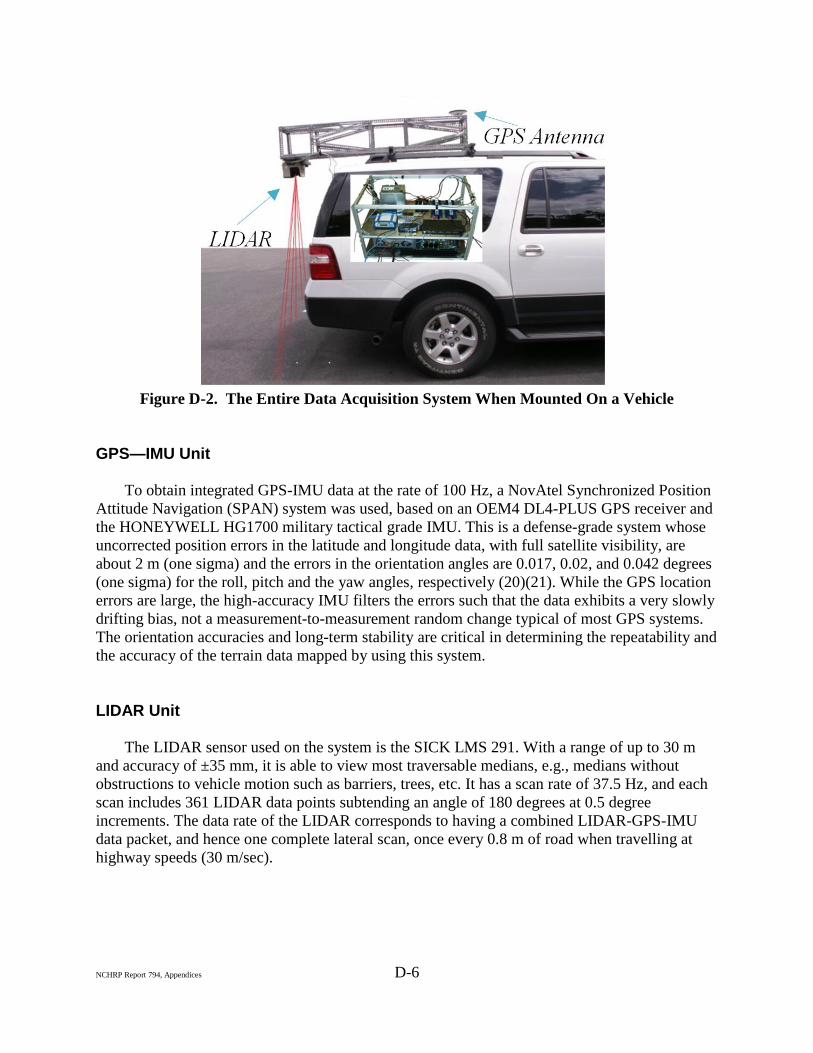
Figure D-2. The Entire Data Acquisition System When Mounted On a Vehicle
GPS—IMU Unit
To obtain integrated GPS-IMU data at the rate of 100 Hz, a NovAtel Synchronized Position
Attitude Navigation (SPAN) system was used, based on an OEM4 DL4-PLUS GPS receiver and
the HONEYWELL HG1700 military tactical grade IMU. This is a defense-grade system whose
uncorrected position errors in the latitude and longitude data, with full satellite visibility, are
about 2 m (one sigma) and the errors in the orientation angles are 0.017, 0.02, and 0.042 degrees
(one sigma) for the roll, pitch and the yaw angles, respectively (20)(21). While the GPS location
errors are large, the high-accuracy IMU filters the errors such that the data exhibits a very slowly
drifting bias, not a measurement-to-measurement random change typical of most GPS systems.
The orientation accuracies and long-term stability are critical in determining the repeatability and
the accuracy of the terrain data mapped by using this system.
LIDAR Unit
The LIDAR sensor used on the system is the SICK LMS 291. With a range of up to 30 m
and accuracy of ±35 mm, it is able to view most traversable medians, e.g., medians without
obstructions to vehicle motion such as barriers, trees, etc. It has a scan rate of 37.5 Hz, and each
scan includes 361 LIDAR data points subtending an angle of 180 degrees at 0.5 degree
increments. The data rate of the LIDAR corresponds to having a combined LIDAR-GPS-IMU
data packet, and hence one complete lateral scan, once every 0.8 m of road when travelling at
highway speeds (30 m/sec).
NCHRP Report 794, Appendices D-7
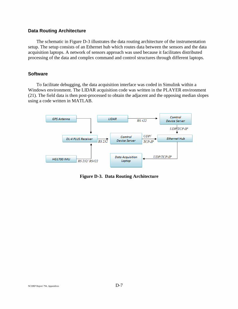
Data Routing Architecture
The schematic in Figure D-3 illustrates the data routing architecture of the instrumentation
setup. The setup consists of an Ethernet hub which routes data between the sensors and the data
acquisition laptops. A network of sensors approach was used because it facilitates distributed
processing of the data and complex command and control structures through different laptops.
Software
To facilitate debugging, the data acquisition interface was coded in Simulink within a
Windows environment. The LIDAR acquisition code was written in the PLAYER environment
(21). The field data is then post-processed to obtain the adjacent and the opposing median slopes
using a code written in MATLAB.
Figure D-3. Data Routing Architecture
NCHRP Report 794, Appendices D-8
NCHRP Report 794, Appendices D-9
D4. Data Processing Algorithm
Each scan contains within it information that provides estimates of the adjacent and the
opposing slope, but extraction of this information is not trivial. The task of the data processing
algorithm can be broken down into four main parts:
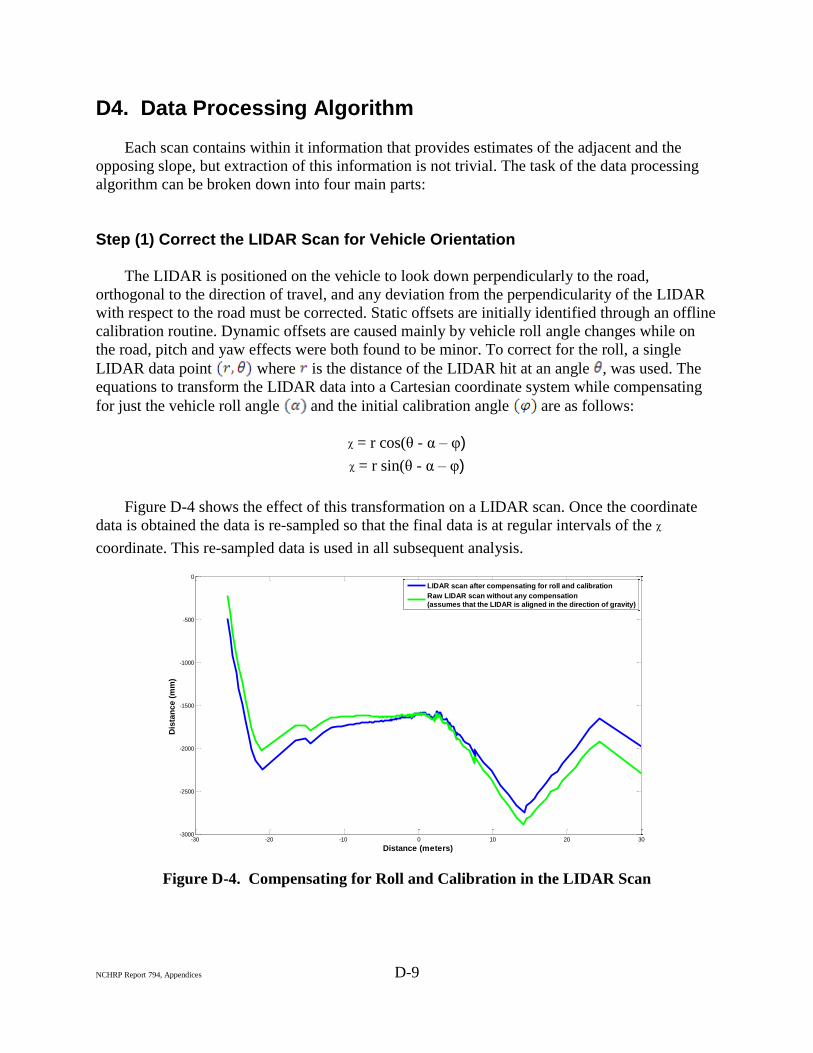
Step (1) Correct the LIDAR Scan for Vehicle Orientation
The LIDAR is positioned on the vehicle to look down perpendicularly to the road,
orthogonal to the direction of travel, and any deviation from the perpendicularity of the LIDAR
with respect to the road must be corrected. Static offsets are initially identified through an offline
calibration routine. Dynamic offsets are caused mainly by vehicle roll angle changes while on
the road, pitch and yaw effects were both found to be minor. To correct for the roll, a single
LIDAR data point where is the distance of the LIDAR hit at an angle , was used. The
equations to transform the LIDAR data into a Cartesian coordinate system while compensating
for just the vehicle roll angle and the initial calibration angle are as follows:
ᵡ = r cos(θ - α – φ)
ᵡ = r sin(θ - α – φ)
Figure D-4 shows the effect of this transformation on a LIDAR scan. Once the coordinate
data is obtained the data is re-sampled so that the final data is at regular intervals of the ᵡ coordinate. This re-sampled data is used in all subsequent analysis.
Figure D-4. Compensating for Roll and Calibration in the LIDAR Scan
-30 -20 -10 0 10 20 30-3000
-2500
-2000
-1500
-1000
-500
0
Distance (meters)
Dis
tan
ce (
mm
)
LIDAR scan after compensating for roll and calibration
Raw LIDAR scan without any compensation
(assumes that the LIDAR is aligned in the direction of gravity)
NCHRP Report 794, Appendices D-10
Step (2) Identify the Road and Road Edge
As the LIDAR is setup perpendicular to the road, the LIDAR data points obtained from
immediately underneath the LIDAR are assumed to be from the road. These form a very smooth
line up to the point of the road edge, and by applying regression, a road line ( ) is identified.
Once the road line is identified (Figure D-5), the edge of the road must be inferred and
because this determination is based on LIDAR data, it might not be the true road edge. A
definition to arrive at the edge of the road from the LIDAR data points, given the equation for
the line of the road, has been formulated by incorporating multiple thresholds as a single
threshold. The definition uses the metric which is the perpendicular
distance of a point from a line . The definition presented here has been
used in computing the edge of the adjacent and the opposing slopes as well. We also define the
Point of Significant Departure : Given a set of n points where and
. Suppose there exists a line and there exists , such that
is the smallest value that satisfies.
Then the PSD is defined as the point where and is the smallest value that
satisfies.
where and are empirically determined thresholds and is set lower
than . The road edge is defined as the of the road line. The values of 75, 30, and
25 mm were used, for thre1, thre2, and thre3, respectively, in order to calculate the road edge.
Figure D-5. The Figure Shows the Identification of a Road Line and the Associated Edge
of the Road by Using that Lane
-10 -5 0 5 10 15 20-3000
-2500
-2000
-1500
Distance (meters)
Dis
tan
ce (
mm
)
LIDAR SCAN
ROAD LINE
EDGE OF THE ROAD
(PSD OF THE ROAD LINE)
NCHRP Report 794, Appendices D-11
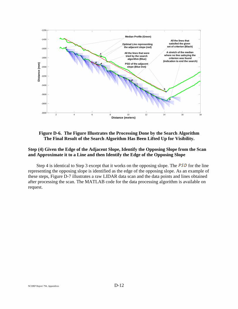
Step (3) Given the Road Edge, Identify the Adjacent Slope from the Scan and Approximate
it to a Line and then Identify the Edge of the Adjacent Slope
The search algorithm starts from the road edge and considers small windows of data,
repeatedly fitting lines to these windows and testing whether the road segment has ended within
the window. Details of this are as follows: within each window, the algorithm finds the point in
that stretch whose height is the statistical median of all the heights within the window. The slope
of the tangent to the profile at this point is calculated using regression. The slope of this tangent
is varied by small increments, creating a family of candidate lines. These candidates are reduced
to a small number of “best fit” lines based on a set of criterion, presented below. Each line that
satisfies the criterion is characterized by the mean of an optimization function which calculates
the number of points whose perpendicular distance from the line is less than a threshold
(25 mm). This process is repeated along the whole median until no lines satisfying the above
criteria are found. Figure D-6 illustrates this process. The candidate lines are shown in blue and
those lines which match the set of criteria are shown in black. We can see that, as we reach
closer to the end of the adjacent slope, the number of black lines decreases until there are none
that satisfy the criterion. At this point, the search is terminated. Once the search is terminated, the
line having the optimal value, e.g., the most points fit by that line across the entire slope, is
selected as the adjacent slope (red line), the of the line is selected as the edge of the
adjacent slope.
The set of criterion used to select a line are as follows:
The for the line is identified and the line is checked to confirm that the length of the
data segment fitting this line is within reasonable limits (between 1.5 m and 10 m).
If the slope of the line is not within a reasonable limit (between 4 degrees and 18
degrees), the line is eliminated.
If the perpendicular distance of any point between the road edge and the for the line
is beyond a certain threshold (250mm) away from the line, the line is considered to have
an obstruction and is eliminated.
NCHRP Report 794, Appendices D-12
Figure D-6. The Figure Illustrates the Processing Done by the Search Algorithm
The Final Result of the Search Algorithm Has Been Lifted Up for Visibility.
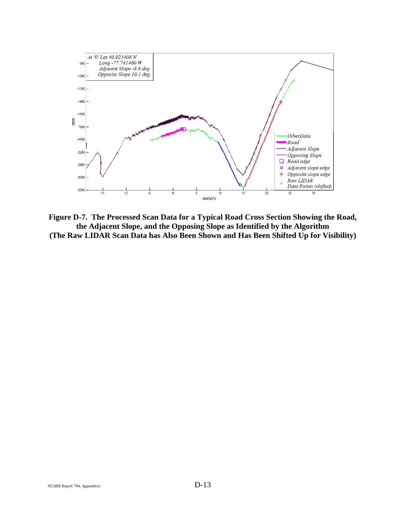
Step (4) Given the Edge of the Adjacent Slope, Identify the Opposing Slope from the Scan
and Approximate it to a Line and then Identify the Edge of the Opposing Slope
Step 4 is identical to Step 3 except that it works on the opposing slope. The for the line
representing the opposing slope is identified as the edge of the opposing slope. As an example of
these steps, Figure D-7 illustrates a raw LIDAR data scan and the data points and lines obtained
after processing the scan. The MATLAB code for the data processing algorithm is available on
request.
2 4 6 8 10 12 14 16 18-3000
-2800
-2600
-2400
-2200
-2000
-1800
-1600
-1400
-1200
Distance (meters)
Dis
tan
ce (
mm
) Median Profile (Green)
Optimal Line representing
the adjacent slope (red)
All the lines that were
tried by the search
algorithm (Blue)
All the lines that
satisifed the given
set of criterion (Black)
PSD of the adjacent
slope (Blue Dot)
A stretch of the median
where no line satisying the
criterion was found
(indication to end the search)
NCHRP Report 794, Appendices D-13
Figure D-7. The Processed Scan Data for a Typical Road Cross Section Showing the Road,
the Adjacent Slope, and the Opposing Slope as Identified by the Algorithm
(The Raw LIDAR Scan Data has Also Been Shown and Has Been Shifted Up for Visibility)
NCHRP Report 794, Appendices D-14
NCHRP Report 794, Appendices D-15
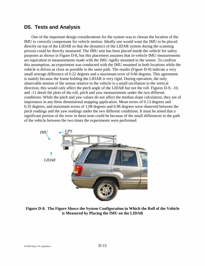
D5. Tests and Analysis
One of the important design considerations for the system was to choose the location of the
IMU to correctly compensate for vehicle motion. Ideally one would want the IMU to be placed
directly on top of the LIDAR so that the dynamics of the LIDAR system during the scanning
process could be directly measured. The IMU unit has been placed inside the vehicle for safety
purposes as shown in Figure D-8, but this placement assumes that in-vehicle IMU measurements
are equivalent to measurements made with the IMU rigidly mounted to the sensor. To confirm
this assumption, an experiment was conducted with the IMU mounted in both locations while the
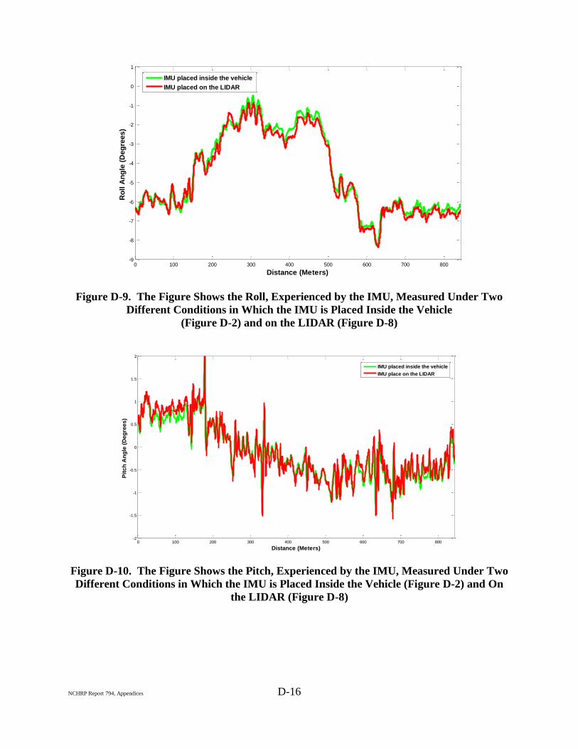
vehicle is driven as close as possible to the same path. The results (Figure D-9) indicate a very
small average difference of 0.22 degrees and a maximum error of 0.66 degrees. This agreement
is mainly because the frame holding the LIDAR is very rigid. During operation, the only
observable motion of the sensor relative to the vehicle is a small oscillation in the vertical
direction; this would only affect the pitch angle of the LIDAR but not the roll. Figures D-9, -10,
and -11 detail the plots of the roll, pitch and yaw measurements under the two different
conditions. While the pitch and yaw values do not affect the median slope calculation, they are of
importance in any three dimensional mapping application. Mean errors of 0.13 degrees and
0.35 degrees, and maximum errors of 1.08 degrees and 0.96 degrees were observed between the
pitch readings and the yaw readings under the two different conditions. It must be noted that a
significant portion of the error in these tests could be because of the small differences in the path
of the vehicle between the two times the experiments were performed.
Figure D-8. The Figure Shows the System Configuration in Which the Roll of the Vehicle
is Measured by Placing the IMU on the LIDAR
LIDAR
IMU
ante
nna
GPS
ante
nna
NCHRP Report 794, Appendices D-16
Figure D-9. The Figure Shows the Roll, Experienced by the IMU, Measured Under Two
Different Conditions in Which the IMU is Placed Inside the Vehicle
(Figure D-2) and on the LIDAR (Figure D-8)
Figure D-10. The Figure Shows the Pitch, Experienced by the IMU, Measured Under Two
Different Conditions in Which the IMU is Placed Inside the Vehicle (Figure D-2) and On
the LIDAR (Figure D-8)
0 100 200 300 400 500 600 700 800-9
-8
-7
-6
-5
-4
-3
-2
-1
0
1
Distance (Meters)
Ro
ll A
ng
le (
Deg
rees)
IMU placed inside the vehicle
IMU placed on the LIDAR
0 100 200 300 400 500 600 700 800-2
-1.5
-1
-0.5
0
0.5
1
1.5
2
Distance (Meters)
Pit
ch
An
gle
(D
eg
rees)
IMU placed inside the vehicle
IMU place on the LIDAR
NCHRP Report 794, Appendices D-17
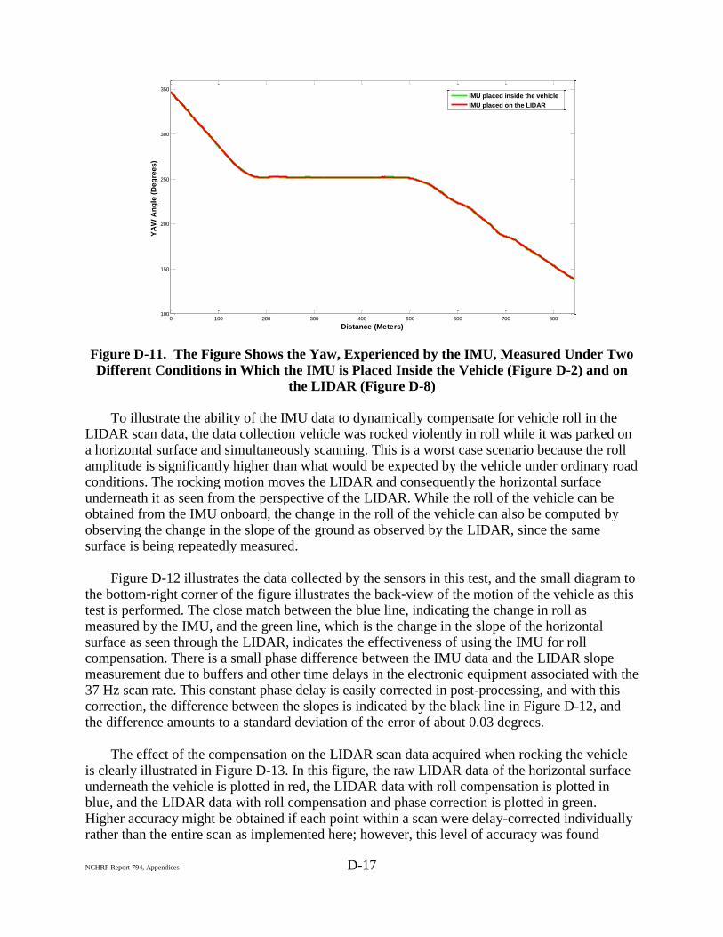
Figure D-11. The Figure Shows the Yaw, Experienced by the IMU, Measured Under Two
Different Conditions in Which the IMU is Placed Inside the Vehicle (Figure D-2) and on
the LIDAR (Figure D-8)
To illustrate the ability of the IMU data to dynamically compensate for vehicle roll in the LIDAR scan data, the data collection vehicle was rocked violently in roll while it was parked on a horizontal surface and simultaneously scanning. This is a worst case scenario because the roll amplitude is significantly higher than what would be expected by the vehicle under ordinary road conditions. The rocking motion moves the LIDAR and consequently the horizontal surface underneath it as seen from the perspective of the LIDAR. While the roll of the vehicle can be obtained from the IMU onboard, the change in the roll of the vehicle can also be computed by observing the change in the slope of the ground as observed by the LIDAR, since the same surface is being repeatedly measured.
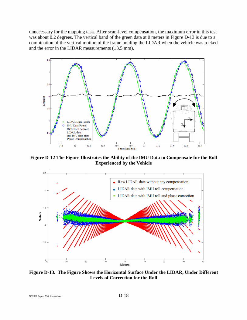
Figure D-12 illustrates the data collected by the sensors in this test, and the small diagram to
the bottom-right corner of the figure illustrates the back-view of the motion of the vehicle as this test is performed. The close match between the blue line, indicating the change in roll as measured by the IMU, and the green line, which is the change in the slope of the horizontal surface as seen through the LIDAR, indicates the effectiveness of using the IMU for roll compensation. There is a small phase difference between the IMU data and the LIDAR slope measurement due to buffers and other time delays in the electronic equipment associated with the 37 Hz scan rate. This constant phase delay is easily corrected in post-processing, and with this correction, the difference between the slopes is indicated by the black line in Figure D-12, and the difference amounts to a standard deviation of the error of about 0.03 degrees.
The effect of the compensation on the LIDAR scan data acquired when rocking the vehicle
is clearly illustrated in Figure D-13. In this figure, the raw LIDAR data of the horizontal surface underneath the vehicle is plotted in red, the LIDAR data with roll compensation is plotted in blue, and the LIDAR data with roll compensation and phase correction is plotted in green. Higher accuracy might be obtained if each point within a scan were delay-corrected individually rather than the entire scan as implemented here; however, this level of accuracy was found
0 100 200 300 400 500 600 700 800100
150
200
250
300
350
Distance (Meters)
YA
W A
ng
le (
De
gre
es)
IMU placed inside the vehicle
IMU placed on the LIDAR
NCHRP Report 794, Appendices D-18
unnecessary for the mapping task. After scan-level compensation, the maximum error in this test was about 0.2 degrees. The vertical band of the green data at 0 meters in Figure D-13 is due to a combination of the vertical motion of the frame holding the LIDAR when the vehicle was rocked and the error in the LIDAR measurements (±3.5 mm).
Figure D-12 The Figure Illustrates the Ability of the IMU Data to Compensate for the Roll
Experienced by the Vehicle
Figure D-13. The Figure Shows the Horizontal Surface Under the LIDAR, Under Different
Levels of Correction for the Roll
y
z
NCHRP Report 794, Appendices D-19
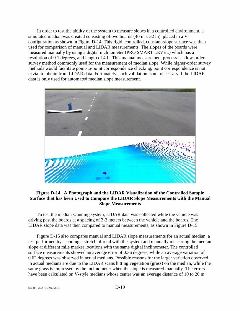
In order to test the ability of the system to measure slopes in a controlled environment, a
simulated median was created consisting of two boards (40 in × 32 in) placed in a V
configuration as shown in Figure D-14. This rigid, controlled, constant-slope surface was then used for comparison of manual and LIDAR measurements. The slopes of the boards were measured manually by using a digital inclinometer (PRO SMART LEVEL) which has a resolution of 0.1 degrees, and length of 4 ft. This manual measurement process is a low-order survey method commonly used for the measurement of median slope. While higher-order survey methods would facilitate point-to-point correspondence checking, point correspondence is not trivial to obtain from LIDAR data. Fortunately, such validation is not necessary if the LIDAR data is only used for automated median slope measurement.
Figure D-14. A Photograph and the LIDAR Visualization of the Controlled Sample
Surface that has been Used to Compare the LIDAR Slope Measurements with the Manual
Slope Measurements
To test the median scanning system, LIDAR data was collected while the vehicle was
driving past the boards at a spacing of 2-3 meters between the vehicle and the boards. The
LIDAR slope data was then compared to manual measurements, as shown in Figure D-15.
Figure D-15 also compares manual and LIDAR slope measurements for an actual median, a
test performed by scanning a stretch of road with the system and manually measuring the median
slope at different mile marker locations with the same digital inclinometer. The controlled
surface measurements showed an average error of 0.36 degrees, while an average variation of
0.62 degrees was observed in actual medians. Possible reasons for the larger variation observed
in actual medians are due to the LIDAR scans hitting vegetation (grass) on the median, while the
same grass is impressed by the inclinometer when the slope is measured manually. The errors
have been calculated on V-style medians whose center was an average distance of 10 to 20 m
NCHRP Report 794, Appendices D-20
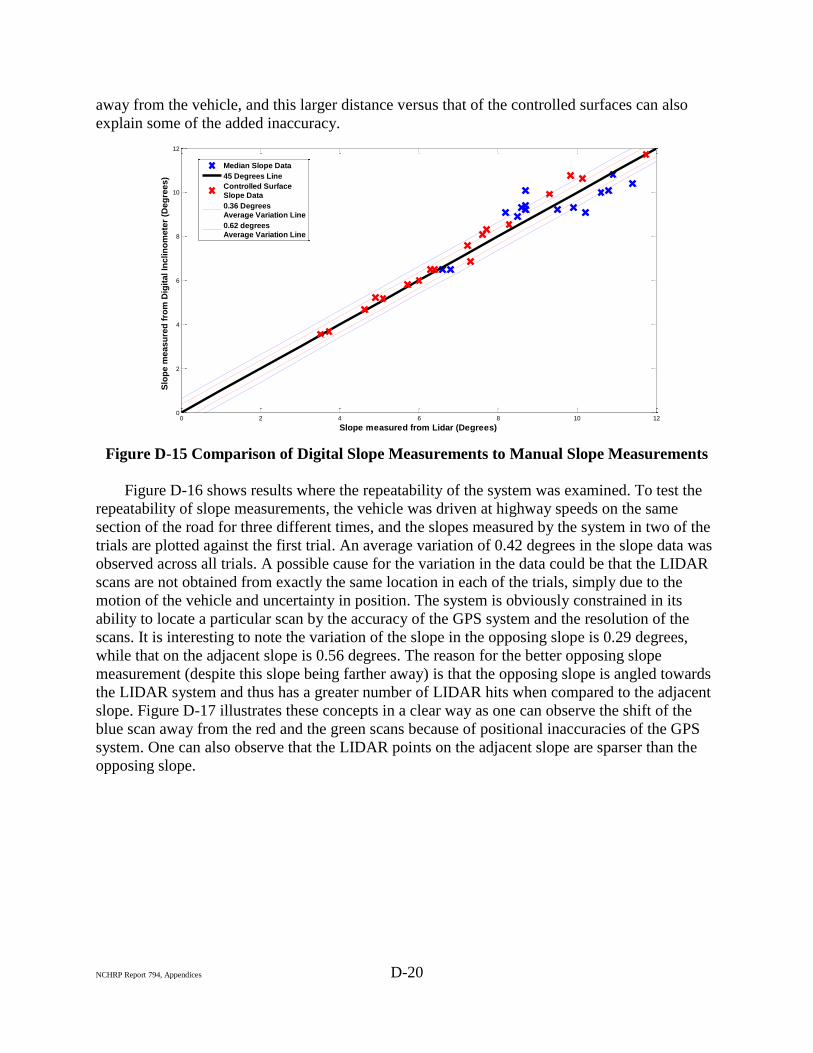
away from the vehicle, and this larger distance versus that of the controlled surfaces can also
explain some of the added inaccuracy.
Figure D-15 Comparison of Digital Slope Measurements to Manual Slope Measurements
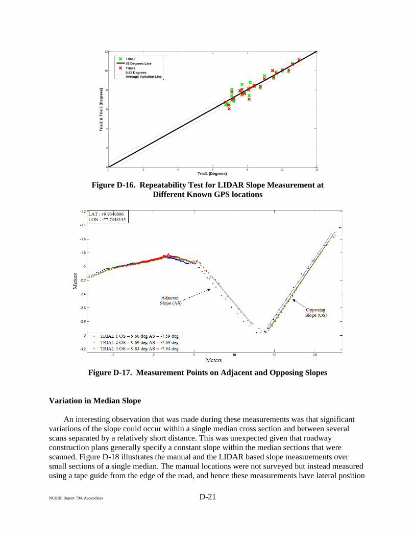
Figure D-16 shows results where the repeatability of the system was examined. To test the
repeatability of slope measurements, the vehicle was driven at highway speeds on the same
section of the road for three different times, and the slopes measured by the system in two of the
trials are plotted against the first trial. An average variation of 0.42 degrees in the slope data was
observed across all trials. A possible cause for the variation in the data could be that the LIDAR
scans are not obtained from exactly the same location in each of the trials, simply due to the
motion of the vehicle and uncertainty in position. The system is obviously constrained in its
ability to locate a particular scan by the accuracy of the GPS system and the resolution of the
scans. It is interesting to note the variation of the slope in the opposing slope is 0.29 degrees,
while that on the adjacent slope is 0.56 degrees. The reason for the better opposing slope
measurement (despite this slope being farther away) is that the opposing slope is angled towards
the LIDAR system and thus has a greater number of LIDAR hits when compared to the adjacent
slope. Figure D-17 illustrates these concepts in a clear way as one can observe the shift of the
blue scan away from the red and the green scans because of positional inaccuracies of the GPS
system. One can also observe that the LIDAR points on the adjacent slope are sparser than the
opposing slope.
0 2 4 6 8 10 120
2
4
6
8
10
12
Slope measured from Lidar (Degrees)
Slo
pe
me
as
ure
d f
rom
Dig
ital
Incli
no
mete
r (D
eg
ree
s)
Median Slope Data
45 Degrees Line
Controlled Surface
Slope Data
0.36 Degrees
Average Variation Line
0.62 degrees
Average Variation Line
NCHRP Report 794, Appendices D-21
Figure D-16. Repeatability Test for LIDAR Slope Measurement at
Different Known GPS locations
Figure D-17. Measurement Points on Adjacent and Opposing Slopes
Variation in Median Slope
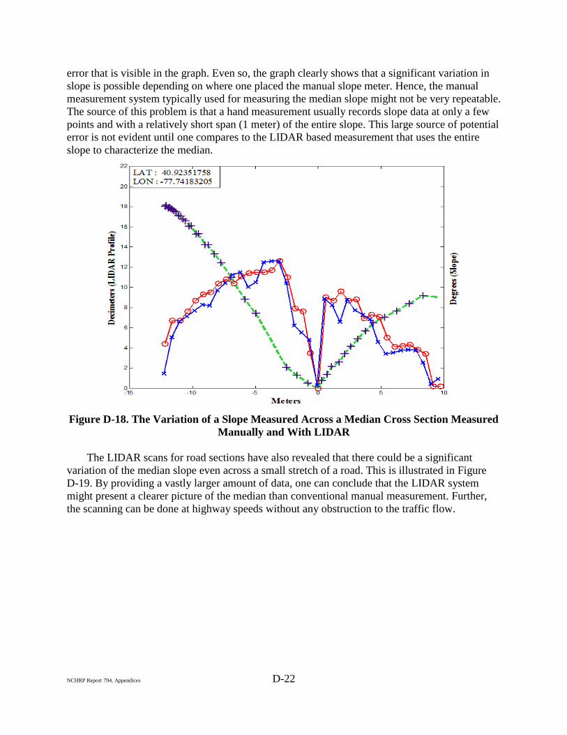
An interesting observation that was made during these measurements was that significant
variations of the slope could occur within a single median cross section and between several
scans separated by a relatively short distance. This was unexpected given that roadway
construction plans generally specify a constant slope within the median sections that were
scanned. Figure D-18 illustrates the manual and the LIDAR based slope measurements over
small sections of a single median. The manual locations were not surveyed but instead measured
using a tape guide from the edge of the road, and hence these measurements have lateral position
0 2 4 6 8 10 120
2
4
6
8
10
12
Trial1 (Degrees)
Tri
al2
& T
rial3
(D
eg
rees)
Trial 2
45 Degrees Line
Trial 3
0.42 Degrees
Average Variation Line
NCHRP Report 794, Appendices D-22
error that is visible in the graph. Even so, the graph clearly shows that a significant variation in
slope is possible depending on where one placed the manual slope meter. Hence, the manual
measurement system typically used for measuring the median slope might not be very repeatable.
The source of this problem is that a hand measurement usually records slope data at only a few
points and with a relatively short span (1 meter) of the entire slope. This large source of potential
error is not evident until one compares to the LIDAR based measurement that uses the entire
slope to characterize the median.
Figure D-18. The Variation of a Slope Measured Across a Median Cross Section Measured
Manually and With LIDAR
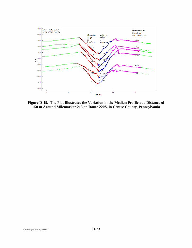
The LIDAR scans for road sections have also revealed that there could be a significant
variation of the median slope even across a small stretch of a road. This is illustrated in Figure
D-19. By providing a vastly larger amount of data, one can conclude that the LIDAR system
might present a clearer picture of the median than conventional manual measurement. Further,
the scanning can be done at highway speeds without any obstruction to the traffic flow.
NCHRP Report 794, Appendices D-23
Figure D-19. The Plot Illustrates the Variation in the Median Profile at a Distance of
±50 m Around Milemarker 213 on Route 220S, in Centre County, Pennsylvania
NCHRP Report 794, Appendices D-24
NCHRP Report 794, Appendices D-25
D6. Conclusions and Future Work
This appendix presents a LIDAR-based scanning technology for measuring the median slope
and compares it to manual measurement techniques. The results indicate accuracies on the order
of 0.36 degrees in controlled tests with fixed surfaces, and 0.62 degrees for tests on actual
medians. Repeatability was found to be approximately 0.42 degrees for actual median scans. The
compensation of vehicle motion was found to be quite good, and independent of whether the
IMU was mounted on the LIDAR sensor or mounted within the vehicle. Using tests where the
vehicle was aggressively rocked back and forth, the error due to compensation for vehicle
motion was found to be 0.03 degrees.
The system is very cost effective with an approximate expense of $1/mi (2,250 data
points/mile/minute) to take measurements as compared to manual measurement which has been
estimated to cost $100/mile (5 data points/mi/100 min), an estimate from past work by
researchers at Penn State. This 100 times cost savings agrees with estimates from other
researchers. (22)
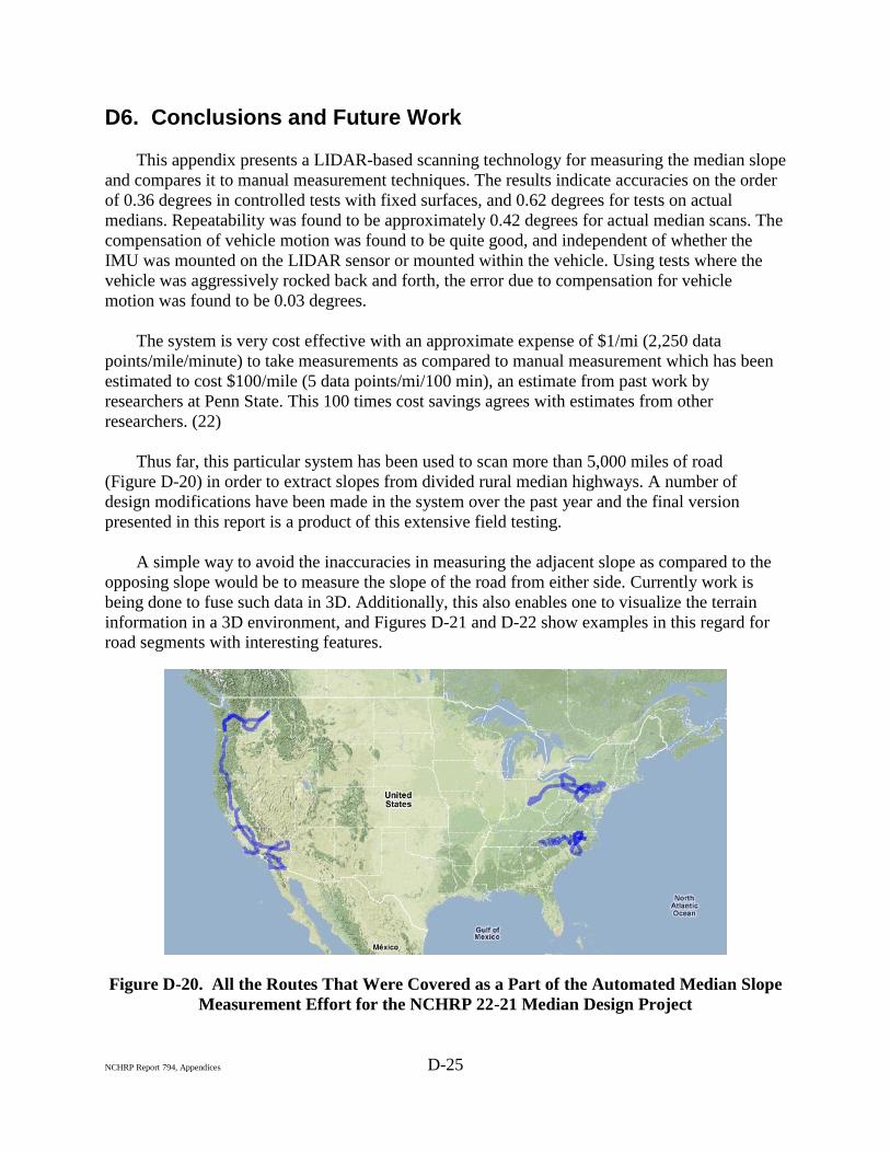
Thus far, this particular system has been used to scan more than 5,000 miles of road
(Figure D-20) in order to extract slopes from divided rural median highways. A number of
design modifications have been made in the system over the past year and the final version
presented in this report is a product of this extensive field testing.
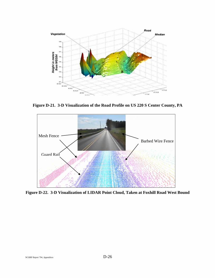
A simple way to avoid the inaccuracies in measuring the adjacent slope as compared to the
opposing slope would be to measure the slope of the road from either side. Currently work is
being done to fuse such data in 3D. Additionally, this also enables one to visualize the terrain
information in a 3D environment, and Figures D-21 and D-22 show examples in this regard for
road segments with interesting features.
Figure D-20. All the Routes That Were Covered as a Part of the Automated Median Slope
Measurement Effort for the NCHRP 22-21 Median Design Project
NCHRP Report 794, Appendices D-26
Figure D-21. 3-D Visualization of the Road Profile on US 220 S Center County, PA
Figure D-22. 3-D Visualization of LIDAR Point Cloud, Taken at Foxhill Road West Bound
Guard Rail
Mesh Fence
Barbed Wire Fence
NCHRP Report 794, Appendices 27
Appendix E
Economic Analyses
NCHRP Report 794, Appendices 28
NCHRP Report 794, Appendices E-1
This appendix addresses the types of economic analysis performed in the research.
E.1 Overview
Several types of economic analyses have been conducted to examine issues related to median cross-section design. The issues addressed include:
safety benefit analysis for wider medians benefit-cost analysis for flatter median slopes benefit-cost analysis for installation of median barriers
All of the economic analyses address rural four-lane freeways. The economic analyses were
conducted to help interpret the results of the crash analyses presented in Section 4 of this report. However, these economic analyses do not reflect the full research results, because they do not incorporate the results of the vehicle dynamics simulation analyses presented in Section 5, which form a key part of the design recommendations. The vehicle dynamics simulation results are, by their nature, not suitable for consideration in an economic analysis. Therefore, these economic analysis results should be interpreted cautiously, as they are not sufficiently complete to serve as a geometric design tool or as a median barrier selection tool.
E.2 Crash Costs
The estimated crash costs used in the economic analysis are based on those used in SafetyAnalyst (64), which are based on the most recently published FHWA values (65):
Fatal crash $5,800,000 A injury crash 402,000 B injury crash 80,000 C injury crash 42,000 Property-damage-only crash 4,000
The weighted average cost for an injury crash (for all nonfatal injury severity levels
combined, assuming 4.8 percent A injuries, 25.7 percent B injuries, and 69.5 percent C injuries, based on Washington data for rural freeways) is $69,000. The combined weighted-average cost for fatal-and-injury crashes is $527,480 for crashes related to traversable medians and $321,160 for crashes related to barrier medians, based on the proportions of fatal crashes and injury crashes shown in Table 64.
E.3 Safety Benefit Analysis for Wider Medians
The crash analyses in Section 4 of this report show that, for rural four-lane freeways, wider medians reduce CMC crashes, but increase rollover crashes. These effects are represented by the model coefficients presented in Tables 34 and 35 that apply to median width for total crashes and
NCHRP Report 794, Appendices E-2
fatal-and-injury crashes, respectively. The median width coefficients for fatal-and-injury crashes from Table 35 are:
–0.0205 crashes/mi/yr per foot of median width for CMC crashes +0.0216 crashes/mi/yr per foot of median width for rollover crashes
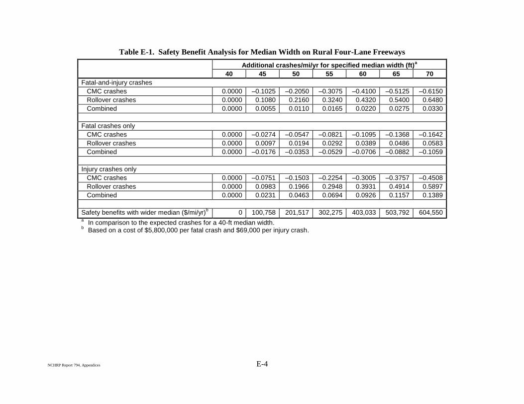
Table E-1 shows the decreased CMC crashes and increased rollover crashes that would
occur each year in a 1.6 km (1-mi) length of median for 1.5-m (5-ft) increments of increasing median width from the base condition of a 12-m (40-ft) median width. The top portion of the table provides an estimate for additional fatal-and-injury crashes by crash type based on the model coefficients shown above. The additional crashes are then broken down into separate estimates of fatal and injury crashes based on the crash proportions shown in Table 64. Specifically, for traversable medians on rural four-lane freeways, fatal crashes constitute 26.7 percent of fatal-and-injury CMC crashes, but only 9.0 percent of fatal-and-injury rollover crashes.
The results in Table E-1 show that, as the median gets wider, fatal crash frequency decreases, while injury crash frequency increases. The final line in the table shows the annual safety benefits for each median width, in comparison to a 12-m (40-ft) median, based on the crash costs presented in Section E.1 of this appendix. The results show that wider medians produce consistently larger safety benefits. The discussion in Section 6 of this report shows that there are probably limits to this trend that are evident in the vehicle dynamics simulation analysis, but not in the crash analysis.
No benefit-cost analysis was conducted for median width because the grading costs for providing wider medians vary widely. However, it is likely that the safety benefits shown in Table E-1 would make wider medians cost-effective as part of new construction, but not necessarily in reconstruction projects.
E.4 Cost-Benefit Analysis for Flatter Median Slopes
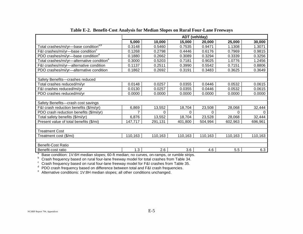
Table E-2 shows the results of a benefit-cost analysis for median slopes on rural four-lane freeways. Specifically, the analysis focuses on the selection of either 1V:6H or 1V:8H median slopes.
The base condition for the analysis is a 60-ft median with 1V:6H median slopes on a rural four-lane freeway section with no horizontal curves, no on-ramps, and no rumble strips. Crash frequencies for the base condition are based on the rural four-lane freeway models for total median-related crashes in Table 34 and for F&I median-related crashes in Table 35. Crash frequencies are shown for freeway sections with traffic volumes ranging from 5,000 to 30,000 veh/day.
The alternative condition for the analysis is based on an identical freeway section with 1V:8H median slopes, rather than 1V:6H median slopes. The crash frequencies for this condition are estimated with the same models as for the base condition.
NCHRP Report 794, Appendices E-3
The frequency of crashes reduced is based on the difference between the crash frequencies for the base and alternative conditions. The crash reduction benefits are crash cost savings based on the crash costs presented in Section E.1. The present value of the benefits is determined with the uniform series present worth factor based on an expected service life of 50 years for a rural freeway median and a minimum attractive rate of return (discount rate) of 4 percent, representing the real long-term cost of capital.
NCHRP Report 794, Appendices E-4
Table E-1. Safety Benefit Analysis for Median Width on Rural Four-Lane Freeways
Additional crashes/mi/yr for specified median width (ft)a
Benefit-cost ratio 4.2 4.3 4.5 4.7 4.8 14.7 15.3 15.8 16.4 16.9 a Based on F&I crashes model for all median-related crashes on rural four-lane freeways in Table 35; break down by crash type based on Table 30.
b Breakdown of F&I crashes into separate fatal and injury crash frequencies based on crash severity proportions for traversable medians in Table 64.
c F&I crashes for barrier medians based on F&I crashes for traversable medians multiplied by crash reduction factors for flexible medians from before-after evaluation
results in Table 59. d Breakdown of F&I crashes into separate fatal and injury crash frequencies based on crash severity proportions for barrier medians in Table 64.
e Based on $5,800,000 per fatal crash reduced and $69,000 per injury reduced (see Section E.1).
NCHRP Report 794--Appendices.doc E-10
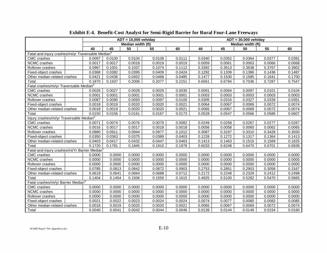
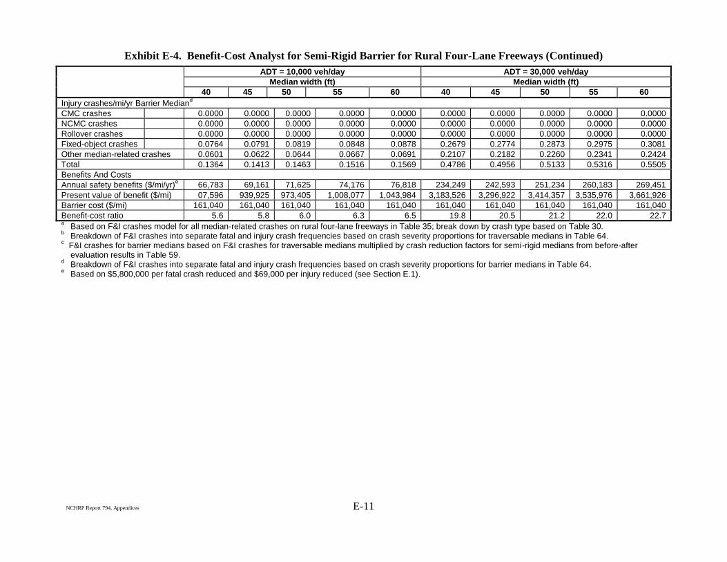
Exhibit E-4. Benefit-Cost Analyst for Semi-Rigid Barrier for Rural Four-Lane Freeways
Benefit-cost ratio 5.6 5.8 6.0 6.3 6.5 19.8 20.5 21.2 22.0 22.7 a Based on F&I crashes model for all median-related crashes on rural four-lane freeways in Table 35; break down by crash type based on Table 30.
b Breakdown of F&I crashes into separate fatal and injury crash frequencies based on crash severity proportions for traversable medians in Table 64.
c F&I crashes for barrier medians based on F&I crashes for traversable medians multiplied by crash reduction factors for semi-rigid medians from before-after
evaluation results in Table 59. d Breakdown of F&I crashes into separate fatal and injury crash frequencies based on crash severity proportions for barrier medians in Table 64.
e Based on $5,800,000 per fatal crash reduced and $69,000 per injury reduced (see Section E.1).
NCHRP Report 794, Appendices E-12
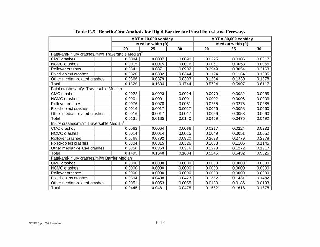
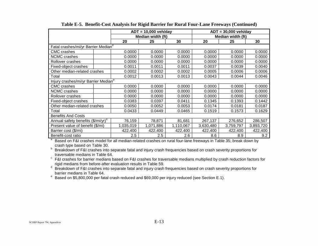
Table E-5. Benefit-Cost Analysis for Rigid Barrier for Rural Four-Lane Freeways
Benefit-cost ratio 2.5 2.5 2.6 8.6 8.9 9.2 a Based on F&I crashes model for all median-related crashes on rural four-lane freeways in Table 35; break down by
crash type based on Table 30. b Breakdown of F&I crashes into separate fatal and injury crash frequencies based on crash severity proportions for
traversable medians in Table 64. c F&I crashes for barrier medians based on F&I crashes for traversable medians multiplied by crash reduction factors for
rigid medians from before-after evaluation results in Table 59. d Breakdown of F&I crashes into separate fatal and injury crash frequencies based on crash severity proportions for
barrier medians in Table 64. e Based on $5,800,000 per fatal crash reduced and $69,000 per injury reduced (see Section E.1).