55
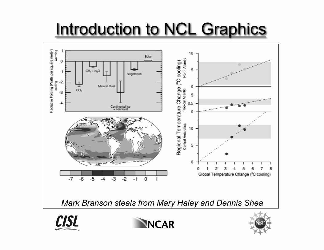
Introduction to NCL Graphics Mark Branson steals from Mary Haley and Dennis Shea
| Date post: | 23-Oct-2015 |
| Category: |
Documents |
| Upload: | surajatmos458 |
| View: | 74 times |
| Download: | 0 times |
Introduction to NCL Graphics
Mark Branson steals from Mary Haley and Dennis Shea
Introduction to NCL Graphics
My goals for this FAPCRD Familiarize you with the structure of an NCL
graphics script Get you started with understanding resources Show you the most common things users need
to do with NCL graphics Show you debugging tips and common user
mistakes Provide you with useful documentation links
Introduction to NCL Graphics
Overview NCL is a product of Computational and
Information Systems Laboratory (CISL) at NCAR, sponsored by NSF
free interpreted language designed specifically for scientific data processing and visualization
robust file input and output: it can read and write netCDF-3, netCDF-4 classic, HDF4, binary and ASCII data. It can read HDF-EOS, GRIB1, GRIB2, etc.

Introduction to NCL Graphics
intended to be an objected-oriented language, but GSN libraries provide a simpler interface (GSN = getting started using NCL).
can be run in interactive mode or batch mode over 600 built-in functions can call C and Fortran external routines fantastic examples on their website, great support
Introduction to NCL Graphics
Topics • Quick tour of high-level graphics interfaces • How to get it working on your Mac • Basic code structure for NCL graphics • Step-by-step NCL visualization examples • Customizing your NCL graphics environment • Debugging tips and common mistakes
Introduction to NCL Graphics
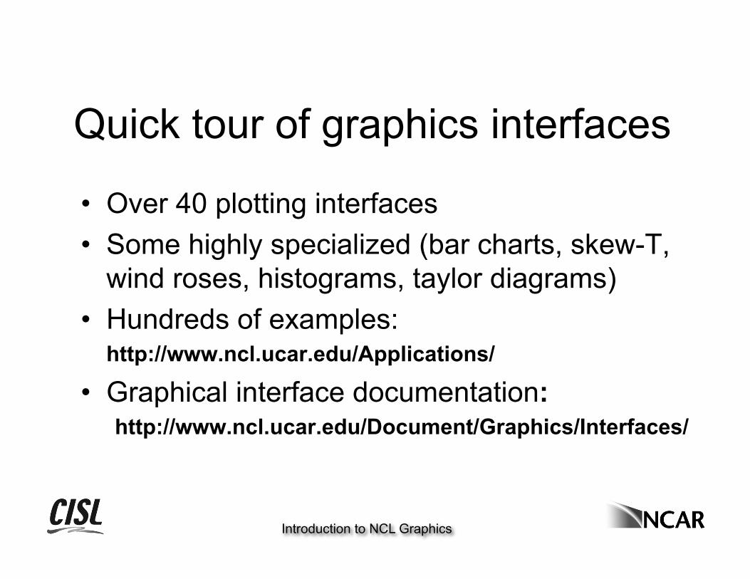
Quick tour of graphics interfaces
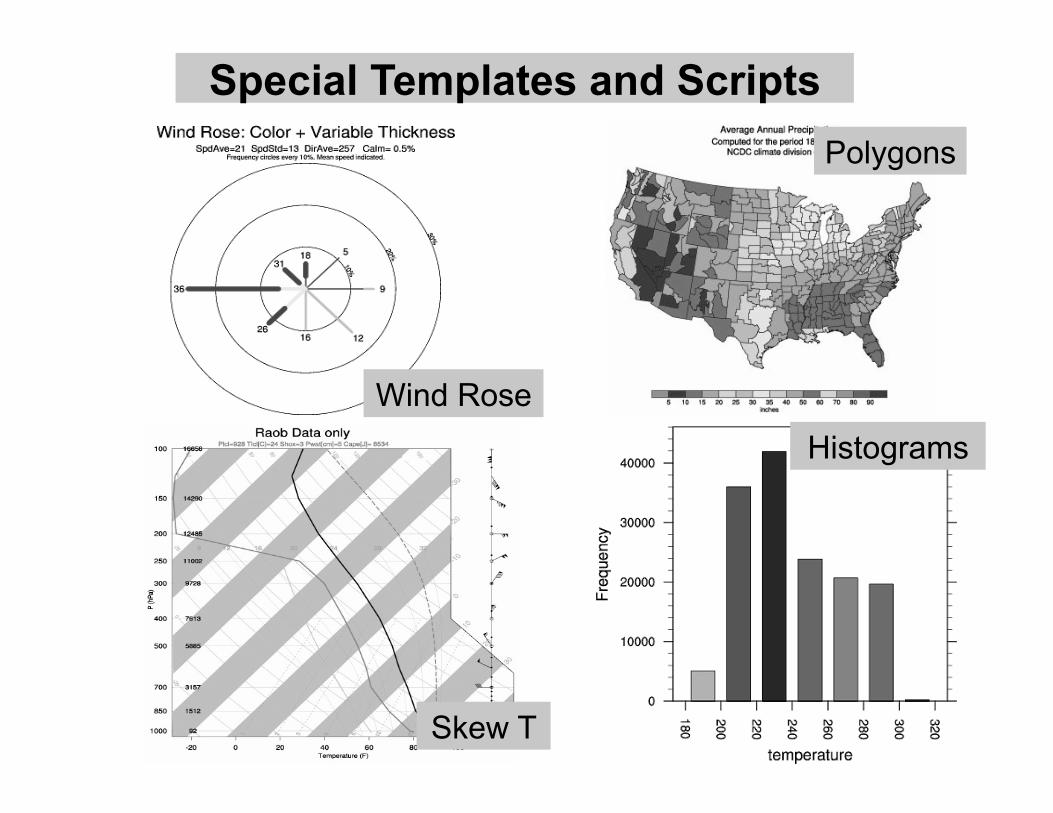
• Over 40 plotting interfaces • Some highly specialized (bar charts, skew-T,
wind roses, histograms, taylor diagrams) • Hundreds of examples:
http://www.ncl.ucar.edu/Applications/
• Graphical interface documentation: http://www.ncl.ucar.edu/Document/Graphics/Interfaces/
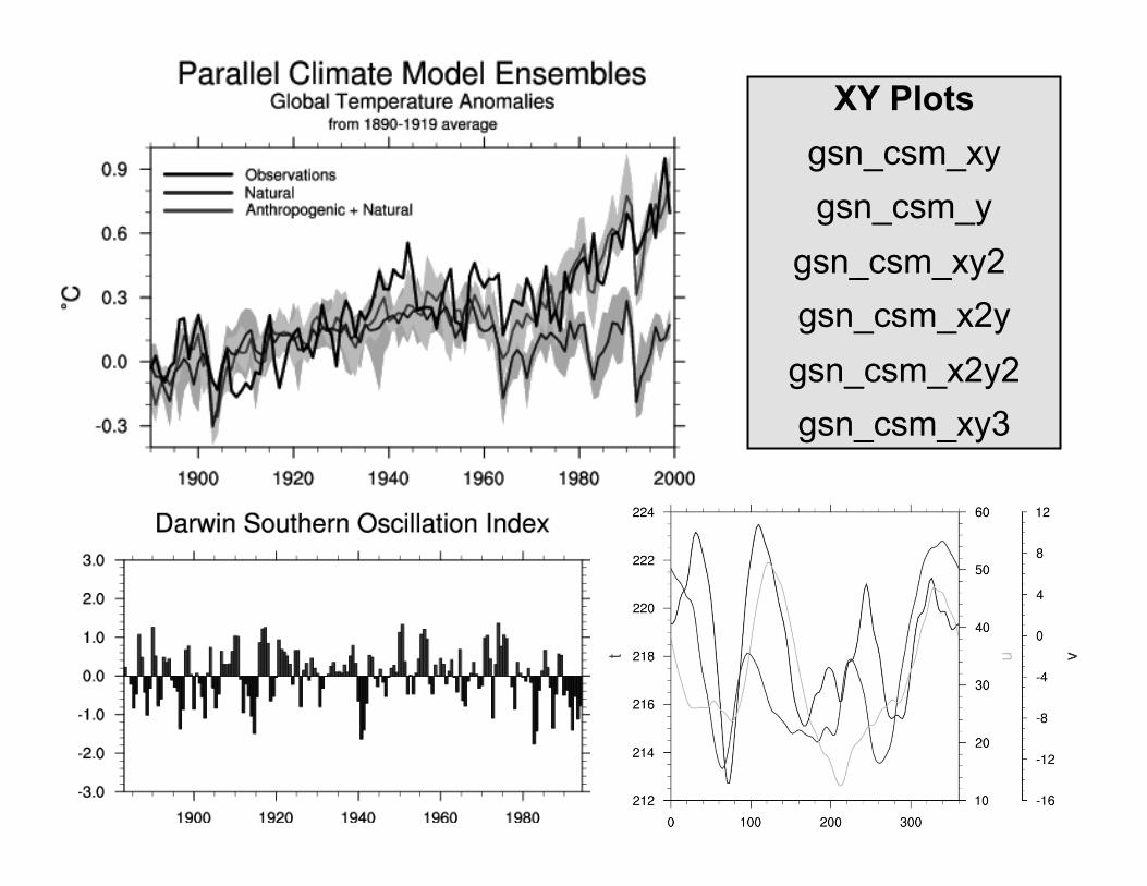
XY Plots gsn_csm_xy gsn_csm_y
gsn_csm_xy2 gsn_csm_x2y
gsn_csm_x2y2 gsn_csm_xy3
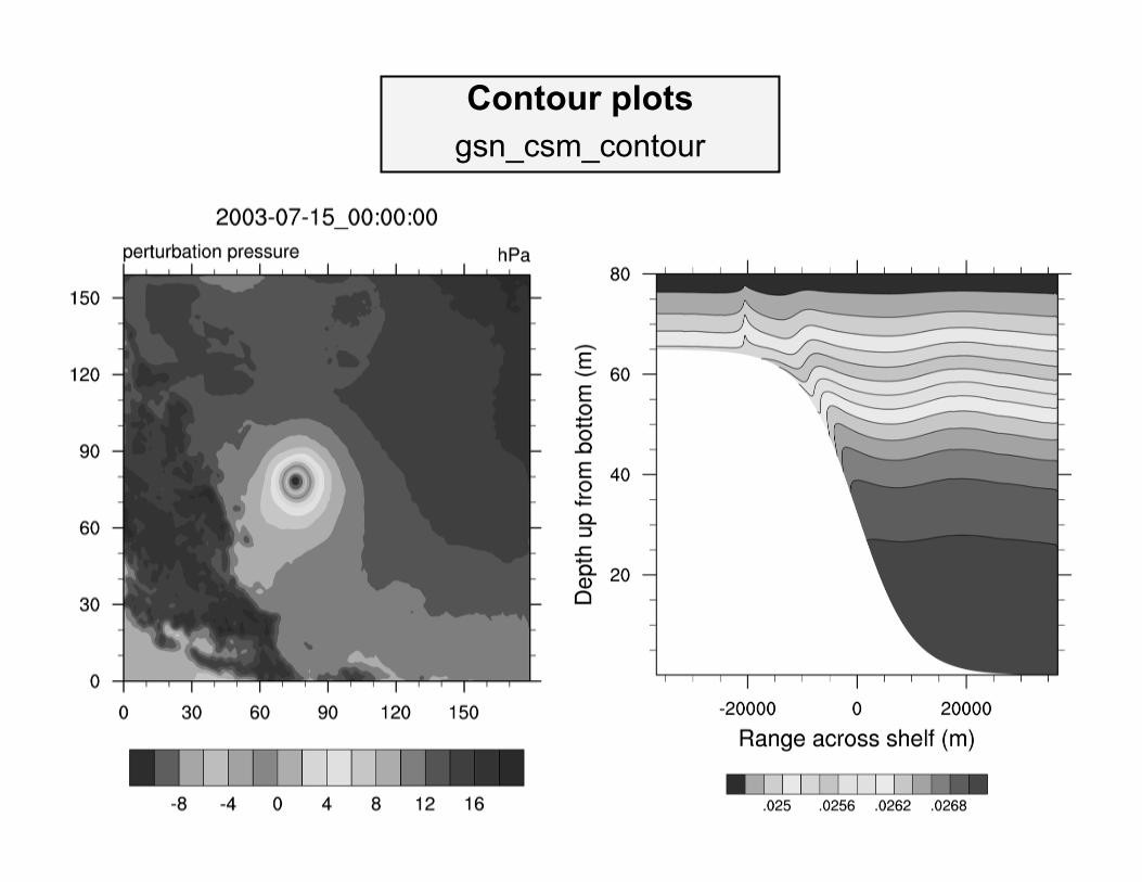
Contour plots gsn_csm_contour
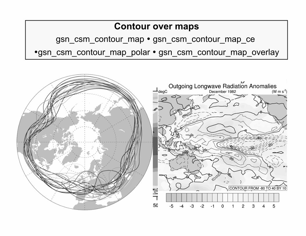
Contour over maps gsn_csm_contour_map • gsn_csm_contour_map_ce
•gsn_csm_contour_map_polar • gsn_csm_contour_map_overlay
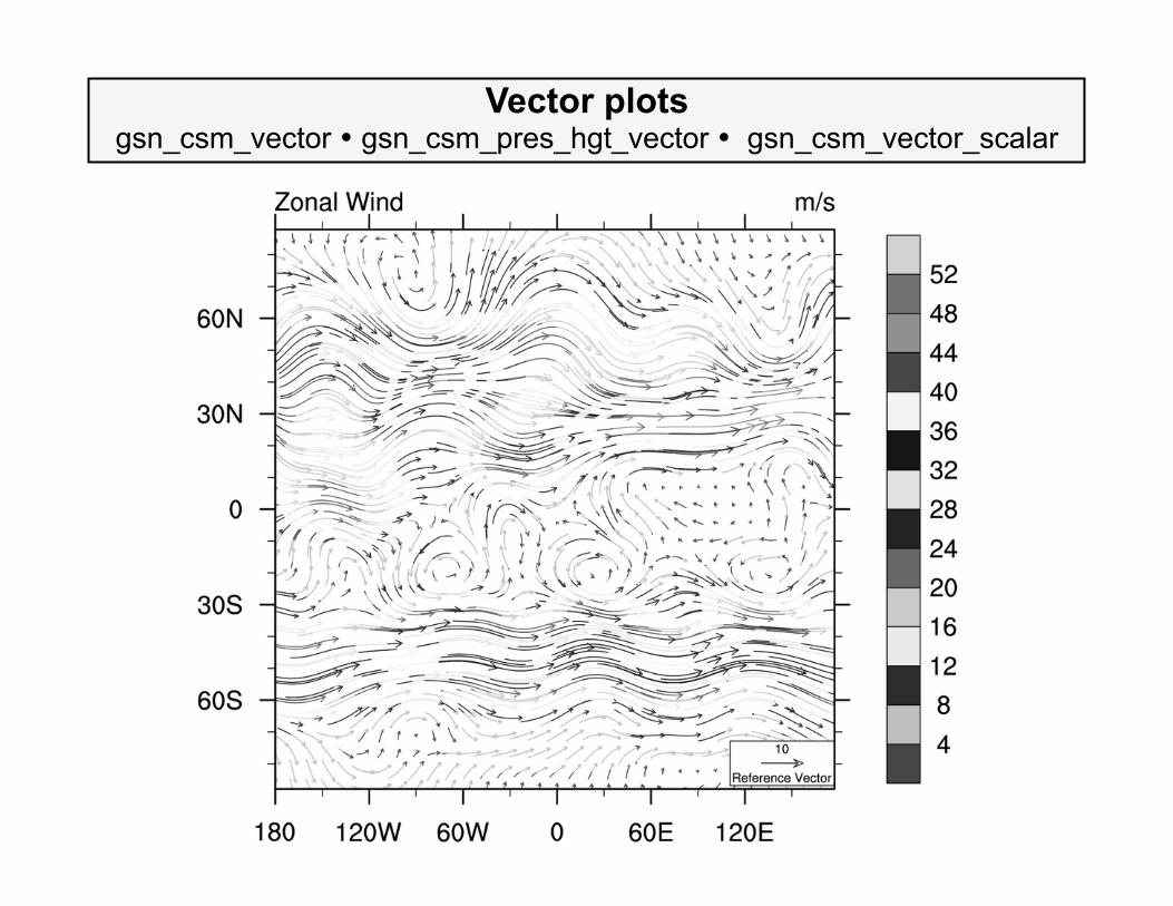
Vector plots gsn_csm_vector • gsn_csm_pres_hgt_vector • gsn_csm_vector_scalar
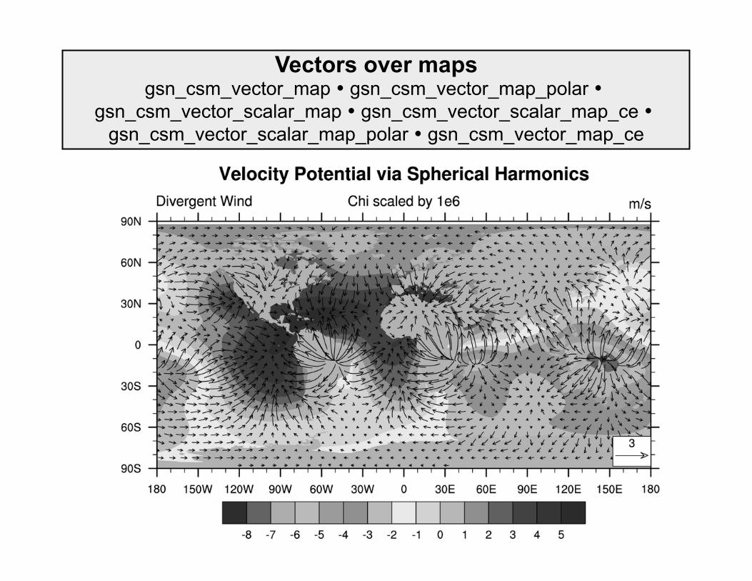
Vectors over maps gsn_csm_vector_map • gsn_csm_vector_map_polar •
gsn_csm_vector_scalar_map • gsn_csm_vector_scalar_map_ce • gsn_csm_vector_scalar_map_polar • gsn_csm_vector_map_ce
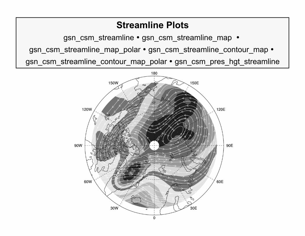
Streamline Plots gsn_csm_streamline • gsn_csm_streamline_map •
gsn_csm_streamline_map_polar • gsn_csm_streamline_contour_map • gsn_csm_streamline_contour_map_polar • gsn_csm_pres_hgt_streamline
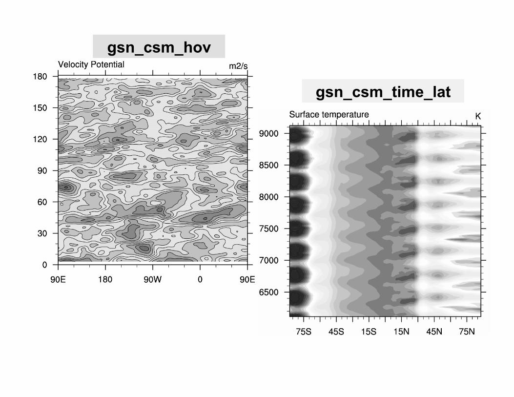
gsn_csm_hov
gsn_csm_time_lat
skew-t.ncl
Special Templates and Scripts
Wind Rose
Polygons
Histograms
Skew T
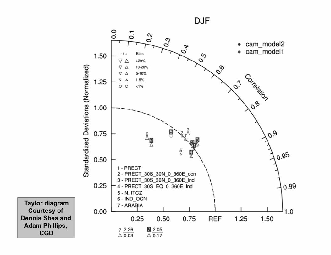
Taylor diagram Courtesy of
Dennis Shea and Adam Phillips,
CGD
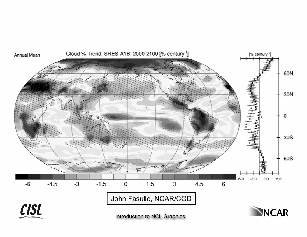
Introduction to NCL Graphics
John Fasullo, NCAR/CGD
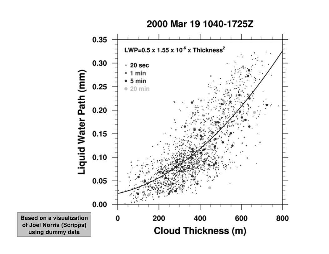
Based on a visualization of Joel Norris (Scripps)
using dummy data
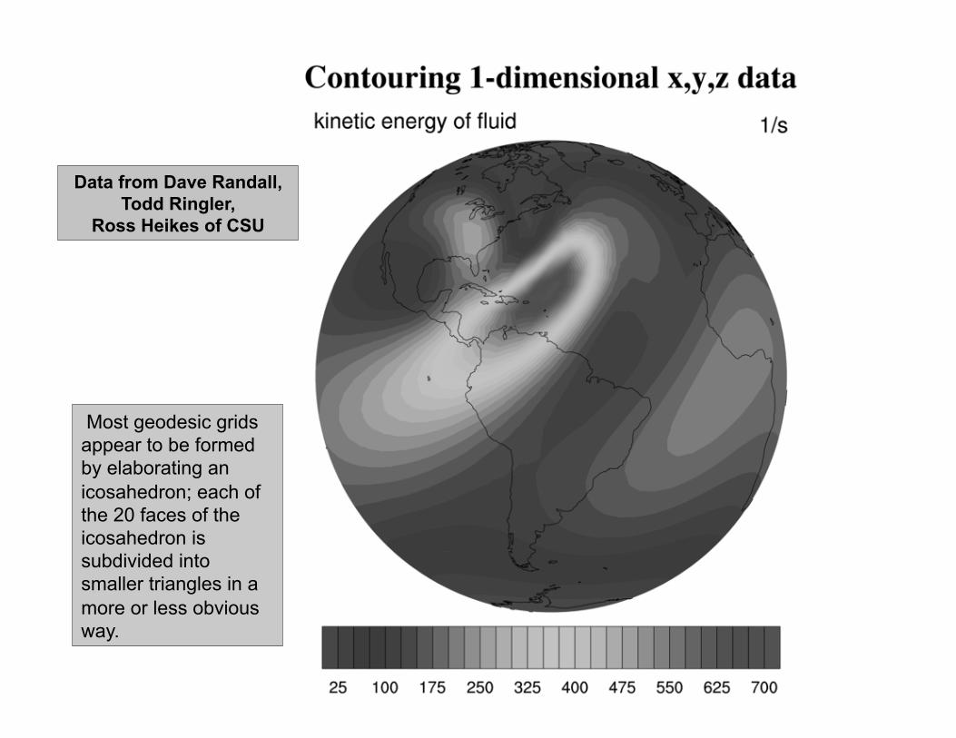
Data from Dave Randall, Todd Ringler,
Ross Heikes of CSU
Most geodesic grids appear to be formed by elaborating an icosahedron; each of the 20 faces of the icosahedron is subdivided into smaller triangles in a more or less obvious way.
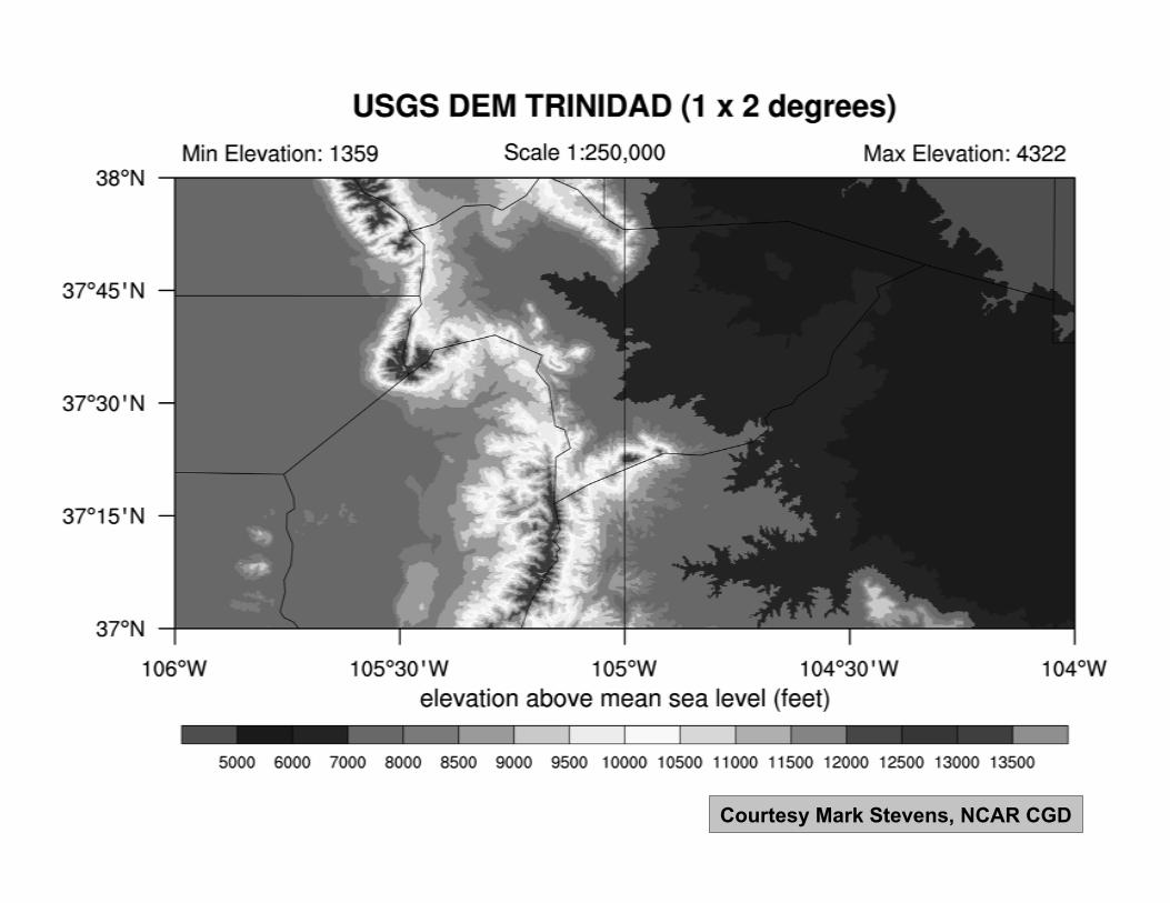
Courtesy Mark Stevens, NCAR CGD
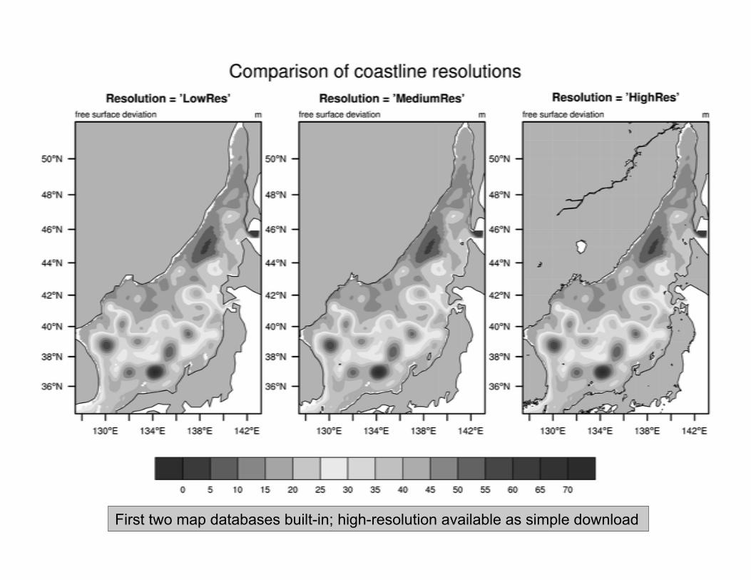
First two map databases built-in; high-resolution available as simple download
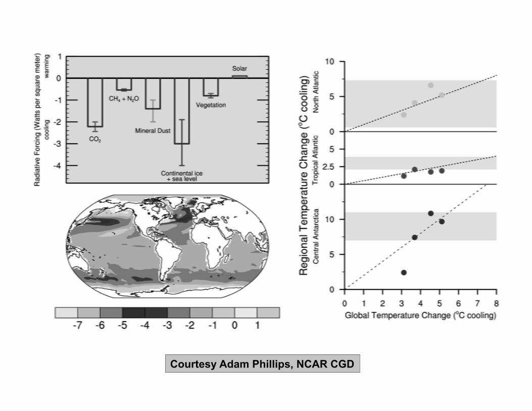
Courtesy Adam Phillips, NCAR CGD
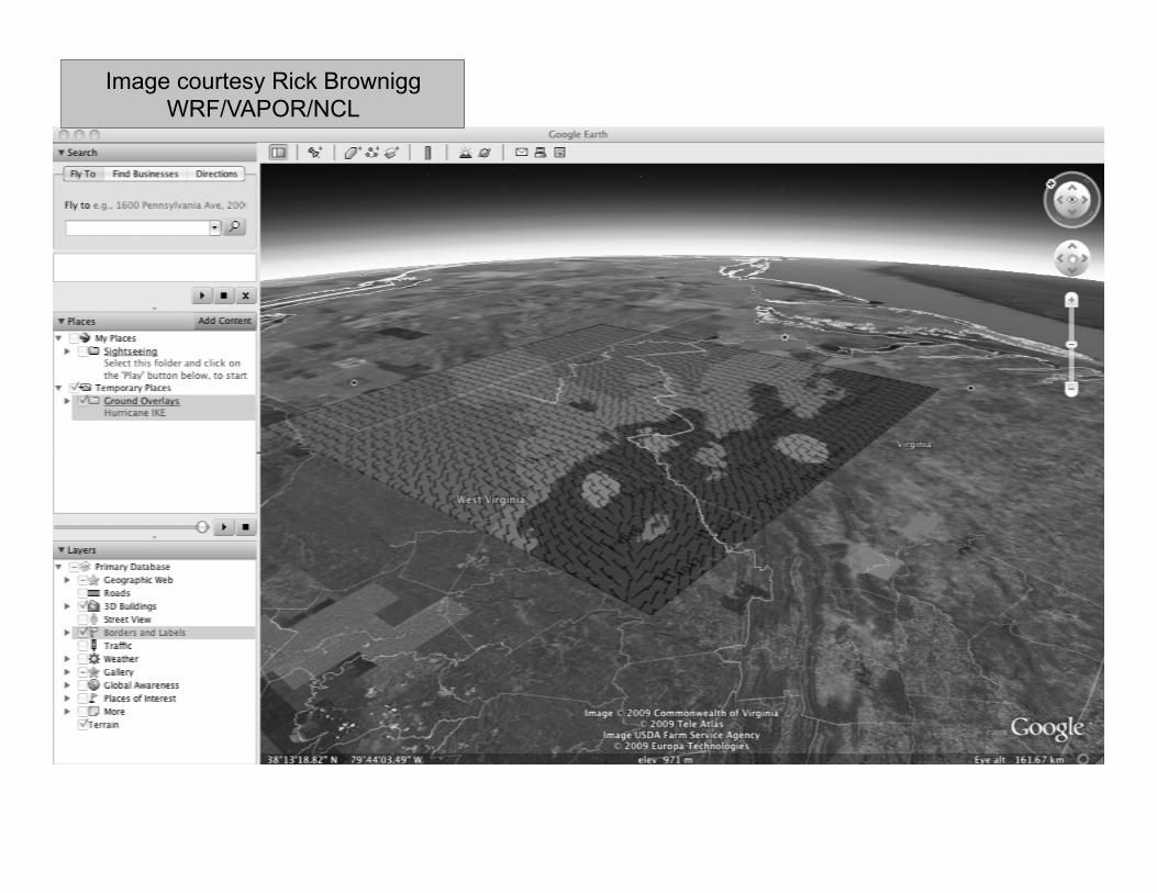
Image courtesy Rick Brownigg WRF/VAPOR/NCL
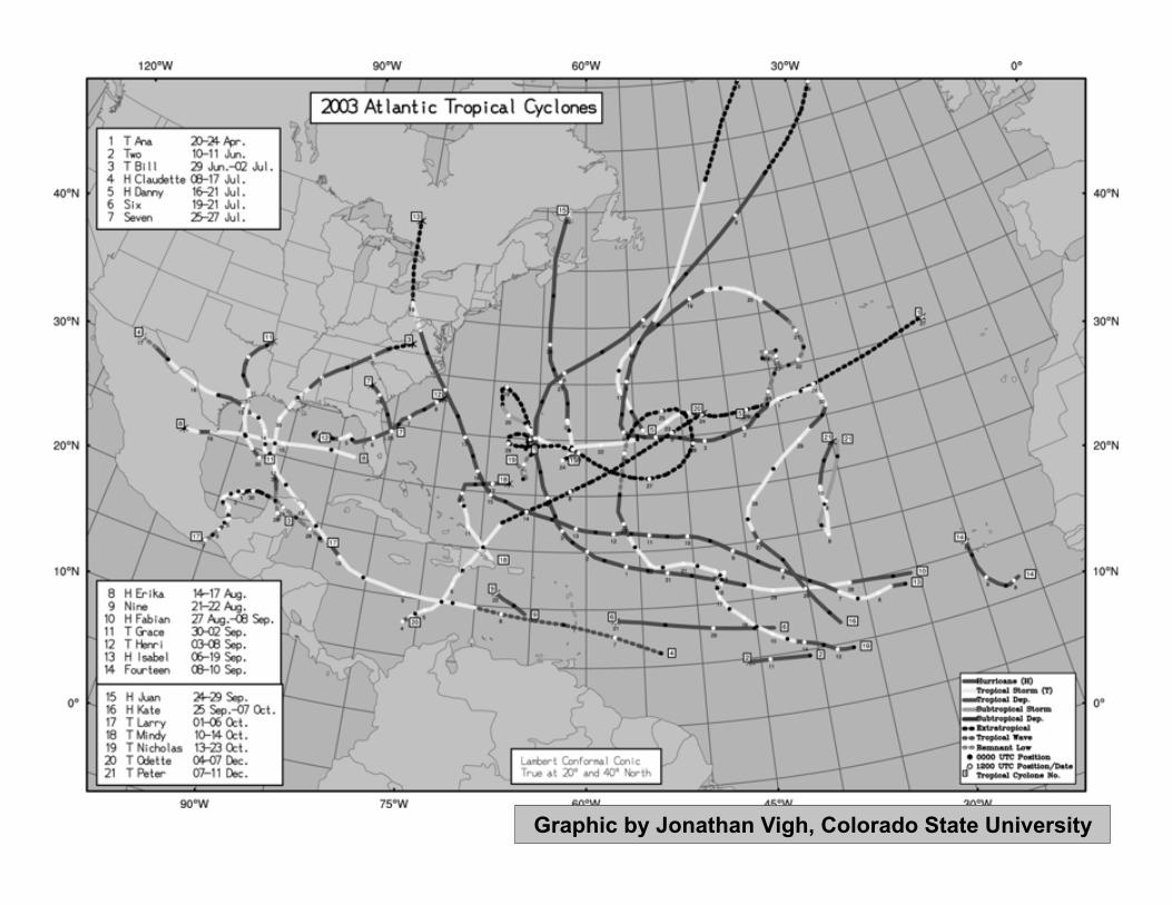
Graphic by Jonathan Vigh, Colorado State University
Introduction to NCL Graphics
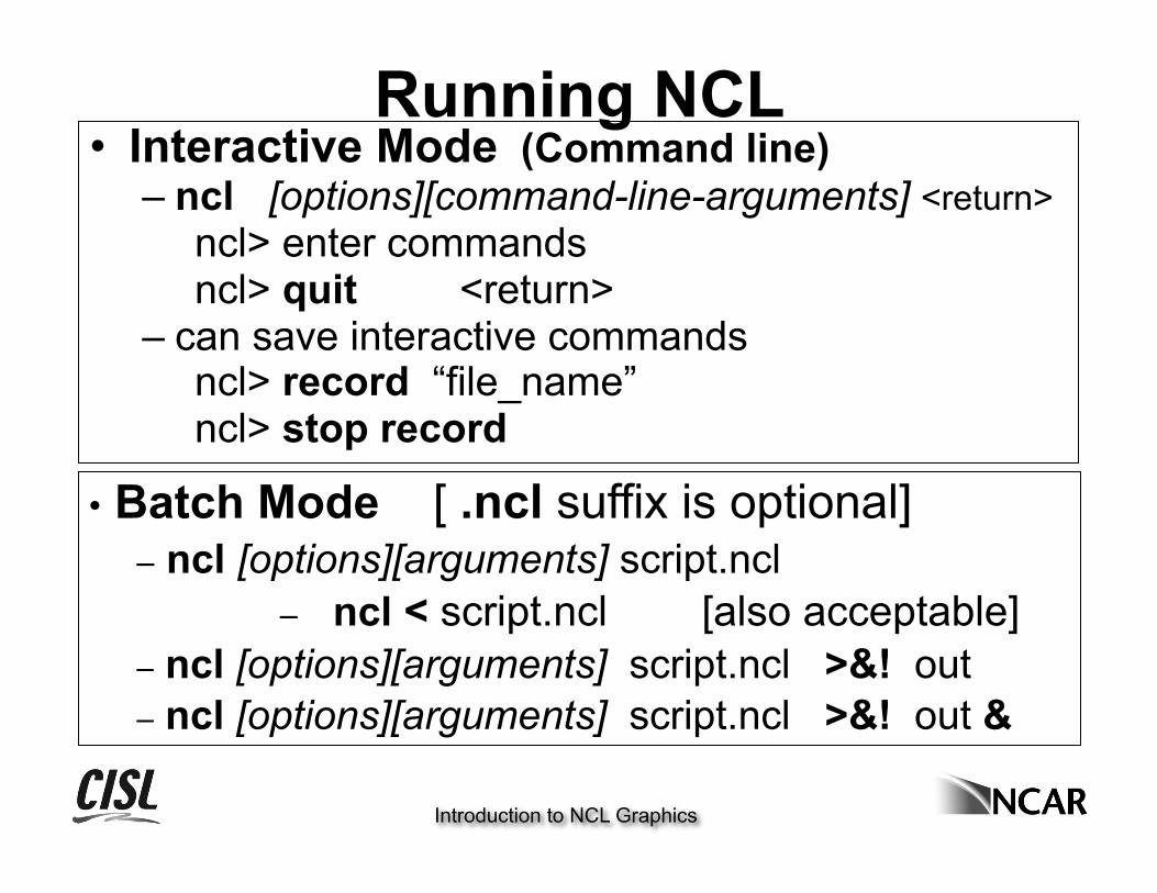
Running NCL • Interactive Mode (Command line)
– ncl [options][command-line-arguments] <return> ncl> enter commands ncl> quit <return>
– can save interactive commands ncl> record “file_name” ncl> stop record
• Batch Mode [ .ncl suffix is optional] – ncl [options][arguments] script.ncl
– ncl < script.ncl [also acceptable] – ncl [options][arguments] script.ncl >&! out – ncl [options][arguments] script.ncl >&! out &
Introduction to NCL Graphics
NCL Graphics - the basics
• The minimum steps needed to create a plot • How resources (plot options) work • NCL variable overview • Where to try some exercises or download
example scripts and data • Useful documentation links
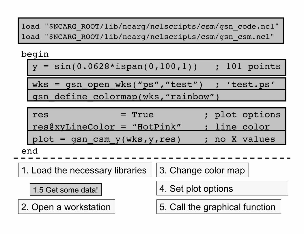
load "$NCARG_ROOT/lib/ncarg/nclscripts/csm/gsn_code.ncl" load "$NCARG_ROOT/lib/ncarg/nclscripts/csm/gsn_csm.ncl"
begin y = sin(0.0628*ispan(0,100,1)) ; 101 points
wks = gsn_open_wks(“ps”,”test”) ; ‘test.ps’ gsn_define_colormap(wks,“rainbow”)
res = True ; plot options res@xyLineColor = “HotPink” ; line color plot = gsn_csm_y(wks,y,res) ; no X values end
1. Load the necessary libraries
2. Open a workstation 5. Call the graphical function
4. Set plot options 1.5 Get some data!
3. Change color map
Introduction to NCL Graphics
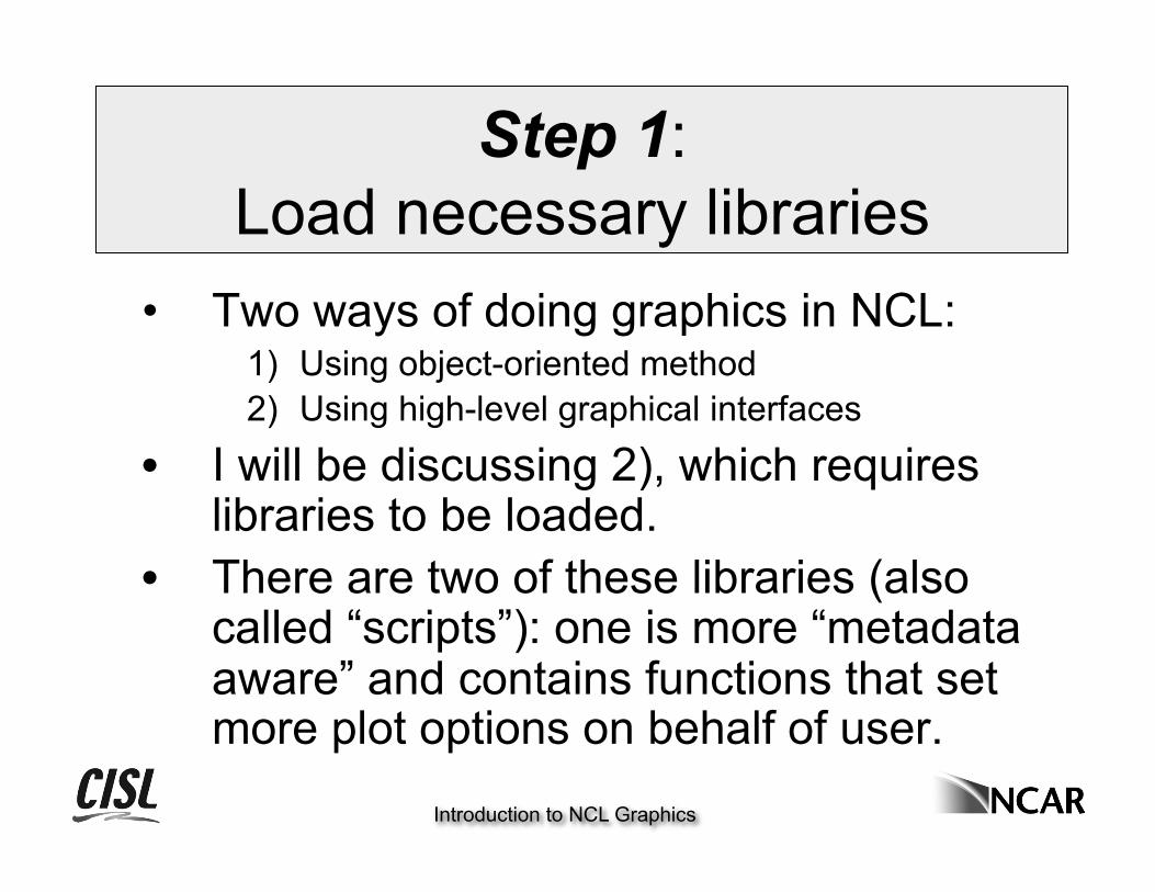
Step 1: Load necessary libraries
• Two ways of doing graphics in NCL: 1) Using object-oriented method 2) Using high-level graphical interfaces
• I will be discussing 2), which requires libraries to be loaded.
• There are two of these libraries (also called “scripts”): one is more “metadata aware” and contains functions that set more plot options on behalf of user.
Introduction to NCL Graphics
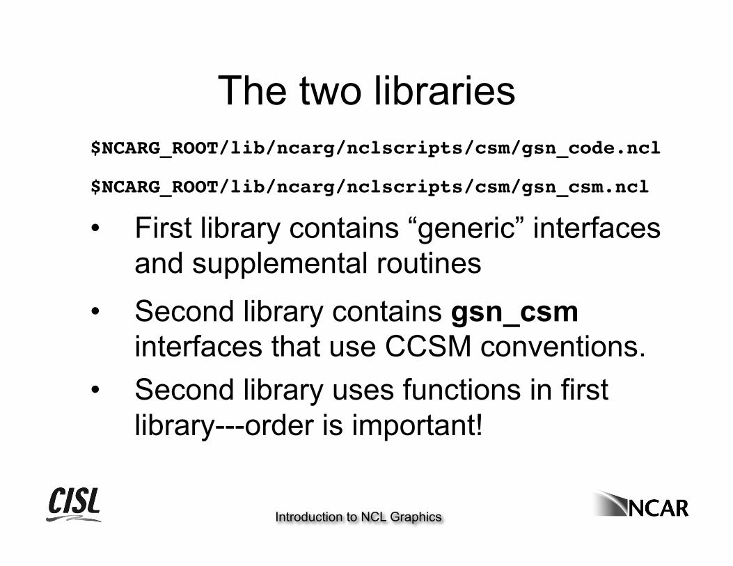
The two libraries
• Second library contains gsn_csm interfaces that use CCSM conventions.
• Second library uses functions in first library---order is important!
$NCARG_ROOT/lib/ncarg/nclscripts/csm/gsn_code.ncl
$NCARG_ROOT/lib/ncarg/nclscripts/csm/gsn_csm.ncl
• First library contains “generic” interfaces and supplemental routines
Introduction to NCL Graphics
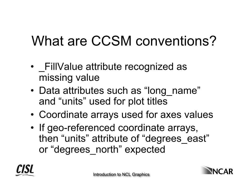
What are CCSM conventions?
• _FillValue attribute recognized as missing value
• Data attributes such as “long_name” and “units” used for plot titles
• Coordinate arrays used for axes values • If geo-referenced coordinate arrays,
then “units” attribute of “degrees_east” or “degrees_north” expected
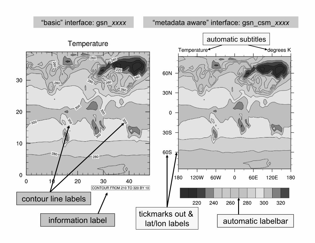
information label
contour line labels
“basic” interface: gsn_xxxx
automatic labelbar
automatic subtitles
tickmarks out & lat/lon labels
“metadata aware” interface: gsn_csm_xxxx
Introduction to NCL Graphics
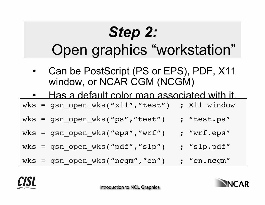
Step 2: Open graphics “workstation”
• Can be PostScript (PS or EPS), PDF, X11 window, or NCAR CGM (NCGM)
• Has a default color map associated with it, but you will probably want to change this (more later)
• Can have up to 15 multiple workstations open
• A “frame” means a “page”
wks = gsn_open_wks(“x11”,”test”) ; X11 window
wks = gsn_open_wks(“ps”,”test”) ; “test.ps”
wks = gsn_open_wks(“eps”,”wrf”) ; “wrf.eps”
wks = gsn_open_wks(“pdf”,”slp”) ; “slp.pdf”
wks = gsn_open_wks(“ncgm”,”cn”) ; “cn.ncgm”
Introduction to NCL Graphics
Step 3: Change the color map (opt’l)
• Do this before drawing to the frame.
• If you use the same color map a lot, can put in “.hluresfile” (more later)
• Can use one of the other 40+ color maps, or create your own.
• If you don’t change the color map, here’s what you’ll get…
gsn_define_colormap(wks,”rainbow”)
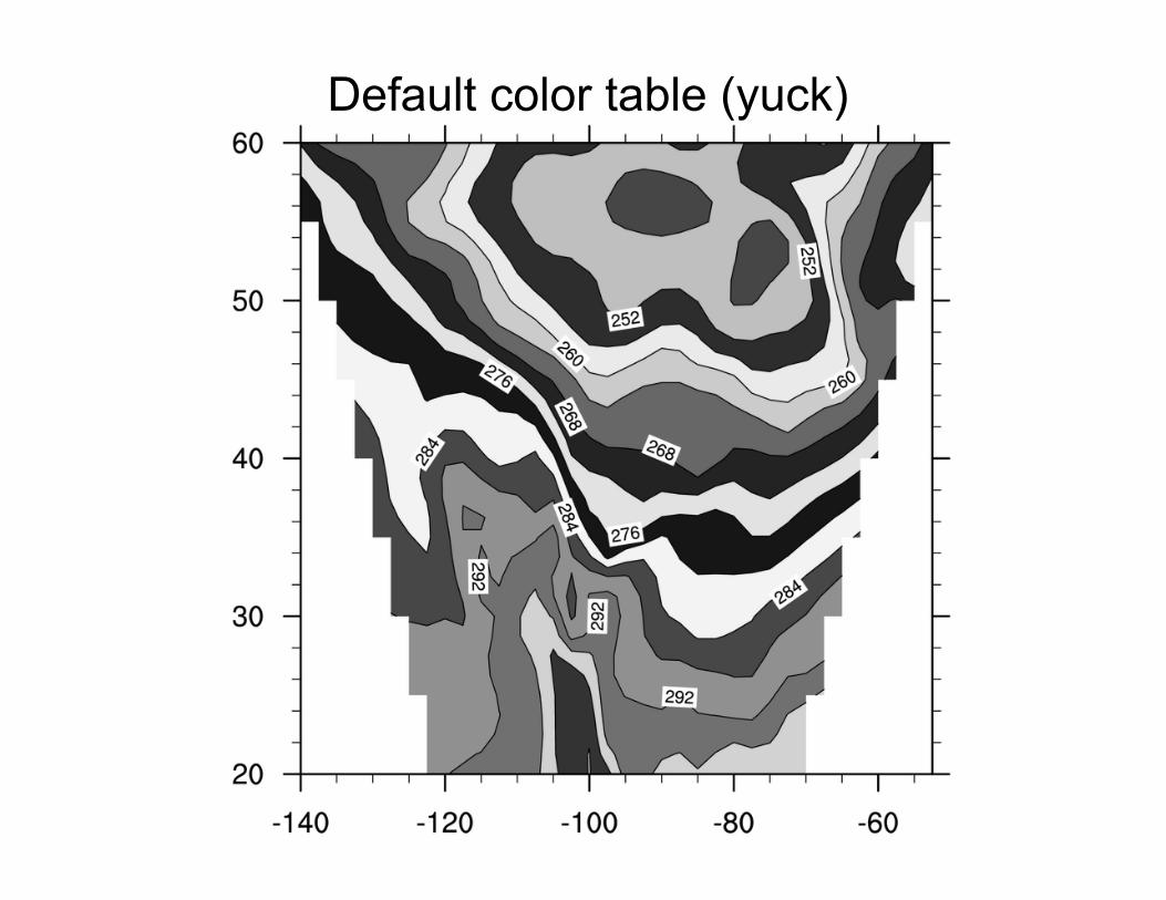
Default color table (yuck)
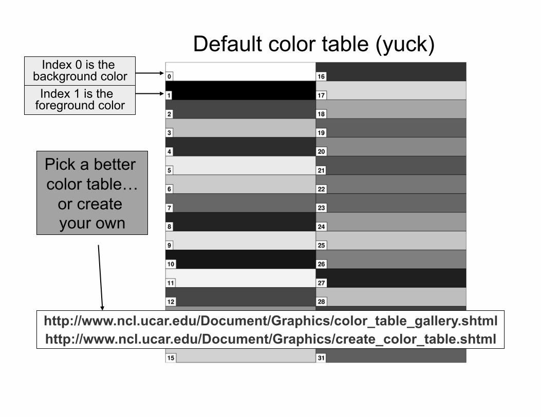
Default color table (yuck) Index 1 is the
foreground color
Index 0 is the background color
http://www.ncl.ucar.edu/Document/Graphics/color_table_gallery.shtml http://www.ncl.ucar.edu/Document/Graphics/create_color_table.shtml
Pick a better color table…
or create your own
Introduction to NCL Graphics
Step 4: Set optional resources
• Resources are the heart of your NCL graphics code.
• There are over 1,400 resources! • Resources are grouped by object type. • There are 11 “graphical” objects:
contours, labelbars, legends, maps, primitives, streamlines, text strings, tickmarks, titles, vectors, XY plots
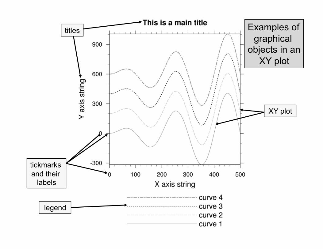
titles
legend
tickmarks and their
labels
XY plot
Examples of graphical
objects in an XY plot
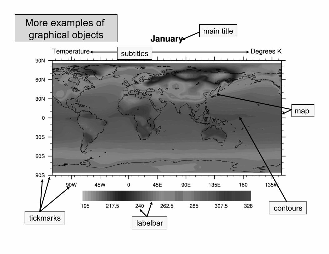
tickmarks contours
main title
subtitles
map
labelbar
More examples of graphical objects
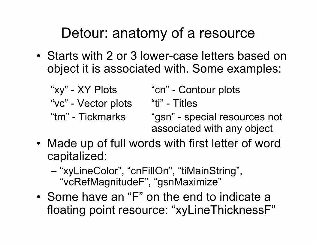
Detour: anatomy of a resource • Starts with 2 or 3 lower-case letters based on
object it is associated with. Some examples:
“xy” - XY Plots “cn” - Contour plots “vc” - Vector plots “ti” - Titles “tm” - Tickmarks “gsn” - special resources not
associated with any object • Made up of full words with first letter of word
capitalized: – “xyLineColor”, “cnFillOn”, “tiMainString”,
“vcRefMagnitudeF”, “gsnMaximize” • Some have an “F” on the end to indicate a
floating point resource: “xyLineThicknessF”
Introduction to NCL Graphics
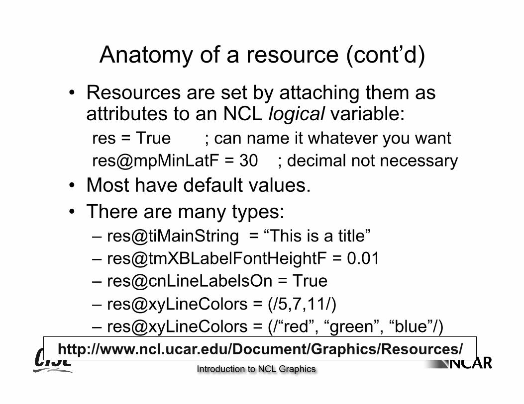
• Resources are set by attaching them as attributes to an NCL logical variable: res = True ; can name it whatever you want res@mpMinLatF = 30 ; decimal not necessary
• Most have default values. • There are many types:
– res@tiMainString = “This is a title” – res@tmXBLabelFontHeightF = 0.01 – res@cnLineLabelsOn = True – res@xyLineColors = (/5,7,11/) – res@xyLineColors = (/“red”, “green”, “blue”/) – res@lgLineThicknesses = (/ 1.0, 2.0, 3/) http://www.ncl.ucar.edu/Document/Graphics/Resources/
Anatomy of a resource (cont’d)
Introduction to NCL Graphics
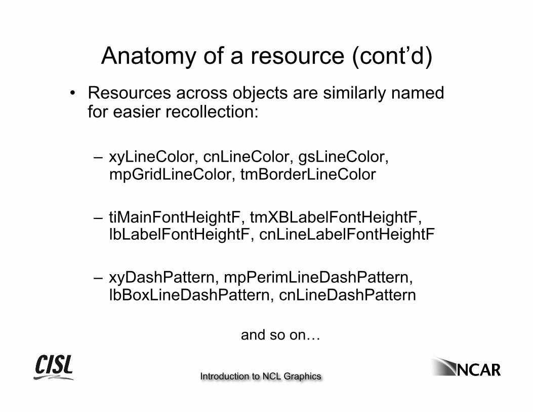
• Resources across objects are similarly named for easier recollection:
– xyLineColor, cnLineColor, gsLineColor, mpGridLineColor, tmBorderLineColor
– tiMainFontHeightF, tmXBLabelFontHeightF, lbLabelFontHeightF, cnLineLabelFontHeightF
– xyDashPattern, mpPerimLineDashPattern, lbBoxLineDashPattern, cnLineDashPattern
and so on…
Anatomy of a resource (cont’d)
Introduction to NCL Graphics
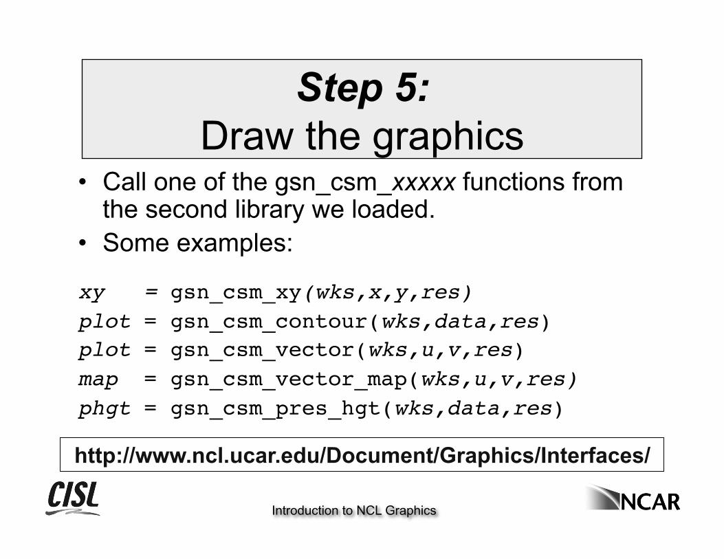
Step 5: Draw the graphics
• Call one of the gsn_csm_xxxxx functions from the second library we loaded.
• Some examples:
xy = gsn_csm_xy(wks,x,y,res) plot = gsn_csm_contour(wks,data,res) plot = gsn_csm_vector(wks,u,v,res) map = gsn_csm_vector_map(wks,u,v,res) phgt = gsn_csm_pres_hgt(wks,data,res)
http://www.ncl.ucar.edu/Document/Graphics/Interfaces/
Introduction to NCL Graphics
Now for some actual NCL graphics code samples…
Scripts have names like xy1a.ncl, xy1b.ncl, …
The first one is usually one with no resources set, and each subsequent script adds a few more resources.
NCL scripts that follow can be viewed and downloaded from the web:
http://www.ncl.ucar.edu/Training/Workshops/Scripts/
Scripts and sample datasets may also be
available on your machine.
Introduction to NCL Graphics
In review…
• Five steps to create a plot • Use X11 window while debugging script;
move to PS/PDF later • Hardest part are the resources: start
simple • Organize resources for easier debugging • Start with an existing script if possible
Introduction to NCL Graphics
NCL Variables Must begin with an alphabetic character May contain any mix of numeric and alphabetic
characters One exception: the underscore _ is allowed Variable names ARE case-sensitive Max name length is 256 characters Examples: a A forecast_time __t__
Introduction to NCL Graphics
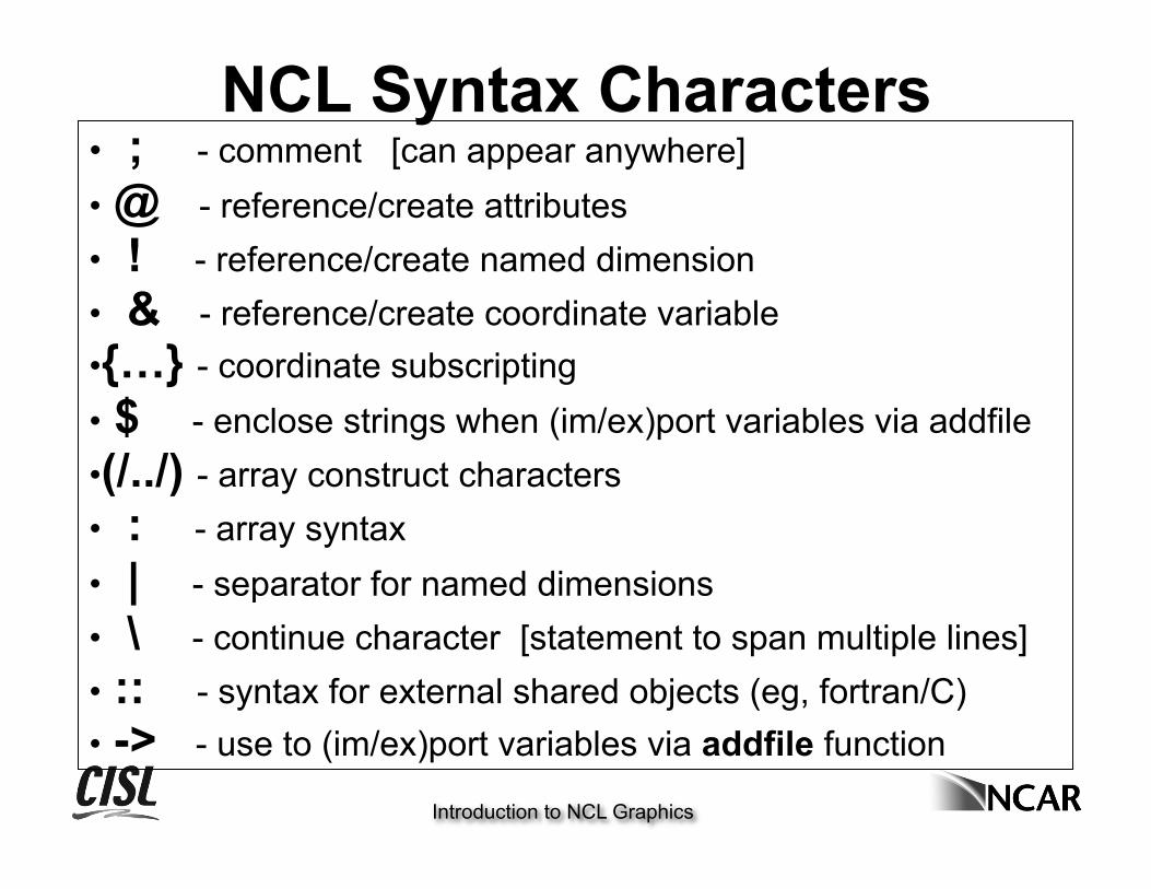
NCL Syntax Characters • ; - comment [can appear anywhere] • @ - reference/create attributes • ! - reference/create named dimension • & - reference/create coordinate variable • {…} - coordinate subscripting • $ - enclose strings when (im/ex)port variables via addfile • (/../) - array construct characters • : - array syntax • | - separator for named dimensions • \ - continue character [statement to span multiple lines] • :: - syntax for external shared objects (eg, fortran/C) • -> - use to (im/ex)port variables via addfile function
Introduction to NCL Graphics
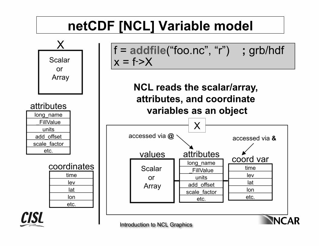
netCDF [NCL] Variable model
f = addfile(“foo.nc”, “r”) ; grb/hdf x = f->X
X Scalar
or Array
attributes long_name _FillValue
units add_offset
scale_factor etc. values
Scalar or
Array
attributes long_name _FillValue
units add_offset
scale_factor etc.
accessed via @ accessed via &
time lev lat lon etc.
coordinates time lev lat lon etc.
coord var
NCL reads the scalar/array, attributes, and coordinate
variables as an object X
Introduction to NCL Graphics
Customize your graphics environment Optional, but most highly recommended.
• Download “.hluresfile” file, put in home directory – Changes your default background, foreground colors
from black/white to white/black – Changes font from times-roman to helvetica – Changes “function code” (default is a colon) – Can be used to change default color map
• Available on your lab machines: cat ~/.hluresfile
http://www.ncl.ucar.edu/Document/Graphics/hlures.shtml
(Come to think of it, not really that optional!)
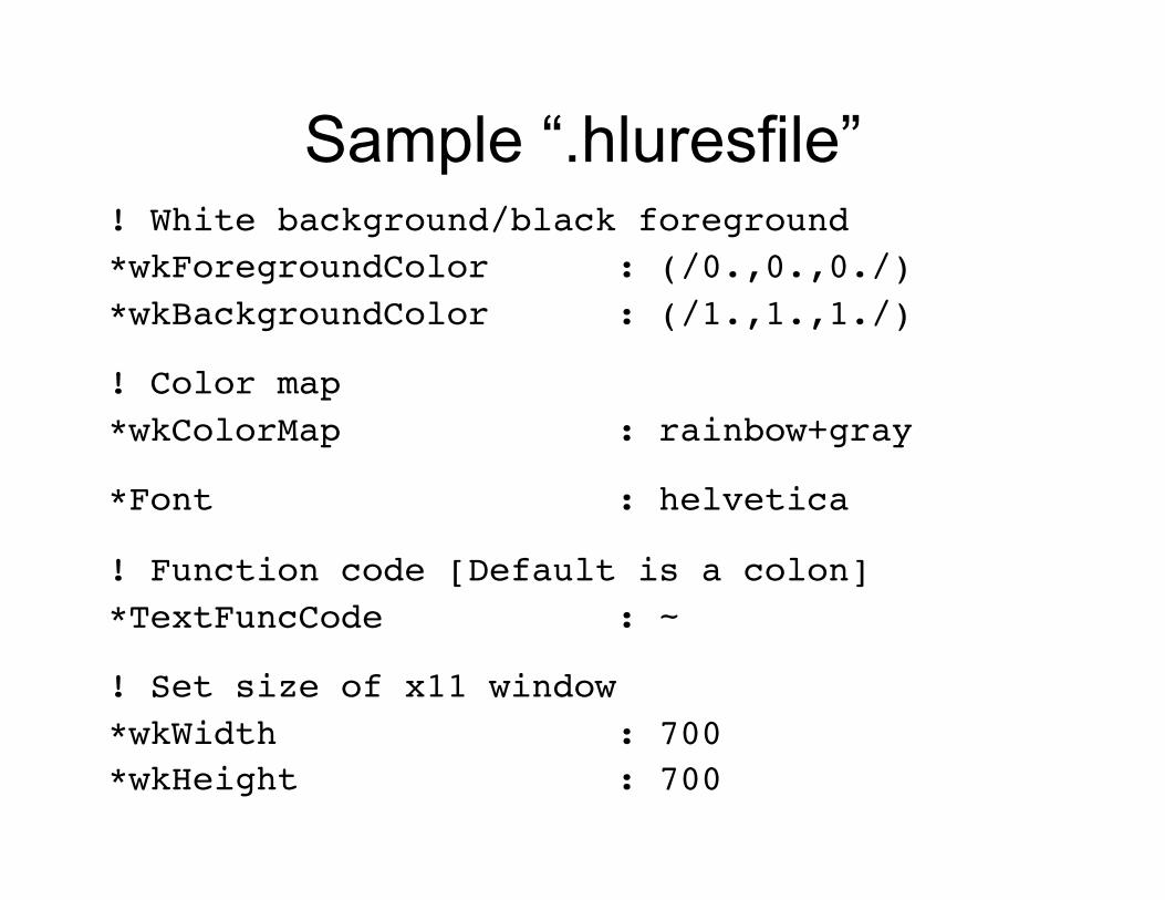
Sample “.hluresfile” ! White background/black foreground *wkForegroundColor : (/0.,0.,0./) *wkBackgroundColor : (/1.,1.,1./)
! Color map *wkColorMap : rainbow+gray
*Font : helvetica
! Function code [Default is a colon] *TextFuncCode : ~
! Set size of x11 window *wkWidth : 700 *wkHeight : 700

Common mistakes or problems http://www.ncl.ucar.edu/Document/Graphics/error_msg.shtml
• Forgot .hluresfile (fonts will look wrong) • “xyLineColour” is not a resource in XyPlot at
this time” – Misspelling a resource, “xyLineColour” – Using the wrong resource with the wrong plot (i.e.
using “vcRefMagnitudeF” in a contour plot).
• “The units attribute of the Y coordinate array is not set to one of the allowable units values (i.e. 'degrees_north'). Your latitude labels may not be correct.” – Lack of (or wrong) “units” attribute attached to your
data’s coordinate arrays

More common mistakes or problems • Data values in plot look off-scale
– Maybe “_FillValue” attribute not set or not correct.
• Not getting gray-filled lands in map plots. – You are using a color map that doesn’t have gray
in it (use “NhlNewColor” to add gray or change color maps to one that has gray).
• “_NhlCreateSplineCoordApprox: Attempt to create spline approximation for Y axis failed: consider adjusting trYTensionF value” – Data is too irregularly spaced in the X or Y
direction. May need to subset it.
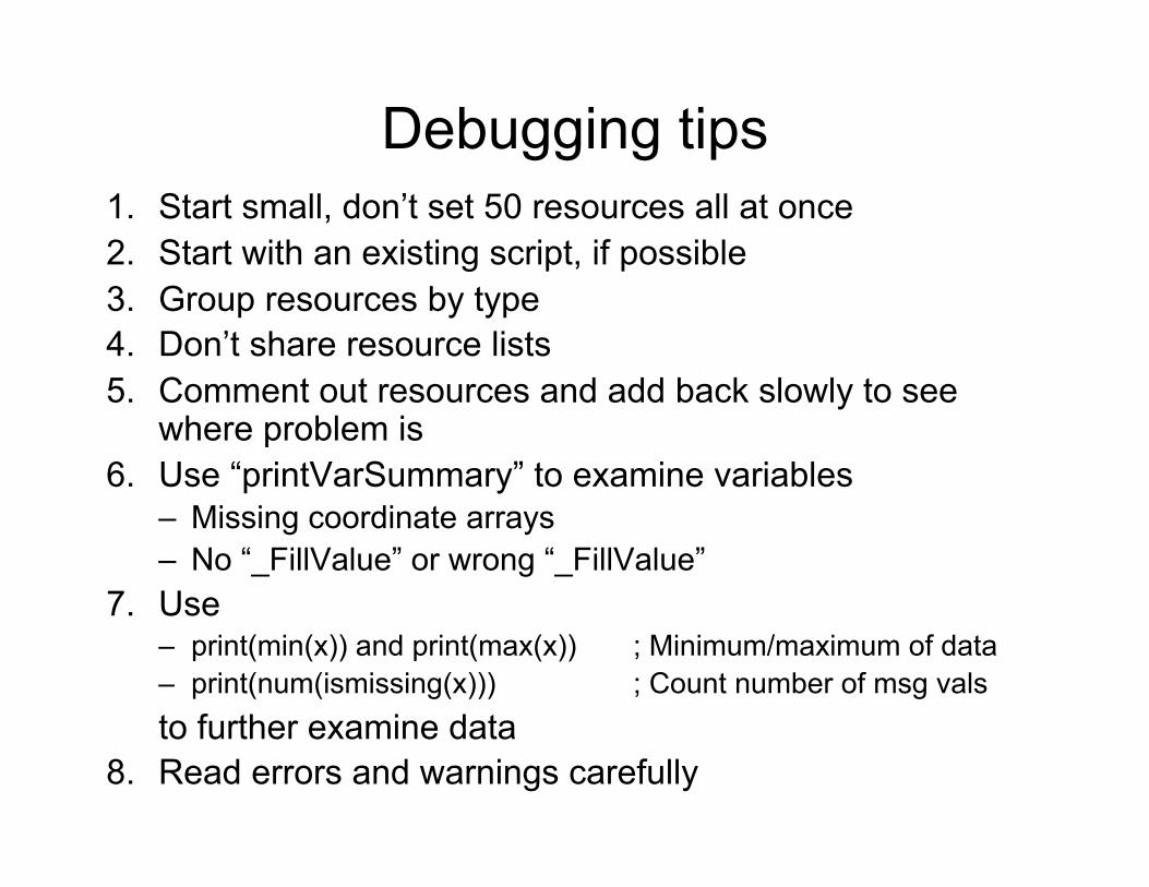
Debugging tips 1. Start small, don’t set 50 resources all at once 2. Start with an existing script, if possible 3. Group resources by type 4. Don’t share resource lists 5. Comment out resources and add back slowly to see
where problem is 6. Use “printVarSummary” to examine variables
– Missing coordinate arrays – No “_FillValue” or wrong “_FillValue”
7. Use – print(min(x)) and print(max(x)) ; Minimum/maximum of data – print(num(ismissing(x))) ; Count number of msg vals to further examine data
8. Read errors and warnings carefully
Introduction to NCL Graphics
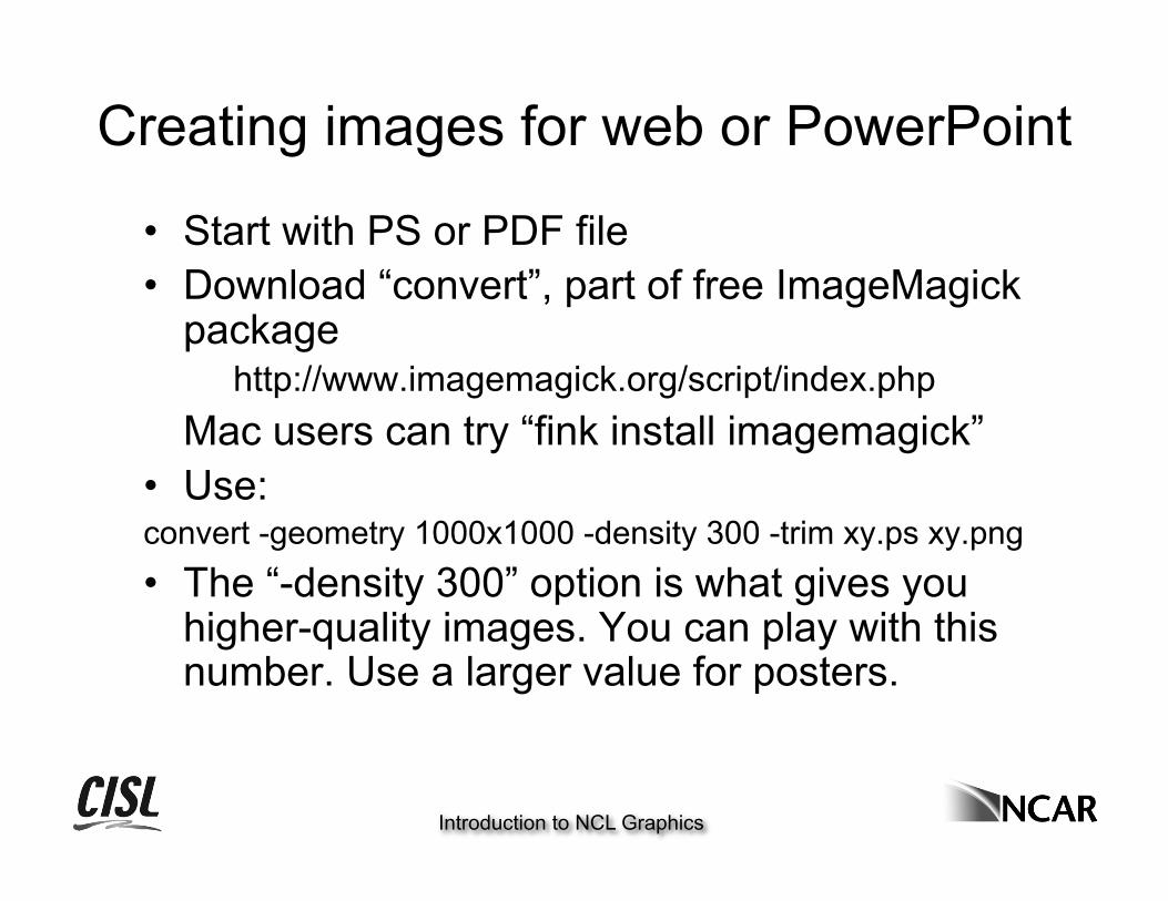
Creating images for web or PowerPoint • Start with PS or PDF file • Download “convert”, part of free ImageMagick
package http://www.imagemagick.org/script/index.php
Mac users can try “fink install imagemagick” • Use: convert -geometry 1000x1000 -density 300 -trim xy.ps xy.png • The “-density 300” option is what gives you
higher-quality images. You can play with this number. Use a larger value for posters.
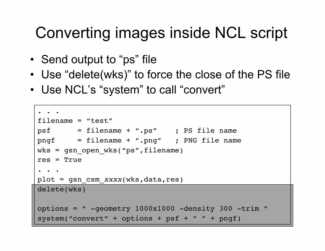
Converting images inside NCL script • Send output to “ps” file • Use “delete(wks)” to force the close of the PS file • Use NCL’s “system” to call “convert”
. . . filename = “test” psf = filename + “.ps” ; PS file name pngf = filename + “.png” ; PNG file name wks = gsn_open_wks(“ps”,filename) res = True . . . plot = gsn_csm_xxxx(wks,data,res) delete(wks)
options = “ -geometry 1000x1000 -density 300 -trim ” system(“convert“ + options + psf + “ “ + pngf)


![[Tut]How to Crack WPA_2-PSK W_ BT4 [Tut]](https://static.documents.pub/doc/80x56/577d28121a28ab4e1ea52a3b/tuthow-to-crack-wpa2-psk-w-bt4-tut.jpg)


